Research ArticleTwo-Layer Linear MPC Approach Aimed at Walking BeamBillets Reheating Furnace Optimization

Silvia Maria Zanoli and Crescenzo Pepe

Dipartimento di Ingegneria dellrsquoInformazione Universita Politecnica delle Marche Ancona Italy

Correspondence should be addressed to Silvia Maria Zanoli szanoliunivpmit

Received 23 September 2016 Revised 18 November 2016 Accepted 21 December 2016 Published 31 January 2017

Academic Editor Shuyou Yu

Copyright copy 2017 Silvia Maria Zanoli and Crescenzo Pepe This is an open access article distributed under the Creative CommonsAttribution License which permits unrestricted use distribution and reproduction in any medium provided the original work isproperly cited

In this paper the problem of the control and optimization of a walking beam billets reheating furnace located in an Italian steel plantis analyzed An ad hoc Advanced Process Control framework has been developed based on a two-layer linear Model PredictiveControl architecture This control block optimizes the steady and transient states of the considered process Two main problemshave been addressed First in order to manage all process conditions a tailored module defines the process variables set to beincluded in the control problem In particular a unified approach for the selection on the control inputs to be used for controlobjectives related to the process outputs is guaranteed The impact of the proposed method on the controller formulation is alsodetailed Second an innovative mathematical approach for stoichiometric ratios constraints handling has been proposed togetherwith their introduction in the controller optimization problems The designed control system has been installed on a real plantreplacing operatorsrsquo mental model in the conduction of local PID controllers After two years from the first startup a strong energyefficiency improvement has been observed

1 Introduction

In recent decades process industries observed importantchanges and increasing need for technological improvementsin the production units has been supported by an increasinglevel of automation In this context the migration towardmore profitable control and optimization solutions hasbeen registered aimed at the research of optimal trade-offsbetween throughput and yields increasing costs reductionand product quality improvement [1]

In particular a profitable balance between the meetingof precise production and quality specifications and theachievement of energy efficiency complying with rigorousenvironmental standards has to be ensured For this pur-pose minimum payback time solutions are preferred byprocess engineers and managers These smart solutions aimat a maximum exploitation of the already existent devicessoftware strategies are preferred to hardware modificationsintroducing Advanced Process Control (APC) systems [2 3]

Among APC solutions Model Predictive Control (MPC)architectures have shown their soundness and strong reliabil-ity in control and optimization of multivariable constrained

industrial processes [4 5] MPC implementation in processindustries ismainly due to its formulation flexibility differentcost functions subject to different types of constraints can besuitably designed [6 7]

In this paper a developed APC framework for the controland the optimization of a walking beam billets reheatingfurnace located in an Italian steel plant is described In thecontrol literature different control solutions for this controlproblem have been proposed In [8] a computer controlsystem for optimization of reheating furnaces has beendeveloped which contains functions for fuel optimizationbased on carpet diagrams and delay strategy multipliers Ahybrid optimization setpoint strategy for reheating furnacestemperatures is proposed in [9] based on steady statezone temperature optimization and dynamic optimizationperformed by PID controllers In [10] a dynamic model ofthe reheating furnace is derived using material and energybalances and a multivariable predictive controller designprocedure is proposed In [11] the potential of nonlinearMPC techniques to improve the temperature control of themetal slabs in a hot mill reheat furnace is explored in

HindawiJournal of Control Science and EngineeringVolume 2017 Article ID 5401616 15 pageshttpsdoiorg10115520175401616

2 Journal of Control Science and Engineering

particular a focus on energy consumption decreasing is pre-sented A Lyapunov-based MIMO state feedback controlleris developed for slab temperatures in a continuous fuel-firedreheating furnace in [12] The controller modifies referencetrajectories of furnace temperatures and is part of a cascadecontrol scheme In [13] a nonlinear MPC is designed for acontinuous reheating furnace for steel slabs Based on a first-principles mathematical model the controller defines localfurnace temperatures so that the slabs reach their desiredfinal temperatures In [14] an MPC based control method isdeveloped for the accurate control of cooling temperature in ahot-rolled strip laminar cooling process exploiting a tailoredextended Kalman filter to observe the spatial distribution ofstrip temperature in water cooling section

The proposed approach is based on a two-layer linearMPC architecture and addressed tailored control specifica-tions In particular the linear approach allowed limiting thecomputational burden while the introduction of two maincontrol modes ensured an effective control system [15]

In this paper two control requirements have been specif-ically addressed First a unified approach for the selection ofthe control inputs to exploit for control objectives fulfilmenthas been formulated for all process conditions For thispurpose a suitablemodule has been introducedwhich tightlycooperates with a two-layer linearMPC block Furthermorea decoupling strategy developed by the authors in a previouswork [16] has been suitably extended so to include a properhandling of all process conditions Second an innovativemathematical approach aimed at stoichiometric ratios con-straints tightening has been proposed

Accurate simulations have proven the validity of theproposed approaches The successive implementation of thedesigned controller on the industrial process successfullyreplaced the operatorsrsquo manual driving of local PID con-trollers

The paper is organized as follows the analyzed walkingbeam billets reheating furnace is accurately described inSection 2 together with the control specifications and thedeveloped process modelling Section 3 details the developedAPC framework explaining the functions of the variousblocks and how the proposed solutions impact the for-mulations of the two MPC layers Tuning procedures andsimulation examples have been depicted in Section 4 whileSection 5 describes observed field results Finally conclusionshave been reported in Section 6

2 The Studied Billets Reheating Furnace

This section discusses the analyzed industrial process thatis a walking beam billets reheating furnace This processrepresents the most significant phase of an Italian steel plantProcess features together with the control requirements andthe process modelling are detailed

21 Process Characterization The production chain of thestudied Italian steel industry is schematically depicted inFigure 1

Raw materials for example waste steel products areprocessed in the first phase so as to obtain small steel bars

at an intermediate stage of manufactureThese bars are calledbillets In the investigated process billets are characterized bya rectangular (020 [m] times 016 [m]) or a quadratic (016 [m] times016 [m] or 015 [m] times 015 [m]) section and their length canbe 45 [m] or 9 [m]

The billets are then introduced in a reheating furnaceThe considered reheating furnace measures 24 [m] and it cancontain up to 80 billets simultaneously When they enter thefurnace the billets can be characterized by very differenttemperatures These input temperatures vary from 30[∘C] to700[∘C] The billets that are inside the furnace are reheatedbased on specific temperature profiles In this way at thefurnace exit billets temperature can vary according to thespecifications of the subsequent rolling phase Typical billetexit temperatures vary in the range of 1000[∘C]ndash1100[∘C]After their path along the furnace the billets are movedtoward the rolling mill stands here they are subjected to aplastic deformation suitably performed by stands cylindersThese cylinders deform the reheated billets according tothe finished products specifications Examples of finishedproducts are angle bars iron rods or tube rounds

The present paper is focused on the reheating phasethat is the crucial phase in a steel industry The importanceof this phase is due to the high energy amount requiredin order to achieve energy efficiency an optimal trade-off between conflicting requirements that is environmentalimpact decreasing energy saving and product and productquality increasing has to be ensured

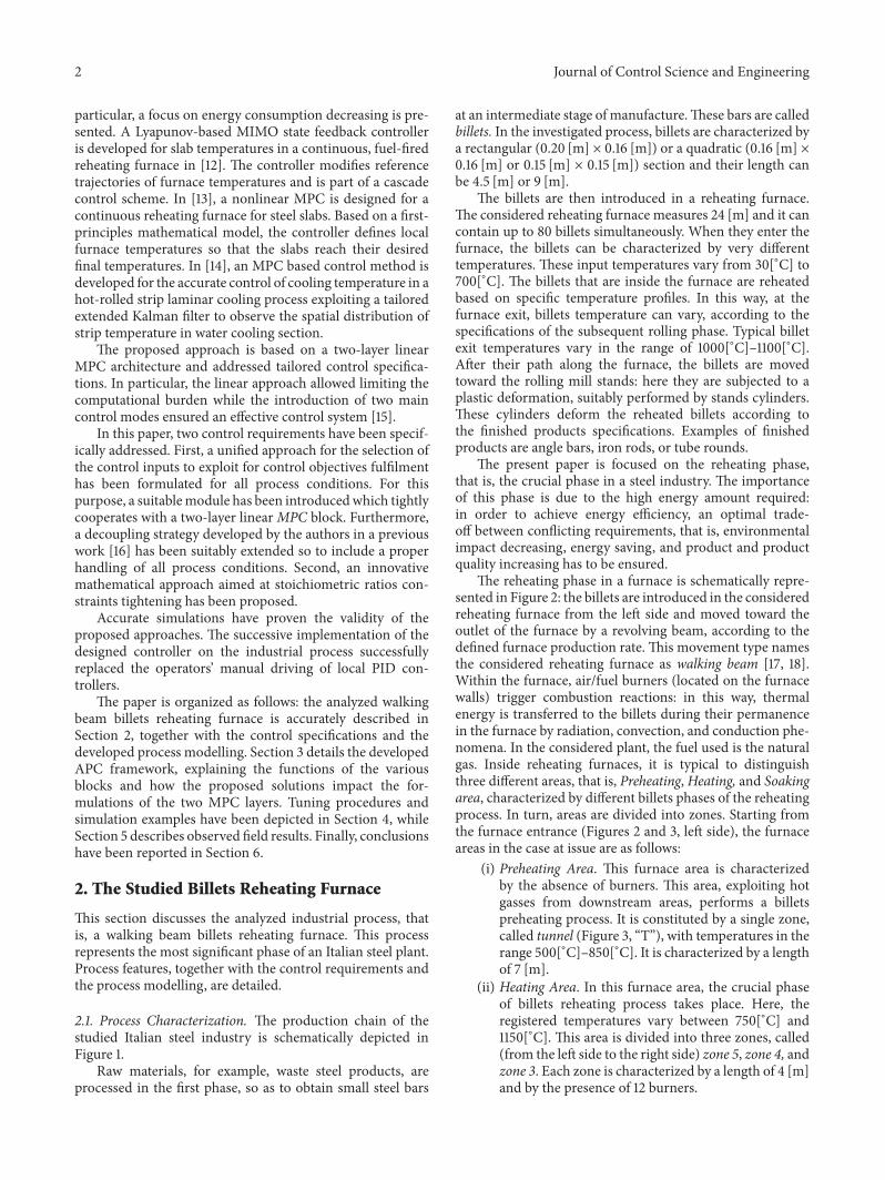
The reheating phase in a furnace is schematically repre-sented in Figure 2 the billets are introduced in the consideredreheating furnace from the left side and moved toward theoutlet of the furnace by a revolving beam according to thedefined furnace production rate This movement type namesthe considered reheating furnace as walking beam [17 18]Within the furnace airfuel burners (located on the furnacewalls) trigger combustion reactions in this way thermalenergy is transferred to the billets during their permanencein the furnace by radiation convection and conduction phe-nomena In the considered plant the fuel used is the naturalgas Inside reheating furnaces it is typical to distinguishthree different areas that is PreheatingHeating and Soakingarea characterized by different billets phases of the reheatingprocess In turn areas are divided into zones Starting fromthe furnace entrance (Figures 2 and 3 left side) the furnaceareas in the case at issue are as follows

(i) Preheating Area This furnace area is characterizedby the absence of burners This area exploiting hotgasses from downstream areas performs a billetspreheating process It is constituted by a single zonecalled tunnel (Figure 3 ldquoTrdquo) with temperatures in therange 500[∘C]ndash850[∘C] It is characterized by a lengthof 7 [m]

(ii) Heating Area In this furnace area the crucial phaseof billets reheating process takes place Here theregistered temperatures vary between 750[∘C] and1150[∘C] This area is divided into three zones called(from the left side to the right side) zone 5 zone 4 andzone 3 Each zone is characterized by a length of 4 [m]and by the presence of 12 burners

Journal of Control Science and Engineering 3

Raw materials processing phase

Reheating phase

Rolling phase

Billets Reheatedbillets

Raw materials Finishedproducts

Figure 1 Workflow of the considered Italian steel industry

Tunnel Zones 5-4-3 Zones 2-1

Preheatingarea

Heatingarea

Soakingarea

Figure 2 Representation of the considered walking beam billets reheating furnace

T 5 4 32

1

Figure 3 Schematic furnace zones disposition

(iii) Soaking Area In this last furnace area the billets com-plete their reheating process Here temperatures varyapproximately in the range 1100[∘C]ndash1250[∘C] and thetotal length is 5 [m] The furnace area equipped with24 burners is transversally divided into two zonesdenoted as zone 2 and zone 1 (Figure 3)

Billets during their traverse through the furnace aresubjected to monotonically increasing temperatures At thebeginning of the Preheating area is located a heat exchangerdenoted as smoke-exchanger This allows the heat recoverfrom the combustion smokes of the various furnace areaswhich is used for the preheating of the combustion airprovided to each burner

22 Process Instrumentation and Control Requirements Inthe considered reheating furnace measurements of the tem-perature of each furnace zone and of the smoke-exchangerare acquired by thermocouples suitably positioned within thefurnaceTheHeating and Soaking furnace areas are equippedwith flowmeters for fuel (natural gas) and air flow ratesmeasurement Air and furnace pressure are measured by

manometers The billets temperature at their entrance in thefurnace are registered by an optical pyrometer An additionalpyrometer measures the temperature of the processed billetsBillets transition at the furnace inlet and outlet is detected byphotocells

Before the introduction of the proposed APC system thereheating furnace was regulated by plant operatorsrsquo manualconduction of local PID controllers Operators based on thefurnace conditions and on the production requirements setthe zones temperature targets manually

A great amount of thermal energy is required in a steelbillets reheating furnace With the previous control systemthe natural gas consumption per year was about 9 million[Sm3] related to a total steel production of approximately35000 [ton] The minimization of the fuel consumptiontogether with the furnace production rate maximizationclearly represents the crucial factor for energy efficiencyachieving and improvement In addition to these require-ments there is also the need to meet stringent qualitystandards of the finished products

After an initial study and analysis phase repeated and tar-getedmeetingswith plantmanagers engineers and operatorswere conducted and the followingmain control specificationshave been outlined for the considered APC design [19 20]

(I) Compliance with the required billets temperatureconstraints at their exit from the furnace based on thespecifications for the subsequent plastic deformationin the rolling mill phase

(II) Meeting of stoichiometry constraints related to airfuel ratios

(III) Meeting of total air flow rate and smoke-exchangertemperature limits so as to preserve furnace safety

4 Journal of Control Science and Engineering

Table 1 The Manipulated Variables

Variable name Acronym [units]Zone 119894 fuel flow rate (119894 = 1 5) Fuel119894 [Nm

3h]Zone 119894 air flow rate (119894 = 1 5) Air119894 [Nm

3h]

Table 2 The Disturbance Variables

Variable name Acronym [units]Furnace production rate Prod [th]Furnace pressure FurnPress [mmH2O]Air pressure AirPress [mbar]

Table 3 The main Controlled Variables

Variable name Acronym [units]Tunnel temperature Tun [∘C]Zone 119894 (119894 = 1 5) temperature Temp119894 [

∘C]Zone 1ndashzone 2 temp difference Diff 12 [∘C]Total air flow rate AirTot [Nm3h]Smoke-exchanger temperature SE [∘C]

(IV) Furnace management in all predictable conditions(V) Minimization of the fuel (natural gas) consumption

optimizing all furnace conditions (eg with a varyingfurnace production rate)

The simultaneousmeeting of all the above requirements isnot easily attainable by a manual conduction of the furnaceIn the conduction of the reheating furnace operators typi-cally neglected the aspects more strictly tied to energy savingand environmental impact decreasing being concentrated onassuring a suitable billets heating profile So with the previousfurnace management billets were often reheated more thanneeded by the subsequent rolling mill phase

23 Modelling the Considered Process In order to design anAPC system for furnace energy efficiency improvement anaccurate process modelling has been performed As widelyused in APC applications three main groups of processvariables have been identified Controlled Variables (CVs)Manipulated Variables (MVs) and Disturbance Variables(DVs) CVs are the process outputs (assumed all measured)their control is performed exploiting MVs and taking intoaccount DVs information in a feedforward way In factMVs and DVs represent the measured process inputs theAPC system can only act on MVs while DVs cannot bemodified by the APC system CVs have been included in a119910[119898119910times1] vector MVs and DVs have been grouped in a 119906[119897119906times1]vector and in a 119889[119897119889times1] vector respectively Tables 1 and 2depict MVs and DVs while key CVs have been reported inTable 3 In the CVs group the following process variableshave been included the temperature of each furnace zone(including tunnel) the difference between zone 1 and zone2 temperatures the smoke-exchanger temperature the totalair flow rate and the fuel and air valves opening (per cent)In the DVs group furnace production rate air pressure andfurnace pressure have been included Finally in the MVs

group air and fuel flow rates of each furnace zone have beenconsidered In the plant configuration fuel and air flow ratesare regulated through PID controllers the designed APCsystemwill provide the PID low level controllers with suitableset-points Their computation will be described in Section 3

An identification procedure based on a black-boxapproach has been conducted in order to obtain accuratedynamical models that could describe the selected pro-cess inputs (MVsDVs) and outputs (CVs) behaviour [21ndash23] First-order strictly proper asymptotically stable lineartime invariant models without delays have been obtainedIn these models deviations of the process variables fromconsistent operating points have been included Tables 4and 5 symbolically represent the CVs-MVs and CVs-DVsgain matrices 119866119910119906 [119898119910times119897119906] and 119866119910119889 [119898119910times119897119889] the gain sign of thetransfer functions that relate the MVs-DVs with the mainCVs is here reported Exploiting the identified models billetstemperature can be controlled with a suitable constrainedcontrol of the furnace zones temperature and of the temper-ature difference between the last two furnace zones (speci-fication (I) in Section 22) Furthermore smoke-exchangertemperature and total air flow rate can be controlled throughfuel and air flow rates (specification (III) in Section 22)Withregard to fuel and air flow rates usage plant engineers haveagreed on three additional requirements

(i) The temperature of all the furnace zones excepttunnel must be controlled exploiting only the relatedfuel flow rate

(ii) The temperatures of the tunnel and of the smoke-exchanger must be controlled exploiting only zone 5and zone 4 fuel flow rates

(iii) The total air flow rate must be regulated using onlyzone 5 and zone 4 air flow rates

In order to fulfil these additional objectives an extendeddecoupling strategy has been developed by the authors(Sections 32 and 33)

Each of the furnace zones equipped with burners mustcomply with stoichiometric constraints in order to guaranteeproper thermodynamic reactions In the considered casestudy five stoichiometric ratios have to be controlled Thesevariables have been grouped in 119911[119898119911times1] vector of ratio Con-trolled Variables (rCVs) Typical lower and upper constraintsfor the considered stoichiometric ratios have been summa-rized in Table 6 The stoichiometric ratios lower constraintsrepresent safety conditions their excessive violation can leadto a furnace stop The upper constraints avoid air excess inthe burnersrsquo combustion contributing to the achievement offurnace energy efficiency Stoichiometric ratios constraintshave been suitably handled by an innovative formulation inthe119872119875119862 block (Section 35)

The proposed extended decoupling strategy togetherwith additional procedures allows the optimization of all fur-nace conditions searching for fuel minimization directions

Journal of Control Science and Engineering 5

Table 4 The CVs-MVs mapping matrix

Acronym Fuel5 Fuel4 Fuel3 Fuel2 Fuel1 Air5 Air4 Air3 Air2 Air1Tun + + + + +Temp5 + + + + + minusTemp4 + + + + minusTemp3 + + + minusTemp2 + + minusTemp1 + + minusDiff 12 minus +AirTot + + + + +SE + + + + +

Table 5 The CVs-DVs mapping matrix

Acronym Prod FurnPress AirPressTun minus + minusTemp5 minus + minusTemp4 minus + minusTemp3 minus + minusTemp2 minus + minusTemp1 minus + minusDiff 12AirTotSE minus + minus

Table 6 The ratio Controlled Variables constraints

Variable name Acronym[units]

Lowerconstraint

Upperconstraint

Zone 5 stoichiometricratio 1198775 [] 108 123

Zone 4 stoichiometricratio 1198774 [] 105 12

Zone 3 stoichiometricratio 1198773 [] 105 12

Zone 2 stoichiometricratio 1198772 [] 98 113

Zone 1 stoichiometricratio 1198771 [] 98 113

3 APC Framework

This section describes the APC framework designed forthe control and the optimization of the considered walkingbeam reheating furnaceThe various blocks are differentiatedtogether with their functions In particular the proposedcontrol solutions are detailed

31 Detailing the Scheme The APC architecture has beendepicted in Figure 4 Three main blocks can be noted Plantamp SCADA (PampS) block Data Conditioning amp DecouplingSelector (DCampDS) andMPC block

At each control instant 119896 PampS block based on a Supervi-soryControl andDataAcquisition (SCADA) system supplies

updated MVs DVs and CVs measurements (119906(119896 minus 1) 119889(119896 minus1) 119910(119896)) Additionally a status value (u-d-y-z status) for eachprocess variable is forwarded

DCampDS block detects abnormal situations exploitingfield data conditioning information and defines the finalstatus value for each variable (u-d-y status 119911 status) suit-ably processing PampS status information Depending on thevariable final status the variables set to be included inthe controller formulation at the current control instant isaccordingly modified Details about status handling havebeen explained by the authors in [24] In this work anextension of a decoupling strategy proposed by the authorsin a previous work ([16]) is formulated assuring a straightrelationship between the decoupling strategy and the MVsand CVs status values definition (DecouplingMatrix) In thisway a unified approach for the selection of MVs to exploitfor the fulfilment of CVs specifications has been guaranteedin all process conditions (Section 32)

The acquired information is forwarded to the linearModel Predictive Control (MPC) block characterized by atwo-layer architectureThis block is constituted by theTargetsOptimizing and Constraints Softening (TOCS)module at theupper level and the Dynamic Optimizer (DO) module at thelower lever both supported by the Predictions Calculatormodule These modules suitably cooperate computing theMVs value 119906(119896) to be applied to the plant at the currentcontrol instant

In both optimization problems MVs constraints areassumed as hard constraints they can never be violated andtheir feasibility has been suitably imposed As widely usedin MPC applications CVs constraints are assumed as softconstraints their softening is admitted in critical situationsthrough the introduction of suitable nonnegative slack vari-ables vectors denoted by 120576 An ad hoc approach has been ded-icated to rCVs constraints as it will be shown in Section 35

32 Data Conditioning amp Decoupling Selector Module TasksAn APC systemmust properly handle process variables in allprocess conditionsThe control system design has to take intoaccount all detectable situations Certain MVs DVs CVsor rCVs must be excluded from the controller formulationbased on abnormal situations (eg bad conditions or localcontrol loop faults) detection or on specific plant needs

6 Journal of Control Science and Engineering

MPC

target

Plant amp SCADA

Predictionscalculator

DO

TOCS

Data conditioning

amp decoupling selector

Decoupling Matrix

TOCS tuning parameters

constraints

constraints

DO tuning parameters

yConstraints

Decoupling Matrix

u-y

u-z

u-y-z

u(k minus 1) z statusu(k minus 1) d(k minus 1) y(k)

u(k minus 1) d(k minus 1) y(k)

u-d-y status

u-d-y-z status

u(k)

y free predictions

Figure 4 Architecture of the designed APC framework

In the designed APC scheme DCampDS block includeslogics aimed at a proper modification of the initial statusvalues supplied by PampS block (Figure 4 u-d-y-z status) asa consequence for example of spikes or freezing percentageviolation [24] These logics determine the final status valuesof all process variables (Figure 4 119911 status and u-d-y status)

In this work two status values have been consideredactive and inactive An active MV is used by MPC block forcontrol purposes while an inactive MV cannot be moved byMPC block for future predictions of the system behaviourits value is frozen to its last plant measurement (Figure 4119906(119896 minus 1)) When a CV (or a rCV) is active MPC block actsfor the satisfaction of the related control specifications whilewhen a CV (or a rCV) is inactive its control requirementsmust be ignored byMPC block

As stated in Section 2 MVsDVs-CVs relationships havebeen modelled with a linear time invariant asymptoticallystable model without delays

In order to include status value information on theprocess model a 119861119910119906 [119898119910times119897119906] matrix has been introduced anonzero entry on the generic (119894 119895) element represents anonzero relationship between the 119895th MV and the 119894th CVConsidering the gain matrix 119866119910119906 and defining with op =(sdot sdot)the element-wise inequality logical operation between twomatrices the binary matrix 119861119910119906 is obtained

119861119910119906 = op = (119866119910119906 0[119898119910times119897119906]) (1)

where 0[119898119910times119897119906] is a matrix with elements all equal to 0For the generic 119894th CV if this CV is active at the current

control instant all active MVs tied to it (ie the active MVscharacterized by a 1 on the related position on the 119894th rowof 119861119910119906 matrix) can act for its specifications fulfilment Inorder to admit additional degrees of freedom for the controlspecifications in a previous work the authors proposed asuitable decoupling strategy not dependent on the tuning

parameters This strategy enables for each CV the selectionof the MVs to exploit for its control purposes that isequivalently the inhibition of given MVs

Two equivalent mathematical approaches have been for-mulated [16] In this work the formulation based on thedefinition of a Decoupling Matrix is considered and suitablyextended

An initialDecouplingMatrix119863119864[119898119910times119897119906] is supplied byPampSblock (Figure 4) The generic (119894 119895) element of 119863119864 is set equalto 0 if both the following conditions hold

(i) The (119894 119895) element of 119861119910119906 matrix is equal to 1(ii) The 119895th MV must not be used to control the 119894th CV

Otherwise the (119894 119895) element is equal to 1The generic (119894 119895) nonzero element of the initial119863119864matrix

is zeroed byDCampDS block if at least one of the two followingconditions holds

(i) The 119894th CV is inactive(ii) The 119895th MV is inactive

The final 119863119864 matrix is then forwarded to TOCS and DOmodules

In the considered case study rCVs are represented by theratio between the related air and fuel flow ratesDCampDS blockprocesses the rCVs status value supplied by PampS block takinginto account the final status values of air and fuel flow rates(Figure 4 u-d-y status) In this way the final status valueassociated with each rCV is obtained (Figure 4 119911 status)Generally the 119894th stoichiometric ratio (119894 = 1 5) is definedas inactive if the 119894th fuel flow rate is inactive This means thatif the 119894th fuel flow rate is inactive the constraints of the 119894thstoichiometric ratio must be ignored byMPC block

33 Predictions Calculator and TOCS Modules Tasks Asstated before MPC block is composed of three modules

Journal of Control Science and Engineering 7

The two-layer linear MPC scheme exploits process variablespredictions on a prediction horizon119867119901 these predictions areparametrized on a defined number of MVs moves (assumedhere to be applied at the first 119867119906 prediction steps) calledcontrol horizon and denoted with119867119906 (0 lt 119867119906 le 119867119901) [25] Ateach control instant a sequence of MVs values is computedbut only the first value (Figure 4 119906(119896)) is forwarded tothe plant repeating the entire control algorithm at the nextcontrol instant (receding horizon strategy) [26 27]

Predictions Calculatormodule computes CVs free predic-tions over119867119901 (Figure 4 119910 free predictions) keepingMVs andDVs constant at their last field value (Figure 4 119906(119896 minus 1) and119889(119896 minus 1) resp) and taking into account the last CVs value(Figure 4 119910(119896)) for plant-model mismatch inclusion Futureinformation about DVs is assumed unknown so future DVstrends are assumed constant at 119889(119896 minus 1) value In CVs freepredictions computation CVs status values information isalso included

For the generic Vth CV predictions over119867119901 are expressedby

119910V (119896 + 119894 | 119896) = 119910freeV (119896 + 119894 | 119896) + Δ119910V (119896 + 119894 | 119896) (2)

Δ119910V (119896 + 119894 | 119896) = 119865119894V sdot Δ119880 (119896) (3)

Δ119880 (119896) =[[[[[[[

Δ (119896 | 119896)Δ (119896 + 1 | 119896)

Δ (119896 + 119867119906 minus 1 | 119896)

]]]]]]] (4)

where 119910freeV(119896+119894 | 119896) is the free prediction at the 119894th predictioninstant while Δ119910V(119896 + 119894 | 119896) is the related forced componentΔ119880(119896)[119897119906 sdot119867119906times1] is a vector that contains the 119867119906 MVs movesΔ(119896 + 119895 | 119896) (119895 = 0 119867119906 minus 1) assumed in the first 119867119906steps Δ(119896 + 119895 | 119896) terms are among the decision variablesof DO optimization problem (Section 34) The effects ofMVs moves on the 119894th prediction are modelled by 119865119894V [1times119897119906 sdot119867119906]vector

In this work the prediction horizon119867119901 is assumed to betuned so as to guarantee steady state reaching to the processmodel Based on this assumption the following relationshipholds

119866119910119906 = [[[[[

1198651198671199011 (1 (119895 minus 1) sdot 119897119906 + 1 119895 sdot 119897119906)119865119867119901119898119910 (1 (119895 minus 1) sdot 119897119906 + 1 119895 sdot 119897119906)

]]]]](119895 = 1 119867119906)

(5)

where 119865119867119901V(1 (119895 minus 1) sdot 119897119906 + 1 119895 sdot 119897119906) (V = 1 119898119910) is asubvector of 119865119867119901V of 119897119906 columns from the ((119895 minus 1) sdot 119897119906 + 1)thto the (119895 sdot 119897119906)th

The two-layer linear MPC scheme performs two opti-mization problems the first is solved by the upper layerrepresented by TOCS module while the second is relatedto the lower layer that is DO module The formulation ofthe two modules is based on the same linear process model

TOCS module considers it in a steady state way while bothsteady and transient states are taken into account by DOmodule

In TOCS module formulation MVs steady state valuedenoted by TOCS(119896) is expressed by

TOCS (119896) = 119906 (119896 minus 1) + ΔTOCS (119896) (6)

where ΔTOCS(119896) represents the MVs steady state move thisvector is among decision variables of TOCS optimizationproblem CVs steady state value indicated by 119910TOCS(119896) isexpressed by

119910TOCS (119896) = [[[[[

1199101 (119896 + 119867119901 | 119896)119910119898119910 (119896 + 119867119901 | 119896)

]]]]]

= 119910free (119896 + 119867119901 | 119896) + Δ119910TOCS (119896)(7)

Δ119910TOCS (119896) = 119866119910119906 sdot ΔTOCS (119896) (8)

where the CVs steady state forced component is representedby Δ119910TOCS(119896)

When introducing the proposed extended decouplingstrategy in the CVs steady state expression (8) is modifiedas follows

Δ119910TOCS (119896) = (119866119910119906 ∘ 119863119864) sdot ΔTOCS (119896) (9)

where ∘ indicates the element-wise product betweenmatricesIn this way information about MVs and CVs status valuesand additional control requirements are included In thisspecific case the additional control requirements are speci-fications (i)ndash(iii) of Section 23

At each control instant TOCSmoduleminimizes a linearcost function subject to linear constraints based on (6) (7)and (9)

119881TOCS (119896) = 119888119906119879 sdot ΔTOCS (119896) +120588119910 TOCS119879 sdot 120576119910 TOCS (10)

subject to

(i) lb119889119906 TOCS le ΔTOCS (119896) le ub119889119906 TOCS

(ii) lb119906 TOCS le TOCS (119896) le ub119906 TOCS

(iii) lb119910 TOCS minus ECRlb119910 TOCS sdot 120576119910 TOCS le 119910TOCS (119896)le ub119910 TOCS + ECRub119910 TOCS sdot 120576119910 TOCS

(iv) TOCS 119911 constraints

(v) 120576119910 TOCS ge 0

(11)

where ub119889119906 TOCS and lb119889119906 TOCS represent the upper and lowerconstraints related to the MVs steady state move whileub119906 TOCS lb119906 TOCS and ub119910 TOCS lb119910 TOCS are the upper andlower constraints forMVs andCVs steady state value respec-tively A set of ad hoc rCVs steady state linear constraints isrepresented by TOCS 119911 constraintsTheir inclusion in TOCS

8 Journal of Control Science and Engineering

module is detailed in Section 35 All these constraints areamong u-y-z constraints of Figure 4 119888119906[119897119906times1] vector weightsMVs steady state move

In TOCS optimization problem for each CV two slackvariables have been assumed (upper and lower constraintsare not dependent) 120576119910 TOCS [2sdot119898119910times1] is included in TOCS CVsconstraints (11)(iii) suitably weighted by Equal Concern forthe Relaxation (ECR) positive coefficients while in TOCSlinear cost function (10) a positive column vector 120588119910 TOCSweights its effects

TOCS tuning parameters of Figure 4 include 119888119906 120588119910 TOCSECRlb119910 TOCS and ECRub119910 TOCS terms

Information about MVs and CVs status values and aboutthe considered additional control specifications has beenincluded in CVs steady state prediction through (9) In orderto include this information in the other crucial terms ofTOCS Linear Programming (LP) problem the followingcolumn vectors are defined

119901119906 = op =(119898119910sum119894=1

119863119864 (119894)119879 0[119897119906times1])

119901119910 = op=( 119897119906sum119895=1

119863119864 (119895) 0[119898119910times1]) (12)

where 119863119864(119894 ) and 119863119864( 119895) represent the 119894th row and the 119895thcolumn of 119863119864 matrix respectively 0[119899times1] represents a vectorof zeros 119901119906 is a [119897119906 times 1] vector while 119901119910 is a [119898119910 times 1] vectorThe initial 119888119906 vector is modified as follows

119888119906 = 119888119906 ∘ 119901119906 (13)

Furthermore considering 119901119906 when its 119895th generic ele-ment (119895 = 1 119897119906) is equal to zero all the upper and lowerconstraints related to the 119895th MV in (11)(i)-(11)(ii) are cut offby TOCS module Similarly taking into account 119901119910 when its119894th generic element (119894 = 1 119898119910) is equal to zero all theupper and lower constraints related to the 119894th CV in (11)(iii)are cut off by TOCS module

TOCS module solving its LP problem computes thedecision variables vector constituted by ΔTOCS(119896) and120576119910 TOCS Through expressions (6) (7) and (9) TOCS(119896) and119910TOCS(119896) are obtained these vectors represent MVs andCVs steady state targets which are consistent with TOCScomputed constraints They are forwarded to DO module(Figure 4 u-y target) In order to guarantee a coherencybetween CVs steady state targets and constraints the initialCVs constraints provided by PampS block to TOCS module(Figure 4 u-y-z constraints) are suitably processed takinginto account 120576119910 TOCS values The resulting CVs constraintsover 119867119901 are then forwarded to DO module (Figure 4 119910constraints) [28]

34 DO Module Tasks DO module represents the lowerlayer of the proposed MPC scheme It solves the secondoptimization problem of MPC block computing the MVsvalue that will be applied to the plant at each control instant

In order to include the proposed extended decouplingstrategy in the CVs predictions over 119867119901 (3) is modified asfollows

Δ119910V (119896 + 119894 | 119896) = (119865119894V ∘ (1[1times119867119906] otimes 119863119864 (V))) sdot Δ119880 (119896) (14)

where 1[1times119867119906] represents a vector of ones and otimes indicates theKronecker product In this way the forced component of CVsdynamic expression (2) contains also information aboutMVsand CVs status values and additional control requirements

At each control instant DO module minimizes aquadratic cost function subject to linear constraints basedon (2) (4) and (14)

119881DO (119896) =119867119901sum119894=1

1003817100381710038171003817119910 (119896 + 119894 | 119896) minus 119910119905 (119896 + 119894 | 119896)10038171003817100381710038172119876(119894)+ 119867119901minus1sum119894=0

1003817100381710038171003817 (119896 + 119894 | 119896) minus 119906119905 (119896 + 119894 | 119896)10038171003817100381710038172119878(119894)+ 119867119906minus1sum119894=0

Δ (119896 + 119894 | 119896)2119877(119894) + 1003817100381710038171003817120576DO (119896)10038171003817100381710038172120588DO

(15)

subject to

(i) lb119889119906 DO (119894) le Δ (119896 + 119894 | 119896) le ub119889119906 DO (119894) 119894 = 0 119867119906 minus 1

(ii) lb119906 DO (119894) le (119896 + 119894 | 119896) le ub119906 DO (119894) 119894 = 0 119867119906 minus 1

(iii) lb119910 DO (119894) minus ECRlb119910 DO (119894) sdot 120576DO (119896)le 119910 (119896 + 119894 | 119896) le ub119910 DO (119894) + ECRub119910 DO (119894)sdot 120576DO (119896) 119894 = 1 119867119901

(iv) DO 119911 constraints

(v) 120576DO (119896) ge 0

(16)

where ub119889119906 DO(119894) and lb119889119906 DO(119894) represent the upper andlower constraints related to MVs future dynamic movesΔ(119896 + 119894 | 119896) (119894 = 0 119867119906 minus 1) while ub119906 DO(119894)lb119906 DO(119894) and ub119910 DO(119894) lb119910 DO(119894) are the upper and lowerconstraints for MVs and CVs future dynamic values (119896 + 119894 |119896) (119894 = 0 119867119906 minus 1) and 119910(119896 + 119894 | 119896) (119894 = 1 119867119901)respectively A set of ad hoc rCVs dynamic linear constraintsis represented by DO 119911 constraints Their inclusion in DOmodule is detailed in Section 35 All these constraints areamong u-z constraints and 119910 constraints of Figure 4

In this work in DO optimization problem a single slackvariable for each CV or rCV is assumed 120576DO(119896)[(119898119910+119898119911)times1]is included in DO CVs constraints (16)(iii) through suitableEqual Concern for the Relaxation (ECR) positive coefficientswhile in DO linear cost function (15) a positive definitediagonal matrix 120588DO weights its effects119876(119894) and 119878(119894) in (15) are positive semidefinite diagonalmatrices they weight CVs and MVs future tracking errors

Journal of Control Science and Engineering 9

respectively Future tracking errors are evaluated with respectto the future reference trajectories represented by 119910119905(119896+ 119894 | 119896)and 119906119905(119896 + 119894 | 119896) respectively 119910119905(119896 + 119894 | 119896) and 119906119905(119896 + 119894 | 119896) aresuitably computed from CVs and MVs steady state targetssupplied by TOCS module Finally 119877(119894) are positive definitediagonal matrices that weight MVsmoves over119867119906119876(119894) 119878(119894)119877(119894) 120588DO ECRlb119910 DO(119894) and ECRub119910 DO(119894) are among DOtuning parameters of Figure 4

Further details on the imposed cooperation and consis-tency between TOCS and DO modules formulations havebeen explained by the authors in [28]

Similar to TOCS in order to include MVs and CVsstatus values and the additional control specifications in theDO Quadratic Programming (QP) problem the followingdiagonal matrices are defined

119879119906 = diag (119901119906) 119879119910 = diag (119901119910) (17)

where diag(119909) indicates a [119899 times 119899] diagonal matrix with theelement of 119909 along the main diagonal 119879119906 is a [119897119906 times 119897119906]matrixand119879119910 is a [119898119910times119898119910]matrixThe initial119876(119894) and 119878(119894)matricesare modified as follows

119876 (119894) = 119876 (119894) ∘ 119879119910119878 (119894) = 119878 (119894) ∘ 119879119906 (18)

A constraint cut-off procedure similar to that describedfor TOCS in the previous section is then applied

Through the solution of the QP problem DO modulecomputes Δ(119896 + 119895 | 119896) (119895 = 0 119867119906 minus 1) and 120576DO(119896)terms Only the first MVs move represented by Δ(119896 | 119896)is considered obtaining 119906(119896)35 Stoichiometric Ratios Constraints Handling In theprevious subsections TOCS and DO stoichiometric ratiosconstraints have been symbolically represented withTOCS 119911 constraints (11)(iv) and DO 119911 constraints (16)(iv)

In TOCS(119896) and (119896 + 119895 | 119896) (119895 = 0 119867119906 minus 1) [119897119906 times1] vectors the furnace zone 119894 fuel and air flow rates (119894 =1 119898119911) represent the 119894th and (119894 + 119898119911)th component (119898119911 =5)The steady state formulation of the furnace zone 119894 stoi-

chiometric ratio (119894 = 1 5) is the followingTOCS119894 (119896) = TOCS119894+5 (119896)TOCS119894 (119896) (19)

where TOCS119894+5(119896) and TOCS119894(119896) represent the steady statevalues of furnace zone 119894 air and fuel flow rates (nonnegativevalues) Denoting the steady state lower and upper con-straints of furnace zone 119894 stoichiometric ratio as lb119911 TOCS119894 andub119911 TOCS119894 TOCS 119911 constraints can be expressed by

lb119911 TOCS119894 le TOCS119894 (119896) le ub119911 TOCS119894 (20)

Expression (20) can be recast as a set of linear inequalityconstraints on TOCS decision variables ΔTOCS(119896) exploit-ing (6) In the proposed application stoichiometric ratios

steady state constraints are assumed as hard constraints theycan never be violated and their feasibility has been suitablyimposed Based on rCVs final status value when the generic119894th rCV is inactive all the upper and lower constraints relatedto the 119894th rCV in (20) are cut off by TOCS module

The dynamic formulation of the generic furnace zone 119894stoichiometric ratio (119894 = 1 5) at the 119895th prediction instantis the following

119894 (119896 + 119895 | 119896) = 119894+5 (119896 + 119895 | 119896)119894 (119896 + 119895 | 119896) (21)

where 119894+5(119896 + 119895 | 119896) and 119894(119896 + 119895 | 119896) represent the dynamicvalues of furnace zone 119894 air and fuel flow rates (nonnegativevalues) Denoting the dynamic lower and upper constraintsof furnace zone 119894 stoichiometric ratio at the 119895th predictioninstant as lb119911 DO119894(119895) and ub119911 DO119894(119895) DO 119911 constraints can beexpressed by

lb119911 DO119894 (119895) minus ECRlb119911 DO119894 (119895) sdot 120576DO (119896) le 119894 (119896 + 119895 | 119896)le ub119911 DO119894 (119895) + ECRub119911 DO119894 (119895) sdot 120576DO (119896) (22)

Expression (22) can be recast as a set of linear inequalityconstraints on DO decision variables Δ(119896 + 119895 | 119896) (119895 =0 119867119906minus1) and 120576DO(119896) exploiting119867119906 definition In the pro-posed application stoichiometric ratios dynamic constraintsare assumed as soft constraints their softening is admittedin critical situations thanks to the introduction of a suitablenonnegative slack variable for each stoichiometric ratioThese slack variables have been included in the 120576DO(119896) vectorECRlb119911 DO119894(119895) and ECRub119911 DO119894(119895) positive vectors contain theEqual Concern for the Relaxation (ECR) coefficients Thesecoefficients in cooperation with the related elements of 120588DOpositive definite diagonal matrix allow a suitable constraintsrelaxation ranking

Based on rCVs final status value when the generic 119894thrCV is inactive all the119867119906 upper and lower constraints relatedto the 119894th rCV in (22) are cut off by DO module

4 Simulation Results

This section illustrates some details on tuning procedures andreports simulation examples that show the efficiency of theproposed control solutions

41 Controller Tuning Summary Through a constrained con-trol of zones temperature the required billets temperatureat the furnace exit can be ensured thanks to the coopera-tive action of TOCS and DO modules optimal economicconfigurations of fuel flow rates inside the assigned processconstraints can be obtained The need of a two-layer archi-tecture was motivated by the necessity of a steady state opti-mization able to supply economic MVs targets In additionthe developed cooperation feature between TOCS and DOmodules avoids the process conduction toward dangerousoperating points andor the exhibition of inefficient transientstate behaviours A further optimization of the APC systemthat can deal with the various furnace conditions has been

10 Journal of Control Science and Engineering

Table 7 Considered set of MVs

Variable name Acronym [units]Zone 5 fuel Fuel5 [Nm

3h]Zone 4 fuel Fuel4 [Nm

3h]Zone 5 air Air5 [Nm

3h]Zone 4 air Air4 [Nm

3h]

achieved exploiting a billets reheating first-principles model[28] Two main control modes have been formulated thefirst which has been detailed in this paper is based onthe CVsrCVs-MVsDVs models while the second exploitsalso the billets modelization Online parameters estimationtechniques have been developed and exploited in a linearparameter varying control scheme

In order to obtain the desired performances of thedesigned APC system an accurate tuning phase of TOCSand DOmodules has been conducted Setting the APC cycletime at 1 minute a prediction horizon of 60 minutes and acontrol horizon of eightmoves have been selected In thiswaythe considered linear time invariant model reaches a steadystate condition and the controller is equipped with a suitablenumber of decision variables for the optimization problems[29]

In DO cost function (15) tracking objectives related toCVs have not been taken into account 119876(119894) matrices are allzero matrices In TOCS and DO cost functions (10) and (15)the highest priority has been assigned to the minimizationof the involved slack variables so as to comply with CVsand rCVs constraints For this purpose 120588119910 TOCS and 120588DOterms have been suitably set In order to define a CVsrCVspriority ranking in constraints relaxation a joint tuning ofthese weights (120588119910 TOCS 120588DO) and ECR coefficients has beenperformed For example smoke-exchanger temperature totalair flow rate and stoichiometric ratios constraints are ofmajor importance with respect to furnace zones temperatureconstraints Furthermore a joint tuning of 119878(119894) and119877(119894) initialmatrices has been performed in order to guarantee targetsreaching for all the MVs while controlling moves magnitude

In TOCS cost function 119888119906 elements related to fuel flowrates have been set as positive in order to prefer the fuelsminimization direction when possible The remaining 119888119906elements have been set to zero

Finally the initial Decoupling Matrix 119863119864 provided byPampS block to DCampDS block has been set so as to satisfythe additional control specifications (i)ndash(iii) depicted inSection 23

In the following Sections 42 and 43 two simulationexamples are proposed showing the validity of the proposedcontrol strategyTheproposed simulations refer to the controlof zone 5 and zone 4 of the furnace Tables 7 and 8 depictthe considered process variables Relationships between theconsidered MVs and CVs have been depicted in Table 9relationships have been simply denoted with the gain signof the related transfer function Table 10 shows the initialDecoupling Matrix 119863119864 provided by PampS block to DCampDSblock related to the MVs and CVs at issue

Table 8 Considered set of CVsrCVs

Variable name Acronym [units]Zone 5 temperature Temp5 [

∘C]Zone 4 temperature Temp4 [

∘C]Zone 5 stoichiometric ratio 1198775 []Zone 4 stoichiometric ratio 1198774 []

Table 9 Reduced mapping matrix

Acronym Fuel5 Fuel4 Air5 Air4Temp5 + + minusTemp4 + minus

Table 10 Reduced Decoupling Matrix119863119864Acronym Fuel5 Fuel4 Air5 Air4Temp5 1 0 0 1Temp4 1 1 1 0

42 Zone 5 Control Simulation Example The first simulationexample considers to have only the furnace zone 5 undercontrol of the proposed APC system The other MVs CVsand rCVs are assumed as inactive so they are not consideredfor control purposes DCampDS block and the other modulesperform all the operations related to inactive process variablesas explained in the previous sections In particular all (initial)119863119864 rows and columns related to inactive CVs and MVsare zeroed by DCampDS block The inactive MVs and all theDVs are assumed constant so not influencing the proposedsimulation

TOCS and DO modules have to ensure an optimal usageof zone 5 fuel and air flow rates taking into account zone5 temperature and zone 5 stoichiometric ratio constraintsIn particular thanks to the decoupling strategy for zone 5temperature constraints tightening only zone 5 fuel flow rateis used thus meeting the related specification depicted inSection 23

The initial process operating point assumes that the twoconsidered output variables (Figures 5 and 6 blue line)satisfy their constraints in the first 30 simulation instants thecooperative action of TOCS and DOmodules ensures zone 5fuel flow rate minimization (Figure 7 blue line) saturatingzone 5 stoichiometric ratio upper bound (Figure 6 red line)and meeting zone 5 temperature constraints (Figure 5 redlines) In this first part of the simulation no TOCS andDO modules constraints softening is required (red cyanand green lines in Figures 5 and 6 overlap) A profitableoperating point for zone 5 fuel and air flow rates is guaranteedsaturating zone 5 air flow rate lower bound (Figures 7 and8 blue lines) Subsequently at time instant 31 an operatorrequest is simulated zone 5 temperature upper and lowerconstraints are increased by 50[∘C] and 40[∘C] respectivelyThanks to the proposed decoupling strategy only zone 5 fuelflow rate acts for the satisfaction of the updated temperatureconstraints reaching the new TOCS target (Figure 7 blackline) After a brief transient requiring a temporary softeningof its new lower constraint (Figure 5 green lines) zone

Journal of Control Science and Engineering 11

SCADA upperlower boundSCADA upperlower bound (TOCS relax)DO upperlower bound (DO relax)Process variable

40 60 800 10020Time (min)

Tem

pera

ture

(∘C)

900920940960980

10001020

Temp5

Figure 5 Zone 5 temperature trends

SCADA upperlower boundDO upperlower bound (DO relax)Process variable

40 60 800 10020Time (min)

105

11

115

12

125

Stoi

chio

met

ric ra

tio

R5

Figure 6 Zone 5 stoic ratio trends

5 temperature is restored on its new lower bound Thiscorrective action of zone 5 fuel flow rate could lead to theviolation of zone 5 stoichiometric ratio lower bound in orderto avoid this critical condition also zone 5 air flow rate TOCStarget is changed (Figure 8 black line) In this way zone5 stoichiometric ratio approaches its lower bound after anegligible DO constraints softening (Figure 6 green lines)

43 Zones 4 and 5 Control Simulation Example The secondsimulation example considers only the furnace zones 4 and5 under control of the proposed APC system The otherMVs CVs and rCVs are assumed as inactive so they are notconsidered for control purposesDCampDS block and the othermodules perform all the operations related to inactive processvariables as explained in the previous sections In particularall (initial) 119863119864 rows and columns related to inactive CVsand MVs are zeroed by DCampDS block The inactive MVsand all the DVs are assumed constant so not influencing theproposed simulation

TOCS and DO modules have to ensure an optimal usageof zones 4 and 5 fuel and air flow rates taking into accountzones 4 and 5 temperature and zones 4 and 5 stoichiometricratios constraints In particular thanks to the decoupling

SCADA upperlower bound

40 60 800 10020Time (min)

Process variableTOCS target

100

150

200

250

300

Flow

rate

(Nm

3h

)

Fuel5

Figure 7 Zone 5 fuel flow rate trends

SCADA upperlower bound

40 60 800 10020Time (min)

Process variableTOCS target

1500

2000

2500

3000

Flow

rate

(Nm

3h

)

Air5

Figure 8 Zone 5 air flow rate trends

strategy for zone 5 temperature constraints tightening onlyzone 5 fuel flow rate is used while for zone 4 temperatureconstraints meeting only zone 4 fuel flow rate is exploited Inthis way the related specification depicted in Section 23 issatisfied

The initial process operating point assumes that the fourconsidered output variables (Figures 9 10 and 13 blue line)satisfy their constraints (zone 4 temperature has not beendepicted for brevity) in the first 20 simulation instants thecooperative action of TOCS and DO modules ensures zone5 and zone 4 fuel flow rate minimization (Figures 12 and 14blue line) saturating zone 5 stoichiometric ratio upper bound(Figure 10 red line) and meeting zone 4 stoichiometric ratioconstraints (Figure 13 red lines) Furthermore in this firstpart of simulation zones 4-5 temperature meets the imposedconstraints (Figure 9 red lines) and no TOCS and DOmod-ules constraints softening is required (red cyan and greenlines in Figures 9 10 and 13 overlap) A profitable operatingpoint for zones 4-5 fuel and air flow rates is guaranteedsaturating zone 5 air flow rate lower bound (Figures 11 12and 14 blue lines zone 4 air flow rate has not been depictedfor brevity it remains constant at its initial value duringthe simulation) Subsequently at time instant 21 an operatorrequest is simulated zone 5 temperature lower constraint

12 Journal of Control Science and Engineering

40 60 800 10020Time (min)

Tem

pera

ture

(∘C)

840

860

880

900

920

SCADA upperlower boundSCADA upperlower bound (TOCS relax)DO upperlower bound (DO relax)Process variable

Temp5

Figure 9 Zone 5 temperature trends

105

11

115

12

125

Stoi

chio

met

ric ra

tio

SCADA upperlower boundDO upperlower bound (DO relax)Process variable

40 60 800 10020Time (min)

R5

Figure 10 Zone 5 stoic ratio trends

SCADA upperlower bound

40 60 800 10020Time (min)

Process variableTOCS target

1500

2000

2500

3000

Flow

rate

(Nm

3h

)

Air5

Figure 11 Zone 5 air flow rate trends

is increased by 25[∘C] Thanks to the proposed decouplingstrategy only zone 5 fuel flow rate acts for the satisfaction ofthe updated temperature constraints reaching the newTOCStarget (Figure 12 black line) After a brief transient requiringa temporary softening of its new lower constraint (Figure 9green lines) zone 5 temperature is restored on its new lowerbound This corrective action of zone 5 fuel flow rate could

SCADA upperlower bound

40 60 800 10020Time (min)

Process variableTOCS target

Fuel5

100

150

200

250

300

Flow

rate

(Nm

3h

)

Figure 12 Zone 5 fuel flow rate trends

DO upperlower bound (DO relax)Process variable

SCADA upperlower bound

40 60 800 10020Time (min)

105

11

115

12

Stoi

chio

met

ric ra

tio

R4

Figure 13 Zone 4 stoic ratio trends

SCADA upperlower bound

40 60 800 10020Time (min)

Process variableTOCS target

Fuel4

100

150

200

250

300

Flow

rate

(Nm

3h

)

Figure 14 Zone 4 fuel flow rate trends

lead to the violation of zone 5 stoichiometric ratio lowerbound in order to avoid this critical condition also zone 5air flow rate TOCS target is changed (Figure 11 black line)In this way zone 5 stoichiometric ratio approaches its lowerbound after a negligible DO constraints softening (Figure 10green lines) Note that the proposed constraint change doesnot modify zone 4 variables configuration

Journal of Control Science and Engineering 13

APC off

Trend MVCV 1

APC on

-

1900

39

16 06

201

5

1706

201

5

1706

201

5

1706

201

5

1706

201

5

1706

201

5

1606

201

521

32

34

0004

29

0236

24

0508

19

0740

14

1012

09

-

1120-1120-1120-

1100-1100-1100

1080-1080-1080-

1040-1040-1040-

1060-1060-1060

1020-1020-1020-

1000-1000-1000-

Figure 15 Billets final temperature trends and related constraints

Jan-

11

Apr-

11

Jun-

11Ju

l-11

Oct

-11

Jan-

12

Apr-

12

Jun-

12Ju

l-12

Oct

-12

Jan-

13

Apr-

13

Jun-

13Ju

l-13

Oct

-13

Jan-

14

Apr-

14

Jun-

14Ju

l-14

Oct

-14

Jan-

15

Apr-

15

Jun-

15Ju

l-15

Specific consumptionMean

APC

design

(Sm

3to

n)

May

-15

Mar

-15

Feb-

15

Dec

-14

Nov

-14

Sep-

14Au

g-14

May

-14

Mar

-14

Feb-

14

Dec

-13

Nov

-13

Sep-

13Au

g-13

May

-13

Mar

-13

Feb-

13

Dec

-12

Nov

-12

Sep-

12Au

g-12

May

-12

Mar

-12

Feb-

12

Dec

-11

Nov

-11

Sep-

11Au

g-11

May

-11

Mar

-11

Feb-

11

18

20

22

24

26

28

30

32

Figure 16 Fuel specific consumption trends and related expected values without and with the designed APC system

5 Field Results

The project for the realization of the proposed APC systembegan in August 2013 and ended in May 2014 through aprofitable cooperation between Universita Politecnica delleMarche and iProcess Srl Together with an additional billetsfirst principle model the whole work has been introduced inproprietary software and it has been awarded with an Italianpatent [15]

The introduction of the APC system on the real plantdates back to early June 2014 replacing operatorsrsquo manualconduction of local PID controllers

Figure 15 shows an example of the plant performanceswith the designed control system comparing them with theprevious control system ones The billets final temperaturemeasured by the optical pyrometer is depicted for a total

period of 15 hours Similar furnace boundary conditions (egbillets input temperature and furnace production rate) areconsidered The first 4 hours refer to the previous controlsystem conduction (APC OFF) with this control solutionthe billets temperature constraints at the exit of the furnace(straight lines 1055[∘C]ndash1080[∘C]) are met but energy savingand environmental impact decreasing aspects are neglectedIn fact final billets temperature often results in being veryclose to the imposed upper bound In the following 11 hoursthe controller is switched to the designed one (APC ON) asit can be noted the billets final temperature approaches itslower bound thus leading to energy efficiency achievement

In Figure 16 the fuel specific consumption ([Sm3ton])before and after the introduction of the designed control sys-tem is depicted The fuel specific consumption is computedconsidering natural gas usage and furnace production rate

14 Journal of Control Science and Engineering

A period of four and a half years is taken into account Theperiod from January 2011 to July 2013 (at the left side ofFigure 16) refers to the previous control system while the onefrom June 2014 to May 2015 (at the right side of Figure 16) isrelated to the proposed APC system As shown in Figure 16about 5 reduction is observed after the activation of thedesigned control system Up to June 2016 the reduction hasbecome greater than 6 Furthermore after two years fromthe first startup a service factor greater than 95 has beenregistered

6 Conclusions

In this work the control and optimization of a walking beambillets reheating furnace located in an Italian steel plant havebeen addressed

An Advanced Process Control architecture based ona two-layer linear Model Predictive Control strategy hasbeen developed Suitable modifications on the mathematicalformulations of the two layers have been proposed inorder to comply with the required control specificationsand two control solutions have been detailed An extendeddecoupling strategy has been formulated assuring in allprocess conditions and independently on tuning parametersa unified approach to the problem of the selection of theinput variables to exploit for the control of each singleoutput variable For this purpose an ad hoc module hasbeen introduced In addition a tailored stoichiometric ratiosconstraints formulation has been introduced into the twoModel Predictive Control layers

Simulation results demonstrated the validity and thereliability of the proposed control solutions

Field results have shown the advantages of the introduc-tion of the designed Advanced Process Control system onthe real plant substituting the previous operatorsrsquo manualconduction of local PID controllers energy saving and envi-ronmental impact decreasing aspects have been optimizedthus leading to a major energy efficiency

The considered strategy has been introduced in a propri-etary tool obtaining an Italian patent

Competing Interests

The authors declare that there is no conflict of interestsregarding the publication of this paper

References

[1] httpwwwhoneywellprocesscom[2] M Bauer and I K Craig ldquoEconomic assessment of advanced

process controlmdasha survey and frameworkrdquo Journal of ProcessControl vol 18 no 1 pp 2ndash18 2008

[3] P L Latour J H Sharpe and M C Delaney ldquoEstimatingbenefits from advanced controlrdquo ISA Transactions vol 25 no4 pp 13ndash21 1986

[4] C R Cutler and B L Ramaker ldquoDynamic matrix controlmdasha computer control algorithmrdquo in Proceedings of the Dynamicmatrix controla computer control algorithm 1980

[5] S J Qin and T A Badgwell ldquoA survey of industrial modelpredictive control technologyrdquoControl Engineering Practice vol11 no 7 pp 733ndash764 2003

[6] YGXiDW Li and S Lin ldquoModel predictive controlmdashcurrentstatus and challengesrdquoActa Automatica Sinica vol 39 no 3 pp222ndash236 2013

[7] M L Darby and M Nikolaou ldquoMPC current practice andchallengesrdquo Control Engineering Practice vol 20 no 4 pp 328ndash342 2012

[8] B Lede ldquoA control system for fuel optimization of reheatingfurnacesrdquo Scandinavian Journal of Metallurgy vol 15 no 1 pp16ndash24 1986

[9] Z Wang T Chai S Guan and C Shao ldquoHybrid optimizationsetpoint strategy for slab reheating furnace temperaturerdquo inProceedings of the American Control Conference (ACC rsquo99) pp4082ndash4086 San Diego Calif USA June 1999

[10] H S Ko J-S Kim T-W Yoon M Lim D R Yang and I SJun ldquoModeling and predictive control of a reheating furnacerdquo inProceedings of the American Control Conference pp 2725ndash2729June 2000

[11] L Balbis J Balderud and M J Grimble ldquoNonlinear predictivecontrol of steel slab reheating furnacerdquo in Proceedings of theAmerican Control Conference (ACC rsquo08) pp 1679ndash1684 SeattleWash USA June 2008

[12] A Steinboeck DWild andA Kugi ldquoFeedback tracking controlof continuous reheating furnacesrdquo in Proceedings of the 18thIFACWorld Congress pp 11744ndash11749 Milano Italy September2011

[13] A Steinboeck D Wild and A Kugi ldquoNonlinear model pre-dictive control of a continuous slab reheating furnacerdquo ControlEngineering Practice vol 21 no 4 pp 495ndash508 2013

[14] Y Zheng N Li and S Li ldquoHot-rolled strip laminar cooling pro-cess plant-wide temperature monitoring and controlrdquo ControlEngineering Practice vol 21 no 1 pp 23ndash30 2013

[15] L Barboni G Astolfi C Pepe and F Cocchioni ldquoMetodo PerIl Controllo Di Forni Di Riscaldordquo Italian Patent n 0001424136awarded by Ufficio Italiano Brevetti e Marchi (UIBM) 2014httpwwwuibmgovituibmdatiAvanzataaspxload=infolist unoampid=2253683amptable=Inventionamp

[16] S M Zanoli C Pepe and L Barboni ldquoApplication of advancedprocess control techniques to a pusher type reheating furnacerdquoJournal of Physics Conference Series vol 659 no 1 2015

[17] W Trinks M H Mawhinney R A Shannon R J Reed and JR Garvey Industrial Furnaces John Wiley amp Sons New YorkNY USA 2004

[18] A von Starck A Muhlbauer and C Kramer Handbook ofThermoprocessing Technologies Vulkan Essen Germany 2005

[19] A Martensson ldquoEnergy efficiency improvement by measure-ment and control a case study of reheating furnaces in the steelindustryrdquo in Proceedings of the 14th National Industrial Energytechnology Conference pp 236ndash243 1992

[20] F G Shinskey Energy ConservationThrough Control AcademicPress New York NY USA 1978

[21] L Ljung System Identification Theory for the User Prentice-Hall Englewood Cliffs NJ USA 1987

[22] Multivariable system identification for process control Elsevier2001

[23] T Liu Q-G Wang and H-P Huang ldquoA tutorial review onprocess identification from step or relay feedback testrdquo Journalof Process Control vol 23 no 10 pp 1597ndash1623 2013

Journal of Control Science and Engineering 3

Raw materials processing phase

Reheating phase

Rolling phase

Billets Reheatedbillets

Raw materials Finishedproducts

Figure 1 Workflow of the considered Italian steel industry

Tunnel Zones 5-4-3 Zones 2-1

Preheatingarea

Heatingarea

Soakingarea

Figure 2 Representation of the considered walking beam billets reheating furnace

T 5 4 32

1

Figure 3 Schematic furnace zones disposition

(iii) Soaking Area In this last furnace area the billets com-plete their reheating process Here temperatures varyapproximately in the range 1100[∘C]ndash1250[∘C] and thetotal length is 5 [m] The furnace area equipped with24 burners is transversally divided into two zonesdenoted as zone 2 and zone 1 (Figure 3)

Billets during their traverse through the furnace aresubjected to monotonically increasing temperatures At thebeginning of the Preheating area is located a heat exchangerdenoted as smoke-exchanger This allows the heat recoverfrom the combustion smokes of the various furnace areaswhich is used for the preheating of the combustion airprovided to each burner

22 Process Instrumentation and Control Requirements Inthe considered reheating furnace measurements of the tem-perature of each furnace zone and of the smoke-exchangerare acquired by thermocouples suitably positioned within thefurnaceTheHeating and Soaking furnace areas are equippedwith flowmeters for fuel (natural gas) and air flow ratesmeasurement Air and furnace pressure are measured by

manometers The billets temperature at their entrance in thefurnace are registered by an optical pyrometer An additionalpyrometer measures the temperature of the processed billetsBillets transition at the furnace inlet and outlet is detected byphotocells

Before the introduction of the proposed APC system thereheating furnace was regulated by plant operatorsrsquo manualconduction of local PID controllers Operators based on thefurnace conditions and on the production requirements setthe zones temperature targets manually

A great amount of thermal energy is required in a steelbillets reheating furnace With the previous control systemthe natural gas consumption per year was about 9 million[Sm3] related to a total steel production of approximately35000 [ton] The minimization of the fuel consumptiontogether with the furnace production rate maximizationclearly represents the crucial factor for energy efficiencyachieving and improvement In addition to these require-ments there is also the need to meet stringent qualitystandards of the finished products

After an initial study and analysis phase repeated and tar-getedmeetingswith plantmanagers engineers and operatorswere conducted and the followingmain control specificationshave been outlined for the considered APC design [19 20]

(I) Compliance with the required billets temperatureconstraints at their exit from the furnace based on thespecifications for the subsequent plastic deformationin the rolling mill phase

(II) Meeting of stoichiometry constraints related to airfuel ratios

(III) Meeting of total air flow rate and smoke-exchangertemperature limits so as to preserve furnace safety

4 Journal of Control Science and Engineering

Table 1 The Manipulated Variables

Variable name Acronym [units]Zone 119894 fuel flow rate (119894 = 1 5) Fuel119894 [Nm

3h]Zone 119894 air flow rate (119894 = 1 5) Air119894 [Nm

3h]

Table 2 The Disturbance Variables

Variable name Acronym [units]Furnace production rate Prod [th]Furnace pressure FurnPress [mmH2O]Air pressure AirPress [mbar]

Table 3 The main Controlled Variables

Variable name Acronym [units]Tunnel temperature Tun [∘C]Zone 119894 (119894 = 1 5) temperature Temp119894 [

∘C]Zone 1ndashzone 2 temp difference Diff 12 [∘C]Total air flow rate AirTot [Nm3h]Smoke-exchanger temperature SE [∘C]

(IV) Furnace management in all predictable conditions(V) Minimization of the fuel (natural gas) consumption

optimizing all furnace conditions (eg with a varyingfurnace production rate)

The simultaneousmeeting of all the above requirements isnot easily attainable by a manual conduction of the furnaceIn the conduction of the reheating furnace operators typi-cally neglected the aspects more strictly tied to energy savingand environmental impact decreasing being concentrated onassuring a suitable billets heating profile So with the previousfurnace management billets were often reheated more thanneeded by the subsequent rolling mill phase

23 Modelling the Considered Process In order to design anAPC system for furnace energy efficiency improvement anaccurate process modelling has been performed As widelyused in APC applications three main groups of processvariables have been identified Controlled Variables (CVs)Manipulated Variables (MVs) and Disturbance Variables(DVs) CVs are the process outputs (assumed all measured)their control is performed exploiting MVs and taking intoaccount DVs information in a feedforward way In factMVs and DVs represent the measured process inputs theAPC system can only act on MVs while DVs cannot bemodified by the APC system CVs have been included in a119910[119898119910times1] vector MVs and DVs have been grouped in a 119906[119897119906times1]vector and in a 119889[119897119889times1] vector respectively Tables 1 and 2depict MVs and DVs while key CVs have been reported inTable 3 In the CVs group the following process variableshave been included the temperature of each furnace zone(including tunnel) the difference between zone 1 and zone2 temperatures the smoke-exchanger temperature the totalair flow rate and the fuel and air valves opening (per cent)In the DVs group furnace production rate air pressure andfurnace pressure have been included Finally in the MVs

group air and fuel flow rates of each furnace zone have beenconsidered In the plant configuration fuel and air flow ratesare regulated through PID controllers the designed APCsystemwill provide the PID low level controllers with suitableset-points Their computation will be described in Section 3

An identification procedure based on a black-boxapproach has been conducted in order to obtain accuratedynamical models that could describe the selected pro-cess inputs (MVsDVs) and outputs (CVs) behaviour [21ndash23] First-order strictly proper asymptotically stable lineartime invariant models without delays have been obtainedIn these models deviations of the process variables fromconsistent operating points have been included Tables 4and 5 symbolically represent the CVs-MVs and CVs-DVsgain matrices 119866119910119906 [119898119910times119897119906] and 119866119910119889 [119898119910times119897119889] the gain sign of thetransfer functions that relate the MVs-DVs with the mainCVs is here reported Exploiting the identified models billetstemperature can be controlled with a suitable constrainedcontrol of the furnace zones temperature and of the temper-ature difference between the last two furnace zones (speci-fication (I) in Section 22) Furthermore smoke-exchangertemperature and total air flow rate can be controlled throughfuel and air flow rates (specification (III) in Section 22)Withregard to fuel and air flow rates usage plant engineers haveagreed on three additional requirements

(i) The temperature of all the furnace zones excepttunnel must be controlled exploiting only the relatedfuel flow rate

(ii) The temperatures of the tunnel and of the smoke-exchanger must be controlled exploiting only zone 5and zone 4 fuel flow rates

(iii) The total air flow rate must be regulated using onlyzone 5 and zone 4 air flow rates

In order to fulfil these additional objectives an extendeddecoupling strategy has been developed by the authors(Sections 32 and 33)

Each of the furnace zones equipped with burners mustcomply with stoichiometric constraints in order to guaranteeproper thermodynamic reactions In the considered casestudy five stoichiometric ratios have to be controlled Thesevariables have been grouped in 119911[119898119911times1] vector of ratio Con-trolled Variables (rCVs) Typical lower and upper constraintsfor the considered stoichiometric ratios have been summa-rized in Table 6 The stoichiometric ratios lower constraintsrepresent safety conditions their excessive violation can leadto a furnace stop The upper constraints avoid air excess inthe burnersrsquo combustion contributing to the achievement offurnace energy efficiency Stoichiometric ratios constraintshave been suitably handled by an innovative formulation inthe119872119875119862 block (Section 35)

The proposed extended decoupling strategy togetherwith additional procedures allows the optimization of all fur-nace conditions searching for fuel minimization directions

Journal of Control Science and Engineering 5

Table 4 The CVs-MVs mapping matrix

Acronym Fuel5 Fuel4 Fuel3 Fuel2 Fuel1 Air5 Air4 Air3 Air2 Air1Tun + + + + +Temp5 + + + + + minusTemp4 + + + + minusTemp3 + + + minusTemp2 + + minusTemp1 + + minusDiff 12 minus +AirTot + + + + +SE + + + + +

Table 5 The CVs-DVs mapping matrix

Acronym Prod FurnPress AirPressTun minus + minusTemp5 minus + minusTemp4 minus + minusTemp3 minus + minusTemp2 minus + minusTemp1 minus + minusDiff 12AirTotSE minus + minus

Table 6 The ratio Controlled Variables constraints

Variable name Acronym[units]

Lowerconstraint

Upperconstraint

Zone 5 stoichiometricratio 1198775 [] 108 123

Zone 4 stoichiometricratio 1198774 [] 105 12

Zone 3 stoichiometricratio 1198773 [] 105 12

Zone 2 stoichiometricratio 1198772 [] 98 113

Zone 1 stoichiometricratio 1198771 [] 98 113

3 APC Framework

This section describes the APC framework designed forthe control and the optimization of the considered walkingbeam reheating furnaceThe various blocks are differentiatedtogether with their functions In particular the proposedcontrol solutions are detailed

31 Detailing the Scheme The APC architecture has beendepicted in Figure 4 Three main blocks can be noted Plantamp SCADA (PampS) block Data Conditioning amp DecouplingSelector (DCampDS) andMPC block

At each control instant 119896 PampS block based on a Supervi-soryControl andDataAcquisition (SCADA) system supplies

updated MVs DVs and CVs measurements (119906(119896 minus 1) 119889(119896 minus1) 119910(119896)) Additionally a status value (u-d-y-z status) for eachprocess variable is forwarded

DCampDS block detects abnormal situations exploitingfield data conditioning information and defines the finalstatus value for each variable (u-d-y status 119911 status) suit-ably processing PampS status information Depending on thevariable final status the variables set to be included inthe controller formulation at the current control instant isaccordingly modified Details about status handling havebeen explained by the authors in [24] In this work anextension of a decoupling strategy proposed by the authorsin a previous work ([16]) is formulated assuring a straightrelationship between the decoupling strategy and the MVsand CVs status values definition (DecouplingMatrix) In thisway a unified approach for the selection of MVs to exploitfor the fulfilment of CVs specifications has been guaranteedin all process conditions (Section 32)

The acquired information is forwarded to the linearModel Predictive Control (MPC) block characterized by atwo-layer architectureThis block is constituted by theTargetsOptimizing and Constraints Softening (TOCS)module at theupper level and the Dynamic Optimizer (DO) module at thelower lever both supported by the Predictions Calculatormodule These modules suitably cooperate computing theMVs value 119906(119896) to be applied to the plant at the currentcontrol instant

In both optimization problems MVs constraints areassumed as hard constraints they can never be violated andtheir feasibility has been suitably imposed As widely usedin MPC applications CVs constraints are assumed as softconstraints their softening is admitted in critical situationsthrough the introduction of suitable nonnegative slack vari-ables vectors denoted by 120576 An ad hoc approach has been ded-icated to rCVs constraints as it will be shown in Section 35

32 Data Conditioning amp Decoupling Selector Module TasksAn APC systemmust properly handle process variables in allprocess conditionsThe control system design has to take intoaccount all detectable situations Certain MVs DVs CVsor rCVs must be excluded from the controller formulationbased on abnormal situations (eg bad conditions or localcontrol loop faults) detection or on specific plant needs

6 Journal of Control Science and Engineering

MPC

target

Plant amp SCADA

Predictionscalculator

DO

TOCS

Data conditioning

amp decoupling selector

Decoupling Matrix

TOCS tuning parameters

constraints

constraints

DO tuning parameters

yConstraints

Decoupling Matrix

u-y

u-z

u-y-z

u(k minus 1) z statusu(k minus 1) d(k minus 1) y(k)

u(k minus 1) d(k minus 1) y(k)

u-d-y status

u-d-y-z status

u(k)

y free predictions

Figure 4 Architecture of the designed APC framework

In the designed APC scheme DCampDS block includeslogics aimed at a proper modification of the initial statusvalues supplied by PampS block (Figure 4 u-d-y-z status) asa consequence for example of spikes or freezing percentageviolation [24] These logics determine the final status valuesof all process variables (Figure 4 119911 status and u-d-y status)

In this work two status values have been consideredactive and inactive An active MV is used by MPC block forcontrol purposes while an inactive MV cannot be moved byMPC block for future predictions of the system behaviourits value is frozen to its last plant measurement (Figure 4119906(119896 minus 1)) When a CV (or a rCV) is active MPC block actsfor the satisfaction of the related control specifications whilewhen a CV (or a rCV) is inactive its control requirementsmust be ignored byMPC block

As stated in Section 2 MVsDVs-CVs relationships havebeen modelled with a linear time invariant asymptoticallystable model without delays

In order to include status value information on theprocess model a 119861119910119906 [119898119910times119897119906] matrix has been introduced anonzero entry on the generic (119894 119895) element represents anonzero relationship between the 119895th MV and the 119894th CVConsidering the gain matrix 119866119910119906 and defining with op =(sdot sdot)the element-wise inequality logical operation between twomatrices the binary matrix 119861119910119906 is obtained

119861119910119906 = op = (119866119910119906 0[119898119910times119897119906]) (1)

where 0[119898119910times119897119906] is a matrix with elements all equal to 0For the generic 119894th CV if this CV is active at the current

control instant all active MVs tied to it (ie the active MVscharacterized by a 1 on the related position on the 119894th rowof 119861119910119906 matrix) can act for its specifications fulfilment Inorder to admit additional degrees of freedom for the controlspecifications in a previous work the authors proposed asuitable decoupling strategy not dependent on the tuning

parameters This strategy enables for each CV the selectionof the MVs to exploit for its control purposes that isequivalently the inhibition of given MVs

Two equivalent mathematical approaches have been for-mulated [16] In this work the formulation based on thedefinition of a Decoupling Matrix is considered and suitablyextended

An initialDecouplingMatrix119863119864[119898119910times119897119906] is supplied byPampSblock (Figure 4) The generic (119894 119895) element of 119863119864 is set equalto 0 if both the following conditions hold

(i) The (119894 119895) element of 119861119910119906 matrix is equal to 1(ii) The 119895th MV must not be used to control the 119894th CV

Otherwise the (119894 119895) element is equal to 1The generic (119894 119895) nonzero element of the initial119863119864matrix

is zeroed byDCampDS block if at least one of the two followingconditions holds

(i) The 119894th CV is inactive(ii) The 119895th MV is inactive

The final 119863119864 matrix is then forwarded to TOCS and DOmodules

In the considered case study rCVs are represented by theratio between the related air and fuel flow ratesDCampDS blockprocesses the rCVs status value supplied by PampS block takinginto account the final status values of air and fuel flow rates(Figure 4 u-d-y status) In this way the final status valueassociated with each rCV is obtained (Figure 4 119911 status)Generally the 119894th stoichiometric ratio (119894 = 1 5) is definedas inactive if the 119894th fuel flow rate is inactive This means thatif the 119894th fuel flow rate is inactive the constraints of the 119894thstoichiometric ratio must be ignored byMPC block

33 Predictions Calculator and TOCS Modules Tasks Asstated before MPC block is composed of three modules

Journal of Control Science and Engineering 7

The two-layer linear MPC scheme exploits process variablespredictions on a prediction horizon119867119901 these predictions areparametrized on a defined number of MVs moves (assumedhere to be applied at the first 119867119906 prediction steps) calledcontrol horizon and denoted with119867119906 (0 lt 119867119906 le 119867119901) [25] Ateach control instant a sequence of MVs values is computedbut only the first value (Figure 4 119906(119896)) is forwarded tothe plant repeating the entire control algorithm at the nextcontrol instant (receding horizon strategy) [26 27]

Predictions Calculatormodule computes CVs free predic-tions over119867119901 (Figure 4 119910 free predictions) keepingMVs andDVs constant at their last field value (Figure 4 119906(119896 minus 1) and119889(119896 minus 1) resp) and taking into account the last CVs value(Figure 4 119910(119896)) for plant-model mismatch inclusion Futureinformation about DVs is assumed unknown so future DVstrends are assumed constant at 119889(119896 minus 1) value In CVs freepredictions computation CVs status values information isalso included

For the generic Vth CV predictions over119867119901 are expressedby

119910V (119896 + 119894 | 119896) = 119910freeV (119896 + 119894 | 119896) + Δ119910V (119896 + 119894 | 119896) (2)

Δ119910V (119896 + 119894 | 119896) = 119865119894V sdot Δ119880 (119896) (3)

Δ119880 (119896) =[[[[[[[

Δ (119896 | 119896)Δ (119896 + 1 | 119896)

Δ (119896 + 119867119906 minus 1 | 119896)

]]]]]]] (4)

where 119910freeV(119896+119894 | 119896) is the free prediction at the 119894th predictioninstant while Δ119910V(119896 + 119894 | 119896) is the related forced componentΔ119880(119896)[119897119906 sdot119867119906times1] is a vector that contains the 119867119906 MVs movesΔ(119896 + 119895 | 119896) (119895 = 0 119867119906 minus 1) assumed in the first 119867119906steps Δ(119896 + 119895 | 119896) terms are among the decision variablesof DO optimization problem (Section 34) The effects ofMVs moves on the 119894th prediction are modelled by 119865119894V [1times119897119906 sdot119867119906]vector

In this work the prediction horizon119867119901 is assumed to betuned so as to guarantee steady state reaching to the processmodel Based on this assumption the following relationshipholds

119866119910119906 = [[[[[

1198651198671199011 (1 (119895 minus 1) sdot 119897119906 + 1 119895 sdot 119897119906)119865119867119901119898119910 (1 (119895 minus 1) sdot 119897119906 + 1 119895 sdot 119897119906)

]]]]](119895 = 1 119867119906)

(5)

where 119865119867119901V(1 (119895 minus 1) sdot 119897119906 + 1 119895 sdot 119897119906) (V = 1 119898119910) is asubvector of 119865119867119901V of 119897119906 columns from the ((119895 minus 1) sdot 119897119906 + 1)thto the (119895 sdot 119897119906)th

The two-layer linear MPC scheme performs two opti-mization problems the first is solved by the upper layerrepresented by TOCS module while the second is relatedto the lower layer that is DO module The formulation ofthe two modules is based on the same linear process model

TOCS module considers it in a steady state way while bothsteady and transient states are taken into account by DOmodule

In TOCS module formulation MVs steady state valuedenoted by TOCS(119896) is expressed by

TOCS (119896) = 119906 (119896 minus 1) + ΔTOCS (119896) (6)

where ΔTOCS(119896) represents the MVs steady state move thisvector is among decision variables of TOCS optimizationproblem CVs steady state value indicated by 119910TOCS(119896) isexpressed by

119910TOCS (119896) = [[[[[

1199101 (119896 + 119867119901 | 119896)119910119898119910 (119896 + 119867119901 | 119896)

]]]]]

= 119910free (119896 + 119867119901 | 119896) + Δ119910TOCS (119896)(7)

Δ119910TOCS (119896) = 119866119910119906 sdot ΔTOCS (119896) (8)

where the CVs steady state forced component is representedby Δ119910TOCS(119896)

When introducing the proposed extended decouplingstrategy in the CVs steady state expression (8) is modifiedas follows

Δ119910TOCS (119896) = (119866119910119906 ∘ 119863119864) sdot ΔTOCS (119896) (9)

where ∘ indicates the element-wise product betweenmatricesIn this way information about MVs and CVs status valuesand additional control requirements are included In thisspecific case the additional control requirements are speci-fications (i)ndash(iii) of Section 23

At each control instant TOCSmoduleminimizes a linearcost function subject to linear constraints based on (6) (7)and (9)

119881TOCS (119896) = 119888119906119879 sdot ΔTOCS (119896) +120588119910 TOCS119879 sdot 120576119910 TOCS (10)

subject to

(i) lb119889119906 TOCS le ΔTOCS (119896) le ub119889119906 TOCS

(ii) lb119906 TOCS le TOCS (119896) le ub119906 TOCS

(iii) lb119910 TOCS minus ECRlb119910 TOCS sdot 120576119910 TOCS le 119910TOCS (119896)le ub119910 TOCS + ECRub119910 TOCS sdot 120576119910 TOCS

(iv) TOCS 119911 constraints

(v) 120576119910 TOCS ge 0

(11)

where ub119889119906 TOCS and lb119889119906 TOCS represent the upper and lowerconstraints related to the MVs steady state move whileub119906 TOCS lb119906 TOCS and ub119910 TOCS lb119910 TOCS are the upper andlower constraints forMVs andCVs steady state value respec-tively A set of ad hoc rCVs steady state linear constraints isrepresented by TOCS 119911 constraintsTheir inclusion in TOCS

8 Journal of Control Science and Engineering

module is detailed in Section 35 All these constraints areamong u-y-z constraints of Figure 4 119888119906[119897119906times1] vector weightsMVs steady state move

In TOCS optimization problem for each CV two slackvariables have been assumed (upper and lower constraintsare not dependent) 120576119910 TOCS [2sdot119898119910times1] is included in TOCS CVsconstraints (11)(iii) suitably weighted by Equal Concern forthe Relaxation (ECR) positive coefficients while in TOCSlinear cost function (10) a positive column vector 120588119910 TOCSweights its effects

TOCS tuning parameters of Figure 4 include 119888119906 120588119910 TOCSECRlb119910 TOCS and ECRub119910 TOCS terms

Information about MVs and CVs status values and aboutthe considered additional control specifications has beenincluded in CVs steady state prediction through (9) In orderto include this information in the other crucial terms ofTOCS Linear Programming (LP) problem the followingcolumn vectors are defined

119901119906 = op =(119898119910sum119894=1

119863119864 (119894)119879 0[119897119906times1])

119901119910 = op=( 119897119906sum119895=1

119863119864 (119895) 0[119898119910times1]) (12)

where 119863119864(119894 ) and 119863119864( 119895) represent the 119894th row and the 119895thcolumn of 119863119864 matrix respectively 0[119899times1] represents a vectorof zeros 119901119906 is a [119897119906 times 1] vector while 119901119910 is a [119898119910 times 1] vectorThe initial 119888119906 vector is modified as follows

119888119906 = 119888119906 ∘ 119901119906 (13)

Furthermore considering 119901119906 when its 119895th generic ele-ment (119895 = 1 119897119906) is equal to zero all the upper and lowerconstraints related to the 119895th MV in (11)(i)-(11)(ii) are cut offby TOCS module Similarly taking into account 119901119910 when its119894th generic element (119894 = 1 119898119910) is equal to zero all theupper and lower constraints related to the 119894th CV in (11)(iii)are cut off by TOCS module

TOCS module solving its LP problem computes thedecision variables vector constituted by ΔTOCS(119896) and120576119910 TOCS Through expressions (6) (7) and (9) TOCS(119896) and119910TOCS(119896) are obtained these vectors represent MVs andCVs steady state targets which are consistent with TOCScomputed constraints They are forwarded to DO module(Figure 4 u-y target) In order to guarantee a coherencybetween CVs steady state targets and constraints the initialCVs constraints provided by PampS block to TOCS module(Figure 4 u-y-z constraints) are suitably processed takinginto account 120576119910 TOCS values The resulting CVs constraintsover 119867119901 are then forwarded to DO module (Figure 4 119910constraints) [28]

34 DO Module Tasks DO module represents the lowerlayer of the proposed MPC scheme It solves the secondoptimization problem of MPC block computing the MVsvalue that will be applied to the plant at each control instant

In order to include the proposed extended decouplingstrategy in the CVs predictions over 119867119901 (3) is modified asfollows

Δ119910V (119896 + 119894 | 119896) = (119865119894V ∘ (1[1times119867119906] otimes 119863119864 (V))) sdot Δ119880 (119896) (14)

where 1[1times119867119906] represents a vector of ones and otimes indicates theKronecker product In this way the forced component of CVsdynamic expression (2) contains also information aboutMVsand CVs status values and additional control requirements

At each control instant DO module minimizes aquadratic cost function subject to linear constraints basedon (2) (4) and (14)

119881DO (119896) =119867119901sum119894=1

1003817100381710038171003817119910 (119896 + 119894 | 119896) minus 119910119905 (119896 + 119894 | 119896)10038171003817100381710038172119876(119894)+ 119867119901minus1sum119894=0

1003817100381710038171003817 (119896 + 119894 | 119896) minus 119906119905 (119896 + 119894 | 119896)10038171003817100381710038172119878(119894)+ 119867119906minus1sum119894=0

Δ (119896 + 119894 | 119896)2119877(119894) + 1003817100381710038171003817120576DO (119896)10038171003817100381710038172120588DO

(15)

subject to

(i) lb119889119906 DO (119894) le Δ (119896 + 119894 | 119896) le ub119889119906 DO (119894) 119894 = 0 119867119906 minus 1

(ii) lb119906 DO (119894) le (119896 + 119894 | 119896) le ub119906 DO (119894) 119894 = 0 119867119906 minus 1

(iii) lb119910 DO (119894) minus ECRlb119910 DO (119894) sdot 120576DO (119896)le 119910 (119896 + 119894 | 119896) le ub119910 DO (119894) + ECRub119910 DO (119894)sdot 120576DO (119896) 119894 = 1 119867119901

(iv) DO 119911 constraints

(v) 120576DO (119896) ge 0

(16)

where ub119889119906 DO(119894) and lb119889119906 DO(119894) represent the upper andlower constraints related to MVs future dynamic movesΔ(119896 + 119894 | 119896) (119894 = 0 119867119906 minus 1) while ub119906 DO(119894)lb119906 DO(119894) and ub119910 DO(119894) lb119910 DO(119894) are the upper and lowerconstraints for MVs and CVs future dynamic values (119896 + 119894 |119896) (119894 = 0 119867119906 minus 1) and 119910(119896 + 119894 | 119896) (119894 = 1 119867119901)respectively A set of ad hoc rCVs dynamic linear constraintsis represented by DO 119911 constraints Their inclusion in DOmodule is detailed in Section 35 All these constraints areamong u-z constraints and 119910 constraints of Figure 4

In this work in DO optimization problem a single slackvariable for each CV or rCV is assumed 120576DO(119896)[(119898119910+119898119911)times1]is included in DO CVs constraints (16)(iii) through suitableEqual Concern for the Relaxation (ECR) positive coefficientswhile in DO linear cost function (15) a positive definitediagonal matrix 120588DO weights its effects119876(119894) and 119878(119894) in (15) are positive semidefinite diagonalmatrices they weight CVs and MVs future tracking errors

Journal of Control Science and Engineering 9

respectively Future tracking errors are evaluated with respectto the future reference trajectories represented by 119910119905(119896+ 119894 | 119896)and 119906119905(119896 + 119894 | 119896) respectively 119910119905(119896 + 119894 | 119896) and 119906119905(119896 + 119894 | 119896) aresuitably computed from CVs and MVs steady state targetssupplied by TOCS module Finally 119877(119894) are positive definitediagonal matrices that weight MVsmoves over119867119906119876(119894) 119878(119894)119877(119894) 120588DO ECRlb119910 DO(119894) and ECRub119910 DO(119894) are among DOtuning parameters of Figure 4

Further details on the imposed cooperation and consis-tency between TOCS and DO modules formulations havebeen explained by the authors in [28]

Similar to TOCS in order to include MVs and CVsstatus values and the additional control specifications in theDO Quadratic Programming (QP) problem the followingdiagonal matrices are defined

119879119906 = diag (119901119906) 119879119910 = diag (119901119910) (17)

where diag(119909) indicates a [119899 times 119899] diagonal matrix with theelement of 119909 along the main diagonal 119879119906 is a [119897119906 times 119897119906]matrixand119879119910 is a [119898119910times119898119910]matrixThe initial119876(119894) and 119878(119894)matricesare modified as follows

119876 (119894) = 119876 (119894) ∘ 119879119910119878 (119894) = 119878 (119894) ∘ 119879119906 (18)

A constraint cut-off procedure similar to that describedfor TOCS in the previous section is then applied

Through the solution of the QP problem DO modulecomputes Δ(119896 + 119895 | 119896) (119895 = 0 119867119906 minus 1) and 120576DO(119896)terms Only the first MVs move represented by Δ(119896 | 119896)is considered obtaining 119906(119896)35 Stoichiometric Ratios Constraints Handling In theprevious subsections TOCS and DO stoichiometric ratiosconstraints have been symbolically represented withTOCS 119911 constraints (11)(iv) and DO 119911 constraints (16)(iv)

In TOCS(119896) and (119896 + 119895 | 119896) (119895 = 0 119867119906 minus 1) [119897119906 times1] vectors the furnace zone 119894 fuel and air flow rates (119894 =1 119898119911) represent the 119894th and (119894 + 119898119911)th component (119898119911 =5)The steady state formulation of the furnace zone 119894 stoi-

chiometric ratio (119894 = 1 5) is the followingTOCS119894 (119896) = TOCS119894+5 (119896)TOCS119894 (119896) (19)

where TOCS119894+5(119896) and TOCS119894(119896) represent the steady statevalues of furnace zone 119894 air and fuel flow rates (nonnegativevalues) Denoting the steady state lower and upper con-straints of furnace zone 119894 stoichiometric ratio as lb119911 TOCS119894 andub119911 TOCS119894 TOCS 119911 constraints can be expressed by

lb119911 TOCS119894 le TOCS119894 (119896) le ub119911 TOCS119894 (20)

Expression (20) can be recast as a set of linear inequalityconstraints on TOCS decision variables ΔTOCS(119896) exploit-ing (6) In the proposed application stoichiometric ratios

steady state constraints are assumed as hard constraints theycan never be violated and their feasibility has been suitablyimposed Based on rCVs final status value when the generic119894th rCV is inactive all the upper and lower constraints relatedto the 119894th rCV in (20) are cut off by TOCS module

The dynamic formulation of the generic furnace zone 119894stoichiometric ratio (119894 = 1 5) at the 119895th prediction instantis the following

119894 (119896 + 119895 | 119896) = 119894+5 (119896 + 119895 | 119896)119894 (119896 + 119895 | 119896) (21)

where 119894+5(119896 + 119895 | 119896) and 119894(119896 + 119895 | 119896) represent the dynamicvalues of furnace zone 119894 air and fuel flow rates (nonnegativevalues) Denoting the dynamic lower and upper constraintsof furnace zone 119894 stoichiometric ratio at the 119895th predictioninstant as lb119911 DO119894(119895) and ub119911 DO119894(119895) DO 119911 constraints can beexpressed by

lb119911 DO119894 (119895) minus ECRlb119911 DO119894 (119895) sdot 120576DO (119896) le 119894 (119896 + 119895 | 119896)le ub119911 DO119894 (119895) + ECRub119911 DO119894 (119895) sdot 120576DO (119896) (22)

Expression (22) can be recast as a set of linear inequalityconstraints on DO decision variables Δ(119896 + 119895 | 119896) (119895 =0 119867119906minus1) and 120576DO(119896) exploiting119867119906 definition In the pro-posed application stoichiometric ratios dynamic constraintsare assumed as soft constraints their softening is admittedin critical situations thanks to the introduction of a suitablenonnegative slack variable for each stoichiometric ratioThese slack variables have been included in the 120576DO(119896) vectorECRlb119911 DO119894(119895) and ECRub119911 DO119894(119895) positive vectors contain theEqual Concern for the Relaxation (ECR) coefficients Thesecoefficients in cooperation with the related elements of 120588DOpositive definite diagonal matrix allow a suitable constraintsrelaxation ranking

Based on rCVs final status value when the generic 119894thrCV is inactive all the119867119906 upper and lower constraints relatedto the 119894th rCV in (22) are cut off by DO module

4 Simulation Results

This section illustrates some details on tuning procedures andreports simulation examples that show the efficiency of theproposed control solutions

41 Controller Tuning Summary Through a constrained con-trol of zones temperature the required billets temperatureat the furnace exit can be ensured thanks to the coopera-tive action of TOCS and DO modules optimal economicconfigurations of fuel flow rates inside the assigned processconstraints can be obtained The need of a two-layer archi-tecture was motivated by the necessity of a steady state opti-mization able to supply economic MVs targets In additionthe developed cooperation feature between TOCS and DOmodules avoids the process conduction toward dangerousoperating points andor the exhibition of inefficient transientstate behaviours A further optimization of the APC systemthat can deal with the various furnace conditions has been

10 Journal of Control Science and Engineering

Table 7 Considered set of MVs

Variable name Acronym [units]Zone 5 fuel Fuel5 [Nm

3h]Zone 4 fuel Fuel4 [Nm

3h]Zone 5 air Air5 [Nm

3h]Zone 4 air Air4 [Nm

3h]

achieved exploiting a billets reheating first-principles model[28] Two main control modes have been formulated thefirst which has been detailed in this paper is based onthe CVsrCVs-MVsDVs models while the second exploitsalso the billets modelization Online parameters estimationtechniques have been developed and exploited in a linearparameter varying control scheme

In order to obtain the desired performances of thedesigned APC system an accurate tuning phase of TOCSand DOmodules has been conducted Setting the APC cycletime at 1 minute a prediction horizon of 60 minutes and acontrol horizon of eightmoves have been selected In thiswaythe considered linear time invariant model reaches a steadystate condition and the controller is equipped with a suitablenumber of decision variables for the optimization problems[29]

In DO cost function (15) tracking objectives related toCVs have not been taken into account 119876(119894) matrices are allzero matrices In TOCS and DO cost functions (10) and (15)the highest priority has been assigned to the minimizationof the involved slack variables so as to comply with CVsand rCVs constraints For this purpose 120588119910 TOCS and 120588DOterms have been suitably set In order to define a CVsrCVspriority ranking in constraints relaxation a joint tuning ofthese weights (120588119910 TOCS 120588DO) and ECR coefficients has beenperformed For example smoke-exchanger temperature totalair flow rate and stoichiometric ratios constraints are ofmajor importance with respect to furnace zones temperatureconstraints Furthermore a joint tuning of 119878(119894) and119877(119894) initialmatrices has been performed in order to guarantee targetsreaching for all the MVs while controlling moves magnitude

In TOCS cost function 119888119906 elements related to fuel flowrates have been set as positive in order to prefer the fuelsminimization direction when possible The remaining 119888119906elements have been set to zero

Finally the initial Decoupling Matrix 119863119864 provided byPampS block to DCampDS block has been set so as to satisfythe additional control specifications (i)ndash(iii) depicted inSection 23

In the following Sections 42 and 43 two simulationexamples are proposed showing the validity of the proposedcontrol strategyTheproposed simulations refer to the controlof zone 5 and zone 4 of the furnace Tables 7 and 8 depictthe considered process variables Relationships between theconsidered MVs and CVs have been depicted in Table 9relationships have been simply denoted with the gain signof the related transfer function Table 10 shows the initialDecoupling Matrix 119863119864 provided by PampS block to DCampDSblock related to the MVs and CVs at issue

Table 8 Considered set of CVsrCVs

Variable name Acronym [units]Zone 5 temperature Temp5 [

∘C]Zone 4 temperature Temp4 [

∘C]Zone 5 stoichiometric ratio 1198775 []Zone 4 stoichiometric ratio 1198774 []

Table 9 Reduced mapping matrix

Acronym Fuel5 Fuel4 Air5 Air4Temp5 + + minusTemp4 + minus

Table 10 Reduced Decoupling Matrix119863119864Acronym Fuel5 Fuel4 Air5 Air4Temp5 1 0 0 1Temp4 1 1 1 0

42 Zone 5 Control Simulation Example The first simulationexample considers to have only the furnace zone 5 undercontrol of the proposed APC system The other MVs CVsand rCVs are assumed as inactive so they are not consideredfor control purposes DCampDS block and the other modulesperform all the operations related to inactive process variablesas explained in the previous sections In particular all (initial)119863119864 rows and columns related to inactive CVs and MVsare zeroed by DCampDS block The inactive MVs and all theDVs are assumed constant so not influencing the proposedsimulation

TOCS and DO modules have to ensure an optimal usageof zone 5 fuel and air flow rates taking into account zone5 temperature and zone 5 stoichiometric ratio constraintsIn particular thanks to the decoupling strategy for zone 5temperature constraints tightening only zone 5 fuel flow rateis used thus meeting the related specification depicted inSection 23

The initial process operating point assumes that the twoconsidered output variables (Figures 5 and 6 blue line)satisfy their constraints in the first 30 simulation instants thecooperative action of TOCS and DOmodules ensures zone 5fuel flow rate minimization (Figure 7 blue line) saturatingzone 5 stoichiometric ratio upper bound (Figure 6 red line)and meeting zone 5 temperature constraints (Figure 5 redlines) In this first part of the simulation no TOCS andDO modules constraints softening is required (red cyanand green lines in Figures 5 and 6 overlap) A profitableoperating point for zone 5 fuel and air flow rates is guaranteedsaturating zone 5 air flow rate lower bound (Figures 7 and8 blue lines) Subsequently at time instant 31 an operatorrequest is simulated zone 5 temperature upper and lowerconstraints are increased by 50[∘C] and 40[∘C] respectivelyThanks to the proposed decoupling strategy only zone 5 fuelflow rate acts for the satisfaction of the updated temperatureconstraints reaching the new TOCS target (Figure 7 blackline) After a brief transient requiring a temporary softeningof its new lower constraint (Figure 5 green lines) zone

Journal of Control Science and Engineering 11

SCADA upperlower boundSCADA upperlower bound (TOCS relax)DO upperlower bound (DO relax)Process variable

40 60 800 10020Time (min)

Tem

pera

ture

(∘C)

900920940960980

10001020

Temp5

Figure 5 Zone 5 temperature trends

SCADA upperlower boundDO upperlower bound (DO relax)Process variable

40 60 800 10020Time (min)

105

11

115

12

125

Stoi

chio

met

ric ra

tio

R5

Figure 6 Zone 5 stoic ratio trends

5 temperature is restored on its new lower bound Thiscorrective action of zone 5 fuel flow rate could lead to theviolation of zone 5 stoichiometric ratio lower bound in orderto avoid this critical condition also zone 5 air flow rate TOCStarget is changed (Figure 8 black line) In this way zone5 stoichiometric ratio approaches its lower bound after anegligible DO constraints softening (Figure 6 green lines)

43 Zones 4 and 5 Control Simulation Example The secondsimulation example considers only the furnace zones 4 and5 under control of the proposed APC system The otherMVs CVs and rCVs are assumed as inactive so they are notconsidered for control purposesDCampDS block and the othermodules perform all the operations related to inactive processvariables as explained in the previous sections In particularall (initial) 119863119864 rows and columns related to inactive CVsand MVs are zeroed by DCampDS block The inactive MVsand all the DVs are assumed constant so not influencing theproposed simulation

TOCS and DO modules have to ensure an optimal usageof zones 4 and 5 fuel and air flow rates taking into accountzones 4 and 5 temperature and zones 4 and 5 stoichiometricratios constraints In particular thanks to the decoupling

SCADA upperlower bound

40 60 800 10020Time (min)

Process variableTOCS target

100

150

200

250

300

Flow

rate

(Nm

3h

)

Fuel5

Figure 7 Zone 5 fuel flow rate trends

SCADA upperlower bound

40 60 800 10020Time (min)

Process variableTOCS target

1500

2000

2500

3000

Flow

rate

(Nm

3h

)

Air5

Figure 8 Zone 5 air flow rate trends

strategy for zone 5 temperature constraints tightening onlyzone 5 fuel flow rate is used while for zone 4 temperatureconstraints meeting only zone 4 fuel flow rate is exploited Inthis way the related specification depicted in Section 23 issatisfied

The initial process operating point assumes that the fourconsidered output variables (Figures 9 10 and 13 blue line)satisfy their constraints (zone 4 temperature has not beendepicted for brevity) in the first 20 simulation instants thecooperative action of TOCS and DO modules ensures zone5 and zone 4 fuel flow rate minimization (Figures 12 and 14blue line) saturating zone 5 stoichiometric ratio upper bound(Figure 10 red line) and meeting zone 4 stoichiometric ratioconstraints (Figure 13 red lines) Furthermore in this firstpart of simulation zones 4-5 temperature meets the imposedconstraints (Figure 9 red lines) and no TOCS and DOmod-ules constraints softening is required (red cyan and greenlines in Figures 9 10 and 13 overlap) A profitable operatingpoint for zones 4-5 fuel and air flow rates is guaranteedsaturating zone 5 air flow rate lower bound (Figures 11 12and 14 blue lines zone 4 air flow rate has not been depictedfor brevity it remains constant at its initial value duringthe simulation) Subsequently at time instant 21 an operatorrequest is simulated zone 5 temperature lower constraint

12 Journal of Control Science and Engineering

40 60 800 10020Time (min)

Tem

pera

ture

(∘C)

840

860

880

900

920

SCADA upperlower boundSCADA upperlower bound (TOCS relax)DO upperlower bound (DO relax)Process variable

Temp5

Figure 9 Zone 5 temperature trends

105

11

115

12

125

Stoi

chio

met

ric ra

tio

SCADA upperlower boundDO upperlower bound (DO relax)Process variable

40 60 800 10020Time (min)

R5

Figure 10 Zone 5 stoic ratio trends

SCADA upperlower bound

40 60 800 10020Time (min)

Process variableTOCS target

1500

2000

2500

3000

Flow

rate

(Nm

3h

)

Air5

Figure 11 Zone 5 air flow rate trends

is increased by 25[∘C] Thanks to the proposed decouplingstrategy only zone 5 fuel flow rate acts for the satisfaction ofthe updated temperature constraints reaching the newTOCStarget (Figure 12 black line) After a brief transient requiringa temporary softening of its new lower constraint (Figure 9green lines) zone 5 temperature is restored on its new lowerbound This corrective action of zone 5 fuel flow rate could

SCADA upperlower bound

40 60 800 10020Time (min)

Process variableTOCS target

Fuel5

100

150

200

250

300

Flow

rate

(Nm

3h

)

Figure 12 Zone 5 fuel flow rate trends

DO upperlower bound (DO relax)Process variable

SCADA upperlower bound

40 60 800 10020Time (min)

105

11

115

12

Stoi

chio

met

ric ra

tio

R4

Figure 13 Zone 4 stoic ratio trends

SCADA upperlower bound

40 60 800 10020Time (min)

Process variableTOCS target

Fuel4

100

150

200

250

300

Flow

rate

(Nm

3h

)

Figure 14 Zone 4 fuel flow rate trends

lead to the violation of zone 5 stoichiometric ratio lowerbound in order to avoid this critical condition also zone 5air flow rate TOCS target is changed (Figure 11 black line)In this way zone 5 stoichiometric ratio approaches its lowerbound after a negligible DO constraints softening (Figure 10green lines) Note that the proposed constraint change doesnot modify zone 4 variables configuration

Journal of Control Science and Engineering 13

APC off

Trend MVCV 1

APC on

-

1900

39

16 06

201

5

1706

201

5

1706

201

5

1706

201

5

1706

201

5

1706

201

5

1606

201

521

32

34

0004

29

0236

24

0508

19

0740

14

1012

09

-

1120-1120-1120-

1100-1100-1100

1080-1080-1080-

1040-1040-1040-

1060-1060-1060

1020-1020-1020-

1000-1000-1000-

Figure 15 Billets final temperature trends and related constraints

Jan-

11

Apr-

11

Jun-

11Ju

l-11

Oct

-11

Jan-

12

Apr-

12

Jun-

12Ju

l-12

Oct

-12

Jan-

13

Apr-

13

Jun-

13Ju

l-13

Oct

-13

Jan-

14

Apr-

14

Jun-

14Ju

l-14

Oct

-14

Jan-

15

Apr-

15

Jun-

15Ju

l-15

Specific consumptionMean

APC

design

(Sm

3to

n)

May

-15

Mar

-15

Feb-

15

Dec

-14

Nov

-14

Sep-

14Au

g-14

May

-14

Mar

-14

Feb-

14

Dec

-13

Nov

-13

Sep-

13Au

g-13

May

-13

Mar

-13

Feb-

13

Dec

-12

Nov

-12

Sep-

12Au

g-12

May

-12

Mar

-12

Feb-

12

Dec

-11

Nov

-11

Sep-

11Au

g-11

May

-11

Mar

-11

Feb-

11

18

20

22

24

26

28

30

32

Figure 16 Fuel specific consumption trends and related expected values without and with the designed APC system

5 Field Results

The project for the realization of the proposed APC systembegan in August 2013 and ended in May 2014 through aprofitable cooperation between Universita Politecnica delleMarche and iProcess Srl Together with an additional billetsfirst principle model the whole work has been introduced inproprietary software and it has been awarded with an Italianpatent [15]

The introduction of the APC system on the real plantdates back to early June 2014 replacing operatorsrsquo manualconduction of local PID controllers

Figure 15 shows an example of the plant performanceswith the designed control system comparing them with theprevious control system ones The billets final temperaturemeasured by the optical pyrometer is depicted for a total

period of 15 hours Similar furnace boundary conditions (egbillets input temperature and furnace production rate) areconsidered The first 4 hours refer to the previous controlsystem conduction (APC OFF) with this control solutionthe billets temperature constraints at the exit of the furnace(straight lines 1055[∘C]ndash1080[∘C]) are met but energy savingand environmental impact decreasing aspects are neglectedIn fact final billets temperature often results in being veryclose to the imposed upper bound In the following 11 hoursthe controller is switched to the designed one (APC ON) asit can be noted the billets final temperature approaches itslower bound thus leading to energy efficiency achievement

In Figure 16 the fuel specific consumption ([Sm3ton])before and after the introduction of the designed control sys-tem is depicted The fuel specific consumption is computedconsidering natural gas usage and furnace production rate

14 Journal of Control Science and Engineering

A period of four and a half years is taken into account Theperiod from January 2011 to July 2013 (at the left side ofFigure 16) refers to the previous control system while the onefrom June 2014 to May 2015 (at the right side of Figure 16) isrelated to the proposed APC system As shown in Figure 16about 5 reduction is observed after the activation of thedesigned control system Up to June 2016 the reduction hasbecome greater than 6 Furthermore after two years fromthe first startup a service factor greater than 95 has beenregistered

6 Conclusions

In this work the control and optimization of a walking beambillets reheating furnace located in an Italian steel plant havebeen addressed

An Advanced Process Control architecture based ona two-layer linear Model Predictive Control strategy hasbeen developed Suitable modifications on the mathematicalformulations of the two layers have been proposed inorder to comply with the required control specificationsand two control solutions have been detailed An extendeddecoupling strategy has been formulated assuring in allprocess conditions and independently on tuning parametersa unified approach to the problem of the selection of theinput variables to exploit for the control of each singleoutput variable For this purpose an ad hoc module hasbeen introduced In addition a tailored stoichiometric ratiosconstraints formulation has been introduced into the twoModel Predictive Control layers

Simulation results demonstrated the validity and thereliability of the proposed control solutions

Field results have shown the advantages of the introduc-tion of the designed Advanced Process Control system onthe real plant substituting the previous operatorsrsquo manualconduction of local PID controllers energy saving and envi-ronmental impact decreasing aspects have been optimizedthus leading to a major energy efficiency

The considered strategy has been introduced in a propri-etary tool obtaining an Italian patent

Competing Interests

The authors declare that there is no conflict of interestsregarding the publication of this paper

References

[1] httpwwwhoneywellprocesscom[2] M Bauer and I K Craig ldquoEconomic assessment of advanced

process controlmdasha survey and frameworkrdquo Journal of ProcessControl vol 18 no 1 pp 2ndash18 2008

[3] P L Latour J H Sharpe and M C Delaney ldquoEstimatingbenefits from advanced controlrdquo ISA Transactions vol 25 no4 pp 13ndash21 1986

[4] C R Cutler and B L Ramaker ldquoDynamic matrix controlmdasha computer control algorithmrdquo in Proceedings of the Dynamicmatrix controla computer control algorithm 1980

[5] S J Qin and T A Badgwell ldquoA survey of industrial modelpredictive control technologyrdquoControl Engineering Practice vol11 no 7 pp 733ndash764 2003

[6] YGXiDW Li and S Lin ldquoModel predictive controlmdashcurrentstatus and challengesrdquoActa Automatica Sinica vol 39 no 3 pp222ndash236 2013

[7] M L Darby and M Nikolaou ldquoMPC current practice andchallengesrdquo Control Engineering Practice vol 20 no 4 pp 328ndash342 2012

[8] B Lede ldquoA control system for fuel optimization of reheatingfurnacesrdquo Scandinavian Journal of Metallurgy vol 15 no 1 pp16ndash24 1986

[9] Z Wang T Chai S Guan and C Shao ldquoHybrid optimizationsetpoint strategy for slab reheating furnace temperaturerdquo inProceedings of the American Control Conference (ACC rsquo99) pp4082ndash4086 San Diego Calif USA June 1999

[10] H S Ko J-S Kim T-W Yoon M Lim D R Yang and I SJun ldquoModeling and predictive control of a reheating furnacerdquo inProceedings of the American Control Conference pp 2725ndash2729June 2000

[11] L Balbis J Balderud and M J Grimble ldquoNonlinear predictivecontrol of steel slab reheating furnacerdquo in Proceedings of theAmerican Control Conference (ACC rsquo08) pp 1679ndash1684 SeattleWash USA June 2008

[12] A Steinboeck DWild andA Kugi ldquoFeedback tracking controlof continuous reheating furnacesrdquo in Proceedings of the 18thIFACWorld Congress pp 11744ndash11749 Milano Italy September2011

[13] A Steinboeck D Wild and A Kugi ldquoNonlinear model pre-dictive control of a continuous slab reheating furnacerdquo ControlEngineering Practice vol 21 no 4 pp 495ndash508 2013

[14] Y Zheng N Li and S Li ldquoHot-rolled strip laminar cooling pro-cess plant-wide temperature monitoring and controlrdquo ControlEngineering Practice vol 21 no 1 pp 23ndash30 2013

[15] L Barboni G Astolfi C Pepe and F Cocchioni ldquoMetodo PerIl Controllo Di Forni Di Riscaldordquo Italian Patent n 0001424136awarded by Ufficio Italiano Brevetti e Marchi (UIBM) 2014httpwwwuibmgovituibmdatiAvanzataaspxload=infolist unoampid=2253683amptable=Inventionamp

[16] S M Zanoli C Pepe and L Barboni ldquoApplication of advancedprocess control techniques to a pusher type reheating furnacerdquoJournal of Physics Conference Series vol 659 no 1 2015

[17] W Trinks M H Mawhinney R A Shannon R J Reed and JR Garvey Industrial Furnaces John Wiley amp Sons New YorkNY USA 2004

[18] A von Starck A Muhlbauer and C Kramer Handbook ofThermoprocessing Technologies Vulkan Essen Germany 2005

[19] A Martensson ldquoEnergy efficiency improvement by measure-ment and control a case study of reheating furnaces in the steelindustryrdquo in Proceedings of the 14th National Industrial Energytechnology Conference pp 236ndash243 1992

[20] F G Shinskey Energy ConservationThrough Control AcademicPress New York NY USA 1978

[21] L Ljung System Identification Theory for the User Prentice-Hall Englewood Cliffs NJ USA 1987

[22] Multivariable system identification for process control Elsevier2001

[23] T Liu Q-G Wang and H-P Huang ldquoA tutorial review onprocess identification from step or relay feedback testrdquo Journalof Process Control vol 23 no 10 pp 1597ndash1623 2013

4 Journal of Control Science and Engineering

Table 1 The Manipulated Variables

Variable name Acronym [units]Zone 119894 fuel flow rate (119894 = 1 5) Fuel119894 [Nm

3h]Zone 119894 air flow rate (119894 = 1 5) Air119894 [Nm

3h]

Table 2 The Disturbance Variables

Variable name Acronym [units]Furnace production rate Prod [th]Furnace pressure FurnPress [mmH2O]Air pressure AirPress [mbar]

Table 3 The main Controlled Variables

Variable name Acronym [units]Tunnel temperature Tun [∘C]Zone 119894 (119894 = 1 5) temperature Temp119894 [

∘C]Zone 1ndashzone 2 temp difference Diff 12 [∘C]Total air flow rate AirTot [Nm3h]Smoke-exchanger temperature SE [∘C]

(IV) Furnace management in all predictable conditions(V) Minimization of the fuel (natural gas) consumption

optimizing all furnace conditions (eg with a varyingfurnace production rate)

The simultaneousmeeting of all the above requirements isnot easily attainable by a manual conduction of the furnaceIn the conduction of the reheating furnace operators typi-cally neglected the aspects more strictly tied to energy savingand environmental impact decreasing being concentrated onassuring a suitable billets heating profile So with the previousfurnace management billets were often reheated more thanneeded by the subsequent rolling mill phase

23 Modelling the Considered Process In order to design anAPC system for furnace energy efficiency improvement anaccurate process modelling has been performed As widelyused in APC applications three main groups of processvariables have been identified Controlled Variables (CVs)Manipulated Variables (MVs) and Disturbance Variables(DVs) CVs are the process outputs (assumed all measured)their control is performed exploiting MVs and taking intoaccount DVs information in a feedforward way In factMVs and DVs represent the measured process inputs theAPC system can only act on MVs while DVs cannot bemodified by the APC system CVs have been included in a119910[119898119910times1] vector MVs and DVs have been grouped in a 119906[119897119906times1]vector and in a 119889[119897119889times1] vector respectively Tables 1 and 2depict MVs and DVs while key CVs have been reported inTable 3 In the CVs group the following process variableshave been included the temperature of each furnace zone(including tunnel) the difference between zone 1 and zone2 temperatures the smoke-exchanger temperature the totalair flow rate and the fuel and air valves opening (per cent)In the DVs group furnace production rate air pressure andfurnace pressure have been included Finally in the MVs

group air and fuel flow rates of each furnace zone have beenconsidered In the plant configuration fuel and air flow ratesare regulated through PID controllers the designed APCsystemwill provide the PID low level controllers with suitableset-points Their computation will be described in Section 3

An identification procedure based on a black-boxapproach has been conducted in order to obtain accuratedynamical models that could describe the selected pro-cess inputs (MVsDVs) and outputs (CVs) behaviour [21ndash23] First-order strictly proper asymptotically stable lineartime invariant models without delays have been obtainedIn these models deviations of the process variables fromconsistent operating points have been included Tables 4and 5 symbolically represent the CVs-MVs and CVs-DVsgain matrices 119866119910119906 [119898119910times119897119906] and 119866119910119889 [119898119910times119897119889] the gain sign of thetransfer functions that relate the MVs-DVs with the mainCVs is here reported Exploiting the identified models billetstemperature can be controlled with a suitable constrainedcontrol of the furnace zones temperature and of the temper-ature difference between the last two furnace zones (speci-fication (I) in Section 22) Furthermore smoke-exchangertemperature and total air flow rate can be controlled throughfuel and air flow rates (specification (III) in Section 22)Withregard to fuel and air flow rates usage plant engineers haveagreed on three additional requirements

(i) The temperature of all the furnace zones excepttunnel must be controlled exploiting only the relatedfuel flow rate

(ii) The temperatures of the tunnel and of the smoke-exchanger must be controlled exploiting only zone 5and zone 4 fuel flow rates

(iii) The total air flow rate must be regulated using onlyzone 5 and zone 4 air flow rates

In order to fulfil these additional objectives an extendeddecoupling strategy has been developed by the authors(Sections 32 and 33)

Each of the furnace zones equipped with burners mustcomply with stoichiometric constraints in order to guaranteeproper thermodynamic reactions In the considered casestudy five stoichiometric ratios have to be controlled Thesevariables have been grouped in 119911[119898119911times1] vector of ratio Con-trolled Variables (rCVs) Typical lower and upper constraintsfor the considered stoichiometric ratios have been summa-rized in Table 6 The stoichiometric ratios lower constraintsrepresent safety conditions their excessive violation can leadto a furnace stop The upper constraints avoid air excess inthe burnersrsquo combustion contributing to the achievement offurnace energy efficiency Stoichiometric ratios constraintshave been suitably handled by an innovative formulation inthe119872119875119862 block (Section 35)

The proposed extended decoupling strategy togetherwith additional procedures allows the optimization of all fur-nace conditions searching for fuel minimization directions

Journal of Control Science and Engineering 5

Table 4 The CVs-MVs mapping matrix

Acronym Fuel5 Fuel4 Fuel3 Fuel2 Fuel1 Air5 Air4 Air3 Air2 Air1Tun + + + + +Temp5 + + + + + minusTemp4 + + + + minusTemp3 + + + minusTemp2 + + minusTemp1 + + minusDiff 12 minus +AirTot + + + + +SE + + + + +

Table 5 The CVs-DVs mapping matrix

Acronym Prod FurnPress AirPressTun minus + minusTemp5 minus + minusTemp4 minus + minusTemp3 minus + minusTemp2 minus + minusTemp1 minus + minusDiff 12AirTotSE minus + minus

Table 6 The ratio Controlled Variables constraints

Variable name Acronym[units]

Lowerconstraint

Upperconstraint

Zone 5 stoichiometricratio 1198775 [] 108 123

Zone 4 stoichiometricratio 1198774 [] 105 12

Zone 3 stoichiometricratio 1198773 [] 105 12

Zone 2 stoichiometricratio 1198772 [] 98 113

Zone 1 stoichiometricratio 1198771 [] 98 113

3 APC Framework

This section describes the APC framework designed forthe control and the optimization of the considered walkingbeam reheating furnaceThe various blocks are differentiatedtogether with their functions In particular the proposedcontrol solutions are detailed

31 Detailing the Scheme The APC architecture has beendepicted in Figure 4 Three main blocks can be noted Plantamp SCADA (PampS) block Data Conditioning amp DecouplingSelector (DCampDS) andMPC block

At each control instant 119896 PampS block based on a Supervi-soryControl andDataAcquisition (SCADA) system supplies

updated MVs DVs and CVs measurements (119906(119896 minus 1) 119889(119896 minus1) 119910(119896)) Additionally a status value (u-d-y-z status) for eachprocess variable is forwarded

DCampDS block detects abnormal situations exploitingfield data conditioning information and defines the finalstatus value for each variable (u-d-y status 119911 status) suit-ably processing PampS status information Depending on thevariable final status the variables set to be included inthe controller formulation at the current control instant isaccordingly modified Details about status handling havebeen explained by the authors in [24] In this work anextension of a decoupling strategy proposed by the authorsin a previous work ([16]) is formulated assuring a straightrelationship between the decoupling strategy and the MVsand CVs status values definition (DecouplingMatrix) In thisway a unified approach for the selection of MVs to exploitfor the fulfilment of CVs specifications has been guaranteedin all process conditions (Section 32)

The acquired information is forwarded to the linearModel Predictive Control (MPC) block characterized by atwo-layer architectureThis block is constituted by theTargetsOptimizing and Constraints Softening (TOCS)module at theupper level and the Dynamic Optimizer (DO) module at thelower lever both supported by the Predictions Calculatormodule These modules suitably cooperate computing theMVs value 119906(119896) to be applied to the plant at the currentcontrol instant

In both optimization problems MVs constraints areassumed as hard constraints they can never be violated andtheir feasibility has been suitably imposed As widely usedin MPC applications CVs constraints are assumed as softconstraints their softening is admitted in critical situationsthrough the introduction of suitable nonnegative slack vari-ables vectors denoted by 120576 An ad hoc approach has been ded-icated to rCVs constraints as it will be shown in Section 35

32 Data Conditioning amp Decoupling Selector Module TasksAn APC systemmust properly handle process variables in allprocess conditionsThe control system design has to take intoaccount all detectable situations Certain MVs DVs CVsor rCVs must be excluded from the controller formulationbased on abnormal situations (eg bad conditions or localcontrol loop faults) detection or on specific plant needs

6 Journal of Control Science and Engineering

MPC

target

Plant amp SCADA

Predictionscalculator

DO

TOCS

Data conditioning

amp decoupling selector

Decoupling Matrix

TOCS tuning parameters

constraints

constraints

DO tuning parameters

yConstraints

Decoupling Matrix

u-y

u-z

u-y-z

u(k minus 1) z statusu(k minus 1) d(k minus 1) y(k)

u(k minus 1) d(k minus 1) y(k)

u-d-y status

u-d-y-z status

u(k)

y free predictions

Figure 4 Architecture of the designed APC framework

In the designed APC scheme DCampDS block includeslogics aimed at a proper modification of the initial statusvalues supplied by PampS block (Figure 4 u-d-y-z status) asa consequence for example of spikes or freezing percentageviolation [24] These logics determine the final status valuesof all process variables (Figure 4 119911 status and u-d-y status)

In this work two status values have been consideredactive and inactive An active MV is used by MPC block forcontrol purposes while an inactive MV cannot be moved byMPC block for future predictions of the system behaviourits value is frozen to its last plant measurement (Figure 4119906(119896 minus 1)) When a CV (or a rCV) is active MPC block actsfor the satisfaction of the related control specifications whilewhen a CV (or a rCV) is inactive its control requirementsmust be ignored byMPC block

As stated in Section 2 MVsDVs-CVs relationships havebeen modelled with a linear time invariant asymptoticallystable model without delays

In order to include status value information on theprocess model a 119861119910119906 [119898119910times119897119906] matrix has been introduced anonzero entry on the generic (119894 119895) element represents anonzero relationship between the 119895th MV and the 119894th CVConsidering the gain matrix 119866119910119906 and defining with op =(sdot sdot)the element-wise inequality logical operation between twomatrices the binary matrix 119861119910119906 is obtained

119861119910119906 = op = (119866119910119906 0[119898119910times119897119906]) (1)

where 0[119898119910times119897119906] is a matrix with elements all equal to 0For the generic 119894th CV if this CV is active at the current

control instant all active MVs tied to it (ie the active MVscharacterized by a 1 on the related position on the 119894th rowof 119861119910119906 matrix) can act for its specifications fulfilment Inorder to admit additional degrees of freedom for the controlspecifications in a previous work the authors proposed asuitable decoupling strategy not dependent on the tuning

parameters This strategy enables for each CV the selectionof the MVs to exploit for its control purposes that isequivalently the inhibition of given MVs

Two equivalent mathematical approaches have been for-mulated [16] In this work the formulation based on thedefinition of a Decoupling Matrix is considered and suitablyextended

An initialDecouplingMatrix119863119864[119898119910times119897119906] is supplied byPampSblock (Figure 4) The generic (119894 119895) element of 119863119864 is set equalto 0 if both the following conditions hold

(i) The (119894 119895) element of 119861119910119906 matrix is equal to 1(ii) The 119895th MV must not be used to control the 119894th CV

Otherwise the (119894 119895) element is equal to 1The generic (119894 119895) nonzero element of the initial119863119864matrix

is zeroed byDCampDS block if at least one of the two followingconditions holds

(i) The 119894th CV is inactive(ii) The 119895th MV is inactive

The final 119863119864 matrix is then forwarded to TOCS and DOmodules

In the considered case study rCVs are represented by theratio between the related air and fuel flow ratesDCampDS blockprocesses the rCVs status value supplied by PampS block takinginto account the final status values of air and fuel flow rates(Figure 4 u-d-y status) In this way the final status valueassociated with each rCV is obtained (Figure 4 119911 status)Generally the 119894th stoichiometric ratio (119894 = 1 5) is definedas inactive if the 119894th fuel flow rate is inactive This means thatif the 119894th fuel flow rate is inactive the constraints of the 119894thstoichiometric ratio must be ignored byMPC block

33 Predictions Calculator and TOCS Modules Tasks Asstated before MPC block is composed of three modules

Journal of Control Science and Engineering 7

The two-layer linear MPC scheme exploits process variablespredictions on a prediction horizon119867119901 these predictions areparametrized on a defined number of MVs moves (assumedhere to be applied at the first 119867119906 prediction steps) calledcontrol horizon and denoted with119867119906 (0 lt 119867119906 le 119867119901) [25] Ateach control instant a sequence of MVs values is computedbut only the first value (Figure 4 119906(119896)) is forwarded tothe plant repeating the entire control algorithm at the nextcontrol instant (receding horizon strategy) [26 27]

Predictions Calculatormodule computes CVs free predic-tions over119867119901 (Figure 4 119910 free predictions) keepingMVs andDVs constant at their last field value (Figure 4 119906(119896 minus 1) and119889(119896 minus 1) resp) and taking into account the last CVs value(Figure 4 119910(119896)) for plant-model mismatch inclusion Futureinformation about DVs is assumed unknown so future DVstrends are assumed constant at 119889(119896 minus 1) value In CVs freepredictions computation CVs status values information isalso included

For the generic Vth CV predictions over119867119901 are expressedby

119910V (119896 + 119894 | 119896) = 119910freeV (119896 + 119894 | 119896) + Δ119910V (119896 + 119894 | 119896) (2)

Δ119910V (119896 + 119894 | 119896) = 119865119894V sdot Δ119880 (119896) (3)

Δ119880 (119896) =[[[[[[[

Δ (119896 | 119896)Δ (119896 + 1 | 119896)

Δ (119896 + 119867119906 minus 1 | 119896)

]]]]]]] (4)

where 119910freeV(119896+119894 | 119896) is the free prediction at the 119894th predictioninstant while Δ119910V(119896 + 119894 | 119896) is the related forced componentΔ119880(119896)[119897119906 sdot119867119906times1] is a vector that contains the 119867119906 MVs movesΔ(119896 + 119895 | 119896) (119895 = 0 119867119906 minus 1) assumed in the first 119867119906steps Δ(119896 + 119895 | 119896) terms are among the decision variablesof DO optimization problem (Section 34) The effects ofMVs moves on the 119894th prediction are modelled by 119865119894V [1times119897119906 sdot119867119906]vector

In this work the prediction horizon119867119901 is assumed to betuned so as to guarantee steady state reaching to the processmodel Based on this assumption the following relationshipholds

119866119910119906 = [[[[[

1198651198671199011 (1 (119895 minus 1) sdot 119897119906 + 1 119895 sdot 119897119906)119865119867119901119898119910 (1 (119895 minus 1) sdot 119897119906 + 1 119895 sdot 119897119906)

]]]]](119895 = 1 119867119906)

(5)

where 119865119867119901V(1 (119895 minus 1) sdot 119897119906 + 1 119895 sdot 119897119906) (V = 1 119898119910) is asubvector of 119865119867119901V of 119897119906 columns from the ((119895 minus 1) sdot 119897119906 + 1)thto the (119895 sdot 119897119906)th

The two-layer linear MPC scheme performs two opti-mization problems the first is solved by the upper layerrepresented by TOCS module while the second is relatedto the lower layer that is DO module The formulation ofthe two modules is based on the same linear process model

TOCS module considers it in a steady state way while bothsteady and transient states are taken into account by DOmodule

In TOCS module formulation MVs steady state valuedenoted by TOCS(119896) is expressed by

TOCS (119896) = 119906 (119896 minus 1) + ΔTOCS (119896) (6)

where ΔTOCS(119896) represents the MVs steady state move thisvector is among decision variables of TOCS optimizationproblem CVs steady state value indicated by 119910TOCS(119896) isexpressed by

119910TOCS (119896) = [[[[[

1199101 (119896 + 119867119901 | 119896)119910119898119910 (119896 + 119867119901 | 119896)

]]]]]

= 119910free (119896 + 119867119901 | 119896) + Δ119910TOCS (119896)(7)

Δ119910TOCS (119896) = 119866119910119906 sdot ΔTOCS (119896) (8)

where the CVs steady state forced component is representedby Δ119910TOCS(119896)

When introducing the proposed extended decouplingstrategy in the CVs steady state expression (8) is modifiedas follows

Δ119910TOCS (119896) = (119866119910119906 ∘ 119863119864) sdot ΔTOCS (119896) (9)

where ∘ indicates the element-wise product betweenmatricesIn this way information about MVs and CVs status valuesand additional control requirements are included In thisspecific case the additional control requirements are speci-fications (i)ndash(iii) of Section 23

At each control instant TOCSmoduleminimizes a linearcost function subject to linear constraints based on (6) (7)and (9)

119881TOCS (119896) = 119888119906119879 sdot ΔTOCS (119896) +120588119910 TOCS119879 sdot 120576119910 TOCS (10)

subject to

(i) lb119889119906 TOCS le ΔTOCS (119896) le ub119889119906 TOCS

(ii) lb119906 TOCS le TOCS (119896) le ub119906 TOCS

(iii) lb119910 TOCS minus ECRlb119910 TOCS sdot 120576119910 TOCS le 119910TOCS (119896)le ub119910 TOCS + ECRub119910 TOCS sdot 120576119910 TOCS

(iv) TOCS 119911 constraints

(v) 120576119910 TOCS ge 0

(11)

where ub119889119906 TOCS and lb119889119906 TOCS represent the upper and lowerconstraints related to the MVs steady state move whileub119906 TOCS lb119906 TOCS and ub119910 TOCS lb119910 TOCS are the upper andlower constraints forMVs andCVs steady state value respec-tively A set of ad hoc rCVs steady state linear constraints isrepresented by TOCS 119911 constraintsTheir inclusion in TOCS

8 Journal of Control Science and Engineering

module is detailed in Section 35 All these constraints areamong u-y-z constraints of Figure 4 119888119906[119897119906times1] vector weightsMVs steady state move

In TOCS optimization problem for each CV two slackvariables have been assumed (upper and lower constraintsare not dependent) 120576119910 TOCS [2sdot119898119910times1] is included in TOCS CVsconstraints (11)(iii) suitably weighted by Equal Concern forthe Relaxation (ECR) positive coefficients while in TOCSlinear cost function (10) a positive column vector 120588119910 TOCSweights its effects

TOCS tuning parameters of Figure 4 include 119888119906 120588119910 TOCSECRlb119910 TOCS and ECRub119910 TOCS terms

Information about MVs and CVs status values and aboutthe considered additional control specifications has beenincluded in CVs steady state prediction through (9) In orderto include this information in the other crucial terms ofTOCS Linear Programming (LP) problem the followingcolumn vectors are defined

119901119906 = op =(119898119910sum119894=1

119863119864 (119894)119879 0[119897119906times1])

119901119910 = op=( 119897119906sum119895=1

119863119864 (119895) 0[119898119910times1]) (12)

where 119863119864(119894 ) and 119863119864( 119895) represent the 119894th row and the 119895thcolumn of 119863119864 matrix respectively 0[119899times1] represents a vectorof zeros 119901119906 is a [119897119906 times 1] vector while 119901119910 is a [119898119910 times 1] vectorThe initial 119888119906 vector is modified as follows

119888119906 = 119888119906 ∘ 119901119906 (13)

Furthermore considering 119901119906 when its 119895th generic ele-ment (119895 = 1 119897119906) is equal to zero all the upper and lowerconstraints related to the 119895th MV in (11)(i)-(11)(ii) are cut offby TOCS module Similarly taking into account 119901119910 when its119894th generic element (119894 = 1 119898119910) is equal to zero all theupper and lower constraints related to the 119894th CV in (11)(iii)are cut off by TOCS module

TOCS module solving its LP problem computes thedecision variables vector constituted by ΔTOCS(119896) and120576119910 TOCS Through expressions (6) (7) and (9) TOCS(119896) and119910TOCS(119896) are obtained these vectors represent MVs andCVs steady state targets which are consistent with TOCScomputed constraints They are forwarded to DO module(Figure 4 u-y target) In order to guarantee a coherencybetween CVs steady state targets and constraints the initialCVs constraints provided by PampS block to TOCS module(Figure 4 u-y-z constraints) are suitably processed takinginto account 120576119910 TOCS values The resulting CVs constraintsover 119867119901 are then forwarded to DO module (Figure 4 119910constraints) [28]

34 DO Module Tasks DO module represents the lowerlayer of the proposed MPC scheme It solves the secondoptimization problem of MPC block computing the MVsvalue that will be applied to the plant at each control instant

In order to include the proposed extended decouplingstrategy in the CVs predictions over 119867119901 (3) is modified asfollows

Δ119910V (119896 + 119894 | 119896) = (119865119894V ∘ (1[1times119867119906] otimes 119863119864 (V))) sdot Δ119880 (119896) (14)

where 1[1times119867119906] represents a vector of ones and otimes indicates theKronecker product In this way the forced component of CVsdynamic expression (2) contains also information aboutMVsand CVs status values and additional control requirements

At each control instant DO module minimizes aquadratic cost function subject to linear constraints basedon (2) (4) and (14)

119881DO (119896) =119867119901sum119894=1

1003817100381710038171003817119910 (119896 + 119894 | 119896) minus 119910119905 (119896 + 119894 | 119896)10038171003817100381710038172119876(119894)+ 119867119901minus1sum119894=0

1003817100381710038171003817 (119896 + 119894 | 119896) minus 119906119905 (119896 + 119894 | 119896)10038171003817100381710038172119878(119894)+ 119867119906minus1sum119894=0

Δ (119896 + 119894 | 119896)2119877(119894) + 1003817100381710038171003817120576DO (119896)10038171003817100381710038172120588DO

(15)

subject to

(i) lb119889119906 DO (119894) le Δ (119896 + 119894 | 119896) le ub119889119906 DO (119894) 119894 = 0 119867119906 minus 1

(ii) lb119906 DO (119894) le (119896 + 119894 | 119896) le ub119906 DO (119894) 119894 = 0 119867119906 minus 1

(iii) lb119910 DO (119894) minus ECRlb119910 DO (119894) sdot 120576DO (119896)le 119910 (119896 + 119894 | 119896) le ub119910 DO (119894) + ECRub119910 DO (119894)sdot 120576DO (119896) 119894 = 1 119867119901

(iv) DO 119911 constraints

(v) 120576DO (119896) ge 0

(16)

where ub119889119906 DO(119894) and lb119889119906 DO(119894) represent the upper andlower constraints related to MVs future dynamic movesΔ(119896 + 119894 | 119896) (119894 = 0 119867119906 minus 1) while ub119906 DO(119894)lb119906 DO(119894) and ub119910 DO(119894) lb119910 DO(119894) are the upper and lowerconstraints for MVs and CVs future dynamic values (119896 + 119894 |119896) (119894 = 0 119867119906 minus 1) and 119910(119896 + 119894 | 119896) (119894 = 1 119867119901)respectively A set of ad hoc rCVs dynamic linear constraintsis represented by DO 119911 constraints Their inclusion in DOmodule is detailed in Section 35 All these constraints areamong u-z constraints and 119910 constraints of Figure 4

In this work in DO optimization problem a single slackvariable for each CV or rCV is assumed 120576DO(119896)[(119898119910+119898119911)times1]is included in DO CVs constraints (16)(iii) through suitableEqual Concern for the Relaxation (ECR) positive coefficientswhile in DO linear cost function (15) a positive definitediagonal matrix 120588DO weights its effects119876(119894) and 119878(119894) in (15) are positive semidefinite diagonalmatrices they weight CVs and MVs future tracking errors

Journal of Control Science and Engineering 9

respectively Future tracking errors are evaluated with respectto the future reference trajectories represented by 119910119905(119896+ 119894 | 119896)and 119906119905(119896 + 119894 | 119896) respectively 119910119905(119896 + 119894 | 119896) and 119906119905(119896 + 119894 | 119896) aresuitably computed from CVs and MVs steady state targetssupplied by TOCS module Finally 119877(119894) are positive definitediagonal matrices that weight MVsmoves over119867119906119876(119894) 119878(119894)119877(119894) 120588DO ECRlb119910 DO(119894) and ECRub119910 DO(119894) are among DOtuning parameters of Figure 4

Further details on the imposed cooperation and consis-tency between TOCS and DO modules formulations havebeen explained by the authors in [28]

Similar to TOCS in order to include MVs and CVsstatus values and the additional control specifications in theDO Quadratic Programming (QP) problem the followingdiagonal matrices are defined

119879119906 = diag (119901119906) 119879119910 = diag (119901119910) (17)

where diag(119909) indicates a [119899 times 119899] diagonal matrix with theelement of 119909 along the main diagonal 119879119906 is a [119897119906 times 119897119906]matrixand119879119910 is a [119898119910times119898119910]matrixThe initial119876(119894) and 119878(119894)matricesare modified as follows

119876 (119894) = 119876 (119894) ∘ 119879119910119878 (119894) = 119878 (119894) ∘ 119879119906 (18)

A constraint cut-off procedure similar to that describedfor TOCS in the previous section is then applied

Through the solution of the QP problem DO modulecomputes Δ(119896 + 119895 | 119896) (119895 = 0 119867119906 minus 1) and 120576DO(119896)terms Only the first MVs move represented by Δ(119896 | 119896)is considered obtaining 119906(119896)35 Stoichiometric Ratios Constraints Handling In theprevious subsections TOCS and DO stoichiometric ratiosconstraints have been symbolically represented withTOCS 119911 constraints (11)(iv) and DO 119911 constraints (16)(iv)

In TOCS(119896) and (119896 + 119895 | 119896) (119895 = 0 119867119906 minus 1) [119897119906 times1] vectors the furnace zone 119894 fuel and air flow rates (119894 =1 119898119911) represent the 119894th and (119894 + 119898119911)th component (119898119911 =5)The steady state formulation of the furnace zone 119894 stoi-

chiometric ratio (119894 = 1 5) is the followingTOCS119894 (119896) = TOCS119894+5 (119896)TOCS119894 (119896) (19)

where TOCS119894+5(119896) and TOCS119894(119896) represent the steady statevalues of furnace zone 119894 air and fuel flow rates (nonnegativevalues) Denoting the steady state lower and upper con-straints of furnace zone 119894 stoichiometric ratio as lb119911 TOCS119894 andub119911 TOCS119894 TOCS 119911 constraints can be expressed by

lb119911 TOCS119894 le TOCS119894 (119896) le ub119911 TOCS119894 (20)

Expression (20) can be recast as a set of linear inequalityconstraints on TOCS decision variables ΔTOCS(119896) exploit-ing (6) In the proposed application stoichiometric ratios

steady state constraints are assumed as hard constraints theycan never be violated and their feasibility has been suitablyimposed Based on rCVs final status value when the generic119894th rCV is inactive all the upper and lower constraints relatedto the 119894th rCV in (20) are cut off by TOCS module

The dynamic formulation of the generic furnace zone 119894stoichiometric ratio (119894 = 1 5) at the 119895th prediction instantis the following

119894 (119896 + 119895 | 119896) = 119894+5 (119896 + 119895 | 119896)119894 (119896 + 119895 | 119896) (21)

where 119894+5(119896 + 119895 | 119896) and 119894(119896 + 119895 | 119896) represent the dynamicvalues of furnace zone 119894 air and fuel flow rates (nonnegativevalues) Denoting the dynamic lower and upper constraintsof furnace zone 119894 stoichiometric ratio at the 119895th predictioninstant as lb119911 DO119894(119895) and ub119911 DO119894(119895) DO 119911 constraints can beexpressed by

lb119911 DO119894 (119895) minus ECRlb119911 DO119894 (119895) sdot 120576DO (119896) le 119894 (119896 + 119895 | 119896)le ub119911 DO119894 (119895) + ECRub119911 DO119894 (119895) sdot 120576DO (119896) (22)

Expression (22) can be recast as a set of linear inequalityconstraints on DO decision variables Δ(119896 + 119895 | 119896) (119895 =0 119867119906minus1) and 120576DO(119896) exploiting119867119906 definition In the pro-posed application stoichiometric ratios dynamic constraintsare assumed as soft constraints their softening is admittedin critical situations thanks to the introduction of a suitablenonnegative slack variable for each stoichiometric ratioThese slack variables have been included in the 120576DO(119896) vectorECRlb119911 DO119894(119895) and ECRub119911 DO119894(119895) positive vectors contain theEqual Concern for the Relaxation (ECR) coefficients Thesecoefficients in cooperation with the related elements of 120588DOpositive definite diagonal matrix allow a suitable constraintsrelaxation ranking

Based on rCVs final status value when the generic 119894thrCV is inactive all the119867119906 upper and lower constraints relatedto the 119894th rCV in (22) are cut off by DO module

4 Simulation Results

This section illustrates some details on tuning procedures andreports simulation examples that show the efficiency of theproposed control solutions

41 Controller Tuning Summary Through a constrained con-trol of zones temperature the required billets temperatureat the furnace exit can be ensured thanks to the coopera-tive action of TOCS and DO modules optimal economicconfigurations of fuel flow rates inside the assigned processconstraints can be obtained The need of a two-layer archi-tecture was motivated by the necessity of a steady state opti-mization able to supply economic MVs targets In additionthe developed cooperation feature between TOCS and DOmodules avoids the process conduction toward dangerousoperating points andor the exhibition of inefficient transientstate behaviours A further optimization of the APC systemthat can deal with the various furnace conditions has been

10 Journal of Control Science and Engineering

Table 7 Considered set of MVs

Variable name Acronym [units]Zone 5 fuel Fuel5 [Nm

3h]Zone 4 fuel Fuel4 [Nm

3h]Zone 5 air Air5 [Nm

3h]Zone 4 air Air4 [Nm

3h]

achieved exploiting a billets reheating first-principles model[28] Two main control modes have been formulated thefirst which has been detailed in this paper is based onthe CVsrCVs-MVsDVs models while the second exploitsalso the billets modelization Online parameters estimationtechniques have been developed and exploited in a linearparameter varying control scheme

In order to obtain the desired performances of thedesigned APC system an accurate tuning phase of TOCSand DOmodules has been conducted Setting the APC cycletime at 1 minute a prediction horizon of 60 minutes and acontrol horizon of eightmoves have been selected In thiswaythe considered linear time invariant model reaches a steadystate condition and the controller is equipped with a suitablenumber of decision variables for the optimization problems[29]

In DO cost function (15) tracking objectives related toCVs have not been taken into account 119876(119894) matrices are allzero matrices In TOCS and DO cost functions (10) and (15)the highest priority has been assigned to the minimizationof the involved slack variables so as to comply with CVsand rCVs constraints For this purpose 120588119910 TOCS and 120588DOterms have been suitably set In order to define a CVsrCVspriority ranking in constraints relaxation a joint tuning ofthese weights (120588119910 TOCS 120588DO) and ECR coefficients has beenperformed For example smoke-exchanger temperature totalair flow rate and stoichiometric ratios constraints are ofmajor importance with respect to furnace zones temperatureconstraints Furthermore a joint tuning of 119878(119894) and119877(119894) initialmatrices has been performed in order to guarantee targetsreaching for all the MVs while controlling moves magnitude

In TOCS cost function 119888119906 elements related to fuel flowrates have been set as positive in order to prefer the fuelsminimization direction when possible The remaining 119888119906elements have been set to zero

Finally the initial Decoupling Matrix 119863119864 provided byPampS block to DCampDS block has been set so as to satisfythe additional control specifications (i)ndash(iii) depicted inSection 23

In the following Sections 42 and 43 two simulationexamples are proposed showing the validity of the proposedcontrol strategyTheproposed simulations refer to the controlof zone 5 and zone 4 of the furnace Tables 7 and 8 depictthe considered process variables Relationships between theconsidered MVs and CVs have been depicted in Table 9relationships have been simply denoted with the gain signof the related transfer function Table 10 shows the initialDecoupling Matrix 119863119864 provided by PampS block to DCampDSblock related to the MVs and CVs at issue

Table 8 Considered set of CVsrCVs

Variable name Acronym [units]Zone 5 temperature Temp5 [

∘C]Zone 4 temperature Temp4 [

∘C]Zone 5 stoichiometric ratio 1198775 []Zone 4 stoichiometric ratio 1198774 []

Table 9 Reduced mapping matrix

Acronym Fuel5 Fuel4 Air5 Air4Temp5 + + minusTemp4 + minus

Table 10 Reduced Decoupling Matrix119863119864Acronym Fuel5 Fuel4 Air5 Air4Temp5 1 0 0 1Temp4 1 1 1 0

42 Zone 5 Control Simulation Example The first simulationexample considers to have only the furnace zone 5 undercontrol of the proposed APC system The other MVs CVsand rCVs are assumed as inactive so they are not consideredfor control purposes DCampDS block and the other modulesperform all the operations related to inactive process variablesas explained in the previous sections In particular all (initial)119863119864 rows and columns related to inactive CVs and MVsare zeroed by DCampDS block The inactive MVs and all theDVs are assumed constant so not influencing the proposedsimulation

TOCS and DO modules have to ensure an optimal usageof zone 5 fuel and air flow rates taking into account zone5 temperature and zone 5 stoichiometric ratio constraintsIn particular thanks to the decoupling strategy for zone 5temperature constraints tightening only zone 5 fuel flow rateis used thus meeting the related specification depicted inSection 23

The initial process operating point assumes that the twoconsidered output variables (Figures 5 and 6 blue line)satisfy their constraints in the first 30 simulation instants thecooperative action of TOCS and DOmodules ensures zone 5fuel flow rate minimization (Figure 7 blue line) saturatingzone 5 stoichiometric ratio upper bound (Figure 6 red line)and meeting zone 5 temperature constraints (Figure 5 redlines) In this first part of the simulation no TOCS andDO modules constraints softening is required (red cyanand green lines in Figures 5 and 6 overlap) A profitableoperating point for zone 5 fuel and air flow rates is guaranteedsaturating zone 5 air flow rate lower bound (Figures 7 and8 blue lines) Subsequently at time instant 31 an operatorrequest is simulated zone 5 temperature upper and lowerconstraints are increased by 50[∘C] and 40[∘C] respectivelyThanks to the proposed decoupling strategy only zone 5 fuelflow rate acts for the satisfaction of the updated temperatureconstraints reaching the new TOCS target (Figure 7 blackline) After a brief transient requiring a temporary softeningof its new lower constraint (Figure 5 green lines) zone

Journal of Control Science and Engineering 11

SCADA upperlower boundSCADA upperlower bound (TOCS relax)DO upperlower bound (DO relax)Process variable

40 60 800 10020Time (min)

Tem

pera

ture

(∘C)

900920940960980

10001020

Temp5

Figure 5 Zone 5 temperature trends

SCADA upperlower boundDO upperlower bound (DO relax)Process variable

40 60 800 10020Time (min)

105

11

115

12

125

Stoi

chio

met

ric ra

tio

R5

Figure 6 Zone 5 stoic ratio trends

5 temperature is restored on its new lower bound Thiscorrective action of zone 5 fuel flow rate could lead to theviolation of zone 5 stoichiometric ratio lower bound in orderto avoid this critical condition also zone 5 air flow rate TOCStarget is changed (Figure 8 black line) In this way zone5 stoichiometric ratio approaches its lower bound after anegligible DO constraints softening (Figure 6 green lines)

43 Zones 4 and 5 Control Simulation Example The secondsimulation example considers only the furnace zones 4 and5 under control of the proposed APC system The otherMVs CVs and rCVs are assumed as inactive so they are notconsidered for control purposesDCampDS block and the othermodules perform all the operations related to inactive processvariables as explained in the previous sections In particularall (initial) 119863119864 rows and columns related to inactive CVsand MVs are zeroed by DCampDS block The inactive MVsand all the DVs are assumed constant so not influencing theproposed simulation

TOCS and DO modules have to ensure an optimal usageof zones 4 and 5 fuel and air flow rates taking into accountzones 4 and 5 temperature and zones 4 and 5 stoichiometricratios constraints In particular thanks to the decoupling

SCADA upperlower bound

40 60 800 10020Time (min)

Process variableTOCS target

100

150

200

250

300

Flow

rate

(Nm

3h

)

Fuel5

Figure 7 Zone 5 fuel flow rate trends

SCADA upperlower bound

40 60 800 10020Time (min)

Process variableTOCS target

1500

2000

2500

3000

Flow

rate

(Nm

3h

)

Air5

Figure 8 Zone 5 air flow rate trends

strategy for zone 5 temperature constraints tightening onlyzone 5 fuel flow rate is used while for zone 4 temperatureconstraints meeting only zone 4 fuel flow rate is exploited Inthis way the related specification depicted in Section 23 issatisfied

The initial process operating point assumes that the fourconsidered output variables (Figures 9 10 and 13 blue line)satisfy their constraints (zone 4 temperature has not beendepicted for brevity) in the first 20 simulation instants thecooperative action of TOCS and DO modules ensures zone5 and zone 4 fuel flow rate minimization (Figures 12 and 14blue line) saturating zone 5 stoichiometric ratio upper bound(Figure 10 red line) and meeting zone 4 stoichiometric ratioconstraints (Figure 13 red lines) Furthermore in this firstpart of simulation zones 4-5 temperature meets the imposedconstraints (Figure 9 red lines) and no TOCS and DOmod-ules constraints softening is required (red cyan and greenlines in Figures 9 10 and 13 overlap) A profitable operatingpoint for zones 4-5 fuel and air flow rates is guaranteedsaturating zone 5 air flow rate lower bound (Figures 11 12and 14 blue lines zone 4 air flow rate has not been depictedfor brevity it remains constant at its initial value duringthe simulation) Subsequently at time instant 21 an operatorrequest is simulated zone 5 temperature lower constraint

12 Journal of Control Science and Engineering

40 60 800 10020Time (min)

Tem

pera

ture

(∘C)

840

860

880

900

920

SCADA upperlower boundSCADA upperlower bound (TOCS relax)DO upperlower bound (DO relax)Process variable

Temp5

Figure 9 Zone 5 temperature trends

105

11

115

12

125

Stoi

chio

met

ric ra

tio

SCADA upperlower boundDO upperlower bound (DO relax)Process variable

40 60 800 10020Time (min)

R5

Figure 10 Zone 5 stoic ratio trends

SCADA upperlower bound

40 60 800 10020Time (min)

Process variableTOCS target

1500

2000

2500

3000

Flow

rate

(Nm

3h

)

Air5

Figure 11 Zone 5 air flow rate trends

is increased by 25[∘C] Thanks to the proposed decouplingstrategy only zone 5 fuel flow rate acts for the satisfaction ofthe updated temperature constraints reaching the newTOCStarget (Figure 12 black line) After a brief transient requiringa temporary softening of its new lower constraint (Figure 9green lines) zone 5 temperature is restored on its new lowerbound This corrective action of zone 5 fuel flow rate could

SCADA upperlower bound

40 60 800 10020Time (min)

Process variableTOCS target

Fuel5

100

150

200

250

300

Flow

rate

(Nm

3h

)

Figure 12 Zone 5 fuel flow rate trends

DO upperlower bound (DO relax)Process variable

SCADA upperlower bound

40 60 800 10020Time (min)

105

11

115

12

Stoi

chio

met

ric ra

tio

R4

Figure 13 Zone 4 stoic ratio trends

SCADA upperlower bound

40 60 800 10020Time (min)

Process variableTOCS target

Fuel4

100

150

200

250

300

Flow

rate

(Nm

3h

)

Figure 14 Zone 4 fuel flow rate trends

lead to the violation of zone 5 stoichiometric ratio lowerbound in order to avoid this critical condition also zone 5air flow rate TOCS target is changed (Figure 11 black line)In this way zone 5 stoichiometric ratio approaches its lowerbound after a negligible DO constraints softening (Figure 10green lines) Note that the proposed constraint change doesnot modify zone 4 variables configuration

Journal of Control Science and Engineering 13

APC off

Trend MVCV 1

APC on

-

1900

39

16 06

201

5

1706

201

5

1706

201

5

1706

201

5

1706

201

5

1706

201

5

1606

201

521

32

34

0004

29

0236

24

0508

19

0740

14

1012

09

-

1120-1120-1120-

1100-1100-1100

1080-1080-1080-

1040-1040-1040-

1060-1060-1060

1020-1020-1020-

1000-1000-1000-

Figure 15 Billets final temperature trends and related constraints

Jan-

11

Apr-

11

Jun-

11Ju

l-11

Oct

-11

Jan-

12

Apr-

12

Jun-

12Ju

l-12

Oct

-12

Jan-

13

Apr-

13

Jun-

13Ju

l-13

Oct

-13

Jan-

14

Apr-

14

Jun-

14Ju

l-14

Oct

-14

Jan-

15

Apr-

15

Jun-

15Ju

l-15

Specific consumptionMean

APC

design

(Sm

3to

n)

May

-15

Mar

-15

Feb-

15

Dec

-14

Nov

-14

Sep-

14Au

g-14

May

-14

Mar

-14

Feb-

14

Dec

-13

Nov

-13

Sep-

13Au

g-13

May

-13

Mar

-13

Feb-

13

Dec

-12

Nov

-12

Sep-

12Au

g-12

May

-12

Mar

-12

Feb-

12

Dec

-11

Nov

-11

Sep-

11Au

g-11

May

-11

Mar

-11

Feb-

11

18

20

22

24

26

28

30

32

Figure 16 Fuel specific consumption trends and related expected values without and with the designed APC system

5 Field Results

The project for the realization of the proposed APC systembegan in August 2013 and ended in May 2014 through aprofitable cooperation between Universita Politecnica delleMarche and iProcess Srl Together with an additional billetsfirst principle model the whole work has been introduced inproprietary software and it has been awarded with an Italianpatent [15]

The introduction of the APC system on the real plantdates back to early June 2014 replacing operatorsrsquo manualconduction of local PID controllers

Figure 15 shows an example of the plant performanceswith the designed control system comparing them with theprevious control system ones The billets final temperaturemeasured by the optical pyrometer is depicted for a total

period of 15 hours Similar furnace boundary conditions (egbillets input temperature and furnace production rate) areconsidered The first 4 hours refer to the previous controlsystem conduction (APC OFF) with this control solutionthe billets temperature constraints at the exit of the furnace(straight lines 1055[∘C]ndash1080[∘C]) are met but energy savingand environmental impact decreasing aspects are neglectedIn fact final billets temperature often results in being veryclose to the imposed upper bound In the following 11 hoursthe controller is switched to the designed one (APC ON) asit can be noted the billets final temperature approaches itslower bound thus leading to energy efficiency achievement

In Figure 16 the fuel specific consumption ([Sm3ton])before and after the introduction of the designed control sys-tem is depicted The fuel specific consumption is computedconsidering natural gas usage and furnace production rate

14 Journal of Control Science and Engineering

A period of four and a half years is taken into account Theperiod from January 2011 to July 2013 (at the left side ofFigure 16) refers to the previous control system while the onefrom June 2014 to May 2015 (at the right side of Figure 16) isrelated to the proposed APC system As shown in Figure 16about 5 reduction is observed after the activation of thedesigned control system Up to June 2016 the reduction hasbecome greater than 6 Furthermore after two years fromthe first startup a service factor greater than 95 has beenregistered

6 Conclusions

In this work the control and optimization of a walking beambillets reheating furnace located in an Italian steel plant havebeen addressed

An Advanced Process Control architecture based ona two-layer linear Model Predictive Control strategy hasbeen developed Suitable modifications on the mathematicalformulations of the two layers have been proposed inorder to comply with the required control specificationsand two control solutions have been detailed An extendeddecoupling strategy has been formulated assuring in allprocess conditions and independently on tuning parametersa unified approach to the problem of the selection of theinput variables to exploit for the control of each singleoutput variable For this purpose an ad hoc module hasbeen introduced In addition a tailored stoichiometric ratiosconstraints formulation has been introduced into the twoModel Predictive Control layers

Simulation results demonstrated the validity and thereliability of the proposed control solutions

Field results have shown the advantages of the introduc-tion of the designed Advanced Process Control system onthe real plant substituting the previous operatorsrsquo manualconduction of local PID controllers energy saving and envi-ronmental impact decreasing aspects have been optimizedthus leading to a major energy efficiency

The considered strategy has been introduced in a propri-etary tool obtaining an Italian patent

Competing Interests

The authors declare that there is no conflict of interestsregarding the publication of this paper

References

[1] httpwwwhoneywellprocesscom[2] M Bauer and I K Craig ldquoEconomic assessment of advanced

process controlmdasha survey and frameworkrdquo Journal of ProcessControl vol 18 no 1 pp 2ndash18 2008

[3] P L Latour J H Sharpe and M C Delaney ldquoEstimatingbenefits from advanced controlrdquo ISA Transactions vol 25 no4 pp 13ndash21 1986

[4] C R Cutler and B L Ramaker ldquoDynamic matrix controlmdasha computer control algorithmrdquo in Proceedings of the Dynamicmatrix controla computer control algorithm 1980

[5] S J Qin and T A Badgwell ldquoA survey of industrial modelpredictive control technologyrdquoControl Engineering Practice vol11 no 7 pp 733ndash764 2003

[6] YGXiDW Li and S Lin ldquoModel predictive controlmdashcurrentstatus and challengesrdquoActa Automatica Sinica vol 39 no 3 pp222ndash236 2013

[7] M L Darby and M Nikolaou ldquoMPC current practice andchallengesrdquo Control Engineering Practice vol 20 no 4 pp 328ndash342 2012

[8] B Lede ldquoA control system for fuel optimization of reheatingfurnacesrdquo Scandinavian Journal of Metallurgy vol 15 no 1 pp16ndash24 1986

[9] Z Wang T Chai S Guan and C Shao ldquoHybrid optimizationsetpoint strategy for slab reheating furnace temperaturerdquo inProceedings of the American Control Conference (ACC rsquo99) pp4082ndash4086 San Diego Calif USA June 1999

[10] H S Ko J-S Kim T-W Yoon M Lim D R Yang and I SJun ldquoModeling and predictive control of a reheating furnacerdquo inProceedings of the American Control Conference pp 2725ndash2729June 2000

[11] L Balbis J Balderud and M J Grimble ldquoNonlinear predictivecontrol of steel slab reheating furnacerdquo in Proceedings of theAmerican Control Conference (ACC rsquo08) pp 1679ndash1684 SeattleWash USA June 2008

[12] A Steinboeck DWild andA Kugi ldquoFeedback tracking controlof continuous reheating furnacesrdquo in Proceedings of the 18thIFACWorld Congress pp 11744ndash11749 Milano Italy September2011

[13] A Steinboeck D Wild and A Kugi ldquoNonlinear model pre-dictive control of a continuous slab reheating furnacerdquo ControlEngineering Practice vol 21 no 4 pp 495ndash508 2013

[14] Y Zheng N Li and S Li ldquoHot-rolled strip laminar cooling pro-cess plant-wide temperature monitoring and controlrdquo ControlEngineering Practice vol 21 no 1 pp 23ndash30 2013

[15] L Barboni G Astolfi C Pepe and F Cocchioni ldquoMetodo PerIl Controllo Di Forni Di Riscaldordquo Italian Patent n 0001424136awarded by Ufficio Italiano Brevetti e Marchi (UIBM) 2014httpwwwuibmgovituibmdatiAvanzataaspxload=infolist unoampid=2253683amptable=Inventionamp

[16] S M Zanoli C Pepe and L Barboni ldquoApplication of advancedprocess control techniques to a pusher type reheating furnacerdquoJournal of Physics Conference Series vol 659 no 1 2015

[17] W Trinks M H Mawhinney R A Shannon R J Reed and JR Garvey Industrial Furnaces John Wiley amp Sons New YorkNY USA 2004

[18] A von Starck A Muhlbauer and C Kramer Handbook ofThermoprocessing Technologies Vulkan Essen Germany 2005

[19] A Martensson ldquoEnergy efficiency improvement by measure-ment and control a case study of reheating furnaces in the steelindustryrdquo in Proceedings of the 14th National Industrial Energytechnology Conference pp 236ndash243 1992

[20] F G Shinskey Energy ConservationThrough Control AcademicPress New York NY USA 1978

[21] L Ljung System Identification Theory for the User Prentice-Hall Englewood Cliffs NJ USA 1987

[22] Multivariable system identification for process control Elsevier2001

[23] T Liu Q-G Wang and H-P Huang ldquoA tutorial review onprocess identification from step or relay feedback testrdquo Journalof Process Control vol 23 no 10 pp 1597ndash1623 2013

Journal of Control Science and Engineering 5

Table 4 The CVs-MVs mapping matrix

Acronym Fuel5 Fuel4 Fuel3 Fuel2 Fuel1 Air5 Air4 Air3 Air2 Air1Tun + + + + +Temp5 + + + + + minusTemp4 + + + + minusTemp3 + + + minusTemp2 + + minusTemp1 + + minusDiff 12 minus +AirTot + + + + +SE + + + + +

Table 5 The CVs-DVs mapping matrix

Acronym Prod FurnPress AirPressTun minus + minusTemp5 minus + minusTemp4 minus + minusTemp3 minus + minusTemp2 minus + minusTemp1 minus + minusDiff 12AirTotSE minus + minus

Table 6 The ratio Controlled Variables constraints

Variable name Acronym[units]

Lowerconstraint

Upperconstraint

Zone 5 stoichiometricratio 1198775 [] 108 123

Zone 4 stoichiometricratio 1198774 [] 105 12

Zone 3 stoichiometricratio 1198773 [] 105 12

Zone 2 stoichiometricratio 1198772 [] 98 113

Zone 1 stoichiometricratio 1198771 [] 98 113

3 APC Framework

This section describes the APC framework designed forthe control and the optimization of the considered walkingbeam reheating furnaceThe various blocks are differentiatedtogether with their functions In particular the proposedcontrol solutions are detailed

31 Detailing the Scheme The APC architecture has beendepicted in Figure 4 Three main blocks can be noted Plantamp SCADA (PampS) block Data Conditioning amp DecouplingSelector (DCampDS) andMPC block

At each control instant 119896 PampS block based on a Supervi-soryControl andDataAcquisition (SCADA) system supplies

updated MVs DVs and CVs measurements (119906(119896 minus 1) 119889(119896 minus1) 119910(119896)) Additionally a status value (u-d-y-z status) for eachprocess variable is forwarded

DCampDS block detects abnormal situations exploitingfield data conditioning information and defines the finalstatus value for each variable (u-d-y status 119911 status) suit-ably processing PampS status information Depending on thevariable final status the variables set to be included inthe controller formulation at the current control instant isaccordingly modified Details about status handling havebeen explained by the authors in [24] In this work anextension of a decoupling strategy proposed by the authorsin a previous work ([16]) is formulated assuring a straightrelationship between the decoupling strategy and the MVsand CVs status values definition (DecouplingMatrix) In thisway a unified approach for the selection of MVs to exploitfor the fulfilment of CVs specifications has been guaranteedin all process conditions (Section 32)

The acquired information is forwarded to the linearModel Predictive Control (MPC) block characterized by atwo-layer architectureThis block is constituted by theTargetsOptimizing and Constraints Softening (TOCS)module at theupper level and the Dynamic Optimizer (DO) module at thelower lever both supported by the Predictions Calculatormodule These modules suitably cooperate computing theMVs value 119906(119896) to be applied to the plant at the currentcontrol instant

In both optimization problems MVs constraints areassumed as hard constraints they can never be violated andtheir feasibility has been suitably imposed As widely usedin MPC applications CVs constraints are assumed as softconstraints their softening is admitted in critical situationsthrough the introduction of suitable nonnegative slack vari-ables vectors denoted by 120576 An ad hoc approach has been ded-icated to rCVs constraints as it will be shown in Section 35

32 Data Conditioning amp Decoupling Selector Module TasksAn APC systemmust properly handle process variables in allprocess conditionsThe control system design has to take intoaccount all detectable situations Certain MVs DVs CVsor rCVs must be excluded from the controller formulationbased on abnormal situations (eg bad conditions or localcontrol loop faults) detection or on specific plant needs

6 Journal of Control Science and Engineering

MPC

target

Plant amp SCADA

Predictionscalculator

DO

TOCS

Data conditioning

amp decoupling selector

Decoupling Matrix

TOCS tuning parameters

constraints

constraints

DO tuning parameters

yConstraints

Decoupling Matrix

u-y

u-z

u-y-z

u(k minus 1) z statusu(k minus 1) d(k minus 1) y(k)

u(k minus 1) d(k minus 1) y(k)

u-d-y status

u-d-y-z status

u(k)

y free predictions

Figure 4 Architecture of the designed APC framework

In the designed APC scheme DCampDS block includeslogics aimed at a proper modification of the initial statusvalues supplied by PampS block (Figure 4 u-d-y-z status) asa consequence for example of spikes or freezing percentageviolation [24] These logics determine the final status valuesof all process variables (Figure 4 119911 status and u-d-y status)

In this work two status values have been consideredactive and inactive An active MV is used by MPC block forcontrol purposes while an inactive MV cannot be moved byMPC block for future predictions of the system behaviourits value is frozen to its last plant measurement (Figure 4119906(119896 minus 1)) When a CV (or a rCV) is active MPC block actsfor the satisfaction of the related control specifications whilewhen a CV (or a rCV) is inactive its control requirementsmust be ignored byMPC block

As stated in Section 2 MVsDVs-CVs relationships havebeen modelled with a linear time invariant asymptoticallystable model without delays

In order to include status value information on theprocess model a 119861119910119906 [119898119910times119897119906] matrix has been introduced anonzero entry on the generic (119894 119895) element represents anonzero relationship between the 119895th MV and the 119894th CVConsidering the gain matrix 119866119910119906 and defining with op =(sdot sdot)the element-wise inequality logical operation between twomatrices the binary matrix 119861119910119906 is obtained

119861119910119906 = op = (119866119910119906 0[119898119910times119897119906]) (1)

where 0[119898119910times119897119906] is a matrix with elements all equal to 0For the generic 119894th CV if this CV is active at the current

control instant all active MVs tied to it (ie the active MVscharacterized by a 1 on the related position on the 119894th rowof 119861119910119906 matrix) can act for its specifications fulfilment Inorder to admit additional degrees of freedom for the controlspecifications in a previous work the authors proposed asuitable decoupling strategy not dependent on the tuning

parameters This strategy enables for each CV the selectionof the MVs to exploit for its control purposes that isequivalently the inhibition of given MVs

Two equivalent mathematical approaches have been for-mulated [16] In this work the formulation based on thedefinition of a Decoupling Matrix is considered and suitablyextended

An initialDecouplingMatrix119863119864[119898119910times119897119906] is supplied byPampSblock (Figure 4) The generic (119894 119895) element of 119863119864 is set equalto 0 if both the following conditions hold

(i) The (119894 119895) element of 119861119910119906 matrix is equal to 1(ii) The 119895th MV must not be used to control the 119894th CV

Otherwise the (119894 119895) element is equal to 1The generic (119894 119895) nonzero element of the initial119863119864matrix

is zeroed byDCampDS block if at least one of the two followingconditions holds

(i) The 119894th CV is inactive(ii) The 119895th MV is inactive

The final 119863119864 matrix is then forwarded to TOCS and DOmodules

In the considered case study rCVs are represented by theratio between the related air and fuel flow ratesDCampDS blockprocesses the rCVs status value supplied by PampS block takinginto account the final status values of air and fuel flow rates(Figure 4 u-d-y status) In this way the final status valueassociated with each rCV is obtained (Figure 4 119911 status)Generally the 119894th stoichiometric ratio (119894 = 1 5) is definedas inactive if the 119894th fuel flow rate is inactive This means thatif the 119894th fuel flow rate is inactive the constraints of the 119894thstoichiometric ratio must be ignored byMPC block

33 Predictions Calculator and TOCS Modules Tasks Asstated before MPC block is composed of three modules

Journal of Control Science and Engineering 7

The two-layer linear MPC scheme exploits process variablespredictions on a prediction horizon119867119901 these predictions areparametrized on a defined number of MVs moves (assumedhere to be applied at the first 119867119906 prediction steps) calledcontrol horizon and denoted with119867119906 (0 lt 119867119906 le 119867119901) [25] Ateach control instant a sequence of MVs values is computedbut only the first value (Figure 4 119906(119896)) is forwarded tothe plant repeating the entire control algorithm at the nextcontrol instant (receding horizon strategy) [26 27]

Predictions Calculatormodule computes CVs free predic-tions over119867119901 (Figure 4 119910 free predictions) keepingMVs andDVs constant at their last field value (Figure 4 119906(119896 minus 1) and119889(119896 minus 1) resp) and taking into account the last CVs value(Figure 4 119910(119896)) for plant-model mismatch inclusion Futureinformation about DVs is assumed unknown so future DVstrends are assumed constant at 119889(119896 minus 1) value In CVs freepredictions computation CVs status values information isalso included

For the generic Vth CV predictions over119867119901 are expressedby

119910V (119896 + 119894 | 119896) = 119910freeV (119896 + 119894 | 119896) + Δ119910V (119896 + 119894 | 119896) (2)

Δ119910V (119896 + 119894 | 119896) = 119865119894V sdot Δ119880 (119896) (3)

Δ119880 (119896) =[[[[[[[

Δ (119896 | 119896)Δ (119896 + 1 | 119896)

Δ (119896 + 119867119906 minus 1 | 119896)

]]]]]]] (4)

where 119910freeV(119896+119894 | 119896) is the free prediction at the 119894th predictioninstant while Δ119910V(119896 + 119894 | 119896) is the related forced componentΔ119880(119896)[119897119906 sdot119867119906times1] is a vector that contains the 119867119906 MVs movesΔ(119896 + 119895 | 119896) (119895 = 0 119867119906 minus 1) assumed in the first 119867119906steps Δ(119896 + 119895 | 119896) terms are among the decision variablesof DO optimization problem (Section 34) The effects ofMVs moves on the 119894th prediction are modelled by 119865119894V [1times119897119906 sdot119867119906]vector

In this work the prediction horizon119867119901 is assumed to betuned so as to guarantee steady state reaching to the processmodel Based on this assumption the following relationshipholds

119866119910119906 = [[[[[

1198651198671199011 (1 (119895 minus 1) sdot 119897119906 + 1 119895 sdot 119897119906)119865119867119901119898119910 (1 (119895 minus 1) sdot 119897119906 + 1 119895 sdot 119897119906)

]]]]](119895 = 1 119867119906)

(5)

where 119865119867119901V(1 (119895 minus 1) sdot 119897119906 + 1 119895 sdot 119897119906) (V = 1 119898119910) is asubvector of 119865119867119901V of 119897119906 columns from the ((119895 minus 1) sdot 119897119906 + 1)thto the (119895 sdot 119897119906)th

The two-layer linear MPC scheme performs two opti-mization problems the first is solved by the upper layerrepresented by TOCS module while the second is relatedto the lower layer that is DO module The formulation ofthe two modules is based on the same linear process model

TOCS module considers it in a steady state way while bothsteady and transient states are taken into account by DOmodule

In TOCS module formulation MVs steady state valuedenoted by TOCS(119896) is expressed by

TOCS (119896) = 119906 (119896 minus 1) + ΔTOCS (119896) (6)

where ΔTOCS(119896) represents the MVs steady state move thisvector is among decision variables of TOCS optimizationproblem CVs steady state value indicated by 119910TOCS(119896) isexpressed by

119910TOCS (119896) = [[[[[

1199101 (119896 + 119867119901 | 119896)119910119898119910 (119896 + 119867119901 | 119896)

]]]]]

= 119910free (119896 + 119867119901 | 119896) + Δ119910TOCS (119896)(7)

Δ119910TOCS (119896) = 119866119910119906 sdot ΔTOCS (119896) (8)

where the CVs steady state forced component is representedby Δ119910TOCS(119896)

When introducing the proposed extended decouplingstrategy in the CVs steady state expression (8) is modifiedas follows

Δ119910TOCS (119896) = (119866119910119906 ∘ 119863119864) sdot ΔTOCS (119896) (9)

where ∘ indicates the element-wise product betweenmatricesIn this way information about MVs and CVs status valuesand additional control requirements are included In thisspecific case the additional control requirements are speci-fications (i)ndash(iii) of Section 23

At each control instant TOCSmoduleminimizes a linearcost function subject to linear constraints based on (6) (7)and (9)

119881TOCS (119896) = 119888119906119879 sdot ΔTOCS (119896) +120588119910 TOCS119879 sdot 120576119910 TOCS (10)

subject to

(i) lb119889119906 TOCS le ΔTOCS (119896) le ub119889119906 TOCS

(ii) lb119906 TOCS le TOCS (119896) le ub119906 TOCS

(iii) lb119910 TOCS minus ECRlb119910 TOCS sdot 120576119910 TOCS le 119910TOCS (119896)le ub119910 TOCS + ECRub119910 TOCS sdot 120576119910 TOCS

(iv) TOCS 119911 constraints

(v) 120576119910 TOCS ge 0

(11)

where ub119889119906 TOCS and lb119889119906 TOCS represent the upper and lowerconstraints related to the MVs steady state move whileub119906 TOCS lb119906 TOCS and ub119910 TOCS lb119910 TOCS are the upper andlower constraints forMVs andCVs steady state value respec-tively A set of ad hoc rCVs steady state linear constraints isrepresented by TOCS 119911 constraintsTheir inclusion in TOCS

8 Journal of Control Science and Engineering

module is detailed in Section 35 All these constraints areamong u-y-z constraints of Figure 4 119888119906[119897119906times1] vector weightsMVs steady state move

In TOCS optimization problem for each CV two slackvariables have been assumed (upper and lower constraintsare not dependent) 120576119910 TOCS [2sdot119898119910times1] is included in TOCS CVsconstraints (11)(iii) suitably weighted by Equal Concern forthe Relaxation (ECR) positive coefficients while in TOCSlinear cost function (10) a positive column vector 120588119910 TOCSweights its effects

TOCS tuning parameters of Figure 4 include 119888119906 120588119910 TOCSECRlb119910 TOCS and ECRub119910 TOCS terms

Information about MVs and CVs status values and aboutthe considered additional control specifications has beenincluded in CVs steady state prediction through (9) In orderto include this information in the other crucial terms ofTOCS Linear Programming (LP) problem the followingcolumn vectors are defined

119901119906 = op =(119898119910sum119894=1

119863119864 (119894)119879 0[119897119906times1])

119901119910 = op=( 119897119906sum119895=1

119863119864 (119895) 0[119898119910times1]) (12)

where 119863119864(119894 ) and 119863119864( 119895) represent the 119894th row and the 119895thcolumn of 119863119864 matrix respectively 0[119899times1] represents a vectorof zeros 119901119906 is a [119897119906 times 1] vector while 119901119910 is a [119898119910 times 1] vectorThe initial 119888119906 vector is modified as follows

119888119906 = 119888119906 ∘ 119901119906 (13)

Furthermore considering 119901119906 when its 119895th generic ele-ment (119895 = 1 119897119906) is equal to zero all the upper and lowerconstraints related to the 119895th MV in (11)(i)-(11)(ii) are cut offby TOCS module Similarly taking into account 119901119910 when its119894th generic element (119894 = 1 119898119910) is equal to zero all theupper and lower constraints related to the 119894th CV in (11)(iii)are cut off by TOCS module

TOCS module solving its LP problem computes thedecision variables vector constituted by ΔTOCS(119896) and120576119910 TOCS Through expressions (6) (7) and (9) TOCS(119896) and119910TOCS(119896) are obtained these vectors represent MVs andCVs steady state targets which are consistent with TOCScomputed constraints They are forwarded to DO module(Figure 4 u-y target) In order to guarantee a coherencybetween CVs steady state targets and constraints the initialCVs constraints provided by PampS block to TOCS module(Figure 4 u-y-z constraints) are suitably processed takinginto account 120576119910 TOCS values The resulting CVs constraintsover 119867119901 are then forwarded to DO module (Figure 4 119910constraints) [28]

34 DO Module Tasks DO module represents the lowerlayer of the proposed MPC scheme It solves the secondoptimization problem of MPC block computing the MVsvalue that will be applied to the plant at each control instant

In order to include the proposed extended decouplingstrategy in the CVs predictions over 119867119901 (3) is modified asfollows

Δ119910V (119896 + 119894 | 119896) = (119865119894V ∘ (1[1times119867119906] otimes 119863119864 (V))) sdot Δ119880 (119896) (14)

where 1[1times119867119906] represents a vector of ones and otimes indicates theKronecker product In this way the forced component of CVsdynamic expression (2) contains also information aboutMVsand CVs status values and additional control requirements

At each control instant DO module minimizes aquadratic cost function subject to linear constraints basedon (2) (4) and (14)

119881DO (119896) =119867119901sum119894=1

1003817100381710038171003817119910 (119896 + 119894 | 119896) minus 119910119905 (119896 + 119894 | 119896)10038171003817100381710038172119876(119894)+ 119867119901minus1sum119894=0

1003817100381710038171003817 (119896 + 119894 | 119896) minus 119906119905 (119896 + 119894 | 119896)10038171003817100381710038172119878(119894)+ 119867119906minus1sum119894=0

Δ (119896 + 119894 | 119896)2119877(119894) + 1003817100381710038171003817120576DO (119896)10038171003817100381710038172120588DO

(15)

subject to

(i) lb119889119906 DO (119894) le Δ (119896 + 119894 | 119896) le ub119889119906 DO (119894) 119894 = 0 119867119906 minus 1

(ii) lb119906 DO (119894) le (119896 + 119894 | 119896) le ub119906 DO (119894) 119894 = 0 119867119906 minus 1

(iii) lb119910 DO (119894) minus ECRlb119910 DO (119894) sdot 120576DO (119896)le 119910 (119896 + 119894 | 119896) le ub119910 DO (119894) + ECRub119910 DO (119894)sdot 120576DO (119896) 119894 = 1 119867119901

(iv) DO 119911 constraints

(v) 120576DO (119896) ge 0

(16)

where ub119889119906 DO(119894) and lb119889119906 DO(119894) represent the upper andlower constraints related to MVs future dynamic movesΔ(119896 + 119894 | 119896) (119894 = 0 119867119906 minus 1) while ub119906 DO(119894)lb119906 DO(119894) and ub119910 DO(119894) lb119910 DO(119894) are the upper and lowerconstraints for MVs and CVs future dynamic values (119896 + 119894 |119896) (119894 = 0 119867119906 minus 1) and 119910(119896 + 119894 | 119896) (119894 = 1 119867119901)respectively A set of ad hoc rCVs dynamic linear constraintsis represented by DO 119911 constraints Their inclusion in DOmodule is detailed in Section 35 All these constraints areamong u-z constraints and 119910 constraints of Figure 4

In this work in DO optimization problem a single slackvariable for each CV or rCV is assumed 120576DO(119896)[(119898119910+119898119911)times1]is included in DO CVs constraints (16)(iii) through suitableEqual Concern for the Relaxation (ECR) positive coefficientswhile in DO linear cost function (15) a positive definitediagonal matrix 120588DO weights its effects119876(119894) and 119878(119894) in (15) are positive semidefinite diagonalmatrices they weight CVs and MVs future tracking errors

Journal of Control Science and Engineering 9

respectively Future tracking errors are evaluated with respectto the future reference trajectories represented by 119910119905(119896+ 119894 | 119896)and 119906119905(119896 + 119894 | 119896) respectively 119910119905(119896 + 119894 | 119896) and 119906119905(119896 + 119894 | 119896) aresuitably computed from CVs and MVs steady state targetssupplied by TOCS module Finally 119877(119894) are positive definitediagonal matrices that weight MVsmoves over119867119906119876(119894) 119878(119894)119877(119894) 120588DO ECRlb119910 DO(119894) and ECRub119910 DO(119894) are among DOtuning parameters of Figure 4

Further details on the imposed cooperation and consis-tency between TOCS and DO modules formulations havebeen explained by the authors in [28]

Similar to TOCS in order to include MVs and CVsstatus values and the additional control specifications in theDO Quadratic Programming (QP) problem the followingdiagonal matrices are defined

119879119906 = diag (119901119906) 119879119910 = diag (119901119910) (17)

where diag(119909) indicates a [119899 times 119899] diagonal matrix with theelement of 119909 along the main diagonal 119879119906 is a [119897119906 times 119897119906]matrixand119879119910 is a [119898119910times119898119910]matrixThe initial119876(119894) and 119878(119894)matricesare modified as follows

119876 (119894) = 119876 (119894) ∘ 119879119910119878 (119894) = 119878 (119894) ∘ 119879119906 (18)

A constraint cut-off procedure similar to that describedfor TOCS in the previous section is then applied

Through the solution of the QP problem DO modulecomputes Δ(119896 + 119895 | 119896) (119895 = 0 119867119906 minus 1) and 120576DO(119896)terms Only the first MVs move represented by Δ(119896 | 119896)is considered obtaining 119906(119896)35 Stoichiometric Ratios Constraints Handling In theprevious subsections TOCS and DO stoichiometric ratiosconstraints have been symbolically represented withTOCS 119911 constraints (11)(iv) and DO 119911 constraints (16)(iv)

In TOCS(119896) and (119896 + 119895 | 119896) (119895 = 0 119867119906 minus 1) [119897119906 times1] vectors the furnace zone 119894 fuel and air flow rates (119894 =1 119898119911) represent the 119894th and (119894 + 119898119911)th component (119898119911 =5)The steady state formulation of the furnace zone 119894 stoi-

chiometric ratio (119894 = 1 5) is the followingTOCS119894 (119896) = TOCS119894+5 (119896)TOCS119894 (119896) (19)

where TOCS119894+5(119896) and TOCS119894(119896) represent the steady statevalues of furnace zone 119894 air and fuel flow rates (nonnegativevalues) Denoting the steady state lower and upper con-straints of furnace zone 119894 stoichiometric ratio as lb119911 TOCS119894 andub119911 TOCS119894 TOCS 119911 constraints can be expressed by

lb119911 TOCS119894 le TOCS119894 (119896) le ub119911 TOCS119894 (20)

Expression (20) can be recast as a set of linear inequalityconstraints on TOCS decision variables ΔTOCS(119896) exploit-ing (6) In the proposed application stoichiometric ratios

steady state constraints are assumed as hard constraints theycan never be violated and their feasibility has been suitablyimposed Based on rCVs final status value when the generic119894th rCV is inactive all the upper and lower constraints relatedto the 119894th rCV in (20) are cut off by TOCS module

The dynamic formulation of the generic furnace zone 119894stoichiometric ratio (119894 = 1 5) at the 119895th prediction instantis the following

119894 (119896 + 119895 | 119896) = 119894+5 (119896 + 119895 | 119896)119894 (119896 + 119895 | 119896) (21)

where 119894+5(119896 + 119895 | 119896) and 119894(119896 + 119895 | 119896) represent the dynamicvalues of furnace zone 119894 air and fuel flow rates (nonnegativevalues) Denoting the dynamic lower and upper constraintsof furnace zone 119894 stoichiometric ratio at the 119895th predictioninstant as lb119911 DO119894(119895) and ub119911 DO119894(119895) DO 119911 constraints can beexpressed by

lb119911 DO119894 (119895) minus ECRlb119911 DO119894 (119895) sdot 120576DO (119896) le 119894 (119896 + 119895 | 119896)le ub119911 DO119894 (119895) + ECRub119911 DO119894 (119895) sdot 120576DO (119896) (22)

Expression (22) can be recast as a set of linear inequalityconstraints on DO decision variables Δ(119896 + 119895 | 119896) (119895 =0 119867119906minus1) and 120576DO(119896) exploiting119867119906 definition In the pro-posed application stoichiometric ratios dynamic constraintsare assumed as soft constraints their softening is admittedin critical situations thanks to the introduction of a suitablenonnegative slack variable for each stoichiometric ratioThese slack variables have been included in the 120576DO(119896) vectorECRlb119911 DO119894(119895) and ECRub119911 DO119894(119895) positive vectors contain theEqual Concern for the Relaxation (ECR) coefficients Thesecoefficients in cooperation with the related elements of 120588DOpositive definite diagonal matrix allow a suitable constraintsrelaxation ranking

Based on rCVs final status value when the generic 119894thrCV is inactive all the119867119906 upper and lower constraints relatedto the 119894th rCV in (22) are cut off by DO module

4 Simulation Results

This section illustrates some details on tuning procedures andreports simulation examples that show the efficiency of theproposed control solutions

41 Controller Tuning Summary Through a constrained con-trol of zones temperature the required billets temperatureat the furnace exit can be ensured thanks to the coopera-tive action of TOCS and DO modules optimal economicconfigurations of fuel flow rates inside the assigned processconstraints can be obtained The need of a two-layer archi-tecture was motivated by the necessity of a steady state opti-mization able to supply economic MVs targets In additionthe developed cooperation feature between TOCS and DOmodules avoids the process conduction toward dangerousoperating points andor the exhibition of inefficient transientstate behaviours A further optimization of the APC systemthat can deal with the various furnace conditions has been

10 Journal of Control Science and Engineering

Table 7 Considered set of MVs

Variable name Acronym [units]Zone 5 fuel Fuel5 [Nm

3h]Zone 4 fuel Fuel4 [Nm

3h]Zone 5 air Air5 [Nm

3h]Zone 4 air Air4 [Nm

3h]

achieved exploiting a billets reheating first-principles model[28] Two main control modes have been formulated thefirst which has been detailed in this paper is based onthe CVsrCVs-MVsDVs models while the second exploitsalso the billets modelization Online parameters estimationtechniques have been developed and exploited in a linearparameter varying control scheme

In order to obtain the desired performances of thedesigned APC system an accurate tuning phase of TOCSand DOmodules has been conducted Setting the APC cycletime at 1 minute a prediction horizon of 60 minutes and acontrol horizon of eightmoves have been selected In thiswaythe considered linear time invariant model reaches a steadystate condition and the controller is equipped with a suitablenumber of decision variables for the optimization problems[29]

In DO cost function (15) tracking objectives related toCVs have not been taken into account 119876(119894) matrices are allzero matrices In TOCS and DO cost functions (10) and (15)the highest priority has been assigned to the minimizationof the involved slack variables so as to comply with CVsand rCVs constraints For this purpose 120588119910 TOCS and 120588DOterms have been suitably set In order to define a CVsrCVspriority ranking in constraints relaxation a joint tuning ofthese weights (120588119910 TOCS 120588DO) and ECR coefficients has beenperformed For example smoke-exchanger temperature totalair flow rate and stoichiometric ratios constraints are ofmajor importance with respect to furnace zones temperatureconstraints Furthermore a joint tuning of 119878(119894) and119877(119894) initialmatrices has been performed in order to guarantee targetsreaching for all the MVs while controlling moves magnitude

In TOCS cost function 119888119906 elements related to fuel flowrates have been set as positive in order to prefer the fuelsminimization direction when possible The remaining 119888119906elements have been set to zero

Finally the initial Decoupling Matrix 119863119864 provided byPampS block to DCampDS block has been set so as to satisfythe additional control specifications (i)ndash(iii) depicted inSection 23

In the following Sections 42 and 43 two simulationexamples are proposed showing the validity of the proposedcontrol strategyTheproposed simulations refer to the controlof zone 5 and zone 4 of the furnace Tables 7 and 8 depictthe considered process variables Relationships between theconsidered MVs and CVs have been depicted in Table 9relationships have been simply denoted with the gain signof the related transfer function Table 10 shows the initialDecoupling Matrix 119863119864 provided by PampS block to DCampDSblock related to the MVs and CVs at issue

Table 8 Considered set of CVsrCVs

Variable name Acronym [units]Zone 5 temperature Temp5 [

∘C]Zone 4 temperature Temp4 [

∘C]Zone 5 stoichiometric ratio 1198775 []Zone 4 stoichiometric ratio 1198774 []

Table 9 Reduced mapping matrix

Acronym Fuel5 Fuel4 Air5 Air4Temp5 + + minusTemp4 + minus

Table 10 Reduced Decoupling Matrix119863119864Acronym Fuel5 Fuel4 Air5 Air4Temp5 1 0 0 1Temp4 1 1 1 0

42 Zone 5 Control Simulation Example The first simulationexample considers to have only the furnace zone 5 undercontrol of the proposed APC system The other MVs CVsand rCVs are assumed as inactive so they are not consideredfor control purposes DCampDS block and the other modulesperform all the operations related to inactive process variablesas explained in the previous sections In particular all (initial)119863119864 rows and columns related to inactive CVs and MVsare zeroed by DCampDS block The inactive MVs and all theDVs are assumed constant so not influencing the proposedsimulation

TOCS and DO modules have to ensure an optimal usageof zone 5 fuel and air flow rates taking into account zone5 temperature and zone 5 stoichiometric ratio constraintsIn particular thanks to the decoupling strategy for zone 5temperature constraints tightening only zone 5 fuel flow rateis used thus meeting the related specification depicted inSection 23

The initial process operating point assumes that the twoconsidered output variables (Figures 5 and 6 blue line)satisfy their constraints in the first 30 simulation instants thecooperative action of TOCS and DOmodules ensures zone 5fuel flow rate minimization (Figure 7 blue line) saturatingzone 5 stoichiometric ratio upper bound (Figure 6 red line)and meeting zone 5 temperature constraints (Figure 5 redlines) In this first part of the simulation no TOCS andDO modules constraints softening is required (red cyanand green lines in Figures 5 and 6 overlap) A profitableoperating point for zone 5 fuel and air flow rates is guaranteedsaturating zone 5 air flow rate lower bound (Figures 7 and8 blue lines) Subsequently at time instant 31 an operatorrequest is simulated zone 5 temperature upper and lowerconstraints are increased by 50[∘C] and 40[∘C] respectivelyThanks to the proposed decoupling strategy only zone 5 fuelflow rate acts for the satisfaction of the updated temperatureconstraints reaching the new TOCS target (Figure 7 blackline) After a brief transient requiring a temporary softeningof its new lower constraint (Figure 5 green lines) zone

Journal of Control Science and Engineering 11

SCADA upperlower boundSCADA upperlower bound (TOCS relax)DO upperlower bound (DO relax)Process variable

40 60 800 10020Time (min)

Tem

pera

ture

(∘C)

900920940960980

10001020

Temp5

Figure 5 Zone 5 temperature trends

SCADA upperlower boundDO upperlower bound (DO relax)Process variable

40 60 800 10020Time (min)

105

11

115

12

125

Stoi

chio

met

ric ra

tio

R5

Figure 6 Zone 5 stoic ratio trends

5 temperature is restored on its new lower bound Thiscorrective action of zone 5 fuel flow rate could lead to theviolation of zone 5 stoichiometric ratio lower bound in orderto avoid this critical condition also zone 5 air flow rate TOCStarget is changed (Figure 8 black line) In this way zone5 stoichiometric ratio approaches its lower bound after anegligible DO constraints softening (Figure 6 green lines)

43 Zones 4 and 5 Control Simulation Example The secondsimulation example considers only the furnace zones 4 and5 under control of the proposed APC system The otherMVs CVs and rCVs are assumed as inactive so they are notconsidered for control purposesDCampDS block and the othermodules perform all the operations related to inactive processvariables as explained in the previous sections In particularall (initial) 119863119864 rows and columns related to inactive CVsand MVs are zeroed by DCampDS block The inactive MVsand all the DVs are assumed constant so not influencing theproposed simulation

TOCS and DO modules have to ensure an optimal usageof zones 4 and 5 fuel and air flow rates taking into accountzones 4 and 5 temperature and zones 4 and 5 stoichiometricratios constraints In particular thanks to the decoupling

SCADA upperlower bound

40 60 800 10020Time (min)

Process variableTOCS target

100

150

200

250

300

Flow

rate

(Nm

3h

)

Fuel5

Figure 7 Zone 5 fuel flow rate trends

SCADA upperlower bound

40 60 800 10020Time (min)

Process variableTOCS target

1500

2000

2500

3000

Flow

rate

(Nm

3h

)

Air5

Figure 8 Zone 5 air flow rate trends

strategy for zone 5 temperature constraints tightening onlyzone 5 fuel flow rate is used while for zone 4 temperatureconstraints meeting only zone 4 fuel flow rate is exploited Inthis way the related specification depicted in Section 23 issatisfied

The initial process operating point assumes that the fourconsidered output variables (Figures 9 10 and 13 blue line)satisfy their constraints (zone 4 temperature has not beendepicted for brevity) in the first 20 simulation instants thecooperative action of TOCS and DO modules ensures zone5 and zone 4 fuel flow rate minimization (Figures 12 and 14blue line) saturating zone 5 stoichiometric ratio upper bound(Figure 10 red line) and meeting zone 4 stoichiometric ratioconstraints (Figure 13 red lines) Furthermore in this firstpart of simulation zones 4-5 temperature meets the imposedconstraints (Figure 9 red lines) and no TOCS and DOmod-ules constraints softening is required (red cyan and greenlines in Figures 9 10 and 13 overlap) A profitable operatingpoint for zones 4-5 fuel and air flow rates is guaranteedsaturating zone 5 air flow rate lower bound (Figures 11 12and 14 blue lines zone 4 air flow rate has not been depictedfor brevity it remains constant at its initial value duringthe simulation) Subsequently at time instant 21 an operatorrequest is simulated zone 5 temperature lower constraint

12 Journal of Control Science and Engineering

40 60 800 10020Time (min)

Tem

pera

ture

(∘C)

840

860

880

900

920

SCADA upperlower boundSCADA upperlower bound (TOCS relax)DO upperlower bound (DO relax)Process variable

Temp5

Figure 9 Zone 5 temperature trends

105

11

115

12

125

Stoi

chio

met

ric ra

tio

SCADA upperlower boundDO upperlower bound (DO relax)Process variable

40 60 800 10020Time (min)

R5

Figure 10 Zone 5 stoic ratio trends

SCADA upperlower bound

40 60 800 10020Time (min)

Process variableTOCS target

1500

2000

2500

3000

Flow

rate

(Nm

3h

)

Air5

Figure 11 Zone 5 air flow rate trends

is increased by 25[∘C] Thanks to the proposed decouplingstrategy only zone 5 fuel flow rate acts for the satisfaction ofthe updated temperature constraints reaching the newTOCStarget (Figure 12 black line) After a brief transient requiringa temporary softening of its new lower constraint (Figure 9green lines) zone 5 temperature is restored on its new lowerbound This corrective action of zone 5 fuel flow rate could

SCADA upperlower bound

40 60 800 10020Time (min)

Process variableTOCS target

Fuel5

100

150

200

250

300

Flow

rate

(Nm

3h

)

Figure 12 Zone 5 fuel flow rate trends

DO upperlower bound (DO relax)Process variable

SCADA upperlower bound

40 60 800 10020Time (min)

105

11

115

12

Stoi

chio

met

ric ra

tio

R4

Figure 13 Zone 4 stoic ratio trends

SCADA upperlower bound

40 60 800 10020Time (min)

Process variableTOCS target

Fuel4

100

150

200

250

300

Flow

rate

(Nm

3h

)

Figure 14 Zone 4 fuel flow rate trends

lead to the violation of zone 5 stoichiometric ratio lowerbound in order to avoid this critical condition also zone 5air flow rate TOCS target is changed (Figure 11 black line)In this way zone 5 stoichiometric ratio approaches its lowerbound after a negligible DO constraints softening (Figure 10green lines) Note that the proposed constraint change doesnot modify zone 4 variables configuration

Journal of Control Science and Engineering 13

APC off

Trend MVCV 1

APC on

-

1900

39

16 06

201

5

1706

201

5

1706

201

5

1706

201

5

1706

201

5

1706

201

5

1606

201

521

32

34

0004

29

0236

24

0508

19

0740

14

1012

09

-

1120-1120-1120-

1100-1100-1100

1080-1080-1080-

1040-1040-1040-

1060-1060-1060

1020-1020-1020-

1000-1000-1000-

Figure 15 Billets final temperature trends and related constraints

Jan-

11

Apr-

11

Jun-

11Ju

l-11

Oct

-11

Jan-

12

Apr-

12

Jun-

12Ju

l-12

Oct

-12

Jan-

13

Apr-

13

Jun-

13Ju

l-13

Oct

-13

Jan-

14

Apr-

14

Jun-

14Ju

l-14

Oct

-14

Jan-

15

Apr-

15

Jun-

15Ju

l-15

Specific consumptionMean

APC

design

(Sm

3to

n)

May

-15

Mar

-15

Feb-

15

Dec

-14

Nov

-14

Sep-

14Au

g-14

May

-14

Mar

-14

Feb-

14

Dec

-13

Nov

-13

Sep-

13Au

g-13

May

-13

Mar

-13

Feb-

13

Dec

-12

Nov

-12

Sep-

12Au

g-12

May

-12

Mar

-12

Feb-

12

Dec

-11

Nov

-11

Sep-

11Au

g-11

May

-11

Mar

-11

Feb-

11

18

20

22

24

26

28

30

32

Figure 16 Fuel specific consumption trends and related expected values without and with the designed APC system

5 Field Results

The project for the realization of the proposed APC systembegan in August 2013 and ended in May 2014 through aprofitable cooperation between Universita Politecnica delleMarche and iProcess Srl Together with an additional billetsfirst principle model the whole work has been introduced inproprietary software and it has been awarded with an Italianpatent [15]

The introduction of the APC system on the real plantdates back to early June 2014 replacing operatorsrsquo manualconduction of local PID controllers

Figure 15 shows an example of the plant performanceswith the designed control system comparing them with theprevious control system ones The billets final temperaturemeasured by the optical pyrometer is depicted for a total

period of 15 hours Similar furnace boundary conditions (egbillets input temperature and furnace production rate) areconsidered The first 4 hours refer to the previous controlsystem conduction (APC OFF) with this control solutionthe billets temperature constraints at the exit of the furnace(straight lines 1055[∘C]ndash1080[∘C]) are met but energy savingand environmental impact decreasing aspects are neglectedIn fact final billets temperature often results in being veryclose to the imposed upper bound In the following 11 hoursthe controller is switched to the designed one (APC ON) asit can be noted the billets final temperature approaches itslower bound thus leading to energy efficiency achievement

In Figure 16 the fuel specific consumption ([Sm3ton])before and after the introduction of the designed control sys-tem is depicted The fuel specific consumption is computedconsidering natural gas usage and furnace production rate

14 Journal of Control Science and Engineering

A period of four and a half years is taken into account Theperiod from January 2011 to July 2013 (at the left side ofFigure 16) refers to the previous control system while the onefrom June 2014 to May 2015 (at the right side of Figure 16) isrelated to the proposed APC system As shown in Figure 16about 5 reduction is observed after the activation of thedesigned control system Up to June 2016 the reduction hasbecome greater than 6 Furthermore after two years fromthe first startup a service factor greater than 95 has beenregistered

6 Conclusions

In this work the control and optimization of a walking beambillets reheating furnace located in an Italian steel plant havebeen addressed

An Advanced Process Control architecture based ona two-layer linear Model Predictive Control strategy hasbeen developed Suitable modifications on the mathematicalformulations of the two layers have been proposed inorder to comply with the required control specificationsand two control solutions have been detailed An extendeddecoupling strategy has been formulated assuring in allprocess conditions and independently on tuning parametersa unified approach to the problem of the selection of theinput variables to exploit for the control of each singleoutput variable For this purpose an ad hoc module hasbeen introduced In addition a tailored stoichiometric ratiosconstraints formulation has been introduced into the twoModel Predictive Control layers

Simulation results demonstrated the validity and thereliability of the proposed control solutions

Field results have shown the advantages of the introduc-tion of the designed Advanced Process Control system onthe real plant substituting the previous operatorsrsquo manualconduction of local PID controllers energy saving and envi-ronmental impact decreasing aspects have been optimizedthus leading to a major energy efficiency

The considered strategy has been introduced in a propri-etary tool obtaining an Italian patent

Competing Interests

The authors declare that there is no conflict of interestsregarding the publication of this paper

References

[1] httpwwwhoneywellprocesscom[2] M Bauer and I K Craig ldquoEconomic assessment of advanced

process controlmdasha survey and frameworkrdquo Journal of ProcessControl vol 18 no 1 pp 2ndash18 2008

[3] P L Latour J H Sharpe and M C Delaney ldquoEstimatingbenefits from advanced controlrdquo ISA Transactions vol 25 no4 pp 13ndash21 1986

[4] C R Cutler and B L Ramaker ldquoDynamic matrix controlmdasha computer control algorithmrdquo in Proceedings of the Dynamicmatrix controla computer control algorithm 1980

[5] S J Qin and T A Badgwell ldquoA survey of industrial modelpredictive control technologyrdquoControl Engineering Practice vol11 no 7 pp 733ndash764 2003

[6] YGXiDW Li and S Lin ldquoModel predictive controlmdashcurrentstatus and challengesrdquoActa Automatica Sinica vol 39 no 3 pp222ndash236 2013

[7] M L Darby and M Nikolaou ldquoMPC current practice andchallengesrdquo Control Engineering Practice vol 20 no 4 pp 328ndash342 2012

[8] B Lede ldquoA control system for fuel optimization of reheatingfurnacesrdquo Scandinavian Journal of Metallurgy vol 15 no 1 pp16ndash24 1986

[9] Z Wang T Chai S Guan and C Shao ldquoHybrid optimizationsetpoint strategy for slab reheating furnace temperaturerdquo inProceedings of the American Control Conference (ACC rsquo99) pp4082ndash4086 San Diego Calif USA June 1999

[10] H S Ko J-S Kim T-W Yoon M Lim D R Yang and I SJun ldquoModeling and predictive control of a reheating furnacerdquo inProceedings of the American Control Conference pp 2725ndash2729June 2000

[11] L Balbis J Balderud and M J Grimble ldquoNonlinear predictivecontrol of steel slab reheating furnacerdquo in Proceedings of theAmerican Control Conference (ACC rsquo08) pp 1679ndash1684 SeattleWash USA June 2008

[12] A Steinboeck DWild andA Kugi ldquoFeedback tracking controlof continuous reheating furnacesrdquo in Proceedings of the 18thIFACWorld Congress pp 11744ndash11749 Milano Italy September2011

[13] A Steinboeck D Wild and A Kugi ldquoNonlinear model pre-dictive control of a continuous slab reheating furnacerdquo ControlEngineering Practice vol 21 no 4 pp 495ndash508 2013

[14] Y Zheng N Li and S Li ldquoHot-rolled strip laminar cooling pro-cess plant-wide temperature monitoring and controlrdquo ControlEngineering Practice vol 21 no 1 pp 23ndash30 2013

[15] L Barboni G Astolfi C Pepe and F Cocchioni ldquoMetodo PerIl Controllo Di Forni Di Riscaldordquo Italian Patent n 0001424136awarded by Ufficio Italiano Brevetti e Marchi (UIBM) 2014httpwwwuibmgovituibmdatiAvanzataaspxload=infolist unoampid=2253683amptable=Inventionamp

[16] S M Zanoli C Pepe and L Barboni ldquoApplication of advancedprocess control techniques to a pusher type reheating furnacerdquoJournal of Physics Conference Series vol 659 no 1 2015

[17] W Trinks M H Mawhinney R A Shannon R J Reed and JR Garvey Industrial Furnaces John Wiley amp Sons New YorkNY USA 2004

[18] A von Starck A Muhlbauer and C Kramer Handbook ofThermoprocessing Technologies Vulkan Essen Germany 2005

[19] A Martensson ldquoEnergy efficiency improvement by measure-ment and control a case study of reheating furnaces in the steelindustryrdquo in Proceedings of the 14th National Industrial Energytechnology Conference pp 236ndash243 1992

[20] F G Shinskey Energy ConservationThrough Control AcademicPress New York NY USA 1978

[21] L Ljung System Identification Theory for the User Prentice-Hall Englewood Cliffs NJ USA 1987

[22] Multivariable system identification for process control Elsevier2001

[23] T Liu Q-G Wang and H-P Huang ldquoA tutorial review onprocess identification from step or relay feedback testrdquo Journalof Process Control vol 23 no 10 pp 1597ndash1623 2013

6 Journal of Control Science and Engineering

MPC

target

Plant amp SCADA

Predictionscalculator

DO

TOCS

Data conditioning

amp decoupling selector

Decoupling Matrix

TOCS tuning parameters

constraints

constraints

DO tuning parameters

yConstraints

Decoupling Matrix

u-y

u-z

u-y-z

u(k minus 1) z statusu(k minus 1) d(k minus 1) y(k)

u(k minus 1) d(k minus 1) y(k)

u-d-y status

u-d-y-z status

u(k)

y free predictions

Figure 4 Architecture of the designed APC framework

In the designed APC scheme DCampDS block includeslogics aimed at a proper modification of the initial statusvalues supplied by PampS block (Figure 4 u-d-y-z status) asa consequence for example of spikes or freezing percentageviolation [24] These logics determine the final status valuesof all process variables (Figure 4 119911 status and u-d-y status)

In this work two status values have been consideredactive and inactive An active MV is used by MPC block forcontrol purposes while an inactive MV cannot be moved byMPC block for future predictions of the system behaviourits value is frozen to its last plant measurement (Figure 4119906(119896 minus 1)) When a CV (or a rCV) is active MPC block actsfor the satisfaction of the related control specifications whilewhen a CV (or a rCV) is inactive its control requirementsmust be ignored byMPC block

As stated in Section 2 MVsDVs-CVs relationships havebeen modelled with a linear time invariant asymptoticallystable model without delays

In order to include status value information on theprocess model a 119861119910119906 [119898119910times119897119906] matrix has been introduced anonzero entry on the generic (119894 119895) element represents anonzero relationship between the 119895th MV and the 119894th CVConsidering the gain matrix 119866119910119906 and defining with op =(sdot sdot)the element-wise inequality logical operation between twomatrices the binary matrix 119861119910119906 is obtained

119861119910119906 = op = (119866119910119906 0[119898119910times119897119906]) (1)

where 0[119898119910times119897119906] is a matrix with elements all equal to 0For the generic 119894th CV if this CV is active at the current

control instant all active MVs tied to it (ie the active MVscharacterized by a 1 on the related position on the 119894th rowof 119861119910119906 matrix) can act for its specifications fulfilment Inorder to admit additional degrees of freedom for the controlspecifications in a previous work the authors proposed asuitable decoupling strategy not dependent on the tuning

parameters This strategy enables for each CV the selectionof the MVs to exploit for its control purposes that isequivalently the inhibition of given MVs

Two equivalent mathematical approaches have been for-mulated [16] In this work the formulation based on thedefinition of a Decoupling Matrix is considered and suitablyextended

An initialDecouplingMatrix119863119864[119898119910times119897119906] is supplied byPampSblock (Figure 4) The generic (119894 119895) element of 119863119864 is set equalto 0 if both the following conditions hold

(i) The (119894 119895) element of 119861119910119906 matrix is equal to 1(ii) The 119895th MV must not be used to control the 119894th CV

Otherwise the (119894 119895) element is equal to 1The generic (119894 119895) nonzero element of the initial119863119864matrix

is zeroed byDCampDS block if at least one of the two followingconditions holds

(i) The 119894th CV is inactive(ii) The 119895th MV is inactive

The final 119863119864 matrix is then forwarded to TOCS and DOmodules

In the considered case study rCVs are represented by theratio between the related air and fuel flow ratesDCampDS blockprocesses the rCVs status value supplied by PampS block takinginto account the final status values of air and fuel flow rates(Figure 4 u-d-y status) In this way the final status valueassociated with each rCV is obtained (Figure 4 119911 status)Generally the 119894th stoichiometric ratio (119894 = 1 5) is definedas inactive if the 119894th fuel flow rate is inactive This means thatif the 119894th fuel flow rate is inactive the constraints of the 119894thstoichiometric ratio must be ignored byMPC block

33 Predictions Calculator and TOCS Modules Tasks Asstated before MPC block is composed of three modules

Journal of Control Science and Engineering 7

The two-layer linear MPC scheme exploits process variablespredictions on a prediction horizon119867119901 these predictions areparametrized on a defined number of MVs moves (assumedhere to be applied at the first 119867119906 prediction steps) calledcontrol horizon and denoted with119867119906 (0 lt 119867119906 le 119867119901) [25] Ateach control instant a sequence of MVs values is computedbut only the first value (Figure 4 119906(119896)) is forwarded tothe plant repeating the entire control algorithm at the nextcontrol instant (receding horizon strategy) [26 27]

Predictions Calculatormodule computes CVs free predic-tions over119867119901 (Figure 4 119910 free predictions) keepingMVs andDVs constant at their last field value (Figure 4 119906(119896 minus 1) and119889(119896 minus 1) resp) and taking into account the last CVs value(Figure 4 119910(119896)) for plant-model mismatch inclusion Futureinformation about DVs is assumed unknown so future DVstrends are assumed constant at 119889(119896 minus 1) value In CVs freepredictions computation CVs status values information isalso included

For the generic Vth CV predictions over119867119901 are expressedby

119910V (119896 + 119894 | 119896) = 119910freeV (119896 + 119894 | 119896) + Δ119910V (119896 + 119894 | 119896) (2)

Δ119910V (119896 + 119894 | 119896) = 119865119894V sdot Δ119880 (119896) (3)

Δ119880 (119896) =[[[[[[[

Δ (119896 | 119896)Δ (119896 + 1 | 119896)

Δ (119896 + 119867119906 minus 1 | 119896)

]]]]]]] (4)

where 119910freeV(119896+119894 | 119896) is the free prediction at the 119894th predictioninstant while Δ119910V(119896 + 119894 | 119896) is the related forced componentΔ119880(119896)[119897119906 sdot119867119906times1] is a vector that contains the 119867119906 MVs movesΔ(119896 + 119895 | 119896) (119895 = 0 119867119906 minus 1) assumed in the first 119867119906steps Δ(119896 + 119895 | 119896) terms are among the decision variablesof DO optimization problem (Section 34) The effects ofMVs moves on the 119894th prediction are modelled by 119865119894V [1times119897119906 sdot119867119906]vector

In this work the prediction horizon119867119901 is assumed to betuned so as to guarantee steady state reaching to the processmodel Based on this assumption the following relationshipholds

119866119910119906 = [[[[[

1198651198671199011 (1 (119895 minus 1) sdot 119897119906 + 1 119895 sdot 119897119906)119865119867119901119898119910 (1 (119895 minus 1) sdot 119897119906 + 1 119895 sdot 119897119906)

]]]]](119895 = 1 119867119906)

(5)

where 119865119867119901V(1 (119895 minus 1) sdot 119897119906 + 1 119895 sdot 119897119906) (V = 1 119898119910) is asubvector of 119865119867119901V of 119897119906 columns from the ((119895 minus 1) sdot 119897119906 + 1)thto the (119895 sdot 119897119906)th

The two-layer linear MPC scheme performs two opti-mization problems the first is solved by the upper layerrepresented by TOCS module while the second is relatedto the lower layer that is DO module The formulation ofthe two modules is based on the same linear process model

TOCS module considers it in a steady state way while bothsteady and transient states are taken into account by DOmodule

In TOCS module formulation MVs steady state valuedenoted by TOCS(119896) is expressed by

TOCS (119896) = 119906 (119896 minus 1) + ΔTOCS (119896) (6)

where ΔTOCS(119896) represents the MVs steady state move thisvector is among decision variables of TOCS optimizationproblem CVs steady state value indicated by 119910TOCS(119896) isexpressed by

119910TOCS (119896) = [[[[[

1199101 (119896 + 119867119901 | 119896)119910119898119910 (119896 + 119867119901 | 119896)

]]]]]

= 119910free (119896 + 119867119901 | 119896) + Δ119910TOCS (119896)(7)

Δ119910TOCS (119896) = 119866119910119906 sdot ΔTOCS (119896) (8)

where the CVs steady state forced component is representedby Δ119910TOCS(119896)

When introducing the proposed extended decouplingstrategy in the CVs steady state expression (8) is modifiedas follows

Δ119910TOCS (119896) = (119866119910119906 ∘ 119863119864) sdot ΔTOCS (119896) (9)

where ∘ indicates the element-wise product betweenmatricesIn this way information about MVs and CVs status valuesand additional control requirements are included In thisspecific case the additional control requirements are speci-fications (i)ndash(iii) of Section 23

At each control instant TOCSmoduleminimizes a linearcost function subject to linear constraints based on (6) (7)and (9)

119881TOCS (119896) = 119888119906119879 sdot ΔTOCS (119896) +120588119910 TOCS119879 sdot 120576119910 TOCS (10)

subject to

(i) lb119889119906 TOCS le ΔTOCS (119896) le ub119889119906 TOCS

(ii) lb119906 TOCS le TOCS (119896) le ub119906 TOCS

(iii) lb119910 TOCS minus ECRlb119910 TOCS sdot 120576119910 TOCS le 119910TOCS (119896)le ub119910 TOCS + ECRub119910 TOCS sdot 120576119910 TOCS

(iv) TOCS 119911 constraints

(v) 120576119910 TOCS ge 0

(11)

where ub119889119906 TOCS and lb119889119906 TOCS represent the upper and lowerconstraints related to the MVs steady state move whileub119906 TOCS lb119906 TOCS and ub119910 TOCS lb119910 TOCS are the upper andlower constraints forMVs andCVs steady state value respec-tively A set of ad hoc rCVs steady state linear constraints isrepresented by TOCS 119911 constraintsTheir inclusion in TOCS

8 Journal of Control Science and Engineering

module is detailed in Section 35 All these constraints areamong u-y-z constraints of Figure 4 119888119906[119897119906times1] vector weightsMVs steady state move

In TOCS optimization problem for each CV two slackvariables have been assumed (upper and lower constraintsare not dependent) 120576119910 TOCS [2sdot119898119910times1] is included in TOCS CVsconstraints (11)(iii) suitably weighted by Equal Concern forthe Relaxation (ECR) positive coefficients while in TOCSlinear cost function (10) a positive column vector 120588119910 TOCSweights its effects

TOCS tuning parameters of Figure 4 include 119888119906 120588119910 TOCSECRlb119910 TOCS and ECRub119910 TOCS terms

Information about MVs and CVs status values and aboutthe considered additional control specifications has beenincluded in CVs steady state prediction through (9) In orderto include this information in the other crucial terms ofTOCS Linear Programming (LP) problem the followingcolumn vectors are defined

119901119906 = op =(119898119910sum119894=1

119863119864 (119894)119879 0[119897119906times1])

119901119910 = op=( 119897119906sum119895=1

119863119864 (119895) 0[119898119910times1]) (12)

where 119863119864(119894 ) and 119863119864( 119895) represent the 119894th row and the 119895thcolumn of 119863119864 matrix respectively 0[119899times1] represents a vectorof zeros 119901119906 is a [119897119906 times 1] vector while 119901119910 is a [119898119910 times 1] vectorThe initial 119888119906 vector is modified as follows

119888119906 = 119888119906 ∘ 119901119906 (13)

Furthermore considering 119901119906 when its 119895th generic ele-ment (119895 = 1 119897119906) is equal to zero all the upper and lowerconstraints related to the 119895th MV in (11)(i)-(11)(ii) are cut offby TOCS module Similarly taking into account 119901119910 when its119894th generic element (119894 = 1 119898119910) is equal to zero all theupper and lower constraints related to the 119894th CV in (11)(iii)are cut off by TOCS module

TOCS module solving its LP problem computes thedecision variables vector constituted by ΔTOCS(119896) and120576119910 TOCS Through expressions (6) (7) and (9) TOCS(119896) and119910TOCS(119896) are obtained these vectors represent MVs andCVs steady state targets which are consistent with TOCScomputed constraints They are forwarded to DO module(Figure 4 u-y target) In order to guarantee a coherencybetween CVs steady state targets and constraints the initialCVs constraints provided by PampS block to TOCS module(Figure 4 u-y-z constraints) are suitably processed takinginto account 120576119910 TOCS values The resulting CVs constraintsover 119867119901 are then forwarded to DO module (Figure 4 119910constraints) [28]

34 DO Module Tasks DO module represents the lowerlayer of the proposed MPC scheme It solves the secondoptimization problem of MPC block computing the MVsvalue that will be applied to the plant at each control instant

In order to include the proposed extended decouplingstrategy in the CVs predictions over 119867119901 (3) is modified asfollows

Δ119910V (119896 + 119894 | 119896) = (119865119894V ∘ (1[1times119867119906] otimes 119863119864 (V))) sdot Δ119880 (119896) (14)

where 1[1times119867119906] represents a vector of ones and otimes indicates theKronecker product In this way the forced component of CVsdynamic expression (2) contains also information aboutMVsand CVs status values and additional control requirements

At each control instant DO module minimizes aquadratic cost function subject to linear constraints basedon (2) (4) and (14)

119881DO (119896) =119867119901sum119894=1

1003817100381710038171003817119910 (119896 + 119894 | 119896) minus 119910119905 (119896 + 119894 | 119896)10038171003817100381710038172119876(119894)+ 119867119901minus1sum119894=0

1003817100381710038171003817 (119896 + 119894 | 119896) minus 119906119905 (119896 + 119894 | 119896)10038171003817100381710038172119878(119894)+ 119867119906minus1sum119894=0

Δ (119896 + 119894 | 119896)2119877(119894) + 1003817100381710038171003817120576DO (119896)10038171003817100381710038172120588DO

(15)

subject to

(i) lb119889119906 DO (119894) le Δ (119896 + 119894 | 119896) le ub119889119906 DO (119894) 119894 = 0 119867119906 minus 1

(ii) lb119906 DO (119894) le (119896 + 119894 | 119896) le ub119906 DO (119894) 119894 = 0 119867119906 minus 1

(iii) lb119910 DO (119894) minus ECRlb119910 DO (119894) sdot 120576DO (119896)le 119910 (119896 + 119894 | 119896) le ub119910 DO (119894) + ECRub119910 DO (119894)sdot 120576DO (119896) 119894 = 1 119867119901

(iv) DO 119911 constraints

(v) 120576DO (119896) ge 0

(16)

where ub119889119906 DO(119894) and lb119889119906 DO(119894) represent the upper andlower constraints related to MVs future dynamic movesΔ(119896 + 119894 | 119896) (119894 = 0 119867119906 minus 1) while ub119906 DO(119894)lb119906 DO(119894) and ub119910 DO(119894) lb119910 DO(119894) are the upper and lowerconstraints for MVs and CVs future dynamic values (119896 + 119894 |119896) (119894 = 0 119867119906 minus 1) and 119910(119896 + 119894 | 119896) (119894 = 1 119867119901)respectively A set of ad hoc rCVs dynamic linear constraintsis represented by DO 119911 constraints Their inclusion in DOmodule is detailed in Section 35 All these constraints areamong u-z constraints and 119910 constraints of Figure 4

In this work in DO optimization problem a single slackvariable for each CV or rCV is assumed 120576DO(119896)[(119898119910+119898119911)times1]is included in DO CVs constraints (16)(iii) through suitableEqual Concern for the Relaxation (ECR) positive coefficientswhile in DO linear cost function (15) a positive definitediagonal matrix 120588DO weights its effects119876(119894) and 119878(119894) in (15) are positive semidefinite diagonalmatrices they weight CVs and MVs future tracking errors

Journal of Control Science and Engineering 9

respectively Future tracking errors are evaluated with respectto the future reference trajectories represented by 119910119905(119896+ 119894 | 119896)and 119906119905(119896 + 119894 | 119896) respectively 119910119905(119896 + 119894 | 119896) and 119906119905(119896 + 119894 | 119896) aresuitably computed from CVs and MVs steady state targetssupplied by TOCS module Finally 119877(119894) are positive definitediagonal matrices that weight MVsmoves over119867119906119876(119894) 119878(119894)119877(119894) 120588DO ECRlb119910 DO(119894) and ECRub119910 DO(119894) are among DOtuning parameters of Figure 4

Further details on the imposed cooperation and consis-tency between TOCS and DO modules formulations havebeen explained by the authors in [28]

Similar to TOCS in order to include MVs and CVsstatus values and the additional control specifications in theDO Quadratic Programming (QP) problem the followingdiagonal matrices are defined

119879119906 = diag (119901119906) 119879119910 = diag (119901119910) (17)

where diag(119909) indicates a [119899 times 119899] diagonal matrix with theelement of 119909 along the main diagonal 119879119906 is a [119897119906 times 119897119906]matrixand119879119910 is a [119898119910times119898119910]matrixThe initial119876(119894) and 119878(119894)matricesare modified as follows

119876 (119894) = 119876 (119894) ∘ 119879119910119878 (119894) = 119878 (119894) ∘ 119879119906 (18)

A constraint cut-off procedure similar to that describedfor TOCS in the previous section is then applied

Through the solution of the QP problem DO modulecomputes Δ(119896 + 119895 | 119896) (119895 = 0 119867119906 minus 1) and 120576DO(119896)terms Only the first MVs move represented by Δ(119896 | 119896)is considered obtaining 119906(119896)35 Stoichiometric Ratios Constraints Handling In theprevious subsections TOCS and DO stoichiometric ratiosconstraints have been symbolically represented withTOCS 119911 constraints (11)(iv) and DO 119911 constraints (16)(iv)

In TOCS(119896) and (119896 + 119895 | 119896) (119895 = 0 119867119906 minus 1) [119897119906 times1] vectors the furnace zone 119894 fuel and air flow rates (119894 =1 119898119911) represent the 119894th and (119894 + 119898119911)th component (119898119911 =5)The steady state formulation of the furnace zone 119894 stoi-

chiometric ratio (119894 = 1 5) is the followingTOCS119894 (119896) = TOCS119894+5 (119896)TOCS119894 (119896) (19)

where TOCS119894+5(119896) and TOCS119894(119896) represent the steady statevalues of furnace zone 119894 air and fuel flow rates (nonnegativevalues) Denoting the steady state lower and upper con-straints of furnace zone 119894 stoichiometric ratio as lb119911 TOCS119894 andub119911 TOCS119894 TOCS 119911 constraints can be expressed by

lb119911 TOCS119894 le TOCS119894 (119896) le ub119911 TOCS119894 (20)

Expression (20) can be recast as a set of linear inequalityconstraints on TOCS decision variables ΔTOCS(119896) exploit-ing (6) In the proposed application stoichiometric ratios

steady state constraints are assumed as hard constraints theycan never be violated and their feasibility has been suitablyimposed Based on rCVs final status value when the generic119894th rCV is inactive all the upper and lower constraints relatedto the 119894th rCV in (20) are cut off by TOCS module

The dynamic formulation of the generic furnace zone 119894stoichiometric ratio (119894 = 1 5) at the 119895th prediction instantis the following

119894 (119896 + 119895 | 119896) = 119894+5 (119896 + 119895 | 119896)119894 (119896 + 119895 | 119896) (21)

where 119894+5(119896 + 119895 | 119896) and 119894(119896 + 119895 | 119896) represent the dynamicvalues of furnace zone 119894 air and fuel flow rates (nonnegativevalues) Denoting the dynamic lower and upper constraintsof furnace zone 119894 stoichiometric ratio at the 119895th predictioninstant as lb119911 DO119894(119895) and ub119911 DO119894(119895) DO 119911 constraints can beexpressed by

lb119911 DO119894 (119895) minus ECRlb119911 DO119894 (119895) sdot 120576DO (119896) le 119894 (119896 + 119895 | 119896)le ub119911 DO119894 (119895) + ECRub119911 DO119894 (119895) sdot 120576DO (119896) (22)

Expression (22) can be recast as a set of linear inequalityconstraints on DO decision variables Δ(119896 + 119895 | 119896) (119895 =0 119867119906minus1) and 120576DO(119896) exploiting119867119906 definition In the pro-posed application stoichiometric ratios dynamic constraintsare assumed as soft constraints their softening is admittedin critical situations thanks to the introduction of a suitablenonnegative slack variable for each stoichiometric ratioThese slack variables have been included in the 120576DO(119896) vectorECRlb119911 DO119894(119895) and ECRub119911 DO119894(119895) positive vectors contain theEqual Concern for the Relaxation (ECR) coefficients Thesecoefficients in cooperation with the related elements of 120588DOpositive definite diagonal matrix allow a suitable constraintsrelaxation ranking

Based on rCVs final status value when the generic 119894thrCV is inactive all the119867119906 upper and lower constraints relatedto the 119894th rCV in (22) are cut off by DO module

4 Simulation Results

This section illustrates some details on tuning procedures andreports simulation examples that show the efficiency of theproposed control solutions

41 Controller Tuning Summary Through a constrained con-trol of zones temperature the required billets temperatureat the furnace exit can be ensured thanks to the coopera-tive action of TOCS and DO modules optimal economicconfigurations of fuel flow rates inside the assigned processconstraints can be obtained The need of a two-layer archi-tecture was motivated by the necessity of a steady state opti-mization able to supply economic MVs targets In additionthe developed cooperation feature between TOCS and DOmodules avoids the process conduction toward dangerousoperating points andor the exhibition of inefficient transientstate behaviours A further optimization of the APC systemthat can deal with the various furnace conditions has been

10 Journal of Control Science and Engineering

Table 7 Considered set of MVs

Variable name Acronym [units]Zone 5 fuel Fuel5 [Nm

3h]Zone 4 fuel Fuel4 [Nm

3h]Zone 5 air Air5 [Nm

3h]Zone 4 air Air4 [Nm

3h]

achieved exploiting a billets reheating first-principles model[28] Two main control modes have been formulated thefirst which has been detailed in this paper is based onthe CVsrCVs-MVsDVs models while the second exploitsalso the billets modelization Online parameters estimationtechniques have been developed and exploited in a linearparameter varying control scheme

In order to obtain the desired performances of thedesigned APC system an accurate tuning phase of TOCSand DOmodules has been conducted Setting the APC cycletime at 1 minute a prediction horizon of 60 minutes and acontrol horizon of eightmoves have been selected In thiswaythe considered linear time invariant model reaches a steadystate condition and the controller is equipped with a suitablenumber of decision variables for the optimization problems[29]

In DO cost function (15) tracking objectives related toCVs have not been taken into account 119876(119894) matrices are allzero matrices In TOCS and DO cost functions (10) and (15)the highest priority has been assigned to the minimizationof the involved slack variables so as to comply with CVsand rCVs constraints For this purpose 120588119910 TOCS and 120588DOterms have been suitably set In order to define a CVsrCVspriority ranking in constraints relaxation a joint tuning ofthese weights (120588119910 TOCS 120588DO) and ECR coefficients has beenperformed For example smoke-exchanger temperature totalair flow rate and stoichiometric ratios constraints are ofmajor importance with respect to furnace zones temperatureconstraints Furthermore a joint tuning of 119878(119894) and119877(119894) initialmatrices has been performed in order to guarantee targetsreaching for all the MVs while controlling moves magnitude

In TOCS cost function 119888119906 elements related to fuel flowrates have been set as positive in order to prefer the fuelsminimization direction when possible The remaining 119888119906elements have been set to zero

Finally the initial Decoupling Matrix 119863119864 provided byPampS block to DCampDS block has been set so as to satisfythe additional control specifications (i)ndash(iii) depicted inSection 23

In the following Sections 42 and 43 two simulationexamples are proposed showing the validity of the proposedcontrol strategyTheproposed simulations refer to the controlof zone 5 and zone 4 of the furnace Tables 7 and 8 depictthe considered process variables Relationships between theconsidered MVs and CVs have been depicted in Table 9relationships have been simply denoted with the gain signof the related transfer function Table 10 shows the initialDecoupling Matrix 119863119864 provided by PampS block to DCampDSblock related to the MVs and CVs at issue

Table 8 Considered set of CVsrCVs

Variable name Acronym [units]Zone 5 temperature Temp5 [

∘C]Zone 4 temperature Temp4 [

∘C]Zone 5 stoichiometric ratio 1198775 []Zone 4 stoichiometric ratio 1198774 []

Table 9 Reduced mapping matrix

Acronym Fuel5 Fuel4 Air5 Air4Temp5 + + minusTemp4 + minus

Table 10 Reduced Decoupling Matrix119863119864Acronym Fuel5 Fuel4 Air5 Air4Temp5 1 0 0 1Temp4 1 1 1 0

42 Zone 5 Control Simulation Example The first simulationexample considers to have only the furnace zone 5 undercontrol of the proposed APC system The other MVs CVsand rCVs are assumed as inactive so they are not consideredfor control purposes DCampDS block and the other modulesperform all the operations related to inactive process variablesas explained in the previous sections In particular all (initial)119863119864 rows and columns related to inactive CVs and MVsare zeroed by DCampDS block The inactive MVs and all theDVs are assumed constant so not influencing the proposedsimulation

TOCS and DO modules have to ensure an optimal usageof zone 5 fuel and air flow rates taking into account zone5 temperature and zone 5 stoichiometric ratio constraintsIn particular thanks to the decoupling strategy for zone 5temperature constraints tightening only zone 5 fuel flow rateis used thus meeting the related specification depicted inSection 23

The initial process operating point assumes that the twoconsidered output variables (Figures 5 and 6 blue line)satisfy their constraints in the first 30 simulation instants thecooperative action of TOCS and DOmodules ensures zone 5fuel flow rate minimization (Figure 7 blue line) saturatingzone 5 stoichiometric ratio upper bound (Figure 6 red line)and meeting zone 5 temperature constraints (Figure 5 redlines) In this first part of the simulation no TOCS andDO modules constraints softening is required (red cyanand green lines in Figures 5 and 6 overlap) A profitableoperating point for zone 5 fuel and air flow rates is guaranteedsaturating zone 5 air flow rate lower bound (Figures 7 and8 blue lines) Subsequently at time instant 31 an operatorrequest is simulated zone 5 temperature upper and lowerconstraints are increased by 50[∘C] and 40[∘C] respectivelyThanks to the proposed decoupling strategy only zone 5 fuelflow rate acts for the satisfaction of the updated temperatureconstraints reaching the new TOCS target (Figure 7 blackline) After a brief transient requiring a temporary softeningof its new lower constraint (Figure 5 green lines) zone

Journal of Control Science and Engineering 11

SCADA upperlower boundSCADA upperlower bound (TOCS relax)DO upperlower bound (DO relax)Process variable

40 60 800 10020Time (min)

Tem

pera

ture

(∘C)

900920940960980

10001020

Temp5

Figure 5 Zone 5 temperature trends

SCADA upperlower boundDO upperlower bound (DO relax)Process variable

40 60 800 10020Time (min)

105

11

115

12

125

Stoi

chio

met

ric ra

tio

R5

Figure 6 Zone 5 stoic ratio trends

5 temperature is restored on its new lower bound Thiscorrective action of zone 5 fuel flow rate could lead to theviolation of zone 5 stoichiometric ratio lower bound in orderto avoid this critical condition also zone 5 air flow rate TOCStarget is changed (Figure 8 black line) In this way zone5 stoichiometric ratio approaches its lower bound after anegligible DO constraints softening (Figure 6 green lines)

43 Zones 4 and 5 Control Simulation Example The secondsimulation example considers only the furnace zones 4 and5 under control of the proposed APC system The otherMVs CVs and rCVs are assumed as inactive so they are notconsidered for control purposesDCampDS block and the othermodules perform all the operations related to inactive processvariables as explained in the previous sections In particularall (initial) 119863119864 rows and columns related to inactive CVsand MVs are zeroed by DCampDS block The inactive MVsand all the DVs are assumed constant so not influencing theproposed simulation

TOCS and DO modules have to ensure an optimal usageof zones 4 and 5 fuel and air flow rates taking into accountzones 4 and 5 temperature and zones 4 and 5 stoichiometricratios constraints In particular thanks to the decoupling

SCADA upperlower bound

40 60 800 10020Time (min)

Process variableTOCS target

100

150

200

250

300

Flow

rate

(Nm

3h

)

Fuel5

Figure 7 Zone 5 fuel flow rate trends

SCADA upperlower bound

40 60 800 10020Time (min)

Process variableTOCS target

1500

2000

2500

3000

Flow

rate

(Nm

3h

)

Air5

Figure 8 Zone 5 air flow rate trends

strategy for zone 5 temperature constraints tightening onlyzone 5 fuel flow rate is used while for zone 4 temperatureconstraints meeting only zone 4 fuel flow rate is exploited Inthis way the related specification depicted in Section 23 issatisfied

The initial process operating point assumes that the fourconsidered output variables (Figures 9 10 and 13 blue line)satisfy their constraints (zone 4 temperature has not beendepicted for brevity) in the first 20 simulation instants thecooperative action of TOCS and DO modules ensures zone5 and zone 4 fuel flow rate minimization (Figures 12 and 14blue line) saturating zone 5 stoichiometric ratio upper bound(Figure 10 red line) and meeting zone 4 stoichiometric ratioconstraints (Figure 13 red lines) Furthermore in this firstpart of simulation zones 4-5 temperature meets the imposedconstraints (Figure 9 red lines) and no TOCS and DOmod-ules constraints softening is required (red cyan and greenlines in Figures 9 10 and 13 overlap) A profitable operatingpoint for zones 4-5 fuel and air flow rates is guaranteedsaturating zone 5 air flow rate lower bound (Figures 11 12and 14 blue lines zone 4 air flow rate has not been depictedfor brevity it remains constant at its initial value duringthe simulation) Subsequently at time instant 21 an operatorrequest is simulated zone 5 temperature lower constraint

12 Journal of Control Science and Engineering

40 60 800 10020Time (min)

Tem

pera

ture

(∘C)

840

860

880

900

920

SCADA upperlower boundSCADA upperlower bound (TOCS relax)DO upperlower bound (DO relax)Process variable

Temp5

Figure 9 Zone 5 temperature trends

105

11

115

12

125

Stoi

chio

met

ric ra

tio

SCADA upperlower boundDO upperlower bound (DO relax)Process variable

40 60 800 10020Time (min)

R5

Figure 10 Zone 5 stoic ratio trends

SCADA upperlower bound

40 60 800 10020Time (min)

Process variableTOCS target

1500

2000

2500

3000

Flow

rate

(Nm

3h

)

Air5

Figure 11 Zone 5 air flow rate trends

is increased by 25[∘C] Thanks to the proposed decouplingstrategy only zone 5 fuel flow rate acts for the satisfaction ofthe updated temperature constraints reaching the newTOCStarget (Figure 12 black line) After a brief transient requiringa temporary softening of its new lower constraint (Figure 9green lines) zone 5 temperature is restored on its new lowerbound This corrective action of zone 5 fuel flow rate could

SCADA upperlower bound

40 60 800 10020Time (min)

Process variableTOCS target

Fuel5

100

150

200

250

300

Flow

rate

(Nm

3h

)

Figure 12 Zone 5 fuel flow rate trends

DO upperlower bound (DO relax)Process variable

SCADA upperlower bound

40 60 800 10020Time (min)

105

11

115

12

Stoi

chio

met

ric ra

tio

R4

Figure 13 Zone 4 stoic ratio trends

SCADA upperlower bound

40 60 800 10020Time (min)

Process variableTOCS target

Fuel4

100

150

200

250

300

Flow

rate

(Nm

3h

)

Figure 14 Zone 4 fuel flow rate trends

lead to the violation of zone 5 stoichiometric ratio lowerbound in order to avoid this critical condition also zone 5air flow rate TOCS target is changed (Figure 11 black line)In this way zone 5 stoichiometric ratio approaches its lowerbound after a negligible DO constraints softening (Figure 10green lines) Note that the proposed constraint change doesnot modify zone 4 variables configuration

Journal of Control Science and Engineering 13

APC off

Trend MVCV 1

APC on

-

1900

39

16 06

201

5

1706

201

5

1706

201

5

1706

201

5

1706

201

5

1706

201

5

1606

201

521

32

34

0004

29

0236

24

0508

19

0740

14

1012

09

-

1120-1120-1120-

1100-1100-1100

1080-1080-1080-

1040-1040-1040-

1060-1060-1060

1020-1020-1020-

1000-1000-1000-

Figure 15 Billets final temperature trends and related constraints

Jan-

11

Apr-

11

Jun-

11Ju

l-11

Oct

-11

Jan-

12

Apr-

12

Jun-

12Ju

l-12

Oct

-12

Jan-

13

Apr-

13

Jun-

13Ju

l-13

Oct

-13

Jan-

14

Apr-

14

Jun-

14Ju

l-14

Oct

-14

Jan-

15

Apr-

15

Jun-

15Ju

l-15

Specific consumptionMean

APC

design

(Sm

3to

n)

May

-15

Mar

-15

Feb-

15

Dec

-14

Nov

-14

Sep-

14Au

g-14

May

-14

Mar

-14

Feb-

14

Dec

-13

Nov

-13

Sep-

13Au

g-13

May

-13

Mar

-13

Feb-

13

Dec

-12

Nov

-12

Sep-

12Au

g-12

May

-12

Mar

-12

Feb-

12

Dec

-11

Nov

-11

Sep-

11Au

g-11

May

-11

Mar

-11

Feb-

11

18

20

22

24

26

28

30

32

Figure 16 Fuel specific consumption trends and related expected values without and with the designed APC system

5 Field Results

The project for the realization of the proposed APC systembegan in August 2013 and ended in May 2014 through aprofitable cooperation between Universita Politecnica delleMarche and iProcess Srl Together with an additional billetsfirst principle model the whole work has been introduced inproprietary software and it has been awarded with an Italianpatent [15]

The introduction of the APC system on the real plantdates back to early June 2014 replacing operatorsrsquo manualconduction of local PID controllers

Figure 15 shows an example of the plant performanceswith the designed control system comparing them with theprevious control system ones The billets final temperaturemeasured by the optical pyrometer is depicted for a total

period of 15 hours Similar furnace boundary conditions (egbillets input temperature and furnace production rate) areconsidered The first 4 hours refer to the previous controlsystem conduction (APC OFF) with this control solutionthe billets temperature constraints at the exit of the furnace(straight lines 1055[∘C]ndash1080[∘C]) are met but energy savingand environmental impact decreasing aspects are neglectedIn fact final billets temperature often results in being veryclose to the imposed upper bound In the following 11 hoursthe controller is switched to the designed one (APC ON) asit can be noted the billets final temperature approaches itslower bound thus leading to energy efficiency achievement

In Figure 16 the fuel specific consumption ([Sm3ton])before and after the introduction of the designed control sys-tem is depicted The fuel specific consumption is computedconsidering natural gas usage and furnace production rate

14 Journal of Control Science and Engineering

A period of four and a half years is taken into account Theperiod from January 2011 to July 2013 (at the left side ofFigure 16) refers to the previous control system while the onefrom June 2014 to May 2015 (at the right side of Figure 16) isrelated to the proposed APC system As shown in Figure 16about 5 reduction is observed after the activation of thedesigned control system Up to June 2016 the reduction hasbecome greater than 6 Furthermore after two years fromthe first startup a service factor greater than 95 has beenregistered

6 Conclusions

In this work the control and optimization of a walking beambillets reheating furnace located in an Italian steel plant havebeen addressed

An Advanced Process Control architecture based ona two-layer linear Model Predictive Control strategy hasbeen developed Suitable modifications on the mathematicalformulations of the two layers have been proposed inorder to comply with the required control specificationsand two control solutions have been detailed An extendeddecoupling strategy has been formulated assuring in allprocess conditions and independently on tuning parametersa unified approach to the problem of the selection of theinput variables to exploit for the control of each singleoutput variable For this purpose an ad hoc module hasbeen introduced In addition a tailored stoichiometric ratiosconstraints formulation has been introduced into the twoModel Predictive Control layers

Simulation results demonstrated the validity and thereliability of the proposed control solutions

Field results have shown the advantages of the introduc-tion of the designed Advanced Process Control system onthe real plant substituting the previous operatorsrsquo manualconduction of local PID controllers energy saving and envi-ronmental impact decreasing aspects have been optimizedthus leading to a major energy efficiency

The considered strategy has been introduced in a propri-etary tool obtaining an Italian patent

Competing Interests

The authors declare that there is no conflict of interestsregarding the publication of this paper

References

[1] httpwwwhoneywellprocesscom[2] M Bauer and I K Craig ldquoEconomic assessment of advanced

process controlmdasha survey and frameworkrdquo Journal of ProcessControl vol 18 no 1 pp 2ndash18 2008

[3] P L Latour J H Sharpe and M C Delaney ldquoEstimatingbenefits from advanced controlrdquo ISA Transactions vol 25 no4 pp 13ndash21 1986

[4] C R Cutler and B L Ramaker ldquoDynamic matrix controlmdasha computer control algorithmrdquo in Proceedings of the Dynamicmatrix controla computer control algorithm 1980

[5] S J Qin and T A Badgwell ldquoA survey of industrial modelpredictive control technologyrdquoControl Engineering Practice vol11 no 7 pp 733ndash764 2003

[6] YGXiDW Li and S Lin ldquoModel predictive controlmdashcurrentstatus and challengesrdquoActa Automatica Sinica vol 39 no 3 pp222ndash236 2013

[7] M L Darby and M Nikolaou ldquoMPC current practice andchallengesrdquo Control Engineering Practice vol 20 no 4 pp 328ndash342 2012

[8] B Lede ldquoA control system for fuel optimization of reheatingfurnacesrdquo Scandinavian Journal of Metallurgy vol 15 no 1 pp16ndash24 1986

[9] Z Wang T Chai S Guan and C Shao ldquoHybrid optimizationsetpoint strategy for slab reheating furnace temperaturerdquo inProceedings of the American Control Conference (ACC rsquo99) pp4082ndash4086 San Diego Calif USA June 1999

[10] H S Ko J-S Kim T-W Yoon M Lim D R Yang and I SJun ldquoModeling and predictive control of a reheating furnacerdquo inProceedings of the American Control Conference pp 2725ndash2729June 2000

[11] L Balbis J Balderud and M J Grimble ldquoNonlinear predictivecontrol of steel slab reheating furnacerdquo in Proceedings of theAmerican Control Conference (ACC rsquo08) pp 1679ndash1684 SeattleWash USA June 2008

[12] A Steinboeck DWild andA Kugi ldquoFeedback tracking controlof continuous reheating furnacesrdquo in Proceedings of the 18thIFACWorld Congress pp 11744ndash11749 Milano Italy September2011

[13] A Steinboeck D Wild and A Kugi ldquoNonlinear model pre-dictive control of a continuous slab reheating furnacerdquo ControlEngineering Practice vol 21 no 4 pp 495ndash508 2013

[14] Y Zheng N Li and S Li ldquoHot-rolled strip laminar cooling pro-cess plant-wide temperature monitoring and controlrdquo ControlEngineering Practice vol 21 no 1 pp 23ndash30 2013

[15] L Barboni G Astolfi C Pepe and F Cocchioni ldquoMetodo PerIl Controllo Di Forni Di Riscaldordquo Italian Patent n 0001424136awarded by Ufficio Italiano Brevetti e Marchi (UIBM) 2014httpwwwuibmgovituibmdatiAvanzataaspxload=infolist unoampid=2253683amptable=Inventionamp

[16] S M Zanoli C Pepe and L Barboni ldquoApplication of advancedprocess control techniques to a pusher type reheating furnacerdquoJournal of Physics Conference Series vol 659 no 1 2015

[17] W Trinks M H Mawhinney R A Shannon R J Reed and JR Garvey Industrial Furnaces John Wiley amp Sons New YorkNY USA 2004

[18] A von Starck A Muhlbauer and C Kramer Handbook ofThermoprocessing Technologies Vulkan Essen Germany 2005

[19] A Martensson ldquoEnergy efficiency improvement by measure-ment and control a case study of reheating furnaces in the steelindustryrdquo in Proceedings of the 14th National Industrial Energytechnology Conference pp 236ndash243 1992

[20] F G Shinskey Energy ConservationThrough Control AcademicPress New York NY USA 1978

[21] L Ljung System Identification Theory for the User Prentice-Hall Englewood Cliffs NJ USA 1987

[22] Multivariable system identification for process control Elsevier2001

[23] T Liu Q-G Wang and H-P Huang ldquoA tutorial review onprocess identification from step or relay feedback testrdquo Journalof Process Control vol 23 no 10 pp 1597ndash1623 2013

Journal of Control Science and Engineering 7

The two-layer linear MPC scheme exploits process variablespredictions on a prediction horizon119867119901 these predictions areparametrized on a defined number of MVs moves (assumedhere to be applied at the first 119867119906 prediction steps) calledcontrol horizon and denoted with119867119906 (0 lt 119867119906 le 119867119901) [25] Ateach control instant a sequence of MVs values is computedbut only the first value (Figure 4 119906(119896)) is forwarded tothe plant repeating the entire control algorithm at the nextcontrol instant (receding horizon strategy) [26 27]

Predictions Calculatormodule computes CVs free predic-tions over119867119901 (Figure 4 119910 free predictions) keepingMVs andDVs constant at their last field value (Figure 4 119906(119896 minus 1) and119889(119896 minus 1) resp) and taking into account the last CVs value(Figure 4 119910(119896)) for plant-model mismatch inclusion Futureinformation about DVs is assumed unknown so future DVstrends are assumed constant at 119889(119896 minus 1) value In CVs freepredictions computation CVs status values information isalso included

For the generic Vth CV predictions over119867119901 are expressedby

119910V (119896 + 119894 | 119896) = 119910freeV (119896 + 119894 | 119896) + Δ119910V (119896 + 119894 | 119896) (2)

Δ119910V (119896 + 119894 | 119896) = 119865119894V sdot Δ119880 (119896) (3)

Δ119880 (119896) =[[[[[[[

Δ (119896 | 119896)Δ (119896 + 1 | 119896)

Δ (119896 + 119867119906 minus 1 | 119896)

]]]]]]] (4)

where 119910freeV(119896+119894 | 119896) is the free prediction at the 119894th predictioninstant while Δ119910V(119896 + 119894 | 119896) is the related forced componentΔ119880(119896)[119897119906 sdot119867119906times1] is a vector that contains the 119867119906 MVs movesΔ(119896 + 119895 | 119896) (119895 = 0 119867119906 minus 1) assumed in the first 119867119906steps Δ(119896 + 119895 | 119896) terms are among the decision variablesof DO optimization problem (Section 34) The effects ofMVs moves on the 119894th prediction are modelled by 119865119894V [1times119897119906 sdot119867119906]vector

In this work the prediction horizon119867119901 is assumed to betuned so as to guarantee steady state reaching to the processmodel Based on this assumption the following relationshipholds

119866119910119906 = [[[[[

1198651198671199011 (1 (119895 minus 1) sdot 119897119906 + 1 119895 sdot 119897119906)119865119867119901119898119910 (1 (119895 minus 1) sdot 119897119906 + 1 119895 sdot 119897119906)

]]]]](119895 = 1 119867119906)

(5)

where 119865119867119901V(1 (119895 minus 1) sdot 119897119906 + 1 119895 sdot 119897119906) (V = 1 119898119910) is asubvector of 119865119867119901V of 119897119906 columns from the ((119895 minus 1) sdot 119897119906 + 1)thto the (119895 sdot 119897119906)th

The two-layer linear MPC scheme performs two opti-mization problems the first is solved by the upper layerrepresented by TOCS module while the second is relatedto the lower layer that is DO module The formulation ofthe two modules is based on the same linear process model

TOCS module considers it in a steady state way while bothsteady and transient states are taken into account by DOmodule

In TOCS module formulation MVs steady state valuedenoted by TOCS(119896) is expressed by

TOCS (119896) = 119906 (119896 minus 1) + ΔTOCS (119896) (6)

where ΔTOCS(119896) represents the MVs steady state move thisvector is among decision variables of TOCS optimizationproblem CVs steady state value indicated by 119910TOCS(119896) isexpressed by

119910TOCS (119896) = [[[[[

1199101 (119896 + 119867119901 | 119896)119910119898119910 (119896 + 119867119901 | 119896)

]]]]]

= 119910free (119896 + 119867119901 | 119896) + Δ119910TOCS (119896)(7)

Δ119910TOCS (119896) = 119866119910119906 sdot ΔTOCS (119896) (8)

where the CVs steady state forced component is representedby Δ119910TOCS(119896)

When introducing the proposed extended decouplingstrategy in the CVs steady state expression (8) is modifiedas follows

Δ119910TOCS (119896) = (119866119910119906 ∘ 119863119864) sdot ΔTOCS (119896) (9)

where ∘ indicates the element-wise product betweenmatricesIn this way information about MVs and CVs status valuesand additional control requirements are included In thisspecific case the additional control requirements are speci-fications (i)ndash(iii) of Section 23

At each control instant TOCSmoduleminimizes a linearcost function subject to linear constraints based on (6) (7)and (9)

119881TOCS (119896) = 119888119906119879 sdot ΔTOCS (119896) +120588119910 TOCS119879 sdot 120576119910 TOCS (10)

subject to

(i) lb119889119906 TOCS le ΔTOCS (119896) le ub119889119906 TOCS

(ii) lb119906 TOCS le TOCS (119896) le ub119906 TOCS

(iii) lb119910 TOCS minus ECRlb119910 TOCS sdot 120576119910 TOCS le 119910TOCS (119896)le ub119910 TOCS + ECRub119910 TOCS sdot 120576119910 TOCS

(iv) TOCS 119911 constraints

(v) 120576119910 TOCS ge 0

(11)

where ub119889119906 TOCS and lb119889119906 TOCS represent the upper and lowerconstraints related to the MVs steady state move whileub119906 TOCS lb119906 TOCS and ub119910 TOCS lb119910 TOCS are the upper andlower constraints forMVs andCVs steady state value respec-tively A set of ad hoc rCVs steady state linear constraints isrepresented by TOCS 119911 constraintsTheir inclusion in TOCS

8 Journal of Control Science and Engineering

module is detailed in Section 35 All these constraints areamong u-y-z constraints of Figure 4 119888119906[119897119906times1] vector weightsMVs steady state move

In TOCS optimization problem for each CV two slackvariables have been assumed (upper and lower constraintsare not dependent) 120576119910 TOCS [2sdot119898119910times1] is included in TOCS CVsconstraints (11)(iii) suitably weighted by Equal Concern forthe Relaxation (ECR) positive coefficients while in TOCSlinear cost function (10) a positive column vector 120588119910 TOCSweights its effects

TOCS tuning parameters of Figure 4 include 119888119906 120588119910 TOCSECRlb119910 TOCS and ECRub119910 TOCS terms

Information about MVs and CVs status values and aboutthe considered additional control specifications has beenincluded in CVs steady state prediction through (9) In orderto include this information in the other crucial terms ofTOCS Linear Programming (LP) problem the followingcolumn vectors are defined

119901119906 = op =(119898119910sum119894=1

119863119864 (119894)119879 0[119897119906times1])

119901119910 = op=( 119897119906sum119895=1

119863119864 (119895) 0[119898119910times1]) (12)

where 119863119864(119894 ) and 119863119864( 119895) represent the 119894th row and the 119895thcolumn of 119863119864 matrix respectively 0[119899times1] represents a vectorof zeros 119901119906 is a [119897119906 times 1] vector while 119901119910 is a [119898119910 times 1] vectorThe initial 119888119906 vector is modified as follows

119888119906 = 119888119906 ∘ 119901119906 (13)

Furthermore considering 119901119906 when its 119895th generic ele-ment (119895 = 1 119897119906) is equal to zero all the upper and lowerconstraints related to the 119895th MV in (11)(i)-(11)(ii) are cut offby TOCS module Similarly taking into account 119901119910 when its119894th generic element (119894 = 1 119898119910) is equal to zero all theupper and lower constraints related to the 119894th CV in (11)(iii)are cut off by TOCS module

TOCS module solving its LP problem computes thedecision variables vector constituted by ΔTOCS(119896) and120576119910 TOCS Through expressions (6) (7) and (9) TOCS(119896) and119910TOCS(119896) are obtained these vectors represent MVs andCVs steady state targets which are consistent with TOCScomputed constraints They are forwarded to DO module(Figure 4 u-y target) In order to guarantee a coherencybetween CVs steady state targets and constraints the initialCVs constraints provided by PampS block to TOCS module(Figure 4 u-y-z constraints) are suitably processed takinginto account 120576119910 TOCS values The resulting CVs constraintsover 119867119901 are then forwarded to DO module (Figure 4 119910constraints) [28]

34 DO Module Tasks DO module represents the lowerlayer of the proposed MPC scheme It solves the secondoptimization problem of MPC block computing the MVsvalue that will be applied to the plant at each control instant

In order to include the proposed extended decouplingstrategy in the CVs predictions over 119867119901 (3) is modified asfollows

Δ119910V (119896 + 119894 | 119896) = (119865119894V ∘ (1[1times119867119906] otimes 119863119864 (V))) sdot Δ119880 (119896) (14)

where 1[1times119867119906] represents a vector of ones and otimes indicates theKronecker product In this way the forced component of CVsdynamic expression (2) contains also information aboutMVsand CVs status values and additional control requirements

At each control instant DO module minimizes aquadratic cost function subject to linear constraints basedon (2) (4) and (14)

119881DO (119896) =119867119901sum119894=1

1003817100381710038171003817119910 (119896 + 119894 | 119896) minus 119910119905 (119896 + 119894 | 119896)10038171003817100381710038172119876(119894)+ 119867119901minus1sum119894=0

1003817100381710038171003817 (119896 + 119894 | 119896) minus 119906119905 (119896 + 119894 | 119896)10038171003817100381710038172119878(119894)+ 119867119906minus1sum119894=0

Δ (119896 + 119894 | 119896)2119877(119894) + 1003817100381710038171003817120576DO (119896)10038171003817100381710038172120588DO

(15)

subject to

(i) lb119889119906 DO (119894) le Δ (119896 + 119894 | 119896) le ub119889119906 DO (119894) 119894 = 0 119867119906 minus 1

(ii) lb119906 DO (119894) le (119896 + 119894 | 119896) le ub119906 DO (119894) 119894 = 0 119867119906 minus 1

(iii) lb119910 DO (119894) minus ECRlb119910 DO (119894) sdot 120576DO (119896)le 119910 (119896 + 119894 | 119896) le ub119910 DO (119894) + ECRub119910 DO (119894)sdot 120576DO (119896) 119894 = 1 119867119901

(iv) DO 119911 constraints

(v) 120576DO (119896) ge 0

(16)

where ub119889119906 DO(119894) and lb119889119906 DO(119894) represent the upper andlower constraints related to MVs future dynamic movesΔ(119896 + 119894 | 119896) (119894 = 0 119867119906 minus 1) while ub119906 DO(119894)lb119906 DO(119894) and ub119910 DO(119894) lb119910 DO(119894) are the upper and lowerconstraints for MVs and CVs future dynamic values (119896 + 119894 |119896) (119894 = 0 119867119906 minus 1) and 119910(119896 + 119894 | 119896) (119894 = 1 119867119901)respectively A set of ad hoc rCVs dynamic linear constraintsis represented by DO 119911 constraints Their inclusion in DOmodule is detailed in Section 35 All these constraints areamong u-z constraints and 119910 constraints of Figure 4

In this work in DO optimization problem a single slackvariable for each CV or rCV is assumed 120576DO(119896)[(119898119910+119898119911)times1]is included in DO CVs constraints (16)(iii) through suitableEqual Concern for the Relaxation (ECR) positive coefficientswhile in DO linear cost function (15) a positive definitediagonal matrix 120588DO weights its effects119876(119894) and 119878(119894) in (15) are positive semidefinite diagonalmatrices they weight CVs and MVs future tracking errors

Journal of Control Science and Engineering 9

respectively Future tracking errors are evaluated with respectto the future reference trajectories represented by 119910119905(119896+ 119894 | 119896)and 119906119905(119896 + 119894 | 119896) respectively 119910119905(119896 + 119894 | 119896) and 119906119905(119896 + 119894 | 119896) aresuitably computed from CVs and MVs steady state targetssupplied by TOCS module Finally 119877(119894) are positive definitediagonal matrices that weight MVsmoves over119867119906119876(119894) 119878(119894)119877(119894) 120588DO ECRlb119910 DO(119894) and ECRub119910 DO(119894) are among DOtuning parameters of Figure 4

Further details on the imposed cooperation and consis-tency between TOCS and DO modules formulations havebeen explained by the authors in [28]

Similar to TOCS in order to include MVs and CVsstatus values and the additional control specifications in theDO Quadratic Programming (QP) problem the followingdiagonal matrices are defined

119879119906 = diag (119901119906) 119879119910 = diag (119901119910) (17)

where diag(119909) indicates a [119899 times 119899] diagonal matrix with theelement of 119909 along the main diagonal 119879119906 is a [119897119906 times 119897119906]matrixand119879119910 is a [119898119910times119898119910]matrixThe initial119876(119894) and 119878(119894)matricesare modified as follows

119876 (119894) = 119876 (119894) ∘ 119879119910119878 (119894) = 119878 (119894) ∘ 119879119906 (18)

A constraint cut-off procedure similar to that describedfor TOCS in the previous section is then applied

Through the solution of the QP problem DO modulecomputes Δ(119896 + 119895 | 119896) (119895 = 0 119867119906 minus 1) and 120576DO(119896)terms Only the first MVs move represented by Δ(119896 | 119896)is considered obtaining 119906(119896)35 Stoichiometric Ratios Constraints Handling In theprevious subsections TOCS and DO stoichiometric ratiosconstraints have been symbolically represented withTOCS 119911 constraints (11)(iv) and DO 119911 constraints (16)(iv)

In TOCS(119896) and (119896 + 119895 | 119896) (119895 = 0 119867119906 minus 1) [119897119906 times1] vectors the furnace zone 119894 fuel and air flow rates (119894 =1 119898119911) represent the 119894th and (119894 + 119898119911)th component (119898119911 =5)The steady state formulation of the furnace zone 119894 stoi-

chiometric ratio (119894 = 1 5) is the followingTOCS119894 (119896) = TOCS119894+5 (119896)TOCS119894 (119896) (19)

where TOCS119894+5(119896) and TOCS119894(119896) represent the steady statevalues of furnace zone 119894 air and fuel flow rates (nonnegativevalues) Denoting the steady state lower and upper con-straints of furnace zone 119894 stoichiometric ratio as lb119911 TOCS119894 andub119911 TOCS119894 TOCS 119911 constraints can be expressed by

lb119911 TOCS119894 le TOCS119894 (119896) le ub119911 TOCS119894 (20)

Expression (20) can be recast as a set of linear inequalityconstraints on TOCS decision variables ΔTOCS(119896) exploit-ing (6) In the proposed application stoichiometric ratios

steady state constraints are assumed as hard constraints theycan never be violated and their feasibility has been suitablyimposed Based on rCVs final status value when the generic119894th rCV is inactive all the upper and lower constraints relatedto the 119894th rCV in (20) are cut off by TOCS module

The dynamic formulation of the generic furnace zone 119894stoichiometric ratio (119894 = 1 5) at the 119895th prediction instantis the following

119894 (119896 + 119895 | 119896) = 119894+5 (119896 + 119895 | 119896)119894 (119896 + 119895 | 119896) (21)

where 119894+5(119896 + 119895 | 119896) and 119894(119896 + 119895 | 119896) represent the dynamicvalues of furnace zone 119894 air and fuel flow rates (nonnegativevalues) Denoting the dynamic lower and upper constraintsof furnace zone 119894 stoichiometric ratio at the 119895th predictioninstant as lb119911 DO119894(119895) and ub119911 DO119894(119895) DO 119911 constraints can beexpressed by

lb119911 DO119894 (119895) minus ECRlb119911 DO119894 (119895) sdot 120576DO (119896) le 119894 (119896 + 119895 | 119896)le ub119911 DO119894 (119895) + ECRub119911 DO119894 (119895) sdot 120576DO (119896) (22)

Expression (22) can be recast as a set of linear inequalityconstraints on DO decision variables Δ(119896 + 119895 | 119896) (119895 =0 119867119906minus1) and 120576DO(119896) exploiting119867119906 definition In the pro-posed application stoichiometric ratios dynamic constraintsare assumed as soft constraints their softening is admittedin critical situations thanks to the introduction of a suitablenonnegative slack variable for each stoichiometric ratioThese slack variables have been included in the 120576DO(119896) vectorECRlb119911 DO119894(119895) and ECRub119911 DO119894(119895) positive vectors contain theEqual Concern for the Relaxation (ECR) coefficients Thesecoefficients in cooperation with the related elements of 120588DOpositive definite diagonal matrix allow a suitable constraintsrelaxation ranking

Based on rCVs final status value when the generic 119894thrCV is inactive all the119867119906 upper and lower constraints relatedto the 119894th rCV in (22) are cut off by DO module

4 Simulation Results

This section illustrates some details on tuning procedures andreports simulation examples that show the efficiency of theproposed control solutions

41 Controller Tuning Summary Through a constrained con-trol of zones temperature the required billets temperatureat the furnace exit can be ensured thanks to the coopera-tive action of TOCS and DO modules optimal economicconfigurations of fuel flow rates inside the assigned processconstraints can be obtained The need of a two-layer archi-tecture was motivated by the necessity of a steady state opti-mization able to supply economic MVs targets In additionthe developed cooperation feature between TOCS and DOmodules avoids the process conduction toward dangerousoperating points andor the exhibition of inefficient transientstate behaviours A further optimization of the APC systemthat can deal with the various furnace conditions has been

10 Journal of Control Science and Engineering

Table 7 Considered set of MVs

Variable name Acronym [units]Zone 5 fuel Fuel5 [Nm

3h]Zone 4 fuel Fuel4 [Nm

3h]Zone 5 air Air5 [Nm

3h]Zone 4 air Air4 [Nm

3h]

achieved exploiting a billets reheating first-principles model[28] Two main control modes have been formulated thefirst which has been detailed in this paper is based onthe CVsrCVs-MVsDVs models while the second exploitsalso the billets modelization Online parameters estimationtechniques have been developed and exploited in a linearparameter varying control scheme

In order to obtain the desired performances of thedesigned APC system an accurate tuning phase of TOCSand DOmodules has been conducted Setting the APC cycletime at 1 minute a prediction horizon of 60 minutes and acontrol horizon of eightmoves have been selected In thiswaythe considered linear time invariant model reaches a steadystate condition and the controller is equipped with a suitablenumber of decision variables for the optimization problems[29]

In DO cost function (15) tracking objectives related toCVs have not been taken into account 119876(119894) matrices are allzero matrices In TOCS and DO cost functions (10) and (15)the highest priority has been assigned to the minimizationof the involved slack variables so as to comply with CVsand rCVs constraints For this purpose 120588119910 TOCS and 120588DOterms have been suitably set In order to define a CVsrCVspriority ranking in constraints relaxation a joint tuning ofthese weights (120588119910 TOCS 120588DO) and ECR coefficients has beenperformed For example smoke-exchanger temperature totalair flow rate and stoichiometric ratios constraints are ofmajor importance with respect to furnace zones temperatureconstraints Furthermore a joint tuning of 119878(119894) and119877(119894) initialmatrices has been performed in order to guarantee targetsreaching for all the MVs while controlling moves magnitude

In TOCS cost function 119888119906 elements related to fuel flowrates have been set as positive in order to prefer the fuelsminimization direction when possible The remaining 119888119906elements have been set to zero

Finally the initial Decoupling Matrix 119863119864 provided byPampS block to DCampDS block has been set so as to satisfythe additional control specifications (i)ndash(iii) depicted inSection 23

In the following Sections 42 and 43 two simulationexamples are proposed showing the validity of the proposedcontrol strategyTheproposed simulations refer to the controlof zone 5 and zone 4 of the furnace Tables 7 and 8 depictthe considered process variables Relationships between theconsidered MVs and CVs have been depicted in Table 9relationships have been simply denoted with the gain signof the related transfer function Table 10 shows the initialDecoupling Matrix 119863119864 provided by PampS block to DCampDSblock related to the MVs and CVs at issue

Table 8 Considered set of CVsrCVs

Variable name Acronym [units]Zone 5 temperature Temp5 [

∘C]Zone 4 temperature Temp4 [

∘C]Zone 5 stoichiometric ratio 1198775 []Zone 4 stoichiometric ratio 1198774 []

Table 9 Reduced mapping matrix

Acronym Fuel5 Fuel4 Air5 Air4Temp5 + + minusTemp4 + minus

Table 10 Reduced Decoupling Matrix119863119864Acronym Fuel5 Fuel4 Air5 Air4Temp5 1 0 0 1Temp4 1 1 1 0

42 Zone 5 Control Simulation Example The first simulationexample considers to have only the furnace zone 5 undercontrol of the proposed APC system The other MVs CVsand rCVs are assumed as inactive so they are not consideredfor control purposes DCampDS block and the other modulesperform all the operations related to inactive process variablesas explained in the previous sections In particular all (initial)119863119864 rows and columns related to inactive CVs and MVsare zeroed by DCampDS block The inactive MVs and all theDVs are assumed constant so not influencing the proposedsimulation

TOCS and DO modules have to ensure an optimal usageof zone 5 fuel and air flow rates taking into account zone5 temperature and zone 5 stoichiometric ratio constraintsIn particular thanks to the decoupling strategy for zone 5temperature constraints tightening only zone 5 fuel flow rateis used thus meeting the related specification depicted inSection 23

The initial process operating point assumes that the twoconsidered output variables (Figures 5 and 6 blue line)satisfy their constraints in the first 30 simulation instants thecooperative action of TOCS and DOmodules ensures zone 5fuel flow rate minimization (Figure 7 blue line) saturatingzone 5 stoichiometric ratio upper bound (Figure 6 red line)and meeting zone 5 temperature constraints (Figure 5 redlines) In this first part of the simulation no TOCS andDO modules constraints softening is required (red cyanand green lines in Figures 5 and 6 overlap) A profitableoperating point for zone 5 fuel and air flow rates is guaranteedsaturating zone 5 air flow rate lower bound (Figures 7 and8 blue lines) Subsequently at time instant 31 an operatorrequest is simulated zone 5 temperature upper and lowerconstraints are increased by 50[∘C] and 40[∘C] respectivelyThanks to the proposed decoupling strategy only zone 5 fuelflow rate acts for the satisfaction of the updated temperatureconstraints reaching the new TOCS target (Figure 7 blackline) After a brief transient requiring a temporary softeningof its new lower constraint (Figure 5 green lines) zone

Journal of Control Science and Engineering 11

SCADA upperlower boundSCADA upperlower bound (TOCS relax)DO upperlower bound (DO relax)Process variable

40 60 800 10020Time (min)

Tem

pera

ture

(∘C)

900920940960980

10001020

Temp5

Figure 5 Zone 5 temperature trends

SCADA upperlower boundDO upperlower bound (DO relax)Process variable

40 60 800 10020Time (min)

105

11

115

12

125

Stoi

chio

met

ric ra

tio

R5

Figure 6 Zone 5 stoic ratio trends

5 temperature is restored on its new lower bound Thiscorrective action of zone 5 fuel flow rate could lead to theviolation of zone 5 stoichiometric ratio lower bound in orderto avoid this critical condition also zone 5 air flow rate TOCStarget is changed (Figure 8 black line) In this way zone5 stoichiometric ratio approaches its lower bound after anegligible DO constraints softening (Figure 6 green lines)

43 Zones 4 and 5 Control Simulation Example The secondsimulation example considers only the furnace zones 4 and5 under control of the proposed APC system The otherMVs CVs and rCVs are assumed as inactive so they are notconsidered for control purposesDCampDS block and the othermodules perform all the operations related to inactive processvariables as explained in the previous sections In particularall (initial) 119863119864 rows and columns related to inactive CVsand MVs are zeroed by DCampDS block The inactive MVsand all the DVs are assumed constant so not influencing theproposed simulation

TOCS and DO modules have to ensure an optimal usageof zones 4 and 5 fuel and air flow rates taking into accountzones 4 and 5 temperature and zones 4 and 5 stoichiometricratios constraints In particular thanks to the decoupling

SCADA upperlower bound

40 60 800 10020Time (min)

Process variableTOCS target

100

150

200

250

300

Flow

rate

(Nm

3h

)

Fuel5

Figure 7 Zone 5 fuel flow rate trends

SCADA upperlower bound

40 60 800 10020Time (min)

Process variableTOCS target

1500

2000

2500

3000

Flow

rate

(Nm

3h

)

Air5

Figure 8 Zone 5 air flow rate trends

strategy for zone 5 temperature constraints tightening onlyzone 5 fuel flow rate is used while for zone 4 temperatureconstraints meeting only zone 4 fuel flow rate is exploited Inthis way the related specification depicted in Section 23 issatisfied

The initial process operating point assumes that the fourconsidered output variables (Figures 9 10 and 13 blue line)satisfy their constraints (zone 4 temperature has not beendepicted for brevity) in the first 20 simulation instants thecooperative action of TOCS and DO modules ensures zone5 and zone 4 fuel flow rate minimization (Figures 12 and 14blue line) saturating zone 5 stoichiometric ratio upper bound(Figure 10 red line) and meeting zone 4 stoichiometric ratioconstraints (Figure 13 red lines) Furthermore in this firstpart of simulation zones 4-5 temperature meets the imposedconstraints (Figure 9 red lines) and no TOCS and DOmod-ules constraints softening is required (red cyan and greenlines in Figures 9 10 and 13 overlap) A profitable operatingpoint for zones 4-5 fuel and air flow rates is guaranteedsaturating zone 5 air flow rate lower bound (Figures 11 12and 14 blue lines zone 4 air flow rate has not been depictedfor brevity it remains constant at its initial value duringthe simulation) Subsequently at time instant 21 an operatorrequest is simulated zone 5 temperature lower constraint

12 Journal of Control Science and Engineering

40 60 800 10020Time (min)

Tem

pera

ture

(∘C)

840

860

880

900

920

SCADA upperlower boundSCADA upperlower bound (TOCS relax)DO upperlower bound (DO relax)Process variable

Temp5

Figure 9 Zone 5 temperature trends

105

11

115

12

125

Stoi

chio

met

ric ra

tio

SCADA upperlower boundDO upperlower bound (DO relax)Process variable

40 60 800 10020Time (min)

R5

Figure 10 Zone 5 stoic ratio trends

SCADA upperlower bound

40 60 800 10020Time (min)

Process variableTOCS target

1500

2000

2500

3000

Flow

rate

(Nm

3h

)

Air5

Figure 11 Zone 5 air flow rate trends

is increased by 25[∘C] Thanks to the proposed decouplingstrategy only zone 5 fuel flow rate acts for the satisfaction ofthe updated temperature constraints reaching the newTOCStarget (Figure 12 black line) After a brief transient requiringa temporary softening of its new lower constraint (Figure 9green lines) zone 5 temperature is restored on its new lowerbound This corrective action of zone 5 fuel flow rate could

SCADA upperlower bound

40 60 800 10020Time (min)

Process variableTOCS target

Fuel5

100

150

200

250

300

Flow

rate

(Nm

3h

)

Figure 12 Zone 5 fuel flow rate trends

DO upperlower bound (DO relax)Process variable

SCADA upperlower bound

40 60 800 10020Time (min)

105

11

115

12

Stoi

chio

met

ric ra

tio

R4

Figure 13 Zone 4 stoic ratio trends

SCADA upperlower bound

40 60 800 10020Time (min)

Process variableTOCS target

Fuel4

100

150

200

250

300

Flow

rate

(Nm

3h

)

Figure 14 Zone 4 fuel flow rate trends

lead to the violation of zone 5 stoichiometric ratio lowerbound in order to avoid this critical condition also zone 5air flow rate TOCS target is changed (Figure 11 black line)In this way zone 5 stoichiometric ratio approaches its lowerbound after a negligible DO constraints softening (Figure 10green lines) Note that the proposed constraint change doesnot modify zone 4 variables configuration

Journal of Control Science and Engineering 13

APC off

Trend MVCV 1

APC on

-

1900

39

16 06

201

5

1706

201

5

1706

201

5

1706

201

5

1706

201

5

1706

201

5

1606

201

521

32

34

0004

29

0236

24

0508

19

0740

14

1012

09

-

1120-1120-1120-

1100-1100-1100

1080-1080-1080-

1040-1040-1040-

1060-1060-1060

1020-1020-1020-

1000-1000-1000-

Figure 15 Billets final temperature trends and related constraints

Jan-

11

Apr-

11

Jun-

11Ju

l-11

Oct

-11

Jan-

12

Apr-

12

Jun-

12Ju

l-12

Oct

-12

Jan-

13

Apr-

13

Jun-

13Ju

l-13

Oct

-13

Jan-

14

Apr-

14

Jun-

14Ju

l-14

Oct

-14

Jan-

15

Apr-

15

Jun-

15Ju

l-15

Specific consumptionMean

APC

design

(Sm

3to

n)

May

-15

Mar

-15

Feb-

15

Dec

-14

Nov

-14

Sep-

14Au

g-14

May

-14

Mar

-14

Feb-

14

Dec

-13

Nov

-13

Sep-

13Au

g-13

May

-13

Mar

-13

Feb-

13

Dec

-12

Nov

-12

Sep-

12Au

g-12

May

-12

Mar

-12

Feb-

12

Dec

-11

Nov

-11

Sep-

11Au

g-11

May

-11

Mar

-11

Feb-

11

18

20

22

24

26

28

30

32

Figure 16 Fuel specific consumption trends and related expected values without and with the designed APC system

5 Field Results

The project for the realization of the proposed APC systembegan in August 2013 and ended in May 2014 through aprofitable cooperation between Universita Politecnica delleMarche and iProcess Srl Together with an additional billetsfirst principle model the whole work has been introduced inproprietary software and it has been awarded with an Italianpatent [15]

The introduction of the APC system on the real plantdates back to early June 2014 replacing operatorsrsquo manualconduction of local PID controllers

Figure 15 shows an example of the plant performanceswith the designed control system comparing them with theprevious control system ones The billets final temperaturemeasured by the optical pyrometer is depicted for a total

period of 15 hours Similar furnace boundary conditions (egbillets input temperature and furnace production rate) areconsidered The first 4 hours refer to the previous controlsystem conduction (APC OFF) with this control solutionthe billets temperature constraints at the exit of the furnace(straight lines 1055[∘C]ndash1080[∘C]) are met but energy savingand environmental impact decreasing aspects are neglectedIn fact final billets temperature often results in being veryclose to the imposed upper bound In the following 11 hoursthe controller is switched to the designed one (APC ON) asit can be noted the billets final temperature approaches itslower bound thus leading to energy efficiency achievement

In Figure 16 the fuel specific consumption ([Sm3ton])before and after the introduction of the designed control sys-tem is depicted The fuel specific consumption is computedconsidering natural gas usage and furnace production rate

14 Journal of Control Science and Engineering

A period of four and a half years is taken into account Theperiod from January 2011 to July 2013 (at the left side ofFigure 16) refers to the previous control system while the onefrom June 2014 to May 2015 (at the right side of Figure 16) isrelated to the proposed APC system As shown in Figure 16about 5 reduction is observed after the activation of thedesigned control system Up to June 2016 the reduction hasbecome greater than 6 Furthermore after two years fromthe first startup a service factor greater than 95 has beenregistered

6 Conclusions

In this work the control and optimization of a walking beambillets reheating furnace located in an Italian steel plant havebeen addressed

An Advanced Process Control architecture based ona two-layer linear Model Predictive Control strategy hasbeen developed Suitable modifications on the mathematicalformulations of the two layers have been proposed inorder to comply with the required control specificationsand two control solutions have been detailed An extendeddecoupling strategy has been formulated assuring in allprocess conditions and independently on tuning parametersa unified approach to the problem of the selection of theinput variables to exploit for the control of each singleoutput variable For this purpose an ad hoc module hasbeen introduced In addition a tailored stoichiometric ratiosconstraints formulation has been introduced into the twoModel Predictive Control layers

Simulation results demonstrated the validity and thereliability of the proposed control solutions

Field results have shown the advantages of the introduc-tion of the designed Advanced Process Control system onthe real plant substituting the previous operatorsrsquo manualconduction of local PID controllers energy saving and envi-ronmental impact decreasing aspects have been optimizedthus leading to a major energy efficiency

The considered strategy has been introduced in a propri-etary tool obtaining an Italian patent

Competing Interests

The authors declare that there is no conflict of interestsregarding the publication of this paper

References

[1] httpwwwhoneywellprocesscom[2] M Bauer and I K Craig ldquoEconomic assessment of advanced

process controlmdasha survey and frameworkrdquo Journal of ProcessControl vol 18 no 1 pp 2ndash18 2008

[3] P L Latour J H Sharpe and M C Delaney ldquoEstimatingbenefits from advanced controlrdquo ISA Transactions vol 25 no4 pp 13ndash21 1986

[4] C R Cutler and B L Ramaker ldquoDynamic matrix controlmdasha computer control algorithmrdquo in Proceedings of the Dynamicmatrix controla computer control algorithm 1980

[5] S J Qin and T A Badgwell ldquoA survey of industrial modelpredictive control technologyrdquoControl Engineering Practice vol11 no 7 pp 733ndash764 2003

[6] YGXiDW Li and S Lin ldquoModel predictive controlmdashcurrentstatus and challengesrdquoActa Automatica Sinica vol 39 no 3 pp222ndash236 2013

[7] M L Darby and M Nikolaou ldquoMPC current practice andchallengesrdquo Control Engineering Practice vol 20 no 4 pp 328ndash342 2012

[8] B Lede ldquoA control system for fuel optimization of reheatingfurnacesrdquo Scandinavian Journal of Metallurgy vol 15 no 1 pp16ndash24 1986

[9] Z Wang T Chai S Guan and C Shao ldquoHybrid optimizationsetpoint strategy for slab reheating furnace temperaturerdquo inProceedings of the American Control Conference (ACC rsquo99) pp4082ndash4086 San Diego Calif USA June 1999

[10] H S Ko J-S Kim T-W Yoon M Lim D R Yang and I SJun ldquoModeling and predictive control of a reheating furnacerdquo inProceedings of the American Control Conference pp 2725ndash2729June 2000

[11] L Balbis J Balderud and M J Grimble ldquoNonlinear predictivecontrol of steel slab reheating furnacerdquo in Proceedings of theAmerican Control Conference (ACC rsquo08) pp 1679ndash1684 SeattleWash USA June 2008

[12] A Steinboeck DWild andA Kugi ldquoFeedback tracking controlof continuous reheating furnacesrdquo in Proceedings of the 18thIFACWorld Congress pp 11744ndash11749 Milano Italy September2011

[13] A Steinboeck D Wild and A Kugi ldquoNonlinear model pre-dictive control of a continuous slab reheating furnacerdquo ControlEngineering Practice vol 21 no 4 pp 495ndash508 2013

[14] Y Zheng N Li and S Li ldquoHot-rolled strip laminar cooling pro-cess plant-wide temperature monitoring and controlrdquo ControlEngineering Practice vol 21 no 1 pp 23ndash30 2013

[15] L Barboni G Astolfi C Pepe and F Cocchioni ldquoMetodo PerIl Controllo Di Forni Di Riscaldordquo Italian Patent n 0001424136awarded by Ufficio Italiano Brevetti e Marchi (UIBM) 2014httpwwwuibmgovituibmdatiAvanzataaspxload=infolist unoampid=2253683amptable=Inventionamp

[16] S M Zanoli C Pepe and L Barboni ldquoApplication of advancedprocess control techniques to a pusher type reheating furnacerdquoJournal of Physics Conference Series vol 659 no 1 2015

[17] W Trinks M H Mawhinney R A Shannon R J Reed and JR Garvey Industrial Furnaces John Wiley amp Sons New YorkNY USA 2004

[18] A von Starck A Muhlbauer and C Kramer Handbook ofThermoprocessing Technologies Vulkan Essen Germany 2005

[19] A Martensson ldquoEnergy efficiency improvement by measure-ment and control a case study of reheating furnaces in the steelindustryrdquo in Proceedings of the 14th National Industrial Energytechnology Conference pp 236ndash243 1992

[20] F G Shinskey Energy ConservationThrough Control AcademicPress New York NY USA 1978

[21] L Ljung System Identification Theory for the User Prentice-Hall Englewood Cliffs NJ USA 1987

[22] Multivariable system identification for process control Elsevier2001

[23] T Liu Q-G Wang and H-P Huang ldquoA tutorial review onprocess identification from step or relay feedback testrdquo Journalof Process Control vol 23 no 10 pp 1597ndash1623 2013

8 Journal of Control Science and Engineering

module is detailed in Section 35 All these constraints areamong u-y-z constraints of Figure 4 119888119906[119897119906times1] vector weightsMVs steady state move

In TOCS optimization problem for each CV two slackvariables have been assumed (upper and lower constraintsare not dependent) 120576119910 TOCS [2sdot119898119910times1] is included in TOCS CVsconstraints (11)(iii) suitably weighted by Equal Concern forthe Relaxation (ECR) positive coefficients while in TOCSlinear cost function (10) a positive column vector 120588119910 TOCSweights its effects

TOCS tuning parameters of Figure 4 include 119888119906 120588119910 TOCSECRlb119910 TOCS and ECRub119910 TOCS terms

Information about MVs and CVs status values and aboutthe considered additional control specifications has beenincluded in CVs steady state prediction through (9) In orderto include this information in the other crucial terms ofTOCS Linear Programming (LP) problem the followingcolumn vectors are defined

119901119906 = op =(119898119910sum119894=1

119863119864 (119894)119879 0[119897119906times1])

119901119910 = op=( 119897119906sum119895=1

119863119864 (119895) 0[119898119910times1]) (12)

where 119863119864(119894 ) and 119863119864( 119895) represent the 119894th row and the 119895thcolumn of 119863119864 matrix respectively 0[119899times1] represents a vectorof zeros 119901119906 is a [119897119906 times 1] vector while 119901119910 is a [119898119910 times 1] vectorThe initial 119888119906 vector is modified as follows

119888119906 = 119888119906 ∘ 119901119906 (13)

Furthermore considering 119901119906 when its 119895th generic ele-ment (119895 = 1 119897119906) is equal to zero all the upper and lowerconstraints related to the 119895th MV in (11)(i)-(11)(ii) are cut offby TOCS module Similarly taking into account 119901119910 when its119894th generic element (119894 = 1 119898119910) is equal to zero all theupper and lower constraints related to the 119894th CV in (11)(iii)are cut off by TOCS module

TOCS module solving its LP problem computes thedecision variables vector constituted by ΔTOCS(119896) and120576119910 TOCS Through expressions (6) (7) and (9) TOCS(119896) and119910TOCS(119896) are obtained these vectors represent MVs andCVs steady state targets which are consistent with TOCScomputed constraints They are forwarded to DO module(Figure 4 u-y target) In order to guarantee a coherencybetween CVs steady state targets and constraints the initialCVs constraints provided by PampS block to TOCS module(Figure 4 u-y-z constraints) are suitably processed takinginto account 120576119910 TOCS values The resulting CVs constraintsover 119867119901 are then forwarded to DO module (Figure 4 119910constraints) [28]

34 DO Module Tasks DO module represents the lowerlayer of the proposed MPC scheme It solves the secondoptimization problem of MPC block computing the MVsvalue that will be applied to the plant at each control instant

In order to include the proposed extended decouplingstrategy in the CVs predictions over 119867119901 (3) is modified asfollows

Δ119910V (119896 + 119894 | 119896) = (119865119894V ∘ (1[1times119867119906] otimes 119863119864 (V))) sdot Δ119880 (119896) (14)

where 1[1times119867119906] represents a vector of ones and otimes indicates theKronecker product In this way the forced component of CVsdynamic expression (2) contains also information aboutMVsand CVs status values and additional control requirements

At each control instant DO module minimizes aquadratic cost function subject to linear constraints basedon (2) (4) and (14)

119881DO (119896) =119867119901sum119894=1

1003817100381710038171003817119910 (119896 + 119894 | 119896) minus 119910119905 (119896 + 119894 | 119896)10038171003817100381710038172119876(119894)+ 119867119901minus1sum119894=0

1003817100381710038171003817 (119896 + 119894 | 119896) minus 119906119905 (119896 + 119894 | 119896)10038171003817100381710038172119878(119894)+ 119867119906minus1sum119894=0

Δ (119896 + 119894 | 119896)2119877(119894) + 1003817100381710038171003817120576DO (119896)10038171003817100381710038172120588DO

(15)

subject to

(i) lb119889119906 DO (119894) le Δ (119896 + 119894 | 119896) le ub119889119906 DO (119894) 119894 = 0 119867119906 minus 1

(ii) lb119906 DO (119894) le (119896 + 119894 | 119896) le ub119906 DO (119894) 119894 = 0 119867119906 minus 1

(iii) lb119910 DO (119894) minus ECRlb119910 DO (119894) sdot 120576DO (119896)le 119910 (119896 + 119894 | 119896) le ub119910 DO (119894) + ECRub119910 DO (119894)sdot 120576DO (119896) 119894 = 1 119867119901

(iv) DO 119911 constraints

(v) 120576DO (119896) ge 0

(16)

where ub119889119906 DO(119894) and lb119889119906 DO(119894) represent the upper andlower constraints related to MVs future dynamic movesΔ(119896 + 119894 | 119896) (119894 = 0 119867119906 minus 1) while ub119906 DO(119894)lb119906 DO(119894) and ub119910 DO(119894) lb119910 DO(119894) are the upper and lowerconstraints for MVs and CVs future dynamic values (119896 + 119894 |119896) (119894 = 0 119867119906 minus 1) and 119910(119896 + 119894 | 119896) (119894 = 1 119867119901)respectively A set of ad hoc rCVs dynamic linear constraintsis represented by DO 119911 constraints Their inclusion in DOmodule is detailed in Section 35 All these constraints areamong u-z constraints and 119910 constraints of Figure 4

In this work in DO optimization problem a single slackvariable for each CV or rCV is assumed 120576DO(119896)[(119898119910+119898119911)times1]is included in DO CVs constraints (16)(iii) through suitableEqual Concern for the Relaxation (ECR) positive coefficientswhile in DO linear cost function (15) a positive definitediagonal matrix 120588DO weights its effects119876(119894) and 119878(119894) in (15) are positive semidefinite diagonalmatrices they weight CVs and MVs future tracking errors

Journal of Control Science and Engineering 9

respectively Future tracking errors are evaluated with respectto the future reference trajectories represented by 119910119905(119896+ 119894 | 119896)and 119906119905(119896 + 119894 | 119896) respectively 119910119905(119896 + 119894 | 119896) and 119906119905(119896 + 119894 | 119896) aresuitably computed from CVs and MVs steady state targetssupplied by TOCS module Finally 119877(119894) are positive definitediagonal matrices that weight MVsmoves over119867119906119876(119894) 119878(119894)119877(119894) 120588DO ECRlb119910 DO(119894) and ECRub119910 DO(119894) are among DOtuning parameters of Figure 4

Further details on the imposed cooperation and consis-tency between TOCS and DO modules formulations havebeen explained by the authors in [28]

Similar to TOCS in order to include MVs and CVsstatus values and the additional control specifications in theDO Quadratic Programming (QP) problem the followingdiagonal matrices are defined

119879119906 = diag (119901119906) 119879119910 = diag (119901119910) (17)

where diag(119909) indicates a [119899 times 119899] diagonal matrix with theelement of 119909 along the main diagonal 119879119906 is a [119897119906 times 119897119906]matrixand119879119910 is a [119898119910times119898119910]matrixThe initial119876(119894) and 119878(119894)matricesare modified as follows

119876 (119894) = 119876 (119894) ∘ 119879119910119878 (119894) = 119878 (119894) ∘ 119879119906 (18)

A constraint cut-off procedure similar to that describedfor TOCS in the previous section is then applied

Through the solution of the QP problem DO modulecomputes Δ(119896 + 119895 | 119896) (119895 = 0 119867119906 minus 1) and 120576DO(119896)terms Only the first MVs move represented by Δ(119896 | 119896)is considered obtaining 119906(119896)35 Stoichiometric Ratios Constraints Handling In theprevious subsections TOCS and DO stoichiometric ratiosconstraints have been symbolically represented withTOCS 119911 constraints (11)(iv) and DO 119911 constraints (16)(iv)

In TOCS(119896) and (119896 + 119895 | 119896) (119895 = 0 119867119906 minus 1) [119897119906 times1] vectors the furnace zone 119894 fuel and air flow rates (119894 =1 119898119911) represent the 119894th and (119894 + 119898119911)th component (119898119911 =5)The steady state formulation of the furnace zone 119894 stoi-

chiometric ratio (119894 = 1 5) is the followingTOCS119894 (119896) = TOCS119894+5 (119896)TOCS119894 (119896) (19)

where TOCS119894+5(119896) and TOCS119894(119896) represent the steady statevalues of furnace zone 119894 air and fuel flow rates (nonnegativevalues) Denoting the steady state lower and upper con-straints of furnace zone 119894 stoichiometric ratio as lb119911 TOCS119894 andub119911 TOCS119894 TOCS 119911 constraints can be expressed by

lb119911 TOCS119894 le TOCS119894 (119896) le ub119911 TOCS119894 (20)

Expression (20) can be recast as a set of linear inequalityconstraints on TOCS decision variables ΔTOCS(119896) exploit-ing (6) In the proposed application stoichiometric ratios

steady state constraints are assumed as hard constraints theycan never be violated and their feasibility has been suitablyimposed Based on rCVs final status value when the generic119894th rCV is inactive all the upper and lower constraints relatedto the 119894th rCV in (20) are cut off by TOCS module

The dynamic formulation of the generic furnace zone 119894stoichiometric ratio (119894 = 1 5) at the 119895th prediction instantis the following

119894 (119896 + 119895 | 119896) = 119894+5 (119896 + 119895 | 119896)119894 (119896 + 119895 | 119896) (21)

where 119894+5(119896 + 119895 | 119896) and 119894(119896 + 119895 | 119896) represent the dynamicvalues of furnace zone 119894 air and fuel flow rates (nonnegativevalues) Denoting the dynamic lower and upper constraintsof furnace zone 119894 stoichiometric ratio at the 119895th predictioninstant as lb119911 DO119894(119895) and ub119911 DO119894(119895) DO 119911 constraints can beexpressed by

lb119911 DO119894 (119895) minus ECRlb119911 DO119894 (119895) sdot 120576DO (119896) le 119894 (119896 + 119895 | 119896)le ub119911 DO119894 (119895) + ECRub119911 DO119894 (119895) sdot 120576DO (119896) (22)

Expression (22) can be recast as a set of linear inequalityconstraints on DO decision variables Δ(119896 + 119895 | 119896) (119895 =0 119867119906minus1) and 120576DO(119896) exploiting119867119906 definition In the pro-posed application stoichiometric ratios dynamic constraintsare assumed as soft constraints their softening is admittedin critical situations thanks to the introduction of a suitablenonnegative slack variable for each stoichiometric ratioThese slack variables have been included in the 120576DO(119896) vectorECRlb119911 DO119894(119895) and ECRub119911 DO119894(119895) positive vectors contain theEqual Concern for the Relaxation (ECR) coefficients Thesecoefficients in cooperation with the related elements of 120588DOpositive definite diagonal matrix allow a suitable constraintsrelaxation ranking

Based on rCVs final status value when the generic 119894thrCV is inactive all the119867119906 upper and lower constraints relatedto the 119894th rCV in (22) are cut off by DO module

4 Simulation Results

This section illustrates some details on tuning procedures andreports simulation examples that show the efficiency of theproposed control solutions

41 Controller Tuning Summary Through a constrained con-trol of zones temperature the required billets temperatureat the furnace exit can be ensured thanks to the coopera-tive action of TOCS and DO modules optimal economicconfigurations of fuel flow rates inside the assigned processconstraints can be obtained The need of a two-layer archi-tecture was motivated by the necessity of a steady state opti-mization able to supply economic MVs targets In additionthe developed cooperation feature between TOCS and DOmodules avoids the process conduction toward dangerousoperating points andor the exhibition of inefficient transientstate behaviours A further optimization of the APC systemthat can deal with the various furnace conditions has been

10 Journal of Control Science and Engineering

Table 7 Considered set of MVs

Variable name Acronym [units]Zone 5 fuel Fuel5 [Nm

3h]Zone 4 fuel Fuel4 [Nm

3h]Zone 5 air Air5 [Nm

3h]Zone 4 air Air4 [Nm

3h]

achieved exploiting a billets reheating first-principles model[28] Two main control modes have been formulated thefirst which has been detailed in this paper is based onthe CVsrCVs-MVsDVs models while the second exploitsalso the billets modelization Online parameters estimationtechniques have been developed and exploited in a linearparameter varying control scheme

In order to obtain the desired performances of thedesigned APC system an accurate tuning phase of TOCSand DOmodules has been conducted Setting the APC cycletime at 1 minute a prediction horizon of 60 minutes and acontrol horizon of eightmoves have been selected In thiswaythe considered linear time invariant model reaches a steadystate condition and the controller is equipped with a suitablenumber of decision variables for the optimization problems[29]

In DO cost function (15) tracking objectives related toCVs have not been taken into account 119876(119894) matrices are allzero matrices In TOCS and DO cost functions (10) and (15)the highest priority has been assigned to the minimizationof the involved slack variables so as to comply with CVsand rCVs constraints For this purpose 120588119910 TOCS and 120588DOterms have been suitably set In order to define a CVsrCVspriority ranking in constraints relaxation a joint tuning ofthese weights (120588119910 TOCS 120588DO) and ECR coefficients has beenperformed For example smoke-exchanger temperature totalair flow rate and stoichiometric ratios constraints are ofmajor importance with respect to furnace zones temperatureconstraints Furthermore a joint tuning of 119878(119894) and119877(119894) initialmatrices has been performed in order to guarantee targetsreaching for all the MVs while controlling moves magnitude

In TOCS cost function 119888119906 elements related to fuel flowrates have been set as positive in order to prefer the fuelsminimization direction when possible The remaining 119888119906elements have been set to zero

Finally the initial Decoupling Matrix 119863119864 provided byPampS block to DCampDS block has been set so as to satisfythe additional control specifications (i)ndash(iii) depicted inSection 23

In the following Sections 42 and 43 two simulationexamples are proposed showing the validity of the proposedcontrol strategyTheproposed simulations refer to the controlof zone 5 and zone 4 of the furnace Tables 7 and 8 depictthe considered process variables Relationships between theconsidered MVs and CVs have been depicted in Table 9relationships have been simply denoted with the gain signof the related transfer function Table 10 shows the initialDecoupling Matrix 119863119864 provided by PampS block to DCampDSblock related to the MVs and CVs at issue

Table 8 Considered set of CVsrCVs

Variable name Acronym [units]Zone 5 temperature Temp5 [

∘C]Zone 4 temperature Temp4 [

∘C]Zone 5 stoichiometric ratio 1198775 []Zone 4 stoichiometric ratio 1198774 []

Table 9 Reduced mapping matrix

Acronym Fuel5 Fuel4 Air5 Air4Temp5 + + minusTemp4 + minus

Table 10 Reduced Decoupling Matrix119863119864Acronym Fuel5 Fuel4 Air5 Air4Temp5 1 0 0 1Temp4 1 1 1 0

42 Zone 5 Control Simulation Example The first simulationexample considers to have only the furnace zone 5 undercontrol of the proposed APC system The other MVs CVsand rCVs are assumed as inactive so they are not consideredfor control purposes DCampDS block and the other modulesperform all the operations related to inactive process variablesas explained in the previous sections In particular all (initial)119863119864 rows and columns related to inactive CVs and MVsare zeroed by DCampDS block The inactive MVs and all theDVs are assumed constant so not influencing the proposedsimulation

TOCS and DO modules have to ensure an optimal usageof zone 5 fuel and air flow rates taking into account zone5 temperature and zone 5 stoichiometric ratio constraintsIn particular thanks to the decoupling strategy for zone 5temperature constraints tightening only zone 5 fuel flow rateis used thus meeting the related specification depicted inSection 23

The initial process operating point assumes that the twoconsidered output variables (Figures 5 and 6 blue line)satisfy their constraints in the first 30 simulation instants thecooperative action of TOCS and DOmodules ensures zone 5fuel flow rate minimization (Figure 7 blue line) saturatingzone 5 stoichiometric ratio upper bound (Figure 6 red line)and meeting zone 5 temperature constraints (Figure 5 redlines) In this first part of the simulation no TOCS andDO modules constraints softening is required (red cyanand green lines in Figures 5 and 6 overlap) A profitableoperating point for zone 5 fuel and air flow rates is guaranteedsaturating zone 5 air flow rate lower bound (Figures 7 and8 blue lines) Subsequently at time instant 31 an operatorrequest is simulated zone 5 temperature upper and lowerconstraints are increased by 50[∘C] and 40[∘C] respectivelyThanks to the proposed decoupling strategy only zone 5 fuelflow rate acts for the satisfaction of the updated temperatureconstraints reaching the new TOCS target (Figure 7 blackline) After a brief transient requiring a temporary softeningof its new lower constraint (Figure 5 green lines) zone

Journal of Control Science and Engineering 11

SCADA upperlower boundSCADA upperlower bound (TOCS relax)DO upperlower bound (DO relax)Process variable

40 60 800 10020Time (min)

Tem

pera

ture

(∘C)

900920940960980

10001020

Temp5

Figure 5 Zone 5 temperature trends

SCADA upperlower boundDO upperlower bound (DO relax)Process variable

40 60 800 10020Time (min)

105

11

115

12

125

Stoi

chio

met

ric ra

tio

R5

Figure 6 Zone 5 stoic ratio trends

5 temperature is restored on its new lower bound Thiscorrective action of zone 5 fuel flow rate could lead to theviolation of zone 5 stoichiometric ratio lower bound in orderto avoid this critical condition also zone 5 air flow rate TOCStarget is changed (Figure 8 black line) In this way zone5 stoichiometric ratio approaches its lower bound after anegligible DO constraints softening (Figure 6 green lines)

43 Zones 4 and 5 Control Simulation Example The secondsimulation example considers only the furnace zones 4 and5 under control of the proposed APC system The otherMVs CVs and rCVs are assumed as inactive so they are notconsidered for control purposesDCampDS block and the othermodules perform all the operations related to inactive processvariables as explained in the previous sections In particularall (initial) 119863119864 rows and columns related to inactive CVsand MVs are zeroed by DCampDS block The inactive MVsand all the DVs are assumed constant so not influencing theproposed simulation

TOCS and DO modules have to ensure an optimal usageof zones 4 and 5 fuel and air flow rates taking into accountzones 4 and 5 temperature and zones 4 and 5 stoichiometricratios constraints In particular thanks to the decoupling

SCADA upperlower bound

40 60 800 10020Time (min)

Process variableTOCS target

100

150

200

250

300

Flow

rate

(Nm

3h

)

Fuel5

Figure 7 Zone 5 fuel flow rate trends

SCADA upperlower bound

40 60 800 10020Time (min)

Process variableTOCS target

1500

2000

2500

3000

Flow

rate

(Nm

3h

)

Air5

Figure 8 Zone 5 air flow rate trends

strategy for zone 5 temperature constraints tightening onlyzone 5 fuel flow rate is used while for zone 4 temperatureconstraints meeting only zone 4 fuel flow rate is exploited Inthis way the related specification depicted in Section 23 issatisfied

The initial process operating point assumes that the fourconsidered output variables (Figures 9 10 and 13 blue line)satisfy their constraints (zone 4 temperature has not beendepicted for brevity) in the first 20 simulation instants thecooperative action of TOCS and DO modules ensures zone5 and zone 4 fuel flow rate minimization (Figures 12 and 14blue line) saturating zone 5 stoichiometric ratio upper bound(Figure 10 red line) and meeting zone 4 stoichiometric ratioconstraints (Figure 13 red lines) Furthermore in this firstpart of simulation zones 4-5 temperature meets the imposedconstraints (Figure 9 red lines) and no TOCS and DOmod-ules constraints softening is required (red cyan and greenlines in Figures 9 10 and 13 overlap) A profitable operatingpoint for zones 4-5 fuel and air flow rates is guaranteedsaturating zone 5 air flow rate lower bound (Figures 11 12and 14 blue lines zone 4 air flow rate has not been depictedfor brevity it remains constant at its initial value duringthe simulation) Subsequently at time instant 21 an operatorrequest is simulated zone 5 temperature lower constraint

12 Journal of Control Science and Engineering

40 60 800 10020Time (min)

Tem

pera

ture

(∘C)

840

860

880

900

920

SCADA upperlower boundSCADA upperlower bound (TOCS relax)DO upperlower bound (DO relax)Process variable

Temp5

Figure 9 Zone 5 temperature trends

105

11

115

12

125

Stoi

chio

met

ric ra

tio

SCADA upperlower boundDO upperlower bound (DO relax)Process variable

40 60 800 10020Time (min)

R5

Figure 10 Zone 5 stoic ratio trends

SCADA upperlower bound

40 60 800 10020Time (min)

Process variableTOCS target

1500

2000

2500

3000

Flow

rate

(Nm

3h

)

Air5

Figure 11 Zone 5 air flow rate trends

is increased by 25[∘C] Thanks to the proposed decouplingstrategy only zone 5 fuel flow rate acts for the satisfaction ofthe updated temperature constraints reaching the newTOCStarget (Figure 12 black line) After a brief transient requiringa temporary softening of its new lower constraint (Figure 9green lines) zone 5 temperature is restored on its new lowerbound This corrective action of zone 5 fuel flow rate could

SCADA upperlower bound

40 60 800 10020Time (min)

Process variableTOCS target

Fuel5

100

150

200

250

300

Flow

rate

(Nm

3h

)

Figure 12 Zone 5 fuel flow rate trends

DO upperlower bound (DO relax)Process variable

SCADA upperlower bound

40 60 800 10020Time (min)

105

11

115

12

Stoi

chio

met

ric ra

tio

R4

Figure 13 Zone 4 stoic ratio trends

SCADA upperlower bound

40 60 800 10020Time (min)

Process variableTOCS target

Fuel4

100

150

200

250

300

Flow

rate

(Nm

3h

)

Figure 14 Zone 4 fuel flow rate trends

lead to the violation of zone 5 stoichiometric ratio lowerbound in order to avoid this critical condition also zone 5air flow rate TOCS target is changed (Figure 11 black line)In this way zone 5 stoichiometric ratio approaches its lowerbound after a negligible DO constraints softening (Figure 10green lines) Note that the proposed constraint change doesnot modify zone 4 variables configuration

Journal of Control Science and Engineering 13

APC off

Trend MVCV 1

APC on

-

1900

39

16 06

201

5

1706

201

5

1706

201

5

1706

201

5

1706

201

5

1706

201

5

1606

201

521

32

34

0004

29

0236

24

0508

19

0740

14

1012

09

-

1120-1120-1120-

1100-1100-1100

1080-1080-1080-

1040-1040-1040-

1060-1060-1060

1020-1020-1020-

1000-1000-1000-

Figure 15 Billets final temperature trends and related constraints

Jan-

11

Apr-

11

Jun-

11Ju

l-11

Oct

-11

Jan-

12

Apr-

12

Jun-

12Ju

l-12

Oct

-12

Jan-

13

Apr-

13

Jun-

13Ju

l-13

Oct

-13

Jan-

14

Apr-

14

Jun-

14Ju

l-14

Oct

-14

Jan-

15

Apr-

15

Jun-

15Ju

l-15

Specific consumptionMean

APC

design

(Sm

3to

n)

May

-15

Mar

-15

Feb-

15

Dec

-14

Nov

-14

Sep-

14Au

g-14

May

-14

Mar

-14

Feb-

14

Dec

-13

Nov

-13

Sep-

13Au

g-13

May

-13

Mar

-13

Feb-

13

Dec

-12

Nov

-12

Sep-

12Au

g-12

May

-12

Mar

-12

Feb-

12

Dec

-11

Nov

-11

Sep-

11Au

g-11

May

-11

Mar

-11

Feb-

11

18

20

22

24

26

28

30

32

Figure 16 Fuel specific consumption trends and related expected values without and with the designed APC system

5 Field Results

The project for the realization of the proposed APC systembegan in August 2013 and ended in May 2014 through aprofitable cooperation between Universita Politecnica delleMarche and iProcess Srl Together with an additional billetsfirst principle model the whole work has been introduced inproprietary software and it has been awarded with an Italianpatent [15]

The introduction of the APC system on the real plantdates back to early June 2014 replacing operatorsrsquo manualconduction of local PID controllers

Figure 15 shows an example of the plant performanceswith the designed control system comparing them with theprevious control system ones The billets final temperaturemeasured by the optical pyrometer is depicted for a total

period of 15 hours Similar furnace boundary conditions (egbillets input temperature and furnace production rate) areconsidered The first 4 hours refer to the previous controlsystem conduction (APC OFF) with this control solutionthe billets temperature constraints at the exit of the furnace(straight lines 1055[∘C]ndash1080[∘C]) are met but energy savingand environmental impact decreasing aspects are neglectedIn fact final billets temperature often results in being veryclose to the imposed upper bound In the following 11 hoursthe controller is switched to the designed one (APC ON) asit can be noted the billets final temperature approaches itslower bound thus leading to energy efficiency achievement

In Figure 16 the fuel specific consumption ([Sm3ton])before and after the introduction of the designed control sys-tem is depicted The fuel specific consumption is computedconsidering natural gas usage and furnace production rate

14 Journal of Control Science and Engineering

A period of four and a half years is taken into account Theperiod from January 2011 to July 2013 (at the left side ofFigure 16) refers to the previous control system while the onefrom June 2014 to May 2015 (at the right side of Figure 16) isrelated to the proposed APC system As shown in Figure 16about 5 reduction is observed after the activation of thedesigned control system Up to June 2016 the reduction hasbecome greater than 6 Furthermore after two years fromthe first startup a service factor greater than 95 has beenregistered

6 Conclusions

In this work the control and optimization of a walking beambillets reheating furnace located in an Italian steel plant havebeen addressed

An Advanced Process Control architecture based ona two-layer linear Model Predictive Control strategy hasbeen developed Suitable modifications on the mathematicalformulations of the two layers have been proposed inorder to comply with the required control specificationsand two control solutions have been detailed An extendeddecoupling strategy has been formulated assuring in allprocess conditions and independently on tuning parametersa unified approach to the problem of the selection of theinput variables to exploit for the control of each singleoutput variable For this purpose an ad hoc module hasbeen introduced In addition a tailored stoichiometric ratiosconstraints formulation has been introduced into the twoModel Predictive Control layers

Simulation results demonstrated the validity and thereliability of the proposed control solutions

Field results have shown the advantages of the introduc-tion of the designed Advanced Process Control system onthe real plant substituting the previous operatorsrsquo manualconduction of local PID controllers energy saving and envi-ronmental impact decreasing aspects have been optimizedthus leading to a major energy efficiency

The considered strategy has been introduced in a propri-etary tool obtaining an Italian patent

Competing Interests

The authors declare that there is no conflict of interestsregarding the publication of this paper

References

[1] httpwwwhoneywellprocesscom[2] M Bauer and I K Craig ldquoEconomic assessment of advanced

process controlmdasha survey and frameworkrdquo Journal of ProcessControl vol 18 no 1 pp 2ndash18 2008

[3] P L Latour J H Sharpe and M C Delaney ldquoEstimatingbenefits from advanced controlrdquo ISA Transactions vol 25 no4 pp 13ndash21 1986

[4] C R Cutler and B L Ramaker ldquoDynamic matrix controlmdasha computer control algorithmrdquo in Proceedings of the Dynamicmatrix controla computer control algorithm 1980

[5] S J Qin and T A Badgwell ldquoA survey of industrial modelpredictive control technologyrdquoControl Engineering Practice vol11 no 7 pp 733ndash764 2003

[6] YGXiDW Li and S Lin ldquoModel predictive controlmdashcurrentstatus and challengesrdquoActa Automatica Sinica vol 39 no 3 pp222ndash236 2013

[7] M L Darby and M Nikolaou ldquoMPC current practice andchallengesrdquo Control Engineering Practice vol 20 no 4 pp 328ndash342 2012

[8] B Lede ldquoA control system for fuel optimization of reheatingfurnacesrdquo Scandinavian Journal of Metallurgy vol 15 no 1 pp16ndash24 1986

[9] Z Wang T Chai S Guan and C Shao ldquoHybrid optimizationsetpoint strategy for slab reheating furnace temperaturerdquo inProceedings of the American Control Conference (ACC rsquo99) pp4082ndash4086 San Diego Calif USA June 1999

[10] H S Ko J-S Kim T-W Yoon M Lim D R Yang and I SJun ldquoModeling and predictive control of a reheating furnacerdquo inProceedings of the American Control Conference pp 2725ndash2729June 2000

[11] L Balbis J Balderud and M J Grimble ldquoNonlinear predictivecontrol of steel slab reheating furnacerdquo in Proceedings of theAmerican Control Conference (ACC rsquo08) pp 1679ndash1684 SeattleWash USA June 2008

[12] A Steinboeck DWild andA Kugi ldquoFeedback tracking controlof continuous reheating furnacesrdquo in Proceedings of the 18thIFACWorld Congress pp 11744ndash11749 Milano Italy September2011

[13] A Steinboeck D Wild and A Kugi ldquoNonlinear model pre-dictive control of a continuous slab reheating furnacerdquo ControlEngineering Practice vol 21 no 4 pp 495ndash508 2013

[14] Y Zheng N Li and S Li ldquoHot-rolled strip laminar cooling pro-cess plant-wide temperature monitoring and controlrdquo ControlEngineering Practice vol 21 no 1 pp 23ndash30 2013

[15] L Barboni G Astolfi C Pepe and F Cocchioni ldquoMetodo PerIl Controllo Di Forni Di Riscaldordquo Italian Patent n 0001424136awarded by Ufficio Italiano Brevetti e Marchi (UIBM) 2014httpwwwuibmgovituibmdatiAvanzataaspxload=infolist unoampid=2253683amptable=Inventionamp

[16] S M Zanoli C Pepe and L Barboni ldquoApplication of advancedprocess control techniques to a pusher type reheating furnacerdquoJournal of Physics Conference Series vol 659 no 1 2015

[17] W Trinks M H Mawhinney R A Shannon R J Reed and JR Garvey Industrial Furnaces John Wiley amp Sons New YorkNY USA 2004

[18] A von Starck A Muhlbauer and C Kramer Handbook ofThermoprocessing Technologies Vulkan Essen Germany 2005

[19] A Martensson ldquoEnergy efficiency improvement by measure-ment and control a case study of reheating furnaces in the steelindustryrdquo in Proceedings of the 14th National Industrial Energytechnology Conference pp 236ndash243 1992

[20] F G Shinskey Energy ConservationThrough Control AcademicPress New York NY USA 1978

[21] L Ljung System Identification Theory for the User Prentice-Hall Englewood Cliffs NJ USA 1987

[22] Multivariable system identification for process control Elsevier2001

[23] T Liu Q-G Wang and H-P Huang ldquoA tutorial review onprocess identification from step or relay feedback testrdquo Journalof Process Control vol 23 no 10 pp 1597ndash1623 2013

Journal of Control Science and Engineering 9

respectively Future tracking errors are evaluated with respectto the future reference trajectories represented by 119910119905(119896+ 119894 | 119896)and 119906119905(119896 + 119894 | 119896) respectively 119910119905(119896 + 119894 | 119896) and 119906119905(119896 + 119894 | 119896) aresuitably computed from CVs and MVs steady state targetssupplied by TOCS module Finally 119877(119894) are positive definitediagonal matrices that weight MVsmoves over119867119906119876(119894) 119878(119894)119877(119894) 120588DO ECRlb119910 DO(119894) and ECRub119910 DO(119894) are among DOtuning parameters of Figure 4

Further details on the imposed cooperation and consis-tency between TOCS and DO modules formulations havebeen explained by the authors in [28]

Similar to TOCS in order to include MVs and CVsstatus values and the additional control specifications in theDO Quadratic Programming (QP) problem the followingdiagonal matrices are defined

119879119906 = diag (119901119906) 119879119910 = diag (119901119910) (17)

where diag(119909) indicates a [119899 times 119899] diagonal matrix with theelement of 119909 along the main diagonal 119879119906 is a [119897119906 times 119897119906]matrixand119879119910 is a [119898119910times119898119910]matrixThe initial119876(119894) and 119878(119894)matricesare modified as follows

119876 (119894) = 119876 (119894) ∘ 119879119910119878 (119894) = 119878 (119894) ∘ 119879119906 (18)

A constraint cut-off procedure similar to that describedfor TOCS in the previous section is then applied

Through the solution of the QP problem DO modulecomputes Δ(119896 + 119895 | 119896) (119895 = 0 119867119906 minus 1) and 120576DO(119896)terms Only the first MVs move represented by Δ(119896 | 119896)is considered obtaining 119906(119896)35 Stoichiometric Ratios Constraints Handling In theprevious subsections TOCS and DO stoichiometric ratiosconstraints have been symbolically represented withTOCS 119911 constraints (11)(iv) and DO 119911 constraints (16)(iv)

In TOCS(119896) and (119896 + 119895 | 119896) (119895 = 0 119867119906 minus 1) [119897119906 times1] vectors the furnace zone 119894 fuel and air flow rates (119894 =1 119898119911) represent the 119894th and (119894 + 119898119911)th component (119898119911 =5)The steady state formulation of the furnace zone 119894 stoi-

chiometric ratio (119894 = 1 5) is the followingTOCS119894 (119896) = TOCS119894+5 (119896)TOCS119894 (119896) (19)

where TOCS119894+5(119896) and TOCS119894(119896) represent the steady statevalues of furnace zone 119894 air and fuel flow rates (nonnegativevalues) Denoting the steady state lower and upper con-straints of furnace zone 119894 stoichiometric ratio as lb119911 TOCS119894 andub119911 TOCS119894 TOCS 119911 constraints can be expressed by

lb119911 TOCS119894 le TOCS119894 (119896) le ub119911 TOCS119894 (20)

Expression (20) can be recast as a set of linear inequalityconstraints on TOCS decision variables ΔTOCS(119896) exploit-ing (6) In the proposed application stoichiometric ratios

steady state constraints are assumed as hard constraints theycan never be violated and their feasibility has been suitablyimposed Based on rCVs final status value when the generic119894th rCV is inactive all the upper and lower constraints relatedto the 119894th rCV in (20) are cut off by TOCS module

The dynamic formulation of the generic furnace zone 119894stoichiometric ratio (119894 = 1 5) at the 119895th prediction instantis the following

119894 (119896 + 119895 | 119896) = 119894+5 (119896 + 119895 | 119896)119894 (119896 + 119895 | 119896) (21)

where 119894+5(119896 + 119895 | 119896) and 119894(119896 + 119895 | 119896) represent the dynamicvalues of furnace zone 119894 air and fuel flow rates (nonnegativevalues) Denoting the dynamic lower and upper constraintsof furnace zone 119894 stoichiometric ratio at the 119895th predictioninstant as lb119911 DO119894(119895) and ub119911 DO119894(119895) DO 119911 constraints can beexpressed by

lb119911 DO119894 (119895) minus ECRlb119911 DO119894 (119895) sdot 120576DO (119896) le 119894 (119896 + 119895 | 119896)le ub119911 DO119894 (119895) + ECRub119911 DO119894 (119895) sdot 120576DO (119896) (22)

Expression (22) can be recast as a set of linear inequalityconstraints on DO decision variables Δ(119896 + 119895 | 119896) (119895 =0 119867119906minus1) and 120576DO(119896) exploiting119867119906 definition In the pro-posed application stoichiometric ratios dynamic constraintsare assumed as soft constraints their softening is admittedin critical situations thanks to the introduction of a suitablenonnegative slack variable for each stoichiometric ratioThese slack variables have been included in the 120576DO(119896) vectorECRlb119911 DO119894(119895) and ECRub119911 DO119894(119895) positive vectors contain theEqual Concern for the Relaxation (ECR) coefficients Thesecoefficients in cooperation with the related elements of 120588DOpositive definite diagonal matrix allow a suitable constraintsrelaxation ranking

Based on rCVs final status value when the generic 119894thrCV is inactive all the119867119906 upper and lower constraints relatedto the 119894th rCV in (22) are cut off by DO module

4 Simulation Results

This section illustrates some details on tuning procedures andreports simulation examples that show the efficiency of theproposed control solutions

41 Controller Tuning Summary Through a constrained con-trol of zones temperature the required billets temperatureat the furnace exit can be ensured thanks to the coopera-tive action of TOCS and DO modules optimal economicconfigurations of fuel flow rates inside the assigned processconstraints can be obtained The need of a two-layer archi-tecture was motivated by the necessity of a steady state opti-mization able to supply economic MVs targets In additionthe developed cooperation feature between TOCS and DOmodules avoids the process conduction toward dangerousoperating points andor the exhibition of inefficient transientstate behaviours A further optimization of the APC systemthat can deal with the various furnace conditions has been

10 Journal of Control Science and Engineering

Table 7 Considered set of MVs

Variable name Acronym [units]Zone 5 fuel Fuel5 [Nm

3h]Zone 4 fuel Fuel4 [Nm

3h]Zone 5 air Air5 [Nm

3h]Zone 4 air Air4 [Nm

3h]

achieved exploiting a billets reheating first-principles model[28] Two main control modes have been formulated thefirst which has been detailed in this paper is based onthe CVsrCVs-MVsDVs models while the second exploitsalso the billets modelization Online parameters estimationtechniques have been developed and exploited in a linearparameter varying control scheme

In order to obtain the desired performances of thedesigned APC system an accurate tuning phase of TOCSand DOmodules has been conducted Setting the APC cycletime at 1 minute a prediction horizon of 60 minutes and acontrol horizon of eightmoves have been selected In thiswaythe considered linear time invariant model reaches a steadystate condition and the controller is equipped with a suitablenumber of decision variables for the optimization problems[29]

In DO cost function (15) tracking objectives related toCVs have not been taken into account 119876(119894) matrices are allzero matrices In TOCS and DO cost functions (10) and (15)the highest priority has been assigned to the minimizationof the involved slack variables so as to comply with CVsand rCVs constraints For this purpose 120588119910 TOCS and 120588DOterms have been suitably set In order to define a CVsrCVspriority ranking in constraints relaxation a joint tuning ofthese weights (120588119910 TOCS 120588DO) and ECR coefficients has beenperformed For example smoke-exchanger temperature totalair flow rate and stoichiometric ratios constraints are ofmajor importance with respect to furnace zones temperatureconstraints Furthermore a joint tuning of 119878(119894) and119877(119894) initialmatrices has been performed in order to guarantee targetsreaching for all the MVs while controlling moves magnitude

In TOCS cost function 119888119906 elements related to fuel flowrates have been set as positive in order to prefer the fuelsminimization direction when possible The remaining 119888119906elements have been set to zero

Finally the initial Decoupling Matrix 119863119864 provided byPampS block to DCampDS block has been set so as to satisfythe additional control specifications (i)ndash(iii) depicted inSection 23

In the following Sections 42 and 43 two simulationexamples are proposed showing the validity of the proposedcontrol strategyTheproposed simulations refer to the controlof zone 5 and zone 4 of the furnace Tables 7 and 8 depictthe considered process variables Relationships between theconsidered MVs and CVs have been depicted in Table 9relationships have been simply denoted with the gain signof the related transfer function Table 10 shows the initialDecoupling Matrix 119863119864 provided by PampS block to DCampDSblock related to the MVs and CVs at issue

Table 8 Considered set of CVsrCVs

Variable name Acronym [units]Zone 5 temperature Temp5 [

∘C]Zone 4 temperature Temp4 [

∘C]Zone 5 stoichiometric ratio 1198775 []Zone 4 stoichiometric ratio 1198774 []

Table 9 Reduced mapping matrix

Acronym Fuel5 Fuel4 Air5 Air4Temp5 + + minusTemp4 + minus

Table 10 Reduced Decoupling Matrix119863119864Acronym Fuel5 Fuel4 Air5 Air4Temp5 1 0 0 1Temp4 1 1 1 0

42 Zone 5 Control Simulation Example The first simulationexample considers to have only the furnace zone 5 undercontrol of the proposed APC system The other MVs CVsand rCVs are assumed as inactive so they are not consideredfor control purposes DCampDS block and the other modulesperform all the operations related to inactive process variablesas explained in the previous sections In particular all (initial)119863119864 rows and columns related to inactive CVs and MVsare zeroed by DCampDS block The inactive MVs and all theDVs are assumed constant so not influencing the proposedsimulation

TOCS and DO modules have to ensure an optimal usageof zone 5 fuel and air flow rates taking into account zone5 temperature and zone 5 stoichiometric ratio constraintsIn particular thanks to the decoupling strategy for zone 5temperature constraints tightening only zone 5 fuel flow rateis used thus meeting the related specification depicted inSection 23

The initial process operating point assumes that the twoconsidered output variables (Figures 5 and 6 blue line)satisfy their constraints in the first 30 simulation instants thecooperative action of TOCS and DOmodules ensures zone 5fuel flow rate minimization (Figure 7 blue line) saturatingzone 5 stoichiometric ratio upper bound (Figure 6 red line)and meeting zone 5 temperature constraints (Figure 5 redlines) In this first part of the simulation no TOCS andDO modules constraints softening is required (red cyanand green lines in Figures 5 and 6 overlap) A profitableoperating point for zone 5 fuel and air flow rates is guaranteedsaturating zone 5 air flow rate lower bound (Figures 7 and8 blue lines) Subsequently at time instant 31 an operatorrequest is simulated zone 5 temperature upper and lowerconstraints are increased by 50[∘C] and 40[∘C] respectivelyThanks to the proposed decoupling strategy only zone 5 fuelflow rate acts for the satisfaction of the updated temperatureconstraints reaching the new TOCS target (Figure 7 blackline) After a brief transient requiring a temporary softeningof its new lower constraint (Figure 5 green lines) zone

Journal of Control Science and Engineering 11

SCADA upperlower boundSCADA upperlower bound (TOCS relax)DO upperlower bound (DO relax)Process variable

40 60 800 10020Time (min)

Tem

pera

ture

(∘C)

900920940960980

10001020

Temp5

Figure 5 Zone 5 temperature trends

SCADA upperlower boundDO upperlower bound (DO relax)Process variable

40 60 800 10020Time (min)

105

11

115

12

125

Stoi

chio

met

ric ra

tio

R5

Figure 6 Zone 5 stoic ratio trends

5 temperature is restored on its new lower bound Thiscorrective action of zone 5 fuel flow rate could lead to theviolation of zone 5 stoichiometric ratio lower bound in orderto avoid this critical condition also zone 5 air flow rate TOCStarget is changed (Figure 8 black line) In this way zone5 stoichiometric ratio approaches its lower bound after anegligible DO constraints softening (Figure 6 green lines)

43 Zones 4 and 5 Control Simulation Example The secondsimulation example considers only the furnace zones 4 and5 under control of the proposed APC system The otherMVs CVs and rCVs are assumed as inactive so they are notconsidered for control purposesDCampDS block and the othermodules perform all the operations related to inactive processvariables as explained in the previous sections In particularall (initial) 119863119864 rows and columns related to inactive CVsand MVs are zeroed by DCampDS block The inactive MVsand all the DVs are assumed constant so not influencing theproposed simulation

TOCS and DO modules have to ensure an optimal usageof zones 4 and 5 fuel and air flow rates taking into accountzones 4 and 5 temperature and zones 4 and 5 stoichiometricratios constraints In particular thanks to the decoupling

SCADA upperlower bound

40 60 800 10020Time (min)

Process variableTOCS target

100

150

200

250

300

Flow

rate

(Nm

3h

)

Fuel5

Figure 7 Zone 5 fuel flow rate trends

SCADA upperlower bound

40 60 800 10020Time (min)

Process variableTOCS target

1500

2000

2500

3000

Flow

rate

(Nm

3h

)

Air5

Figure 8 Zone 5 air flow rate trends

strategy for zone 5 temperature constraints tightening onlyzone 5 fuel flow rate is used while for zone 4 temperatureconstraints meeting only zone 4 fuel flow rate is exploited Inthis way the related specification depicted in Section 23 issatisfied

The initial process operating point assumes that the fourconsidered output variables (Figures 9 10 and 13 blue line)satisfy their constraints (zone 4 temperature has not beendepicted for brevity) in the first 20 simulation instants thecooperative action of TOCS and DO modules ensures zone5 and zone 4 fuel flow rate minimization (Figures 12 and 14blue line) saturating zone 5 stoichiometric ratio upper bound(Figure 10 red line) and meeting zone 4 stoichiometric ratioconstraints (Figure 13 red lines) Furthermore in this firstpart of simulation zones 4-5 temperature meets the imposedconstraints (Figure 9 red lines) and no TOCS and DOmod-ules constraints softening is required (red cyan and greenlines in Figures 9 10 and 13 overlap) A profitable operatingpoint for zones 4-5 fuel and air flow rates is guaranteedsaturating zone 5 air flow rate lower bound (Figures 11 12and 14 blue lines zone 4 air flow rate has not been depictedfor brevity it remains constant at its initial value duringthe simulation) Subsequently at time instant 21 an operatorrequest is simulated zone 5 temperature lower constraint

12 Journal of Control Science and Engineering

40 60 800 10020Time (min)

Tem

pera

ture

(∘C)

840

860

880

900

920

SCADA upperlower boundSCADA upperlower bound (TOCS relax)DO upperlower bound (DO relax)Process variable

Temp5

Figure 9 Zone 5 temperature trends

105

11

115

12

125

Stoi

chio

met

ric ra

tio

SCADA upperlower boundDO upperlower bound (DO relax)Process variable

40 60 800 10020Time (min)

R5

Figure 10 Zone 5 stoic ratio trends

SCADA upperlower bound

40 60 800 10020Time (min)

Process variableTOCS target

1500

2000

2500

3000

Flow

rate

(Nm

3h

)

Air5

Figure 11 Zone 5 air flow rate trends

is increased by 25[∘C] Thanks to the proposed decouplingstrategy only zone 5 fuel flow rate acts for the satisfaction ofthe updated temperature constraints reaching the newTOCStarget (Figure 12 black line) After a brief transient requiringa temporary softening of its new lower constraint (Figure 9green lines) zone 5 temperature is restored on its new lowerbound This corrective action of zone 5 fuel flow rate could

SCADA upperlower bound

40 60 800 10020Time (min)

Process variableTOCS target

Fuel5

100

150

200

250

300

Flow

rate

(Nm

3h

)

Figure 12 Zone 5 fuel flow rate trends

DO upperlower bound (DO relax)Process variable

SCADA upperlower bound

40 60 800 10020Time (min)

105

11

115

12

Stoi

chio

met

ric ra

tio

R4

Figure 13 Zone 4 stoic ratio trends

SCADA upperlower bound

40 60 800 10020Time (min)

Process variableTOCS target

Fuel4

100

150

200

250

300

Flow

rate

(Nm

3h

)

Figure 14 Zone 4 fuel flow rate trends

lead to the violation of zone 5 stoichiometric ratio lowerbound in order to avoid this critical condition also zone 5air flow rate TOCS target is changed (Figure 11 black line)In this way zone 5 stoichiometric ratio approaches its lowerbound after a negligible DO constraints softening (Figure 10green lines) Note that the proposed constraint change doesnot modify zone 4 variables configuration

Journal of Control Science and Engineering 13

APC off

Trend MVCV 1

APC on

-

1900

39

16 06

201

5

1706

201

5

1706

201

5

1706

201

5

1706

201

5

1706

201

5

1606

201

521

32

34

0004

29

0236

24

0508

19

0740

14

1012

09

-

1120-1120-1120-

1100-1100-1100

1080-1080-1080-

1040-1040-1040-

1060-1060-1060

1020-1020-1020-

1000-1000-1000-

Figure 15 Billets final temperature trends and related constraints

Jan-

11

Apr-

11

Jun-

11Ju

l-11

Oct

-11

Jan-

12

Apr-

12

Jun-

12Ju

l-12

Oct

-12

Jan-

13

Apr-

13

Jun-

13Ju

l-13

Oct

-13

Jan-

14

Apr-

14

Jun-

14Ju

l-14

Oct

-14

Jan-

15

Apr-

15

Jun-

15Ju

l-15

Specific consumptionMean

APC

design

(Sm

3to

n)

May

-15

Mar

-15

Feb-

15

Dec

-14

Nov

-14

Sep-

14Au

g-14

May

-14

Mar

-14

Feb-

14

Dec

-13

Nov

-13

Sep-

13Au

g-13

May

-13

Mar

-13

Feb-

13

Dec

-12

Nov

-12

Sep-

12Au

g-12

May

-12

Mar

-12

Feb-

12

Dec

-11

Nov

-11

Sep-

11Au

g-11

May

-11

Mar

-11

Feb-

11

18

20

22

24

26

28

30

32

Figure 16 Fuel specific consumption trends and related expected values without and with the designed APC system

5 Field Results

The project for the realization of the proposed APC systembegan in August 2013 and ended in May 2014 through aprofitable cooperation between Universita Politecnica delleMarche and iProcess Srl Together with an additional billetsfirst principle model the whole work has been introduced inproprietary software and it has been awarded with an Italianpatent [15]

The introduction of the APC system on the real plantdates back to early June 2014 replacing operatorsrsquo manualconduction of local PID controllers

Figure 15 shows an example of the plant performanceswith the designed control system comparing them with theprevious control system ones The billets final temperaturemeasured by the optical pyrometer is depicted for a total

period of 15 hours Similar furnace boundary conditions (egbillets input temperature and furnace production rate) areconsidered The first 4 hours refer to the previous controlsystem conduction (APC OFF) with this control solutionthe billets temperature constraints at the exit of the furnace(straight lines 1055[∘C]ndash1080[∘C]) are met but energy savingand environmental impact decreasing aspects are neglectedIn fact final billets temperature often results in being veryclose to the imposed upper bound In the following 11 hoursthe controller is switched to the designed one (APC ON) asit can be noted the billets final temperature approaches itslower bound thus leading to energy efficiency achievement

In Figure 16 the fuel specific consumption ([Sm3ton])before and after the introduction of the designed control sys-tem is depicted The fuel specific consumption is computedconsidering natural gas usage and furnace production rate

14 Journal of Control Science and Engineering

A period of four and a half years is taken into account Theperiod from January 2011 to July 2013 (at the left side ofFigure 16) refers to the previous control system while the onefrom June 2014 to May 2015 (at the right side of Figure 16) isrelated to the proposed APC system As shown in Figure 16about 5 reduction is observed after the activation of thedesigned control system Up to June 2016 the reduction hasbecome greater than 6 Furthermore after two years fromthe first startup a service factor greater than 95 has beenregistered

6 Conclusions

In this work the control and optimization of a walking beambillets reheating furnace located in an Italian steel plant havebeen addressed

An Advanced Process Control architecture based ona two-layer linear Model Predictive Control strategy hasbeen developed Suitable modifications on the mathematicalformulations of the two layers have been proposed inorder to comply with the required control specificationsand two control solutions have been detailed An extendeddecoupling strategy has been formulated assuring in allprocess conditions and independently on tuning parametersa unified approach to the problem of the selection of theinput variables to exploit for the control of each singleoutput variable For this purpose an ad hoc module hasbeen introduced In addition a tailored stoichiometric ratiosconstraints formulation has been introduced into the twoModel Predictive Control layers

Simulation results demonstrated the validity and thereliability of the proposed control solutions

Field results have shown the advantages of the introduc-tion of the designed Advanced Process Control system onthe real plant substituting the previous operatorsrsquo manualconduction of local PID controllers energy saving and envi-ronmental impact decreasing aspects have been optimizedthus leading to a major energy efficiency

The considered strategy has been introduced in a propri-etary tool obtaining an Italian patent

Competing Interests

The authors declare that there is no conflict of interestsregarding the publication of this paper

References

[1] httpwwwhoneywellprocesscom[2] M Bauer and I K Craig ldquoEconomic assessment of advanced

process controlmdasha survey and frameworkrdquo Journal of ProcessControl vol 18 no 1 pp 2ndash18 2008

[3] P L Latour J H Sharpe and M C Delaney ldquoEstimatingbenefits from advanced controlrdquo ISA Transactions vol 25 no4 pp 13ndash21 1986

[4] C R Cutler and B L Ramaker ldquoDynamic matrix controlmdasha computer control algorithmrdquo in Proceedings of the Dynamicmatrix controla computer control algorithm 1980

[5] S J Qin and T A Badgwell ldquoA survey of industrial modelpredictive control technologyrdquoControl Engineering Practice vol11 no 7 pp 733ndash764 2003

[6] YGXiDW Li and S Lin ldquoModel predictive controlmdashcurrentstatus and challengesrdquoActa Automatica Sinica vol 39 no 3 pp222ndash236 2013

[7] M L Darby and M Nikolaou ldquoMPC current practice andchallengesrdquo Control Engineering Practice vol 20 no 4 pp 328ndash342 2012

[8] B Lede ldquoA control system for fuel optimization of reheatingfurnacesrdquo Scandinavian Journal of Metallurgy vol 15 no 1 pp16ndash24 1986

[9] Z Wang T Chai S Guan and C Shao ldquoHybrid optimizationsetpoint strategy for slab reheating furnace temperaturerdquo inProceedings of the American Control Conference (ACC rsquo99) pp4082ndash4086 San Diego Calif USA June 1999

[10] H S Ko J-S Kim T-W Yoon M Lim D R Yang and I SJun ldquoModeling and predictive control of a reheating furnacerdquo inProceedings of the American Control Conference pp 2725ndash2729June 2000

[11] L Balbis J Balderud and M J Grimble ldquoNonlinear predictivecontrol of steel slab reheating furnacerdquo in Proceedings of theAmerican Control Conference (ACC rsquo08) pp 1679ndash1684 SeattleWash USA June 2008

[12] A Steinboeck DWild andA Kugi ldquoFeedback tracking controlof continuous reheating furnacesrdquo in Proceedings of the 18thIFACWorld Congress pp 11744ndash11749 Milano Italy September2011

[13] A Steinboeck D Wild and A Kugi ldquoNonlinear model pre-dictive control of a continuous slab reheating furnacerdquo ControlEngineering Practice vol 21 no 4 pp 495ndash508 2013

[14] Y Zheng N Li and S Li ldquoHot-rolled strip laminar cooling pro-cess plant-wide temperature monitoring and controlrdquo ControlEngineering Practice vol 21 no 1 pp 23ndash30 2013

[15] L Barboni G Astolfi C Pepe and F Cocchioni ldquoMetodo PerIl Controllo Di Forni Di Riscaldordquo Italian Patent n 0001424136awarded by Ufficio Italiano Brevetti e Marchi (UIBM) 2014httpwwwuibmgovituibmdatiAvanzataaspxload=infolist unoampid=2253683amptable=Inventionamp

[16] S M Zanoli C Pepe and L Barboni ldquoApplication of advancedprocess control techniques to a pusher type reheating furnacerdquoJournal of Physics Conference Series vol 659 no 1 2015

[17] W Trinks M H Mawhinney R A Shannon R J Reed and JR Garvey Industrial Furnaces John Wiley amp Sons New YorkNY USA 2004

[18] A von Starck A Muhlbauer and C Kramer Handbook ofThermoprocessing Technologies Vulkan Essen Germany 2005

[19] A Martensson ldquoEnergy efficiency improvement by measure-ment and control a case study of reheating furnaces in the steelindustryrdquo in Proceedings of the 14th National Industrial Energytechnology Conference pp 236ndash243 1992

[20] F G Shinskey Energy ConservationThrough Control AcademicPress New York NY USA 1978

[21] L Ljung System Identification Theory for the User Prentice-Hall Englewood Cliffs NJ USA 1987

[22] Multivariable system identification for process control Elsevier2001

[23] T Liu Q-G Wang and H-P Huang ldquoA tutorial review onprocess identification from step or relay feedback testrdquo Journalof Process Control vol 23 no 10 pp 1597ndash1623 2013

10 Journal of Control Science and Engineering

Table 7 Considered set of MVs

Variable name Acronym [units]Zone 5 fuel Fuel5 [Nm

3h]Zone 4 fuel Fuel4 [Nm

3h]Zone 5 air Air5 [Nm

3h]Zone 4 air Air4 [Nm

3h]

achieved exploiting a billets reheating first-principles model[28] Two main control modes have been formulated thefirst which has been detailed in this paper is based onthe CVsrCVs-MVsDVs models while the second exploitsalso the billets modelization Online parameters estimationtechniques have been developed and exploited in a linearparameter varying control scheme

In order to obtain the desired performances of thedesigned APC system an accurate tuning phase of TOCSand DOmodules has been conducted Setting the APC cycletime at 1 minute a prediction horizon of 60 minutes and acontrol horizon of eightmoves have been selected In thiswaythe considered linear time invariant model reaches a steadystate condition and the controller is equipped with a suitablenumber of decision variables for the optimization problems[29]

In DO cost function (15) tracking objectives related toCVs have not been taken into account 119876(119894) matrices are allzero matrices In TOCS and DO cost functions (10) and (15)the highest priority has been assigned to the minimizationof the involved slack variables so as to comply with CVsand rCVs constraints For this purpose 120588119910 TOCS and 120588DOterms have been suitably set In order to define a CVsrCVspriority ranking in constraints relaxation a joint tuning ofthese weights (120588119910 TOCS 120588DO) and ECR coefficients has beenperformed For example smoke-exchanger temperature totalair flow rate and stoichiometric ratios constraints are ofmajor importance with respect to furnace zones temperatureconstraints Furthermore a joint tuning of 119878(119894) and119877(119894) initialmatrices has been performed in order to guarantee targetsreaching for all the MVs while controlling moves magnitude

In TOCS cost function 119888119906 elements related to fuel flowrates have been set as positive in order to prefer the fuelsminimization direction when possible The remaining 119888119906elements have been set to zero

Finally the initial Decoupling Matrix 119863119864 provided byPampS block to DCampDS block has been set so as to satisfythe additional control specifications (i)ndash(iii) depicted inSection 23

In the following Sections 42 and 43 two simulationexamples are proposed showing the validity of the proposedcontrol strategyTheproposed simulations refer to the controlof zone 5 and zone 4 of the furnace Tables 7 and 8 depictthe considered process variables Relationships between theconsidered MVs and CVs have been depicted in Table 9relationships have been simply denoted with the gain signof the related transfer function Table 10 shows the initialDecoupling Matrix 119863119864 provided by PampS block to DCampDSblock related to the MVs and CVs at issue

Table 8 Considered set of CVsrCVs

Variable name Acronym [units]Zone 5 temperature Temp5 [

∘C]Zone 4 temperature Temp4 [

∘C]Zone 5 stoichiometric ratio 1198775 []Zone 4 stoichiometric ratio 1198774 []

Table 9 Reduced mapping matrix

Acronym Fuel5 Fuel4 Air5 Air4Temp5 + + minusTemp4 + minus

Table 10 Reduced Decoupling Matrix119863119864Acronym Fuel5 Fuel4 Air5 Air4Temp5 1 0 0 1Temp4 1 1 1 0

42 Zone 5 Control Simulation Example The first simulationexample considers to have only the furnace zone 5 undercontrol of the proposed APC system The other MVs CVsand rCVs are assumed as inactive so they are not consideredfor control purposes DCampDS block and the other modulesperform all the operations related to inactive process variablesas explained in the previous sections In particular all (initial)119863119864 rows and columns related to inactive CVs and MVsare zeroed by DCampDS block The inactive MVs and all theDVs are assumed constant so not influencing the proposedsimulation

TOCS and DO modules have to ensure an optimal usageof zone 5 fuel and air flow rates taking into account zone5 temperature and zone 5 stoichiometric ratio constraintsIn particular thanks to the decoupling strategy for zone 5temperature constraints tightening only zone 5 fuel flow rateis used thus meeting the related specification depicted inSection 23

The initial process operating point assumes that the twoconsidered output variables (Figures 5 and 6 blue line)satisfy their constraints in the first 30 simulation instants thecooperative action of TOCS and DOmodules ensures zone 5fuel flow rate minimization (Figure 7 blue line) saturatingzone 5 stoichiometric ratio upper bound (Figure 6 red line)and meeting zone 5 temperature constraints (Figure 5 redlines) In this first part of the simulation no TOCS andDO modules constraints softening is required (red cyanand green lines in Figures 5 and 6 overlap) A profitableoperating point for zone 5 fuel and air flow rates is guaranteedsaturating zone 5 air flow rate lower bound (Figures 7 and8 blue lines) Subsequently at time instant 31 an operatorrequest is simulated zone 5 temperature upper and lowerconstraints are increased by 50[∘C] and 40[∘C] respectivelyThanks to the proposed decoupling strategy only zone 5 fuelflow rate acts for the satisfaction of the updated temperatureconstraints reaching the new TOCS target (Figure 7 blackline) After a brief transient requiring a temporary softeningof its new lower constraint (Figure 5 green lines) zone

Journal of Control Science and Engineering 11

SCADA upperlower boundSCADA upperlower bound (TOCS relax)DO upperlower bound (DO relax)Process variable

40 60 800 10020Time (min)

Tem

pera

ture

(∘C)

900920940960980

10001020

Temp5

Figure 5 Zone 5 temperature trends

SCADA upperlower boundDO upperlower bound (DO relax)Process variable

40 60 800 10020Time (min)

105

11

115

12

125

Stoi

chio

met

ric ra

tio

R5

Figure 6 Zone 5 stoic ratio trends

5 temperature is restored on its new lower bound Thiscorrective action of zone 5 fuel flow rate could lead to theviolation of zone 5 stoichiometric ratio lower bound in orderto avoid this critical condition also zone 5 air flow rate TOCStarget is changed (Figure 8 black line) In this way zone5 stoichiometric ratio approaches its lower bound after anegligible DO constraints softening (Figure 6 green lines)

43 Zones 4 and 5 Control Simulation Example The secondsimulation example considers only the furnace zones 4 and5 under control of the proposed APC system The otherMVs CVs and rCVs are assumed as inactive so they are notconsidered for control purposesDCampDS block and the othermodules perform all the operations related to inactive processvariables as explained in the previous sections In particularall (initial) 119863119864 rows and columns related to inactive CVsand MVs are zeroed by DCampDS block The inactive MVsand all the DVs are assumed constant so not influencing theproposed simulation

TOCS and DO modules have to ensure an optimal usageof zones 4 and 5 fuel and air flow rates taking into accountzones 4 and 5 temperature and zones 4 and 5 stoichiometricratios constraints In particular thanks to the decoupling

SCADA upperlower bound

40 60 800 10020Time (min)

Process variableTOCS target

100

150

200

250

300

Flow

rate

(Nm

3h

)

Fuel5

Figure 7 Zone 5 fuel flow rate trends

SCADA upperlower bound

40 60 800 10020Time (min)

Process variableTOCS target

1500

2000

2500

3000

Flow

rate

(Nm

3h

)

Air5

Figure 8 Zone 5 air flow rate trends

strategy for zone 5 temperature constraints tightening onlyzone 5 fuel flow rate is used while for zone 4 temperatureconstraints meeting only zone 4 fuel flow rate is exploited Inthis way the related specification depicted in Section 23 issatisfied

The initial process operating point assumes that the fourconsidered output variables (Figures 9 10 and 13 blue line)satisfy their constraints (zone 4 temperature has not beendepicted for brevity) in the first 20 simulation instants thecooperative action of TOCS and DO modules ensures zone5 and zone 4 fuel flow rate minimization (Figures 12 and 14blue line) saturating zone 5 stoichiometric ratio upper bound(Figure 10 red line) and meeting zone 4 stoichiometric ratioconstraints (Figure 13 red lines) Furthermore in this firstpart of simulation zones 4-5 temperature meets the imposedconstraints (Figure 9 red lines) and no TOCS and DOmod-ules constraints softening is required (red cyan and greenlines in Figures 9 10 and 13 overlap) A profitable operatingpoint for zones 4-5 fuel and air flow rates is guaranteedsaturating zone 5 air flow rate lower bound (Figures 11 12and 14 blue lines zone 4 air flow rate has not been depictedfor brevity it remains constant at its initial value duringthe simulation) Subsequently at time instant 21 an operatorrequest is simulated zone 5 temperature lower constraint

12 Journal of Control Science and Engineering

40 60 800 10020Time (min)

Tem

pera

ture

(∘C)

840

860

880

900

920

SCADA upperlower boundSCADA upperlower bound (TOCS relax)DO upperlower bound (DO relax)Process variable

Temp5

Figure 9 Zone 5 temperature trends

105

11

115

12

125

Stoi

chio

met

ric ra

tio

SCADA upperlower boundDO upperlower bound (DO relax)Process variable

40 60 800 10020Time (min)

R5

Figure 10 Zone 5 stoic ratio trends

SCADA upperlower bound

40 60 800 10020Time (min)

Process variableTOCS target

1500

2000

2500

3000

Flow

rate

(Nm

3h

)

Air5

Figure 11 Zone 5 air flow rate trends

is increased by 25[∘C] Thanks to the proposed decouplingstrategy only zone 5 fuel flow rate acts for the satisfaction ofthe updated temperature constraints reaching the newTOCStarget (Figure 12 black line) After a brief transient requiringa temporary softening of its new lower constraint (Figure 9green lines) zone 5 temperature is restored on its new lowerbound This corrective action of zone 5 fuel flow rate could

SCADA upperlower bound

40 60 800 10020Time (min)

Process variableTOCS target

Fuel5

100

150

200

250

300

Flow

rate

(Nm

3h

)

Figure 12 Zone 5 fuel flow rate trends

DO upperlower bound (DO relax)Process variable

SCADA upperlower bound

40 60 800 10020Time (min)

105

11

115

12

Stoi

chio

met

ric ra

tio

R4

Figure 13 Zone 4 stoic ratio trends

SCADA upperlower bound

40 60 800 10020Time (min)

Process variableTOCS target

Fuel4

100

150

200

250

300

Flow

rate

(Nm

3h

)

Figure 14 Zone 4 fuel flow rate trends

lead to the violation of zone 5 stoichiometric ratio lowerbound in order to avoid this critical condition also zone 5air flow rate TOCS target is changed (Figure 11 black line)In this way zone 5 stoichiometric ratio approaches its lowerbound after a negligible DO constraints softening (Figure 10green lines) Note that the proposed constraint change doesnot modify zone 4 variables configuration

Journal of Control Science and Engineering 13

APC off

Trend MVCV 1

APC on

-

1900

39

16 06

201

5

1706

201

5

1706

201

5

1706

201

5

1706

201

5

1706

201

5

1606

201

521

32

34

0004

29

0236

24

0508

19

0740

14

1012

09

-

1120-1120-1120-

1100-1100-1100

1080-1080-1080-

1040-1040-1040-

1060-1060-1060

1020-1020-1020-

1000-1000-1000-

Figure 15 Billets final temperature trends and related constraints

Jan-

11

Apr-

11

Jun-

11Ju

l-11

Oct

-11

Jan-

12

Apr-

12

Jun-

12Ju

l-12

Oct

-12

Jan-

13

Apr-

13

Jun-

13Ju

l-13

Oct

-13

Jan-

14

Apr-

14

Jun-

14Ju

l-14

Oct

-14

Jan-

15

Apr-

15

Jun-

15Ju

l-15

Specific consumptionMean

APC

design

(Sm

3to

n)

May

-15

Mar

-15

Feb-

15

Dec

-14

Nov

-14

Sep-

14Au

g-14

May

-14

Mar

-14

Feb-

14

Dec

-13

Nov

-13

Sep-

13Au

g-13

May

-13

Mar

-13

Feb-

13

Dec

-12

Nov

-12

Sep-

12Au

g-12

May

-12

Mar

-12

Feb-

12

Dec

-11

Nov

-11

Sep-

11Au

g-11

May

-11

Mar

-11

Feb-

11

18

20

22

24

26

28

30

32

Figure 16 Fuel specific consumption trends and related expected values without and with the designed APC system

5 Field Results

The project for the realization of the proposed APC systembegan in August 2013 and ended in May 2014 through aprofitable cooperation between Universita Politecnica delleMarche and iProcess Srl Together with an additional billetsfirst principle model the whole work has been introduced inproprietary software and it has been awarded with an Italianpatent [15]

The introduction of the APC system on the real plantdates back to early June 2014 replacing operatorsrsquo manualconduction of local PID controllers

Figure 15 shows an example of the plant performanceswith the designed control system comparing them with theprevious control system ones The billets final temperaturemeasured by the optical pyrometer is depicted for a total

period of 15 hours Similar furnace boundary conditions (egbillets input temperature and furnace production rate) areconsidered The first 4 hours refer to the previous controlsystem conduction (APC OFF) with this control solutionthe billets temperature constraints at the exit of the furnace(straight lines 1055[∘C]ndash1080[∘C]) are met but energy savingand environmental impact decreasing aspects are neglectedIn fact final billets temperature often results in being veryclose to the imposed upper bound In the following 11 hoursthe controller is switched to the designed one (APC ON) asit can be noted the billets final temperature approaches itslower bound thus leading to energy efficiency achievement

In Figure 16 the fuel specific consumption ([Sm3ton])before and after the introduction of the designed control sys-tem is depicted The fuel specific consumption is computedconsidering natural gas usage and furnace production rate

14 Journal of Control Science and Engineering

A period of four and a half years is taken into account Theperiod from January 2011 to July 2013 (at the left side ofFigure 16) refers to the previous control system while the onefrom June 2014 to May 2015 (at the right side of Figure 16) isrelated to the proposed APC system As shown in Figure 16about 5 reduction is observed after the activation of thedesigned control system Up to June 2016 the reduction hasbecome greater than 6 Furthermore after two years fromthe first startup a service factor greater than 95 has beenregistered

6 Conclusions

In this work the control and optimization of a walking beambillets reheating furnace located in an Italian steel plant havebeen addressed

An Advanced Process Control architecture based ona two-layer linear Model Predictive Control strategy hasbeen developed Suitable modifications on the mathematicalformulations of the two layers have been proposed inorder to comply with the required control specificationsand two control solutions have been detailed An extendeddecoupling strategy has been formulated assuring in allprocess conditions and independently on tuning parametersa unified approach to the problem of the selection of theinput variables to exploit for the control of each singleoutput variable For this purpose an ad hoc module hasbeen introduced In addition a tailored stoichiometric ratiosconstraints formulation has been introduced into the twoModel Predictive Control layers

Simulation results demonstrated the validity and thereliability of the proposed control solutions

Field results have shown the advantages of the introduc-tion of the designed Advanced Process Control system onthe real plant substituting the previous operatorsrsquo manualconduction of local PID controllers energy saving and envi-ronmental impact decreasing aspects have been optimizedthus leading to a major energy efficiency

The considered strategy has been introduced in a propri-etary tool obtaining an Italian patent

Competing Interests

The authors declare that there is no conflict of interestsregarding the publication of this paper

References

[1] httpwwwhoneywellprocesscom[2] M Bauer and I K Craig ldquoEconomic assessment of advanced

process controlmdasha survey and frameworkrdquo Journal of ProcessControl vol 18 no 1 pp 2ndash18 2008

[3] P L Latour J H Sharpe and M C Delaney ldquoEstimatingbenefits from advanced controlrdquo ISA Transactions vol 25 no4 pp 13ndash21 1986

[4] C R Cutler and B L Ramaker ldquoDynamic matrix controlmdasha computer control algorithmrdquo in Proceedings of the Dynamicmatrix controla computer control algorithm 1980

[5] S J Qin and T A Badgwell ldquoA survey of industrial modelpredictive control technologyrdquoControl Engineering Practice vol11 no 7 pp 733ndash764 2003

[6] YGXiDW Li and S Lin ldquoModel predictive controlmdashcurrentstatus and challengesrdquoActa Automatica Sinica vol 39 no 3 pp222ndash236 2013

[7] M L Darby and M Nikolaou ldquoMPC current practice andchallengesrdquo Control Engineering Practice vol 20 no 4 pp 328ndash342 2012

[8] B Lede ldquoA control system for fuel optimization of reheatingfurnacesrdquo Scandinavian Journal of Metallurgy vol 15 no 1 pp16ndash24 1986

[9] Z Wang T Chai S Guan and C Shao ldquoHybrid optimizationsetpoint strategy for slab reheating furnace temperaturerdquo inProceedings of the American Control Conference (ACC rsquo99) pp4082ndash4086 San Diego Calif USA June 1999

[10] H S Ko J-S Kim T-W Yoon M Lim D R Yang and I SJun ldquoModeling and predictive control of a reheating furnacerdquo inProceedings of the American Control Conference pp 2725ndash2729June 2000

[11] L Balbis J Balderud and M J Grimble ldquoNonlinear predictivecontrol of steel slab reheating furnacerdquo in Proceedings of theAmerican Control Conference (ACC rsquo08) pp 1679ndash1684 SeattleWash USA June 2008

[12] A Steinboeck DWild andA Kugi ldquoFeedback tracking controlof continuous reheating furnacesrdquo in Proceedings of the 18thIFACWorld Congress pp 11744ndash11749 Milano Italy September2011

[13] A Steinboeck D Wild and A Kugi ldquoNonlinear model pre-dictive control of a continuous slab reheating furnacerdquo ControlEngineering Practice vol 21 no 4 pp 495ndash508 2013

[14] Y Zheng N Li and S Li ldquoHot-rolled strip laminar cooling pro-cess plant-wide temperature monitoring and controlrdquo ControlEngineering Practice vol 21 no 1 pp 23ndash30 2013

[15] L Barboni G Astolfi C Pepe and F Cocchioni ldquoMetodo PerIl Controllo Di Forni Di Riscaldordquo Italian Patent n 0001424136awarded by Ufficio Italiano Brevetti e Marchi (UIBM) 2014httpwwwuibmgovituibmdatiAvanzataaspxload=infolist unoampid=2253683amptable=Inventionamp

[16] S M Zanoli C Pepe and L Barboni ldquoApplication of advancedprocess control techniques to a pusher type reheating furnacerdquoJournal of Physics Conference Series vol 659 no 1 2015

[17] W Trinks M H Mawhinney R A Shannon R J Reed and JR Garvey Industrial Furnaces John Wiley amp Sons New YorkNY USA 2004

[18] A von Starck A Muhlbauer and C Kramer Handbook ofThermoprocessing Technologies Vulkan Essen Germany 2005

[19] A Martensson ldquoEnergy efficiency improvement by measure-ment and control a case study of reheating furnaces in the steelindustryrdquo in Proceedings of the 14th National Industrial Energytechnology Conference pp 236ndash243 1992

[20] F G Shinskey Energy ConservationThrough Control AcademicPress New York NY USA 1978

[21] L Ljung System Identification Theory for the User Prentice-Hall Englewood Cliffs NJ USA 1987

[22] Multivariable system identification for process control Elsevier2001

[23] T Liu Q-G Wang and H-P Huang ldquoA tutorial review onprocess identification from step or relay feedback testrdquo Journalof Process Control vol 23 no 10 pp 1597ndash1623 2013

Journal of Control Science and Engineering 11

SCADA upperlower boundSCADA upperlower bound (TOCS relax)DO upperlower bound (DO relax)Process variable

40 60 800 10020Time (min)

Tem

pera

ture

(∘C)

900920940960980

10001020

Temp5

Figure 5 Zone 5 temperature trends

SCADA upperlower boundDO upperlower bound (DO relax)Process variable

40 60 800 10020Time (min)

105

11

115

12

125

Stoi

chio

met

ric ra

tio

R5

Figure 6 Zone 5 stoic ratio trends

5 temperature is restored on its new lower bound Thiscorrective action of zone 5 fuel flow rate could lead to theviolation of zone 5 stoichiometric ratio lower bound in orderto avoid this critical condition also zone 5 air flow rate TOCStarget is changed (Figure 8 black line) In this way zone5 stoichiometric ratio approaches its lower bound after anegligible DO constraints softening (Figure 6 green lines)

43 Zones 4 and 5 Control Simulation Example The secondsimulation example considers only the furnace zones 4 and5 under control of the proposed APC system The otherMVs CVs and rCVs are assumed as inactive so they are notconsidered for control purposesDCampDS block and the othermodules perform all the operations related to inactive processvariables as explained in the previous sections In particularall (initial) 119863119864 rows and columns related to inactive CVsand MVs are zeroed by DCampDS block The inactive MVsand all the DVs are assumed constant so not influencing theproposed simulation

TOCS and DO modules have to ensure an optimal usageof zones 4 and 5 fuel and air flow rates taking into accountzones 4 and 5 temperature and zones 4 and 5 stoichiometricratios constraints In particular thanks to the decoupling

SCADA upperlower bound

40 60 800 10020Time (min)

Process variableTOCS target

100

150

200

250

300

Flow

rate

(Nm

3h

)

Fuel5

Figure 7 Zone 5 fuel flow rate trends

SCADA upperlower bound

40 60 800 10020Time (min)

Process variableTOCS target

1500

2000

2500

3000

Flow

rate

(Nm

3h

)

Air5

Figure 8 Zone 5 air flow rate trends

strategy for zone 5 temperature constraints tightening onlyzone 5 fuel flow rate is used while for zone 4 temperatureconstraints meeting only zone 4 fuel flow rate is exploited Inthis way the related specification depicted in Section 23 issatisfied

The initial process operating point assumes that the fourconsidered output variables (Figures 9 10 and 13 blue line)satisfy their constraints (zone 4 temperature has not beendepicted for brevity) in the first 20 simulation instants thecooperative action of TOCS and DO modules ensures zone5 and zone 4 fuel flow rate minimization (Figures 12 and 14blue line) saturating zone 5 stoichiometric ratio upper bound(Figure 10 red line) and meeting zone 4 stoichiometric ratioconstraints (Figure 13 red lines) Furthermore in this firstpart of simulation zones 4-5 temperature meets the imposedconstraints (Figure 9 red lines) and no TOCS and DOmod-ules constraints softening is required (red cyan and greenlines in Figures 9 10 and 13 overlap) A profitable operatingpoint for zones 4-5 fuel and air flow rates is guaranteedsaturating zone 5 air flow rate lower bound (Figures 11 12and 14 blue lines zone 4 air flow rate has not been depictedfor brevity it remains constant at its initial value duringthe simulation) Subsequently at time instant 21 an operatorrequest is simulated zone 5 temperature lower constraint

12 Journal of Control Science and Engineering

40 60 800 10020Time (min)

Tem

pera

ture

(∘C)

840

860

880

900

920

SCADA upperlower boundSCADA upperlower bound (TOCS relax)DO upperlower bound (DO relax)Process variable

Temp5

Figure 9 Zone 5 temperature trends

105

11

115

12

125

Stoi

chio

met

ric ra

tio

SCADA upperlower boundDO upperlower bound (DO relax)Process variable

40 60 800 10020Time (min)

R5

Figure 10 Zone 5 stoic ratio trends

SCADA upperlower bound

40 60 800 10020Time (min)

Process variableTOCS target

1500

2000

2500

3000

Flow

rate

(Nm

3h

)

Air5

Figure 11 Zone 5 air flow rate trends

is increased by 25[∘C] Thanks to the proposed decouplingstrategy only zone 5 fuel flow rate acts for the satisfaction ofthe updated temperature constraints reaching the newTOCStarget (Figure 12 black line) After a brief transient requiringa temporary softening of its new lower constraint (Figure 9green lines) zone 5 temperature is restored on its new lowerbound This corrective action of zone 5 fuel flow rate could

SCADA upperlower bound

40 60 800 10020Time (min)

Process variableTOCS target

Fuel5

100

150

200

250

300

Flow

rate

(Nm

3h

)

Figure 12 Zone 5 fuel flow rate trends

DO upperlower bound (DO relax)Process variable

SCADA upperlower bound

40 60 800 10020Time (min)

105

11

115

12

Stoi

chio

met

ric ra

tio

R4

Figure 13 Zone 4 stoic ratio trends

SCADA upperlower bound

40 60 800 10020Time (min)

Process variableTOCS target

Fuel4

100

150

200

250

300

Flow

rate

(Nm

3h

)

Figure 14 Zone 4 fuel flow rate trends

lead to the violation of zone 5 stoichiometric ratio lowerbound in order to avoid this critical condition also zone 5air flow rate TOCS target is changed (Figure 11 black line)In this way zone 5 stoichiometric ratio approaches its lowerbound after a negligible DO constraints softening (Figure 10green lines) Note that the proposed constraint change doesnot modify zone 4 variables configuration

Journal of Control Science and Engineering 13

APC off

Trend MVCV 1

APC on

-

1900

39

16 06

201

5

1706

201

5

1706

201

5

1706

201

5

1706

201

5

1706

201

5

1606

201

521

32

34

0004

29

0236

24

0508

19

0740

14

1012

09

-

1120-1120-1120-

1100-1100-1100

1080-1080-1080-

1040-1040-1040-

1060-1060-1060

1020-1020-1020-

1000-1000-1000-

Figure 15 Billets final temperature trends and related constraints

Jan-

11

Apr-

11

Jun-

11Ju

l-11

Oct

-11

Jan-

12

Apr-

12

Jun-

12Ju

l-12

Oct

-12

Jan-

13

Apr-

13

Jun-

13Ju

l-13

Oct

-13

Jan-

14

Apr-

14

Jun-

14Ju

l-14

Oct

-14

Jan-

15

Apr-

15

Jun-

15Ju

l-15

Specific consumptionMean

APC

design

(Sm

3to

n)

May

-15

Mar

-15

Feb-

15

Dec

-14

Nov

-14

Sep-

14Au

g-14

May

-14

Mar

-14

Feb-

14

Dec

-13

Nov

-13

Sep-

13Au

g-13

May

-13

Mar

-13

Feb-

13

Dec

-12

Nov

-12

Sep-

12Au

g-12

May

-12

Mar

-12

Feb-

12

Dec

-11

Nov

-11

Sep-

11Au

g-11

May

-11

Mar

-11

Feb-

11

18

20

22

24

26

28

30

32

Figure 16 Fuel specific consumption trends and related expected values without and with the designed APC system

5 Field Results

The project for the realization of the proposed APC systembegan in August 2013 and ended in May 2014 through aprofitable cooperation between Universita Politecnica delleMarche and iProcess Srl Together with an additional billetsfirst principle model the whole work has been introduced inproprietary software and it has been awarded with an Italianpatent [15]

The introduction of the APC system on the real plantdates back to early June 2014 replacing operatorsrsquo manualconduction of local PID controllers

Figure 15 shows an example of the plant performanceswith the designed control system comparing them with theprevious control system ones The billets final temperaturemeasured by the optical pyrometer is depicted for a total

period of 15 hours Similar furnace boundary conditions (egbillets input temperature and furnace production rate) areconsidered The first 4 hours refer to the previous controlsystem conduction (APC OFF) with this control solutionthe billets temperature constraints at the exit of the furnace(straight lines 1055[∘C]ndash1080[∘C]) are met but energy savingand environmental impact decreasing aspects are neglectedIn fact final billets temperature often results in being veryclose to the imposed upper bound In the following 11 hoursthe controller is switched to the designed one (APC ON) asit can be noted the billets final temperature approaches itslower bound thus leading to energy efficiency achievement

In Figure 16 the fuel specific consumption ([Sm3ton])before and after the introduction of the designed control sys-tem is depicted The fuel specific consumption is computedconsidering natural gas usage and furnace production rate

14 Journal of Control Science and Engineering

A period of four and a half years is taken into account Theperiod from January 2011 to July 2013 (at the left side ofFigure 16) refers to the previous control system while the onefrom June 2014 to May 2015 (at the right side of Figure 16) isrelated to the proposed APC system As shown in Figure 16about 5 reduction is observed after the activation of thedesigned control system Up to June 2016 the reduction hasbecome greater than 6 Furthermore after two years fromthe first startup a service factor greater than 95 has beenregistered

6 Conclusions

In this work the control and optimization of a walking beambillets reheating furnace located in an Italian steel plant havebeen addressed

An Advanced Process Control architecture based ona two-layer linear Model Predictive Control strategy hasbeen developed Suitable modifications on the mathematicalformulations of the two layers have been proposed inorder to comply with the required control specificationsand two control solutions have been detailed An extendeddecoupling strategy has been formulated assuring in allprocess conditions and independently on tuning parametersa unified approach to the problem of the selection of theinput variables to exploit for the control of each singleoutput variable For this purpose an ad hoc module hasbeen introduced In addition a tailored stoichiometric ratiosconstraints formulation has been introduced into the twoModel Predictive Control layers

Simulation results demonstrated the validity and thereliability of the proposed control solutions

Field results have shown the advantages of the introduc-tion of the designed Advanced Process Control system onthe real plant substituting the previous operatorsrsquo manualconduction of local PID controllers energy saving and envi-ronmental impact decreasing aspects have been optimizedthus leading to a major energy efficiency

The considered strategy has been introduced in a propri-etary tool obtaining an Italian patent

Competing Interests

The authors declare that there is no conflict of interestsregarding the publication of this paper

References

[1] httpwwwhoneywellprocesscom[2] M Bauer and I K Craig ldquoEconomic assessment of advanced

process controlmdasha survey and frameworkrdquo Journal of ProcessControl vol 18 no 1 pp 2ndash18 2008

[3] P L Latour J H Sharpe and M C Delaney ldquoEstimatingbenefits from advanced controlrdquo ISA Transactions vol 25 no4 pp 13ndash21 1986

[4] C R Cutler and B L Ramaker ldquoDynamic matrix controlmdasha computer control algorithmrdquo in Proceedings of the Dynamicmatrix controla computer control algorithm 1980

[5] S J Qin and T A Badgwell ldquoA survey of industrial modelpredictive control technologyrdquoControl Engineering Practice vol11 no 7 pp 733ndash764 2003

[6] YGXiDW Li and S Lin ldquoModel predictive controlmdashcurrentstatus and challengesrdquoActa Automatica Sinica vol 39 no 3 pp222ndash236 2013

[7] M L Darby and M Nikolaou ldquoMPC current practice andchallengesrdquo Control Engineering Practice vol 20 no 4 pp 328ndash342 2012

[8] B Lede ldquoA control system for fuel optimization of reheatingfurnacesrdquo Scandinavian Journal of Metallurgy vol 15 no 1 pp16ndash24 1986

[9] Z Wang T Chai S Guan and C Shao ldquoHybrid optimizationsetpoint strategy for slab reheating furnace temperaturerdquo inProceedings of the American Control Conference (ACC rsquo99) pp4082ndash4086 San Diego Calif USA June 1999

[10] H S Ko J-S Kim T-W Yoon M Lim D R Yang and I SJun ldquoModeling and predictive control of a reheating furnacerdquo inProceedings of the American Control Conference pp 2725ndash2729June 2000

[11] L Balbis J Balderud and M J Grimble ldquoNonlinear predictivecontrol of steel slab reheating furnacerdquo in Proceedings of theAmerican Control Conference (ACC rsquo08) pp 1679ndash1684 SeattleWash USA June 2008

[12] A Steinboeck DWild andA Kugi ldquoFeedback tracking controlof continuous reheating furnacesrdquo in Proceedings of the 18thIFACWorld Congress pp 11744ndash11749 Milano Italy September2011

[13] A Steinboeck D Wild and A Kugi ldquoNonlinear model pre-dictive control of a continuous slab reheating furnacerdquo ControlEngineering Practice vol 21 no 4 pp 495ndash508 2013

[14] Y Zheng N Li and S Li ldquoHot-rolled strip laminar cooling pro-cess plant-wide temperature monitoring and controlrdquo ControlEngineering Practice vol 21 no 1 pp 23ndash30 2013

[15] L Barboni G Astolfi C Pepe and F Cocchioni ldquoMetodo PerIl Controllo Di Forni Di Riscaldordquo Italian Patent n 0001424136awarded by Ufficio Italiano Brevetti e Marchi (UIBM) 2014httpwwwuibmgovituibmdatiAvanzataaspxload=infolist unoampid=2253683amptable=Inventionamp

[16] S M Zanoli C Pepe and L Barboni ldquoApplication of advancedprocess control techniques to a pusher type reheating furnacerdquoJournal of Physics Conference Series vol 659 no 1 2015

[17] W Trinks M H Mawhinney R A Shannon R J Reed and JR Garvey Industrial Furnaces John Wiley amp Sons New YorkNY USA 2004

[18] A von Starck A Muhlbauer and C Kramer Handbook ofThermoprocessing Technologies Vulkan Essen Germany 2005

[19] A Martensson ldquoEnergy efficiency improvement by measure-ment and control a case study of reheating furnaces in the steelindustryrdquo in Proceedings of the 14th National Industrial Energytechnology Conference pp 236ndash243 1992

[20] F G Shinskey Energy ConservationThrough Control AcademicPress New York NY USA 1978

[21] L Ljung System Identification Theory for the User Prentice-Hall Englewood Cliffs NJ USA 1987

[22] Multivariable system identification for process control Elsevier2001

[23] T Liu Q-G Wang and H-P Huang ldquoA tutorial review onprocess identification from step or relay feedback testrdquo Journalof Process Control vol 23 no 10 pp 1597ndash1623 2013

12 Journal of Control Science and Engineering

40 60 800 10020Time (min)

Tem

pera

ture

(∘C)

840

860

880

900

920

SCADA upperlower boundSCADA upperlower bound (TOCS relax)DO upperlower bound (DO relax)Process variable

Temp5

Figure 9 Zone 5 temperature trends

105

11

115

12

125

Stoi

chio

met

ric ra

tio

SCADA upperlower boundDO upperlower bound (DO relax)Process variable

40 60 800 10020Time (min)

R5

Figure 10 Zone 5 stoic ratio trends

SCADA upperlower bound

40 60 800 10020Time (min)

Process variableTOCS target

1500

2000

2500

3000

Flow

rate

(Nm

3h

)

Air5

Figure 11 Zone 5 air flow rate trends

is increased by 25[∘C] Thanks to the proposed decouplingstrategy only zone 5 fuel flow rate acts for the satisfaction ofthe updated temperature constraints reaching the newTOCStarget (Figure 12 black line) After a brief transient requiringa temporary softening of its new lower constraint (Figure 9green lines) zone 5 temperature is restored on its new lowerbound This corrective action of zone 5 fuel flow rate could

SCADA upperlower bound

40 60 800 10020Time (min)

Process variableTOCS target

Fuel5

100

150

200

250

300

Flow

rate

(Nm

3h

)

Figure 12 Zone 5 fuel flow rate trends

DO upperlower bound (DO relax)Process variable

SCADA upperlower bound

40 60 800 10020Time (min)

105

11

115

12

Stoi

chio

met

ric ra

tio

R4

Figure 13 Zone 4 stoic ratio trends

SCADA upperlower bound

40 60 800 10020Time (min)

Process variableTOCS target

Fuel4

100

150

200

250

300

Flow

rate

(Nm

3h

)

Figure 14 Zone 4 fuel flow rate trends

lead to the violation of zone 5 stoichiometric ratio lowerbound in order to avoid this critical condition also zone 5air flow rate TOCS target is changed (Figure 11 black line)In this way zone 5 stoichiometric ratio approaches its lowerbound after a negligible DO constraints softening (Figure 10green lines) Note that the proposed constraint change doesnot modify zone 4 variables configuration

Journal of Control Science and Engineering 13

APC off

Trend MVCV 1

APC on

-

1900

39

16 06

201

5

1706

201

5

1706

201

5

1706

201

5

1706

201

5

1706

201

5

1606

201

521

32

34

0004

29

0236

24

0508

19

0740

14

1012

09

-

1120-1120-1120-

1100-1100-1100

1080-1080-1080-

1040-1040-1040-

1060-1060-1060

1020-1020-1020-

1000-1000-1000-

Figure 15 Billets final temperature trends and related constraints

Jan-

11

Apr-

11

Jun-

11Ju

l-11

Oct

-11

Jan-

12

Apr-

12

Jun-

12Ju

l-12

Oct

-12

Jan-

13

Apr-

13

Jun-

13Ju

l-13

Oct

-13

Jan-

14

Apr-

14

Jun-

14Ju

l-14

Oct

-14

Jan-

15

Apr-

15

Jun-

15Ju

l-15

Specific consumptionMean

APC

design

(Sm

3to

n)

May

-15

Mar

-15

Feb-

15

Dec

-14

Nov

-14

Sep-

14Au

g-14

May

-14

Mar

-14

Feb-

14

Dec

-13

Nov

-13

Sep-

13Au

g-13

May

-13

Mar

-13

Feb-

13

Dec

-12

Nov

-12

Sep-

12Au

g-12

May

-12

Mar

-12

Feb-

12

Dec

-11

Nov

-11

Sep-

11Au

g-11

May

-11

Mar

-11

Feb-

11

18

20

22

24

26

28

30

32

Figure 16 Fuel specific consumption trends and related expected values without and with the designed APC system

5 Field Results

The project for the realization of the proposed APC systembegan in August 2013 and ended in May 2014 through aprofitable cooperation between Universita Politecnica delleMarche and iProcess Srl Together with an additional billetsfirst principle model the whole work has been introduced inproprietary software and it has been awarded with an Italianpatent [15]

The introduction of the APC system on the real plantdates back to early June 2014 replacing operatorsrsquo manualconduction of local PID controllers

Figure 15 shows an example of the plant performanceswith the designed control system comparing them with theprevious control system ones The billets final temperaturemeasured by the optical pyrometer is depicted for a total

period of 15 hours Similar furnace boundary conditions (egbillets input temperature and furnace production rate) areconsidered The first 4 hours refer to the previous controlsystem conduction (APC OFF) with this control solutionthe billets temperature constraints at the exit of the furnace(straight lines 1055[∘C]ndash1080[∘C]) are met but energy savingand environmental impact decreasing aspects are neglectedIn fact final billets temperature often results in being veryclose to the imposed upper bound In the following 11 hoursthe controller is switched to the designed one (APC ON) asit can be noted the billets final temperature approaches itslower bound thus leading to energy efficiency achievement

In Figure 16 the fuel specific consumption ([Sm3ton])before and after the introduction of the designed control sys-tem is depicted The fuel specific consumption is computedconsidering natural gas usage and furnace production rate

14 Journal of Control Science and Engineering

A period of four and a half years is taken into account Theperiod from January 2011 to July 2013 (at the left side ofFigure 16) refers to the previous control system while the onefrom June 2014 to May 2015 (at the right side of Figure 16) isrelated to the proposed APC system As shown in Figure 16about 5 reduction is observed after the activation of thedesigned control system Up to June 2016 the reduction hasbecome greater than 6 Furthermore after two years fromthe first startup a service factor greater than 95 has beenregistered

6 Conclusions

In this work the control and optimization of a walking beambillets reheating furnace located in an Italian steel plant havebeen addressed

An Advanced Process Control architecture based ona two-layer linear Model Predictive Control strategy hasbeen developed Suitable modifications on the mathematicalformulations of the two layers have been proposed inorder to comply with the required control specificationsand two control solutions have been detailed An extendeddecoupling strategy has been formulated assuring in allprocess conditions and independently on tuning parametersa unified approach to the problem of the selection of theinput variables to exploit for the control of each singleoutput variable For this purpose an ad hoc module hasbeen introduced In addition a tailored stoichiometric ratiosconstraints formulation has been introduced into the twoModel Predictive Control layers

Simulation results demonstrated the validity and thereliability of the proposed control solutions

Field results have shown the advantages of the introduc-tion of the designed Advanced Process Control system onthe real plant substituting the previous operatorsrsquo manualconduction of local PID controllers energy saving and envi-ronmental impact decreasing aspects have been optimizedthus leading to a major energy efficiency

The considered strategy has been introduced in a propri-etary tool obtaining an Italian patent

Competing Interests

The authors declare that there is no conflict of interestsregarding the publication of this paper

References

[1] httpwwwhoneywellprocesscom[2] M Bauer and I K Craig ldquoEconomic assessment of advanced

process controlmdasha survey and frameworkrdquo Journal of ProcessControl vol 18 no 1 pp 2ndash18 2008

[3] P L Latour J H Sharpe and M C Delaney ldquoEstimatingbenefits from advanced controlrdquo ISA Transactions vol 25 no4 pp 13ndash21 1986

[4] C R Cutler and B L Ramaker ldquoDynamic matrix controlmdasha computer control algorithmrdquo in Proceedings of the Dynamicmatrix controla computer control algorithm 1980

[5] S J Qin and T A Badgwell ldquoA survey of industrial modelpredictive control technologyrdquoControl Engineering Practice vol11 no 7 pp 733ndash764 2003

[6] YGXiDW Li and S Lin ldquoModel predictive controlmdashcurrentstatus and challengesrdquoActa Automatica Sinica vol 39 no 3 pp222ndash236 2013

[7] M L Darby and M Nikolaou ldquoMPC current practice andchallengesrdquo Control Engineering Practice vol 20 no 4 pp 328ndash342 2012

[8] B Lede ldquoA control system for fuel optimization of reheatingfurnacesrdquo Scandinavian Journal of Metallurgy vol 15 no 1 pp16ndash24 1986

[9] Z Wang T Chai S Guan and C Shao ldquoHybrid optimizationsetpoint strategy for slab reheating furnace temperaturerdquo inProceedings of the American Control Conference (ACC rsquo99) pp4082ndash4086 San Diego Calif USA June 1999

[10] H S Ko J-S Kim T-W Yoon M Lim D R Yang and I SJun ldquoModeling and predictive control of a reheating furnacerdquo inProceedings of the American Control Conference pp 2725ndash2729June 2000

[11] L Balbis J Balderud and M J Grimble ldquoNonlinear predictivecontrol of steel slab reheating furnacerdquo in Proceedings of theAmerican Control Conference (ACC rsquo08) pp 1679ndash1684 SeattleWash USA June 2008

[12] A Steinboeck DWild andA Kugi ldquoFeedback tracking controlof continuous reheating furnacesrdquo in Proceedings of the 18thIFACWorld Congress pp 11744ndash11749 Milano Italy September2011

[13] A Steinboeck D Wild and A Kugi ldquoNonlinear model pre-dictive control of a continuous slab reheating furnacerdquo ControlEngineering Practice vol 21 no 4 pp 495ndash508 2013

[14] Y Zheng N Li and S Li ldquoHot-rolled strip laminar cooling pro-cess plant-wide temperature monitoring and controlrdquo ControlEngineering Practice vol 21 no 1 pp 23ndash30 2013

[15] L Barboni G Astolfi C Pepe and F Cocchioni ldquoMetodo PerIl Controllo Di Forni Di Riscaldordquo Italian Patent n 0001424136awarded by Ufficio Italiano Brevetti e Marchi (UIBM) 2014httpwwwuibmgovituibmdatiAvanzataaspxload=infolist unoampid=2253683amptable=Inventionamp

[16] S M Zanoli C Pepe and L Barboni ldquoApplication of advancedprocess control techniques to a pusher type reheating furnacerdquoJournal of Physics Conference Series vol 659 no 1 2015

[17] W Trinks M H Mawhinney R A Shannon R J Reed and JR Garvey Industrial Furnaces John Wiley amp Sons New YorkNY USA 2004

[18] A von Starck A Muhlbauer and C Kramer Handbook ofThermoprocessing Technologies Vulkan Essen Germany 2005

[19] A Martensson ldquoEnergy efficiency improvement by measure-ment and control a case study of reheating furnaces in the steelindustryrdquo in Proceedings of the 14th National Industrial Energytechnology Conference pp 236ndash243 1992

[20] F G Shinskey Energy ConservationThrough Control AcademicPress New York NY USA 1978

[21] L Ljung System Identification Theory for the User Prentice-Hall Englewood Cliffs NJ USA 1987

[22] Multivariable system identification for process control Elsevier2001

[23] T Liu Q-G Wang and H-P Huang ldquoA tutorial review onprocess identification from step or relay feedback testrdquo Journalof Process Control vol 23 no 10 pp 1597ndash1623 2013

Journal of Control Science and Engineering 13

APC off

Trend MVCV 1

APC on

-

1900

39

16 06

201

5

1706

201

5

1706

201

5

1706

201

5

1706

201

5

1706

201

5

1606

201

521

32

34

0004

29

0236

24

0508

19

0740

14

1012

09

-

1120-1120-1120-

1100-1100-1100

1080-1080-1080-

1040-1040-1040-

1060-1060-1060

1020-1020-1020-

1000-1000-1000-

Figure 15 Billets final temperature trends and related constraints

Jan-

11

Apr-

11

Jun-

11Ju

l-11

Oct

-11

Jan-

12

Apr-

12

Jun-

12Ju

l-12

Oct

-12

Jan-

13

Apr-

13

Jun-

13Ju

l-13

Oct

-13

Jan-

14

Apr-

14

Jun-

14Ju

l-14

Oct

-14

Jan-

15

Apr-

15

Jun-

15Ju

l-15

Specific consumptionMean

APC

design

(Sm

3to

n)

May

-15

Mar

-15

Feb-

15

Dec

-14

Nov

-14

Sep-

14Au

g-14

May

-14

Mar

-14

Feb-

14

Dec

-13

Nov

-13

Sep-

13Au

g-13

May

-13

Mar

-13

Feb-

13

Dec

-12

Nov

-12

Sep-

12Au

g-12

May

-12

Mar

-12

Feb-

12

Dec

-11

Nov

-11

Sep-

11Au

g-11

May

-11

Mar

-11

Feb-

11

18

20

22

24

26

28

30

32

Figure 16 Fuel specific consumption trends and related expected values without and with the designed APC system

5 Field Results

The project for the realization of the proposed APC systembegan in August 2013 and ended in May 2014 through aprofitable cooperation between Universita Politecnica delleMarche and iProcess Srl Together with an additional billetsfirst principle model the whole work has been introduced inproprietary software and it has been awarded with an Italianpatent [15]

The introduction of the APC system on the real plantdates back to early June 2014 replacing operatorsrsquo manualconduction of local PID controllers

Figure 15 shows an example of the plant performanceswith the designed control system comparing them with theprevious control system ones The billets final temperaturemeasured by the optical pyrometer is depicted for a total

period of 15 hours Similar furnace boundary conditions (egbillets input temperature and furnace production rate) areconsidered The first 4 hours refer to the previous controlsystem conduction (APC OFF) with this control solutionthe billets temperature constraints at the exit of the furnace(straight lines 1055[∘C]ndash1080[∘C]) are met but energy savingand environmental impact decreasing aspects are neglectedIn fact final billets temperature often results in being veryclose to the imposed upper bound In the following 11 hoursthe controller is switched to the designed one (APC ON) asit can be noted the billets final temperature approaches itslower bound thus leading to energy efficiency achievement

In Figure 16 the fuel specific consumption ([Sm3ton])before and after the introduction of the designed control sys-tem is depicted The fuel specific consumption is computedconsidering natural gas usage and furnace production rate

14 Journal of Control Science and Engineering

A period of four and a half years is taken into account Theperiod from January 2011 to July 2013 (at the left side ofFigure 16) refers to the previous control system while the onefrom June 2014 to May 2015 (at the right side of Figure 16) isrelated to the proposed APC system As shown in Figure 16about 5 reduction is observed after the activation of thedesigned control system Up to June 2016 the reduction hasbecome greater than 6 Furthermore after two years fromthe first startup a service factor greater than 95 has beenregistered

6 Conclusions

In this work the control and optimization of a walking beambillets reheating furnace located in an Italian steel plant havebeen addressed

An Advanced Process Control architecture based ona two-layer linear Model Predictive Control strategy hasbeen developed Suitable modifications on the mathematicalformulations of the two layers have been proposed inorder to comply with the required control specificationsand two control solutions have been detailed An extendeddecoupling strategy has been formulated assuring in allprocess conditions and independently on tuning parametersa unified approach to the problem of the selection of theinput variables to exploit for the control of each singleoutput variable For this purpose an ad hoc module hasbeen introduced In addition a tailored stoichiometric ratiosconstraints formulation has been introduced into the twoModel Predictive Control layers

Simulation results demonstrated the validity and thereliability of the proposed control solutions

Field results have shown the advantages of the introduc-tion of the designed Advanced Process Control system onthe real plant substituting the previous operatorsrsquo manualconduction of local PID controllers energy saving and envi-ronmental impact decreasing aspects have been optimizedthus leading to a major energy efficiency

The considered strategy has been introduced in a propri-etary tool obtaining an Italian patent

Competing Interests

The authors declare that there is no conflict of interestsregarding the publication of this paper

References

[1] httpwwwhoneywellprocesscom[2] M Bauer and I K Craig ldquoEconomic assessment of advanced

process controlmdasha survey and frameworkrdquo Journal of ProcessControl vol 18 no 1 pp 2ndash18 2008

[3] P L Latour J H Sharpe and M C Delaney ldquoEstimatingbenefits from advanced controlrdquo ISA Transactions vol 25 no4 pp 13ndash21 1986

[4] C R Cutler and B L Ramaker ldquoDynamic matrix controlmdasha computer control algorithmrdquo in Proceedings of the Dynamicmatrix controla computer control algorithm 1980

[5] S J Qin and T A Badgwell ldquoA survey of industrial modelpredictive control technologyrdquoControl Engineering Practice vol11 no 7 pp 733ndash764 2003

[6] YGXiDW Li and S Lin ldquoModel predictive controlmdashcurrentstatus and challengesrdquoActa Automatica Sinica vol 39 no 3 pp222ndash236 2013

[7] M L Darby and M Nikolaou ldquoMPC current practice andchallengesrdquo Control Engineering Practice vol 20 no 4 pp 328ndash342 2012

[8] B Lede ldquoA control system for fuel optimization of reheatingfurnacesrdquo Scandinavian Journal of Metallurgy vol 15 no 1 pp16ndash24 1986

[9] Z Wang T Chai S Guan and C Shao ldquoHybrid optimizationsetpoint strategy for slab reheating furnace temperaturerdquo inProceedings of the American Control Conference (ACC rsquo99) pp4082ndash4086 San Diego Calif USA June 1999

[10] H S Ko J-S Kim T-W Yoon M Lim D R Yang and I SJun ldquoModeling and predictive control of a reheating furnacerdquo inProceedings of the American Control Conference pp 2725ndash2729June 2000

[11] L Balbis J Balderud and M J Grimble ldquoNonlinear predictivecontrol of steel slab reheating furnacerdquo in Proceedings of theAmerican Control Conference (ACC rsquo08) pp 1679ndash1684 SeattleWash USA June 2008

[12] A Steinboeck DWild andA Kugi ldquoFeedback tracking controlof continuous reheating furnacesrdquo in Proceedings of the 18thIFACWorld Congress pp 11744ndash11749 Milano Italy September2011

[13] A Steinboeck D Wild and A Kugi ldquoNonlinear model pre-dictive control of a continuous slab reheating furnacerdquo ControlEngineering Practice vol 21 no 4 pp 495ndash508 2013

[14] Y Zheng N Li and S Li ldquoHot-rolled strip laminar cooling pro-cess plant-wide temperature monitoring and controlrdquo ControlEngineering Practice vol 21 no 1 pp 23ndash30 2013

[15] L Barboni G Astolfi C Pepe and F Cocchioni ldquoMetodo PerIl Controllo Di Forni Di Riscaldordquo Italian Patent n 0001424136awarded by Ufficio Italiano Brevetti e Marchi (UIBM) 2014httpwwwuibmgovituibmdatiAvanzataaspxload=infolist unoampid=2253683amptable=Inventionamp

[16] S M Zanoli C Pepe and L Barboni ldquoApplication of advancedprocess control techniques to a pusher type reheating furnacerdquoJournal of Physics Conference Series vol 659 no 1 2015

[17] W Trinks M H Mawhinney R A Shannon R J Reed and JR Garvey Industrial Furnaces John Wiley amp Sons New YorkNY USA 2004

[18] A von Starck A Muhlbauer and C Kramer Handbook ofThermoprocessing Technologies Vulkan Essen Germany 2005

[19] A Martensson ldquoEnergy efficiency improvement by measure-ment and control a case study of reheating furnaces in the steelindustryrdquo in Proceedings of the 14th National Industrial Energytechnology Conference pp 236ndash243 1992

[20] F G Shinskey Energy ConservationThrough Control AcademicPress New York NY USA 1978

[21] L Ljung System Identification Theory for the User Prentice-Hall Englewood Cliffs NJ USA 1987

[22] Multivariable system identification for process control Elsevier2001

[23] T Liu Q-G Wang and H-P Huang ldquoA tutorial review onprocess identification from step or relay feedback testrdquo Journalof Process Control vol 23 no 10 pp 1597ndash1623 2013

14 Journal of Control Science and Engineering

A period of four and a half years is taken into account Theperiod from January 2011 to July 2013 (at the left side ofFigure 16) refers to the previous control system while the onefrom June 2014 to May 2015 (at the right side of Figure 16) isrelated to the proposed APC system As shown in Figure 16about 5 reduction is observed after the activation of thedesigned control system Up to June 2016 the reduction hasbecome greater than 6 Furthermore after two years fromthe first startup a service factor greater than 95 has beenregistered

6 Conclusions

In this work the control and optimization of a walking beambillets reheating furnace located in an Italian steel plant havebeen addressed

An Advanced Process Control architecture based ona two-layer linear Model Predictive Control strategy hasbeen developed Suitable modifications on the mathematicalformulations of the two layers have been proposed inorder to comply with the required control specificationsand two control solutions have been detailed An extendeddecoupling strategy has been formulated assuring in allprocess conditions and independently on tuning parametersa unified approach to the problem of the selection of theinput variables to exploit for the control of each singleoutput variable For this purpose an ad hoc module hasbeen introduced In addition a tailored stoichiometric ratiosconstraints formulation has been introduced into the twoModel Predictive Control layers

Simulation results demonstrated the validity and thereliability of the proposed control solutions

Field results have shown the advantages of the introduc-tion of the designed Advanced Process Control system onthe real plant substituting the previous operatorsrsquo manualconduction of local PID controllers energy saving and envi-ronmental impact decreasing aspects have been optimizedthus leading to a major energy efficiency

The considered strategy has been introduced in a propri-etary tool obtaining an Italian patent

Competing Interests

The authors declare that there is no conflict of interestsregarding the publication of this paper

References

[1] httpwwwhoneywellprocesscom[2] M Bauer and I K Craig ldquoEconomic assessment of advanced

process controlmdasha survey and frameworkrdquo Journal of ProcessControl vol 18 no 1 pp 2ndash18 2008

[3] P L Latour J H Sharpe and M C Delaney ldquoEstimatingbenefits from advanced controlrdquo ISA Transactions vol 25 no4 pp 13ndash21 1986

[4] C R Cutler and B L Ramaker ldquoDynamic matrix controlmdasha computer control algorithmrdquo in Proceedings of the Dynamicmatrix controla computer control algorithm 1980

[5] S J Qin and T A Badgwell ldquoA survey of industrial modelpredictive control technologyrdquoControl Engineering Practice vol11 no 7 pp 733ndash764 2003

[6] YGXiDW Li and S Lin ldquoModel predictive controlmdashcurrentstatus and challengesrdquoActa Automatica Sinica vol 39 no 3 pp222ndash236 2013

[7] M L Darby and M Nikolaou ldquoMPC current practice andchallengesrdquo Control Engineering Practice vol 20 no 4 pp 328ndash342 2012

[8] B Lede ldquoA control system for fuel optimization of reheatingfurnacesrdquo Scandinavian Journal of Metallurgy vol 15 no 1 pp16ndash24 1986

[9] Z Wang T Chai S Guan and C Shao ldquoHybrid optimizationsetpoint strategy for slab reheating furnace temperaturerdquo inProceedings of the American Control Conference (ACC rsquo99) pp4082ndash4086 San Diego Calif USA June 1999

[10] H S Ko J-S Kim T-W Yoon M Lim D R Yang and I SJun ldquoModeling and predictive control of a reheating furnacerdquo inProceedings of the American Control Conference pp 2725ndash2729June 2000

[11] L Balbis J Balderud and M J Grimble ldquoNonlinear predictivecontrol of steel slab reheating furnacerdquo in Proceedings of theAmerican Control Conference (ACC rsquo08) pp 1679ndash1684 SeattleWash USA June 2008

[12] A Steinboeck DWild andA Kugi ldquoFeedback tracking controlof continuous reheating furnacesrdquo in Proceedings of the 18thIFACWorld Congress pp 11744ndash11749 Milano Italy September2011

[13] A Steinboeck D Wild and A Kugi ldquoNonlinear model pre-dictive control of a continuous slab reheating furnacerdquo ControlEngineering Practice vol 21 no 4 pp 495ndash508 2013

[14] Y Zheng N Li and S Li ldquoHot-rolled strip laminar cooling pro-cess plant-wide temperature monitoring and controlrdquo ControlEngineering Practice vol 21 no 1 pp 23ndash30 2013

[15] L Barboni G Astolfi C Pepe and F Cocchioni ldquoMetodo PerIl Controllo Di Forni Di Riscaldordquo Italian Patent n 0001424136awarded by Ufficio Italiano Brevetti e Marchi (UIBM) 2014httpwwwuibmgovituibmdatiAvanzataaspxload=infolist unoampid=2253683amptable=Inventionamp

[16] S M Zanoli C Pepe and L Barboni ldquoApplication of advancedprocess control techniques to a pusher type reheating furnacerdquoJournal of Physics Conference Series vol 659 no 1 2015

[17] W Trinks M H Mawhinney R A Shannon R J Reed and JR Garvey Industrial Furnaces John Wiley amp Sons New YorkNY USA 2004

[18] A von Starck A Muhlbauer and C Kramer Handbook ofThermoprocessing Technologies Vulkan Essen Germany 2005

[19] A Martensson ldquoEnergy efficiency improvement by measure-ment and control a case study of reheating furnaces in the steelindustryrdquo in Proceedings of the 14th National Industrial Energytechnology Conference pp 236ndash243 1992

[20] F G Shinskey Energy ConservationThrough Control AcademicPress New York NY USA 1978

[21] L Ljung System Identification Theory for the User Prentice-Hall Englewood Cliffs NJ USA 1987

[22] Multivariable system identification for process control Elsevier2001

[23] T Liu Q-G Wang and H-P Huang ldquoA tutorial review onprocess identification from step or relay feedback testrdquo Journalof Process Control vol 23 no 10 pp 1597ndash1623 2013

Journal of Control Science and Engineering 15

[24] C Pepe and S M Zanoli ldquoA two-layer model predictive controlsystemwith adaptation to variables status valuesrdquo inProceedingsof the 17th IEEE International Carpathian Control Conference(ICCC rsquo16) pp 573ndash578 High Tatras Slovakia May 2016

[25] J Maciejowski Predictive Control with Constraints Prentice-Hall Harlow UK 2002

[26] E F Camacho and C A Bordons Model Predictive ControlSpringer London UK 2007

[27] J B Rawlings andDQMayneModel Predictive ControlTheoryand Design Nob Hill Madison Wisc USA 2013

[28] S M Zanoli and C Pepe ldquoThe importance of cooperationand consistency in two-layer Model Predictive Controlrdquo inProceedings of the 17th IEEE International Carpathian ControlConference (ICCC rsquo16) pp 825ndash830 High Tatras Slovakia May2016

[29] J L Garriga and M Soroush ldquoModel predictive control tun-ing methods a reviewrdquo Industrial amp Engineering ChemistryResearch vol 49 no 8 pp 3505ndash3515 2010

International Journal of

AerospaceEngineeringHindawi Publishing Corporationhttpwwwhindawicom Volume 2014

RoboticsJournal of

Hindawi Publishing Corporationhttpwwwhindawicom Volume 2014

Hindawi Publishing Corporationhttpwwwhindawicom Volume 2014

Active and Passive Electronic Components

Control Scienceand Engineering

Journal of

Hindawi Publishing Corporationhttpwwwhindawicom Volume 2014

International Journal of

RotatingMachinery

Hindawi Publishing Corporationhttpwwwhindawicom Volume 2014

Hindawi Publishing Corporation httpwwwhindawicom

Journal ofEngineeringVolume 2014

Submit your manuscripts athttpswwwhindawicom

VLSI Design

Hindawi Publishing Corporationhttpwwwhindawicom Volume 2014

Hindawi Publishing Corporationhttpwwwhindawicom Volume 2014

Shock and Vibration

Hindawi Publishing Corporationhttpwwwhindawicom Volume 2014

Civil EngineeringAdvances in

Acoustics and VibrationAdvances in

Hindawi Publishing Corporationhttpwwwhindawicom Volume 2014

Hindawi Publishing Corporationhttpwwwhindawicom Volume 2014

Electrical and Computer Engineering

Journal of

Advances inOptoElectronics

Hindawi Publishing Corporation httpwwwhindawicom

Volume 2014

The Scientific World JournalHindawi Publishing Corporation httpwwwhindawicom Volume 2014

SensorsJournal of

Hindawi Publishing Corporationhttpwwwhindawicom Volume 2014

Modelling amp Simulation in EngineeringHindawi Publishing Corporation httpwwwhindawicom Volume 2014

Hindawi Publishing Corporationhttpwwwhindawicom Volume 2014

Chemical EngineeringInternational Journal of Antennas and

Propagation

International Journal of

Hindawi Publishing Corporationhttpwwwhindawicom Volume 2014

Hindawi Publishing Corporationhttpwwwhindawicom Volume 2014

Navigation and Observation

International Journal of

Hindawi Publishing Corporationhttpwwwhindawicom Volume 2014

DistributedSensor Networks

International Journal of

International Journal of

AerospaceEngineeringHindawi Publishing Corporationhttpwwwhindawicom Volume 2014

RoboticsJournal of

Hindawi Publishing Corporationhttpwwwhindawicom Volume 2014

Hindawi Publishing Corporationhttpwwwhindawicom Volume 2014

Active and Passive Electronic Components

Control Scienceand Engineering

Journal of

Hindawi Publishing Corporationhttpwwwhindawicom Volume 2014

International Journal of

RotatingMachinery

Hindawi Publishing Corporationhttpwwwhindawicom Volume 2014

Hindawi Publishing Corporation httpwwwhindawicom

Journal ofEngineeringVolume 2014

Submit your manuscripts athttpswwwhindawicom

VLSI Design

Hindawi Publishing Corporationhttpwwwhindawicom Volume 2014

Hindawi Publishing Corporationhttpwwwhindawicom Volume 2014

Shock and Vibration

Hindawi Publishing Corporationhttpwwwhindawicom Volume 2014

Civil EngineeringAdvances in

Acoustics and VibrationAdvances in

Hindawi Publishing Corporationhttpwwwhindawicom Volume 2014

Hindawi Publishing Corporationhttpwwwhindawicom Volume 2014

Electrical and Computer Engineering

Journal of

Advances inOptoElectronics

Hindawi Publishing Corporation httpwwwhindawicom

Volume 2014

The Scientific World JournalHindawi Publishing Corporation httpwwwhindawicom Volume 2014

SensorsJournal of

Hindawi Publishing Corporationhttpwwwhindawicom Volume 2014

Modelling amp Simulation in EngineeringHindawi Publishing Corporation httpwwwhindawicom Volume 2014

Hindawi Publishing Corporationhttpwwwhindawicom Volume 2014

Chemical EngineeringInternational Journal of Antennas and

Propagation

International Journal of

Hindawi Publishing Corporationhttpwwwhindawicom Volume 2014

Hindawi Publishing Corporationhttpwwwhindawicom Volume 2014

Navigation and Observation

International Journal of

Hindawi Publishing Corporationhttpwwwhindawicom Volume 2014

DistributedSensor Networks

International Journal of