Electronic copy available at: http://ssrn.com/abstract=1334356

Two Curves, One Price:Pricing & Hedging Interest Rate Derivatives

Decoupling Forwarding and DiscountingYield Curves

Marco Bianchetti ∗

First version: 14 Nov. 2008, this version: 11 Jan. 2010.

Abstract

We revisit the problem of pricing and hedging plain vanilla single-currency in-terest rate derivatives using multiple distinct yield curves for market coherent esti-mation of discount factors and forward rates with different underlying rate tenors.

Within such double-curve-single-currency framework, adopted by the marketafter the credit-crunch crisis started in summer 2007, standard single-curve no-arbitrage relations are no longer valid, and can be recovered by taking properlyinto account the forward basis bootstrapped from market basis swaps. Numericalresults show that the resulting forward basis curves may display a richer micro-term structure that may induce appreciable effects on the price of interest rateinstruments.

By recurring to the foreign-currency analogy we also derive generalised no-arbitrage double-curve market-like formulas for basic plain vanilla interest ratederivatives, FRAs, swaps, caps/floors and swaptions in particular. These expres-sions include a quanto adjustment typical of cross-currency derivatives, naturallyoriginated by the change between the numeraires associated to the two yield curves,that carries on a volatility and correlation dependence. Numerical scenarios confirmthat such correction can be non negligible, thus making unadjusted double-curveprices, in principle, not arbitrage free.

Both the forward basis and the quanto adjustment find a natural financial ex-planation in terms of counterparty risk.

JEL Classifications: E43, G12, G13.

∗Risk Management, Market Risk, Pricing and Financial Modeling, Banca Intesa Sanpaolo, piazza P.Ferrari 10, 20121 Milan, Italy, e-mail marco.bianchetti(at)intesasanpaolo.com. The author acknowledgesfruitful discussions with M. De Prato, M. Henrard, M. Joshi, C. Maffi, G. V. Mauri, F. Mercurio,N. Moreni, colleagues in the Risk Management and participants at Quant Congress Europe 2009. Aparticular mention goes to M. Morini and M. Pucci for their encouragement, and to F. M. Ametranoand the QuantLib community for the open-source developments used here. The views expressed here arethose of the author and do not represent the opinions of his employer. They are not responsible for anyuse that may be made of these contents.

1

Electronic copy available at: http://ssrn.com/abstract=1334356

Keywords: liquidity, crisis, counterparty risk, yield curve, forward curve, discountcurve, pricing, hedging, interest rate derivatives, FRAs, swaps, basis swaps, caps,floors, swaptions, basis adjustment, quanto adjustment, measure changes, no arbi-trage, QuantLib.

Contents

1 Introduction 2

2 Notation and Basic Assumptions 4

3 Pre and Post Credit Crunch Market Practices for Pricing and HedgingInterest Rate Derivatives 63.1 Single-Curve Framework . . . . . . . . . . . . . . . . . . . . . . . . . . . . 63.2 Multiple-Curve Framework . . . . . . . . . . . . . . . . . . . . . . . . . . . 7

4 No Arbitrage and Forward Basis 9

5 Foreign-Currency Analogy and Quanto Adjustment 135.1 Forward Rates . . . . . . . . . . . . . . . . . . . . . . . . . . . . . . . . . . 155.2 Swap Rates . . . . . . . . . . . . . . . . . . . . . . . . . . . . . . . . . . . 18

6 Double-Curve Pricing & Hedging Interest Rate Derivatives 206.1 Pricing . . . . . . . . . . . . . . . . . . . . . . . . . . . . . . . . . . . . . . 206.2 Hedging . . . . . . . . . . . . . . . . . . . . . . . . . . . . . . . . . . . . . 22

7 No Arbitrage and Counterparty Risk 24

8 Conclusions 25

1 Introduction

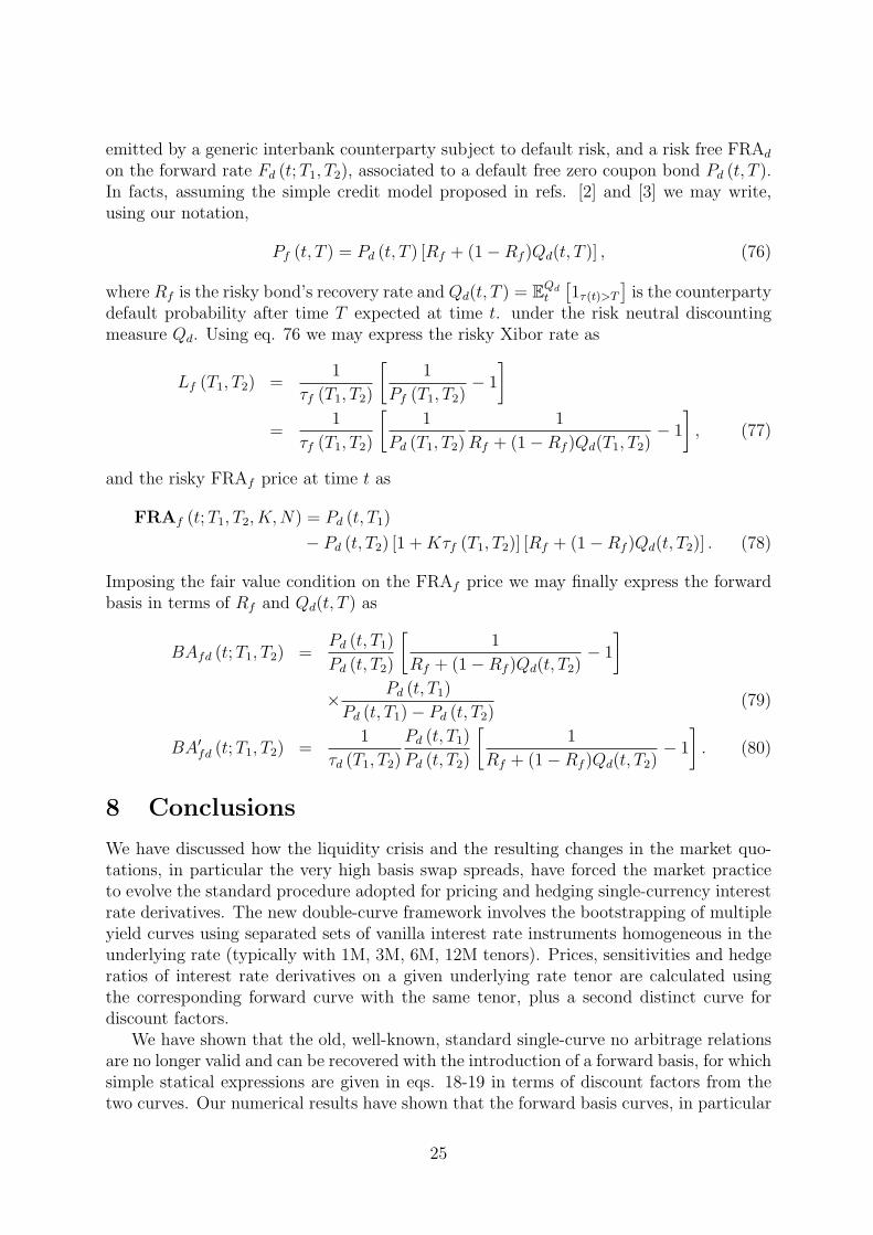
The credit crunch crisis started in the second half of 2007 has triggered, among many con-sequences, the explosion of the basis spreads quoted on the market between single-currencyinterest rate instruments, swaps in particular, characterised by different underlying ratetenors (e.g. Xibor3M 1, Xibor6M, etc.). In fig. 1 we show a snapshot of the marketquotations as of Feb. 16th, 2009 for the six basis swap term structures corresponding tothe four Euribor tenors 1M, 3M, 6M, 12M. As one can see, in the time interval 1Y − 30Ythe basis spreads are monotonically decreasing from 80 to around 2 basis points. Suchvery high basis reflect the higher liquidity risk suffered by financial institutions and thecorresponding preference for receiving payments with higher frequency (quarterly insteadof semi-annually, etc.).

1We denote with Xibor a generic Interbank Offered Rate. In the EUR case the Euribor is defined asthe rate at which euro interbank term deposits within the euro zone are offered by one prime bank toanother prime bank (see www.euribor.org).

2

EUR Basis swaps

0

10

20

30

40

50

60

70

80

1Y 2Y 3Y 4Y 5Y 6Y 7Y 8Y 9Y 10Y

11Y

12Y

15Y

20Y

25Y

30Y

bas

is s

pre

ad (

bp

s)

3M vs 6M1M vs 3M1M vs 6M6M vs 12M

3M vs 12M1M vs 12M

Figure 1: quotations (basis points) as of Feb. 16th, 2009 for the six EUR basis swapcurves corresponding to the four Euribor swap curves 1M, 3M, 6M, 12M. Before thecredit crunch of Aug. 2007 the basis spreads were just a few basis points (source: ReutersICAPEUROBASIS).

There are also other indicators of regime changes in the interest rate markets, such asthe divergence between deposit (Xibor based) and OIS 2 (Eonia3 based for EUR) rates,or between FRA4 contracts and the corresponding forward rates implied by consecutivedeposits (see e.g. refs. [1], [2], [3], [4]).

These frictions have thus induced a sort of “segmentation” of the interest rate marketinto sub-areas, mainly corresponding to instruments with 1M, 3M, 6M, 12M underlyingrate tenors, characterized, in principle, by different internal dynamics, liquidity and creditrisk premia, reflecting the different views and interests of the market players. Notice thatmarket segmentation was already present (and well understood) before the credit crunch(see e.g. ref. [5]), but not effective due to negligible basis spreads.

Such evolution of the financial markets has triggered a general reflection about themethodology used to price and hedge interest rate derivatives, namely those financialinstruments whose price depends on the present value of future interest rate-linked cash-flows. In this paper we acknowledge the current market practice, assuming the existenceof a given methodology (discussed in detail in ref. [1]) for bootstrapping multiple homoge-neous forwarding and discounting curves, characterized by different underlying rate tenors,and we focus on the consequences for pricing and hedging interest rate derivatives. In par-

2Overnight Indexed Swaps.3Euro OverNight Index Average, the rate computed as a weighted average of all overnight rates corre-

sponding to unsecured lending transactions in the euro-zone interbank market (see e.g. www.euribor.org).4Forward Rate Agreement.

3

ticular in sec. 3 we summarise the pre and post credit crunch market practices for pricingand hedging interest rate derivatives. In sec. 2 we fix the notation, we revisit some generalconcept of standard, no arbitrage single-curve pricing and we formalize the double-curvepricing framework, showing how no arbitrage is broken and can be formally recoveredwith the introduction of a forward basis. In sec. 5 we use the foreign-currency analogyto derive a single-currency version of the quanto adjustment, typical of cross-currencyderivatives, naturally appearing in the expectation of forward rates. In sec. 6 we derivethe no arbitrage double-curve market-like pricing expressions for basic single-currency in-terest rate derivatives, such as FRA, swaps, caps/floors and swaptions. Conclusions aresummarised in sec. 8.

The topic discussed here is a central problem in the interest rate market, with manyconsequences in trading, financial control, risk management and IT, which still lacks ofattention in the financial literature. To our knowledge, similar topics have been ap-proached in refs. [6], [7], [8], [2], [9]and [3], [4] . In particular W. Boenkost and W.Schmidt [7] discuss two methodologies for pricing cross-currency basis swaps, the first ofwhich (the actual pre-crisis common market practice), does coincide, once reduced to thesingle-currency case, with the double-curve pricing procedure described here5. RecentlyM. Kijima et al. [8] have extended the approach of ref. [7] to the (cross currency) caseof three curves for discount rates, Libor rates and bond rates. Finally, simultaneously tothe development of the present paper, M. Morini is approaching the problem in terms ofcounterparty risk [3], [4], F. Mercurio in terms of an extended Libor Market Model [2],and M. Henrard using an axiomatic model [9].

The present work follows an alternative route with respect to those cited above, in thesense that a) we adopt a bottom-up practitioner’s perspective, starting from the currentmarket practice of using multiple yield curves and working out its natural consequences,looking for a minimal and light generalisation of well-known frameworks, keeping thingsas simple as possible; b) we show how no-arbitrage can be recovered in the double-curveapproach by taking properly into account the forward basis, whose term structure canbe extracted from available basis swap market quotations; c) we use a straightforwardforeign-currency analogy to derive generalised double-curve market-like pricing expres-sions for basic single-currency interest rate derivatives, such as FRAs, swaps, caps/floorsand swaptions.

2 Notation and Basic Assumptions

Following the discussion above, we denote with Mx, x = d, f1, ..., fn multiple distinctinterest rate sub-markets, characterized by the same currency and by distinct bank ac-counts Bx and yield curves x in the form of a continuous term structure of discountfactors,

x = T −→ Px (t0, T ) , T ≥ t0 , (1)

5these authors were puzzled by the fact that their first methodology was neither arbitrage free nor con-sistent with the pre-crisis single-curve market practice for pricing single-currency swaps. Such objectionshave now been overcome by the market evolution towards a generalized double-curve pricing approach(see also [5]).

4

where t0 is the reference date of the curves (e.g. settlement date, or today) and Px (t, T )denotes the price at time t ≥ t0 of the Mx-zero coupon bond for maturity T , such thatPx (T, T ) = 1. In each sub-market Mx we postulate the usual no arbitrage relation,

Px (t, T2) = Px (t, T1)Px (t, T1, T2) , t ≤ T1 < T2 (2)

where Px (t, T1, T2) denotes the Mx forward discount factor from time T2 to time T1,prevailing at time t. The financial meaning of expression 2 is that, in each market Mx,given a cashflow of one unit of currency at time T2, its corresponding value at time t < T2

must be unique, both if we discount in one single step from T2 to t, using the discountfactor Px (t, T2), and if we discount in two steps, first from T2 to T1, using the forwarddiscount Px (t, T1, T2) and then from T1 to t, using Px (t, T1). Denoting with Fx (t;T1, T2)the simple compounded forward rate associated to Px (t, T1, T2), resetting at time T1 andcovering the time interval [T1;T2], we have

Px (t, T1, T2) =Px (t, T2)

Px (t, T1)=

1

1 + Fx (t;T1, T2) τx (T1, T2), (3)

where τx (T1, T2) is the year fraction between times T1 and T2 with daycount dcx, andfrom eq. 2 we obtain the familiar no arbitrage expression

Fx (t;T1, T2) =1

τx (T1, T2)

[1

Px (t, T1, T2)− 1

]=

Px (t, T1)− Px (t, T2)

τx (T1, T2)Px (t, T2). (4)

Eq. 4 can be also derived (see e.g. ref. [10], sec. 1.4) as the fair value condition at time tof the Forward Rate Agreement (FRA) contract with payoff at maturity T2 given by

FRAx (T2;T1, T2, K,N) = Nτx (T1, T2) [Lx (T1, T2)−K] , (5)

Lx (T1, T2) =1− Px (T1, T2)

τx (T1, T2)Px (T1, T2)(6)

where N is the nominal amount, Lx (T1, T2, dcx) is the T1-spot Xibor rate for maturity T2

and K the (simply compounded) strike rate (sharing the same daycount convention forsimplicity). Introducing expectations we have, ∀t ≤ T1 < T2,

FRAx (t;T1, T2, K,N) = Px (t, T2) EQT2x

t [FRA (T2;T1, T2, K,N)]

= NPx (t, T2) τx (T1, T2)

EQT2x

t [Lx (T1, T2)]−K

= NPx (t, T2) τx (T1, T2) [Fx (t;T1, T2)−K] , (7)

where QT2x denotes the Mx-T2-forward measure corresponding to the numeraire Px (t, T2),

EQt [.] denotes the expectation at time t w.r.t. measure Q and filtration Ft, encoding the

market information available up to time t, and we have assumed the standard martingaleproperty of forward rates

Fx (t;T1, T2) = EQT2x

t [Fx (T1;T1, T2)] = EQT2x

t [Lx (T1, T2)] (8)

to hold in each interest rate market Mx (see e.g. ref. [10]). We stress that the assumptionsabove imply that each sub-market Mx is internally consistent as the whole interest ratemarket before the crisis. This is surely a strong hypothesis, that could be relaxed in moresophisticated frameworks.

5

3 Pre and Post Credit Crunch Market Practices for

Pricing and Hedging Interest Rate Derivatives

We describe here the evolution of the market practice for pricing and hedging interestrate derivatives through the credit crunch crisis. We consider a general single-currencyinterest rate derivative with m future coupons with payoffs π = π1, ..., πm, with πi =πi (Fx), generating m cashflows c = c1, ..., cm at future dates T = T1, ..., Tm, witht < T1 < ... < Tm.

3.1 Single-Curve Framework

The pre-crisis standard market practice can be summarised in the following working pro-cedure (see e.g. refs. [11], [12], [13] and [14]):

1. select one finite set of the most convenient (i.e. liquid) interest rate vanilla instru-ments traded in real time on the market and build a single yield curve d usingthe preferred bootstrapping procedure; for instance, a common choice in the EURmarket is a combination of short-term EUR deposits, medium-term Futures/FRAon Euribor3M and medium-long-term swaps on Euribor6M;

2. for each interest rate coupon i ∈ 1, ...,m compute the relevant forward rates usingthe given yield curve d as in eq. 4,

Fd (t;Ti−1, Ti) =Pd (t, Ti−1)− Pd (t, Ti)

τd (Ti−1, Ti)Pd (t, Ti)t ≤ Ti−1 < Ti; (9)

3. compute cashflows ci as expectations at time t of the corresponding coupon payoffsπi (Fd) with respect to the Ti-forward measure QTi

d , associated to the numerairePd (t, Ti) from the same yield curve d,

ci = c (t, Ti, πi) = EQTid

t [πi (Fd)] ; (10)

4. compute the relevant discount factors Pd (t, Ti) from the same yield curve d;

5. compute the derivative’s price at time t as the sum of the discounted cashflows,

π (t; T) =m∑i=1

Pd (t, Ti) c (t, Ti, πi) =m∑i=1

Pd (t, Ti) EQTid

t [πi (Fd)] ; (11)

6. compute the delta sensitivity by shocking one by one the market pillars of yieldcurve d and hedge the resulting delta risk using the suggested amounts (hedgeratios) of the same set of vanillas.

For instance, a 5.5Y maturity EUR floating swap leg on Euribor1M (not directlyquoted on the market) is commonly priced using discount factors and forward rates cal-culated on the same depo-Futures-swap curve cited above. The corresponding delta riskis hedged using the suggested amounts (hedge ratios) of 5Y and 6Y Euribor6M swaps6.

6we refer here to the case of local yield curve bootstrapping methods, for which there is no sensitivitydelocalization effect (see refs. [12], [14]).

6

Notice that step 3 above has been formulated in terms of the pricing measure QTid

associated to the numeraire Pd (t, Ti). This is convenient in our context because it em-phasizes that the numeraire is associated to the discounting curve. Obviously any otherequivalent measure associated to different numeraires may be used as well.

We stress that this is a single-currency-single-curve approach, in that a unique yieldcurve is built and used to price and hedge any interest rate derivative on a given currency.Thinking in terms of more fundamental variables, e.g. the short rate, this is equivalent toassume that there exist a unique fundamental underlying short rate process able to modeland explain the whole term structure of interest rates of all tenors. It is also a relativepricing approach, because both the price and the hedge of a derivative are calculatedrelatively to a set of vanillas quoted on the market. We notice also that it is not strictlyguaranteed to be arbitrage-free, because discount factors and forward rates obtained froma given yield curve through interpolation are, in general, not necessarily consistent withthose obtained by a no arbitrage model; in practice bid-ask spreads and transaction costshide any arbitrage possibilities. Finally, we stress that the key first point in the procedureis much more a matter of art than of science, because there is not an unique financiallysound recipe for selecting the bootstrapping instruments and rules.

3.2 Multiple-Curve Framework

Unfortunately, the pre-crisis approach outlined above is no longer consistent, at least inits simple formulation, with the present market conditions. First, it does not take intoaccount the market information carried by basis swap spreads, now much larger thanin the past and no longer negligible. Second, it does not take into account that theinterest rate market is segmented into sub-areas corresponding to instruments with dis-tinct underlying rate tenors, characterized, in principle, by different dynamics (e.g. shortrate processes). Thus, pricing and hedging an interest rate derivative on a single yieldcurve mixing different underlying rate tenors can lead to “dirty” results, incorporating thedifferent dynamics, and eventually the inconsistencies, of distinct market areas, makingprices and hedge ratios less stable and more difficult to interpret. On the other side, themore the vanillas and the derivative share the same homogeneous underlying rate, thebetter should be the relative pricing and the hedging. Third, by no arbitrage, discountingmust be unique: two identical future cashflows of whatever origin must display the samepresent value; hence we need a unique discounting curve.

In principle, a consistent credit and liquidity theory would be required to account forthe interest rate market segmentation. This would also explain the reason why the asym-metries cited above do not necessarily lead to arbitrage opportunities, once counterpartyand liquidity risks are taken into account. Unfortunately such a framework is not easy toconstruct (see e.g. the discussion in refs. [2], [4]). In practice an empirical approach hasprevailed on the market, based on the construction of multiple “forwarding” yield curvesfrom plain vanilla market instruments homogeneous in the underlying rate tenor, used tocalculate future cash flows based on forward interest rates with the corresponding tenor,and of a single “discounting” yield curve, used to calculate discount factors and cash flows’present values. Consequently, interest rate derivatives with a given underlying rate tenorshould be priced and hedged using vanilla interest rate market instruments with the sameunderlying rate tenor. The post-crisis market practice may thus be summarised in the

7

following working procedure:

1. build one discounting curve d using the preferred selection of vanilla interest ratemarket instruments and bootstrapping procedure;

2. build multiple distinct forwarding curves f1 , ..., fn using the preferred selectionsof distinct sets of vanilla interest rate market instruments, each homogeneous inthe underlying Xibor rate tenor (typically with 1M, 3M, 6M, 12M tenors) andbootstrapping procedures;

3. for each interest rate coupon i ∈ 1, ...,m compute the relevant forward rates withtenor f using the corresponding yield curve f as in eq. 4,

Ff (t;Ti−1, Ti) =Pf (t, Ti−1)− Pf (t, Ti)

τf (Ti−1, Ti)Pf (t, Ti), t ≤ Ti−1 < Ti; (12)

4. compute cashflows ci as expectations at time t of the corresponding coupon payoffsπi (Ff ) with respect to the discounting Ti-forward measure QTi

d , associated to thenumeraire Pd (t, Ti), as

ci = c (t, Ti, πi) = EQTid

t [πi (Ff )] ; (13)

5. compute the relevant discount factors Pd (t, Ti) from the discounting yield curve d;

6. compute the derivative’s price at time t as the sum of the discounted cashflows,

π (t; T) =m∑i=1

Pd (t, Ti) c (t, Ti, πi) =m∑i=1

Pd (t, Ti) EQTid

t [πi (Ff )] ; (14)

7. compute the delta sensitivity by shocking one by one the market pillars of each yieldcurve d, f1 , ..., fn and hedge the resulting delta risk using the suggested amounts(hedge ratios) of the corresponding set of vanillas.

For instance, the 5.5Y floating swap leg cited in the previous section 3.1 is currentlypriced using Euribor1M forward rates calculated on the 1M forwarding curve, boot-strapped using Euribor1M vanillas only, plus discount factors calculated on the discount-ing curve d. The delta sensitivity is computed by shocking one by one the market pillarsof both 1M and d curves and the resulting delta risk is hedged using the suggestedamounts (hedge ratios) of 5Y and 6Y Euribor1M swaps plus the suggested amounts of5Y and 6Y instruments from the discounting curve d (see sec. 6.2 for more details aboutthe hedging procedure).

Such multiple-curve framework is consistent with the present market situation, but -there is no free lunch - it is also more demanding. First, the discounting curve clearly playsa special and fundamental role, and must be built with particular care. This “pre-crisis”obvious step has become, in the present market situation, a very subtle and controversialpoint, that would require a whole paper in itself (see e.g. ref. [15]). In fact, while theforwarding curves construction is driven by the underlying rate homogeneity principle, for

8

which there is (now) a general market consensus, there is no longer, at the moment, generalconsensus for the discounting curve construction. At least two different practices can beencountered in the market: a) the old “pre-crisis” approach (e.g. the depo, Futures/FRAand swap curve cited before), that can be justified with the principle of maximum liquid-ity (plus a little of inertia), and b) the OIS curve, based on the overnight rate7 (Eoniafor EUR), justified with collateralized (riskless) counterparties8 (see e.g. refs. [16], [17]).Second, building multiple curves requires multiple quotations: many more bootstrappinginstruments must be considered (deposits, Futures, swaps, basis swaps, FRAs, etc., ondifferent underlying rate tenors), which are available on the market with different degreesof liquidity and can display transitory inconsistencies (see [1]). Third, non trivial inter-polation algorithms are crucial to produce smooth forward curves (see e.g. refs. [12]-[14],[1]). Fourth, multiple bootstrapping instruments implies multiple sensitivities, so hedg-ing becomes more complicated. Last but not least, pricing libraries, platforms, reports,etc. must be extended, configured, tested and released to manage multiple and separatedyield curves for forwarding and discounting, not a trivial task for quants, risk managers,developers and IT people.

The static multiple-curve pricing & hedging methodology described above can be ex-tended, in principle, by adopting multiple distinct models for the evolution of the underly-ing interest rates with tenors f1, ..., fn to calculate the future dynamics of the yield curvesf1 , ..., fn and the expected cashflows. The volatility/correlation dependencies carriedby such models imply, in principle, bootstrapping multiple distinct variance/covariancematrices and hedging the corresponding sensitivities using volatility- and correlation-dependent vanilla market instruments. Such more general approach has been carried onin ref. [2] in the context of generalised market models. In this paper we will focus only onthe basic matter of static yield curves and leave out the dynamical volatility/correlationdimensions.

4 No Arbitrage and Forward Basis

Now, we wish to understand the consequences of the assumptions above in terms of noarbitrage. First, we notice that in the multiple-curve framework classic single-curve noarbitrage relations such as eq. 4 are broken up, being

Pf (t, T1, T2) =Pf (t, T2)

Pf (t, T1)=

1

1 + Ff (t;T1, T2) τf (T1, T2)

6= 1

1 + Fd (t;T1, T2) τd (T1, T2)=Pd (t, T2)

Pd (t, T1)= Pd (t, T1, T2) . (15)

No arbitrage between distinct yield curves d and f can be immediately recovered bytaking into account the forward basis, the forward counterparty of the quoted market

7the overnight rate can be seen as the best proxy to a risk free rate available on the market becauseof its 1-day tenor.

8collateral agreements are more and more used in OTC markets, where there are no clearing houses,to reduce the counterparty risk. The standard ISDA contracts (ISDA Master Agreement and CreditSupport Annex) include netting clauses imposing compensation. The compensation frequency is oftenon a daily basis and the (cash or asset) compensation amount is remunerated at overnight rate.

9

basis of fig. 1, defined as

Pf (t, T1, T2) :=1

1 + Fd (t;T1, T2)BAfd (t, T1, T2) τd (T1, T2), (16)

or through the equivalent simple transformation rule for forward rates

Ff (t;T1, T2) τf (T1, T2) = Fd (t;T1, T2) τd (T1, T2)BAfd (t, T1, T2) . (17)

From eq. 17 we can express the forward basis as a ratio between forward rates or, equiv-alently, in terms of discount factors from d and f curves as

BAfd (t, T1, T2) =Ff (t;T1, T2) τf (T1, T2)

Fd (t;T1, T2) τd (T1, T2)

=Pd (t, T2)

Pf (t, T2)

Pf (t, T1)− Pf (t, T2)

Pd (t, T1)− Pd (t, T2). (18)

Obviously the following alternative additive definition is completely equivalent

Pf (t, T1, T2) : =1

1 +[Fd (t;T1, T2) +BA′fd (t, T1, T2)

]τd (T1, T2)

,

BA′fd (t, T1, T2) =Ff (t;T1, T2) τf (T1, T2)− Fd (t;T1, T2) τd (T1, T2)

τd (T1, T2)

=1

τd (T1, T2)

[Pf (t, T1)

Pf (t, T2)− Pd (t, T1)

Pd (t, T2)

]= Fd (t;T1, T2) [BAfd (t, T1, T2)− 1] , (19)

which is more useful for comparisons with the market basis spreads of fig. 1. Notice thatif d = f we recover the single-curve case BAfd (t, T1, T2) = 1, BA′fd (t, T1, T2) = 0.

We stress that the forward basis in eqs. 18-19 is a straightforward consequence ofthe assumptions above, essentially the existence of two yield curves and no arbitrage. Itsadvantage is that it allows for a direct computation of the forward basis between forwardrates for any time interval [T1, T2], which is the relevant quantity for pricing and hedginginterest rate derivatives. In practice its value depends on the market basis spread betweenthe quotations of the two sets of vanilla instruments used in the bootstrapping of the twocurves d and f . On the other side, the limit of expressions 18-19 is that they reflectthe statical9 differences between the two interest rate markets Md, Mf carried by the twocurves d, f , but they are completely independent of the interest rate dynamics in Md

and Mf .Notice also that the approach can be inverted to bootstrap a new yield curve from a

9we remind that the discount factors in eqs. 18-18 are calculated on the curves d, f following therecipe described in sec. 3.2, not using any dynamical model for the evolution of the rates.

10

given yield curve plus a given forward basis, using the following recursive relations

Pd,i =Pf,iBAfd,i

Pf,i−1 − Pf,i + Pf,iBAfd,iPd,i−1

=Pf,i

Pf,i−1 − Pf,iBA′fd,iτd,iPd,i−1, (20)

Pf,i =Pd,i

Pd,i + (Pd,i−1 − Pd,i)BAfd,iPf,i−1

=Pd,i

Pd,i + Pd,i−1BA′fd,iτd,iPf,i−1, (21)

where we have inverted eqs. 18, 19 and shortened the notation by putting τx (Ti−1, Ti) :=τx,i, Px (t, Ti) := Px,i, BAfd (t, Ti−1, Ti) := BAfd,i. Given the yield curve x up to stepPx,i−1 plus the forward basis for the step i − 1 → i, the equations above can be used toobtain the next step Px,i.

We now discuss a numerical example of the forward basis in a realistic market situation.We consider the four interest rate underlyings I = I1M , I3M , I6M , I12M, where I =Euribor index, and we bootstrap from market data five distinct yield curves = d,1M , 3M , 6M , 12M, using the first one for discounting and the others for forwarding.We follow the methodology described in ref. [1] using the corresponding open-sourcedevelopment available in the QuantLib framework [18]. The discounting curve d is builtfollowing a “pre-crisis” traditional recipe from the most liquid deposit, IMM Futures/FRAon Euribor3M and swaps on Euribor6M. The other four forwarding curves are built fromconvenient selections of depos, FRAs, Futures, swaps and basis swaps with homogeneousunderlying rate tenors; a smooth and robust algorithm (monotonic cubic spline on logdiscounts) is used for interpolations. Different choices (e.g. an Eonia discounting curve)as well as other technicalities of the bootstrapping described in ref. [1] obviously wouldlead to slightly different numerical results, but do not alter the conclusions drawn here.

In fig. 2 we plot both the 3M-tenor forward rates and the zero rates calculated on dand 3M as of 16th Feb. 2009 cob10. Similar patterns are observed also in the other 1M,3M, 12M curves (not shown here, see ref. [1]). In fig. 3 (upper panels) we plot the termstructure of the four corresponding multiplicative forward basis curves f − d calculatedthrough eq. 18. In the lower panels we also plot the additive forward basis given by eq.19. We observe in particular that the higher short-term basis adjustments (left panels)are due to the higher short-term market basis spreads (see fig. 1). Furthermore, themedium-long-term 6M − d basis (dash-dotted green lines in the right panels) are closeto 1 and 0, respectively, as expected from the common use of 6M swaps in the two curves.A similar, but less evident, behavior is found in the short-term 3M −d basis (continuousblue line in the left panels), as expected from the common 3M Futures and the uncommondeposits. The two remaining basis curves 1M − d and 12M − d are generally far from1 or 0 because of different bootstrapping instruments. Obviously such details depend onour arbitrary choice of the discounting curve.

Overall, we notice that all the basis curves f − d reveal a complex micro-term struc-ture, not present either in the monotonic basis swaps market quotes of fig. 1 or in the

10close of business.

11

EUR discounting curve

1.0%

1.5%

2.0%

2.5%

3.0%

3.5%

4.0%

4.5%

5.0%

Fe

b 0

9

Fe

b 1

2

Fe

b 1

5

Fe

b 1

8

Fe

b 2

1

Fe

b 2

4

Fe

b 2

7

Fe

b 3

0

Fe

b 3

3

Fe

b 3

6

Fe

b 3

9

Zero rates

Forward rates

EUR forwarding curve 3M

1.0%

1.5%

2.0%

2.5%

3.0%

3.5%

4.0%

4.5%

5.0%

Fe

b 0

9

Fe

b 1

2

Fe

b 1

5

Fe

b 1

8

Fe

b 2

1

Fe

b 2

4

Fe

b 2

7

Fe

b 3

0

Fe

b 3

3

Fe

b 3

6

Fe

b 3

9

Zero rates

Forward rates

Figure 2: EUR discounting curve d (upper panel) and 3M forwarding curve 3Mf

(lower panel) at end of day Feb. 16th 2009. Blue lines: 3M-tenor forward ratesF (t0; t, t+ 3M, act/360 ), t daily sampled and spot date t0 = 18th Feb. 2009; red lines:zero rates F (t0; t, act/365 ). Similar patterns are observed also in the 1M, 6M, 12M curves(not shown here, see ref. [1]).

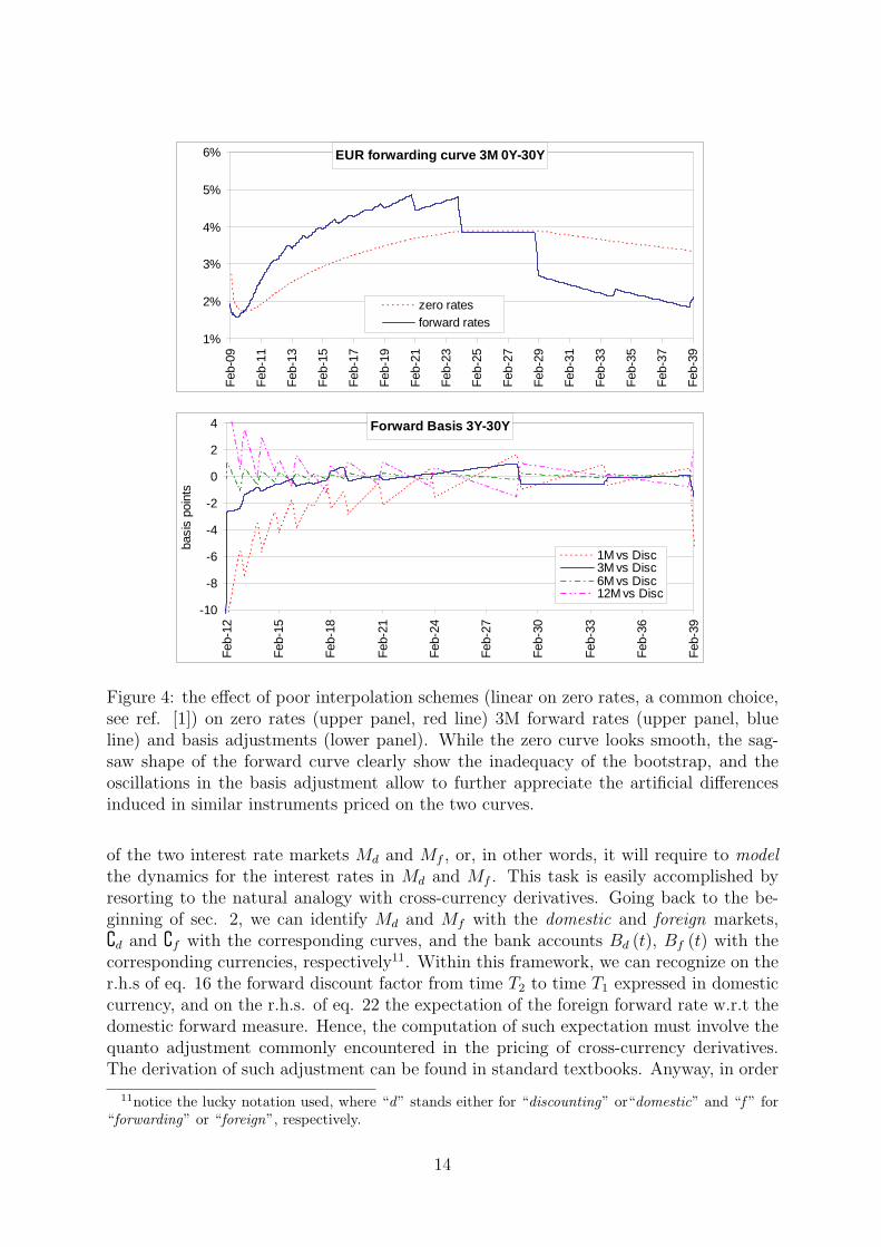
smooth yield curves x. Such effect is essentially due to an amplification mechanism ofsmall local differences between the d and f forward curves. In fig. 4 we also showthat smooth yield curves are a crucial input for the forward basis: using a non-smoothbootstrapping (linear interpolation on zero rates, still a diffused market practice), thezero curve apparently shows no particular problems, while the forward curve displays asagsaw shape inducing, in turn, strong and unnatural oscillations in the forward basis.

We conclude that, once a smooth and robust bootstrapping technique for yield curveconstruction is used, the richer term structure of the forward basis curves provides asensitive indicator of the tiny, but observable, statical differences between different interestrate market sub-areas in the post credit crunch interest rate world, and a tool to assess thedegree of liquidity and credit issues in interest rate derivatives’ prices. It is also helpful fora better explanation of the profit&loss encountered when switching between the single-and the multiple-curve worlds.

12

Forward Basis (additive)

-60

-40

-20

0

20

40

60

80

Feb

-09

May

-09

Aug

-09

Nov

-09

Feb

-10

May

-10

Aug

-10

Nov

-10

Feb

-11

May

-11

Aug

-11

Nov

-11

Feb

-12

basi

s po

ints

1M vs Disc3M vs Disc6M vs Disc12M vs Disc

Forward Basis (additive)

-7

-5

-3

-1

1

3

5

7

Feb

-12

Feb

-15

Feb

-18

Feb

-21

Feb

-24

Feb

-27

Feb

-30

Feb

-33

Feb

-36

Feb

-39

basi

s po

ints

1M vs Disc3M vs Disc6M vs Disc12M vs Disc

Forward Basis (multiplicative)

0.7

0.8

0.9

1.0

1.1

1.2

1.3

1.4

1.5

1.6F

eb-0

9

May

-09

Aug

-09

Nov

-09

Feb

-10

May

-10

Aug

-10

Nov

-10

Feb

-11

May

-11

Aug

-11

Nov

-11

Feb

-12

1M vs Disc3M vs Disc6M vs Disc12M vs Disc

Forward Basis (multiplicative)

0.98

0.99

1.00

1.01

1.02

Feb

-12

Feb

-15

Feb

-18

Feb

-21

Feb

-24

Feb

-27

Feb

-30

Feb

-33

Feb

-36

Feb

-39

1M vs Disc3M vs Disc6M vs Disc12M vs Disc

Figure 3: upper panels: multiplicative basis adjustments from eq. 18 as of end of dayFeb. 16th, 2009, for daily sampled 3M-tenor forward rates as in fig. 2, calculated on I1M

f ,

I3Mf , I6M

f and I12Mf curves against d taken as reference curve. Lower panels: equivalent

plots of the additive basis adjustment of eq. 19 between the same forward rates (basispoints). Left panels: 0Y-3Y data; Right panels: 3Y-30Y data on magnified scales. Thehigher short-term adjustments seen in the left panels are due to the higher short-termmarket basis spread (see Figs. 1). The oscillating term structure observed is due to theamplification of small differences in the term structures of the curves.

5 Foreign-Currency Analogy and Quanto Adjustment

A second important issue regarding no-arbitrage arises in the multiple-curve framework.From eq. 13 we have that, for instance, the single-curve FRA price in eq. 7 is generalisedinto the following multiple-curve expression

FRA (t;T1, T2, K,N) = NPd (t, T2) τf (T1, T2)

EQ

T2d

t [Lf (T1, T2)]−K. (22)

Instead, the current market practice is to price such FRA simply as

FRA (t;T1, T2, K,N) ' NPd (t, T2) τf (T1, T2) [Ff (t;T1, T2)−K] . (23)

Obviously the forward rate Ff (t;T1, T2) is not, in general, a martingale under the discount-ing measure QT2

d , so eq. 23 discards the adjustment coming from this measure mismatch.Hence, a theoretically correct pricing within the multiple-curve framework requires thecomputation of expectations as in eq. 22 above. This will involve the dynamic properties

13

EUR forwarding curve 3M 0Y-30Y

1%

2%

3%

4%

5%

6%

Feb

-09

Feb

-11

Feb

-13

Feb

-15

Feb

-17

Feb

-19

Feb

-21

Feb

-23

Feb

-25

Feb

-27

Feb

-29

Feb

-31

Feb

-33

Feb

-35

Feb

-37

Feb

-39

zero ratesforward rates

Forward Basis 3Y-30Y

-10

-8

-6

-4

-2

0

2

4

Feb

-12

Feb

-15

Feb

-18

Feb

-21

Feb

-24

Feb

-27

Feb

-30

Feb

-33

Feb

-36

Feb

-39

basi

s po

ints

1M vs Disc3M vs Disc6M vs Disc12M vs Disc

Figure 4: the effect of poor interpolation schemes (linear on zero rates, a common choice,see ref. [1]) on zero rates (upper panel, red line) 3M forward rates (upper panel, blueline) and basis adjustments (lower panel). While the zero curve looks smooth, the sag-saw shape of the forward curve clearly show the inadequacy of the bootstrap, and theoscillations in the basis adjustment allow to further appreciate the artificial differencesinduced in similar instruments priced on the two curves.

of the two interest rate markets Md and Mf , or, in other words, it will require to modelthe dynamics for the interest rates in Md and Mf . This task is easily accomplished byresorting to the natural analogy with cross-currency derivatives. Going back to the be-ginning of sec. 2, we can identify Md and Mf with the domestic and foreign markets,d and f with the corresponding curves, and the bank accounts Bd (t), Bf (t) with thecorresponding currencies, respectively11. Within this framework, we can recognize on ther.h.s of eq. 16 the forward discount factor from time T2 to time T1 expressed in domesticcurrency, and on the r.h.s. of eq. 22 the expectation of the foreign forward rate w.r.t thedomestic forward measure. Hence, the computation of such expectation must involve thequanto adjustment commonly encountered in the pricing of cross-currency derivatives.The derivation of such adjustment can be found in standard textbooks. Anyway, in order

11notice the lucky notation used, where “d” stands either for “discounting” or“domestic” and “f ” for“forwarding” or “foreign”, respectively.

14

to fully appreciate the parallel with the present double-curve-single-currency case, it isuseful to run through it once again. In particular, we will adapt to the present contextthe discussion found in ref. [10], chs. 2.9 and 14.4.

5.1 Forward Rates

In the double–curve-double-currency case, no arbitrage requires the existence at any timet0 ≤ t ≤ T of a spot and a forward exchange rate between equivalent amounts of moneyin the two currencies such that

cd (t) = xfd (t) cf (t) , (24)

Xfd (t, T )Pd (t, T ) = xfd (t)Pf (t, T ) , (25)

where the subscripts f and d stand for foreign and domestic, cd (t) is any cashflow (amountof money) at time t in units of domestic-currency and cf (t) is the corresponding cashflowat time t (the corresponding amount of money) in units of foreign currency. ObviouslyXfd (t, T )→ xfd (t) for t→ T . Expression 25 is still a consequence of no arbitrage. Thiscan be understood with the aid of fig. 5: starting from top right corner in the time vscurrency/yield curve plane with an unitary cashflow at time T > t in foreign currency,we can either move along path A by discounting at time t on curve f using Pf (t, T ) andthen by changing into domestic currency units using the spot exchange rate xfd (t), endingup with xfd (t)Pf (t, T ) units of domestic currency; or, alternatively, we can follow pathB by changing at time T into domestic currency units using the forward exchange rateXfd (t, T ) and then by discounting on d using Pd (t, T ), ending up with Xfd (t, T )Pd (t, T )units of domestic currency. Both paths stop at bottom left corner, hence eq. 25 musthold by no arbitrage.

Now, our double-curve-single-currency case is immediately obtained from the discus-sion above by thinking to the subscripts f and d as shorthands for forwarding and dis-counting and by recognizing that, having a single currency, the spot exchange rate mustcollapse to 1. We thus have

xfd (t) = 1, (26)

Xfd (t, T ) =Pf (t, T )

Pd (t, T ). (27)

Obviously for d = f we recover the single-currency, single-curve case Xfd (t, T ) = 1 ∀t, T . The interpretation of the forward exchange rate in eq. 27 within this framework isstraightforward: it is nothing else that the counterparty of the forward basis in eq. 17 fordiscount factors on the two yield curves d and f . Substituting eq. 27 into eq. 17 weobtain the following relation

BAfd (t, T1, T2) = Xfd (t, T2)τf (T1, T2)

τd (T1, T2)

× Pd (t, T1)− Pd (t, T2)

Pd (t, T1)Xfd (t, T1)− Pd (t, T2)Xfd (t, T1). (28)

Notice that we could forget the foreign currency analogy above and start by postulatingXfd (t, T ) as in eq. 27, name it forward basis and proceed with the next step.

15

Figure 5: Picture of no-arbitrage interpretation for the forward exchange rate in eq. 25.Moving, in the yield curve vs time plane, from top right to bottom left corner throughpath A or path B must be equivalent. Alternatively, we may think to no-arbitrage as asort of zero “circuitation”, sum of all trading events following a closed path starting andstopping at the same point in the plane. This description is equivalent to the traditional“table of transaction” picture, as found e.g. in fig. 1 of ref. [5].

We proceed by assuming, according to the standard market practice, the following(driftless) lognormal martingale dynamic for f (foreign) forward rates

dFf (t;T1, T2)

Ff (t;T1, T2)= σf (t) dW T2

f (t) , t ≤ T1, (29)

where σf (t) is the volatility (positive deterministic function of time) of the process, un-

der the probability space(Ω,Ff , QT2

f

)with the filtration Fft generated by the brownian

motion W T2f under the forwarding (foreign) T2−forward measure QT2

f , associated to the

f (foreign) numeraire Pf (t, T2).Next, since Xfd (t, T2) in eq. 27 is the ratio between the price at time t of a d

(domestic) tradable asset (xfd (t)Pf (t, T2) in eq. 25, or Pf (t, T2) in eq. 27 with xfd (t) =1) and the D numeraire Pd (t, T2), it must evolve according to a (driftless) martingaleprocess under the associated discounting (domestic) T2−forward measure QT2

d ,

dXfd (t, T2)

Xfd (t, T2)= σX (t) dW T2

X (t) , t ≤ T2, (30)

16

where σX (t) is the volatility (positive deterministic function of time) of the process andW T2X is a brownian motion under QT2

d such that

dW T2f (t) dW T2

X (t) = ρfX (t) dt. (31)

Now, in order to calculate expectations such as in the r.h.s. of eq. 22, we must switchfrom the forwarding (foreign) measure QT2

f associated to the numeraire Pf (t, T2) to the

discounting (domestic) measure QT2d associated to the numeraire Pd (t, T2). In our double-

curve-single-currency language this amounts to transform a cashflow on curve f to thecorresponding cashflow on curve d. Recurring to the change-of-numeraire technique (seerefs. [10], [19], [20]) we obtain that the dynamic of Ff (t;T1, T2) under QT2

d acquires anon-zero drift

dFf (t;T1, T2)

Ff (t;T1, T2)= µf (t) dt+ σf (t) dW T2

f (t) , t ≤ T1, (32)

µf (t) = −σf (t)σX (t) ρfX (t) , (33)

and that Ff (T1;T1, T2) is lognormally distributed under QT2d with mean and variance given

by

EQT2d

t

[lnFf (T1;T1, T2)

Ff (t;T1, T2)

]=

∫ T1

t

[µf (u)− 1

2σ2f (u)

]du, (34)

VarQ

T2d

t

[lnFf (T1;T1, T2)

Ff (t;T1, T2)

]=

∫ T1

t

σ2f (u) du. (35)

We thus obtain the following expressions, for t0 ≤ t < T1,

EQT2d

t [Ff (T1;T1, T2)] = Ff (t;T1, T2)QAfd (t, T1, σf , σX , ρfX) , (36)

QAfd (t, T1, σf , σX , ρfX) = exp

∫ T1

t

µf (u) du

= exp

[−∫ T1

t

σf (u)σX (u) ρfX (u) du

], (37)

where QAfd (t, T1, σf , σX , ρfX) is the (multiplicative) quanto adjustment. We may alsodefine an additive quanto adjustment as

EQT2d

t [Ff (T1;T1, T2)] = Ff (t;T1, T2) +QA′fd (t, T1, σf , σX , ρfX) , (38)

QA′fd (t, T1, σf , σX , ρfX) = Ff (t;T1, T2) [QAfd (t, T1, σf , σX , ρfX)− 1] , (39)

where the second relation comes from eq. 36. Finally, combining eqs. 36, 38 with eqs.18, 19 we may derive a relation between the quanto and the basis adjustments,

BAfd (t, T1, T2)

QAfd (t, T1, σf , σX , ρfX)=

EQT2d

t [Ld (T1, T2)]

EQT2d

t [Lf (T1, T2)], (40)

BA′fd (t, T1, T2)−QA′fd (t, T1, σf , σX , ρfX) = EQT2d

t [Ld (T1, T2)]− EQT2d

t [Lf (T1, T2)] (41)

17

for multiplicative and additive adjustments, respectively.We conclude that the foreign-currency analogy allows us to compute the expectation

in eq. 22 of a forward rate on curve f w.r.t. the discounting measure QT2d in terms of

a well-known quanto adjustment, typical of cross-currency derivatives. Such adjustmentnaturally follows from a change between the T -forward probability measures QT2

f and

QT2d , or numeraires Pf (t, T2) and Pd (t, T2), associated to the two yield curves, f and

d, respectively. Notice that the expression 37 depends on the average over the timeinterval [t, T1] of the product of the volatility σf of the f (foreign) forward rates Ff , ofthe volatility σX of the forward exchange rate Xfd between curves f and d, and of thecorrelation ρfX between Ff and Xfd. It does not depend either on the volatility σd of thed (domestic) forward rates Fd or on any stochastic quantity after time T1. The latter factis actually quite natural, because the stochasticity of the forward rates involved ceases attheir fixing time T1. The dependence on the cashflow time T2 is actually implicit in eq37, because the volatilities and the correlation involved are exactly those of the forwardand exchange rates on the time interval [T1, T2]. Notice in particular that a non-trivialadjustment is obtained if and only if the forward exchange rate Xfd is stochastic (σX 6= 0)and correlated to the forward rate Ff (ρfX 6= 0); otherwise expression 37 collapses to thesingle curve case QAfd = 1.

The volatilities and the correlation in eq. 37 can be extracted from market data.In the EUR market the volatility σf can be extracted from quoted cap/floor options onEuribor6M, while for other rate tenors and for σX and ρfX one must resort to historicalestimates. Conversely, given a forward basis term structure, such that in fig. 3, one couldtake σf from the market, assume for simplicity ρfX ' 1 (or any other functional form), andbootstrap out a term structure for the forward exchange rate volatility σX . Notice that inthis way we are also able to compare information about the internal dynamics of differentmarket sub-areas. We will give some numerical estimate of the quanto adjustment in thenext section 6.

5.2 Swap Rates

The discussion above can be remapped, with some attention, to swap rates. Given twoincreasing dates sets T = T0, ..., Tn, S = S0, ..., Sm, T0 = S0 ≥ t and an interestrate swap with a floating leg paying at times Ti, i = 1, .., n, the Xibor rate with tenor[Ti−1, Ti] fixed at time Ti−1, plus a fixed leg paying at times Sj, j = 1, ..,m, a fixedrate, the corresponding fair swap rate Sf (t,T,S) on curve f is defined by the followingequilibrium (no arbitrage) relation between the present values of the two legs,

Sf (t,T,S)Af (t,S) =n∑i=1

Pf (t, Ti) τf (Ti−1, Ti)Ff (t;Ti−1, Ti) , t ≤ T0 = S0, (42)

where

Af (t,S) =m∑j=1

Pf (t, Sj) τf (Sj−1, Sj) (43)

is the annuity on curve f . Following the standard market practice, we observe that,assuming the annuity as the numeraire on curve f , the swap rate in eq. 42 is the

18

ratio between a tradable asset (the value of the swap floating leg on curve f ) and thenumeraire Af (t,S), and thus it is a martingale under the associated forwarding (foreign)swap measure QS

f . Hence we can assume, as in eq. 29, a driftless geometric brownian

motion for the swap rate under QSf ,

dSf (t,T,S)

Sf (t,T,S)= νf (t,T,S) dWT,S

f (t) , t ≤ T0, (44)

where υf (t,T,S) is the volatility (positive deterministic function of time) of the process

and WT,Sf is a brownian motion under QS

f . Then, mimicking the discussion leading toeqs. 26-27, the following relation

m∑j=1

Pd (t, Sj) τd (Sj−1, Sj)Xfd (t, Sj) = xfd (t)m∑j=1

Pf (t, Sj) τf (Sj−1, Sj)

= Af (t,S) (45)

must hold by no arbitrage between the two curves f and d. Defining a swap forwardexchange rate Yfd (t,S) such that

Af (t,S) , =m∑j=1

Pd (t, Sj) τd (Sj−1, Sj)Xfd (t, Sj)

= Yfd (t,S)m∑j=1

Pd (t, Sj) τd (Sj−1, Sj) = Yfd (t,S)Ad (t,S) , (46)

we obtain the expression

Yfd (t,S) =Af (t,S)

Ad (t,S), (47)

equivalent to eq. 27. Hence, since Yfd (t,S) is the ratio between the price at time t of thed (domestic) tradable asset xfd (t)Af (t,S) and the numeraire Ad (t,S), it must evolveaccording to a (driftless) martingale process under the associated discounting (domestic)swap measure QS

d ,dYfd (t,S)

Yfd (t,S)= νY (t,S) dWS

Y (t) , t ≤ T0, (48)

where vY (t,S) is the volatility (positive deterministic function of time) of the process andWSY is a brownian motion under QS

d such that

dWT,Sf (t) dWS

Y (t) = ρfY (t,T,S) dt. (49)

Now, applying again the change-of-numeraire technique of sec. 5.1, we obtain that thedynamic of the swap rate Sf (t,T,S) under the discounting (domestic) swap measure QS

d

acquires a non-zero drift

dSf (t,T,S)

Sf (t,T,S)= λf (t,T,S) dt+ νf (t,T,S) dWT,S

f (t) , t ≤ T0, (50)

λf (t,T,S) = −νf (t,T,S) νY (t,S) ρfY (t,T,S) , (51)

19

and that Sf (t,T,S) is lognormally distributed under QSd with mean and variance given

by

EQSd

t

[lnSf (T0,T,S)

Sf (t,T,S)

]=

∫ T0

t

[λf (u,T,S)− 1

2ν2f (u,T,S)

]du, (52)

VarQS

dt

[lnSf (T0,T,S)

Sf (t,T,S)

]=

∫ T0

tf

ν2f (u,T,S) du. (53)

We thus obtain the following expressions, for t0 ≤ t < T0,

EQSd

t [Sf (T0,T,S)] = Sf (t,T,S)QAfd (t,T,S, νf , νY , ρfY ) , (54)

QAfd (t,T,S, νf , νY , ρfY ) = exp

∫ T0

t

λf (u,T,S) du

= exp

[−∫ T0

t

νf (u,T,S) νY (u,S) ρfY (u,T,S) du

](55)

The same considerations as in sec. 5.1 apply. In particular, we observe that the ad-justment in eqs. 54, 56 naturally follows from a change between the probability measuresQSf and QS

d , or numeraires Af (t,S) and Ad (t,S), associated to the two yield curves, fand d, respectively, once swap rates are considered. In the EUR market, the volatilityνf (u,T,S) in eq. 55 can be extracted from quoted swaptions on Euribor6M, while forother rate tenors and for νY (u,S) and ρfY (u,T,S) one must resort to historical estimates.

An additive quanto adjustment can also be defined as before

EQSd

t [Sf (T0,T,S)] = Sf (t,T,S) +QA′fd (t,T,S, νf , νY , ρfY ) , (56)

QA′fd (t,T,S, νf , νY , ρfY ) = Sf (t,T,S) [QAfd (t,T,S, νf , νY , ρfY )− 1] . (57)

6 Double-Curve Pricing & Hedging Interest Rate Deriva-

tives

6.1 Pricing

The results of sec. 5 above allows us to derive no arbitrage, double-curve-single-currencypricing formulas for interest rate derivatives. The recipes are, basically, eqs. 36-37 or54-55.

The simplest interest rate derivative is a floating zero coupon bond paying at time Ta single cashflow depending on a single spot rate (e.g. the Xibor) fixed at time t < T ,

ZCB (T ;T,N) = Nτf (t, T )Lf (t, T ) . (58)

Being

Lf (t, T ) =1− Pf (t, T )

τf (t, T )Pf (t, T )= Ff (t; t, T ) , (59)

the price at time t ≤ T is given by

ZCB (t;T,N) = NPd (t, T ) τf (t, T ) EQTd

t [Ff (t; t, T )]

= NPd (t, T ) τf (t, T )Lf (t, T ) . (60)

20

Notice that the forward basis in eq. 60 disappears and we are left with the standardpricing formula, modified according to the double-curve framework.

Next we have the FRA, whose payoff is given in eq. 5 and whose price at time t ≤ T1

is given by

FRA (t;T1, T2, K,N) = NPd (t, T2) τf (T1, T2)

EQ

T2d

t [Ff (T1;T1, T2)]−K

= NPd (t, T2) τf (T1, T2) [Ff (t;T1, T2)QAfd (t, T1, ρfX , σf , σX)−K] . (61)

Notice that in eq. 61 for K = 0 and T1 = t we recover the zero coupon bond price in eq.60.

For a (payer) floating vs fixed swap with payment dates vectors T,S as in sec. 5.2 wehave the price at time t ≤ T0

Swap (t; T,S,K,N)

=n∑i=1

NiPd (t, Ti) τf (Ti−1, Ti)Ff (t;Ti−1, Ti)QAfd (t, Ti−1, ρfX,i, σf,i, σX,i)

−m∑j=1

NjPd (t, Sj) τd (Sj−1, Sj)Kj. (62)

For constant nominal N and fixed rate K the fair (equilibrium) swap rate is given by

Sf (t,T,S) =

n∑i=1

Pd (t, Ti) τf (Ti−1, Ti)Ff (t;Ti−1, Ti)QAfd (t, Ti−1, ρfX,i, σf,i, σX,i)

Ad (t,S), (63)

where

Ad (t,S) =m∑j=1

Pd (t, Sj) τd (Sj−1, Sj) (64)

is the annuity on curve d.For caplet/floorlet options on a T1-spot rate with payoff at maturity T2 given by

cf (T2;T1, T2, K, ω,N) = NMax ω [Lf (T1, T2)−K] τf (T1, T2) , (65)

the standard market-like pricing expression at time t ≤ T1 ≤ T2 is modified as follows

cf (t;T1, T2, K, ω,N) = NEQT2d

t [Max ω [Lf (T1, T2)−K] τf (T1, T2)]

= NPd (t, T2) τf (T1, T2)Bl [Ff (t;T1, T2)QAfd (t, T1, ρfX , σf , σX) , K, µf , σf , ω] , (66)

where ω = +/− 1 for caplets/floorlets, respectively, and

Bl [F,K, µ, σ, ω] = ω[FΦ

(ωd+

)−KΦ

(ωd−

)], (67)

d± =ln F

K+ µ (t, T )± 1

2σ2 (t, T )

σ (t, T ), (68)

µ (t, T ) =

∫ T

t

µ (u) du, σ2 (t, T ) =

∫ T

t

σ2 (u) du, (69)

21

is the standard Black-Scholes formula. Hence cap/floor options prices are given at t ≤ T0

by

CF (t; T,K, ω,N) =n∑i=1

cf (Ti;Ti−1, Ti, Ki, ωi,Ni)

=n∑i=1

NiPd (t, Ti) τf (Ti−1, Ti)

×Bl [Ff (t;Ti−1, Ti)QAfd (t, Ti−1, ρfX,i, σf,i, σX,i) , Ki, µf,i, σf,i, ωi] , (70)

Finally, for swaptions on a T0-spot swap rate with payoff at maturity T0 given by

Swaption (T0; T,S, K,N) = NMax [ω (Sf (T0,T,S)−K)]Ad (T0,S) , (71)

the standard market-like pricing expression at time t ≤ T0, using the discounting swapmeasure QS

d associated to the numeraire Ad (t,S) on curve d, is modified as follows

Swaption (t; T,S, K,N) = NAd (t,S) EQSd

t Max [ω (Sf (T0,T,S)−K)]= NAd (t,S)Bl [Sf (t,T,S)QAfd (t,T,S, νf , νY , ρfY ) , K, λf , νf , ω] . (72)

where we have used eq. 54 and the quanto adjustment term QAfd (t,T,S, νf , νY , ρfY ) isgiven by eq. 55.

When two or more different underlying interest-rates are present, pricing expressionsmay become more involved. An example is the spread option, for which the reader canrefer to, e.g., ch. 14.5.1 in ref. [10].

The calculations above show that also basic interest rate derivatives prices include aquanto adjustment and are thus volatility and correlation dependent. In fig. 6 we showsome numerical scenario for the quanto adjustment in eqs. 37, 39. We see that, for realisticvalues of volatilities and correlation, the magnitude of the additive adjustment may benon negligible, ranging from a few basis points up to over 10 basis points. Time intervalslonger than the 6M period used in fig. 6 further increase the effect. Notice that positivecorrelation implies negative adjustment, thus lowering the forward rates that enters thepricing formulas above.

Pricing interest rate derivatives without the quanto adjustment thus leaves, in prin-ciple, the door open to arbitrage opportunities. In practice the correction depends onfinancial variables presently not quoted on the market, making virtually impossible to setup arbitrage positions and lock today expected future positive gains. Obviously one maybet on his/her personal views of future realizations of volatilities and correlation.

6.2 Hedging

Hedging within the multi-curve framework implies taking account multiple bootstrappingand hedging instruments. We assume to have a portfolio Π filled with a variety of interestrate derivatives with different underlying rate tenors. The first issue is how to calculatethe delta sensitivity of Π. In principle, the answer is straightforward: having recognizedinterest-rates with different tenors as different underlyings, and having constructed mul-tiple yield curves =

d, 1

f , ..., Nf

using homogeneous market instruments, we must

22

Quanto Adjustment (multiplicative)

0.96

0.97

0.98

0.99

1.00

1.01

1.02

1.03

1.04

-1.0 -0.8 -0.6 -0.4 -0.2 -0.0 0.2 0.4 0.6 0.8 1.0Correlation

Qua

nto

adj.

Sigma_f = 20%, Sigma_X = 5%Sigma_f = 30%, Sigma_X = 10%Sigma_f = 40%, Sigma_X = 20%

Quanto Adjustment (additive)

-20

-15

-10

-5

0

5

10

15

20

-1.0 -0.8 -0.6 -0.4 -0.2 -0.0 0.2 0.4 0.6 0.8 1.0Correlation

Qua

nto

adj.

(bps

)

Sigma_f = 20%, Sigma_X = 5%Sigma_f = 30%, Sigma_X = 10%Sigma_f = 40%, Sigma_X = 20%

Figure 6: Numerical scenarios for the quanto adjustment. Upper panel: multiplicative(from eq. 37); lower panel: additive (from eq. 39). In each figure we show the quantoadjustment corresponding to three different combinations of (flat) volatility values as afunction of the correlation. The time interval is fixed to T1 − t = 0.5 and the forwardrate entering eq. 39 to 4%, a typical value in fig. 2. We see that, for realistic values ofvolatilities and correlation, the magnitudo of the adjustment may be important.

coherently calculate the sensitivity with respect to the market rate rB =rB1 , ..., r

BNB

of

each bootstrapping instrument12,

∆B(t, rB

)=

NB∑i=1

∆Bi

(t, rB

)=

NB∑i=1

∂Π(t, rB

)∂rBi

, (73)

where Π(t, rB

)is the price at time t of the portfolio Π. In practice this can be computa-

tionally cumbersome, given the high number of market instruments involved.Once the delta sensitivity of the portfolio is known for each pillar of each relevant

curve, the next issues of hedging are the choice of the set H of hedging instruments and

12with the obvious caveat of avoiding double counting of those instruments eventually appearing inmore than one curve (3M Futures for instance could appear both in d and in 3M

f curves).

23

the calculation of the corresponding hedge ratios h. In principle, there are two alterna-tives: a) the set H of hedging instruments exactly overlaps the set B of bootstrappinginstruments (H ≡ B); or, b) it is a subset restricted to the most liquid bootstrappinginstruments (H ⊂ B). The first choice allows for a straightforward calculation of hedgeratios and representation of the delta risk distribution of the portfolio. But, in prac-tice, people prefer to hedge using the most liquid instruments, both for better confidencein their market prices and for reducing the cost of hedging. Hence the second strategygenerally prevails. In this case the calculation of hedge ratios requires a three-step pro-cedure: first, the sensitivity ∆B =

∆B

1 , ...,∆BNB

is calculated as in eq. 73 on the basis

B of all bootstrapping instruments; second, ∆B is projected onto the basis H of hedg-ing instruments13, characterized by market rates rH =

rH1 , ..., r

HNH

, thus obtaining the

components ∆H =

∆H1 , ...,∆

HNH

with the constrain

∆B =

NB∑i=1

∆Bi =

NH∑j=1

∆Hj = ∆H ; (74)

then, hedge ratios h = h1, ..., hNH are calculated as

hj =∆Hj

δHj, (75)

where δH =δH1 , ..., δ

HNH

is the delta sensitivity of the hedging instruments. The dis-

advantage of this second choice is, clearly, that some risk - the basis risk in particular -is only partially hedged; hence, a particular care is required in the choice of the hedginginstruments.

A final issue regards portfolio management. In principle one could keep all the in-terest rate derivatives together in a single portfolio, pricing each one with its appro-priate forwarding curve, discounting all cashflows with the same discounting curve, andhedging using the preferred choice described above. An alternative is the segregationof homogeneous contracts (with the same underlying interest rate index) into dedicatedsub-portfolios, each managed with its appropriate curves and hedging techniques. The(eventually) remaining non-homogeneous instruments (those not separable in pieces de-pending on a single underlying) can be redistributed in the portfolios above according totheir prevailing underlying (if any), or put in other isolated portfolios, to be handled withspecial care. The main advantage of this second approach is to “clean up” the tradingbooks, “cornering” the more complex deals in a controlled way, and to allow a clearerand self-consistent representation of the sensitivities to the different underlyings, and inparticular of the basis risk of each sub-portfolio, thus allowing for a cleaner hedging.

7 No Arbitrage and Counterparty Risk

The forward basis defined in the previous section 4 has a simple and straightforwardinterpretation in terms of counterparty risk, as the price discrepancy between a riskyFRAf on the forward rate Ff (t;T1, T2), associated to a risky zero coupon bond Pf (t, T )

13in practice ∆H is obtained by aggregating the components ∆Bi through appropriate mapping rules.

24

emitted by a generic interbank counterparty subject to default risk, and a risk free FRAd

on the forward rate Fd (t;T1, T2), associated to a default free zero coupon bond Pd (t, T ).In facts, assuming the simple credit model proposed in refs. [2] and [3] we may write,using our notation,

Pf (t, T ) = Pd (t, T ) [Rf + (1−Rf )Qd(t, T )] , (76)

where Rf is the risky bond’s recovery rate and Qd(t, T ) = EQdt

[1τ(t)>T

]is the counterparty

default probability after time T expected at time t. under the risk neutral discountingmeasure Qd. Using eq. 76 we may express the risky Xibor rate as

Lf (T1, T2) =1

τf (T1, T2)

[1

Pf (T1, T2)− 1

]=

1

τf (T1, T2)

[1

Pd (T1, T2)

1

Rf + (1−Rf )Qd(T1, T2)− 1

], (77)

and the risky FRAf price at time t as

FRAf (t;T1, T2, K,N) = Pd (t, T1)

− Pd (t, T2) [1 +Kτf (T1, T2)] [Rf + (1−Rf )Qd(t, T2)] . (78)

Imposing the fair value condition on the FRAf price we may finally express the forwardbasis in terms of Rf and Qd(t, T ) as

BAfd (t;T1, T2) =Pd (t, T1)

Pd (t, T2)

[1

Rf + (1−Rf )Qd(t, T2)− 1

]× Pd (t, T1)

Pd (t, T1)− Pd (t, T2)(79)

BA′fd (t;T1, T2) =1

τd (T1, T2)

Pd (t, T1)

Pd (t, T2)

[1

Rf + (1−Rf )Qd(t, T2)− 1

]. (80)

8 Conclusions

We have discussed how the liquidity crisis and the resulting changes in the market quo-tations, in particular the very high basis swap spreads, have forced the market practiceto evolve the standard procedure adopted for pricing and hedging single-currency interestrate derivatives. The new double-curve framework involves the bootstrapping of multipleyield curves using separated sets of vanilla interest rate instruments homogeneous in theunderlying rate (typically with 1M, 3M, 6M, 12M tenors). Prices, sensitivities and hedgeratios of interest rate derivatives on a given underlying rate tenor are calculated usingthe corresponding forward curve with the same tenor, plus a second distinct curve fordiscount factors.

We have shown that the old, well-known, standard single-curve no arbitrage relationsare no longer valid and can be recovered with the introduction of a forward basis, for whichsimple statical expressions are given in eqs. 18-19 in terms of discount factors from thetwo curves. Our numerical results have shown that the forward basis curves, in particular

25

in a realistic stressed market situation, may display an oscillating term structure, notpresent in the smooth and monotonic basis swaps market quotes and more complex thanthat of the discount and forward curves. Such richer micro-term structure is caused byamplification effects of small local differences between the discount and forwarding curvesand constitutes both a very sensitive test of the quality of the bootstrapping procedure(interpolation in particular), and an indicator of the tiny, but observable, differencesbetween different interest rate market areas. Both of these causes may have appreciableeffects on the price of interest rate instruments, in particular when one switches from thesingle-curve towards the double-curve framework.

Recurring to the foreign-currency analogy we have also been able to recompute theno arbitrage double-curve-single-currency market-like pricing formulas for basic interestrate derivatives, zero coupon bonds, FRA, swaps caps/floors and swaptions in particular.Such prices depend on forward or swap rates on curve f corrected with the well-knownquanto adjustment typical of cross-currency derivatives, naturally arising from the changebetween the numeraires, or probability measures, naturally associated to the two yieldcurves. The quanto adjustment depends on the volatility σf of the forward rates Ff onf , of the volatility σX of the forward exchange rate Xfd between f and d, and of thecorrelation ρfX between Ff and Xfd. In particular, a non-trivial adjustment is obtainedif and only if the forward exchange rates Xfd are stochastic (σX 6= 0) and correlated tothe forward rate Ff (ρfX 6= 0). Analogous considerations hold for the swap rate quantoadjustment. Numerical scenarios show that the quanto adjustment can be non negligiblefor realistic values of volatilities and correlation. The standard market practice does nottake into account the adjustment, thus being, in principle, not arbitrage free, but, inpractice the market does not trade enough instruments to set up arbitrage positions.Hence only bets are possible on the future realizations of volatility and correlation.

References

[1] Ferdinando M. Ametrano and Marco Bianchetti. Smooth yield curves bootstrappingfor forward libor rate estimation and pricing interest rate derivatives. In Fabio Mer-curio, editor, Modelling Interest Rates: Latest Advances for Derivatives Pricing. RiskBooks, 2009.

[2] Fabio Mercurio. Post credit crunch interest rates: Formulas and market models.SSRN Working paper, 2009.

[3] Massimo Morini. Credit modelling after the subprime crisis. Marcus Evans course,2008.

[4] Massimo Morini. Solving the puzzle in the interest rate market. SSRN Workingpaper, 2009.

[5] Bruce Tuckman and Pedro Porfirio. Interest rate parity, money market basis swaps,and cross-currency basis swaps. Fixed income liquid markets research, Lehman Broth-ers, June 2003.

26

[6] Emmanuel Fruchard, Chaker Zammouri, and Edward Willems. Basis for change.Risk Magazine, 8(10):70–75, 1995.

[7] Wolfram Boenkost and Wolfgang M. Schmidt. Cross currency swap valuation. Work-ing paper, HfB–Business School of Finance & Management, May 2005.

[8] M. Kijima, K. Tanaka, and T. Wong. A multi-quality model of interest rates. Quan-titative Finance, 2008.

[9] Marc P. A. Henrard. The irony in the derivatives discounting part ii: The crisis.SSRN Working paper, Jul 2009.

[10] Damiano Brigo and Fabio Mercurio. Interest-Rate Models - Theory and Practice.Springer, 2 edition, 2006.

[11] Uri Ron. A practical guide to swap curve construction. Working Paper 2000-17,Bank of Canada, August 2000.

[12] Patrick. S. Hagan and Graeme West. Interpolation methods for curve construction.Applied Mathematical Finance, 13(2):89–129, June 2006.

[13] Leif B.G. Andersen. Discount curve construction with tension splines. Review ofDerivatives Research, 10(3):227–267, December 2007.

[14] Patrick. S. Hagan and Graeme West. Methods for constructing a yield curve. WilmottMagazine, pages 70–81, 2008.

[15] Marc P. A. Henrard. The irony in the derivatives discounting. Wilmott Magazine,Jul/Aug 2007.

[16] Peter Madigan. Libor under attack. Risk Magazine, June 2008.

[17] The future of interest rates swaps. presentation, Goldman Sachs, February 2009.

[18] QuantLib, the free/open-source object oriented c++ financial library. Release 0.9.9-2009, 2009.

[19] Farshid Jamshidian. An exact bond option pricing formula. Journal of Finance,44:205–209, 1989.

[20] Henliette Geman, Nicole El Karoui, and Jean-Charles Rochet. Changes of numeraire,changes of probability measure and option pricing. Journal of Applied Probability,32(2):443–458, 1995.

27