Two Computational Methods ofAttributive Modification in

Natural Language SemanticsCompared

M.L. de Groot6103677

Bachelor ThesisCredits: 18 EC

Bachelor Opleiding Kunstmatige Intelligentie

University of AmsterdamFaculty of ScienceScience Park 904

1098 XH Amsterdam

SupervisorDr R. Blutner

Institute for Logic, Language and ComputationUniversity of Amsterdam

P.O. Box 942421090 GE AMSTERDAM

January 18th, 2013

Abstract

In the field of linguistics, compositionality plays a big role. As Freges principleof compositionality stated: The meaning of a complete sentence must be ex-plained in terms of the meanings of its constituent expressions. To understandthe meaning of a sentence, all parts of the sentence must be merged to formone meaning. Attributive modification poses a subdomain of this problem andfocusses on the meaning of a noun and adjective combined.

This thesis will compare two different methods on how to compute attribu-tive modification in natural language. The first method is developed by Garden-fors and states that in a semantic space, a correspondence occurs between twopoints and their position towards each other and their own boundaries of thecorresponding concepts. The second method converts the semantic space to avector space and uses the reduced tensor product to find the most prototypicalcomposition of two vectors that form the concepts.

By aligning the two methods, a mathematical correspondence is found. Also,the conceptual differences are found that are relevant for modeling semanticspaces and concepts. Based on the mathematical correspondence and the con-ceptual differences, it is possible to choose one of the two methods based on themodeling of concepts within semantic spaces.

Keywords

Natural Language, Compositionality, Attributive Modification, Semantic Space,Meaning Space, Radial Projection, Reduced Tensor Product

Contents

1 Introduction 3

2 Composing by Radial Projection 52.1 Assumptions . . . . . . . . . . . . . . . . . . . . . . . . . . . . . 52.2 Method . . . . . . . . . . . . . . . . . . . . . . . . . . . . . . . . 52.3 Radial Projection Applied to Colour Spaces . . . . . . . . . . . . 6

2.3.1 The RGB Colour Space . . . . . . . . . . . . . . . . . . . 72.3.2 The HSL Colour Space . . . . . . . . . . . . . . . . . . . . 10

2.4 Points of Discussion . . . . . . . . . . . . . . . . . . . . . . . . . 11

3 Composing with the Reduced Tensor Product 143.1 Assumptions . . . . . . . . . . . . . . . . . . . . . . . . . . . . . 153.2 Method . . . . . . . . . . . . . . . . . . . . . . . . . . . . . . . . 153.3 Mathematical Background . . . . . . . . . . . . . . . . . . . . . . 16

3.3.1 Three Aligning Peaks . . . . . . . . . . . . . . . . . . . . 163.3.2 The Variables Explained . . . . . . . . . . . . . . . . . . . 173.3.3 Variating the Variables . . . . . . . . . . . . . . . . . . . 20

3.4 Points of Discussion . . . . . . . . . . . . . . . . . . . . . . . . . 22

4 Results and Discussion 244.1 Conceptual Comparison . . . . . . . . . . . . . . . . . . . . . . . 244.2 Mathematical Comparison . . . . . . . . . . . . . . . . . . . . . . 254.3 Discussion . . . . . . . . . . . . . . . . . . . . . . . . . . . . . . . 26

5 Conclusion 28

1 Introduction

Linguistics in an important part of research within the field of artificial intel-ligence. Computers understand very little of the meaning of human language.This profoundly limits our ability to give instructions to computers, the abilityof computers to explain their actions to us, and the ability of computers toanalyse and process text [23].

A big problem within the computational linguistics is the problem of com-positionality. Freges principle of compositionality states that the meaning of acomplete sentence must be explained in terms of the meanings of its subsenten-tial parts, including those of its singular terms [11]. This could also be explainedin the following manner: the meaning of the whole is constructed from its parts,and the meaning of the parts is derived from the whole [12]. This concept isimportant within the field of artificial intelligence if we ever want the computerto understand the global meaning of entire sentences.

The problem of compositionality not only refers to the meaning of an en-tire sentence, but even the combination of an adjective and noun alone is hardto describe to a computer. The problem is that the noun, also spoken of ashead, and the adjective, also known as modifier, both affect the meaning of thecombination of the two words. For example, thinking of the colour red, onemight think of the colour of a firetruck. But thinking of a nose, one assumesthis concept has a skin colour. Then, when the terms are combined to red nose,excluding artificial clown noses, the colour we have in our minds immediatelyshifts to a reddish skin colour. This resulting colour however is (probably) notthe most typical red colour, nor the most typical skin colour that springs tomind.

These cases, in which the head and the modifier together typically meansomething else than the original terms did apart, are called indirect composi-tion. However, it is also possible for the head and modifier not to affect eachothers meanings. These cases are called direct composition [24]. An example ofthese concepts could be a yellow circle, where the term yellow and circle aretotally independent, since both terms do not have an overlapping meaning.

This thesis will cover two methods on how to overcome the problem of com-positionality. The first makes use of radial projection [24] and the second appliesa reduced tensor product [12].

The first method was developed by Gardenfors, proposing an account of se-mantics as a mapping between individual meaning spaces based on the ”meetingof minds” [24]. According to this view, people possess an inner world which canbe modeled as a conceptual space. When we communicate, we try to align ourrepresentations of the world, to converge our worlds towards a smaller set ofpossible worlds. The moment we achieve, or at least when we believe to haveachieved, mutual understanding, is when we reach a fixpoint in communica-tion. This fixpoint represents the equilibrium in the communicative intent ofthe speaker and the understanding of the receiver; the result of an interactive,social process of meaning construction and evaluation.

One of the essential assumptions of this theory is the assumption of convex-ity. Based on earlier work of Gardenfors himself, he assumes inner concepts are

3

represented as convex regions of mental spaces. Based on this mathematicalpropery, Gardenfors and Warglien use radial projection to establish homeomor-phism between two concepts, both represented by a convex set. Or in theirown words: “Provided that the head and modifier spaces are compact and con-vex regions of metric spaces, a way always exists of re-scaling the distancesin the modifier space to fit the constraints of the head space in a one-to-onecorrespondence.”

There are two applications of this theory about the mapping of meaningspaces. The first applies to communication, the meeting of minds, where twomental representations of the same utterance align to reach a fixpoint in com-munication. The second is when we apply this theory to compositionality, wherethe combination of a head and modifier forms one concept.

The second method is based on the prototype theory. The basic idea of theprototype theory is that some members of a category are more central thanothers [23]. For example, a blackbird is a more typical instance of the conceptbird than a penguin. So when a function of typicality assignes values to membersof concepts, a blackbird will have a higher degree of ’birdiness’ than a penguin[13]. In short, instances have a degree of membership to a concept.

In cognitive science, the prototype theory often makes use of vectors, pro-viding a natural way for ordering degrees of membership for multiple instances[23]. Next, when we have two concepts modeled by typicality-vectors, mathe-matical functions can be applied as means to bind the two vectors. This methodproposes to use the reduced tensor product to find the combined vector. Basedon the two concepts, this combined vector will have combined degrees of mem-bership for every instance, leading to the most prototypical combination of thetwo concepts.

In order to develop methods to solve the problem of compositionality, somesort of model is needed to represent the meaning of words. To compare thetwo methods in this thesis, both methods are explained seperately and colourmodels are used as a meaning space. Subsequently, the two methods will becompared to each other and these results will be discussed.

4

2 Composing by Radial Projection

This method of compositionality is based on Gardenfors view on ‘the meeting ofminds,’ where thoughts are shaped as convex sets [24]. When we, then, engagein conversation, we must align our thoughts and find the right point in theintersection of our individual thoughts. The point on which we then agree tohave found a mutual understanding, is the fixpoint of our communication.

This problem of trying to achieve a mutual agreement between two spaces,also exists in language. When a modifier and head are merged, they have to finda combined meaning as well. For instance, the word red implies a red colourand the most typical one would perhaps be firetruck-red. However a word likenose implies a skin colour, so when the words are combined to red nose, sud-denly a reddish skin colour is implied, which, usually, would not be firetruck-red.

To solve this problem of agreement between two spaces, Gardenfors proposesthat these meaning spaces are convex. This assumption is based on empiricalfindings of Jager, who revealed that this can be the result of evolutionary dy-namics of communicative strategies [9]. Moreover, the convexity assumptionalso gives a solid foundation for mathematical functions that allow us to mappoints existing in only one of the two sets to the intersection.

This section will start by addressing the assumptions of Gardenfors’ method,followed by a description of the method itself. Next, to illustrate the advantagesand disadvantages of the theory, the method is applied to colour spaces, first inthe RGB colour space, because this model is widely used, and then in the HSLmodel, to render a perhaps more intuitive result.

2.1 Assumptions

Gardenfors makes certain assumptions in his approach:

• Mental spaces. First of all, Gardenfors assumes people have a certaincognitive representation of the world, which can be modeled as a mentalspace.

• Convexity. The second assumption entails that not only we have mentalspaces, but that these spaces are convex as well.

• Euclidean space. The last important feature of this method is that the cal-culations take place in Euclidean space, making straight lines the shortestdistance between two points.

2.2 Method

Based on the assumptions mentioned in the previous section, and on the con-vexity assumption in particular, Gardenfors solves both direct and indirect com-position by using mathematical functions to map two sets onto each other.

Gardenfors proposes that in the case of direct composition, where two asso-ciated domains are entirely independent - i.e. where there is no intersection -, aCartesian product of the two spaces can be used. Or in the words of Gardenfors:

5

”The meaning of blue rectangle is defined as the Cartesian product of the blueregion of colour space and the rectangle region of shape space.” This means thatthe meaning of the concept blue rectangle can be the result of every possiblepairing of the term blue and the term rectangle, which can be calculated byusing the Cartesian product of the two spaces. An important notion of thismathematical function is that the product of any compact and convex sets willagain be a compact and convex set and thus preserves the structural propertiesof the conceptual spaces.

However, direct composition is rare, in most cases the space associated withthe head affects the representation of the modifier. For instance, a white wineis not really white and a red wine does not have the colour of prototypical red.

In this case, where we have to find the overlapping space in which both themodifier and head are present, it is necessary to use radial projection. Radialprojection is a mathematical procedure that takes a point in one of the two setsand calculates a representative replacement for this point within the intersec-tion and as long as two sets are convex, compact and have a common interiorpoint (the origo), homeomorphism between the two sets can always be achievedthrough radial projection [1]. In other words, as long as two convex sets sharean intersection, one can always apply radial projection to linearly scale the setsonto the intersection of the two sets.

For instance, the combination of words in red hair ; the term red impliesall red colours of the colour space and the term hair only gives all possible(natural) haircolours. Next, a typical red colour is chosen and is projected ontothe intersection with the possible haircolours. This is done by making a linefrom the intersection to the typical red colour, which gives crossings with theboundaries of both sets. In turn, the ratio of the distances between these fourpoints render the most representative point for both sets within the intersection,ergo, this radial projection delivers the best match between the typical red colourand the possible natural haircolours.

In short, radial projection provides contextual re-scaling effects between two(partially) overlapping convex sets.

2.3 Radial Projection Applied to Colour Spaces

Physically, colour is derived from the perception of light, which is emitted inwavelengths. These wavelengths are measured in nanometers, where humansonly percieve the wavelengths within the range of 400 nm to 700 nm. Accordingto the theory of trichromacy, the human eye contains three types of cones thatare sensitive to different wavelengths of light. These three cones are ordered bythe wavelengths of the peaks of their spectral sensitivity: short, medium andlong, which approximately correspond to blue, green and red lights [3] (shownin figure 1).

The first major distinction between colour spaces is device dependency.When the colour model is device independent, the colour coordinates for thesame colour are the same for every output medium. The RGB space is devicedependent, since the space is defined by specific primary colours, which are notthe same on every device [15].

6

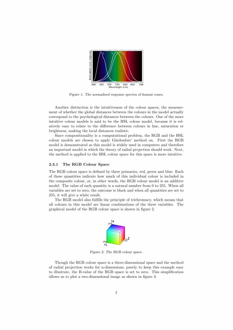
Figure 1: The normalized response spectra of human cones.

Another distinction is the intuitiveness of the colour spaces, the measure-ment of whether the global distances between the colours in the model actuallycorrespond to the psychological distances between the colours. One of the moreintuitive colour models is said to be the HSL colour model, because it is rel-atively easy to relate to the difference between colours in hue, saturation orbrightness, making the local distances realistic.

Since compositionality is a computational problem, the RGB and the HSLcolour models are chosen to apply Gardenfors’ method on. First the RGBmodel is demonstrated as this model is widely used in computers and thereforean important model in which the theory of radial projection should work. Next,the method is applied to the HSL colour space for this space is more intuitive.

2.3.1 The RGB Colour Space

The RGB colour space is defined by three primaries, red, green and blue. Eachof these quantities indicate how much of this individual colour is included inthe composite colour, or, in other words, the RGB colour model is an additivemodel. The value of each quantity is a natural number from 0 to 255. When allvariables are set to zero, the outcome is black and when all quantities are set to255, it will give a white result.

The RGB model also fulfills the principle of trichromacy, which means thatall colours in this model are linear combinations of the three variables. Thegraphical model of the RGB colour space is shown in figure 2.

Figure 2: The RGB colour space.

Though the RGB colour space is a three-dimensional space and the methodof radial projection works for n-dimensions, purely to keep this example easyto illustrate, the B-value of the RGB space is set to zero. This simplificationallows us to plot a two-dimensional image as shown in figure 3.

7

When we apply radial projection, we need two convex sets. In this case oneconvex set is the entire space shown in figure 3, the second set is illustrated bythe black square. The next step is to take an arbitrary origo in the intersectionof the two convex sets, which we call 0. Then, we select a point that we think isa typical green, for example, point x. To map this typical greenish colour to theintersection, we draw a straight line between the origo and this typical colour.This line crosses two boundaries, the one with the subset, where the crossing iscalled y0 and the intersection with the outer bound, called x0.

Consequentially, radial projection shows a correspondence between the dis-tance from the origo to the inner boundary and the distance from the origo tothe outer boundary, which gives the following formula:

d(O, y0)

d(O, y)=d(O, x0)

d(O, x)(1)

leading us to point y.

In other words; when two convex sets have a common point, we map oneconvex set to another by scaling them linearly to fit one another. So when wehave a point outside the intersection (x ) and we map it to the inside of theintersection, we get the representative inner point (y) to replace the outlier x.

For this particular example, it would mean that the green colour, referred toby point x, with RGB-values [20, 230, 0], would be represented by point y. Thisnew colour has the following RGB-values: [100, 160, 0]. When we look at thiscolours side by side, they are not the same shade, but they are definitely bothrepresenting a green colour. If we were to choose a typical green colour fromthe inner convex set, it would even be sensible to choose the y-colour.

Figure 3: The RGB colour space, where B = 0, the origo is in the middle of thesubspace, x represents a typical green colour and z a typical yellow colour. On theright of the plot, the first line shows the colours represented by x and y, respectivelyand the bottom two squares show the two colours represented by z and w, respectively.

However, there are a couple of sidenotes to address. First of all, the bluecolour is missing in this example, by setting the B to zero. This might have led

8

to a different result; maybe the green colour represented by x would not be atypical green colour if we could add some blue.

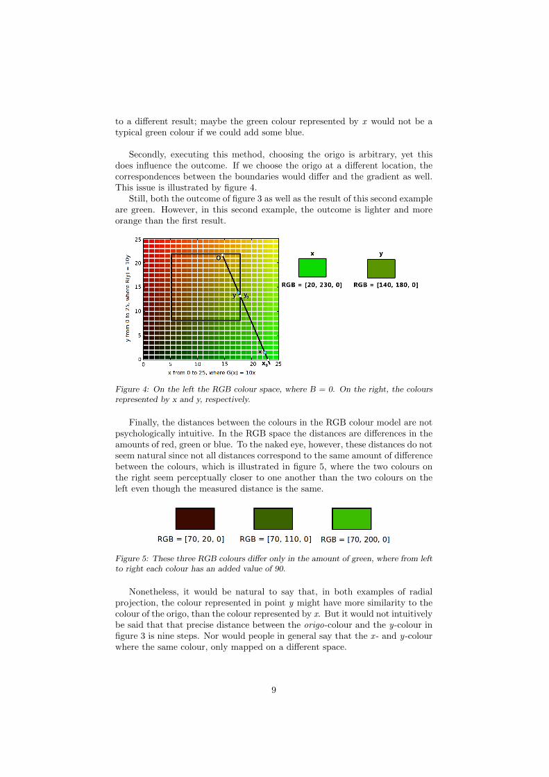
Secondly, executing this method, choosing the origo is arbitrary, yet thisdoes influence the outcome. If we choose the origo at a different location, thecorrespondences between the boundaries would differ and the gradient as well.This issue is illustrated by figure 4.

Still, both the outcome of figure 3 as well as the result of this second exampleare green. However, in this second example, the outcome is lighter and moreorange than the first result.

Figure 4: On the left the RGB colour space, where B = 0. On the right, the coloursrepresented by x and y, respectively.

Finally, the distances between the colours in the RGB colour model are notpsychologically intuitive. In the RGB space the distances are differences in theamounts of red, green or blue. To the naked eye, however, these distances do notseem natural since not all distances correspond to the same amount of differencebetween the colours, which is illustrated in figure 5, where the two colours onthe right seem perceptually closer to one another than the two colours on theleft even though the measured distance is the same.

Figure 5: These three RGB colours differ only in the amount of green, where from leftto right each colour has an added value of 90.

Nonetheless, it would be natural to say that, in both examples of radialprojection, the colour represented in point y might have more similarity to thecolour of the origo, than the colour represented by x. But it would not intuitivelybe said that that precise distance between the origo-colour and the y-colour infigure 3 is nine steps. Nor would people in general say that the x - and y-colourwhere the same colour, only mapped on a different space.

9

2.3.2 The HSL Colour Space

The abbreviation of HSL stands for hue, saturation and lumination. The hueis the value to which the colour seems similar to one, or to proportions of twoother colours [3]. In other words, the hue of the colour yellow would be closerto the hue of orange than to the hue of blue since yellow and orange look moresimilar than yellow and blue. The saturation is the degree to which the huediffers from a neutral gray, running from 0% to 100%. If the saturation is lower,the colour will be closer to gray. Lastly, the lumination indicates the brightnessof the colour, where at 0% the colour is completely black, 50% gives a purecolour and turns white at 100%.

The HSL colour space is also referred to as the colour spindle, where the ra-dius is defined by the value of saturation. The height depends on the brightnessof the colour and the rotation around the spindle depends on the hue. This isshown in figure 6.

Figure 6: The graphical representation of the HSL colour model.

To easily illustrate this example, the value of the lumination is set to a half.Again two convex sets are needed, this time two circles. Then, when we take thecentre of the inner circle as origo and a colour in the colour space, the resultingcolour will always be a less saturated version of the same colour, because everyline from the centre of both circles will always make a radius, which representsthe saturation of the HSL colour space (figure 7). Furthermore, when a lesssaturated yellow than the displayed yellow in figure 7 would be chosen as startingpoint, the result would be even less saturated than the outcome shown in thepicture.

So looking from the origo of the circle, this method seems intuitive; whenwe select a bright yellow and map this to grayisch colours, we end up with agrayish yellow. Also, when we were to choose a less bright yellow, we wouldfinish with an even grayer form of yellow.

Nonetheless, despite of this intuitiveness, this colour model too, faces theproblem of the origo. Since the origo is not a specified point, not all outcomesare logical. This problem is illustrated by figure 8, where the origo is not in thecentre of both circles, which directly leads to a very different result.

Concisely, in the case of two circles of which one is placed exactly in demiddle of the other circle and where the origo is chosen in the middle of both

10

Figure 7: On the left the HSL colour space, where L = 0.5, x represents a typicalyellow colour and z represents a typical green colour. On the right, on top the coloursrepresented by x and y, respectively and below the two colours represented by z andw, respectively.

circles, the radius will give the same colour with less saturation, every other linewill directly change the slope and move the representative inlier to a differentcolour, since the colours, which we believe are different from each other, arearranged by hue.

Furthermore, the other two objections mentioned in the previous section alsowithstand this colour model. This model too, is incomplete by fixing the lumi-nation and lastly, although this model is more intuitive than the RGB colourspace, these distances remain psychologically unintuitive. Even though it is in-tuitive to distinguish between colours based on hue, saturation or brightness,making the local distances natural, globally, the distances are still unintuitive.This problem is illustrated by figure 9, in which all colours differ the sameamount in hue. However, the two colours on the right seem more similar thanthe two colours on the left even though the measured distance is equal to oneanother.

Also, in the HSL colour model, it would be natural to have a special distancemetric since the difference in hue has more impact on the changes between thecolours than the saturation. In figure 10 the first and the second colour differ twosteps in hue and the second and last colour differ two steps in saturation. In thispicture it is clearly shown that the first and second colour have a perceptuallygreater difference than the second and the third.

2.4 Points of Discussion

For both colour models the same three problems seem to arise; the fixing of onevalue, the psychologically unintuitive distances and the choosing of the origo.

First of all, both colour models are incomplete since in both cases one of the

11

Figure 8: On the left the HSL colour space, where L = 0.5. On the right, the coloursrepresented by x and y, respectively.

Figure 9: Four colours from the HSL space, from left to right all 36 degrees apart inhue.

three values has been fixed. However, the method should provide a solid theoryfor all combinations of two (partially) overlapping convex sets, so this shouldalso be true for two convex sets that happen to lay in a two-dimensional planeof the colour space.

The next point of critique is the unintuitiveness of the colour models, whichis a well-known problem for psychologists. This has led to more intuitive modelslike the Munsell colour space, where distances between colours correspond toreal perception thresholds. Perhaps the theory would provide better results fordifferent colour spaces. Nevertheless, the RGB colour model is relevant as theproblem of compositionality is important in computer sciences. The RGB colourspace is widely used in computers and therefore an important model in whichthe theory of radial projection should work.

Also, even though Gardenfors’ method is only tested on colour spaces, thetheory should work for all conceptual spaces. However, the fact that colourspaces are not perfectly suitable for this theory, does not mean that the theoryin general is faulty for every other conceptual space.

Finally, it might not even be possible to find a globally realistic solution us-ing the Euclidian metric and maybe a different metric, like Riemannian metric,would provide more intuitive results.

Lastly, the most important point of improvement this theory needs is thechoosing of the origo and the prototypical colour. When radial projection is

12

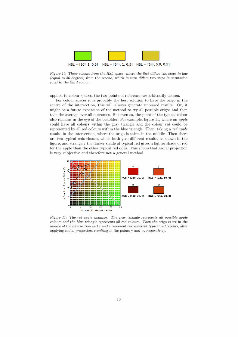
Figure 10: Three colours from the HSL space, where the first differs two steps in hue(equal to 36 degrees) from the second, which in turn differs two steps in saturation(0.2) to the third colour.

applied to colour spaces, the two points of reference are arbitrarily chosen.For colour spaces it is probably the best solution to have the origo in the

centre of the intersection, this will always generate unbiased results. Or, itmight be a future expansion of the method to try all possible origos and thentake the average over all outcomes. But even so, the point of the typical colouralso remains in the eye of the beholder. For example, figure 11, where an applecould have all colours within the gray triangle and the colour red could berepresented by all red colours within the blue triangle. Then, taking a red appleresults in the intersection, where the origo is taken in the middle. Then thereare two typical reds chosen, which both give different results, as shown in thefigure, and strangely the darker shade of typical red gives a lighter shade of redfor the apple than the other typical red does. This shows that radial projectionis very subjective and therefore not a general method.

Figure 11: The red apple example. The gray triangle represents all possible applecolours and the blue triangle represents all red colours. Then the origo is set in themiddle of the intersection and x and z represent two different typical red colours, afterapplying radial projection, resulting in the points y and w, respectively.

13

3 Composing with the Reduced Tensor Product

The theory of the reduced tensor product is based on the vector representationof concepts. Within this framework, concept similarity is a function of distance,where semantically related concepts are closer to one another than semanticallyless related words, which is also shown in figure 12 [11]. For example, theconcept mammal will be more similar to creature than lamp.

Figure 12: An example of semantic space, where similar concepts are closer than lesssimilar concepts.

On a more detailed level, every concept is represented by its own vectorof which every component represents the degree to which that component isrepresentative to the concept, which is also called the cue validity [2]. Moreexplicitely, the vector contains as many components as there are concepts inthe represented world and the more similar the component is to the concept,the higher the value of that specific component. This vector is based on theprototype theory, where an object instances a concept only to the extent thatit is similar to the prototype of the concept [13].

For instance, if our world contains the concepts red, blue and green, the con-cept green would be a vector with three components, namely the three colours,where the most similar colour would have the highest value. So the vector ofthe concept green, could have a vector like: [0.3, 0.7, 1], where red is 0.3, andblue 0.7 representative to the concept green.

This factor of representiveness of every component is based on the distancebetween the component and the most prototypical instance of the concept. So,within a semantic space, mathematically speaking, a distribution is created,where the peak of the curve lies on top of the most prototypical concept andthe curve fans out in every direction.

Next, these vectors can be used to calculate combinations of concepts. Whentwo concepts are combined, the reduced tensor product is applied, resulting ina third vector, having the highest value for the most prototypical instance forthe combination of the two concepts.

Originally, the tensor product representation was used by Smolensky forthe connectionist representation of variable bindings [20]. However, the ten-sor product provided a growing dimensionality, as when a n-dimensional vectorand a m-dimensional vector are combined through this direct outer product,the result is a nm-dimensional vector. To avoid this problem, Plate proposedto use holographic reduced representations, which uses circular convolution toassociate items [16]. Unfortunately, this mathematical operation is, unlike ourapplication in linguistics - a semantic space -, translation invariant. Severalresearchers have also proposed simple multiplication operations (cf. [2],[11]),

14

which is related to earlier proposals by Zadeh and Hajek in fuzzy logic wherethe relevant operation is called the product t-norm ([7], [25]).

The next section will describe the properties that are needed to use thereduced tensor product. Next, the method will be explained with the propermathematical background. Also an elaboration on the term reduced tensor prod-uct will be given in this part.

3.1 Assumptions

There are a couple of properties this method requires:

• Semantic space. This method is applied to a semantic space, where se-mantically related concepts are more nearby than less related concepts.

• (Proto)typicality. The method is based on the prototype theory, whichassigns a degree of typicality for every instance to a concept based on thesimilarity between the instance and the prototype.

• Euclidean space. All calculations take place in the Euclidian space.

3.2 Method

This account of semantics provides a framework for representing the meaning ofword combinations in vector space, where points that are close together in thisspace are semantically similar and points that are far apart are semanticallydistant [12][23].

Mathematically, the typicality of instance i within concept A, written asci(A), can be calculated using the following distance function:

ci(A) = ne−1T d(PA,i)k (2)

where the distance function d gives the Euclidean distance between the instancei and the prototype PA of concept A. The prototype PA also is one of the in-stances of A, resulting in the peak of the distribution. The terms T and k areused to scale the distribution, towards a clearer peak in the resulting curve;these two variables will be explained in depth in the next section. This cal-culation of the cue validity is used for every instance, resulting in a vector ormatrix, depending on the meaning space. Finally, the entire concept is normal-ized, which is indicated by the term n.

When this formula is applied to two concepts, the resulting plot containstwo peaks, which represent the two prototypes and both concepts have theirown density distribution (figure 13). The x-axis represents the instances inthe world, ordered semantically. The y-axis gives the degree of typicallity theinstance holds.

Next, to combine two concepts, the two distributions are merged to a newdistribution. In other words, the reduced tensor product is applied as means ofbinding one distribution to another to produce structured representations [12]:

(A⊗B)i = AiBi (3)

15

Figure 13: An example of vector space, where concept A has its prototype at (2),shown in blue, and the other concept, B at (12), shown in green. Also, the variablesare set: T = 2 and k = 1.5.

However, the dimension of the tensor product is the product of the dimen-sions of the original spaces, so, in the case of the two vectors the resultingproduct gives a matrix. Because a growing dimensionality is not welcome, areduced tensor product is taken. This means we do not use the entire resultingmatrix, but only the diagonal of this matrix. This has the advantage that thedimensionality will stay equal. Then, this new vector will be normalized as well.This resulting vector also shows a peak, which represents the prototypical com-bination of the two previous prototypes, which we will call the target. When thetwo distributions shown in figure 13 are combined through this reduced tensorproduct, the following distribution arises (figure 14).

Figure 14: An example of vector space, where concept A has its prototype at (2)(blue) and the other concept, B, at (12) (green). Also, the variables are set: T = 2and k = 1.5. The reduced tensor product then gives a third distribution, shown inred, which gives a prototypical combination, t, at (7).

3.3 Mathematical Background

3.3.1 Three Aligning Peaks

A very important property of this method is that the three peaks of the disti-butions are aligned (figure 15).

Figure 15: The vector space, where concept A has its prototype at (3,5) and the otherconcept at (10,15), T = 2 and k = 1.5. The reduced tensor product then gives a thirddistribution, of which the maximum is aligned with the two prototypes and indicatedby the letter t.

16

When a line is drawn between the two prototypes and we were to look forthe local maximum on this line, the point would have to lie in between the twoprototypes, since the highest correspondence of both distributions lies therebased on Euclidean distances. Next, if we were to deviate from this line, thedistance to the prototypes will only grow bigger due to the triangle inequality,making the cue validity smaller and smaller. Therewith concluding that the localmaximum on the line actually is the global maximum, because every movementoff the line will only shrink the value of the cue validity.

Nevertheless, this feature does rely on a couple of properties of the distribu-tions. The first property is the Euclidean geometry, where the shortest distancebetween two points is a straight line. Secondly, both distributions have to besymmetrical and monotonically decreasing. Fulfilling these properties cause thecombined distribution to be on a straight line between the two prototypes ofthe concepts.

3.3.2 The Variables Explained

In the formula for calculating the distributions, two variables occur, namely Tand k. The T -variable is a scalar, when the value increases the distribution willspread out more (figure 16).

In other words, the variable T defines the decay of the distribution. In effect,the higher the value of variable T , the lower the peak of the distribution. Sowhen the value of T differs between concept A and B, the distributions willdiffer in height and decay, and the target will move towards the distributionwith the higest decay (figure 17). However, it should be noted that T needs tohave a positive value to conserve the properties of the distribution function.

The second variable used is the variable k, which is needed to make a dis-tribution with a peak, which is necessary to point out the combined prototype.When k is set to one, the third distribution will be a constant instead of adistribution with a peak. Mathematically, the following formula is used whenk = 1:

(A⊗B)i,i = nA ∗ nB ∗ e−d(PA,i) ∗ e−d(PB ,i) (4)

where there are two concepts, A and B, which both have their own prototypes,PA and PB , respectively. Then, for every instance i the product of the normal-ization factors and the exponential distance functions are taken.

This function can be rewritten as:

(A⊗B)i,i = nA ∗ nB ∗ e−d(PA,i)−d(PB ,i) (5)

However, since the distance between the two prototypes PA and PB is constant,the movement of i will only move the ratio between the two prototypes, but willnot affect the outcome:

−d(PA, i) − d(PB , i) = −(i− PA) − (PB − i) = PA − PB (6)

This problem can be solved by adding a power to which the distances aretaken. This causes a difference between the distance from i to PA and thedistance from i to PB , which makes for a distribution with a peak (figure 18).Also, if k differs between the two distributions, the target will move towards

17

(a) T = 0.5 (b) T = 1

(c) T = 2(d) T = 5

Figure 16: Examples of the vector space, where one concept has its prototype at (2)and the other concept at (8), k = 1.5 and T variates. The reduced tensor productthen gives a third distribution, shown in red, which gives a prototypical combinationat (5).

(a) TA = 2 and TB = 4. (b) TA = 2 and TB = 8.

Figure 17: Examples of the vector space, where concept A has its prototype at (2)(blue) and the other concept, B, at (12) (green). Also, the variables are set: k is equalfor both distributions and set to 1.5, the value of T differs. The reduced tensor productthen gives a third distribution, shown in red, which gives a prototypical combination,with its peak at t.

18

(a) k = 0.5

(b) k = 1

(c) k = 1.5

(d) k = 3

Figure 18: Examples of the vector space, where one concept has its prototype at (2)and the other concept at (8), T = 2 and k variates. The reduced tensor product thengives a third distribution, shown in red, which should give a prototypical combinationat (5).

the distribution with the highest value of k, since the placement of the targetdepends on the difference between the distributions and the distribution withthe highest power will have the highest outcome (figure 19). Furthermore, kshould have a positive value as well. When k is negative, the distribution isupside down, meaning the cue validity of the prototypes will become zero, in-stances with normally the highest values suddenly have the lowest values andvice versa, resulting in a valley instead of a peak.

Another property of the two variables is that if T and k are equal for bothdistributions, the peak of the combined prototype will always lie in the middleof the two peaks. This can be explained with the following equations, where tstands for target, the combined prototype:

t = maxi(nA ∗ nB ∗ e− 1T d(PA,i)k− 1

T d(PB ,i)k) (7)

As discussed in the previous section, the three peaks are aligned, so PA can beused as origin of the line, which entails that PA can be replaced by zero and thedistances can be rewritten as i and PB − i (figure 20).

t = maxi(nA ∗ nB ∗ e− 1T ik− 1

T (PB−i)k) (8)

To find the value of t, the derivative of this formula should be equal to zero.The instance i for which this formula is zero, will be the i with the maximumvalue, named target t:

δ

δt(nA ∗ nB ∗ e− 1

T tk− 1T (PB−t)k) = 0 (9)

19

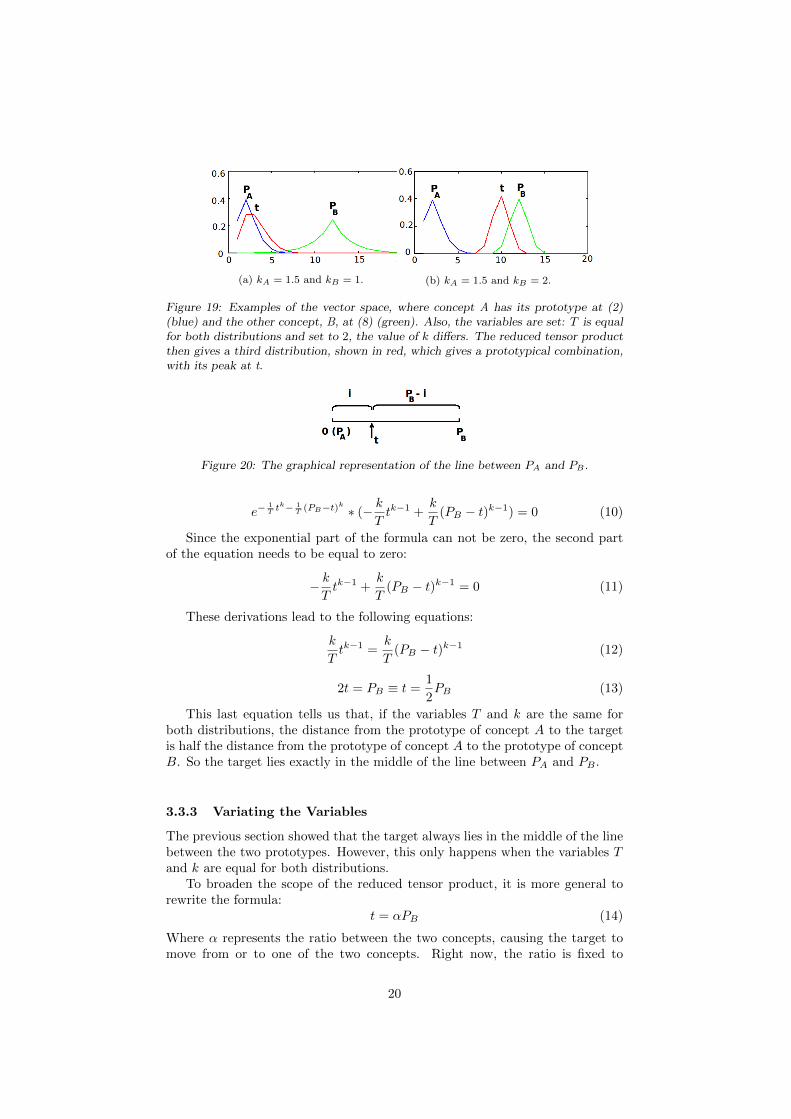
(a) kA = 1.5 and kB = 1. (b) kA = 1.5 and kB = 2.

Figure 19: Examples of the vector space, where concept A has its prototype at (2)(blue) and the other concept, B, at (8) (green). Also, the variables are set: T is equalfor both distributions and set to 2, the value of k differs. The reduced tensor productthen gives a third distribution, shown in red, which gives a prototypical combination,with its peak at t.

Figure 20: The graphical representation of the line between PA and PB .

e−1T tk− 1

T (PB−t)k ∗ (− k

Ttk−1 +

k

T(PB − t)k−1) = 0 (10)

Since the exponential part of the formula can not be zero, the second partof the equation needs to be equal to zero:

− k

Ttk−1 +

k

T(PB − t)k−1 = 0 (11)

These derivations lead to the following equations:

k

Ttk−1 =

k

T(PB − t)k−1 (12)

2t = PB ≡ t =1

2PB (13)

This last equation tells us that, if the variables T and k are the same forboth distributions, the distance from the prototype of concept A to the targetis half the distance from the prototype of concept A to the prototype of conceptB. So the target lies exactly in the middle of the line between PA and PB .

3.3.3 Variating the Variables

The previous section showed that the target always lies in the middle of the linebetween the two prototypes. However, this only happens when the variables Tand k are equal for both distributions.

To broaden the scope of the reduced tensor product, it is more general torewrite the formula:

t = αPB (14)

Where α represents the ratio between the two concepts, causing the target tomove from or to one of the two concepts. Right now, the ratio is fixed to

20

the middle of the line, causing α to be equal to a half. But if the variable Tdiffers between the two prototypes, the target would still align with the twoprototypes, but would also move towards the concept with the highest decay(the lowest value of T ). The derivation of α can be calculated starting with theformula for t, also defined by equation (8), but now the values of TA and TBare defined seperately:

t = maxi(nA ∗ nB ∗ e−1

TAik− 1

TB(PB−i)k

) (15)

Then, the derivative of the formula should be set to zero to find the maximumvalue for i, namely the target:

e− 1

TAtk− 1

TB(PB−t)k ∗ (− k

TAtk−1 +

k

TB(PB − t)k−1) = 0 (16)

Since the exponential expression at the beginning of the formula can not beequal to zero, the second part of the formula must be zero in order to solve theequation:

− k

TAtk−1 +

k

TB(PB − t)k−1 = 0 (17)

This simplification leads to the following equation:

1

TAtk−1 =

1

TB(PB − t)k−1 (18)

Next, the target can be isolated in the formula:

t =PB

1 + (TB

TA)

1k−1

(19)

This equation gives us the formula for α, depending on the values of TA, TBand k:

α =1

1 + (TB

TA)

1k−1

(20)

So if the value of T differs between the two distributions, the reduced tensorproduct still provides a linear function. Furthermore, if the value of TA were togrow and the value of TB would remain the same, the value of the denominatorof α would have its limit at one and the target will end up at PB . Because: thehigher the value of TA, the lower the decay of distribution A and the target willmove towards the prototype of concept B. In short, the value of α depends onthe ratio between TA and TB and when TA grows to infinity or when TB shrinkstowards zero, the limit of α is one and when TA shrinks towards zero or whenTB grows to infinity, the limit of α is zero. This means α will always have avalue between zero and one, where zero represents the point of the prototype ofconcept A and one is equal to the position of the prototype of concept B. Orin other words, when T differs between the two distributions, the decay of thedistributions differs, causing the target to move towards the distribution withthe highest decay - i.e. the lowest value of T .

21

Another possibility is to differ the value of k instead of T . To make it easierto read, the k of the distribution of concept A will be called k and the power ofconcept B will be called m:

t = maxi(nA ∗ nB ∗ e− 1T ik− 1

T (PB−i)m) (21)

Then, to find the maximum value of t, its derivative has to be equal to zero:

e−1T tk− 1

T (PB−t)m ∗ (− k

Ttk−1 +

m

T(PB − t)m−1) = 0 (22)

Similar to the previous calculations, only the second part needs to be equal tozero:

− k

Ttk−1 +

m

T(PB − t)m−1 = 0 (23)

However, unlike the previous calculations for a differing T , the equations fordiffering the value of k lead to a complicated formula:

(k

m)

1m−1 t

k−1m−1 + t = PB (24)

Unfortunately this equation can not be solved in a general matter. So, insummation, differing T between the two distribution gives a linear functionthat can be compared to the method of radial projection. However, differingthe value of k between the two methods leads to an unsolvable formula and istherefore unwanted for the comparison of the two methods.

3.4 Points of Discussion

A couple sidenotes should be addressed using this method. Generally, there aretwo main problems: the initialization and the intuitiveness of the method.

Before the method can be executed, the variables have to be set and theprototypes need to be chosen, which can be very subjective. This is also shownin the colour models discussed in de previous chapter. So in order to make thismethod work, a consensus should be made regarding the prototypes and thevariables as well, since they define the slope of the distribution.

Next, the intuitiveness could be improved. Modeling concepts to a intuitivespace is a very difficult issue to solve. Even though it seems intuitive that seman-tically related concepts are more nearby than semantically unrelated concept,the precise distances between the concepts remain an obstacle.

Also, using this method, the distributions have two properties that mightnot intuitively be accurate. The first property is that the distributions fanout through the entire space, meaning that there are no boundaries betweenconcepts. So even if two concepts are totally unrelated, if they both lie withinthe same conceptual space, they will still have a measure of typicallity. Forexample, in figure 21 the distribution of the concept orange would still providea chance for the orange colour itself of being a green colour.

Finally, these distributions fan out equally in every direction. Figure 21shows the flaw of this assumption; not all equal distances have the same equal

22

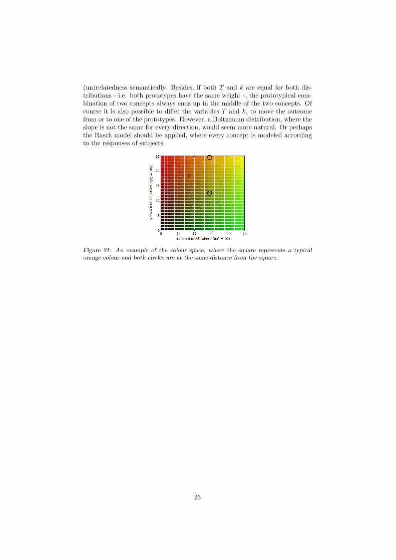
(un)relatedness semantically. Besides, if both T and k are equal for both dis-tributions - i.e. both prototypes have the same weight -, the prototypical com-bination of two concepts always ends up in the middle of the two concepts. Ofcourse it is also possible to differ the variables T and k, to move the outcomefrom or to one of the prototypes. However, a Boltzmann distribution, where theslope is not the same for every direction, would seem more natural. Or perhapsthe Rasch model should be applied, where every concept is modeled accordingto the responses of subjects.

Figure 21: An example of the colour space, where the square represents a typicalorange colour and both circles are at the same distance from the square.

23

4 Results and Discussion

4.1 Conceptual Comparison

Although the method of radial projection and the method of the reduced tensorproduct seem to be very different, there actually are just a few dissimilarities.The major difference between the two methods is that Gardenfors’ method isbased on a meaning space in which concepts are convex sets and have bound-aries. Whereas the method of the reduced tensor product uses distributionfunctions to formulate concepts throughout an entire semantic space. However,it should be noticed that this causes a similar constraint on both methods; toachieve radial projection, all concepts must be modeled using convex sets, butthe reduced tensor product also knows a convexity assumption. When there areseveral prototypes in the same semantical space and we were to look at everyinstance seperately to see to which prototype they belong - i.e. to look for whichprototype they have the highest cue validity -, and then assign the instances toone prototype, a Voronoi tessellation occurs. Since every cell of a Voronoi di-agram is a convex set by definition, the reduced tensor product creates convexconcepts as well [24].

The biggest semantic difference between the two methods is the notion ofconcepts having or not having boundaries. When we take the RGB colour spaceas an entire meaning space it seems logical to give the colour-concepts bound-aries, because the concept red should not intervene with the concept gray. How-ever, it is not possible to make a neutral gray colour without using some redand secondly, both concepts indicate a colour so they should be connected onsome semantic level. On the other hand, looking at a colour model, the se-mantic definition that all instances within this model are indeed colours, wasalready established by choosing this meaning space. So perhaps the biggest se-mantic boundary was already chosen. Nevertheless, perhaps concepts indicatedwithin colour spaces should have boundaries, whereas concepts within differentmeaning spaces should not have boundaries, or vice versa.

This notion actually leads to a psychological issue, whether concepts haveboundaries and whether semantic models can be intuitive. Radial projectionrequires two points, an origo and a typical instance in one of the two concepts,both chosen subjectively. The second method also requires two subjectivelychosen points, the two prototypes. Even if all people were to choose the samepoints for each method, the question of intuitiveness would still remain. Thisproblem remains, because semantic models translate the difference in meaninginto distances. The distances between meanings are not psychologically intu-itive and perhaps Euclidean metric should only be used as a first approximation.

However, apart from these differences between the methods - the convexregions versus the distance distributions and concepts modeled with our with-out boundaries - the Euclidean distances along a linearly ordered line are usedin both methods. Where the reduced tensor product uses distributions thatresult in a composed concept on the line between the two prototypes, radialprojection draws a line between an arbitrary origo, through a prototype, to theouter boundary. Next, Gardenfors’ method uses the correspondence betweenthe length of the line from the origo to the outlying prototype and outer bound-

24

ary and the length of the line from the origo to the inlying composed conceptand the inner boundary. So basically, the placement of the composed concepton the line between two prototypes is either defined by the ratio of the bound-aries of the concepts or by the ratio in weight of the prototypes of the concepts.The next section will cover the mathematical correspondence between the twoproportions.

4.2 Mathematical Comparison

To compare the two methods, they both need to be reduced to a comparableform. Fortunately, both methods can be easily reduced to a straight line. In themethod of radial projection, this line goes from the origo to the outer boundaryof the entire space, crossing the target concept, the inner boundary and thetypical outlying concept. Using the reduced tensor product, this line starts atthe prototype of one concept and ends in the prototype of the second concept.

Because of the steady ratio between the two concepts and the combinedconcept caused by the reduced tensor product, this section will first recall theformula for this method. Next, this formula will be compared to the mathemat-ical foundation of radial projection.

To compare the two methods, both lines need to be aligned. Firstly, thereduced tensor product can be described by a linear function, as explained insection 3.3.3, with the following formula:

t = αPB (25)

However, it is important to repeat that this formula only has a differing Tfor both distributions, but that the k is equal, because we need a linear functionto compare the two methods. Next, to align the method of radial projectionwith the proposed line of the reduced tensor product, it seems natural to replacethe origo of radial projection with the prototype of concept A and the typicalsecond concept, x, with the prototype of concept B (figure 22 and figure 23).

Figure 22: The RGB colour space, where blue = 0, the origo (PA) is in the middleof the subspace and x (PB) represents a typical yellow colour. Above the line are theterms that are replaced by the terms below the line.

Radial projection makes use of the following equation:

d(O, y0)

d(O, y)=d(O, x0)

d(O, x)(26)

25

Figure 23: Representation of the line.

When the methods are aligned, and if the line of both methods begin in thesame point, namely PA, every distance from PA to an arbitrary point on theline can be replaced by simply the placement of the arbitrary point on the lineitself:

y0t

=x0PB

(27)

This leads to the following equation, ending in a simple formula for t :

t =PBy0x0

(28)

Now formula (28) can be compared to the equation for t in for the reducedtensor product, given in equation (25):

PBy0x0

= αPB (29)

Resulting in the following equation:

y0x0

= α (30)

This last formula shows the correspondence between the ratio of the innerand outer boundary and the ratio of the two concepts. So if the target lies inthe middle of the two concepts - i.e. when α is equal to a half -, the innerboundary must be half the distance to the prototype of concept A comparedto the distance from the outer boundary to the prototype of concept A. Withthis equation the results of the reduced tensor product can be used to calculatethe boundaries for radial projection. Or, in short, the ratio between the innerand outer boundary in radial projection is equal to the ratio between the twoprototypes of the concepts, depending on the values of TA, TB and k.

4.3 Discussion

The results regarding the comparison of the two methods bring the conclusionthat, if attributive modification is calculated using Euclidean metric, the meth-ods actually are interchangeable. In other words, starting with the reducedtensor product, the parameters of Gardenfors’ model can be reconstructed tofind the same combined prototype and starting with radial projection it is possi-ble to reconstruct the ratio in weights between the two prototypes of the reducedtensor product model. However, this is only possible under the assumption thatthe origo and typical instance of the model for radial projection are chosen atthe same locations as the two prototypes from the reduced tensor product.

Then, the only remaining obstacles are the choosing of the prototypes or theorigo and typical instance, the potential boundaries of the concepts and the in-tuitiveness of the semantic model itself. The choosing of all these points depend

26

on the individual and would require psychological research to achieve a commonanswer. Furthermore, if the prototypes were chosen based on popular opinions,a normal distribution with a mean and a deviation seems natural. However,people might still need boundaries for every concept instead of a distributioncovering the entire meaning space.

Concisely, two domains can be further explored. The first is the modelingof a semantic space. It is possible that colour spaces are a bad example forattributive modification, or perhaps different colour spaces than the ones usedin this thesis should be used, like the more intuitive model of Munsell. Whenattributive modification is tested on semantic models, the model should containintuitive distances between its instances. To achieve this goal, the notion ofusing a different metric than the Euclidean metric system should be exploredas well. However, when people do decide to use colour models for attributivemodification, psychological research must be done to find more similarities be-tween people in finding two prototypes and their combined colour. Also, if theprototypes are chosen based on votes, a distribution seems natural. However,if boundaries turn out to be a very natural mold as well, perhaps it is advanta-geous to combine the two methods.

The second domain that needs exploring is the mathematical point of view,which metric system should be used or which distribution functions would ren-der the best results. Whether concepts do or do not have boundaries, bothmethods make use of convex sets and linearly ordered instances. Perhaps thetwo could be combined to distributions within convex regions with boundaries.Or perhaps a different distribution function, not being symmetrical or mono-tonically decreasing, would generate more intuitive results.

27

5 Conclusion

To understand language, pasting the meanings of seperate words together is notenough. When words are merged into a sentence, or even a part of a sentence,their meanings are merged as well. Focussing on the combination of a modifierand a head, multiple methods have been developed to solve attributive mod-ification. Though there are two kinds of attribution modification; direct andindirect modification, most methods focus on the latter.

One of the most recent methods is the method of Gardenfors. This methodis based on the property that Gardenfors ascribes to inner concepts of men-tal spaces: convexity. Based on this mathematical property, homeomorphismbetween two concepts can always be achieved through radial projection.

Making use of three assumptions - the existence of mental spaces, the con-vexity and Euclidean space -, two convex concepts with an overlapping part canbe mapped into the intersection with a one-to-one correspondence. When twoconcepts overlap, an arbitrary origo is taken in the intersection and a typicalinstance is taken in one of the two concepts. Next, the distance from the origoto the typical instance with respect to the outer boundary of the correspond-ing concept is taken as a ratio for the distance from the origo to the resultingcombination with respect to the boundary of the intersection.

To test this method, radial projection was applied to colour spaces, becausethese are the only modeled meaning spaces. Unfortunately, for both the RGBand the HSL colour space the method did not seem to render intuitive results.This problem could be due to the colour models, because in both cases one valueof the model was fixed. Even though this should not cause a problem, perhapsusing the entire colour spaces would provide different results. The second prob-lem caused by the colour models is the unintuitiveness of the distances betweencolours, which might be solved by using different colour models or a differentmetric system. However, the perception of colours remains very subjective andtherefore might not be suitable as an example for meaning spaces. Perhapscolour adjectives should even have its own behavioural class.

Finally, the most relevant problem this method encountered is the place-ment of the origo. Although the one-to-one correspondence between two setswith an overlap is possible for every arbitrary placement of the origo within theintersection, it does influence the placement and slope of the line from the origoto the typical instance. Furthermore, this typical instance is also subjective. Inshort, since both the origo and the typical instance are subjective, the resultdiffers per person, making the method subjective instead of general.

The second method is based on the prototype theory and represented by avector space. The prototype theory originates from the cognitive sciences andstates that every concept has one member that is more characteristic than theothers. When a concept is represented by a vector, this vector contains a degreeof typicality for every instance of the concept. So if this representation is used ina semantic space, all instances will be ordered based on their meanings and thedegree of typicality, called the cue validity, is defined as a function based on thedistance between the instance and the prototype of the concept. Then, plottingthe vectors, this will give a distribution with a peak on top of the prototype ofthe concept.

28

The next step is to find the prototypical combination of the two concepts,which is achieved by combining the two vectors that represent the concept ofthe head and the concept of the modifier. This method states that this shouldbe done by taking the reduced tensor product between the two vectors. To stopthe growing dimensionality of a regular tensor product, only the diagonal of thisproduct is taken, hence the name reduced tensor product. The resulting vectoralso shows a peak, representing the prototypical combination of the two originalconcepts.

Nevertheless, this method depends on two variables; the cue validity is notonly based on the distance between the prototype of the concept and everyinstance of the semantic space, but also influenced by the two parameters Tand k. Whereas T represents the decay of the distribution, causing a higher orlower peak, the variable k represents power to which of the distance betweenthe prototype and the instance is taken, which causes a bigger difference inmagnitude of the cue validity.

The most important feature of this method, based on the symmetrical andmonotonically decreasing distributions, is that the resulting peak aligns withthe two original prototypes. Furthermore, when the parameters T and k areequal for both distributions, the combined vector has its peak exactly in themiddle of this line between the prototypes.

However, this method also depends on subjectivity. First of all, the proto-types and the variables need to be set, which can differ between individuals.Next, the distance between semantically related and unrelated concepts formsan obstacle. Because the distributions are symmetrical and monotonically de-creasing, an equal distance from the prototype means to have an equal semanticdifference from the prototype, which is not an universal property of meaningspaces, as shown in the colour spaces. Also, however likely it seems that seman-tically similar meanings are closeby, exact distances are subjective as well. Andfinally, every instance in the semantic space will have a chance of having thesame meaning as the prototype, because the distributions fan out through theentire space, without any boundaries.

Since both methods use Euclidean metric and are based on linearly orderedinstances, they can be aligned mathematically. When the two points of radialprojection, the origo and the typical instance, are chosen at the same locationas the two prototypes of the reduced tensor product, a correspondence can befound between the two methods. This correspondence entails that the ratiobetween the inner and outer boundary of radial projection is equal to the ratiobetween the weights of the two prototypes. So if both prototypes have the sameweight, the target lies in the middle of the two prototypes and for Gardenfors’method the outer boundary of the concepts should be twice as far from the origoas the inner boundary.

Using this correspondence, only one difference between the methods remains:the modeling of concepts. The difference is the existence of boundaries; whereasthe reduced tensor product uses the entire meaning space for every concept,radial projection chooses a convex region within the semantic space for everyconcept. The notion of each concept having boundaries or being related toevery other concept is a psychological question and maybe even depends on theindividual. Perhaps some concepts should have boundaries while others shouldnot. Also, when a meaning space is already specialized to one aspect, like the

29

colour models, the biggest semantical boundary is already set.In short, when the mental space is convex and ordered semantically, and

two prototypical points are chosen, using Euclidean metric, both methods canbe used and by adjusting the ratio between the boundaries of radial projectionor the variables T and k of the reduced tensor product, the same result can befound. The only remaining difference would be the existence of boundaries ofthe concepts, which would depend on the psychological modeling of the conceptsand thus would be in the eye of the beholder.

30

References

[1] C. Berge. Topological Spaces. Mineola: Dover, 1997.

[2] R. Blutner. Concepts and bounded rationality: An application of niesteggesapproach to conditional quantum probabilities. Foundations of probabilityand physics, 5:302–310, 2009.

[3] D. Bourgin. The color space faq, 2004.

[4] J.R. Busemeyer and P.D. Bruza. Quantum Models of Cognition and Deci-sion. Cambridge University Press, 2012.

[5] C.P. Dolan and P. Smolensky. Tensor product production system: a modu-lar architecture and representation. Connection Science, 1(1):53–68, 1989.

[6] P. Gardenfors. Concept combination: a geometrical model. Lund University,1998.

[7] P. Hajek. Metamathematics of fuzzy logic. Kluwer, Dordrecht, 1998.

[8] G. Hoffmann. Cie color space, 2002.

[9] Gerhard Jger. The evolution of convex categories. Linguistics and Philos-ophy, 30:551–564, 2007.

[10] E. Landa and M. Fairchild. Charting color from the eye of the beholder acentury ago, artist albert henry munsell quantified colors based on how theyappear to people; specializations of his system are still in wide scientific use.American scientist, pages 436–443, 2005.

[11] J. Mitchell and M. Lapata. Vector-based models of semantic composition.In In Proceedings in ACL-08: HLT, 2008.

[12] J. Mitchell and M. Lapata. Composition in distributional models of seman-tics. Cognitive Science, 34(8):1388–1429, 2010.

[13] D.N. Osherson and E.E. Smith. On the adequacy of prototype theory as atheory of concepts. Cognition, 9(1):35–58, 1981.

[14] B.H. Partee. Privative Adjectives: Subsective plus Coercion. EmeraldGroup Publishing Limited, 2010.

[15] D. Pascale. A review of rgb color spaces. The BabelColor Company, Mon-treal, Tech. Rep, 2003.

[16] T.A. Plate. Holographic reduced representations: convolution algebra forcompositional distributed representations. 12th International Joint Con-ference on Artificial Intelligence, pages 30–35, 1991.

[17] T.A. Plate. A common framework for distributed representation schemesfor compositional structure. Connectionist systems for knowledge represen-tation and deduction, pages 15–34, 1997.

[18] T.A. Plate. Structured operations with distributed vector representations.Advances in Analogy Research: Integration of Theory and Data from theCognitive, Computational, and Neural Sciences, 1998.

31

[19] P. Smolensky. Connectionism, constituency and the language of thought.1988.

[20] P. Smolensky. Tensor product variable binding and the representation ofsymbolic structures in connectionist systems. Artificial Intelligence, 46(1–2):159–216, 1990.

[21] S. Susstrunk, R. Buckley, and S. Swen. Standard rgb color spaces. In Proc.IS&T/SIDs 7th Color Imaging Conference, pages 127–134, 1999.

[22] I. Tastl and G. Raidl. Transforming an analytically defined color space tomatch psychophysically gained color distances. In Electronic Imaging 1998Conference, 1998.

[23] P. Turney and P. Pantel. From frequency to meaning: Vector space modelsof semantics. Articial Intelligence Research, 37:141–188, 2010.

[24] M. Warglien and P. Gardenfors. Semantics, conceptual spaces, and themeeting of minds. Synthese, pages 1–29, 2007.

[25] L.A. Zadeh. A note on prototype theory and fuzzy sets. Cognition, 12:291–298, 1982.

32