Two Component Decomposition of Dual Polarimetric HH/VV SAR ...

remote sensing

Article

Two Component Decomposition of Dual PolarimetricHH/VV SAR Data: Case Study for the TundraEnvironment of the Mackenzie Delta Region, Canada

Tobias Ullmann 1,*, Andreas Schmitt 2 and Thomas Jagdhuber 3

1 Institute Geography and Geology, University of Wuerzburg, D-97074 Wuerzburg, Germany2 German Aerospace Center (DLR), German Remote Sensing Data Center, D-82234 Wessling, Germany;

[email protected] German Aerospace Center (DLR), Microwaves and Radar Institute, D-82234 Wessling, Germany;

[email protected]* Correspondence: [email protected]; Tel.: +49-931-31-86865

Academic Editors: Zhong Lu and Prasad S. ThenkabailReceived: 11 July 2016; Accepted: 8 December 2016; Published: 16 December 2016

Abstract: This study investigates a two component decomposition technique for HH/VV-polarizedPolSAR (Polarimetric Synthetic Aperture Radar) data. The approach is a straight forward adaption ofthe Yamaguchi decomposition and decomposes the data into two scattering contributions: surfaceand double bounce under the assumption of a negligible vegetation scattering component in Tundraenvironments. The dependencies between the features of this two and the classical three componentYamaguchi decomposition were investigated for Radarsat-2 (quad) and TerraSAR-X (HH/VV) datafor the Mackenzie Delta Region, Canada. In situ data on land cover were used to derive the scatteringcharacteristics and to analyze the correlation among the PolSAR features. The double bounceand surface scattering features of the two and three component scattering model (derived frompseudo-HH/VV- and quad-polarized data) showed similar scattering characteristics and positivelycorrelated-R2 values of 0.60 (double bounce) and 0.88 (surface scattering) were observed. The presenceof volume scattering led to differences between the features and these were minimized for landcover classes of low vegetation height that showed little volume scattering contribution. In terms ofseparability, the quad-polarized Radarsat-2 data offered the best separation of the examined tundraland cover types and will be best suited for the classification. This is anticipated as it representsthe largest feature space of all tested ones. However; the classes “wetland” and “bare ground”showed clear positions in the feature spaces of the C- and X-Band HH/VV-polarized data and anaccurate classification of these land cover types is promising. Among the possible dual-polarizationmodes of Radarsat-2 the HH/VV was found to be the favorable mode for the characterization of theaforementioned tundra land cover classes due to the coherent acquisition and the preserved co-pol.phase. Contrary, HH/HV-polarized and VV/VH-polarized data were found to be best suited for thecharacterization of mixed and shrub dominated tundra.

Keywords: Synthetic Aperture Radar (SAR); Polarimetric Synthetic Aperture Radar (PolSAR); dualpolarimetry; polarimetric decomposition; TerraSAR-X; Radarsat-2; tundra; arctic; Canada

1. Introduction

The decomposition of Polarimetric Synthetic Aperture Radar (PolSAR) data is an importantanalysis step to characterize different types of backscatter and to derive higher level (beyondlevel 2.0) products for earth observation. During the last decades much attention was paid to thedecomposition of quad-polarized Synthetic Aperture Radar (SAR) data [1–5] and on the utilization

Remote Sens. 2016, 8, 1027; doi:10.3390/rs8121027 www.mdpi.com/journal/remotesensing

http://www.mdpi.com/journal/remotesensing

http://www.mdpi.com

http://www.mdpi.com/journal/remotesensing

Remote Sens. 2016, 8, 1027 2 of 24

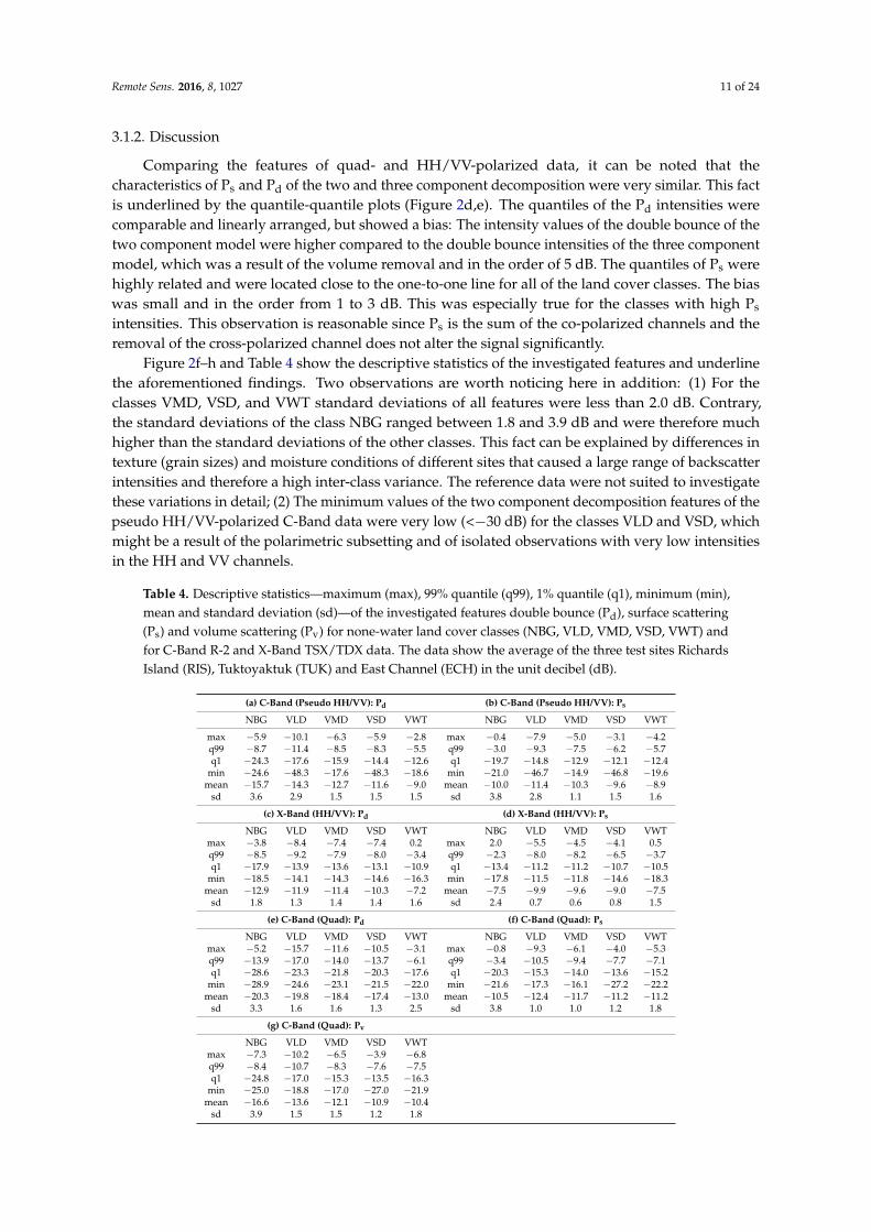
of compact polarimetric systems (exemplarily: [6,7]). However, there are fewer concepts on thedecomposition of dual-polarized data [8–10]. This type of PolSAR data advances higher spatialresolution and larger area coverage compared to the quad-polarized mode. Moreover, it offers highersignal-to-noise ratio (SNR) compared to the quad-pol data. Exemplarily, Cloude [8] showed theapplication of the mathematical, eigen-based Entropy/Alpha decomposition for dual polarimetricdata. Since most of today’s systems—like Radarsat-2 (R-2), Sentinel-1 or ALOS-2—provide onlyHH/HV- or VV/VH-polarized data operationally, most attention was paid on the analyses of thesetypes of dual-polarized data. With TerraSAR-X (TSX), TanDEM-X (TDX), and COSMO-Skymed anincreasing number of high resolution SAR systems is capable of acquiring HH/VV-polarized dataphase-coherently. Hence, co-polarimetric phase as well as amplitude information of the complex SARmeasurement is available for the analysis. Therefore, this kind of data also allows investigating thepolarimetric phase-relation between the HH and VV channels. This information is known to be animportant discriminator for the characterization of surface and double bounce scattering, respectivelyof odd and even bounce [1,5].

Studies that highlight the benefit and applicability of HH/VV-polarized data for land covercharacterization and classification are briefly named in the following. A decomposition scheme forHH/VV-polarized data was presented by Jagdhuber et al. [11,12] in the context of soil moistureestimation under agricultural vegetation. The approach utilizes a model-based volume componentremoval including the generation of synthetic cross-polarization (via the coherence of the complexHH and VV signals) and the dual-polarimetric eigen-based decomposition to retrieve the surface soilsignal. The phase-relation of HH and VV was also investigated by Lopez-Sanchez et al. [13], whoapplied an eigen-based decomposition to TerraSAR-X HH/VV-polarized data. The findings indicatedthe usefulness of these dual-polarized data for the characterization of the type of scattering that wasexamined in the context of time series analyses for the retrieval of rice phenology (surface or doublebounce scattering). Differences between the eigen-based decomposition features of HH/VV-polarizedcompared to quad-polarized data were investigated by [14]. Mitsunobu et al. [14] and showed astrong relation of the scattering angles. Voormansik et al. [15] investigated the potential of HH/VVdual-polarized TSX-data for studying grassland and to work towards the assessment of cuttingpractices on meadows. Heine et al. [16] used co-polarized TSX-data in time series for the analysisof phenological changes of wetland vegetation and showed that parameters sensitive to the doublebounce revealed meaningful seasonal changes for reed belts. Further, Schmitt et al. [17] examinedthe Entropy/Alpha and Freeman-Durden decomposition models, as well as, the elements of thenormalized Kennaugh Matrix of quad-polarized data for the characterization and classificationof wetland vegetation. The findings indicated that HH and VV information were crucial for thecharacterization and pointed to the high effectiveness and applicability of HH/VV-polarized data thatmaintain higher spatial resolution and coverage compared to quad-polarized data.

The application of SAR and PolSAR data has special relevance for Arctic environments since theapplication of multispectral, respectively optical imaging is limited in this region, due to the shortlength of the growing season and the rapid phenological seasonal response of the tundra vegetation.In this context the frequent cloud cover of the high latitudes hinders the acquisition of optical datasuited for time series analysis. A further challenge is the solar geometry: multispectral imaging isrestricted to the summer months when the illumination conditions cause a large range of zenith andazimuth angles that complicate the image analysis [18]. Even though active radar remote sensing canovercome most of these problems, there are comparably few studies that incorporate SAR/PolSARdata for land surface characterization of Arctic environment; exemplary [19–28]. Possible reasons forthis “lack of usage” are the difficult image interpretation, the unknown relation between SAR/PolSARscattering and Arctic land surface properties and the restricted access to the data. At least the last pointis becoming obsolete for C-Band SAR data with the operation of the Sentinel-1 satellites.

This study presents analyses of HH/VV-polarized data for the tundra environment of theMackenzie Delta Region, Canada using C-Band R-2 and X-Band TSX/TDX data. Special emphasis is

Remote Sens. 2016, 8, 1027 3 of 24

given on a two component, polarimetric decomposition of the dual-polarized data using a model thatis a straight forward adaption of the model purposed for quad-polarized data by Yamaguchi et al. [29].To our best knowledge such a straight forward adaptation of the Yamaguchi decomposition was nevertested for HH/VV SAR data, beside our preliminary experiments [26,30]. The aim is to enhancethe interpretability of the HH/VV SAR signal via the characterization of scattering mechanisms andto express the dual-polarized information in terms of scattering power components—similar to theFreeman-Durden and Yamaguchi decomposition models that are frequently applied to quad-polarizeddata. Further, its scope is to identify the benefit of polarimetry and to increase the understanding ofscattering and backscatter formation in tundra environment and to propose techniques that enablebetter and more accurate classifications of the Arctic land surface.

2. Materials and Methods

2.1. Two Component Decomposition of HH/VV Data

Working with coherent HH/VV-polarized data, information of both channels HH and VV maybe expressed by the coherency matrix T. The matrix is derived by multiplying the two componenttarget Pauli vector kτ (Equation (1)) with its conjugate transpose k+

τ (Equation (2)). T is a Hermitianmatrix with two by two elements (Equation (3)) and represents the upper square sub-matrix ofthe full 3 × 3 coherency matrix of a quad-polarized measurement. The matrix elements are linearcombinations of the complex HH- and VV-channels, based on the Pauli spin matrices [2] (Equation (4)).T can be used to exploit the phase difference of HH and VV channels: This relation is known to be acrucial discriminator for the characterization of the type of backscattering [1,31]; more precisely thediscrimination between odd- and even-bounce scattering.

kτ =1√2

(SHH + SVV

SHH − SVV

)(1)

T = kτk+τ =

[T11 T12

T21 T22

](2)

T =12〈[

(SHH + SVV)(SHH + SVV)∗ (SHH + SVV)(SHH − SVV)

∗

(SHH − SVV)(SHH + SVV)∗ (SHH − SVV)(SHH − SVV)

∗

]〉 (3)

In the formulas ∗ denotes the complex conjugate, + the conjugate transpose, and 〈〉 refersto the spatial averaging. Yamaguchi et al. [29] introduced a modified four component scatteringmodel for quad-polarized data based on the decomposition concept of Freeman and Durden [32].The approach of Yamaguchi et al. [29] is decomposing the full 3 × 3 coherency matrix into four signalcomponents of surface scattering, double bounce, volume, and helix scattering (so-called powercomponents). The method utilizes the model for the Bragg scattering via reflection coefficients thatrely on the co-polarized information alone. The coefficients of α and β are defined as stated inthe original approach of Yamaguchi et al. [29] and display the orientation and characteristic of thescattered wave [5], thus these coefficients contain the “polarimetric information” and are called the“scattering mechanisms”. The decomposition model of Yamaguchi et al. [29] can be realized as a threecomponent model, which is the more frequently applied approach. The model then decomposes the full3 × 3 coherency matrix T into the features surface, double bounce, and volume scattering. A straightforward adaption of this approach for HH/VV-polarized SAR data is the decomposition of the spaninto the scattering power components of surface (Ps) and double bounce (Pd) scattering neglectingvolume scattering: The estimation of these parameters is based on the co-polarized information

Remote Sens. 2016, 8, 1027 4 of 24

alone. Such a two component decomposition model can be designed assuming no contribution of thecross-polarized channels on the respective co-polarized channels as shown in Equations (5) and (6).

PT = Ps + Pd =

[T11 T12

T21 T22

]= fs

[1 β∗

β |β|2

]+ fd

[|α|2 α

α∗ 1

](4)

The definition of the model leads to the three equations shown in Equations (5)–(7). The equationsystem has four unknowns fs, fd, α, and β, and is therewith underdetermined. The unknowns fs andfd are the intensity components of the two scattering components to be determined [29]. The left handside is given by the measured values of T11, T12, T21, and T22 of the HH/VV-polarized CoherencyMatrix T.

T11 = 0.5〈|SHH + SVV|2〉 = fs + fd|α|2 (5)

T22 = 0.5〈|SHH − SVV|2〉 = fd + fs|β|2 (6)

T12 = 0.5〈(SHH + SVV)(SHH − SVV)∗〉 = fdα+ fsβ

∗ (7)

Two cases can be distinguished to simplify the equation system in order to be uniquely solvable;Case 1 with dominant surface scattering (T11 > T22 and α = 0) and Case 2, with dominant doublebounce scattering (T22 > T11 and β∗ = 0), where the non-dominant scattering contribution is set tozero [5]. These definitions are identical to the original models of Yamaguchi and Freeman-Durden. Theunknowns fs, fd, α or β are then defined by Equations (8)–(10) for Case 1 and by Equations (11)–(13)for Case 2.

Case 1: T11 > T22, with α = 0:fs = T11 (8)

fd = T22 −(|T12|2

T11

)(9)

β∗ =T12

T11(10)

Case 2: T22 > T11, with β∗ = 0:fd = T22 (11)

fs = T11 −(|T12|2

T22

)(12)

α =T12

T22(13)

The scattering power components Ps and Pd can be derived via Equations (14) and (15) consistentlyfor both cases:

Ps = fs(1 + |β|2) (14)

Pd = fd(1 + |α|2) (15)

The differences between the decomposition features of this two component model and of thethree component model of [29] are the assumption of the absence of a significant volume scatteringcontribution and a volume-induced depolarization, respectively. This means the cross-polarizedinformation will be ignored and is not measured for dual-polarimetric T. For real world applicationsone should take into account that a zero contribution of the cross-polarized channels—respectively anobservation of T33 = 0 in terms of quad-polarized coherency matrix—is not a likely situation for radarobservations of natural surfaces [1]. Furthermore, zero elements in the off-diagonal positions T13/31and T23/32 of quad-polarized coherency matrices are only observable when no coherence betweencross- and co-polarized channels is present [1] due to reflection symmetry for example. Nevertheless,this is a quite frequently applied symmetry assumption for natural media [5,29].

Remote Sens. 2016, 8, 1027 5 of 24

Accordingly, the correlations of Ps and Pd between the two and three component decompositionmodels is expected to be high for land cover types, e.g., bare or sparsely vegetated ground, that show nosignificant volume scattering with respect to the used wavelength and the spatial resolution. Contrary,the differences will be maximized for urban areas and for densely vegetated ground like forests:for such land cover types the contribution of volume scattering is usually high and not negligibleat all. In comparison to the simple Pauli decomposition the discrimination between double-bounce(or even bounce in Pauli’s definition) and surface scattering (or odd bounce in the Pauli notation) isenhanced by introducing the polarimetric scattering mechanisms α and β in Equations (14) and (15).The idea is to understand both, the intensity (fs, fd) and the scattering mechanisms (α, β) by usingalso the coherent nature of the data and not only the incoherent channel intensities (like for the Paulidecomposition of multi-looked images). Moreover, the Pauli decomposition would only distinguishbetween odd and even bounce scattering (multiple bounces) and not directly between surface anddouble-bounce scattering. So higher order scattering is actually not expected for tundra and just puresurface or dihedral scattering should be present, as the vegetation is low and comparably simple instructure. Thus, land cover discrimination and PolSAR signal interpretation is expected to be easierthan using just the simple elements of the Coherency matrix.

2.2. PolSAR Database

We investigated quad-polarized R-2 and HH/VV-polarized TSX/TDX data of the ArcticMackenzie Delta Region (Canada) in order to test the proposed decomposition approach and toexamine the PolSAR signal in relation to the land coverage. This Arctic region exhibits a variety ofland cover types on small scale and the transition between taiga and tundra ecosystems [33]. Figure 1shows the location of the site and field photographs of frequent land cover types. The PolSAR datawere acquired in Fine Mode (R-2), respectively Stripmap Mode (TSX/TDX), in the years 2010, 2011,and 2012. From the quad-polarized R-2 data we created pseudo HH/VV-polarized data as polarimetricsubsets taking the upper 2 × 2 square matrix of the quad-polarized coherency matrix. All PolSAR datawere processed to a ground range resolution of twelve meters using the Range-Doppler-Approachand intermediate TanDEM-X elevation model data (DEM) acquired in winter 2011/2012 with twelvemeter spatial resolution. Using this DEM the PolSAR data were calibrated to sigma nought (σ◦) viathe calibration factors and the sine of the local incidence angle derived from the TanDEM-X DEM.

No further processing was applied to the data but to the multi-looking and the subsequentboxcar/speckle filtering during the estimation of T with a window size of five by five pixels. All ofthe data were recorded with incidence angles between 31◦ and 46◦ during the summer months; snowand ice free conditions were present. Therefore temporal effects were not considered in the analysisand we assumed a minor role of land cover changes within the years 2010, 2012, and 2013 due to theslow pace of environmental transformation processes in these latitudes. Table 1 summarizes the mainparameters of the PolSAR database and names the location of the site.

Table 1. Acquisition parameters of TerraSAR-X (TSX), TanDEM-X (TDX) and Radarsat-2 (R-2).

Sensor Acquisition Date Acquisition Mode Polarization Incidence Angle (◦) Test Site Coverage 1

TDX 4 September 2012 Stripmap HH/VV 31.7 RISTSX 15 September 2012 Stripmap HH/VV 32.8 RISTSX 3 August 2011 Stripmap HH/VV 38.8 TUKTDX 4 September 2012 Stripmap HH/VV 31.7 ECHTSX 15 September 2012 Stripmap HH/VV 32.8 ECHR-2 5 August 2010 Fine HH/HV/VH/VV 46.1 RISR-2 25 August 2010 Fine HH/HV/VH/VV 40.7 RISR-2 19 August 2011 Fine HH/HV/VH/VV 40.5 TUKR-2 5 August 2010 Fine HH/HV/VH/VV 39.3 ECHR-2 25 August 2010 Fine HH/HV/VH/VV 39.0 ECH

1 RIS = Richards Island, TUK = Tuktoyaktuk, ECH = East Channel of the Mackenzie River.

Remote Sens. 2016, 8, 1027 6 of 24

Remote Sens. 2016, 8, 1027 6 of 24

Figure 1. Test site location: (a) Extent of the investigation areas, locations of the in situ field work and (b) field photographs of frequent land cover classes. The background map in (a) shows the topographic slope derived from intermediate TanDEM-X elevation model data provided by DLR (2012, German Aerospace Center); grey color indicates sloped terrain. Extents of the test sites refer to the common image footprints of the SAR acquisitions of TerraSAR-X/TanDEM-X and Radarsat-2.

2.3. In Situ Data

Additionally, in situ ground truth data on the land cover were recorded in the summers of the years 2010, 2012, and 2013. The location of the investigated sites is drawn in Figure 1. In 2010 the field work was conducted by the NWRC (National Wildlife Research Centre, Ottawa, ON, Canada). The field work in 2012 and 2013 was conducted by the Carleton University Ottawa, the NWRC, and the University of Wuerzburg. More than forty locations inside the region were visited and surface

Figure 1. Test site location: (a) Extent of the investigation areas, locations of the in situ field work and(b) field photographs of frequent land cover classes. The background map in (a) shows the topographicslope derived from intermediate TanDEM-X elevation model data provided by DLR (2012, GermanAerospace Center); grey color indicates sloped terrain. Extents of the test sites refer to the commonimage footprints of the SAR acquisitions of TerraSAR-X/TanDEM-X and Radarsat-2.

2.3. In Situ Data

Additionally, in situ ground truth data on the land cover were recorded in the summers of theyears 2010, 2012, and 2013. The location of the investigated sites is drawn in Figure 1. In 2010 thefield work was conducted by the NWRC (National Wildlife Research Centre, Ottawa, ON, Canada).The field work in 2012 and 2013 was conducted by the Carleton University Ottawa, the NWRC, andthe University of Wuerzburg. More than forty locations inside the region were visited and surfaceproperties were documented. The number of reference samples was increased afterwards usinghigh resolution aerial ortho-photos provided by Hartmann and Sachs [34] and NWT-Geomatics [35].

Remote Sens. 2016, 8, 1027 7 of 24

After this operation the set of land cover reference data comprised more than 1700 individual polygonsand a minimum of 200 polygons per land cover class. A set of 1000 points per class was then chosenrandomly for each test site.

Six land cover classes were distinguished qualitatively in the field (Table 2) and in dependence onthe classification systems of Corns [36] and the Land Cover Classification LCC-2000-V provided by theauthorities of the Natural Resources Canada (geogratis.gc.ca): Water, Bare Ground (NBG), Low/SparselyVegetated Tundra (VLD), Medium/Mixed Tundra (VMD), High/Shrub-Dominated Tundra (VSD),and Wetlands (VWT). The main cut-off criteria for the categorization of the land cover classes were theestimated height of the vegetation and the occurrence/density of the shrubs. Table 2 draws the mainparameters and a scheme of these generalized land cover classes. The sorting of the classes from NBGto VLD to VMD to VSD corresponds to increasing vegetation height and shrub density on an ordinalscale. Photographs of the classes VLD, VWT, and VSD are provided in Figure 1.

Table 2. Parameters, description, and scheme of the generalized land cover classes.

Class NameVWT NBG VLD VMD VSD

WetlandBare Substrate/Non-Vegetated

Ground

Low/Grass and HerbDominated Tundra

Medium/Mixed Tundra

High/ShrubDominated Tundra

Scheme

Remote Sens. 2016, 8, 1027 7 of 24

properties were documented. The number of reference samples was increased afterwards using high resolution aerial ortho-photos provided by Hartmann and Sachs [34] and NWT-Geomatics [35]. After this operation the set of land cover reference data comprised more than 1700 individual polygons and a minimum of 200 polygons per land cover class. A set of 1000 points per class was then chosen randomly for each test site.

Six land cover classes were distinguished qualitatively in the field (Table 2) and in dependence on the classification systems of Corns [36] and the Land Cover Classification LCC-2000-V provided by the authorities of the Natural Resources Canada (geogratis.gc.ca): Water, Bare Ground (NBG), Low/Sparsely Vegetated Tundra (VLD), Medium/Mixed Tundra (VMD), High/Shrub-Dominated Tundra (VSD), and Wetlands (VWT). The main cut-off criteria for the categorization of the land cover classes were the estimated height of the vegetation and the occurrence/density of the shrubs. Table 2 draws the main parameters and a scheme of these generalized land cover classes. The sorting of the classes from NBG to VLD to VMD to VSD corresponds to increasing vegetation height and shrub density on an ordinal scale. Photographs of the classes VLD, VWT, and VSD are provided in Figure 1.

Table 2. Parameters, description, and scheme of the generalized land cover classes.

Class Name

VWT NBG VLD VMD VSD

Wetland Bare Substrate/Non-Vegetated

Ground

Low/Grass and Herb Dominated Tundra

Medium/ Mixed Tundra

High/Shrub Dominated Tundra

Scheme

Description

vegetation in standing water dominated by reed and sedge

formations

exposed soil substrate and bedrock of varying grain sizes and material

open to closed vegetative cover dominated by

formations of grasses, mosses and herbs

closed vegetative cover dominated by formations of herbs and dwarf shrubs

closed vegetative cover dominated by formations of dwarf shrubs and shrubs

Vegetation Height

~10–50 cm n/a ~5–30 cm ~20–50 cm ~30–100 cm

Shrub Density

n/a n/a low moderate high

2.4. Correlation Analysis

The relationships and dependencies between the features of the two and three component decomposition were investigated for the C-Band and X-Band datasets using correlation analysis. The two component decomposition features Ps and Pd were processed for C-Band HH/VV-polarized data and X-Band HH/VV-polarized data. The three component decomposition features Ps, Pd, and Pv were processed using the C-Band quad-polarized data. The alterations between the C-Band two and three component decomposition features Ps (Pd) were then connected to the differences of the models and not to changes caused by temporal variations, since pseudo HH/VV-polarized data were derived from quad-polarized data. Table 3 provides an overview of the investigated features.

Table 3. Decomposition features examined in the correlation, regression, and separability analysis.

Feature Name Wavelength Polarization Decomposition Model P Double Bounce X-Band HH/VV Two Component P Surface Scattering X-Band HH/VV Two Component P Double Bounce C-Band HH/VV Two Component P Surface Scattering C-Band HH/VV Two Component P Double Bounce C-Band Quad Three Component P Surface Scattering C-Band Quad Three Component P Volume Scattering C-Band Quad Three Component

Description

vegetation instanding waterdominated by

reed and sedgeformations

exposed soilsubstrate and

bedrock of varyinggrain sizes and

material

open to closedvegetative cover

dominated byformations of grasses,

mosses and herbs

closed vegetativecover dominated byformations of herbsand dwarf shrubs

closed vegetativecover dominated byformations of dwarfshrubs and shrubs

VegetationHeight ~10–50 cm n/a ~5–30 cm ~20–50 cm ~30–100 cm

ShrubDensity n/a n/a low moderate high


The relationships and dependencies between the features of the two and three componentdecomposition were investigated for the C-Band and X-Band datasets using correlation analysis.The two component decomposition features Ps and Pd were processed for C-Band HH/VV-polarizeddata and X-Band HH/VV-polarized data. The three component decomposition features Ps, Pd, and Pv

were processed using the C-Band quad-polarized data. The alterations between the C-Band two andthree component decomposition features Ps (Pd) were then connected to the differences of the modelsand not to changes caused by temporal variations, since pseudo HH/VV-polarized data were derivedfrom quad-polarized data. Table 3 provides an overview of the investigated features.

Table 3. Decomposition features examined in the correlation, regression, and separability analysis.

Feature Name Wavelength Polarization Decomposition Model

Pd Double Bounce X-Band HH/VV Two ComponentPs Surface Scattering X-Band HH/VV Two ComponentPd Double Bounce C-Band HH/VV Two ComponentPs Surface Scattering C-Band HH/VV Two ComponentPd Double Bounce C-Band Quad Three ComponentPs Surface Scattering C-Band Quad Three ComponentPv Volume Scattering C-Band Quad Three Component

Remote Sens. 2016, 8, 1027 8 of 24

Prior to the analysis, a random stratification was applied to the land cover reference dataset toavoid auto-correlation: For each land cover class and each test site a set of 1000 pixels was chosenrandomly (see Section 2.3 in situ Data).

The correlations between the decomposition features were investigated using the intensity valuesof the sigma nought calibrated data. The linear Pearson Correlation Coefficient (R), the squaredlinear Pearson Correlation Coefficient (R2), and the Spearman’s Rank Correlation Coefficient (ρ) wereprocessed for all of the features for each land cover class of each test site using the reference data.The coefficient R is defined as the ratio between the covariance (Cov) of two variables (i,j) and theproduct of the individual standard deviations of these two variables (SD) (16) and (17). Similar, ρ isdefined as the ratio between the covariance (Cov) of two ranked variables (RGi, RGj) and the productof the individual standard deviations of these two ranked variables (σRGi σRGj ) (18).

SD =√

σiσj (16)

R =Cov(i, j)

SD2 (17)

ρ =Cov

(RGi, RGj

)σRGi σRGj

(18)

The coefficients R and ρ are relative and dimensionless and therefore show the linear (R)or monotonic (ρ) correlations among the features, respectively the degree of determination (R2).The values of R and R2 range from zero to one, where a value of one (zero) indicates perfect (no)linear correlation and a maximum (minimum) determination, which is 100% (0%) of the explainedvariance. The values of ρ range from −1 to +1, where −1/+1 indicate perfect monotonic properties,thus one variable is a function of the other. R and ρ were investigated to examine the linear andmonotonic dependencies among the features. The X-Band data acted as a control variable in thisstudy: A positive correlation between C- and X-Band is expected due to the similar wavelengths of5 cm and 3 cm, respectively. However; this relationship should be less significant compared to thecorrelation among the C-Band features due to the temporal decorrelation, the differences in the specklecharacteristics, and the differences in absolute radiometric calibration. Therefore it is more statisticallyreliable to compare C-Band quad-polarized with C-Band synthesized dual-polarized data.

2.5. Regression Analysis

Along with the correlation coefficients, the parameters of the linear regression models wereprocessed for all of the features for each land cover class of each test site using the reference data.The linear model y = ax + b was assumed for the modelling. The two linear model parameters are theslope (coefficient a) and the axis intercept (coefficient b). The differences between the predictions (y)and the true observations (y’) can be expressed via the Root Mean Square Error (RMSE). The RMSE(Equation (19)) is an absolute measurement of the mean deviation of the model and processed for asample n. It is therefore measured in the unit of the input variables—decibel (dB) in our case, since thescattering power components were investigated. The RMSE is a frequently used measure to assessthe absolute variation of the model prediction, which is often interpreted as the “absolute error” ofthe model.

RMSE =

√∑n

t=1(yt − y′t)2

n(19)

RMSE is not adjusted to the variances of the two samples (SD) and it should therefore beinterpreted along with a relative correlation coefficient, or with a feature that displays the variations ofthe features (e.g., SD). A low (high) coefficient of determination (R2) does not necessarily infer a high(low) RMSE, e.g., in the case that the classes’ standard deviations are low (high).

Remote Sens. 2016, 8, 1027 9 of 24

2.6. Separability Analysis

The separability features Jeffries Matusita Distance (JD) and Transformed Divergence (TD) [37,38]were further investigated to examine the differences between C- and X-Band, between the two andthree component decomposition features and to examine if PolSAR decomposition offers betterclass separation compared to the “pure” intensities of the polarimetric channels. The values of thedimensionless JD range from 0.0 to

√2. The values of the dimensionless Transformed Divergence

range usually from 0 to 2000. The higher the value of a separability feature the higher is the estimatedseparation of the classes in the feature space and the expected classification accuracy. JD and TDrequire that the values of the classes are normally distributed. This is usually not the case; however acommon assumption for natural targets and media for simplicity reasons. JD and TD then estimate theoverlap between the multivariate normal distributions of two classes of interest in a given feature space.Less (more) overlap indicates better (worse) separability and therefore the classification accuracy isexpected to be higher (lower).

The TD between two classes c and d is defined by Equation (20) using the classes’ mean vectorsM and the classes’ covariances V for a given set of features, with two features required as minimum.In the formula tr denotes the trace of a matrix and T refers to the matrix/vector transpose. C is a3 × 3 matrix and M a three-element vector for the case that three features are investigated [37].

TD = 2000

1− exp

−0.5(tr[(Vc − Vd)

(V−1

d − V−1c

)]+ tr[

(V−1

c + V−1d

)(Mc − Md)(Mc − Md)

T ])

8

(20)

The JD between two classes c and d is defined by (21) and (22) using the classes’ mean vectorsM and the classes’ covariances V for a given set of features, with two features required as minimum.The calculation of JD is based on the Bhattacharyya Distance (BD) (21). In the formula det denotes thedeterminant of a matrix. Both features are based on the Mahalanobis Distance, which estimates thedistance between a point and a distribution [37].

BD = 0.125(Mc −Md)T0.5(Vc + Vd)(Mc −Md) + 0.5loge

det(0.5(Vc + Vd))√det(Vc)

√det(Vd)

(21)

JD =√

2(1− e−BD) (22)

JD and TD were shown to act as authentic predictors for the accuracy of supervised classifications,when the classifier relies on normal distribution parametrization [37–39], e.g., the relationship betweenJM and supervised classification accuracy obtained from Maximum Likelihood Classification (based onthe Mahalanobis Distance). However, the saturation behavior of both features is different and thusit is meaningful to compute and to interpret both in the separability analysis. For this study theland cover reference data were used to define the classes’ statistics. The feature spaces examinedwere the intensities of C-Band pseudo dual-polarized data (HH/HV; VV/VH; HH/VV), C-Bandquad-polarized data (HH/HV/VV), X-Band dual-polarized data (HH/VV), C-Band Three ComponentDecomposition Features (Ps/Pd/Pv), C-Band Three Component Decomposition Features withoutthe volume scattering (Ps/Pd), C-Band Two Component Decomposition Features (Ps/Pd), and theX-Band Two Component Decomposition Features (Ps/Pd) (Table 3). The analysis was conducted forthe none-water land cover classes (NBG, VLD, VMD, VSD, VWT) to avoid an overestimation of theaverage separability; the class water is comparably easy to be classified with PolSAR data [31] and ahigh separability of this class might artificially enhance the results.

Remote Sens. 2016, 8, 1027 10 of 24

3. Results and Discussion

3.1. Backscatter Analysis

3.1.1. Results

The backscatter characteristics and descriptive statistics of the land cover classes were investigatedprior to the correlation, regression, and separability analyses. Figure 2 shows the medians of thecalibrated sigma nought backscatter intensities of the two and three component decomposition featuresin decibel for each land cover class and the X- and C-Band data. It can be noted that the double bounceintensities Pd are increasing for all features from NBG to VWT (Figure 2a). Contrary, all Ps intensitiesshowed similar value ranges and median values of the vegetation classes (VLD, VMD, VSD) weresimilar (Figure 2b). The volume scattering Pv of the three component decomposition model showedthe most variable value ranges and increasing intensities from NBG to VWT (Figure 2c). Pd and Pv canbe considered to be most meaningful for the class characterization and increasing volume scattering,respectively double bounce: The intensities increase with increasing vegetation height and shrubdensity (from NBG to VLD to VMD to VSD—see Section 2.3 in situ Data).

Remote Sens. 2016, 8, 1027 10 of 24

of the calibrated sigma nought backscatter intensities of the two and three component decomposition features in decibel for each land cover class and the X- and C-Band data. It can be noted that the double bounce intensities Pd are increasing for all features from NBG to VWT (Figure 2a). Contrary, all Ps intensities showed similar value ranges and median values of the vegetation classes (VLD, VMD, VSD) were similar (Figure 2b). The volume scattering Pv of the three component decomposition model showed the most variable value ranges and increasing intensities from NBG to VWT (Figure 2c). Pd and Pv can be considered to be most meaningful for the class characterization and increasing volume scattering, respectively double bounce: The intensities increase with increasing vegetation height and shrub density (from NBG to VLD to VMD to VSD—see Section 2.3 in situ Data).

Figure 2. Median sigma nought (σ°) backscatter intensities in decibel (dB) of: (a) double bounce (Pd), (b) surface scattering (Ps) and (c) volume scattering (Pv) for none-water land cover classes (NBG, VLD, VMD, VSD, VWT) and for C-Band Radarsat-2 and X-Band TerraSAR-X data. The power decomposition features of “C-Band: HH/VV” and “X-Band: HH/VV” were derived via the purposed two component decomposition. Features of “C-Band: Quad” were calculated using the three component Yamaguchi Decomposition. Schemes (d) and (e) show the quantile-quantile plots of the two and three component decomposition features double bounce (Pd) and surface scattering (Ps) for the quantiles 1%, 25%, 50%, 75%, and 99%. The boxplots show the decomposition features of: (f) C-Band: Quad; (g) C-Band: HH/VV and (h) X-Band: HH/VV. Note that NBG, VLD, VMD, and VSD are in an ordinal scale and vegetation height and density is increasing from NBG to VSD.

3.1.2. Discussion

Comparing the features of quad- and HH/VV-polarized data, it can be noted that the characteristics of Ps and Pd of the two and three component decomposition were very similar. This fact is underlined by the quantile-quantile plots (Figure 2d,e). The quantiles of the Pd intensities were

Figure 2. Median sigma nought (σ◦) backscatter intensities in decibel (dB) of: (a) double bounce (Pd),(b) surface scattering (Ps) and (c) volume scattering (Pv) for none-water land cover classes (NBG, VLD,VMD, VSD, VWT) and for C-Band Radarsat-2 and X-Band TerraSAR-X data. The power decompositionfeatures of “C-Band: HH/VV” and “X-Band: HH/VV” were derived via the purposed two componentdecomposition. Features of “C-Band: Quad” were calculated using the three component YamaguchiDecomposition. Schemes (d) and (e) show the quantile-quantile plots of the two and three componentdecomposition features double bounce (Pd) and surface scattering (Ps) for the quantiles 1%, 25%, 50%,75%, and 99%. The boxplots show the decomposition features of: (f) C-Band: Quad; (g) C-Band:HH/VV and (h) X-Band: HH/VV. Note that NBG, VLD, VMD, and VSD are in an ordinal scale andvegetation height and density is increasing from NBG to VSD.

Remote Sens. 2016, 8, 1027 11 of 24

3.1.2. Discussion

Comparing the features of quad- and HH/VV-polarized data, it can be noted that thecharacteristics of Ps and Pd of the two and three component decomposition were very similar. This factis underlined by the quantile-quantile plots (Figure 2d,e). The quantiles of the Pd intensities werecomparable and linearly arranged, but showed a bias: The intensity values of the double bounce of thetwo component model were higher compared to the double bounce intensities of the three componentmodel, which was a result of the volume removal and in the order of 5 dB. The quantiles of Ps werehighly related and were located close to the one-to-one line for all of the land cover classes. The biaswas small and in the order from 1 to 3 dB. This was especially true for the classes with high Ps

intensities. This observation is reasonable since Ps is the sum of the co-polarized channels and theremoval of the cross-polarized channel does not alter the signal significantly.

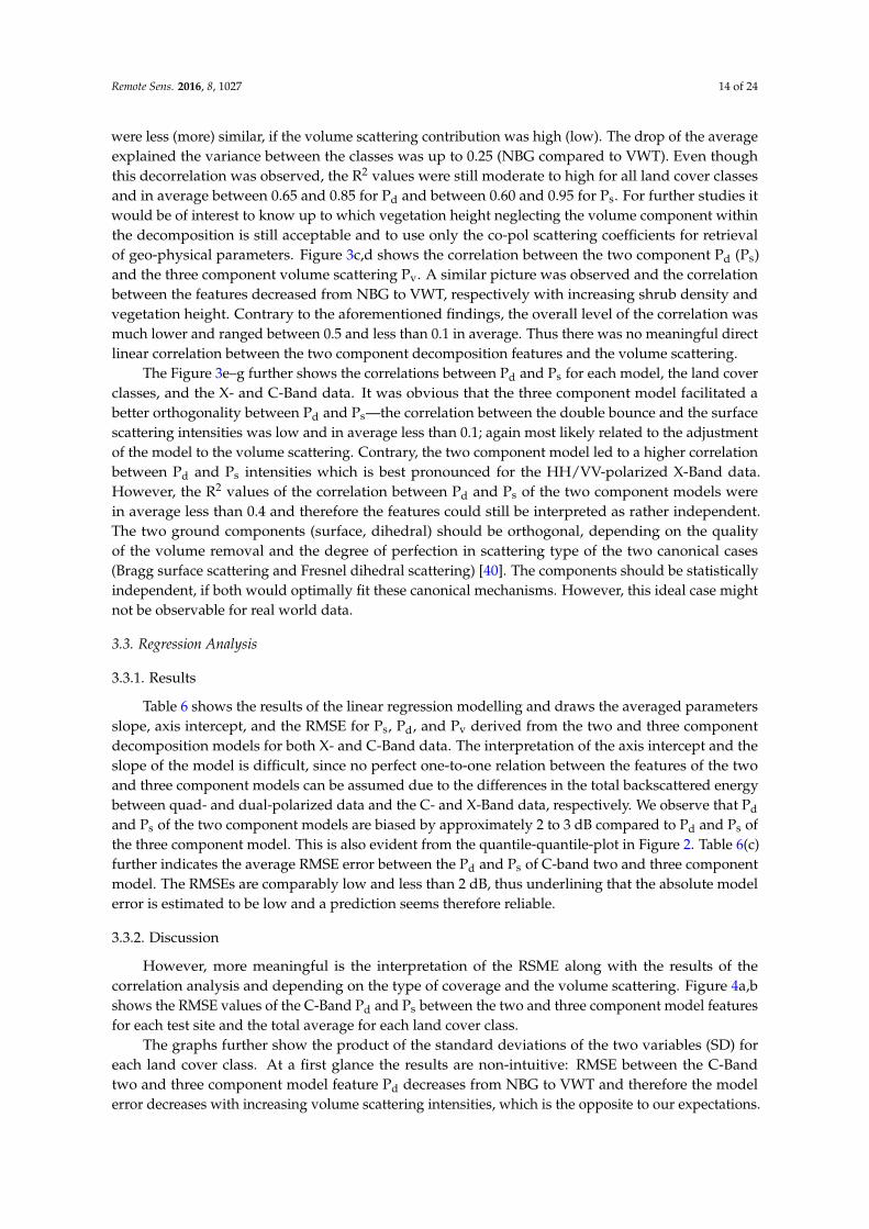
Figure 2f–h and Table 4 show the descriptive statistics of the investigated features and underlinethe aforementioned findings. Two observations are worth noticing here in addition: (1) For theclasses VMD, VSD, and VWT standard deviations of all features were less than 2.0 dB. Contrary,the standard deviations of the class NBG ranged between 1.8 and 3.9 dB and were therefore muchhigher than the standard deviations of the other classes. This fact can be explained by differences intexture (grain sizes) and moisture conditions of different sites that caused a large range of backscatterintensities and therefore a high inter-class variance. The reference data were not suited to investigatethese variations in detail; (2) The minimum values of the two component decomposition features of thepseudo HH/VV-polarized C-Band data were very low (<−30 dB) for the classes VLD and VSD, whichmight be a result of the polarimetric subsetting and of isolated observations with very low intensitiesin the HH and VV channels.

Table 4. Descriptive statistics—maximum (max), 99% quantile (q99), 1% quantile (q1), minimum (min),mean and standard deviation (sd)—of the investigated features double bounce (Pd), surface scattering(Ps) and volume scattering (Pv) for none-water land cover classes (NBG, VLD, VMD, VSD, VWT) andfor C-Band R-2 and X-Band TSX/TDX data. The data show the average of the three test sites RichardsIsland (RIS), Tuktoyaktuk (TUK) and East Channel (ECH) in the unit decibel (dB).

(a) C-Band (Pseudo HH/VV): Pd (b) C-Band (Pseudo HH/VV): Ps

NBG VLD VMD VSD VWT NBG VLD VMD VSD VWT

max −5.9 −10.1 −6.3 −5.9 −2.8 max −0.4 −7.9 −5.0 −3.1 −4.2q99 −8.7 −11.4 −8.5 −8.3 −5.5 q99 −3.0 −9.3 −7.5 −6.2 −5.7q1 −24.3 −17.6 −15.9 −14.4 −12.6 q1 −19.7 −14.8 −12.9 −12.1 −12.4

min −24.6 −48.3 −17.6 −48.3 −18.6 min −21.0 −46.7 −14.9 −46.8 −19.6mean −15.7 −14.3 −12.7 −11.6 −9.0 mean −10.0 −11.4 −10.3 −9.6 −8.9

sd 3.6 2.9 1.5 1.5 1.5 sd 3.8 2.8 1.1 1.5 1.6

(c) X-Band (HH/VV): Pd (d) X-Band (HH/VV): Ps

NBG VLD VMD VSD VWT NBG VLD VMD VSD VWTmax −3.8 −8.4 −7.4 −7.4 0.2 max 2.0 −5.5 −4.5 −4.1 0.5q99 −8.5 −9.2 −7.9 −8.0 −3.4 q99 −2.3 −8.0 −8.2 −6.5 −3.7q1 −17.9 −13.9 −13.6 −13.1 −10.9 q1 −13.4 −11.2 −11.2 −10.7 −10.5

min −18.5 −14.1 −14.3 −14.6 −16.3 min −17.8 −11.5 −11.8 −14.6 −18.3mean −12.9 −11.9 −11.4 −10.3 −7.2 mean −7.5 −9.9 −9.6 −9.0 −7.5

sd 1.8 1.3 1.4 1.4 1.6 sd 2.4 0.7 0.6 0.8 1.5

(e) C-Band (Quad): Pd (f) C-Band (Quad): Ps

NBG VLD VMD VSD VWT NBG VLD VMD VSD VWTmax −5.2 −15.7 −11.6 −10.5 −3.1 max −0.8 −9.3 −6.1 −4.0 −5.3q99 −13.9 −17.0 −14.0 −13.7 −6.1 q99 −3.4 −10.5 −9.4 −7.7 −7.1q1 −28.6 −23.3 −21.8 −20.3 −17.6 q1 −20.3 −15.3 −14.0 −13.6 −15.2

min −28.9 −24.6 −23.1 −21.5 −22.0 min −21.6 −17.3 −16.1 −27.2 −22.2mean −20.3 −19.8 −18.4 −17.4 −13.0 mean −10.5 −12.4 −11.7 −11.2 −11.2

sd 3.3 1.6 1.6 1.3 2.5 sd 3.8 1.0 1.0 1.2 1.8

(g) C-Band (Quad): Pv

NBG VLD VMD VSD VWTmax −7.3 −10.2 −6.5 −3.9 −6.8q99 −8.4 −10.7 −8.3 −7.6 −7.5q1 −24.8 −17.0 −15.3 −13.5 −16.3

min −25.0 −18.8 −17.0 −27.0 −21.9mean −16.6 −13.6 −12.1 −10.9 −10.4

sd 3.9 1.5 1.5 1.2 1.8

Remote Sens. 2016, 8, 1027 12 of 24


3.2.1. Results

Table 5 shows the averaged correlation coefficients between Ps, Pd, and Pv that were derivedusing the two and three component decomposition models for both X- and C-Band data. For all of thetest sites and features positive linear correlations (R > 0) and medium to high positive monotonies(ρ > 0.3) were observed. The correlations between the X- and C-Band features were very low andthe values of the squared Pearson Correlation Coefficients (R2) were less than 0.27. This is mostlikely a result of the different wavelengths and the temporal gap between the acquisitions. Further,no meaningful correlations between the volume scattering and any other feature were observed: All ofthe R2 values were less than 0.46, which points to the expected statistically independence of thedifferent polarizations. Contrary, the correlation between C-Band surface scattering features Ps of thetwo and three component models were high (R2 = 0.88) and monotone (ρ = 0.91).

Table 5. Average Pearson (a), squared Pearson (b) and Spearman (c) correlation coefficients of C-BandRadarsat-2 and X-Band TerraSAR-X data for two and three component decomposition features doublebounce (Pd), surface scattering (Ps), and volume scattering (Pv).

(a) Pearson (R)—Linear Dependence

Pd Ps Pv

X-HH/VV C-HH/VV C-Quad X-HH/VV C-HH/VV C-Quad C-Quad

1.00 0.52 0.42 0.20 0.45 0.36 0.47 X-HH/VVPd1.00 0.83 0.14 0.14 0.10 0.68 C-HH/VV

1.00 0.10 0.47 0.57 0.35 C-Quad

1.00 0.14 0.10 0.10 X-HH/VVPs1.00 0.94 0.64 C-HH/VV

1.00 0.46 C-Quad

1.00 C-Quad Pv

(b) Squared Pearson (R2)—Explained Variance

Pd Ps Pv


1.00 0.27 0.18 0.04 0.20 0.13 0.22 X-HH/VVPd1.00 0.69 0.02 0.02 0.01 0.46 C-HH/VV

1.00 0.01 0.22 0.32 0.12 C-Quad

1.00 0.02 0.01 0.01 X-HH/VVPs1.00 0.88 0.41 C-HH/VV

1.00 0.21 C-Quad

1.00 C-Quad Pv

(c) Spearman (ρ)—Monotonic Dependence

Pd Ps Pv


1.00 0.62 0.53 0.64 0.60 0.49 0.61 X-HH/VVPd1.00 0.84 0.38 0.67 0.54 0.78 C-HH/VV

1.00 0.33 0.55 0.48 0.53 C-Quad

1.00 0.44 0.38 0.39 X-HH/VVPs1.00 0.91 0.68 C-HH/VV

1.00 0.51 C-Quad

1.00 C-Quad Pv

Similarly, the correlation between C-Band double bounce features Pd of the two and threecomponent models were moderately high (R2 = 0.69) and monotone (ρ = 0.84). It is of importance tonotice that the correlation between Pd and Ps of the two component model is higher than the correlationbetween Pd and Ps of the three component model. This fact points to a weaker orthogonality of the

Remote Sens. 2016, 8, 1027 13 of 24

features of the two component decomposition model, which appears reasonable due to the missingremoval of volume scattering, that is potentially present in both components. In the following thecorrelation of Pd and Ps between both models was studied for each test site, taking the influence of theland cover into account. Figure 3a,b shows the R2 values of the C-Band Pd, and Ps between the two andthree component model features for each test site and the average for each land cover class. It wasfound that the R2 values between two and three component Pd (Ps) decreased from NBG to VWT.

Remote Sens. 2016, 8, 1027 13 of 24

cover class. It was found that the R2 values between two and three component Pd (Ps) decreased from NBG to VWT.

Figure 3. Squared linear Pearson correlation coefficients (R2) for none-water land cover classes (NBG, VLD, VMD, VSD, VWT) of: (a) double bounce (Pd) of the two and three component decomposition; (b) surface scattering (Ps) of the two and three component decomposition; (c) volume scattering (Pv) of three and Pd of the two component decomposition (C-Band); (d) Pv of three and Ps of the two component decomposition (C-Band); (e) Pd and Ps of the two component decomposition (C-Band); (f) Pd and Ps of the three component decomposition (C-Band) and (g) Pd and Ps of the two component decomposition (X-Band). Abbreviations of the test sites: TUK: Tuktoyaktuk, RIS: Richards Island, ECH: East Channel of the Mackenzie River.

3.2.2. Discussion

The decrease in correlation between between two and three component Pd (Ps) is likely due to the increase in volume scattering that was present from NBG to VWT (Figure 2) and a result of the increasing shrub density and vegetation height (Table 2). Thus, the features of the two decompositions were less (more) similar, if the volume scattering contribution was high (low). The drop of the average explained the variance between the classes was up to 0.25 (NBG compared to VWT). Even though this decorrelation was observed, the R2 values were still moderate to high for all land cover classes and in average between 0.65 and 0.85 for Pd and between 0.60 and 0.95 for Ps. For further studies it would be of interest to know up to which vegetation height neglecting the volume

Figure 3. Squared linear Pearson correlation coefficients (R2) for none-water land cover classes (NBG,VLD, VMD, VSD, VWT) of: (a) double bounce (Pd) of the two and three component decomposition;(b) surface scattering (Ps) of the two and three component decomposition; (c) volume scattering(Pv) of three and Pd of the two component decomposition (C-Band); (d) Pv of three and Ps of thetwo component decomposition (C-Band); (e) Pd and Ps of the two component decomposition (C-Band);(f) Pd and Ps of the three component decomposition (C-Band) and (g) Pd and Ps of the two componentdecomposition (X-Band). Abbreviations of the test sites: TUK: Tuktoyaktuk, RIS: Richards Island,ECH: East Channel of the Mackenzie River.

3.2.2. Discussion

The decrease in correlation between between two and three component Pd (Ps) is likely due tothe increase in volume scattering that was present from NBG to VWT (Figure 2) and a result of theincreasing shrub density and vegetation height (Table 2). Thus, the features of the two decompositions

Remote Sens. 2016, 8, 1027 14 of 24

were less (more) similar, if the volume scattering contribution was high (low). The drop of the averageexplained the variance between the classes was up to 0.25 (NBG compared to VWT). Even thoughthis decorrelation was observed, the R2 values were still moderate to high for all land cover classesand in average between 0.65 and 0.85 for Pd and between 0.60 and 0.95 for Ps. For further studies itwould be of interest to know up to which vegetation height neglecting the volume component withinthe decomposition is still acceptable and to use only the co-pol scattering coefficients for retrievalof geo-physical parameters. Figure 3c,d shows the correlation between the two component Pd (Ps)and the three component volume scattering Pv. A similar picture was observed and the correlationbetween the features decreased from NBG to VWT, respectively with increasing shrub density andvegetation height. Contrary to the aforementioned findings, the overall level of the correlation wasmuch lower and ranged between 0.5 and less than 0.1 in average. Thus there was no meaningful directlinear correlation between the two component decomposition features and the volume scattering.

The Figure 3e–g further shows the correlations between Pd and Ps for each model, the land coverclasses, and the X- and C-Band data. It was obvious that the three component model facilitated abetter orthogonality between Pd and Ps—the correlation between the double bounce and the surfacescattering intensities was low and in average less than 0.1; again most likely related to the adjustmentof the model to the volume scattering. Contrary, the two component model led to a higher correlationbetween Pd and Ps intensities which is best pronounced for the HH/VV-polarized X-Band data.However, the R2 values of the correlation between Pd and Ps of the two component models werein average less than 0.4 and therefore the features could still be interpreted as rather independent.The two ground components (surface, dihedral) should be orthogonal, depending on the qualityof the volume removal and the degree of perfection in scattering type of the two canonical cases(Bragg surface scattering and Fresnel dihedral scattering) [40]. The components should be statisticallyindependent, if both would optimally fit these canonical mechanisms. However, this ideal case mightnot be observable for real world data.

3.3. Regression Analysis

3.3.1. Results

Table 6 shows the results of the linear regression modelling and draws the averaged parametersslope, axis intercept, and the RMSE for Ps, Pd, and Pv derived from the two and three componentdecomposition models for both X- and C-Band data. The interpretation of the axis intercept and theslope of the model is difficult, since no perfect one-to-one relation between the features of the twoand three component models can be assumed due to the differences in the total backscattered energybetween quad- and dual-polarized data and the C- and X-Band data, respectively. We observe that Pdand Ps of the two component models are biased by approximately 2 to 3 dB compared to Pd and Ps ofthe three component model. This is also evident from the quantile-quantile-plot in Figure 2. Table 6(c)further indicates the average RMSE error between the Pd and Ps of C-band two and three componentmodel. The RMSEs are comparably low and less than 2 dB, thus underlining that the absolute modelerror is estimated to be low and a prediction seems therefore reliable.

3.3.2. Discussion

However, more meaningful is the interpretation of the RSME along with the results of thecorrelation analysis and depending on the type of coverage and the volume scattering. Figure 4a,bshows the RMSE values of the C-Band Pd and Ps between the two and three component model featuresfor each test site and the total average for each land cover class.

The graphs further show the product of the standard deviations of the two variables (SD) foreach land cover class. At a first glance the results are non-intuitive: RMSE between the C-Bandtwo and three component model feature Pd decreases from NBG to VWT and therefore the modelerror decreases with increasing volume scattering intensities, which is the opposite to our expectations.

Remote Sens. 2016, 8, 1027 15 of 24

However, the reason for this observation is the weak linear correlation between the features for thevegetation classes (Figure 3a). Therefore the RMSE becomes a function of the standard deviations ofthe two variables (SD; see Section 2.4 Regression Analysis), as it is obvious in the graph (compareTable 4 as well). Thus, the behavior of the RMSE can be explained by the SD values, which is alsotrue in Figure 4c–f and partially in Figure 4a for the classes VMD, VSD, and VWT. Figure 5 shows theobservations of Figures 3 and 4 in a scatterplot. The RMSE is drawn on the abscissa and the explainedvariance (R2) on the ordinate. This plot summarizes the findings made in the aforementioned sections.

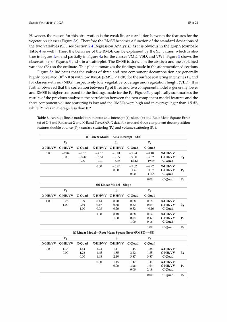
Figure 5a indicates that the values of three and two component decomposition are generallyhighly correlated (R2 > 0.8) with low RMSE (RMSE < 1 dB) for the surface scattering intensities Ps andfor classes with no (NBG), respectively low vegetative coverage and vegetation height (VLD). It isfurther observed that the correlation between Pd of three and two component model is generally lowerand RMSE is higher compared to the findings made for the Ps. Figure 5b graphically summarizes theresults of the previous analyses: the correlation between the two component model features and thethree component volume scattering is low and the RMSEs were high and in average lager than 1.5 dB,while R2 was in average less than 0.2.

Table 6. Average linear model parameters: axis intercept (a), slope (b) and Root Mean Square Error(c) of C-Band Radarsat-2 and X-Band TerraSAR-X data for two and three component decompositionfeatures double bounce (Pd), surface scattering (Ps) and volume scattering (Pv).

(a) Linear Model—Axis Intercept—(dB)

Pd Ps Pv


0.00 −7.84 −9.15 −7.15 −8.74 −9.94 −8.48 X-HH/VVPd0.00 −3.42 −6.51 −7.19 −9.30 −5.32 C-HH/VV

0.00 −7.30 −5.98 −15.42 −19.69 C-Quad

0.00 −6.95 −7.82 −6.92 X-HH/VVPs0.00 −2.46 −3.87 C-HH/VV

0.00 −11.05 C-Quad

0.00 C-Quad Pv

(b) Linear Model—Slope

Pd Ps Pv


1.00 0.23 0.09 0.44 0.20 0.08 0.18 X-HH/VVPd1.00 0.49 0.17 0.58 0.32 0.59 C-HH/VV

1.00 0.08 0.20 0.32 −0.10 C-Quad

1.00 0.18 0.08 0.14 X-HH/VVPs1.00 0.64 0.47 C-HH/VV

1.00 0.16 C-Quad

1.00 C-Quad Pv

(c) Linear Model—Root Mean Square Error (RMSE)—(dB)

Pd Ps Pv


0.00 1.38 1.44 1.24 1.41 1.45 1.38 X-HH/VVPd0.00 1.78 1.45 1.85 2.22 1.85 C-HH/VV

0.00 1.48 2.10 3.87 3.87 C-Quad

0.00 1.45 1.47 1.44 X-HH/VVPs0.00 1.05 1.64 C-HH/VV

0.00 2.19 C-Quad

0.00 C-Quad Pv

Remote Sens. 2016, 8, 1027 16 of 24Remote Sens. 2016, 8, 1027 16 of 24

Figure 4. Root Mean Square Error (RMSE) of the linear models and the product of standard deviations of the two variables (SD) for none-water land cover classes (NBG, VLD, VMD, VSD, VWT) for: (a) double bounce (Pd) of the two and three component decomposition; (b) surface scattering (Ps) of the two and three component decomposition; (c) volume scattering (Pv) of three and Pd of the two component decomposition (C-Band); (d) Pv of three and Ps of the two component decomposition (C-Band); (e) Pd and Ps of the two component decomposition (C-Band); (f) Pd and Ps of the three component decomposition (C-Band) and (g) Pd and Ps of the two component decomposition (X-Band). Note the different value range of the ordinate in sub-figure (f). Abbreviations of the test sites: TUK: Tuktoyaktuk, RIS: Richards Island, ECH: East Channel of the Mackenzie River.

Figure 5. Averaged Squared Linear Pearson Correlation Coefficients (R2) for none-water land cover classes (NBG, VLD, VMD, VSD, VWT) versus the Averaged Root Mean Square Errors (RMSE) of the linear models for C-Band features: (a) double bounce (Pd) and surface scattering (Ps) of the two and three component decomposition; (b) volume scattering (Pv). double bounce (Pd), and surface scattering (Ps) of the two component decomposition.

Figure 4. Root Mean Square Error (RMSE) of the linear models and the product of standard deviations ofthe two variables (SD) for none-water land cover classes (NBG, VLD, VMD, VSD, VWT) for: (a) doublebounce (Pd) of the two and three component decomposition; (b) surface scattering (Ps) of the two andthree component decomposition; (c) volume scattering (Pv) of three and Pd of the two componentdecomposition (C-Band); (d) Pv of three and Ps of the two component decomposition (C-Band);(e) Pd and Ps of the two component decomposition (C-Band); (f) Pd and Ps of the three componentdecomposition (C-Band) and (g) Pd and Ps of the two component decomposition (X-Band). Note thedifferent value range of the ordinate in sub-figure (f). Abbreviations of the test sites: TUK: Tuktoyaktuk,RIS: Richards Island, ECH: East Channel of the Mackenzie River.

Remote Sens. 2016, 8, 1027 16 of 24

Figure 4. Root Mean Square Error (RMSE) of the linear models and the product of standard deviations of the two variables (SD) for none-water land cover classes (NBG, VLD, VMD, VSD, VWT) for: (a) double bounce (Pd) of the two and three component decomposition; (b) surface scattering (Ps) of the two and three component decomposition; (c) volume scattering (Pv) of three and Pd of the two component decomposition (C-Band); (d) Pv of three and Ps of the two component decomposition (C-Band); (e) Pd and Ps of the two component decomposition (C-Band); (f) Pd and Ps of the three component decomposition (C-Band) and (g) Pd and Ps of the two component decomposition (X-Band). Note the different value range of the ordinate in sub-figure (f). Abbreviations of the test sites: TUK: Tuktoyaktuk, RIS: Richards Island, ECH: East Channel of the Mackenzie River.

Figure 5. Averaged Squared Linear Pearson Correlation Coefficients (R2) for none-water land cover classes (NBG, VLD, VMD, VSD, VWT) versus the Averaged Root Mean Square Errors (RMSE) of the linear models for C-Band features: (a) double bounce (Pd) and surface scattering (Ps) of the two and three component decomposition; (b) volume scattering (Pv). double bounce (Pd), and surface scattering (Ps) of the two component decomposition.

Figure 5. Averaged Squared Linear Pearson Correlation Coefficients (R2) for none-water land coverclasses (NBG, VLD, VMD, VSD, VWT) versus the Averaged Root Mean Square Errors (RMSE) of thelinear models for C-Band features: (a) double bounce (Pd) and surface scattering (Ps) of the two andthree component decomposition; (b) volume scattering (Pv). double bounce (Pd), and surface scattering(Ps) of the two component decomposition.

Remote Sens. 2016, 8, 1027 17 of 24


3.4.1. Results

In the following the effect of two and/or three component decomposition on the separabilityof classes in the feature space was investigated (see Section 2.6 Separability Analysis). Figure 6shows the results of the assessment for the non-water land cover classes. Figure 6a,b displays theresults obtained with polarimetric decomposition. Figure 6c,d displays the results obtained withoutpolarimetric decomposition—that means that only the intensities of the polarimetric channels wereused in the separability analysis. The results are further displayed for the JM (left side) and the TD(right side); however, differences between JD and TD were small and restricted to individual classesand feature combinations.

Remote Sens. 2016, 8, 1027 17 of 24


3.4.1. Results

In the following the effect of two and/or three component decomposition on the separability of classes in the feature space was investigated (see Section 2.6 Separability Analysis). Figure 6 shows the results of the assessment for the non-water land cover classes. Figure 6a,b displays the results obtained with polarimetric decomposition. Figure 6c,d displays the results obtained without polarimetric decomposition—that means that only the intensities of the polarimetric channels were used in the separability analysis. The results are further displayed for the JM (left side) and the TD (right side); however, differences between JD and TD were small and restricted to individual classes and feature combinations.

Figure 6. Average class separability measured as Jeffries Matusita Distance (JD) and Transformed Divergence (TD) for none-water land cover classes (NBG, VLD, VMD, VSD, VWT) and the average of all classes: (a) JDs of the features of two and three component decomposition; (b) TDS of the features of two and three component decomposition; (c) JDs of the intensities of dual- and quad-polarized data and (d) TDs of the intensities of dual- and quad-polarized data. The values of the dimensionless JD range from 0.0 to √2. The values of the dimensionless TD range from 0 to 2000. The higher the value of a separability feature the higher is the separation of classes in the feature space and the expected classification accuracy.

Figure 6. Average class separability measured as Jeffries Matusita Distance (JD) and TransformedDivergence (TD) for none-water land cover classes (NBG, VLD, VMD, VSD, VWT) and the average ofall classes: (a) JDs of the features of two and three component decomposition; (b) TDS of the features oftwo and three component decomposition; (c) JDs of the intensities of dual- and quad-polarized dataand (d) TDs of the intensities of dual- and quad-polarized data. The values of the dimensionless JDrange from 0.0 to

√2. The values of the dimensionless TD range from 0 to 2000. The higher the value

of a separability feature the higher is the separation of classes in the feature space and the expectedclassification accuracy.

Remote Sens. 2016, 8, 1027 18 of 24

3.4.2. Discussion

In summary the following findings concerning the separability were made: (1) the polarimetricdecomposition generally increased the separability of the land cover classes in the feature spaces.This was true for the two and the three component decomposition. It is therefore worth processing thedecomposition features in order to obtain higher classification accuracy; (2) X-Band HH/VV-polarizeddata realized lower separability compared to the C-Band HH/VV-polarized data; however, resultswere not clear due to general low values of TD and JD.

Anyway, this assessment suggested that C-Band HH/VV-polarized data were better suitedfor the land cover characterization than X-Band HH/VV-polarized data. (3) Among the possibledual-polarization modes (HH/HV; VV/VH, and HH/VV) the HH/VV data were shown to be bestsuited, if the two component decomposition was used. The HH/HV, followed by the VV/VH andthe HH/VV, was best suited, if just the polarimetric channel intensities were used. This underlinedthe high value of the HH/VV data and the meaningfulness of polarimetric decomposition as wellas the application of polarimetry as observation space, respectively; (4) The volume scatteringintensity, extracted via polarimetric decomposition of quad-polarized data, was shown to be bestsuited for the separation of the examined tundra land cover classes. The separations offered incombination with the surface scattering and double bounce intensities were much higher thanthe separabilities offered by any other feature combination; (5) The capability of PolSAR for theclassification of the examined tundra land cover classes was especially high for non-vegetated groundand wetland vegetation. The discrimination of vegetation classes, like shrub dominated tundra,was generally limited, low accuracies should be expected in land cover classification, and involvingthe cross-polarized information is recommendable with a view to the assessment. Among all examinedfeature combinations the cross-polarized component was crucial to achieve good separability betweenthe vegetation classes.

3.5. Example—Test Site Tuktoyaktuk (TUK)

3.5.1. Results

Figure 7 illustrates the findings of the analyses for a subset of the test site TUK. The Figure 7a,c,dshows the Pd (double bounce), Ps (surface scattering), and Pv (volume scattering) intensities of thethree component decomposition derived from C-Band quad-polarized data. The Figure 7b,e shows thedouble bounce (Pd) and surface scattering (Ps) intensities of the two component decomposition derivedfrom C-Band HH/VV-polarized data. All data are displayed as calibrated sigma nought intensities indecibel. The legend in the lower right corner of the figure lists the minimum and maximum valuesused for the linear stretch (grayscale). Figure 7f shows the RGB color composite of the three componentdecomposition features with R = Pd, G = Pv, and B = Ps. It indicates as well the dominating landcover units along the profile line (A→ B): low/sparsely vegetated tundra (VLD), wetland (VWT) andshrub dominated tundra (VSD). It is obvious that the class VSD caused a higher volume scattering,which is pronounced in the volume scattering feature (Figure 2c)) via higher intensities and withgreenish color in the RGB composite (Figure 7f). The class VWT is characterized by high intensities inthe double bounce of the two and three component model (Figure 7a,b). The high intensity furthercaused a reddish color in the RGB composite (Figure 7f). This is a result of the water to vegetation(double bounce) scattering, the interaction of the wave with the water surface and the vegetation body,respectively. The class VLD indicates medium high intensities in all of the features and it shows upin blueish color in the RGB composite (Figure 7f). Additionally, Figure 7g displays the intensitiesvalues of Pd of two and three component model along the profile line (A→ B). The intensities arestrongly related and show the same peaks and troughs. The influence of the land cover on the doublebounce intensities is clearly visible: The wetland vegetation (VWT) causes higher backscatter intensitiescompared to the other land cover classes, most likely due to dominant dihedral scattering. Both Pdfeatures show similar value ranges and identical intensities for some locations.

Remote Sens. 2016, 8, 1027 19 of 24Remote Sens. 2016, 8, 1027 19 of 24

Figure 7. Profile analysis of C-Band Radarsat-2 data of the test site Tuktoyaktuk (TUK): (a–e) images of the two and three component decomposition features double bounce (Pd), surface scattering (Ps) and volume scattering (Pv); (f) RGB colour composite of three component decomposition; (g) profile values of Pd (two and three component decomposition); (h) scatterplot of Pd of two and three component decomposition; (i) profile values of Ps (two and three component decomposition); (j) scatterplot of Ps of two and three component decomposition and (k) profile values of Pv of the three component decomposition. The abbreviations “VLD”, “VWT”, and “VSD” refer to the dominating land cover units: low/sparse vegetated tundra, wetland and shrub dominated tundra.

The differences between both datasets are bigger for the low tundra (VLD) and maximized for the shrub dominated tundra (VSD). Figure 7h shows the scatterplot of two and three component Pd

Figure 7. Profile analysis of C-Band Radarsat-2 data of the test site Tuktoyaktuk (TUK): (a–e) images ofthe two and three component decomposition features double bounce (Pd), surface scattering (Ps) andvolume scattering (Pv); (f) RGB colour composite of three component decomposition; (g) profile valuesof Pd (two and three component decomposition); (h) scatterplot of Pd of two and three componentdecomposition; (i) profile values of Ps (two and three component decomposition); (j) scatterplot ofPs of two and three component decomposition and (k) profile values of Pv of the three componentdecomposition. The abbreviations “VLD”, “VWT”, and “VSD” refer to the dominating land coverunits: low/sparse vegetated tundra, wetland and shrub dominated tundra.

The differences between both datasets are bigger for the low tundra (VLD) and maximized for theshrub dominated tundra (VSD). Figure 7h shows the scatterplot of two and three component Pd of theprofile values. Two clusters are visible, one very close to the one-to-one line and a second cluster thatis slightly biased: Nevertheless, a clear positive and linear dependency is visible (overall R2 = 0.75).

Remote Sens. 2016, 8, 1027 20 of 24

Figure 7i illustrates the profile values of Ps of two and three component model. Again both lines arerelated and showed the same peaks and troughs and similar value ranges. Contrary to the observationsmade for the double bounce, the wetland vegetation (VWT) caused maximum differences betweenboth features.

The higher backscattering intensities of Ps of the two component model are most likely relatedto the missing removal of the volume scattering contribution and differences are in the order of 5 dB.The alterations between Ps of the two and Ps of the three component model are lower for the shrubdominated tundra (VSD) and minimized for low tundra coverage (VLD). For the class named lastthe profile values are nearly identical aligned and differences between the features of both modelsare small.

3.5.2. Discussion

The intensities of the two and three component models showed nearly identical values due tolow intensities of the cross-polarization (low volume scattering contribution). Figure 3j shows thescatterplot of two and three component Ps of the profile values. As observed for the Pd, two clusterswere recognizable and a positive dependency was visible, however it was less strong (overall R2 = 0.40).The cluster closer to the one-to-one line corresponds to the samples of the land cover class VLD (highdetermination, R2 = 0.66), the more scattered samples to VWT and VSD (lower determination, R2 < 0.6).Finally, Figure 7k shows the volume scattering intensity Pv of the three component model. The shrubdominated tundra (VSD) showed the highest volume scattering intensities. The value ranges of the lowtundra (VLD) and the wetland (VWT) were comparable and lower than the value range of VSD (−2 to−7 dB). This example made two points clear: First, the double bounce (surface scattering) intensities ofboth models were closely related for the classes VWT (VLD). For both land cover types VLD and VWTlow volume scattering intensities were present (−10 to −17 dB). Second, differences between themwere maximized for the land cover class VSD that showed higher volume scattering (−5 to −10 dB).

4. Summary and Conclusions

This research study investigated a two component decomposition model for HH/VV-polarizedPolSAR data. The proposed approach decomposes the total backscattered energy into two features thatrepresent the intensities of surface and double bounce scattering. The used model is a straight forwardadaptation of the decomposition model of [29]; however, it does not involve the cross-polarizedinformation. The dependencies between two component features, derived from HH/VV-polarizeddata (X- and C-Band), and three component features, derived from quad-polarized data (C-Band),were investigated for the tundra environment of the Mackenzie Delta Region, Canada. Several PolSARacquisitions of Radarsat-2 (Quad) and TerraSAR-X (HH/VV) were available for the summer monthsof the years 2010, 2011, and 2012. Additionally, in situ ground truth data on generalized land coverunits were collected in 2010, 2012, and 2013. The land cover reference was used threefold: First,the backscatter characteristics of each PolSAR feature were analyzed for the land cover classes. Second,the correlations and regressions among the HH/VV- and quad-polarized features were investigatedusing the Pearson Correlation Coefficient (R) and the Spearman Rank Correlation Coefficient and theRoot Means Square Error (RMSE) of the linear model. Third, the separability of the classes in thefeature spaces of two and three component decomposition of X- and C-Band data were investigatedand compared to the separability offered by the intensities of the polarimetric channels. The followingmain findings are reported:

(1) The features of two and three component decomposition scattering components (surface,dihedral) showed similar backscatter characteristics for the examined land cover classes andtherefore provided a similar interpretation. The distributions of the features double bounce andsurface scattering of the two and three component model were shown to be very similar in thequantile-quantile-plot and the average bias was less than 5 dB for the double bounce and lessthan 3 dB for the surface scattering.

Remote Sens. 2016, 8, 1027 21 of 24

(2) In average, the correlation between the double bounce features of the two and three componentmodel showed R2 values around 0.69. The R2 values observed for the surface scatteringfeatures of the two and three component model were around 0.88. Thus, the decompositionfeatures of HH/VV-polarized (derived as polarimetric subset from the quad-polarized data) andquad-polarized data were similar and positively correlated. The RMSE of the linear model was inaverage less than 2 dB for both features.

(3) The presence of volume scattering led to differences between the two and three componentdecomposition intensities and these differences were maximized when the volume scatteringcontribution was high. This was indicated by the analysis of the regression and correlationcoefficients. The R2 values between double bounce, respectively surface scattering, intensities ofthe two and three component decomposition model were high for land cover classes that causethe least volume scattering, e.g., bare or sparsely vegetated ground, and were around 0.7 to 0.9 forthe double bounce and 0.6 to 0.8 for the surface scattering. The R2 values were low for land coverclasses that caused high volume scattering, e.g., shrub dominated tundra or wetland vegetation.The observed R2 values were then in the order from 0.4 to 0.5.

(4) The correlation between double bounce and surface scattering intensities of the two componentmodel was higher (R2 < 0.4) than the correlation between the double bounce and surfacescattering intensities of the three component model (R2 < 0.2). Thus, the two component modelrealizes a weaker orthogonality of the features, which is a result of neglecting the cross-polarizedinformation and the removal of an existing volume component—depolarization acts on surface,as well as, on dihedral scattering component in terms of roughness.

(5) The volume scattering intensity of the three component decomposition model showed the highestsensitivity to the land cover classes and provided the best separability among the classes, asindicated by the assessment of the separability features, Jeffries Matusita Distance (JM) andTransformed Divergence (TD). Therefore, the quad-polarized data offered in average a betterseparation than the co-polarized data due to the benefit of having the cross-polarized information.Therefore the quad-polarized data will be better suited for the classification of the examinedtundra land cover types. However; the land cover classes of wetland vegetation, bare ground,and low tundra showed clear positions in the feature space of the HH/VV-polarized data andan accurate classification of these land cover types is likely to be done with such dual-polarizedSAR data: The JM and TD were highest among the possible dual-polarization modes (HH/VV;HH/HV; VV/VH) and HH/VV was found to be the favorable mode for the characterization ofthe named land cover classes. The HH/HV-polarized and VV/VH-polarized data were found tobe best suited for the characterization of mixed and shrub dominated tundra as indicated by theseparability analyses.

(6) None of the HH/VV-polarized features showed a direct linear correlation with the volumescattering, respectively with the cross-polarized information, which is expected in terms ofphysics causing independence of the two polarimetric scattering types.

The application of the analyzed two component decomposition generated polarimetric features(scattering type components) that facilitated the interpretation of the dual-polarized SAR signal andthese features were found to be useful to categorize the type of scattering and to characterize thetundra land cover in the investigated area. The proposed decomposition model is not adjusted todistinct vegetation cover with a significant volume contribution, due to the missing incorporationof the cross-polarized information in the decomposition model. This has to be considered wheninterpreting the features and when relating the type of backscatter to the land cover. For C- and X-Banddata an application of the purposed decomposition is therefore advantageous for the characterizationof the natural land coverage and therefore for low (Arctic) vegetation that cause a low volumescattering contribution, e.g., sites of bare or sparsely vegetated ground. Further, the characterizationand classification of wetlands is likely to be done with the HH/VV-polarized data. Investigatingsuch natural land coverage, the HH/VV data and its decomposition features will serve as a reliable

Remote Sens. 2016, 8, 1027 22 of 24

substitute for the double bounce and surface scattering features of the three component decompositionmodel of quad-polarized data.

Upcoming research should address the following issues: (1) Application of the decompositionmodel for other Arctic and non-Arctic sites and investigation on model transferability; (2) Applicationof the synthetic cross-polarization as an intermediate step between no volume information forHH/VV dual-polarization and full cross-polarized information (quad) [10,41,42]. Along withthis the application of other dual-polarization decompositions, e.g., the eigen-decomposition,or the Kennaugh-Matrix decomposition [43], should be investigated; (3) Realization of land coverclassifications for Tundra environments with PolSAR data, potentially including also multi-spectraldata [26]; (4) Analysis of the decomposition model with time series in order to investigate the temporalbehavior of the tundra land cover in terms of scattering mechanisms, e.g., for the determination of thephenological response, freeze and thaw cycle (e.g., [44]), or moisture conditions.

Acknowledgments: The authors would like to thank Achim Roth (DLR), Stefan Dech (DLR), Felix Pollinger andRoland Baumhauer (University of Wuerzburg) for the helpful discussions and support. Further, we wouldlike to thank Sarah N. Banks, Jason Duffe and Blair E. Kennedy (NWRC & Carleton University Ottawa)for the organization of the field trip and the support during the field work. TerraSAR-X imagery is shownunder permission of German Remote Sensing Data Center (DFD): Related Proposals COA1736 and COA1144.RADARSAT-2 imagery is shown under permission of MacDonald Dettwiler and Associates (MDA)—RelatedMulti-User Request Form MDA GSI-Ref.-Number: CG0061(2)-12-2011. This publication was supported by theOpen Access Publication Fund of the University of Wuerzburg.

Author Contributions: Tobias Ullmann and Andreas Schmitt conceived and designed the experiments. Togetherwith Thomas Jagdhuber they analyzed the data and wrote this contribution.

Conflicts of Interest: The authors declare no conflict of interest.

Abbreviations

The following abbreviations are used in this manuscript:

PolSAR Polarimetric SARR-2 Radarsat-2 (C-Band SAR Satellite)RMSE Root Mean Square ErrorSAR Synthetic Aperture RadarTDX TanDEM-X (X-Band SAR Satellite)TSX TerraSAR-X (X-Band SAR Satellite)Test SitesECH East Channel of the Mackenzie RiverRIS Richards IslandTUK TuktoyaktukLand Cover ClassesNBG Bare GroundVLD Low Tundra, sparsely vegetated (formations of grasses, mosses and herbs)VMD Mixed Tundra (formations of herbs and dwarf shrubs)VSD Shrub Dominated Tundra (formations of dwarf shrubs and shrubs)VWT Wetlands (reed and sedge formations)

References

1. Cloude, S.R. Decomposition Theorems. In Polarisation—Applications in Remote Sensing; Oxford UniversityPress: Oxford, UK, 2009; pp. 1–453.

2. Lee, J.-S.; Pottier, E. Introduction to the Polarimetric Target Decomposition Concept. In Polarimetric RadarImaging: From Basics to Applications; CRC Press: Boca Raton, FL, USA, 2009; pp. 1–422.

3. Cloude, S.R.; Pottier, E. A review of target decomposition theorems in radar Polarimetry. IEEE Trans. Geosci.Remote Sens. 1996, 34, 498–518. [CrossRef]

4. Touzi, R.; Boerner, W.M.; Lee, J.S.; Lueneburg, E. A review of polarimetry in the context of synthetic apertureradar: Concepts and information extraction. Can. J. Remote Sens. 2004, 30, 380–407. [CrossRef]

5. Van Zyl, J.J.; Kim, Y. Advanced Polarimetric Concepts. In Synthetic Aperture Radar Polarimetry; John Wiley &Sons: Hoboken, NJ, USA, 2011; pp. 1–312.

http://dx.doi.org/10.1109/36.485127

http://dx.doi.org/10.5589/m04-013

Remote Sens. 2016, 8, 1027 23 of 24

6. Cloude, S.R.; Goodenough, D.G.; Chen, H. Compact decomposition theory for L-Band satellite radarapplications. In Proceedings of the 2012 IEEE International Geoscience and Remote Sensing Symposium(IGARSS), Munich, Germany, 22–27 July 2012; pp. 5097–5100.

7. Truong-Loï, M.L.; Dubois-Fernandez, P.; Pottier, E. Compact Polarimetry potentials. In Proceedings of the2011 IEEE International Geoscience and Remote Sensing Symposium (IGARSS), Vancouver, BC, Canada,24–29 July 2011; pp. 3823–3826.

8. Cloude, S.R. The Dualpol Entropy/Alpha decomposition: A PALSAR case study. In Proceedings of the 3thInternational Workshop on Science and Applications of SAR Polarimetry and Polarimetric Interferometry,PolInSAR, Frascati, Italy, 22–26 January 2007.

9. Gramini-Ganesan, P.; Jagdhuber, T.; Hajnsek, I.; Rao, Y.S. Soil moisture inversion using Hybrid PolarimetricSAR data of RISAT-1. IEEE Trans. Geosci. Remote Sens. 2015, 54, 1–15.

10. Jagdhuber, T.; Hajnsek, I.; Caputo, M.; Papathanassiou, K.P. Soil moisture estimation using dual-Polarimetriccoherent (HH/VV) TerraSAR-X and TanDEM-X data. In Proceedings of the TSX/TDX Science Meeting,Oberpfaffenhofen, Germany, 10–14 June 2013.

11. Jagdhuber, T.; Hajnsek, I.; Papathanassiou, K.P. Polarimetric soil moisture retrieval at short wavelength.In Proceedings of the International Workshop on Polarimetry and Polarimetric SAR Interferometry,ESA POLinSAR Workshop, Frascati, Italy, 28 January–1 February 2013; pp. 1–6.

12. Jagdhuber, T.; Hajnsek, I.; Caputo, M.; Papathanassiou, K.P. Dual-Polarimetry for soil moisture inversion atX-Band. In Proceedings of the EUSAR, Berlin, Germany, 3–5 June 2014; pp. 1–4.

13. Lopez-Sanchez, J.M.; Vicente-Guijalba, F.; Ballester-Berman, J.D.; Cloude, S.R. Polarimetric response of ricefields at C-Band: Analysis and phenology retrieval. IEEE Trans. Geosci. Remote Sens. 2014, 52, 2977–2993.[CrossRef]

14. Mitsunobu, S.; Kazuo, O.; Chan-Su, Y. On the eigenvalue analysis using HH-VV dual-polarization SAR dataand its applications to monitoring of coastal oceans. Proc. SPIE Ocean Sens. Monit. V 2013, 8724, 1–8.

15. Voormansik, K.; Jagdhuber, T.; Olesk, A.; Hajnsek, I.; Papathanassiou, K.P. Towards a detection of grasslandcutting practices with dual Polarimetric TerraSAR-X DATA. Int. J. Remote Sens. 2013, 34, 8081–8103.[CrossRef]

16. Heine, I.; Jagdhuber, T.; Itzerott, S. Classification and monitoring of reed belts using Dual-PolarimetricTerraSAR-X time series. Remote Sens. 2016, 8, 552. [CrossRef]

17. Schmitt, A.; Brisco, B. Wetland monitoring using the curvelet-based change detection method on PolarimetricSAR imagery. Water 2013, 5, 1036–1051. [CrossRef]

18. Stow, D.A.; Hope, A.; McGuire, D.; Verbyla, D.; Gamon, J.; Huemmrich, F.; Houston, S.; Racine, C.;Sturm, M.; Tape, K.; et al. Remote sensing of vegetation and land-cover change in arctic tundra ecosystems.Remote Sens. Environ. 2004, 89, 281–308. [CrossRef]

19. Hugenholtz, C.; Sanden, V.-D.J. Image Analysis and Interpretation. In Polarimetric SAR for GeomorphicMapping in the Intertidal Zone, Minas Basin, Bay of Fundy, Nova Scotia; Natural Resources Canada & CanadianCenter for Remote Sensing: Ottawa, ON, Canada, 2011; pp. 1–28.

20. Hall-Atkinson, C.; Smith, L.C. Delineation of delta ecozones using interferometric SAR phase coherenceMackenzie River Delta, N.W.T., Canada. Remote Sens. Environ. 2001, 78, 229–238. [CrossRef]

21. May, I.; Ludwig, R.; Bernier, M. Using TerraSAR-X imagery for the monitoring of permafrost dynamics inNorthern Quebec. In Proceedings of the 4th TerraSAR-X Science Team Meeting, Oberpfaffenhofen, Germany,14–16 February 2011; pp. 1–8.

22. Brisco, B.; Short, N.; Budkewitsch, P.; Murnaghan, K.; Charbonneau, F. SAR interferometry and polarimetryfor mapping and monitoring permafrost in Canada. In Proceedings of the 4th International Workshop onScience and Applications of SAR Polarimetry and Polarimetric Interferometry—PolInSAR 2009, Frascati,Italy, 26–30 January 2009; pp. 1–4.

23. Short, N.; Brisco, B.; Couture, N.; Pollard, W.; Murnaghan, K.; Budkewitsch, P. A comparison of TerraSAR-X,RADARSAT-2 and ALOS-PALSAR interferometry for monitoring permafrost environments, case study fromHerschel Island, Canada. Remote Sens. Environ. 2011, 115, 1–16. [CrossRef]

24. Regmi, P.; Grosse, G.; Jones, M.; Jones, M.; Anthony, K. Characterizing post-drainage succession inthermokarst lake basins on the Seward Peninsula, Alaska with TerraSAR-X backscatter and Landsat-basedNDVI data. Remote Sens. 2012, 4, 3741–3765. [CrossRef]

http://dx.doi.org/10.1109/TGRS.2013.2268319

http://dx.doi.org/10.1080/01431161.2013.829593

http://dx.doi.org/10.3390/rs8070552

http://dx.doi.org/10.3390/w5031036

http://dx.doi.org/10.1016/j.rse.2003.10.018

http://dx.doi.org/10.1016/S0034-4257(01)00221-8

http://dx.doi.org/10.1016/j.rse.2011.08.012


Remote Sens. 2016, 8, 1027 24 of 24

25. Banks, S.N.; Ullmann, T.; Schmitt, A.; Roth, A.; Dech, S. Classification of arctic coastal land covers withPolarimetric SAR data. In Proceedings of the IEEE Radarcon, Ottawa, ON, Canada, 29 April–3 May 2013;pp. 1–4.

26. Ullmann, T.; Schmitt, A.; Roth, A.; Duffe, J.; Dech, S.; Hubberten, H.-W.; Baumhauer, R. Land covercharacterization and classification of arctic tundra environments by means of polarized synthetic apertureX- and C-band radar (PolSAR) and Landsat 8 multispectral imagery—Richards Island, Canada. Remote Sens.2014, 6, 8565–8593. [CrossRef]

27. Collingwood, A.; Treitz, P.; Charbonneau, F.; Atkinson, D. Artificial neural network modelling of high arcticphytomass using synthetic aperture radar and multispectral data. Remote Sens. 2014, 6, 2134–2153. [CrossRef]

28. Banks, S.; King, D.; Merzouki, A.; Duffe, J. Assessing RADARSAT-2 for mapping shoreline cleanup andassessment technique (SCAT) classes in the Canadian Arctic. Can. J. Remote Sens. 2014, 40, 243–267.[CrossRef]

29. Yamaguchi, Y.; Yajima, Y.; Yamada, H. A four-component decomposition of POLSAR images based on theCoherency Matrix. IEEE Trans. Geosci. Remote Sens. 2006, 3, 292–296. [CrossRef]

30. Ullmann, T.; Schmitt, A.; Roth, A.; Banks, S.; Dech, S.; Baumhauer, R. Classification of coastal arctic landcover by means of TerraSAR.X Dual Co-Polarized data. In Proceedings of the 5th TerraSAR-X Science TeamMeeting, Oberpfaffenhofen, Germany, 10–11 June 2013; pp. 1–4.

31. Richards, J.A. Scattering from Earth Surface Features. In Remote Sensing with Imaging Radar; Springer:Berlin/Heidelberg, Germany, 2009; pp. 1–361.

32. Freeman, A.; Durden, S.L. A three-component scattering model for Polarimetric SAR data. IEEE Trans. Geosci.Remote Sens. 1998, 36, 963–973. [CrossRef]

33. Burn, C.R.; Kokelj, S.V. The environment and permafrost of the Mackenzie Delta Area. Permafr. Periglac.Process. 2009, 20, 83–105. [CrossRef]

34. Hartmann, J.; Sachs, T. Airborne Measurements of Methane during POLAR 5 Campaign AIRMETH in 2012with Links to Raw Data Files; Alfred Wegener Institute, Helmholtz Center for Polar and Marine Research:Bremerhaven, Germany, 2012.

35. NWT-Geomatics. Northwest Territories (NWT) Centre for Geomatics. Available online: www.geomatics.gov.nt.ca (accessed on 9 June 2016).

36. Corns, I.G.W. Arctic plant communities east of the Mackenzie Delta. Can. J. Bot. 1974, 52, 1731–1745.[CrossRef]

37. Jensen, J.R. Thematic Information Extraction: Image Classification. In Introductory Digital Image Processing:A Remote Sensing Perspective, 2nd ed.; Prentice Hall PTR: Upper Saddle River, NJ, USA, 1995; pp. 1–544.

38. Swain, P.H. A result from studies of transformed divergence. LARS Tech. Rep. Lab. Appl. Remote Sens. 1973,42, 1–5.

39. Mausel, P.W.; Kramber, W.J.; Lee, J.K. Optimal band selection for supervised classification of multispectraldata. Photogramm. Eng. Remote Sens. 1990, 56, 55–60.

40. Jagdhuber, T. Soil Parameter Retrieval under Vegetation Cover Using SAR Polarimetry. Ph.D. Thesis,University of Potsdam, Potsdam, Germany, 2012.

41. Cloude, S.R. Dual versus Quadpol: A new test statistic for RADAR Polarimetry. In Proceedings of thePolInSAR Conference—ESAESRIN, Frascati, Italy, 26–30 January 2009; pp. 1–8.

42. Souyris, J.-C.; Imbo, P.; Fjortoft, R.; Mingot, S.; Lee, J.-S. Compact polarimetry based on symmetry propertiesof geophysical media. The π/4 mode. IEEE Trans. Geosci. Remote Sens. 2005, 43, 634–646. [CrossRef]

43. Schmitt, A.; Wendleder, A.; Hinz, S. The Kennaugh element framework for multi-scale, multi-polarized,multi-temporal and multi-frequency SAR image preparation. ISPRS J. Photogramm. Remote Sens. 2015, 102,122–139. [CrossRef]

44. Jagdhuber, T.; Stockamp, J.; Hajnsek, I.; Ludwig, R. Identification of soil freezing and thawing states usingSAR Polarimetry at C-band. Remote Sens. 2014, 6, 2008–2023. [CrossRef]

© 2016 by the authors; licensee MDPI, Basel, Switzerland. This article is an open accessarticle distributed under the terms and conditions of the Creative Commons Attribution(CC-BY) license (http://creativecommons.org/licenses/by/4.0/).



http://dx.doi.org/10.1080/07038992.2014.968276

http://dx.doi.org/10.1109/LGRS.2006.869986

http://dx.doi.org/10.1109/36.673687

http://dx.doi.org/10.1002/ppp.655

www.geomatics.gov.nt.ca

www.geomatics.gov.nt.ca

http://dx.doi.org/10.1139/b74-225

http://dx.doi.org/10.1109/TGRS.2004.842486

http://dx.doi.org/10.1016/j.isprsjprs.2015.01.007


http://creativecommons.org/

http://creativecommons.org/licenses/by/4.0/.

Two Component Decomposition of Dual Polarimetric HH/VV SAR ...

Documents

Transcript of Two Component Decomposition of Dual Polarimetric HH/VV SAR ...