Contents lists available at ScienceDirect

Ecological Engineering

journal homepage: www.elsevier.com/locate/ecoleng

Two calibration methods for modeling streamflow and suspended sedimentwith the swat model

Tássia Mattos Brighentia,⁎, Nadia Bernardi Bonumáb, Fernando Grisonc, Aline de Almeida Motac,Masato Kobiyamad, Pedro Luiz Borges Chaffeb

aGraduate Program in Environmental Engineering, Federal University of Santa Catarina, Florianopolis, BrazilbDepartment of Sanitary and Environmental Engineering, Federal University of Santa Catarina, Florianopolis, Brazilc Federal University of Fronteira Sul, Chapeco, BrazildHydraulic Research Institute, Federal University of Rio Grande do Sul, Porto Alegre, Brazil

A R T I C L E I N F O

Keywords:Sequential calibrationSimultaneous calibrationUncertainty analysisSUFI-2

A B S T R A C T

The proper estimation of streamflow (Q) and suspended sediment (SS) have important implications for sus-tainable water management. The Soil and Water Assessment Tool (SWAT) is a distributed, physically-based anddynamic model that integrates water quantity and quality routines. SWAT is considered an effective tool forassessing water and soil resources problems in a worldwide range of environmental conditions; however everyhydrological model application is limited by the choices made in the calibration process. The aim of this paperwas to assess the differences between the sequential and simultaneous calibration methods when simulatingstreamflow and suspended sediment with SWAT. We used the Sequential Uncertainty Fitting (SUFI-2) combinedwith SWAT for: (i) sensitivity analysis; (ii) parameter calibration using Q and SS data with a combined multi-siteand multi-objective approaches; and (iii) evaluation of the differences in the estimated uncertainty of bothcalibration methods. Our results suggest that the simultaneous calibration was more accurate, especially for SSvalues with King-Gupta Efficiency (KGE) objective function. The simultaneous calibration was less time con-suming and the sensitivity analysis indicated that it needed less parameters in the calibration process. The multi-site calibration method improved the model results in 3 out of 4 simulations of suspended sediment in the basinoutlet.

1. Introduction

Proper estimation of streamflow and sediment generation is essen-tial for water resources management. Hydrological models are the basictools for simulating those processes and have been widely used for bothchange detection and attribution in catchment systems (Folton et al.,2015; Hassan et al., 2010; Vandenberghe et al., 2006). If used in-appropriately, model simulations may lead to unrealistic understandingand poor policy recommendation. According to Daggupati et al. (2015)the required modeling accuracy may change for different applications,based on the risk associated with actions that follow model use (e.g.,explanatory, planning and/or regulatory).

The Soil and Water Assessment Tool – SWAT (Arnold et al., 2012) isa well-established physically based, semi-distributed hydrologicalmodel for river basin scale application. The model can capture thewatershed spatial heterogeneity and has been used for a variety of

issues including streamflow generation, sediment transport and climateand land cover change impacts (Abeyou et al., 2018; Wu and Chen,2012). Regardless of the application, every hydrological model needs tobe calibrated and several algorithms have been developed to addressthe calibration problem (Surfleet and Tullos, 2013; Wu and Chen,2015). The Sequential Uncertainty Fitting – SUFI-2 algorithm has beendeveloped to attempt parameters optimization. In this algorithm alluncertainties (parameter, conceptual model, input, etc.) are mappedonto the parameter ranges as the procedure tries to capture most of themeasured data within the 95% prediction uncertainty (Abbaspour et al.,2009, 2004). The SUFI-2 algorithm has been extensively applied toanalyze sensitivity and critical sources of uncertainty in SWAT (Wu andChen, 2015).

The importance of the calibration process has received a lot of at-tention through the years (Andreassian et al., 2009; Arnold et al., 2012;Beven et al., 2011; Gupta et al., 1998; Kirchner, 2006; Thirel et al.,

https://doi.org/10.1016/j.ecoleng.2018.11.007Received 15 May 2018; Received in revised form 5 November 2018; Accepted 8 November 2018

⁎ Corresponding author.E-mail addresses: tassia.brighenti@posgrad.ufsc.br (T.M. Brighenti), nadia.bonuma@ufsc.br (N.B. Bonumá), fernando.grison@uffs.edu.br (F. Grison),

aline.mota@uffs.edu.br (A.d.A. Mota), masato.kobiyama@ufrgs.br (M. Kobiyama), pedro.chaffe@ufsc.br (P.L.B. Chaffe).

Ecological Engineering 127 (2019) 103–113

0925-8574/ © 2018 Elsevier B.V. All rights reserved.

T

2015). However, this topic can be approached in very distinct ways andthere are no universally accepted procedures for calibration in the lit-erature (Arnold et al., 2015; Moriasi and Wilson, 2012). There aresuggestions for the use of: optimization algorithms (Abbaspour et al.,2004; Vrugt and Beven, 2016); multi-objective approaches (Feniciaet al., 2006; Rodrigues et al., 2015); data series split (Klemeš, 1986;Zheng et al., 2018); hydrograph separation methods (Nicolle et al.,2014; Zhang et al., 2011) crash test applications (Andreassian et al.,2009); the use of hard and soft data (Seibert and Mcdonnell, 2003); andsequential or simultaneous methods (Daggupati et al., 2015; Wellenet al., 2014).

Two main approaches are usually used when there is more than oneoutput and observed variable of interest (e.g., streamflow and sedi-ment). The first one suggests that we should calibrate the parametersrelated to streamflow generation before any other processes that aredependent on runoff (Arnold et al., 2015; Daggupati et al., 2015; Santhiet al., 2002), this is the sequential approach advocated for SWAT andother distributed models (Santhi et al., 2001). The second calibrationapproach proposes a simultaneous calibration, where the output vari-ables are calibrated together; the parameters related to two or morevariables of interest (e.g., streamflow and sediment) are modified at thesame time (Wellen et al., 2014).

Despite the method of choice, there are intrinsic uncertainties in anytype of modeling and calibration exercise. Those uncertainties are dueto model parameters, measured data, model structure, and epistemicerrors (Abbaspour et al., 2004; Beven and Binley, 1992; Gupta et al.,1998; Vrugt and Beven, 2016). It is also this context that we cannotdisregard equifinality, and there is not a single optimum parameter setfor a modeling case but actually a range of them (Beven, 2006).Therefore, uncertainty analysis is necessary and essential in any rig-orous hydrological modeling exercise (Wu and Chen, 2015).

Although SWAT has been extensively evaluated in respect tostreamflow, there is a dearth of literature which validates the accuracyof sediment simulations (Zeiger and Hubbart, 2016). Wellen et al.(2014) described the need to determine whether a simultaneous or asequential calibration would yield better results. The authors found thatwhen the model was updated with the sediment data; the streamflowparameters exhibited significant changes of shape, with credible in-tervals larger than 95% (after the update of the sediment data), con-cluding that optimal parameter space for streamflow simulation maynot be optimal for sediment data. In this sense, we intend to understandhow and why different calibration methods might influence uncertaintyin streamflow and sediment estimations. The aim of this paper was toassess the differences between the sequential and simultaneous cali-bration methods when simulating streamflow and suspended sediment.We used the SWAT model coupled with the SUFI-2 algorithm, whichwas developed by (Abbaspour et al., 2004) as it was shown to be aneffective tool for assessing hydrological process in a watershed scale(Gassman et al., 2014; Krysanova and Srinivasan, 2015; Van Griensvenet al., 2012). Three main steps were followed in the present study: (i)model sensitivity analysis; (ii) calibration of the SWAT model para-meters for streamflow and suspended sediment using data from twonested outlets; and (iii) evaluation of the differences in the sequentialand simultaneous calibration methods using uncertainty analysis anddifferent objective functions.

2. Materials and methods

2.1. Study area

The study area is located in Santa Catarina state, southern Brazilbetween latitudes 26°26′24.6′' S and 26°15′0.3′' S and longitude49°34′40.8′' W and 49°34′3.1′' W. The present study was carried out inthe called RB10 (11 km2) basin and in it’s a nested sub-basin, the RB11(7 km2). The basins altitudes range between 818 and 982m. Fig. 1shows the study area location, the Digital Elevation Model (DEM), and

location of the monitoring data (rainfall, streamflow and suspendedsediment). The native forest is 84% of the total area, characterized bymixed ombrophilous forest or Brazilian pine forests, which has beentransformed into pine reforestation, 8% of the total area. Besides re-forestation, there is agriculture (mainly maize and soybeans) and pas-tures, remaining the 8% of the total area. The soil type is predominantlyCambisols. According to Thornthwaite classification, the climate in thestudied region is wet, mesothermal, with little or no water deficit. Themean annual temperature is between 17 °C and the average precipita-tion is 1500mm/year.

The water level and turbidity were automatically measured every10min using pressure transducers and turbidity sensors. Through thestage-discharge curve, level data were converted in discharge (Q) andsuspended sediments (SS) (Cardoso, 2013; Grison, 2013). These datawere integrated to a daily time step for SWAT model simulation andcalibration process.

The monitoring period ranges from 2011 to 2013 for streamflow; atotal of 322 data was selected for RB10 and 435 for RB11. The mon-itoring period for suspended sediment was 2011–2013; a total of 458data was selected for RB10 and 617 for RB11. The values that extra-polated the rating-curves were removed from the sample. Rainfall wasalso measured automatically every 10min for the same period. Theclimate data was obtained from the EPAGRI (Extension Company of theState of Santa Catarina) station, located 18 km from the basin outlet.We had daily data for a ten-years period.

2.2. SWAT model

The SWAT model is a continuous and physically-base hydrologicalmodel developed to exploring the effects of climate and land manage-ment practices on water, sediment, and agricultural chemical yields(Arnold et al., 2012). The hydrological part of the model is based on thewater balance equation in the soil prolife with process including pre-cipitation, surface runoff, infiltration, evapotranspiration, lateral flow,percolation and groundwater flow. The simulation unit of the model is aHydrological Response Unity (HRU) that is defined as an area com-prised of a unique land cover and soil type (Neitsch et al., 2011). In thisstudy the runoff is calculated with the Curve Number (CN) method andchannel routing is calculated using the Muskingum method. The time ofconcentration is estimated using Manning’s formula, considering bothoverland and channel flow. The Modified Universal Soil Loss Equation(MUSLE) is used to estimate the sediment yield and the channeltransport is made by Bagnold’s equation. The Penman-Monteith equa-tion is used to calculate the potential evapotranspiration.

The model requires information about the topography (digital ele-vation model – DEM), soil, land used, and climate data; the climate datais composed by precipitation, atmospheric temperature, solar radiation,wind speed, and humid data. The DEM map was obtained through theSecretary of Sustainable Development of Santa Catarina (SDS) at a1:10.000 scale; the land use map was made through LANDSAT images;and the soil classification map was provided by EPAGRI at a 1:50,000scale. The warm-up period was one year.

2.3. Sufi-2

The Sequential Uncertainty Fitting – SUFI-2 (Abbaspour et al.,2004) was used in calibration and uncertainty analysis. The method hasa Bayesian framework and determines the uncertainties through thesequential and fitting process. In this method, uncertainties account fordifferent possible sources, including model input, model structure,parameters, and observed data for calibration and validation purposes.An objective function needs to be defined before uncertainty analysisand assigned with a required stopping rule (Wu and Chen, 2015). Themethod is an inverse optimization approach that uses the Latin Hy-percube sampling procedure along with a global search algorithm toexamine the behavior of objective functions by analyzing the Jacobian

T.M. Brighenti et al. Ecological Engineering 127 (2019) 103–113

104

and Hessian matrices. The initial parameters ranges are updated at eachiteration, and a narrower parameter uncertainty is obtained. The SUFI-2is iterated until the uncertainty criteria are satisfied. At the end of thesimulation an uncertainty envelope is obtained, which corresponds to95% of the forecast uncertainty (95PPU), the 95PPU is calculated be-tween 2.5% and 97.5% of the cumulative distribution of the outputvariable (Abbaspour et al., 2015, 2004).

2.4. Sensitivity analysis

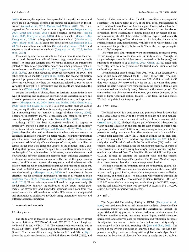
Sensitivity Analysis (SA) is a fundamental step in understanding theparameters influence on model behavior, and has role to decrease thenumber of parameters when calibration process is required (VanGriensven and Bauwens, 2003). In hydrological modeling the SA isdefined as a function that investigates the change in model outputsrelated to the changes in their parameters. The Global Sensitive Ana-lysis has the capacity to evaluate the influence of the parametersthroughout its range of variation, incorporating the uncertainty factorunder this variation (Song et al., 2015; Wang et al., 2013). The sensi-tivity may vary according to the approach used, thus, it is needed to usedifferent objective functions to activate an efficient model calibration.In this study the Global Sensitivity Analysis was apply to the SWATmodel, and helps to identify the most dominant parameters that shouldbe used for calibration (Table 1).

The sensitivity ranking is defined by the evaluation of two coeffi-cients: the t-stat index, obtained dividing the parameter coefficientfound in the multiple regression analysis by the standard error; and thep-value hypothesis test (Student’s test). The t-stat index is a better choicefor the modeler to understand the magnitude of the sensibility, whilethe p-value is better to define which parameters are more sensitive; weuse the p-value to define the most sensitive parameters. A low p-value(≤0.05) indicates that the null hypothesis can be rejected, the predictorthat has low value is likely to be a meaningful addition to the model,because changes in the predictor’s value are related to changes in the

response variable. With a p-value of 0.05, there is only a 5% chance thatresults would have come up in a random distribution, with a 95%probability of being correct that the variable is having some effect inthe output (Abbaspour et al., 2004; Me et al., 2015).

Table 1 describes all parameters obtained in SA for the two cali-bration methods. The check mark indicates that model was sensitive tothe parameter for that calibration method and that the parameter wasused in the calibration process. The selected parameters belong to themodel routines of groundwater, management, main channel, HRU’s,basin physical process, soil, and plant growth. The range column in-dicates the initial parameter distribution during the sensitive analysisand the calibration process, the values are based on the available in-formation and physical meaning., The methods used to adjust theparameters values in SUFI-2 are represented as the first letter before theparameters name (R, V, and A); the letter V represents replacing theexisting parameter value, A is adding a given value to the existingparameter value, and R is multiplying (1+ a given value) to the ex-isting parameter value. The last column indicates if the main parameterinfluence is related to streamflow or suspended sediment processes.

The SA was done for the two different calibration methods, se-quential and simultaneous, and for the two objective functions, NS andKGE. In sequential calibration, the sensitivity was made first for thestreamflow parameters, and after for the suspended sediment para-meters. In simultaneous calibration, all parameters were modified to-gether in the analysis. In relation to the objective functions, two para-meters sets were obtained, one for NS and one for KGE. The GlobalSensitivity Analysis was carried out using SUFI-2 and 1 iteration with2000 runs was made to activate the sensitive parameters. The initialparameters were all the listed in the model manual, a total of 25 wereselected, where 20 were used in the sequential calibration and 17 in thesimultaneous one. Related to the process influence, 17 are for stream-flow influence, and 8 are for suspended sediment

Fig. 1. Study area location in Santa Catarina state, southern Brazil.

T.M. Brighenti et al. Ecological Engineering 127 (2019) 103–113

105

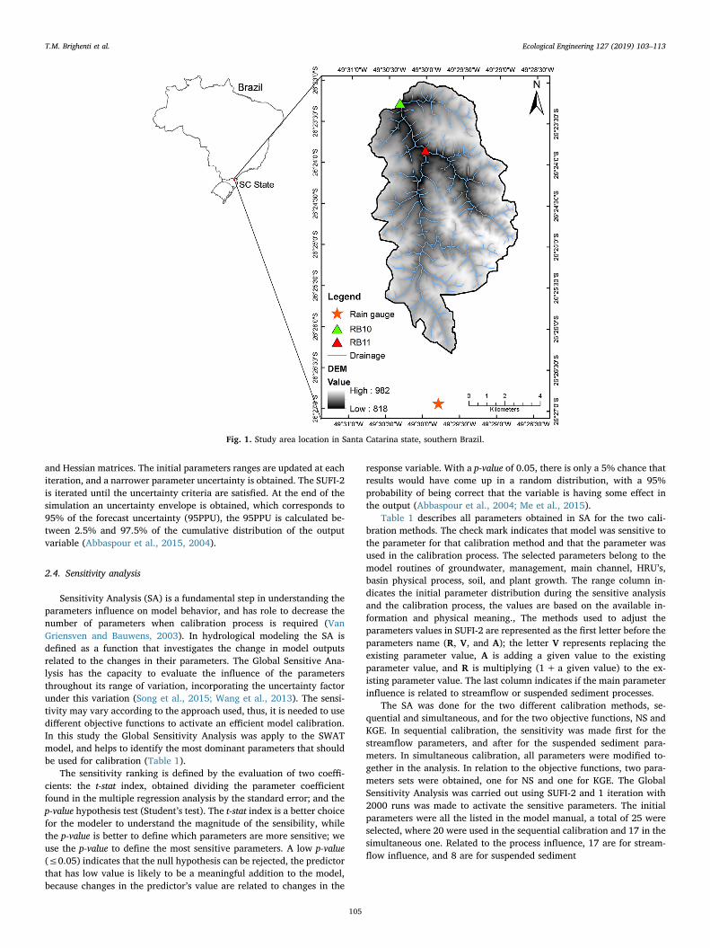
2.5. Calibration process

Considering the objective of this study, the SWAT model was onlycalibrated, not validated and the SUFI-2 algorithm was used. The pro-cedure requires objective functions, which will optimize the search inthe parameter space and find the best combinations that reflect thewatershed and data characteristics (Sun et al., 2017). The uncertaintyanalysis is a consequence of calibration process and will deal with theequifinality phenomena. Fig. 2 illustrates the calibration process, thefollow approaches are: (i) the model run 2000 times, for 4 iterations;(ii) multi-variable, the parameters are calibrated on different observed

variables (e.g., streamflow and suspended sediment); (iii) multi-site, theparameters are calibrated against different sites (e.g., RB10 and RB11);and (iv) multi-objective, more than one objective function is used incalibration (Nash-Sutcliffe and King-Gupta Efficiency). All these pro-cedures are mixed with the two calibration methods.

The final model parameter ranges are always conditioned on theform of the objective function (Shrestha et al., 2016). Actually, thereare several objective functions in the literature, including statisticallybased and maximum likelihood (Oudin et al., 2006). In this study wefocus our choice in two purposes, a simple easy interpretation andhighly literature recommendation. Then, to activate the multi-objective

Table 1Parameter range and calibration used in the Sensitivity Analysis. The first letter before the parameters name indicates the adjusted method in SUFI-2. The check markindicates that the model is sensitive to the parameter for each calibration method. The process column indicates if the parameter is mainly related to streamflow orsuspended sediment.

Parameters Range Calibration Method Process

Max. Min. Simultaneous Sequential

A__GWQMN.gw −1000.00 1000.00 ✓ ✓ streamflowV__GW_REVAP.gw 0.020 0.20 ✓ ✓ streamflowA__RCHRG_DP.gw −0.05 0.05 ✓ streamflowA__GW_DELAY.gw −56.33 −8.45 ✓ streamflowR__CN2.mgt −0.10 0.10 ✓ ✓ streamflowR__CH_W2.rte −0.15 0.15 ✓ streamflowR__CH_S2.rte −0.15 0.15 ✓ ✓ streamflowV__CH_N2.rte 0.010 0.20 ✓ ✓ streamflowV__CH_K2.rte 0 10 ✓ ✓ streamflowR__CH_L2.rte −0.09 0.012 ✓ streamflowV__CH_COV1.rte 0 1 ✓ s. sedimentV__CH_COV2.rte 0 1 ✓ ✓ s. sedimentV__CH_BED_D50.rte 100 6000 ✓ ✓ s. sedimentV__LAT_TTIME.hru 0 100 ✓ streamflowV__ESCO.hru 0.7 0.95 ✓ streamflowR__SLSUBBSN.hru −0.2 0.2 ✓ ✓ s. sedimentR__OV_N.hru −0.29 −0.078 ✓ streamflowV__LAT_SED.hru 0 5000 ✓ ✓ s. sedimentV__SPCON.bsn 0.0001 0.01 ✓ ✓ s. sedimentV__SPEXP.bsn 1 1.5 ✓ ✓ s. sedimentV__SURLAG.,bsn 5.54 14 ✓ streamflowR__MSK_CO1.bsn −0.004 0.46 ✓ streamflowR__MSK_CO2.bsn −0.63 0.01 ✓ streamflowR__USLE_C{6}.plant.dat −0.2 0.2 ✓ s. sedimentR__USLE_C{7}.plant.dat −0.2 0.2 ✓ s. sedimentR__SOL_BD.sol −0.23 −0.07 ✓ streamflow

Fig. 2. Diagram of the calibration methods.

T.M. Brighenti et al. Ecological Engineering 127 (2019) 103–113

106

calibration method two objective function were chosen, the Nash-Sut-cliffe (NS) (Nash and Sutcliffe, 1970) and King-Gupta Efficiency (KGE)(Gupta et al., 2009). These two formulations were widely used andsuggested in SWAT and hydrological model application (e.g., Schaefliand Gupta, 2007; Asadzadeh et al., 2016; Guse et al., 2017; Kayasthaet al., 2013; Nicolle et al., 2014; Magand et al., 2015; Osuch et al.,2015). When a single indicator is used may lead to incorrect verificationof the model. Instead, a combination of graphical results, absolute valueerror, and normalized goodness-of-fit statistics is currently re-commended (Ritter and Muñoz-Carpena, 2013). Therefore, togetherwith the statistical indexes (NS, KGE, Pbias, p-factor, r-factor, r2), agraphical analysis (hydrographs, duration curves, histograms andscatter plots) were used to compare the simulated and observed data.

The NS is the most used objective function in hydrological modelingand in SWAT model application. It is a normalized statistic that de-termines the relative magnitude of the residual variance compared tothe measured data variance, its priority to high values of sampling is acommon point discussed by various authors (Asadzadeh et al., 2016;Guse et al., 2017; Moriasi et al., 2007; Schaefli and Gupta, 2007). TheNS values range between -∞ to 1, where 1 is a perfect simulation, zerorepresenting balance accuracy, and observations below zero representunacceptable model performance. According to Moriasi et al. (2007)the NS values≥ 0.5 were considered satisfactory model performancefor flow and sediment.

= − ⎡

⎣⎢

∑ −∑ −

⎤

⎦⎥

=

=

NSX X

X X1

( )( )

in

iobs

isim

in

iobs mean

12

12

where Xisim is simulated values; Xi

obs is observed values; X mean is themean of n observed values.

The KGE is the decomposition of NS in three components (alpha,beta and r), which can be separately considered at each iteration, ifnecessary. The formulation also allows for unequal weighting of thethree components if one wishes to emphasize certain areas of the ag-gregate function tradeoff space. The KGE ranges from −∞ to 1, aperformance above 0.75 and 0.5 is considered to be as good and in-termediate, respectively. The ideal coefficient value is one.

= − − + − + −KGE r α β1 ( 1) ( 1) ( 1)2 2 2

where r is the correlation coefficient between observed and simulatedvalues; α is the measure of relative variability in the simulated andobserved values; and β is the bias normalized by the standard deviationin the observed values.

The model performance was evaluated using four well-known sta-tistical criteria: NS; KGE; Percent bias (Pbias) (Gupta et al., 1999); p-factor and r-factor (Abbaspour et al., 2004). The NS and KGE coeffi-cients were used in the SUFI-2 algorithm in calibration process; thePbias, r-factor and p-factor statistical indexes were used only for modelevaluation after calibration. They were chosen because assess differentmodeling skills. The Pbias evaluates the trend that the average of thesimulated values has in relation to the observed ones. The ideal value ofPbias is zero (%); a good model performance could be±25% forstreamflow and±55% for suspended sediment, positive values in-dicate a model underestimation and negative values overestimation.

= ⎡

⎣⎢

∑ −∑

⎤

⎦⎥ ∗=

=

PbiasX X

X( )

( )100i

niobs

isim

in

iobs

12

1

where Xisim is simulated values; and Xi

obs is observed values.The p-factor and r-factor are the two uncertainty measured offered

by SUFI-2. The p-factor is the percentage of observed data bracketed bythe 95PPU. The r-factor is equal to the average thickness of 95PPU banddivided by the standard deviation of the observed data. A p-factor of oneand r-factor of zero is a simulation that exactly matches the observeddata. However, p-factor above of 0,70 and a r-factor under of 1,5 can beconsidered satisfactory simulations (Abbaspour et al., 2015).

=p factor nXn

- in

=∑ −=r factor

X X

σ-

( )n tn

tM

tM

obs

11i i i,97.5% ,2.5%

where XtMi,97.5% and Xt

Mi,2.5% represent the upper and lower simulated

boundaries at the time ti of the 95PPU; n is the number of observed datapoints; M refers to modeled; ti is the simulation time step; σobs stands forthe standard deviation of the measured data; and nXin is the number ofobserved data in the 95PPU interval.

2.6. Uncertainty analysis of observed data

To incorporate the measured data errors in uncertainty analysis, theTopping (1972)formulation was used. The formulation is widely ac-cepted (Bonumá et al., 2013; Harmel et al., 2006; Rodrigues et al.,2015). The error value for each measured data is provided by Harmelet al. (2006) and the best scenarios were chosen. Uncertainty infers instreamflow and suspended sediment measured values was based on thefollowing methods: velocity-area method, stage-discharge relationship,and automated sampling. These values are incorporated in SUFI-2 si-mulations and used to calculate the p-factor.

∑= ⎡

⎣⎢

⎤

⎦⎥

=

En

d1 ( )ps

n

s1

2

12

where Ep is the probable error range (±%); n is the number of po-tential errors sources; and ds

2 are the uncertainties associated with eachpotential error source.

3. Results and discussion

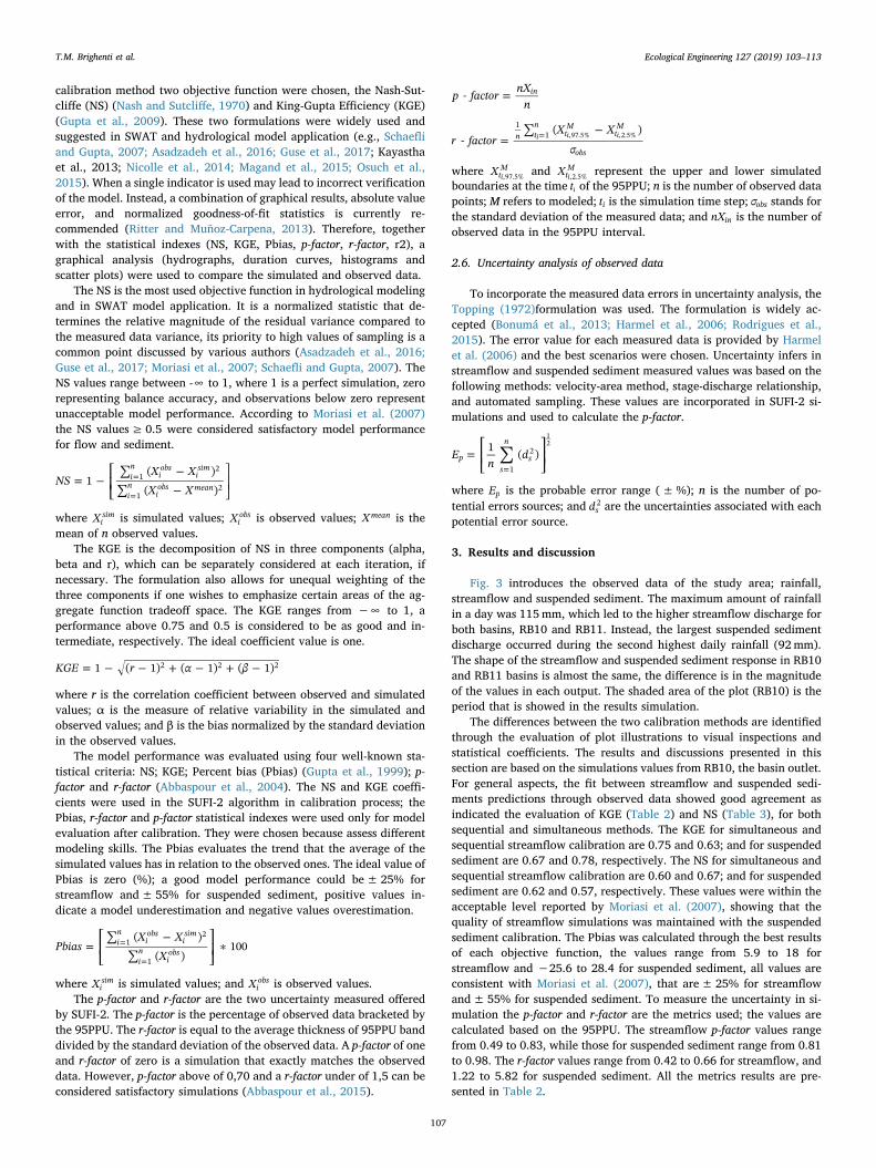
Fig. 3 introduces the observed data of the study area; rainfall,streamflow and suspended sediment. The maximum amount of rainfallin a day was 115mm, which led to the higher streamflow discharge forboth basins, RB10 and RB11. Instead, the largest suspended sedimentdischarge occurred during the second highest daily rainfall (92mm).The shape of the streamflow and suspended sediment response in RB10and RB11 basins is almost the same, the difference is in the magnitudeof the values in each output. The shaded area of the plot (RB10) is theperiod that is showed in the results simulation.

The differences between the two calibration methods are identifiedthrough the evaluation of plot illustrations to visual inspections andstatistical coefficients. The results and discussions presented in thissection are based on the simulations values from RB10, the basin outlet.For general aspects, the fit between streamflow and suspended sedi-ments predictions through observed data showed good agreement asindicated the evaluation of KGE (Table 2) and NS (Table 3), for bothsequential and simultaneous methods. The KGE for simultaneous andsequential streamflow calibration are 0.75 and 0.63; and for suspendedsediment are 0.67 and 0.78, respectively. The NS for simultaneous andsequential streamflow calibration are 0.60 and 0.67; and for suspendedsediment are 0.62 and 0.57, respectively. These values were within theacceptable level reported by Moriasi et al. (2007), showing that thequality of streamflow simulations was maintained with the suspendedsediment calibration. The Pbias was calculated through the best resultsof each objective function, the values range from 5.9 to 18 forstreamflow and −25.6 to 28.4 for suspended sediment, all values areconsistent with Moriasi et al. (2007), that are± 25% for streamflowand± 55% for suspended sediment. To measure the uncertainty in si-mulation the p-factor and r-factor are the metrics used; the values arecalculated based on the 95PPU. The streamflow p-factor values rangefrom 0.49 to 0.83, while those for suspended sediment range from 0.81to 0.98. The r-factor values range from 0.42 to 0.66 for streamflow, and1.22 to 5.82 for suspended sediment. All the metrics results are pre-sented in Table 2.

T.M. Brighenti et al. Ecological Engineering 127 (2019) 103–113

107

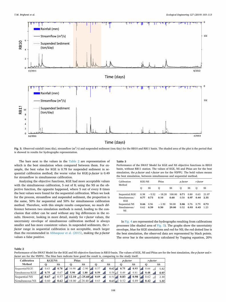
The bars next to the values in the Table 2 are representation ofwhich is the best simulation when compared between them. For ex-ample, the best value for KGE is 0.78 for suspended sediment in se-quential calibration method; the worse value for KGE/p-factor is 0.49for streamflow in simultaneous calibration.

Analyzing the objective functions, KGE had more acceptable valueswith the simultaneous calibration, 5 out of 8; using the NS as the ob-jective function, the opposite happened, where 5 out of every 8 timesthe best values were found for the sequential calibration. When we lookfor the process, streamflow and suspended sediment, the proportion isthe same, 50% for sequential and 50% for simultaneous calibrationmethod. Therefore, with this simple results comparison, no much dif-ference between two simulation methods is noted, leading to the con-clusion that either can be used without any big differences in the re-sults. However, looking in more detail, mainly for r-factor values, theuncertainty envelope of simultaneous calibration method is alwayssmaller and has more consistent values. In suspended sediments, the r-factor range in sequential calibration is not acceptable, much largerthan the recommended in Abbaspour et al. (2015), making the p-factorvalues a false positive.

In Fig. 4 are represented the hydrographs resulting from calibrationsprocesses (the shaded area of Fig. 3). The graphs show the uncertaintyenvelope, blue for KGE simulations and red for NS; the red dotted line isthe best simulation, the observed data are represented by black points.The error bar is the uncertainty calculated by Topping equation, 20%

Fig. 3. Observed rainfall (mm/dia), streamflow (m3/s) and suspended sediment (ton/day) for the RB10 and RB11 basin. The shaded area of the plot is the period thatis showed in results for hydrographs representation.

Table 2Performance of the SWAT Model for the KGE and NS objective functions in RB10 basin. The values of KGE, NS and Pbias are for the best simulation, the p-factor and r-factor are for the 95PPU. The blue bars indicate how good the result is, comparing to the study itself.

Table 3Performance of the SWAT Model for KGE and NS objective functions in RB10basin, without RB11 station. The values of KGE, NS and Pbias are for the bestsimulation, the p-factor and r-factor are for the 95PPU. The bold values meansthe best simulation, between simultaneous and sequential method.

CalibrationMethod

KGE/NS Pbias p-factor r-factor

Q SS Q SS Q SS Q SS

Sequential/KGE 0.38 −5.52 −18.20 100.00 0.71 0.80 0.63 21.07Simultaneous/

KGE0.77 0.73 0.10 0.60 0.50 0.97 0.44 2.35

Sequential/NS 0.66 0.56 −1.50 50.00 0.86 0.76 0.79 0.73Simultaneous/

NS0.62 0.59 0.50 29.00 0.52 0.93 0.43 1.23

T.M. Brighenti et al. Ecological Engineering 127 (2019) 103–113

108

for streamflow and 33% for suspended sediment. The duration curvescalculated with the entire time series data used in the process are shownat the top right corner of the hydrographs. The comparisons for theobserved and model simulated streamflow show an overall goodagreement in basin patterns with some discrepancies in low values, forboth sequential and simultaneous calibration. The best duration curvefit is in KGE simultaneous calibration, but the smaller uncertainty rangeis in NS sequential calibration. In suspended sediment the best curveduration fit and the smaller uncertainty range are in simultaneous ca-libration, even with the NS calibration having more than 50% of thesimulation values equal to zero. None of the model configurations wasable to capture the suspended sediment low values, which might beattributed to the very small values of observed data. We raised twohypotheses, which should be investigated in future, for this fact. One, isthe use of Bagnold equation. According to Wu and Chen (2012), Bag-nold method behaves better for simulating high sediment concentrationin high flows. The other is regarding the simulation time step, daily

basis, which can be insufficient to capture the basin behavior duringlow suspended sediment discharge. The histograms and the scatter plotsof observed data and the best simulation are shown in Fig. 5.

The frequency distribution that best fits with the streamflow ob-served data is in the KGE simultaneous calibration results, for sus-pended sediments the NS simultaneous distribution show more con-sistency. The highest histograms heights are always corresponding,showing a positive association between the two variables. In the scatterplot analysis the strongest relationship for streamflow is in NS se-quential calibration, for suspended sediments in NS simultaneous cali-bration. An improvement by simultaneous calibration is also noted inthe values magnitude of the simulated peaks (see Fig. 4). The sequentialcalibration, for example, simulates a suspended sediment yield of ap-proximately 80 ton/day, for KGE objective function, when the max-imum observed value on this day was approximately 6 tons/day. Si-multaneous calibration also presents high simulated values for thisevent, but the values do not exceed 15 ton/day.

Fig. 4. Hydrographs results representation for calibrations processes (the shaded area of Fig. 3). The graphs show the uncertainty envelope (95PPU), the blue is forKGE objective function simulations and the red is for NS; the red dotted line is the best simulation result, the observed data is represented by the black points. Theerror bar is the uncertainty calculated by Topping equation, 20% for streamflow and 33% for suspended sediment. The duration curves are shown at the top rightcorner of the hydrographs and were calculated with the entire time series data used in the calibration process. (For interpretation of the references to colour in thisfigure legend, the reader is referred to the web version of this article.)

T.M. Brighenti et al. Ecological Engineering 127 (2019) 103–113

109

Fig. 6 demonstrates the objective functions values for the 2000 si-mulations of the last model iteration. The red line is the threshold forthe behavioral solutions, we choose the limit of 0.5 for streamflow andsuspended sediment, for both objective functions. The dots above the

line are behavioral solutions with the best parameters estimation. Forthe two methods, the majority of streamflow simulation are above limit.For suspended sediment, the numbers of behavioral solutions are dif-ferent from one method to another, the method that presents the

Fig. 5. Relationship between the observed and simulated data for streamflow and suspend sediment. On the right, the histograms with the frequency distributions; onthe left, the respective scatter plot with the reference lines.

T.M. Brighenti et al. Ecological Engineering 127 (2019) 103–113

110

greatest amount of acceptable results is the KGE simultaneous methodwith, 38% of behavioral solutions.

In an attempt to validate the conclusions, we made a small mod-ification in the RB10 basin calibration process. The modification con-sists in a calibration process simplification, where the RB11 station wasremoved of the process, meaning that multi-site calibration no longerexists. Summarizing, the patterns are same, and the simultaneous ca-libration has more satisfactory results. 7 of 8 for NS objective functionand 5 of 8 for KGE (Table 3). We also found that multi-site calibrationtechnique improves the results in 3 out of every 4 simulations for sus-pended sediments, indicating the importance of including multiplemonitoring points in SS model calibration. For streamflow, the im-provement was not significant, while both the sequential and the si-multaneous simulations using NS were similar; one had better resultsusing the KGE sequential rather that with the KGE simultaneous si-mulation (Tables 2 and 3).

Furthermore, the simultaneous calibration is less time consuming;in sequential we have a total of 7 iterations (3 for streamflow and 4 forsuspended sediment), counts 4 iterations of the simultaneous calibra-tion. The number of parameters required in the simultaneous calibra-tion process is also smaller, which according to Daggupati et al. (2015)and Finger et al. (2012) reduces the equifinality problems, since it isexpected that fewer model parameters sets can satisfy the calibrationcriteria. That might indicate which field data are more important to bemonitored in order to improve calibration and the understanding of thedominant streamflow generation processes in the basin.

4. Conclusions

This study investigated the impact of sequential and simultaneouscalibration methods for streamflow (Q) and suspended sediment (SS)simulations using the SWAT. We have analyzed the differences betweenthe two methods through statistical indexes and graphical representa-tion.

We found that it is important to analyze a combination of statisticalindexes and graphical solutions, to reduce the subjectivity commonlyintroduced by only one evaluation approach. More specifically, whenKGE was used as objective function the results were more acceptable insimultaneous calibration, for NS the best values were in sequentialcalibration. The quality of streamflow simulation was maintainedduring the suspended sediment calibration.

In the hydrographs and the flow duration curve analyses we noticedthat while the model simulations for baseflow conditions were less sa-tisfactory, there was a general good fit for medium and high values. Thetotal uncertainty range was smaller in simultaneous calibration, forboth streamflow (Q) and suspended sediments (SS). In the frequencydistribution, the highest histograms heights are always corresponding,showing a positive association between the simulated and observedvalues. Regarding to the behavioral solution in the calibration methodsthe majority of streamflow simulations are above limit. For suspendedsediment, the numbers of behavioral solutions are different from onemethod to another; the method that presents the greatest amount ofacceptable results is the KGE simultaneous method, with 38% of be-havioral solutions. Therefore, the simultaneous calibration presentedadvantages in relation to the sequential.

Additionally, we also found that multi-site calibration method im-proves the results in 3 of 4 simulations for suspended sediments, in-dicating the importance of including multiple monitoring points in SSmodel calibration.

Since our analysis has been made for a small basin with two mon-itoring points, it is important that the study be extended to larger basinswith more monitoring points. Also, the use of a multi-objective ap-proach (e.g., Oudin et al., 2006) an alternative to hydrological modelcalibration. Finally, the use of sub-daily data with a different SSequation is also recommended, in order to correct the low values si-mulation problems.

Acknowledgements

The authors would like to thank the Associate Editor and the twoanonymous reviewers whose suggestions greatly improved the manu-script; the CNPq (National Council for Scientific and TechnologicalDevelopment) and PPGEA-UFSC (Environmental Engineering Pos-Graduation Program of Federal University of Santa Catarina) for a PhDfinancial support; and to Hydrology Laboratory team-UFSC for thesupport during the research time.

References

Abbaspour, K.C., Faramarzi, M., Ghasemi, S.S., Yang, H., 2009. Assessing the impact ofclimate change on water resources in Iran. Water Resour. Res. 45, 1–16. https://doi.org/10.1029/2008WR007615.

Fig. 6. The behavioral simulation representation n. The black dots are the objective functions values for the 2000 simulations of the last model iteration. The red lineis the threshold for the behavioral solution. The limit is: 0.5 for streamflow and suspended sediment, for both objective functions. (For interpretation of the referencesto colour in this figure legend, the reader is referred to the web version of this article.)

T.M. Brighenti et al. Ecological Engineering 127 (2019) 103–113

111

Abbaspour, K.C., Johnson, C.A., van Genuchten, M.T., 2004. Estimating uncertain flowand transport parameters using a sequential uncertainty fitting procedure. Vadose Zo.J. 3, 1340. https://doi.org/10.2136/vzj2004.1340.

Abbaspour, K.C., Rouholahnejad, E., Vaghefi, S., Srinivasan, R., Yang, H., Kløve, B., 2015.A continental-scale hydrology and water quality model for Europe: calibration anduncertainty of a high-resolution large-scale SWAT model. J. Hydrol. 524, 733–752.https://doi.org/10.1016/j.jhydrol.2015.03.027.

Abeyou, W.W., Ayana, E.K., Yen, H., Jeong, J., MacAlister, C., Taylor, R., Gerik, T.J.,Steenhuis, T.S., 2018. Evaluating hydrologic responses to soil characteristics usingSWAT model in a paired-watersheds in the Upper Blue Nile Basin. Catena 163,332–341. https://doi.org/10.1016/j.catena.2017.12.040.

Andreassian, V., Perrin, C., Berthet, L., Moine, N Le, Lerat, J., Loumagne, C., Oudin, L.,Mathevet, T., Ramos, M.-H., Valery, A., 2009. HESS Opinions “Crash tests for astandardized evaluation of hydrological models”. Earth 1757–1764.

Arnold, J.G., Moriasi, D.N., Gassman, P.W., Abbaspour, K.C., White, M.J., Srinivasan, R.,Santhi, C., Harmel, R.D., Griensven, A Van, VanLiew, M.W., Kannan, N., Jha, M.K.,2012. Swat: model use, calibration, and validation. ASABE 55, 1491–1508.

Arnold, J.G., Youssef, M.A., Yen, H., White, M.J., Sheshukov, A.Y., Sadeghi, A.M.,Moriasi, D.N., Steiner, J.L., Amatya, D.M., Skaggs, R.W., Haney, E.B., Jeong, J.,Arabi, M., Gowda, P.H., 2015. Hydrological processes and model representation:impact of soft data on calibration. Trans. ASABE 58, 1637–1660. https://doi.org/10.13031/trans.58.10726.

Asadzadeh, M., Leon, L., Yang, W., Bosch, D., 2016. One-day offset in daily hydrologicmodeling: an exploration of the issue in automatic model calibration. J. Hydrol. 534,164–177. https://doi.org/10.1016/j.jhydrol.2015.12.056.

Beven, K., 2006. A manifesto for the equifinality thesis. J. Hydrol. 320, 18–36. https://doi.org/10.1016/j.jhydrol.2005.07.007.

Beven, K., Binley, A., 1992. The future of distributed models: model calibration anduncertainty preditiction. Hydrol. Process. 6, 279–298.

Beven, K., Smith, P.J., Wood, A., 2011. On the colour and spin of epistemic error (andwhat we might do about it). Hydrol. Earth Syst. Sci. 15, 3123–3133. https://doi.org/10.5194/hess-15-3123-2011.

Bonumá, N.B., Rossi, C.G., Arnold, J.G., Reichert, J.M., Paiva, E.M.C.D., 2013. Hydrologyevaluation of the soil and water assessment tool considering measurement un-certainty for a small watershed in Southern Brazil. Appl. Eng. Agric. 29, 189–200.https://doi.org/10.13031/2013.42651.

Cardoso, A.T., 2013. Estudo Hidrossedimentológico em Três Bacias Embutidas noMunicípio de Rio Negrinho – SC.

Daggupati, P., Pai, N., Ale, S., Douglas-Mankin, K.R., Zeckoski, R.W., Jeong, J., Parajuli,P.B., Saraswat, D., Youssef, M.A., 2015. A recommended calibration and validationstrategy for hydrologic and water quality models. Trans. ASABE 58, 1705–1719.https://doi.org/10.13031/trans.58.10712.

Fenicia, F., Savenije, H.H.G., Matgen, P., Pfister, L., 2006. Is the groundwater reservoirlinear? Learning from data in hydrological modelling. Hydrol. Earth Syst. Sci.Discuss. 10, 139–150. https://doi.org/10.5194/hessd-2-1717-2005.

Finger, D., Heinrich, G., Gobiet, A., Bauder, A., 2012. Projections of future water re-sources and their uncertainty in a glacierized catchment in the Swiss Alps and thesubsequent effects on hydropower production during the 21st century. Water Resour.Res. 48, 1–20. https://doi.org/10.1029/2011WR010733.

Folton, N., Andréassian, V., Duperray, R., 2015. Hydrological impact of forest-fire frompaired-catchment and rainfall–runoff modelling perspectives. Hydrol. Sci. J. 60,1213–1224. https://doi.org/10.1080/02626667.2015.1035274.

Gassman, P.W., Sadeghi, A.M., Srinivasan, R., 2014. Applications of the SWAT modelspecial section: overview and insights. J. Environ. Qual. 43, 1. https://doi.org/10.2134/jeq2013.11.0466.

Grison, F., 2013. Estudo da Geometria Hidráulica do Rio dos Bugres, do Município de RioNegrinho – SC.

Gupta, H.V., Sorooshian, S., Yapo, P.O., 1999. Status of automatic calibration for hy-drologic models: comparison with multilevel expert calibration. J. Hydrol. Eng.135–143. https://doi.org/10.1002/fut.20174.

Gupta, H.V., Sorooshian, S., Yapo, P.O., 1998. Toward improved calibration of hydrologicmodels: multiple and noncommensurable measures of information. Water Resour.Res. 34, 751–763. https://doi.org/10.1029/97WR03495.

Gupta, H.V., Kling, H., Yilmaz, K.K., Martinez, G.F., 2009. Decomposition of the meansquared error and NSE performance criteria: implications for improving hydrologicalmodelling. J. Hydrol. 377, 80–91. https://doi.org/10.1016/j.jhydrol.2009.08.003.

Guse, B., Pfannerstill, M., Gafurov, A., Kiesel, J., Lehr, C., Fohrer, N., 2017. Identifyingthe connective strength between model parameters and performance criteria. Hydrol.Earth Syst. Sci. Discuss. 1–30. https://doi.org/10.5194/hess-2017-28.

Harmel, R.D., Cooper, R.J., Slade, R.M., Haney, R.L., Arnold, J.G., 2006. Cumulativeuncertainty in measured streamflow and water quality data for small watersheds.ASABE 49, 689–701.

Hassan, M.A., Church, M., Yan, Y., Slaymaker, O., 2010. Spatial and temporal variation ofin – reach suspended sediment dynamics along the mainstem of Changjiang (YangtzeRiver), China. Water Resour. Res. 46, 1–14. https://doi.org/10.1029/2010WR009228.

Kirchner, J.W., 2006. Getting the right answers for the right reasons: linking measure-ments, analyses, and models to advance the science of hydrology. Water Resour. Res.42, 1–5. https://doi.org/10.1029/2005WR004362.

Klemeš, V., 1986. Operational testing of hydrological simulation models. Hydrol. Sci. J.31, 13–24. https://doi.org/10.1080/02626668609491024.

Krysanova, V., Srinivasan, R., 2015. Assessment of climate and land use change impactswith SWAT. Reg Environ. Chang. 15, 431–434. https://doi.org/10.1007/s10113-014-0742-5.

Magand, C., Ducharne, A., Le Moine, N., Brigode, P., 2015. Parameter transferabilityunder changing climate: case study with a land surface model in the Durance

watershed, France. Hydrol. Sci. J. 60, 1408–1423. https://doi.org/10.1080/02626667.2014.993643.

Me, W., Abell, J.M., Hamilton, D.P., 2015. Effects of hydrologic conditions on SWATmodel performance and parameter sensitivity for a small, mixed land use catchmentin New Zealand. Hydrol. Earth Syst. Sci. 19, 4127–4147. https://doi.org/10.5194/hess-19-4127-2015.

Moriasi, D., Wilson, B., 2012. Hydrologic and water quality models: use, calibration, andvalidation. Am. Soc. Agric. Biol. Eng. 55, 1241–1247. https://doi.org/10.13031/2013.42265.

Moriasi, D.N., Arnold, J.G., Van Liew, M.W., Binger, R.L., Harmel, R.D., Veith, T.L., 2007.Model evaluation guidelines for systematic quantification of accuracy in watershedsimulations. Trans. ASABE 50, 885–900. https://doi.org/10.13031/2013.23153.

Nash, J.E., Sutcliffe, J.V., 1970. River flow forecasting through conceptual models part I –a discussion of principles. J. Hydrol. 10, 282–290. https://doi.org/10.1016/0022-1694(70)90255-6.

Neitsch, S., Arnold, J., Kiniry, J., Williams, J., 2011. Soil & water assessment tool theo-retical documentation version 2009. Texas Water Resour. Inst. 1–647. https://doi.org/10.1016/j.scitotenv.2015.11.063.

Nicolle, P., Pushpalatha, R., Perrin, C., François, D., Thiéry, D., Mathevet, T., Le Lay, M.,Besson, F., Soubeyroux, J.M., Viel, C., Regimbeau, F., Andréassian, V., Maugis, P.,Augeard, B., Morice, E., 2014. Benchmarking hydrological models for low-flow si-mulation and forecasting on French catchments. Hydrol. Earth Syst. Sci. 18,2829–2857. https://doi.org/10.5194/hess-18-2829-2014.

Osuch, M., Romanowicz, R.J., Booij, M.J., 2015. The influence of parametric uncertaintyon the relationships between HBV model parameters and climatic characteristics.Hydrol. Sci. J. 60, 1299–1316. https://doi.org/10.1080/02626667.2014.967694.

Oudin, L., Andréassian, V., Mathevet, T., Perrin, C., Michel, C., 2006. Dynamic averagingof rainfall-runoff model simulations from complementary model parameterizations.Water Resour. Res. 42, 1–10. https://doi.org/10.1029/2005WR004636.

Ritter, A., Muñoz-Carpena, R., 2013. Performance evaluation of hydrological models:Statistical significance for reducing subjectivity in goodness-of-fit assessments. J.Hydrol. 480, 33–45. https://doi.org/10.1016/j.jhydrol.2012.12.004.

Rodrigues, D.B.B., Gupta, H.V., Mendiondo, E.M., Oliveira, P.T.S., 2015. Assessing un-certainties in surface water security: an empirical multimodel approach. WaterResour. Res. Res. 9013–9028. https://doi.org/10.1002/2014WR015432.Received.

Santhi, C., Arnold, J.G., Williams, J.R., Dugas, W.A., Srinivasan, R., Hauck, L.M., 2001.Validation of the SWAT model on a large river basin with point and nonpoint sources.J. Am. Water Resour. Assoc. 37, 1169–1188. https://doi.org/10.1111/j.1752-1688.2001.tb03630.x.

Santhi, C., Arnold, J.G., Williams, J.R., Dugas, W.A., Srinivasan, R., Hauck, L.M., 2002.Validation of the SWAT model on a large river basin with point and nonpoint sources.J. Am. Water Resour. Assoc. 37, 1169–1188. https://doi.org/10.1111/j.1752-1688.2001.tb03630.x.

Schaefli, B., Gupta, H.V., 2007. Do Nash values have value? Bettina. Hydrol. Process. 21,2075–2080. https://doi.org/10.1002/hyp.

Seibert, J., Mcdonnell, J.J., 2003. Calibration of Watershed models, sixth ed.Shrestha, B., Cochrane, T.A., Caruso, B.S., Arias, M.E., Piman, T., 2016. Uncertainty in

flow and sediment projections due to future climate scenarios for the 3S Rivers in theMekong Basin. J. Hydrol. 540, 1088–1104. https://doi.org/10.1016/j.jhydrol.2016.07.019.

Song, X., Zhang, J., Zhan, C., Xuan, Y., Ye, M., Xu, C., 2015. Global sensitivity analysis inhydrological modeling: review of concepts, methods, theoretical framework, andapplications. J. Hydrol. 523, 739–757. https://doi.org/10.1016/j.jhydrol.2015.02.013.

Sun, W., Wang, Y., Wang, G., Cui, X., Yu, J., Zuo, D., Xu, Z., 2017. Physically baseddistributed hydrological model calibration based on a short period of streamflowdata: Case studies in four Chinese basins. Hydrol. Earth Syst. Sci. 21, 251–265.https://doi.org/10.5194/hess-21-251-2017.

Surfleet, C.G., Tullos, D., 2013. Uncertainty in hydrologic modelling for estimating hy-drologic response due to climate change (Santiam River, Oregon). Hydrol. Process.27, 3560–3576. https://doi.org/10.1002/hyp.9485.

Thirel, G., Andréassian, V., Perrin, C., 2015. On the need to test hydrological modelsunder changing conditions. Hydrol. Sci. J. 60, 37–41. https://doi.org/10.1080/02626667.2015.1050027.

Topping, J., 1972. Errors of Observation and Their Treatment, fourth ed. Chapman andHall, London.

Van Griensven, A., Bauwens, W., 2003. Multiobjective autocalibration for semidistributedwater quality models. Water Resour. Res. 39, 1–9. https://doi.org/10.1029/2003WR002284.

Van Griensven, A., Ndomba, P., Yalew, S., Kilonzo, F., 2012. Critical review of SWATapplications in the upper Nile basin countries. Hydrol. Earth Syst. Sci. 16,3371–3381. https://doi.org/10.5194/hess-16-3371-2012.

Vandenberghe, V., Griensven, A. Van, Bauwens, W., Vanrolleghem, P.A., 2006. Effect ofdifferent river water quality model concepts used for river basin management deci-sions 277–284. https://doi.org/10.2166/wst.2006.322.

Vrugt, J., Beven, K., 2016. Embracing equifinality with efficiency: limits of acceptabilitysampling using the DREAM_ABC. J. Hydrol.

Wang, J., Li, X., Lu, L., Fang, F., 2013. Parameter sensitivity analysis of crop growthmodels based on the extended Fourier Amplitude Sensitivity Test method. Environ.Model. Softw. 48, 171–182. https://doi.org/10.1016/j.envsoft.2013.06.007.

Wellen, C., Arhonditsis, G.B., Long, T., Boyd, D., 2014. Quantifying the uncertainty ofnonpoint source attribution in distributed water quality models: a Bayesian assess-ment of SWAT’s sediment export predictions. J. Hydrol. 519, 3353–3368. https://doi.org/10.1016/j.jhydrol.2014.10.007.

Wu, H., Chen, B., 2015. Evaluating uncertainty estimates in distributed hydrologicalmodeling for the Wenjing River watershed in China by GLUE, SUFI-2, and ParaSol

T.M. Brighenti et al. Ecological Engineering 127 (2019) 103–113

112

methods. Ecol. Eng. 76, 110–121. https://doi.org/10.1016/j.ecoleng., 2014.05.014.Wu, Y., Chen, J., 2012. Science of the Total Environment Modeling of soil erosion and

sediment transport in the East River Basin in southern China. Sci. Total Environ. 441,159–168. https://doi.org/10.1016/j.scitotenv.2012.09.057.

Zeiger, S.J., Hubbart, J.A., 2016. Science of the Total Environment A SWAT model va-lidation of nested-scale contemporaneous stream flow, suspended sediment and nu-trients from a multiple-land-use watershed of the central USA. Sci. Total Environ.572, 232–243. https://doi.org/10.1016/j.scitotenv.2016.07.178.

Zhang, X., Srinivasan, R., Arnold, J., Izaurralde, R.C., Bosch, D., 2011. Simultaneouscalibration of surface flow and baseflow simulations: a revisit of the SWAT modelcalibration framework. Hydrol. Process. 25, 2313–2320. https://doi.org/10.1002/hyp.8058.

Zheng, F., Maier, H.R., Wu, W., Dandy, G.C., Gupta, H.V., Zhang, T., 2018. On lack ofrobustness in hydrological model development due to absence of guidelines for se-lecting calibration and evaluation data: demonstration for data-driven models. WaterResour. Res. 54, 1013–1030. https://doi.org/10.1002/2017WR021470.

T.M. Brighenti et al. Ecological Engineering 127 (2019) 103–113

113