Two Blades of the Scissors The Interaction between … 3.2 Knife-edge Growth: Aggregate 'Golden Age'...
36
1 Ronald Schettkat Oktober 2004 Two Blades of the Scissors The Interaction between Demand and Supply in Market Economies 3. Stable versus Knife-edge Growth, Potential and Actual Income Growth 3.1 Economic Growth: An Overview What are the major variables determining economic growth? Why do some countries experience very high rates of economic growth, while others have been stagnated, or even declined? Why do growth rates vary over time? Why did the Western capitalist countries experience such enormously high growth rates in the 1950s and 1960s, but comparatively low rates from the 1970s onwards? Ever since Adam Smith's 'Inquiry into the Wealth of Nations’ have issues of economic growth had a prominent place in economics. Views on the possibilities and limits of economic growth have varied from optimistic (Adam Smith) to pessimistic (Malthus and Ricardo). Today, there is still discussion about doom and boom scenarios. Some authors argue that productivity growth causes unemployment and predict ’the end of work’ (Rifkin 1996). Others see rising productivity rates as preconditions for a prosperous future (Bluestone/ Harrison 1999). It is also extensively discussed whether there is convergence or divergence between the leading economies and the ‘South’ (the developing countries). Scenarios of limited natural resources 1 , or ’limits of growth’, as published by the ’Club of Rome’ in 1972 (Meadows 1972) have also become popular in recent decades, and concerns about the environment, ‘global warming’, have gained importance and have 1 The economist Fred Hirsch (1976) has argued that there are social limits to growth. In his view, wellbeing significantly depends on positional goods, such as belonging to the top 10 %
-
Upload
truongkhue -
Category
Documents
-
view
214 -
download
0
Transcript of Two Blades of the Scissors The Interaction between … 3.2 Knife-edge Growth: Aggregate 'Golden Age'...

1
Ronald Schettkat Oktober 2004
Two Blades of the Scissors The Interaction between Demand and Supply in
Market Economies
3. Stable versus Knife-edge Growth, Potential and Actual Income Growth
3.1 Economic Growth: An Overview
What are the major variables determining economic growth? Why do some countries
experience very high rates of economic growth, while others have been stagnated, or
even declined? Why do growth rates vary over time? Why did the Western capitalist
countries experience such enormously high growth rates in the 1950s and 1960s, but
comparatively low rates from the 1970s onwards? Ever since Adam Smith's 'Inquiry
into the Wealth of Nations’ have issues of economic growth had a prominent place in
economics. Views on the possibilities and limits of economic growth have varied
from optimistic (Adam Smith) to pessimistic (Malthus and Ricardo). Today, there is
still discussion about doom and boom scenarios. Some authors argue that productivity
growth causes unemployment and predict ’the end of work’ (Rifkin 1996). Others see
rising productivity rates as preconditions for a prosperous future (Bluestone/ Harrison
1999). It is also extensively discussed whether there is convergence or divergence
between the leading economies and the ‘South’ (the developing countries). Scenarios
of limited natural resources1, or ’limits of growth’, as published by the ’Club of
Rome’ in 1972 (Meadows 1972) have also become popular in recent decades, and
concerns about the environment, ‘global warming’, have gained importance and have
1 The economist Fred Hirsch (1976) has argued that there are social limits to growth. In his view, wellbeing significantly depends on positional goods, such as belonging to the top 10 %

2
increasingly been discussed in connection to economic growth. Although these issues
are very important, here we will focus our discussion on the core economic issues of
growth, but other aspects will be touched on occasionally.
The perspective of theoretical work on economic growth has changed over time. In
the 1940s, the ‘Harrod-Domar model’ analyzed the full-employment stability
conditions of growth processes and predicted an unstable development of the
capitalist market economies. This prediction provoked Robert Solow (1956, 1987)
from MIT to design a ‘neoclassical growth model’ that allowed for factor
substitution, a mechanism used by Solow to show that the instability envisaged by
the Harrod-Domar model was due to the assumption of constant marginal
productivity of capital. Solow endogenized the relation between factors, that is, he
made the relative use of capital and labor dependent on their relative prices, and
assumed diminishing marginal productivity of individual factors. Thus, the Solow
model was built on stabilizing assumptions, which allowed a smooth and stable
growth path. By and large, Solow seems to right because the capitalist market
economies have turned out to be relatively stable in the long run, although they have
experienced marked ups and down in their economic growth, as discussed in the
previous chapter. Whether this long run stability is the result of self-correcting market
forces or caused by government interventions remains a subject of debate.
The Solow-Swan model (Swan 1956 had constructed a similar model independent
from Solow) has certainly become the most influential model of economic growth
among academics, and has determined the research agenda on growth theory. The
assumed diminishing returns to capital in the neoclassical growth model resulted in
the prediction that capital productivity is higher when the capital stock is small. In
other words, on the basis of this model, one would expect capital to flow from the
North (the industrialized world) to the South (the developing world), that is, from
countries with high capital stocks to countries with low capital stocks, thereby
stimulating high transitional growth rates in the South. If these predictions of the
neoclassical growth model would hold, incomes in the North and the South would
of wage earners. Positional goods are naturally limited, but economic growth creates the illusion that they are not.

3
eventually converge. We know, however, that this convergence has not occurred2,
and the lack of convergence has led to the creation of alternative growth models,
'endogenous growth theory’ or ‘new growth theory’, in which capital can show
constant or even increasing marginal productivity. Not only the old neoclassical
exogenous growth theory, but also the new endogenous growth theory emphasize the
supply side and neglect the role of demand. Evolutionary growth theory, in contrast,
recognizes the importance of both sides of the market, and regards growth as being
determined by the interaction between these two sides.
From today’s perspective, both traditional models of economic growth continue to be
relevant. The Harrod-Domar model is still pertinent because it has in common with
the new growth theory the possibility of constant marginal productivity of capital,
and because it incorporates the possibility of positive feedback effects, which is
arguably one force behind American productivity growth in the 1990s. The Solow
model is important because it continues to be the point of reference for many growth
studies, and even those economists who are skeptical about neoclassical growth
theory tend to refer to Solow who won the Nobel prize in 1987 for his work on
growth theory.
This chapter will briefly discuss the Harrod-Domar model of growth at the ’knife's
edge’, followed by a discussion of the exogenous neoclassical growth model (Solow-
Swan model), and will present estimates of the sources of growth, so-called growth
accounting. The issue of convergence will be discussed. In Chapter 4, new
endogenous growth theory will be examined, followed by a discussion of
evolutionary growth models in Chapter 5. This will link the theory of economic
growth to the subsequent investigations of unbalanced growth (Chapter 6), diffusion
processes, saturation and the microconditions for full employment as presented in
Chapters 7 to 10.
2 Although an important debate has been going on about the extent to which convergence has been brought about.

4
3.2 Knife-edge Growth: Aggregate 'Golden Age' Conditions (Harrod-Domar
Model)
The Harrod-Domar growth model (named after the British economist Roy Harrod
(Harrod, 1939 #288), and the American economist Evesey Domar (Domar, 1947
#289)) is not so much a model explaining the sources of economic growth, as a model
analyzing the conditions for equilibrium growth, that is, the conditions for a growth
path with full employment. It is a dynamic model, and an extension of the static
Keynesian model in which production adjusts in response to exogenous variations in
final demand (usually variations in investment) according to a multiplier process,
until income-dependent savings equal investments, and the economy has reached a
new equilibrium. The basic (static)3 Keynesian model comprises a self-correcting
mechanism or negative feedback effect, meaning that less investment leads to a
decline in income, and consequently in savings, until a new equilibrium has been
reached. If investment depends on expected changes in income and demand, an initial
decline in investment and income may result in lower subsequent investments and
hence income. In other words, from such a dynamic perspective, in which
investments are endogenous and driven by expectations, effects may be self-enforcing
rather than self-correcting. The dynamic model allows positive feedback to occur.
However, the Harrod-Domar model neglects the impact of relative prices on the
proportions of input factors, assuming that the capital-output ratio is constant (see
below). It is a one-sector growth model that follows in the footsteps of the Keynesian
revolution, in the sense that it is concerned with economic stability and
unemployment, and makes some rigid assumptions, which are not always useful in
long-run analyses. Its focus on expectation-driven investments makes the Harrod-
Domar model very applicable to recent trends in the US economy, whose boom of the
1990s was driven by (foreign) investment. Investment is directed at the future and
therefore always depends on expectations. However, economic theories differ with
3 In the static Keynesian model, production is determined by demand. A change in exogenous demand, such as investment in the Keynesian model, will change production according to the multiplier [m = I/ (I -C) = 1/s], where c is the marginal rate of consumption and s is the marginal rate of saving [c + s = 1].

5
respect to their explanations of investment decisions. Some refer to the ’animal spirit’
(Keynes 1936), implying that investment is driven by the ’feeling’ of entrepreneurs.
Others believe in ’rational expectations’ (Lucas/ Sargent 1978), implying that no
systematic mistakes are being made. (Stochastic perfect foresight, Arrow...)
Investment is a 'double-edged sword' (Domar, 1947 #289): it not only raises demand
(because investment is part of final demand) but also increases capacity. To keep
demand and supply in balance (in equilibrium), demand must grow with capacity, and
thus with investment. What is the rate of growth in investment needed to maintain full
employment? In other words, what is the rate of growth in investment that allows
capacity to grow exactly in line with demand? To achieve full employment, demand
and supply must grow in conjunction, planned investment and planned savings must
be equal and they must grow at the ‘warranted rate of growth’ (gw), which will be
explained shortly.4
The natural rate of growth is the sum of labor force growth (resulting either from a
growing population or from higher participation, see Chapter 2) and growth in labor
productivity, which can be thought of as technological progress in the Harrod-Domar
model. Since the productivity of capital is constant,5 technological progress is labor-
augmenting, meaning that it has the same output effect as using more labor, but is
neutral with respect to the productivity of capital. In other words, to produce a certain
output, the amount of capital needed stays the same and the capital-output ratio,
which is the inverse of capital productivity, remains constant.6 This specific
assumption on the effects of technological progress has become known as Harrod-
neutral technological change (see Box 3.3 on technological progress).
Because of the assumption that the capital-output ratio is constant, changes in
(expected) output must affect the amount of capital stock desired, and thus
4 Abstracting for variations in the components of final demand. 5 This assumption makes the Harrod-Domar model a member of so called ‘AK models’. A is an efficiency parameter (technology) and K is capital stock. 6 Capital productivity σ = Y / K, where Y is output and K is the capital stock. The capital-output ratio is the inverse of capital productivity, that is, K / Y.

6
investment. In a ‘naïve’7 investment function, this year’s investment (It) depends on
the need to replace depreciated capital stock, and on the expected change in output,
which in the simplest (naïve) version is equal to last year’s change in output (∆Yt-1).
∆K(desired) = I (desired) = α *∆Yt-1 + Kt-1 * δ (3.1)
where α = a constant and δ = the rate of depreciation
Substituting last year’s output change with expected output growth makes equation
3.1 more realistic:
∆ ∆K Y Kdesired t( ) * $ *= + −α δ1
where is the expected change in output (3.1a) ∆ $Y
To ensure full employment, production must grow in line with the labor force and
with the growth in (labor) productivity, which together constitute the so-called
'natural rate of growth’ (gn). This needs to be equal to the warranted rate of growth,
which is the growth rate at which savings and investments are in balance, and at
which capacity grows at exactly the same rate as demand. Full employment can only
be maintained if the economy grows on the path where ga = gw = gn.. It is purely
accidental when all three growth rates are identical, because there is no mechanism to
bring the natural rate of growth (gn) in line with the warranted rate of growth (gw) and
the actual rate of growth (ga). A situation in which all three growth rates are identical,
has been coined a 'Golden Age' by the British economist Joan Robinson, who thereby
indicated that a full-employment equilibrium is not only highly valuable, but also
extremely unlikely. Joan Robinson's idea of a 'Golden Age' abstracts, of course, from
changes in the structure of an economy and from the adjustment processes (both in
labor and other markets) needed to accommodate the aggregate rate of growth
7 ‘Naïve’ because interest rates, time lags between investment and available capacity and expected output changes are not taken into account.

7
Box 3.1: The Harrod-Domar Growth Model Harrod (1939) and Domar (1947) analyzed the aggregate conditions for a stable growth path with full employment. Three growth rates are important in their model: Natural Rate of Growth (gn) or Full-Employment Condition Full employment of labor is achieved if the economy grows at the natural rate of growth (gn), which is the sum of growth in the labor force (gL) and growth in labor productivity (gπ). This is also called labor-augmenting technological progress or Harrod-neutral technological progress (see Box 3.3 on technological progress). ∆Yn / Y = gn = gπ + gL (1) Warranted Rate of Growth (gw) By how much should investment increase to maintain a balanced growth path? According to the Keynesian multiplier, demand growth induced by additional investment is: ∆Yd = ∆I * m ; (2) where m = 1/ (1-c) = 1/s, c is the marginal rate of consumption from the Keynesian consumption function and s is the marginal savings rate (c + s = 1). Supply grows with net investment (investment minus depreciation), which is the change in capital stock (∆K) times capital productivity σ (σ = Y / K), and is assumed to be constant. ∆Ys = ∆K * σ = I * σ (3) At the equilibrium growth path, ∆Yd must be equal to ∆Ys , that is supply must grow in line with demand: ∆I * 1 / s = I * σ or ∆I / I = s * σ = S / Y * ∆Y / I (4) In equilibrium S = I (savings equal investment) and (4) is equal to the growth rate of output ∆Yw / Y, which has been labeled the warranted rate of growth (gw). That is the growth rate at which planned investment and planned savings are equal. In other words, at this rate of growth, the economy produces as many consumption goods as wanted by consumers and as many capital goods as wanted by producers. It is a dynamic equilibrium (or steady- state growth).
8
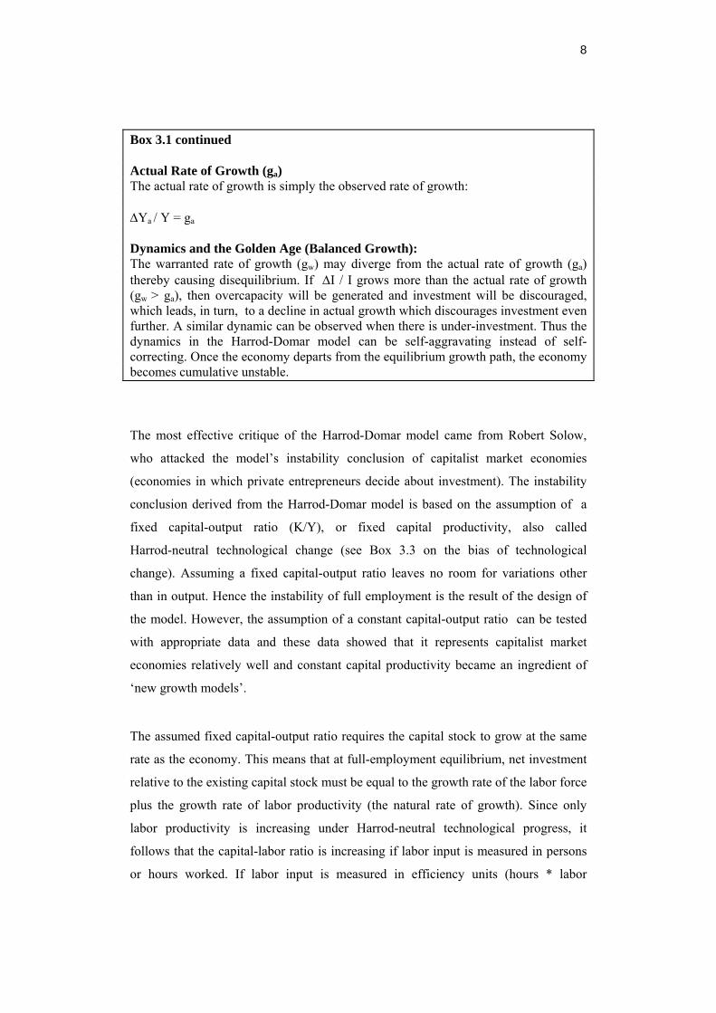
Box 3.1 continued Actual Rate of Growth (ga) The actual rate of growth is simply the observed rate of growth: ∆Ya / Y = ga Dynamics and the Golden Age (Balanced Growth): The warranted rate of growth (gw) may diverge from the actual rate of growth (ga) thereby causing disequilibrium. If ∆I / I grows more than the actual rate of growth (gw > ga), then overcapacity will be generated and investment will be discouraged, which leads, in turn, to a decline in actual growth which discourages investment even further. A similar dynamic can be observed when there is under-investment. Thus the dynamics in the Harrod-Domar model can be self-aggravating instead of self-correcting. Once the economy departs from the equilibrium growth path, the economy becomes cumulative unstable.
The most effective critique of the Harrod-Domar model came from Robert Solow,
who attacked the model’s instability conclusion of capitalist market economies
(economies in which private entrepreneurs decide about investment). The instability
conclusion derived from the Harrod-Domar model is based on the assumption of a
fixed capital-output ratio (K/Y), or fixed capital productivity, also called
Harrod-neutral technological change (see Box 3.3 on the bias of technological
change). Assuming a fixed capital-output ratio leaves no room for variations other
than in output. Hence the instability of full employment is the result of the design of
the model. However, the assumption of a constant capital-output ratio can be tested
with appropriate data and these data showed that it represents capitalist market
economies relatively well and constant capital productivity became an ingredient of
‘new growth models’.
The assumed fixed capital-output ratio requires the capital stock to grow at the same
rate as the economy. This means that at full-employment equilibrium, net investment
relative to the existing capital stock must be equal to the growth rate of the labor force
plus the growth rate of labor productivity (the natural rate of growth). Since only
labor productivity is increasing under Harrod-neutral technological progress, it
follows that the capital-labor ratio is increasing if labor input is measured in persons
or hours worked. If labor input is measured in efficiency units (hours * labor

9
productivity) the ratio of capital to efficiency units remains constant. Since prices
(wages) are not included in the Harrod-Domar model, the factor proportions used in
the production process are determined technologically and therefore do not depend on
relative factor prices. The elasticity of substitution between capital and labor is
assumed to be zero (see Box 3.4 on the elasticity of substitution). Since capital cannot
substitute labor, and relative factor prices are consequently unimportant, Robert
Solow developed the neoclassical growth model in which the use of production
factors is dependent on their marginal productivity.
Other criticisms of the Harrod-Domar model are that:
• Consumption and saving are taken from the simple Keynesian consumption
function and thus depend only on income. However, as will be discussed in
Chapter 7, consumption can also be influenced by a number of other
variables;
• The model is an aggregate model, which focuses on quantities and neglects
qualities such as new products, skills etc. Thereby it abstracts from product
and labor market frictions. This shortcoming is not unique to the
Harrod-Domar model, but applies equally to many other models, including
the neoclassical growth model;
• The idea of Harrod-neutral technological progress is incorrect;
• The measurement of capital is tricky;
• The assumption of exogenous technological progress (that is progress which
is not explained within the model), which is also made by the neoclassical
growth model, is problematic. Per capita income is driven by technological
progress, but it is not explained by the model (see also the section below on
the neoclassical growth model). It therefore does not explain economic
growth but merely explores the aggregate conditions for growth at full
employment.

10
Box 3.2: Balanced or Steady State Growth, Unbalanced Growth and ‘Golden Age’ Growth Balanced or Steady State Growth Balanced growth is a dynamic condition of an economy in which all real variables are growing at the same constant proportional rate. For example, each industry is growing at the same rate, thereby leaving the structure of the economy unchanged. Unbalanced Growth Unbalanced growth is a dynamic condition of an economy in which real variables are growing at different rates. For example, each industry is growing at a different rate, thereby changing the industry structure of the economy. ‘Golden Age’ Growth ‘Golden age’ growth is a situation of balanced growth in which the warranted rate of growth is equal to the natural rate of growth at full employment. The term was coined by Joan Robinson and reflects her view on the probability that such a state of affairs would arise in a capitalist economy without a government. In Robinson’s view, the concept of equilibrium is a 'thought experiment' designed to facilitate analysis (Robinson 1980). In equilibrium, expectations would never be falsified and whatever happened would be compatible with people’s expectations in each period of time. All expectations would continuously be fulfilled. The real world, however, is full of distortions and the ‘golden age’ condition: gn = gw = ga where the natural growth rate = the warranted growth rate = the growth rate of national income may not hold. Unless labor productivity would rise at a uniform rate across all sectors, and unless the real wage rate would also rise at this rate, technological progress would tend to distort the system of relative prices, as well as the distribution of income between wages and profit, which holds along any steady-state growth path.

11
Box 3.3: Bias in Technological Progress Technological change may be neutral, labor-saving, or capital- saving. It is common to draw a theoretical distinction between two different concepts of technological progress: Harrod-neutral and Hicks-neutral technological progress. According to Harrod (1948), technological progress is: • neutral if it leaves the capital-output ratio unchanged (that is capital productivity is constant); • labor-saving if it raises the capital-output ratio; • capital-saving if it lowers the capital-output ratio. The capital-output ratio or capital-coefficient (K/Y) is the inverse of capital productivity Y/K). Technological progress may reduce the need for, for example capital inputs in the production process, which in turn may lower the price of capital goods, and consequently increase the use of capital, thereby partly or totally offsetting the initial capital-saving effect. It may be misleading, therefore, to use the capital-output ratio as a measure for classifying technological progress if price reactions to changing factor demand are strong, and if the elasticity of substitution between factors is high. Hicks (1932) disentangled the effect of changes in the use of factors due to the pure technological effect from changes due to the price effect. According to Hicks, technological progress is: • neutral if it raises the marginal product of labor and capital proportionally, meaning that, if factor prices were held constant, the use of capital relative to labor would remain unchanged. In the figure below, technological progress shifts the production function from Y to Y' and the relative decline in K [(K-K')/K] equals the relative decline in L [(L-L') / L] needed to produce one unit of output (Y). • labor-saving if it raises the marginal product of capital more than the marginal product of labor, meaning that, if factor prices were held constant, less labor would be used. In the figure below, labor-saving technological progress shifts the production function from Y to Y", that is for given capital (K) less labor will be used (L") and L - L'' labor is being saved. • capital-saving if it raises the marginal product of labor more than the marginal product of capital, meaning that, if factor prices were held constant, less capital would be used. In the figure below, capital-saving technological progress shifts the production function from Y to Y''', that is for given labor (L) less capital will used (K"') and K-K''' capital is saved. Box 3.3: continued

12
Elasticity of Substitution The elasticity of substitution describes the shape of an isoquant (the Y-curves in the above figure) by the ratio of the relative change in factor proportions divided by the relative change in the slope of the isoquant. The latter is under the assumption of cost minimization equal to relative factor prices [d(K/L)/(K/L) = PL/PK] and the elasticity of substitution is:
σ =
FHGI FKJ HGIKJFHG
IKJ
d KL
KL
d PP
PP
L
K
L
K
That is, that say an elasticity of substitution of 0.1 indicates that an increase of the relative price of labor (relative to capital) of labor of 10% will change the relative factor proportions by 1%. Special values of the elasticity of substitution are 0, which means that changes in factor prices do not influence the factor proportions (so called Leontief production function in which the factor proportions are technically fixed, i.e. only one combination is cost minimizing). Another special value is 1, where changes in relative prices translate to proportional changes in factors used (Cobb-Douglas production function).

13
3.3 Stable Growth Patterns: Neoclassical Growth Solow-Swan Model
3.3.1 The Solow-Swan Model The most important model of economic growth, which during the last 50 years has
had a significant impact on research on economic growth, is the Solow-Swan model,
developed independently by the MIT economist and Nobel laureate Robert Solow and
Trevor Swan. Solow received the Nobel Prize for his work on economic growth, but
he has also made many other important contributions to economics. In his Nobel
lecture (Solow 1987) Solow expresses the dissatisfaction that he felt about the
instability conclusion derived from the Harrod-Domar model, which was based on the
assumption of constant capital productivity. He wanted to show that, if one relaxes
this assumption, capitalist economic development need not be unstable, and he
assumed decreasing marginal returns to capital (and labor) instead, meaning that he
assumed that marginal capital productivity declines.
Solow's starting point was an aggregate production function that combined capital
and labor in a similar way as the production function of an individual firm. In
microeconomic production theory, a firm is assumed to vary its factor inputs in
accordance with factor prices. In the optimal case, a firm will increase its use of labor
until the price of labor (the wage) equals its marginal (value) product. A similar rule
applies to capital. If factor prices change, the firm is presumed to adjust the amount of
capital and labor used, in order to equal prices to marginal productivity. This assumes
a flexible technology, which allows one factor of production to be substituted by
another8. In the neoclassical growth model, the aggregate economy is thought of as a
firm, meaning that the factor proportions used in production can be changed in order
to equal their price to their marginal value product. Under such conditions, full
employment can be achieved by varying factor inputs. If full employment has not yet
been realized, lower wages will stimulate the use of more labor (lower wages should
equal the marginal value product at higher employment) in the production process,
8 Actually, it is assumed that firms use different technologies if they change the proportions of capital and labor ({Foley, 1999 #18}).

14
thereby allowing for full employment. The shares of capital and labor that are used in
the production process will thus depend on relative factor prices9.
In the most basic function, output (Y) depends on the shares of capital (K) and labor
(L) used, where capital and labor each show diminishing returns or declining
marginal value products. That is, the elasticity of output with respect to variations in
one of the input factors is less than one.
Y F K L K L= =( , ) *α β (3.2)
Since the Solow model assumes market clearing, the elasticities (α and β) are the
shares of capital and labor in overall valued added, which are relatively stable in the
long run, with values of about α = 1/3 and β = 2/3. If α and β add up to one (β = 1 -
α), equation (3.2.) shows constant returns to scale, meaning that doubling the input of
capital and labor leads to a doubling of output10.
If function (3.2) is divided by labor (L), one gets production function the so-called
labor-intensive form:
YL
KL
=FHGIKJα
(3.3)
9 Solow (1956) concludes his paper with the qualification that his model is theoretical and therefore simplifying: ’Everything above is the neoclassical side of the coin. Most especially it is full employment economics –in the dual aspect of equilibrium conditions and frictionless, competitive, causal system’ (Solow 1956: 91). He also adds qualifications on wage rigidity, uncertainty etc. 10 0 < α <1, α + (1-β) = 1 constant returns to scale [f(aK, aL) = aY] f(aK, aL) > aY increasing returns to scale, f(aK, aL) < Y decreasing returns to scale

15
Figure 3.1: The Neoclassical Production Function
Y/L
K/L
In the neoclassical production function, the marginal returns to an increase of one
factor are diminishing. Figure 3.1 shows output per worker (Y/L = y) as a function of
capital per worker (K/L = k). The larger the amount of capital per worker, the higher
the output per worker (dy/dk > 0), although increases in output are diminishing with
every additional unit of capital (d2y/d2k < 0). Using more capital in the production
process can thus increase output per worker, but as the costs of capital (the interest)
increase, the value of the additional output may become less than the value of the
additional input, and an increase in capital becomes inefficient. In other words,
decreasing returns to factor inputs set efficiency limits to the use of specific factors,
thereby providing an equilibrium mechanism 11.
If capital is relatively more expensive than labor, the amount of capital used in the
production process will be smaller because the marginal product of capital (which is
higher when the capital stock is smaller) should equal the cost, and vice versa. This
may explain why capital-intensive production processes are dominant in the
]
]
11 In the Harrod-Domar model, the marginal productivity of capital is constant: [ / ; /dY dK d Y d K> =0 02 2
In the Solow-Swan model marginal productivity is diminishing: [ / ; /dY dK d Y d K> <0 02 2

16
industrialized world and labor-intensive production processes are dominant in
developing countries assuming hat production in the North and the South is subject to
the same production function (the same technology)12. Production in the South is less
capital intensive (left in Figure 3.1) because this is optimal for the South. In the
North, on the other hand, production is capital intensive (right in Figure 3.1) because
labor is relatively scarce and capital is relatively abundant. In this model, the use of
factor inputs is economically determined, rather than technologically. Therefore, with
free capital flows income per capita in the South and the North should converge
according to the Solow model.
To get an idea of magnitudes, let us assume that the North and the South actually
have access to the same technologies, implying that they lie on the same production
function and that income per capita in the North (ynorth) is five times as high as in the
South (ysouth) (these values roughly fit the data for the US and the Dominican
Republic a developing country in the Carribean).13 What is the amount of capital per
worker that the North would need to use if its output per worker is five times higher
than in the South (yNorth = 5 * ySouth) if the production function has an elasticity (α) of
one third with respect to capital stock, the amount of capital per worker in the North
should be 125 times higher than in the South14. This is an order of magnitude which
seems too high because from capital stock estimates one gets a factor of 10 for the
capital stock per worker in the US (the North) compared to that in the Dominican
Republic (the South). The very high number of differences in capital per worker
created doubts on the ability of the neoclassical growth model to reflect reality
accurately (see below).
12 It is assumed that everybody has equal access to technological knowledge, whereas in reality this is not the case. Although some part of technological knowledge is codified and ‘easily’ accessible a substantial part is not (David 1985). 13 The range of income relative to the US is from 3% in Mali and Burkina Faso via 20 to 30% for many South American Countries up to more than the US income level in Luxemburg. For an overview see the UN’s Annual ‘Human Development Report’. 14 From the equation y = kα we get: yNorth/ ySouth = (kNorth/ kSouth)α; 51/0.333 = 125 whereas the ratio for the capital stock estimates suggests that capital per worker is about 10 higher in the

17
Capital accumulation is given by savings (S = sY, where s is the marginal (and
average) rate of saving and Y is income) is equal to investments (I), minus
depreciation of the existing capital stock [K*δ, where δ is the rate of depreciation].
∆K sY Kt t= − −δ 1 (3.4)
Using lower-case letters for variables expressed in terms per worker (y = Y/L, k =
K/L):
∆k sy kt t= − −δ 1 (3.5)
In the diagram of the neoclassical production function (Figure 3.2), one curve
represents savings as a fraction of income, and another linear curve represents
depreciation. Where the savings function crosses the depreciation function, the
economy is in equilibrium (at K*/L). At this point, economic agents have saved just
enough to compensate for the depreciation of capital stock. The economy is in a
steady state and no adjustments will occur. Left of K*/L, savings are higher than
depreciation and capital stock per worker is increasing. Right of K*/L, savings are
lower than depreciation and, as a consequence, capital per worker is decreasing.
US than in Dominican Republic. For other countries the neoclassical growth model seems not to produce plausible capital stock difference either.

18
Figure 3.2 : The Neoclassical Production Function 2
Y/L
K/L
Yt/L = F(Kt/L, 1)Y*/L
K*/L
s Yt/L
Kt/L
Is it possible for countries to grow by raising savings, as common sense would
suggest? Surprisingly, on the basis of the Solow growth model, the answer would be
yes, though only in the short run when the economy is moving from a ‘low-savings’
equilibrium to a ‘high-savings’ equilibrium (income per capita, or output per worker,
is higher in the former equilibrium than in the latter). In the long run, savings
(investment) determine the level of income per capita and once a country has reached
a higher income level, the rate of growth will fall back to zero. Only in the transition
period is the growth rate positive. An increase in inputs is not sufficient to sustain a
higher growth rate forever. Obviously there is one saving rate where the capital stock
per worker is maximizing the difference between depreciation and savings, which

19
was labeled ‘golden rule’ because it is the capital stock maximizing consumption
(Phelps 1961).15
Figure 3.3: Raising Savings in the Solow Model
Y/L
K/L
Y= /L = F(Kt /L, 1)
Yt*/L
stY/Lt
Yt+1*/L St+1Y/L
∆Y/Y
Time [t]0
15 Savings higher than the ‘golden rule’ value will lead to higher income per capita but lower consumption. Savings lower than the ‘golden rule’ savings will lead to lower per capita income and lower consumption.

20
In his seminal 1957 paper, Solow introduced ‘neutral technological change’, which is
leaving the map of isoquants unchanged and is “blowing up” (Solow 1956: 85) the
production function. Solow’s neutral technological change is the same as Hicks-
neutral technological change, which leaves marginal rates of substitution untouched
and simply increases the output that can be obtained with given inputs (Solow 1957:
312, see also Box 3.3).
Y A t f K L= ( ) ( , ) (3.6)
where A is ‘technology’.
Again, an increase in capital and labor inputs raises output, as would the use of
improved technology. The assumption that technological progress is labor-
augmenting, that it is affecting only labor (Harrod neutral technological change), is
more common:
Y f K AL= ( , ) (3.7)
or
Y K AL= −α ( )1 α
When Solow calculated to what extent growth in income per capita can be ascribed to
higher capital and labor inputs, he found that the actual growth rate of the US
economy was much higher than the rate of growth that could be attributed to rising
factor inputs. In fact, Solow (1957) found that only 12.5% of the rise in income per
capita could be attributed to rising factor inputs and that the remaining 87.5% could
not be explained (see also Table 3.1 on growth accounting). This unexplained part of
growth became known as the Solow residual, also referred to as technological
progress or total factor productivity. Technological progress is difficult to measure
directly, and economists were therefore quite satisfied with this indirect measure.
However, it was also coined a ‘measure of our ignorance’ (Abramovitz), or ‘manna
from heaven’, because it was exogenous both to the model and to the economic

21
process. An explanation of the sources of technological progress was not included in
the theory. Solow’s conclusion that the largest share of economic growth is the result
of unobservable technological progress (the residual), has initiated research on
growth accounting, in which researchers try to find variables that contribute to the
residual.
So, output may grow over time because more inputs (capital and labor) are used,
and/or because of technological progress. In his influential paper (1956) Solow found
that, over the period 1909-1949, variations in factor inputs contributed little to output
growth, and that technological progress accounted for almost 90% of growth.
Solow perceived technological progress as a shift in the production function, which is
neutral in the sense that it leaves the marginal productivity of capital and labor
unchanged and merely raises the level of output that can be obtained with given
inputs. In Figure 3.4, this is illustrated by a shift of the production function from
(Yt-1/L = F(Kt-1/L, 1) to (Yt/L = F(Kt/L, 1). According to Solow, the observed
difference in income per capita (Y/L) was composed of a movement along the initial
production function and a shift in the production function. The increase in Y/L caused
by the shift in the production function has been coined ‘technological change’,
although Solow mentions that this is a shorthand expression for any kind of shift in
the production function (Solow 1956: 312) 16.
16 Although the term Solow residual is used interchangeably with technological progress, technological progress is actually only part of the residual. ’Technical change’ is ‘a shorthand expression for any kind of shift in the production function’ (Solow 1957: 312). Other unmeasured variables, such as changing economic structures, the speeding up or slowing down of business cycles, improvements in the education of the labor force etc. also influence the residual (see the following section).

22
Figure 3. 4: The Solow Growth Model with Technological Progress
Y/L
K/L
Yt/L = F(Kt/L, 1)
Yt-1/L
Kt-1/L
Kt/L
Yt-1/L = F(Kt-1/L, 1)
Kt/L
Yt/L
A
B
residual
capital
Since the speeding up of growth through a higher capital labor ratio (K/L) is only a
short run phenomenon, in the long run, economic growth is completely dependent on
technological progress, which is exogenous to the neoclassical growth model.

23
Box 3.4: The Cobb-Douglas Production Function The most widely used aggregate production function is the Cobb-Douglas function17, named after the American economist Paul Douglas, who did work on production functions, and the American mathematician Charles Cobb ((Cobb, 1928 #290). The Cobb-Douglas function is: Y = KαLβ (1) where K = capital, L = labor, α = elasticity of output (Y) with respect to capital, and β = elasticity of output with respect to labor. If β = 1-α, the function shows constant returns to scale, meaning that an increase in capital and labor by 10% will also raise output by 10% (homogeneity of degree 1). In a perfectly competitive economy, in which the cost of each factor is in accordance with its marginal contribution to production (its marginal product), α and β (α + β = 1) represent the shares of capital and labor in value added. Diminishing Marginal Returns Dividing (1) by L puts per capita output (labor productivity) on the left-hand side of the equation: Y / L = (K / L)α (2) Since α < 1, an increase in capital input relative to labor (L) leads to a less than proportional increase in per capita income. In other words, the Cobb-Douglas production function shows diminishing marginal returns to input factors, or declining capital productivity (Y / K), with rising capital input. This is in contrast to Harrod’s assumption of fixed capital productivity (see Boxes 3.1 and 3.2). If each factor is paid according to its marginal product, it follows that relatively cheaper factor will be used more. In other words, the proportions of each factor used in the production process will vary, and will depend on factor prices. Thus, factor inputs can be substituted by each other, meaning that the same production can be achieved with more capital and less labor and vice versa (but none of the input factors can be zero).
17 Less frequently used functions that allow for elasticities of substitution unequal to one are the CES (constant elasticity of substitution) and the translog function. The former allows the elasticity of substitution to differ from one; the latter allows the elasticity of substitution to vary over time (see book on production functions).

24
Box 3.4 continued The neoclassical production function versus the Harrod-Domar production function Y/L
Y/L = A*K/L, Harrod-Domar
Y/L=(K/L)^α Cobb-Douglas, Solow/Swan
γ
K / L Since tan γ = Y/K, capital productivity or its inverse, the capital-output ratio, can vary with factor proportions (K / L), in the Solow model. This is Solow's mechanism for achieving stable growth with full employment. In the Harrod-Domar model, in contrast, the capital-output ratio or capital productivity is constant, and thus tan γ is constant. In other words, in the Harrod-Domar model, an increase in capital per worker raises output per worker by a constant factor whereas in the Solow model additional output per worker declines.

25
3.3.2 Components of Growth and Growth Accounting In the neoclassical Solow-Swan model, as in the Harrod-Domar model, technological
progress remains unexplained. Since capital and labor inputs are ‘easy’ to measure,
the difference between actual economic growth and the growth explained by
increases in capital and labor, the residual, is taken to be technological progress.
Since this has turned out to be the single most important component of the growth
equation (recall that Solow argued in his 1957 paper that almost 90% of income per
capita growth can be attributed to technological change) many researchers have
begun to investigate the residual. This residual has been coined ’technical change’ but
is in fact an amalgam of several variables that are unspecified in the growth equation
(Solow 1956: 312). Technological progress is influenced by (1) shifts from less
productive to more productive industries (and vice versa); (2) economies of scale; (3)
changes in the quality of labor (skills); (4) changes in the quality of capital; and (5)
R&D investment. In other words, the concept of the residual captures any shift in the
production function.
In general, growth accounting is based on the following relation:
Y = A(t) f(K,L) = (3.9) AK Lα α1−
Taking logs and differentiating this function gives the growth rate of output (Nelson 1964: 578): ∆ ∆ ∆ ∆YY
AA
KK
LL
= + + −α α( )1 (3.10)
gY gA gK gL= + + −α α( )1
where ∆YY
is the relative rate of output growth (gY), K is capital stock, L is labor
and α is a constant. In words: the growth rate of output is equal to the growth rate of technological
progress plus the sum of the weighted growth rates of each factor.

26
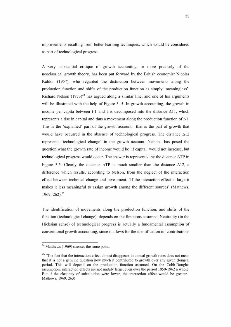
One problem with growth accounting is presented in Figure 3.5: income per capita (y)
and capital per worker (k) combinations A and B can be observed, but the underlying
production functions remain unobserved. The trick is to find a function that fits these
output-input combinations. Usually the Cobb-Douglas production function is used
(other functions are used less frequently Solow 1956, Kugler/Műller/ Sheldon 1990)
and the weights α and (1-α= β) are derived from the shares of capital and labor in
overall income.18 Since the shares of profit and labor add up to one, constant returns
to scale are assumed. Usually, α is assumed to be 1/3, a share derived from the
observed share of profits and labor in national income, which has turned out to be
more or less constant.
Figure 3.5: Growth Accounting
Y/L
K/L
Yt/L = F(Kt/L, 1)
Yt-1/L
Kt-1/L
Yt-1/L = F(Kt-1/L, 1)
Kt/L
Yt/L
A
B
C ∆12
∆11
∆TP
18 In a perfect market with profit maximization, factors are paid their marginal product. Thus, in a perfect market, the shares of labor income and capital income in overall income represent the weights α, (1-α) respectively.

27
Growth accounting studies estimated first which share of economic growth could be
attributed to the 'crude' input factors, capital and labor, and then identified the
unexplained part as technological progress. One of the first growth accounting efforts
was undertaken by Professor Jan Tinbergen (Tinbergen, 1942 #291), who generalized
the Cobb-Douglas production function by including a time-trend that represented
technological advancement.19 Using the weights that Douglas had found for capital
and labor (0.333 and 0.666 respectively), Tinbergen estimated that 100% of the
increase in output per person in Germany, Great Britain, France and the US could be
attributed to technological improvements (cited according to Griliches 1996). Later,
Salomon Fabricant (Fabricant, 1954 #292) estimated that in the US economy 92% of
the increase in output per person resulted from technological change or increased
efficiency. Abramovitz (1956) estimated a residual that was almost exactly the same
as Solow’s residual (1957), which was almost 90% of the experienced growth. Efforts
have subsequently been made to split the residual into different components, because
input factors are not homogenous over time, and improve in quality.
The quality of inputs, for example, is not constant over time. Labor, usually measured
in persons or hours, can change in skill content, and better skilled labor can be
expected to be more productive20. Thus, if workers become more skilled over time,
which has definitely been the case, but labor input is only measured in persons or
hours, the contribution of technological change (the residual) to income growth will
be overestimated. Similarly, new machines may be more productive than old
machines. If such changes in the quality of inputs are ignored, the residual
(technological progress) will be overestimated in the growth equation. Many studies
have consequently been carried out to adjust for quality changes in input factors.
These studies are known as the growth accounting literature, which has not only
19 Tinbergen used the formula: t= y - 2/3n - 1/3 k, where y, n and k are the average growth rates of output, labor, and capital, and he used explicitly the weights found by Douglas (see: (Griliches, 1996 #255):1326). 20 Labor is just one example of how difficult it is to disentangle variables. Why, for example, are higher skilled workers more productive? High skilled workers are hardly ever used for the same jobs as lower skilled workers. Consequently, the organization of the production process, and the machinery used, will not be same for high and low skilled labor. This indicates that the effects of labor on differences in productivity should not be attributed to only one factor, but rather to a combination of factors, as Richard Nelson (1973) argued.

28
succeeded in reducing the residual substantially, but also in identifying a significant
part of the residual.
Angus Madison (1996) computed estimates of the components of economic growth,
which are shown in Table 3.1. He used a similar method as Tinbergen, that is he
assumed the weights of labor and capital to be slightly different, 0.7 and 0.3
respectively, he assumed constant returns to scale. Madison’s estimates are
particularly interesting, because they have been calculated for six different countries
and have been divided into a period before 1973 and a period after. It has already
been discussed that economic growth in these two periods differed substantially, and
growth accounting may help to explain this difference. Some authors argue that the
main achievement of growth accounting is that it has stimulated the debate and
careful thinking about the variables that influence economic growth, rather than about
the method itself.
In his growth account, Madison distinguishes 3 components of labor input (hours
worked, education and labor dishoarding, which is only relevant for Japan and
Germany for the period after WWII), 3 categories of capital input (non-residential
capital capacity reactivation, which again is only relevant for Japan and Germany for
the post-war period, and an age effect) and 4 other variables: foreign trade, catch-up
effect, structural effect and economies of scale.
Only to the US, and mainly for the period after 1973, does Madison assign high
values to labor inputs. Additional hours of work are thought to contribute twice as
much as the rise in education, which is nevertheless substantial. Apart from Japan,
the US is the only country where hours worked (which is the combined effect of
average working hours and persons working) have increased. This is remarkable since
Madison’s hours estimates for the US are substantially below the OECD estimates
(compare …). In all other countries hours have declined. Therefore, the contribution
of rising educational attainment has been relatively more important for economic
growth in these countries. The trend for capital has been the reverse of the trend for
labor. Rising capital stock has contributed little in the US, whereas it has been the
largest source of GDP growth in all other countries. According to Madison’s

29
estimates, the age structure of capital has contributed little to GDP growth and its
contribution has declined since 1973. This may be because economic activity has
been lower since 1973 and that this has slowed down investment (see also Griliches
1988).
Remarkably, in some countries and periods, the 4 other variables (foreign trade,
catch-up effect, structural effect, and economies of scale) were equally important for
growth as capital. What is the rationale behind the inclusion of these other variables?
Economies of scale are ‘not included in strict neoclassical growth accounts which
assume constant returns to scale’ (Madison 1996: 62), but they were included in
Denison’s growth accounting.21 Madison’s economies of scale effect merely reflect
an assumption he made. However, it is equally arbitrary to assume ‘constant returns’
although it is consistent with the assumption of diminishing marginal productivity of
an increase in a single factor of production. However, this assumption does not
necessarily hold and this has led to an ever-increasing literature on ‘endogenous’ or
‘new’ and ‘evolutionary’ growth theory (see Chapters 4 and 5).
What are the consequences of making wrong assumptions about returns to scale? If
returns to scale are underestimated, for example, if they are actually greater than one
but in the model are taken to be one, then the contribution of input factors is
underestimated and the contribution of technological progress is overestimated. If, in
contrast, returns to scale are assumed to be higher then they actually are,
21 Since Adam Smith, economies of scale have been thought of as the key to raising productivity. They have first been included in growth accounting by Denison (1967 #218). Denison's reasoning was the following: countries with higher output achieve greater efficiency in production, and since income elasticities favor different goods, the richer countries will have economies of scale in the production of goods that are relatively more demanded at higher income levels (so called Luxuries). Thus, as the poorer countries catch up with the richer ones, their price structure will also catch up, meaning that their price structure, will become more similar because of economies of scale (‘luxuries’ decrease in relative price). Denison (1967 #218) attributed 40% of higher growth rates in France, Germany and Italy, over the period 1950 to 1962, to economies of scale, 11% to the adjustment of the European price structure to the US price structure and 30% to economies of scale related to income elasticities. Similar proportions have been estimated for the catch up of Japan to the US. In Box 3.5 it is shown that differences in price structure can influence the rates of economic growth.

30
technological progress will be underestimated and the contribution of input factors
will be overestimated.22
Table 3.1: Madison’s Growth Accounts for 6 Countries and 2 Periods (annual
average percentage point contribution to GDP growth rate)
France Germany Japan 1950-73 1973-92 1950-73 1973-1992 1950-73 1973-92 GDP 5.02 2.26 5.99 2.30 9.25 3.76 Hours worked .01 -.32 .00 -.27 1.01 .43 Education .36 .69 .19 .12 .52 .46 Labor dishoarding .00 0.00 .32 .00 .88 -.11 Non-residential capital 1.44 1.30 1.89 1.01 2.76 2.04 Capacity reactivation 0.00 0.00 .19 .00 .38 .00 Age effect .15 -.04 .12 -.08 -.08 -.07 Foreign trade .37 .12 .48 .15 .53 .09 Catch-up effect .46 .31 .62 .31 .98 .39 Structural effect .36 .15 .36 .17 1.22 .20 Economies of scale .15 .07 .18 .07 .28 .11 Growth explained 3.30 2.28 4.35 1.48 8.64 3.54 Growth unexplained 1.72 -.02 1.64 .82 .61 .22 Percentage explained 66 101 73 64 93 94 Labor 7 16 9 -7 26 21 Capital 32 56 37 40 33 52 Others 27 29 27 30 33 21 Netherlands UK US 1950-73 1973-92 1950-73 1973-1992 1950-73 1973-92 GDP 4.74 2.14 2.96 1.59 3.91 2.39 Hours worked -.05 -.05 -.11 -.40 .81 .86 Education .43 .57 .13 .42 .48 .43 Labor dishoarding .00 .00 /00 .00 .00 .00 Non-residential capital 1.37 .88 1.55 .99 .98 .94 Capacity reactivation .00 .00 .00 .00 .00 .00 Age effect .13 -.06 .09 -.06 .07 -.04 Foreign trade 1.32 .32 .32 .15 .11 .05 Catch-up effect .41 .24 .08 .20 .00 .00
22 This is clearly demonstrated by comparing the restricted (returns to scale equal one) and the unrestricted estimates of Michael Boskin and Lauwrence Lau (Boskin, 1992: 425), which show that estimates of technological progress are roughly twice as high for the unrestricted estimates as for the restricted estimates.
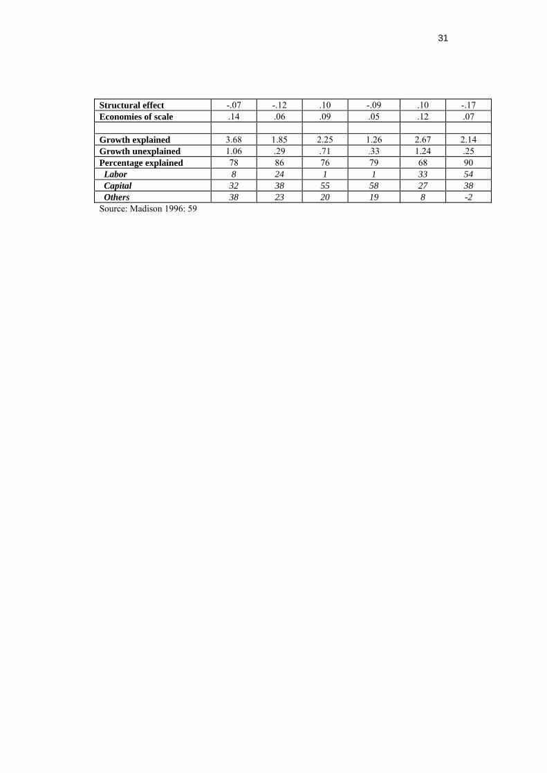
31
Structural effect -.07 -.12 .10 -.09 .10 -.17 Economies of scale .14 .06 .09 .05 .12 .07 Growth explained 3.68 1.85 2.25 1.26 2.67 2.14 Growth unexplained 1.06 .29 .71 .33 1.24 .25 Percentage explained 78 86 76 79 68 90 Labor 8 24 1 1 33 54 Capital 32 38 55 58 27 38 Others 38 23 20 19 8 -2 Source: Madison 1996: 59

32
Kaldor ((Kaldor, 1966 #122):13) has argued that the hypothesis of exogenous
productivity growth, that is, caused by progress in the knowledge of science and
technology, cannot explain why productivity growth in the car-industry was so much
higher in Germany than in Britain, given that the Americans owned a significant part
of the industry in both countries and both countries should have access to the same
technology. According to Kaldor, the hypothesis denies the existence of increasing
returns to scale, which are known to be an important feature of manufacturing
industries (Kaldor, 1966 # 122):13).
Criticisms of growth accounting are numerous. In neoclassical growth theory, for
example, there is no demand side (which has been regretted by Robert Solow, the
inventor of neoclassical growth theory) whereas in reality there are macroeconomic
influences on growth (as mentioned in Solow's Nobel lecture and as found by Edward
Wolff (1987),who has shown that international differences in investment rates explain
differences in technological progress, see Chapter 4). There is also microeconomic
feed back from demand to supply and vice versa. New products develop as a result of
the interaction between demand and supply and there is learning by using (Rosenberg
1996). If learning by using and learning by doing (Arrow 1961) are apparent, higher
economic activity (more investment) will provide more opportunities for learning,
and thus for more growth (this is one of the origins of endogenous growth theory, see
Chapter 4).
Does it make sense to control for changes in the quality of input factors? It is
debatable whether quality changes in input factors are really distinct from any other
form of technological progress. On the one hand, it can be argued that it requires
investments in human capital to raise the share of higher skilled labor, and thus that
labor with higher skills represents higher costs.23 On the other hand, it can be argued
that some improvements of skills do not require higher investments, for example,
23 Jorgensen et al. (1994) use wages as a reflection of differences in the quality of labor. This is an application of the assumption of profit maximization with competitive output and input markets that underlies many estimates.
33
improvements resulting from better learning techniques, which would be considered
as part of technological progress.
A very substantial critique of growth accounting, or more precisely of the
neoclassical growth theory, has been put forward by the British economist Nicolas
Kaldor (1957), who regarded the distinction between movements along the
production function and shifts of the production function as simply ‘meaningless’.
Richard Nelson (1973)24 has argued along a similar line, and one of his arguments
will be illustrated with the help of Figure 3. 5. In growth accounting, the growth in
income per capita between t-1 and t is decomposed into the distance ∆11, which
represents a rise in capital and thus a movement along the production function of t-1.
This is the ‘explained’ part of the growth account, that is the part of growth that
would have occurred in the absence of technological progress. The distance ∆12
represents ‘technological change’ in the growth account. Nelson has posed the
question what the growth rate of income would be if capital would not increase, but
technological progress would occur. The answer is represented by the distance ∆TP in
Figure 3.5. Clearly the distance ∆TP is much smaller than the distance ∆12, a
difference which results, according to Nelson, from the neglect of the interaction
effect between technical change and investment. ‘If the interaction effect is large it
makes it less meaningful to assign growth among the different sources’ (Mathews,
1969; 262).25
The identification of movements along the production function, and shifts of the
function (technological change), depends on the functions assumed. Neutrality (in the
Hicksian sense) of technological progress is actually a fundamental assumption of
conventional growth accounting, since it allows for the identification of contributions
24 Matthews (1969) stresses the same point. 25 ‘The fact that the interaction effect almost disappears in annual growth rates does not mean that it is not a genuine question how much it contributed to growth over any given (longer) period. This will depend on the production function assumed. On the Cobb-Douglas assumption, interaction effects are not unduly large, even over the period 1950-1962 a whole. But if the elasticity of substitution were lower, the interaction effect would be greater.” Mathews, 1969: 263)

34
by input factors, if these vary over time. If one would assume that technological
progress depends on input factors, one would not be able to identify these individual
contributions. For example, if a rise in capital input is accompanied by the
introduction of more productive and technologically advanced machinery (embodied
technological change) it would be impossible to determine which part of the increase
in production is due purely to higher capital inputs and which part is due to the use of
improved technology. The assumption of neutrality of technological progress has
long been debated and criticized: '[t]he use of more capital per worker inevitably
entails the introduction of superior techniques which require "inventiveness" of some
kind, though these need not necessarily represent the application of basically new
principles or ideas' (Kaldor, 1957 #5):595) (see also Arrow in Chapter 4). 'It follows
that any sharp or clear-cut distinction between the movement along a "production
function" with a given state of knowledge, and a shift of the "production function"
caused by a change in the state of knowledge is arbitrary and artificial' (Kaldor, 1957
#5):596).
The conclusions of growth accounting studies depend heavily on their underlying
assumptions. The most severe restrictions are: the assumed separability of individual
contributions to production (especially neutral technological change), profit
maximization in competitive output and input markets and constant returns to scale,
which implies diminishing returns to capital and labor. Growth accounting efforts
nevertheless contributed to the identification of the ingredients of inputs, although
they leave the process of innovation unexplained (exogenous) and are supply-side
biased. ‘Mono-causal or over-simple explanations are much less likely and much less
frequent with growth accounting than with regression analysis.’ (Madison 1996:57).

35
Box 3.5: The Impact of Price Structure on Growth Rates GDP is the sum of all goods and services produced in the economy in a certain period weighted with their pricces. If the price-structure between two countries differs, these two countries may have different GDP growth rates even if the quantities grow at exactly the same rates. We illustrate this relation with a simple example of two countries each with an identical two-sector economy in quantities but with different price structures.26 The GDP growth rate is the weighted average of the sectoral growth rates:
gGDP GDPGDP
gGDP at
t i it
i•
•=
•=
== − = ∑1
001 *
Where t is a time superscript, i is a sector subscript, a is the share of the sector in overall GDP. Now assume that overall GDP is identical in the two countries A and B and that the quantities produced in each sector is identical but that the price structure differs between the two economies in such a way that in country A the price level of sector 1 is twice as high as the price level of sector 2 and that in country B the reverse holds:
1 2 1 2A A BQ Q Q Q= = = B B
25; P P P PA A B1 2 12 0= =, .
The shares of sector 1 and 2 in overall GDP would then be the reverse in the two countries:
( )1 1
11 1 2 2
A AA
A A A A
Q PaQ P Q P
∗=
∗ + ∗
and because of the assumed relations above:
( )1 1
11 1 1 1
230.5
A AA
A A A A
Q PaQ P Q P
∗= =
∗ + ∗ ∗ and 1 1
3Aa =
respectively:
( )2 2
22 2 2 2
230.5
B BB
B B B B
Q PaQ P Q P
∗= =
∗ + ∗ ∗ and 1 1
3Ba =
26 Price structure between two economies may differ because of differences in natural resources or because of differences in size if there economies of scale.

36
I.e., the share in overall GDP in the two economies is the reverse only because the price structure differs. The quantity structure is identical. Now let the quantity in sector 1 in both economies grow with the same rate, say by factor 2. Quantities in sector 2 remain unchanged and prices do not change. We then get the following growth rates for overall GDP:
gGDPGDPGDP
aGDPGDP
aAAt
At A
At
At A= −
FHG
IKJ −
FHG
IKJ = + =
=
=
=
=,
,,
,
,,* * * * *1
1
10 1
21
20 21 1 1 2
30 1
323
gGDPGDPGDP
aGDPGDP
aBBt
Bt B
Bt
Bt B= −
FHG
IKJ −
FHG
IKJ = + =
=
=
=
=,
,,
,
,,* * * * *1
1
10 1
21
20 21 1 1 1
30 2
313
Although grows in quantity terms was exactly the same in the two economies, GDP (in constant prices) grows by two-third in country A but only by one-third in country B.