
Two- and three-dimensional few-body systems in the...
216
Two- and three-dimensional few-body systems in the universal regime Filipe Furlan Bellotti Department of Physics and Astronomy Aarhus University, Denmark ; Dissertation for the degree of Doctor of Philosophy October 2014
Transcript of Two- and three-dimensional few-body systems in the...

Two- and three-dimensional few-bodysystems in the universal regime
Filipe Furlan Bellotti
Department of Physics and Astronomy
Aarhus University, Denmark
;
Dissertation for the degree ofDoctor of Philosophy
October 2014

Filipe Furlan BellottiDepartment of Physics and AstronomyAarhus UniversityNy Munkegade, Bldg. 15208000 Arhus CDenmarkE-mail: [email protected]

This dissertation has been submitted to the Faculty of Science and Tech-nology at Aarhus University, Denmark, in partial fulfillment of the require-ments for the PhD degree in physics. The work presented has been per-formed in the period from August 2012 to July 2014 under the supervisionof Aksel S. Jensen from Aarhus University/Denmark and Tobias Fredericofrom Instituto Tecnologico de Aeronautica/Brazil. The work is the resultof an agreement on joint supervision of doctoral studies and was carriedout at the Department of Physics and Astronomy in Aarhus and at theDepartment for Natural Sciences in Sao Jose dos Campos.
”... A boy walks and walking he reaches the wall.
And there, right ahead, the future is waiting for us.
And the future is a spacecraft which we try to fly
It has neither moment, nor compassion, nor time to arrive.
Without asking permission it changes our lives and next it invites us to either
laugh or cry.
In this road, we are not supposed to either know or see what is coming.
Nobody does quite know for sure where it ends. ...”
— Toquinho / Vinicius de Morais / Maurizio Fabrizio / GuidoMorra
Free translation of part of Aquarela
iii


Acknowledgment
The project, which is ended by this thesis, has started approximately three
years ago. During the Master studies, my advisor Prof. Tobias Fred-
erico (ITA/Brazil) trusted and gave me the opportunity to visit Aarhus
University for three months. I have been very well received and the visit
was very fruitful. After getting my M.Sc. degree, Prof. Aksel S. Jensen
(AU/Denmark) proposed the joint supervision of the PhD studies. Since
then, I have two official advisors and I would like to thank them: Profs.
Tobias and Aksel. They have taught me about Physics, Mathematics, nu-
merical calculation, writing papers and reports, oral presentation, politics
in the academic area and other uncountable subjects. In practice, they have
given me guidelines to become a good, independent and honest Scientist.
Thank you so much for all the time spent and patience with me. I am very
proud in saying that you were my supervisors.
In practice, I had also three more advisors, who I should properly ac-
knowledge: Dmitri Fedorov and Nikolaj Zinner from from Aarhus University
(AU/Denmark) and Marcelo Yamashita from Instituto de Fısica Teorica
(IFT-UNESP/Brazil). They were always available to discuss about any
topic and their suggestions and comments have improved a lot my forma-
tion. In particular, Dmitri has always been exceptionally supportive during
my visits to Aarhus, as well as the secretaries Brigitte Henderson, Trine
Binderup and Karin Vittrup. They have always helped me with the admin-
istrative and logistic issues. A special thank goes for Tobias and Nikolaj for
having proofread the thesis.
The enjoyable time I had in Aarhus was in great extension due to the
company of Jeremy Armstrong, Artem Volosniev, Oleksandr Marchukov
and Jakob Knorborg, who were constantly present apart of the working
time.
v

At my work place in Brazil, Instituto de Fomento e Coordenacao Indus-
trial, I would like to firstly thank Cel. Eng. Augusto Luiz de Castro Otero,
who gave me conditions to study without quitting my job. I also appreciate
the support from my boss, Dr. Cesar Augusto Botura, and the advices from
Dr. Pedro Jose Pompeia.
My parents are the basis of my journey and they know how grateful I
am. The time spent in Aarhus has contributed a lot for my personal and
professional development, but it was one of the toughest periods I have ever
experienced, since I had to spent almost half of the first year of my daughter
away from my family. Therefore, the most special acknowledgement goes
to my beloved wife Monica, who has also passed through very hard times in
order to support me in this project. Without her support, this project would
not have been started, constructed and concluded. I am very thankful to
my young Cecilia, who has showed me that the mathematical and abstract
concept of infinity has a meaning: is the love I feel by her.
vi

Abstract
Macro properties of cold atomic gases are driven by few-body correlations,
even if the gas has thousands of particles. Quantum systems composed of
two and three particles with attractive zero-range pairwise interactions are
considered for general masses and interaction strengths in two and three
dimensions (2D and 3D). The Faddeev decomposition is used to derive the
equations for the bound state, which is the starting point for the inves-
tigation of universal properties of few-body systems, i.e. those that all
potentials with the same physics at low energy are able to describe in a
model-independent form. In 2D, the number of bound states in a three-body
system increases without bound as the mass of one particle becomes much
lighter than the other two. The analytic form of an effective potential be-
tween the heavy particles explains the mass-dependence on the number of
bound energy levels. An exact analytic expression for the large-momentum
asymptotic behavior of the spectator function in the Faddeev equation is
presented. The spectator function and its asymptotic form define the two-
and three-body contact parameters. The two-body parameter is found to
be independent of the quantum state in some specific 2D systems. The 2D
and 3D momentum distributions have a distinct sub-leading form whereas
the 3D term depends on the mass of the particles. A model that interpo-
lates between 2D and 3D is proposed and a sharp transition in the energy
spectrum of three-body systems is found.
vii

Resume
Makroskopiske egenskaber af ultrakolde atomare gasser styres af fa-legeme
korrelationer, det pa trods af at gassen har tusindvis af partikler. Vi studerer
kvantesystemer bestaende af to og tre partikler med attraktive to-partikel
vekselvirkninger med nul rækkevidde for generelle partikelmasser og vek-
selvirkningsstyrker i to og tre dimensioner (2D og 3D). Vi benytter Fad-
deev dekomposition til at udlede ligningerne for bundne tilstande, hvilket
er udgangspunktet for studier af universielle egenskaber ved fa-legeme sys-
temer. Dvs. de egenskaber som er uafhængig af den specifikke model for
potentialer der giver samme fysik ved lav energi. I 2D vokser antallet af
bundne tilstande i et tre-partikel system uden grænse nar en af de tre masser
er meget lettere end de andre to. Et analytisk udtryk for et effektivt po-
tential mellem de to tunge partikler kan forklare hvorledes antal bundne
energiniveauer afhænger af massen. Vi udleder et analytisk udtryk for
den sakaldte tilskuer-funktion fra Faddeev dekompositionen i den grænse
hvor impulsen bliver stor. Denne tilskuer-funktionen og den asymptotiske
opførsel benyttes til at bestemme to- og tre-partikel kontakt-parameteren.
To-partikel kontakt parameteren viser sig at være uafhængig af kvantetil-
stand i nogle bestemte 2D systemer. Impulsfordelingen i 2D og 3D har
en karakteristisk opførsel nar man betragter den første korrektion til den
ledende orden og i 3D far man her en korrektion der afhænger af massen
af partiklerne. Vi foreslar en model der interpolerer mellem 2D og 3D
grænserne og finder en veldefineret og skarp overgang i energispektret for
bundne tilstande af tre partikler.
ix


Contents
Acknowledgment v
Abstract vii
Resume ix
Table of Contents xiii
List of Publications xv
List of Figures xix
List of Tables xxi
1 Introduction 1
2 Two- and Three-body dynamics 72.1 Zero-range model and Renormalization . . . . . . . . . . . . . . 8
2.1.1 Two-body T-matrix in 2D . . . . . . . . . . . . . . . . . 102.1.2 Two-body T-matrix in 3D . . . . . . . . . . . . . . . . . 13
2.2 Notation and three-body dynamics . . . . . . . . . . . . . . . . 132.2.1 Three-body T-matrix . . . . . . . . . . . . . . . . . . . . 15
2.3 Three-body bound state equation in 2D . . . . . . . . . . . . . 182.4 Three-body bound state equation in 3D . . . . . . . . . . . . . 23
2.4.1 Renormalization of the 3B transition operator . . . . . 242.4.2 Three-body bound state integral equation in 3D . . . . 25
3 Universal 2D three-body bound states 273.1 Symmetry relations . . . . . . . . . . . . . . . . . . . . . . . . . 283.2 Survey of mass dependence . . . . . . . . . . . . . . . . . . . . . 293.3 Three-body energies for given masses . . . . . . . . . . . . . . . 333.4 Parametrization of three-body energies . . . . . . . . . . . . . . 36
4 Adiabatic approximation 414.1 Adiabatic potential . . . . . . . . . . . . . . . . . . . . . . . . . . 424.2 Asymptotic expressions . . . . . . . . . . . . . . . . . . . . . . . 464.3 Numerical results . . . . . . . . . . . . . . . . . . . . . . . . . . . 494.4 Estimate of the number of bound states . . . . . . . . . . . . . 51
xi

5 Momentum distribution in 2D 55
5.1 Asymptotic spectator function . . . . . . . . . . . . . . . . . . . 57
5.1.1 Parameterizing from small to large momenta . . . . . . 63
5.2 Asymptotic one-body densities . . . . . . . . . . . . . . . . . . . 64
5.2.1 Asymptotic contribution from n1(qα) . . . . . . . . . . 66
5.2.2 Asymptotic contribution from n2(qα) . . . . . . . . . . 66
5.2.3 Asymptotic contribution from n3(qα) . . . . . . . . . . 67
5.2.4 Asymptotic contribution from n4(qα) . . . . . . . . . . 70
5.2.5 Asymptotic contribution from n5(qα) . . . . . . . . . . 70
5.3 Contact parameters . . . . . . . . . . . . . . . . . . . . . . . . . 72
5.3.1 Analytic expressions . . . . . . . . . . . . . . . . . . . . 72
5.3.2 Identical Bosons . . . . . . . . . . . . . . . . . . . . . . . 74
5.3.3 Mass-imbalanced systems . . . . . . . . . . . . . . . . . 78
5.4 Discussion about possible experiments . . . . . . . . . . . . . . 85
6 Momentum distribution in 3D 87
6.1 Formalism and definitions . . . . . . . . . . . . . . . . . . . . . . 88
6.2 Asymptotic spectator function . . . . . . . . . . . . . . . . . . . 90
6.2.1 Scaling parameter . . . . . . . . . . . . . . . . . . . . . . 93
6.3 Asymptotic one-body densities . . . . . . . . . . . . . . . . . . . 95
6.4 Leading and sub-leading terms . . . . . . . . . . . . . . . . . . . 97
6.5 Numerical examples . . . . . . . . . . . . . . . . . . . . . . . . . 101
7 Dimensional crossover 105
7.1 Renormalization with a compact dimension . . . . . . . . . . . 107
7.2 3D - 2D transition with PBC . . . . . . . . . . . . . . . . . . . 109
7.2.1 Two-body scattering amplitude . . . . . . . . . . . . . 109
7.2.2 Dimer binding energy . . . . . . . . . . . . . . . . . . . 112
7.2.3 Trimer bound state equation . . . . . . . . . . . . . . . 114
7.3 2D - 1D with PBC . . . . . . . . . . . . . . . . . . . . . . . . . 115
7.3.1 Two-body scattering amplitude . . . . . . . . . . . . . . 116
7.3.2 Trimer bound state equation . . . . . . . . . . . . . . . 117
7.4 Trimer at 3D - 2D crossover with PBC . . . . . . . . . . . . . . 118
8 Summary and outlook 121
A Revision of the scattering theory 131
A.1 Brief presentation of the quantum scattering . . . . . . . . . . 131
A.2 Scattering equation for the two-body T-matrix . . . . . . . . . 134
xii

B Jacobi relative momenta 137B.1 Classical three-body problem . . . . . . . . . . . . . . . . . . . . 137B.2 Jacobi relative momenta . . . . . . . . . . . . . . . . . . . . . . 139
C Matrix elements of the three-body resolvent 143
D Numerical methods 147D.1 Three-body energy (eigenvalue) . . . . . . . . . . . . . . . . . . 147D.2 Spectator functions (eigenvector) . . . . . . . . . . . . . . . . . 154
E Asymptotic one-body density in 3D 157E.0.1 Asymptotic contribution from n1(qB) . . . . . . . . . . 157E.0.2 Asymptotic contribution from n2(qB) . . . . . . . . . . 157E.0.3 Asymptotic contribution from n3(qB) . . . . . . . . . . 159E.0.4 Asymptotic contribution from n4(qB) . . . . . . . . . . 167
F Detailed calculation of the residue 177
Bibliography 194
xiii


List of Publications
Bellotti, F. F.; Frederico, T.; Yamashita, M. T.; Fedorov, D. V.; Jensen, A.S.; Zinner, N. T. Scaling and universality in two dimensions: three-bodybound states with short-ranged interactions. Journal of Physics B , v.44, n. 20, p. 205302, 2011. Labtalk:http://iopscience.iop.org/0953-4075/labtalk-article/47307.
Bellotti, F. F.; Frederico, T.; Yamashita, M. T.; Fedorov, D. V.; Jensen, A.S.; Zinner, N. T. Supercircle description of universal three-body states intwo dimensions. Physical Review A, v. 85, p. 025601, 2012.
Bellotti, F. F.; Frederico, T.; Yamashita, M. T.; Fedorov, D. V.; Jensen,A. S.; Zinner, N. T. Dimensional effects on the momentum distribution ofbosonic trimer states. Physical Review A, v. 87, n. 1, p. 013610, Jan.2013.
Bellotti, F. F.; Frederico, T.; Yamashita, M. T.; Fedorov, D. V.; Jensen, A.S.; Zinner, N. T. Mass-imbalanced three-body systems in two dimensions.Journal of Physics B, v. 46, n. 5, p. 055301, May 2013. Labtalk:http://iopscience.iop.org/0953-4075/labtalk-article/52615.
Yamashita, M. T.; Bellotti, F. F.; Frederico, T.; Fedorov, D. V.; Jensen, A.S.; Zinner, N. T. Single-particle momentum distributions of efimov statesin mixed-species systems. Physical Review A, v. 87, p. 062702, Jun 2013.
Bellotti, F. F.; Frederico, T.; Yamashita, M. T.; Fedorov, D. V.; Jensen, A.S.; Zinner, N. T. Contact parameters in two dimensions for general three-body systems. New Journal of Physics, v. 16, n. 1, p. 013048, 2014.
Bellotti, F. F.; Frederico, T.; Yamashita, M. T.; Fedorov, D. V.; Jensen,A. S.; Zinner, N. T. Mass-imbalanced three-body systems in 2d: Boundstates and the analytical approach to the adiabatic potential. Few-BodySystems, v. 55, p. 847, 2014.
Bellotti, F. F.; Frederico, T.; Yamashita, M. T.; Fedorov, D. V.; Jensen, A.S.; Zinner, N. T. Universality of three-body systems in 2d: Parametrizationof the bound states energies. Few-Body Systems, v. 55, p. 1025, 2014.
xv

Yamashita, M. T.; Bellotti, F. F.; Frederico, T.; Fedorov, D. V.; Jensen, A.S.; Zinner, N. T. Dimensional crossover transitions of strongly interactingtwo- and three-boson systems. ArXiv e-prints, Apr. 2014.
xvi
List of Figures
2.1 Jacobi relative momenta . . . . . . . . . . . . . . . . . . . . . . 15
3.1 Mass diagram of the number of three-body bound states as
functions of two mass ratios, mb
maand mc
ma. The three two-body
energies are equal, i.e., Eab = Ebc = Eac. . . . . . . . . . . . . . . 30
3.2 Mass diagram of the number of three-body bound states as
functions of two mass ratios, mb
maand mc
ma. The two-body en-
ergies are Eab = 0 and Eac = Ebc. . . . . . . . . . . . . . . . . . . 31
3.3 Mass diagram of the number of three-body bound states as
functions of two mass ratios, mb
maand mc
ma. The two-body en-
ergies are Eab = 10Eac and Ebc = 0.1Eac. . . . . . . . . . . . . . 33
3.4 Contour diagrams with lines of fixed ǫ3 values as function of
the two-body energies ǫac and ǫbc. . . . . . . . . . . . . . . . . . 35
3.5 The functions, R0 and R1, of the three-body energy ǫ3 in the
super-ellipse fit for three sets of mass ratios. . . . . . . . . . . 37
3.6 The exponents, t0 and t1, in the super-ellipse fit as functions
of the three-body energy ǫ3 for three sets of mass ratios. . . . 38
4.1 Three-body relative coordinates used in the adiabatic ap-
proximation. . . . . . . . . . . . . . . . . . . . . . . . . . . . . . . 43
4.2 Ratio ǫasymptotic(s)/ǫexact(s) as function of the dimensionless
coordinate s(R), showing the validity of asymptotic expres-
sions. . . . . . . . . . . . . . . . . . . . . . . . . . . . . . . . . . . 47
4.3 Adiabatic potential ∣ǫasymptotic(R)/E2∣ as function of the di-
mensionless coordinate s(R). . . . . . . . . . . . . . . . . . . . . 48
4.4 Number of possible bound states (NB) for a system with mass
ratio m and Eab = 0. Comparison between the adiabatic ap-
proximation and the full solution of the set of coupled homo-
geneous integral equations. . . . . . . . . . . . . . . . . . . . . . 51
xvii

4.5 Number of possible bound states (NB) for a system with mass
ratio m for Eab = 0 and Eab = 1. . . . . . . . . . . . . . . . . . . 53
5.1 Spectator function, f(q), for the ground state calculated nu-
merically and using the ansatz f(q) = A0ln q
q2. . . . . . . . . . . 57
5.2 The difference fα (q)− Γ
mβγ
ln q
q2as a function of the momentum
q for three different systems. . . . . . . . . . . . . . . . . . . . . 61
5.3 Ratios between the three distinct spectator function for a
generic case of three distinct particles. . . . . . . . . . . . . . . 62
5.4 Comparison between the analytic spectator function estimated
for the ground state given and the numeric solution of the set
of coupled homogeneous integral equations. . . . . . . . . . . . 64
5.5 LO momentum distribution tail, q4n(q), for ground and ex-
cited three-body states. . . . . . . . . . . . . . . . . . . . . . . . 75
5.6 NLO momentum distribution comparison of 3D and 2D. . . . 78
5.7 The leading order term of the one-body momentum density
divided by En3for each bound state labeled as n. . . . . . . . . 81
5.8 The two-body parameters Caa and Cac as function of the mass
ratio m. . . . . . . . . . . . . . . . . . . . . . . . . . . . . . . . . 82
5.9 Comparison between the analytic estimative and numerical
calculation of Caa. . . . . . . . . . . . . . . . . . . . . . . . . . . 83
5.10 The sub-leading order of the one-body momentum density
divided by En3for each bound state labeled as n. . . . . . . . . 85
6.1 Comparison between the numerical solution of the set of cou-
pled homogeneous integral equations and the asymptotic for-
mula of fhe spectator function χAA(q). . . . . . . . . . . . . . . 92
6.2 Scaling parameter s as a function of the mass ratio A for
EAA = 0 (resonant interactions) and with no interaction be-
tween AA. . . . . . . . . . . . . . . . . . . . . . . . . . . . . . . . 95
6.3 C/κ0 for mass ratios in the range 6/133 ≤ A ≤ 25. . . . . . . . . 98
6.4 Non-oscillatory contributions for n1, n2, n3 and n4 as a func-
tion of the mass ratio A. . . . . . . . . . . . . . . . . . . . . . . 99
xviii

6.5 Individual non-oscillatory contributions for n1, n2, n3 and n4
as a function of the mass ratio A. . . . . . . . . . . . . . . . . . 1006.6 Scaling plot of the Efimov states indicating the points where
the momentum distributions have been calculated. . . . . . . . 102
6.7 Momentum distribution for the second excited state as a
function of the relative momentum of one particle to the CM
of the remaining pair. . . . . . . . . . . . . . . . . . . . . . . . . 103
6.8 Rescaled momentum distribution for the ground, first and
second excited states as a function of the relative momenta
of one particle to the CM of the remaining pair. . . . . . . . . 104
7.1 Dimensional crossover of the three-body binding energy spec-
trum. . . . . . . . . . . . . . . . . . . . . . . . . . . . . . . . . . . 119
A.1 Schematic figure showing the quantum scattering process. . . 131
B.1 Three-body coordinates in laboratory frame. . . . . . . . . . . 138
B.2 Relation of the new coordinates with the coordinates in frame
of the laboratory. . . . . . . . . . . . . . . . . . . . . . . . . . . . 140
E.1 Closed path used in the calculation of complex integrals. . . . 163
xix


List of Tables
5.1 The coefficients Cac
E3, Caa
E3and 2π
E3∫ ∞0 dk k ∣fc(k)∣2. . . . . . . . . 81
xxi


Chapter 1
Introduction
In the last decade scientists around the world found experimental evi-
dences [Kraemer 2006,Ferlaino 2010] of a remarkable phenomenon in few-
body systems that was predicted long time ago [Efimov 1970] and today is
known as the Efimov effect. It corresponds to an accumulation of three-
boson energy levels when the two-body scattering length tends to infin-
ity. In the exact limit - when the dimer energy is zero - the energies of
successive states are geometrically spaced obeying a universal ratio. Ex-
periments [Kraemer 2006] were able to identify few of these Efimov states,
bringing the attention of the physics community to few-body problems of
short-ranged interactions with large scattering lengths.
The experiments were realized using Feshbach resonances in cold atomic
gases (see, e.g., Ref. [Chin 2010]). Using this technique it is possible to
tune the scattering length to large values bringing the system into a uni-
versal regime, where their properties are essentially model-independent. In
this regime the properties of the system are defined by the knowledge of
only few physical low-energy observables that the short-ranged potentials
should produce. The possibility of manipulating the interaction between
trapped cold atoms also opened new avenues to probe few-body physics
as, for example, by studying systems restricted to two dimensions [Mar-
tiyanov 2010,Frohlich 2011,Dyke 2011]. Mostly, the theoretical background
in few-body physics was built for systems in three dimensions. However, the
experimental possibility to squeeze one of the dimensions, forming trapped
atomic systems in layers, asks for deeper and larger theoretical investiga-
tions of lower dimensional few-particle systems.
The number of spatial dimensions plays an important role in quantum
1
2
systems. For instance, let us consider the kinetic energy operator written in
angular coordinates. The dependence on the angle variables comes through
the centrifugal barrier operator, that in three dimensions has eigenvalues
always zero or positive, while in two dimensions, for zero angular momen-
tum, it is negative. This means that a minimum amount of attraction
is necessary to bind a three dimensional system, while any infinitesimal
attractive potential produce a s−wave bound state in a two dimensional
system [Nielsen 1997,Nielsen 1999,Nielsen 2001]. In fact this was already
pointed out a long time ago. The Landau criterion says that potentials
with negative volume integral will produce a bound state for any value
of the strength in two-dimensions (see, e.g., Ref. [Landau 1977]). This
topic continues to be of interest and it was found that when the volume
integral is exactly zero a bound state is still present [Simon 1976, Arm-
strong 2010,Volosniev 2011].
All this recent effort towards the two dimensional (2D) physics is sup-
ported by the relevance of the field for several different applications like,
e.g., high-temperature superconductors, localization of atoms on surfaces,
in semi-conducting micro-cavities, for carbon nanotubes and organic in-
terface. There is an interest among the ultracold atomic gas laboratories
to produce quantum degenerate gases in low dimensions, with the aim to
probe the two-dimensional physics of quantum systems. Early experiments
already produced quasi-2D samples of 133Cs [Vuletic 1998,Morinaga 1999,
Hammes 2003], 23Na [Gorlitz 2001], and 87Rb [Burger 2002]. Two-dimen-
sional gases with mixtures of 40K and 87Rb have been produced [Mod-
ugno 2003,Gunter 2005] and two-component gases of 6Li [Dyke 2011,Mar-
tiyanov 2010] and 40K [Frohlich 2011] have also been studied. Quasi-2D
pancakes of trapped heteronuclear diatomic molecules of 40K87Rb were pro-
duced in stacked layers [de Miranda 2011].
Theoretically one can define precisely the dynamics of quantum systems
in two-dimensions, while in a real experiment the confinement to 2D is
typically done using an optical lattice. This introduces a transverse energy
scale, hω0, and below it the physics is effectively 2D, while it becomes 3D at

CHAPTER 1. INTRODUCTION 3
or above hω0. To produce a 2D sample of trapped atoms in an experimental
setup, one starts with a three dimensional system. Therefore, it is important
to find observables that make possible to distinguish experimentally when
the system can be considered really in two dimensions.
The work consists in the study of two- and three- dimensional (2D and
3D) few-body systems close to the universal regime, where the world “uni-
versal”, which is extensively used along the work, means that the discussed
properties of the quantum systems are independent of the model utilized to
describe the interaction between two particles, namely, the weakly bound
system is much larger than the size of the interaction. A natural way to
study such properties is to describe the pairwise interaction with Dirac−δpotentials, since the condition for universality ∣a∣/r0 ≫ 1, where a is the
scattering length and r0 the range of the potential, is always fulfilled.
The introduction/motivation to the work given in Chapter 1 are followed
by the derivation of the equations that describe the 2D and 3D dynamics
of two- and three-body systems interacting through zero-ranged potentials
in Chapter 2. Notice that the problem consists basically in the solution of
an eigenvalue-eigenvector problem, where the energy and the wave function
of the three-body system must be determined. However, the complexity of
the three-body problem, which does not have a closed solution even at the
classical level, leads the problem to be described for an elaborated set of
homogeneous coupled integral equations.
The behavior of three-boson systems changes remarkably from two to
three dimensions, since the dynamics and properties of quantum systems
drastically change when the system is restricted to different dimensions.
Two important examples illustrating the influence of the spatial dimen-
sion in the three-body sector are the Efimov effect [Efimov 1970] and the
Thomas collapse [Thomas 1935]. The Efimov states (see the beginning of
Chapter 1), which were predicted and observed for three identical bosons in
3D systems [Kraemer 2006,Ferlaino 2010], are absent in 2D even in the most
favorable scenario of mass-imbalanced systems [Lim 1980, Adhikari 1988].
Similarly, Thomas found in 1935 that the energy of a three identical bosons

4
system subjected to short-range pairwise interactions in 3D grows without
boundaries (collapses) when the range of the interaction approaches zero
(r0 → 0). Nevertheless, this effect was not observed in 2D systems yet. It
is shown in Ref. [Adhikari 1988] that both the Thomas collapse and the
Efimov effect are mathematically related to the same anomaly in the kernel
of the three-body equations and they take place whenever ∣a∣/r0 →∞. For
instance, starting with finite and non-null values of ∣a∣ and r0, the finite andwell-behaviored three-body spectrum will collapse when r0 → 0. On the
other hand, infinitely many weakly bound states will appear for ∣a∣ → ∞.
Notice that the condition ∣a∣/r0 →∞ is fulfilled in both cases.
The sparseness of information about 2D three-bosons system has mo-
tivated the systematic investigation of the universal properties of mass-
imbalanced systems using zero-range interactions in momentum space [Bel-
lotti 2011,Bellotti 2012] and the results are shown in Chapter 3. The focus
is particularly on the dependence of the three-body binding energy with
masses and two-body binding energies. The critical values of these param-
eters (masses and two-body binding energies) allowing a given number of
three-particle bound states with zero total angular momentum are deter-
mined in a form of boundaries in the multidimensional parametric space.
Besides the dependence of the three-particle binding energy on the parame-
ters be highly non-trivial, even in the simpler case of two identical particles
and a distinct one, this dependence is parametrized for the ground and first
excited state in terms of supercircles functions in the most general case of
three distinguishable particles, as also presented in Chapter 3.
The study of the universal properties of 2D three-body systems has
shown an increasing number of bound states for the decreasing mass of one
of the particles [Bellotti 2011,Bellotti 2012]. The situation where one par-
ticle is much lighter than the other two is suitably handled in the adiabatic
approximation, namely the Born-Oppenheimer (BO) approximation, which
is presented in Chapter 4. The adiabatic potential between the heavy parti-
cles due to the light one found as the solution of a transcendental equation
is mass-dependent and reveals an increasing number of bound states by

CHAPTER 1. INTRODUCTION 5
decreasing the mass of one of the particles [Bellotti 2013b]. Besides, an
asymptotic expression for the adiabatic potential is derived and is shown
that this analytic expression faithfully corresponds to the numerically cal-
culated adiabatic potential, even in the non-asymptotic region. The number
of bound states for a heavy-heavy-light system is estimated as a function of
the light-heavy mass ratio and infinitely many bound states are expected
as this ratio approaches zero. However, for finite masses only finite number
of bound states is always present.
While Chapters 2 and 3 are focused in the eigenvalue of the three-body
Hamiltonian problem, Chapters 5 and 6 are related to the eigenstate in
momentum space, constructed from the spectator function and giving the
momentum density. A key result presented in Chapter 5 is the derivation
of an analytical expression for the asymptotic behavior of the spectator
function large momentum of three-body systems in two dimensions [Bel-
lotti 2013a,Bellotti 2014]. This asymptotic behavior defines the one-body
large momentum density, which is a strong candidate as observable quantity
able to unequivocally determine whether the quantum system is restricted
to two or three dimensions [Bellotti 2013a]. The two- and three-dimensional
one-body momentum densities are discussed respectively in Chapters 5 and
6. Besides, the one-body density defines the two- and three-body contact
parameters, which relate few- and many-body properties of quantum atomic
gases [Tan 2008]. It is shown in Chapter 5 that the two-body contact param-
eter, which is the coefficient in the leading order in the large momentum
expansion of the one-body density, of specific 2D systems is a universal
constant, in the sense that it does not depend on the quantum level con-
sidered [Bellotti 2013a,Bellotti 2014]. The three-body contact parameter,
which is the coefficient in the sub-leading order in the large momentum
expansion of the one-body density is not found to be universal, but the
sub-leading functional form is independent of the mass of the constituents
in 2D. The same does not happen in 3D systems, where the functional form
of the sub-leading term in the one-body momentum density depends on the
mass [Yamashita 2013], as shown in Chapter 6. Furthermore, the discus-

6
sion of how the one-body momentum density can be used to determine the
dimensionality of the system is also made in Chapter 5.
As current experimental set ups are able to continuously squeeze one di-
mension in order to build 2D experiments (see for instance Ref. [Dyke 2011]),
it is interesting to find theoretical methods which are able to produce a con-
tinuous squeezing of one of the dimensions. In Chapter 7 it is presented
a method that allows to study the dimensional crossover transitions of
strongly interacting two- and three-bosons systems by continuously “squeez-
ing” one of the dimensions [Yamashita 2014]. The particles are placed in
a flat surface plus a transverse direction (compact dimension), which im-
poses the discretization of the momentum accordingly to the chosen type
of boundary conditions. Employing periodic boundary conditions in the
compact dimension, it is shown that a sharp transition occurs in the energy
spectrum of three-body system as the system is squeezed from 3D to 2D.
However, more studies are still necessary in order to relate the parameter
which dials between the different situations to real experiments.
Summary and outlook are presented in Chapter 8. In order to moti-
vate the reading, the beginning of Chapters 2 to 7 brings a brief motiva-
tion/introduction to the topic that will be discussed. Further details are
given in Appendices A to F.

Chapter 2
Two- and Three-body
dynamics
The surprisingly fast and ongoing technological advances, which permeate
our daily life, has also given tools for an extraordinary grow on the exper-
imental studies of cold atomic quantum gases. However, the cornerstone
in the study of quantum systems in laboratories is still the same: these
systems are probed through collision experiments.
In this way, the background tools for the theoretical understanding of
such experiments are given by the scattering theory and some concepts of
this theory are presented in the following. While, even for low density gases,
the experiments are taken with several thousands of particles, it turns out
that some macro properties of the systems are driven by two- and three-body
correlations. This work is focused on the universal properties of three-body
quantum systems, i.e., when the size of the system is much larger than the
range of the interaction between the particles. Such problem is already
challenging and interesting in itself, since there is no classical equivalent.
A brief presentation of the quantum theory of scattering for two-body
zero-range potentials is given in Appendix A and the focus here is only
on the concepts and equations that are needed in order to make the read-
ing of this thesis easier. More details are given in Appendices A, B and C.
Complete and formal descriptions of the scattering theory in the three-body
quantum problem are given, for instance, in Refs. [Schmid 1974,Mitra 1969].
The main point here is the derivation of the integral equations for the two-
and three-body transition matrix (T−matrix) when the particles are as-
sumed to interact through zero-range potentials. Although these potentials
7

8 2.1. ZERO-RANGE MODEL AND RENORMALIZATION
are not realistic, their importance in the study of two- and three-body quan-
tum systems is explained in the next section.
2.1 Zero-range model and Renormalization
The s−wave zero-range potentials have a separable operator form (see Eq.
(A.15))
V = λ ∣χ⟩ ⟨χ∣ (2.1)
and will be used to solve the two-body T−matrix (see Eq. (A.13))
t = V + V g0t , (2.2)
as shown in Appendix A.2. For a s−wave separable potential, the transitionmatrix is (see Eqs. (A.19) and (A.21))
t(E) = ∣χ⟩ τ(E) ⟨χ∣ (2.3)
with
τ(E) = ⎛⎝λ−1 −∫ dDpg(p)2
E − p2
2mred+ ıǫ⎞⎠−1. (2.4)
Despite of the fact that Eq. (A.21) holds for any generic separable potential
that has the operator form given in Eq. (A.15), no local potential has this
form besides the zero-range one.
Zero-range potentials are very interesting. Although they do not corre-
spond any realistic interaction, they allow to study the phenomenology and
to understand the driven physics, which dominates the properties of large
quantum systems, namely systems with size much larger than the range of
the potential. They guide our intuition on the expected behavior of the
quantum few-body systems, since any realistic short-range potential must
reproduce the results obtained with zero-range potential when the system
is very large.
The s−wave zero-range model is introduced through a Dirac−δ interac-

CHAPTER 2. TWO- AND THREE-BODY DYNAMICS 9
tion which is also called contact interaction. This means that the particles
only interact when they touch each other. Besides, the Dirac−δ potential
has the operator form given by Eq. (A.15). In configuration space, the
matrix element of a local potential V is written as
⟨R′∣V ∣R⟩ = V (R)δ(R′ −R) . (2.5)
The Dirac−δ potential is local and V (R) = λδ(R). So, Eq. (2.5) becomes
⟨R′∣V ∣R⟩ = λδ(R)δ(R′ −R) = λδ(R)δ(R′) , (2.6)
meaning that this potential is also separable.
In momentum space, the matrix element of the Dirac−δ potential for a
n−dimensional system is
⟨p′∣V ∣p⟩ = λ(2π)D ∫ dDR∫ dDR′eıp′⋅R′e−ıp⋅Rδ(R′)δ(R) = λ(2π)D . (2.7)
It is possible to redefine ∣χ⟩ ≡ (2π)n/2 ∣χ⟩ so that Eq. (2.7) is equal to
λ. In this way, the form factor ⟨χ∣ p⟩ = ⟨p∣ χ⟩ = g(p) is equal to one for the
Dirac−δ potential, as can be seen below
g(p) = ⟨p∣ χ⟩ = (2π)D/2∫ dDRe−ıp⋅R(2π)D/2 δ(R) = 1 . (2.8)
The form factor of the Dirac−δ potential in Eq. (2.8) introduces a diver-
gence in the momentum integration of Eq. (A.21). In 2D and 3D the diver-
gence can be treated by introducing a physical scale in the problem [Fred-
erico 2012], but another way to render finite the integral could be done by
introducing a cut-off. It was shown in Ref. [Yamashita 2004b] that both
methods are equivalent when the momentum cut-off is let to be infinite.
The scale is introduced by defining a physical value for the two-body
T−matrix , λR, in a subtracted energy point defined by E = −µ2. The
10 2.1. ZERO-RANGE MODEL AND RENORMALIZATION
T−matrix becomes
τR(−µ2) = λR(−µ2) , (2.9)
where the subscript R means renormalized, and λR(−µ2) is given by a phys-
ical condition.
Inserting the condition from Eq. (2.9) in the matrix element given by
Eq. (A.21) gives
τR(−µ2) = ⎛⎝λ−1 −∫ dDp1
−µ2 − p2
2mred
⎞⎠−1 = λR(−µ2) , (2.10)
which allows to express the bare strength λ as
λ−1 = λ−1R (−µ2) +∫ dDp1
−µ2 − p2
2mred
. (2.11)
A finite expression for the scattering amplitude is found by replacing λ,
as given in Eq. (2.11), into the matrix element in Eq. (A.21). The result is
τR(E)−1 = λ−1R (−µ2) +∫ dDp⎛⎝ 1
−µ2 − p2
2mred
− 1
E − p2
2mred+ ıǫ⎞⎠ . (2.12)
2.1.1 Two-body T-matrix in 2D
Considering only bound states, i.e., E < 0, the integral on the right-hand-
side of Eq. (2.12) for two-dimensional systems (D = 2) isI(E) = ∫ d2p
⎛⎝ 1
−µ2 − p2
2mred
− 1
E − p2
2mred
⎞⎠ = −4πmred ln⎛⎝√−E
µ2
⎞⎠ , (2.13)
and from Eqs. (2.12) and (2.13), the renormalized two-body T−matrix is
given by
τR(E)−1 = λ−1R (−µ2) − 4πmred ln⎛⎝√−E
µ2
⎞⎠ . (2.14)
For positive energies, i.e., E > 0 (scattering states), the scattering am-
plitude is obtained from the analytic continuation of Eq. (2.14) in the upper

CHAPTER 2. TWO- AND THREE-BODY DYNAMICS 11
complex semi-plane of E, as shown below:
τR(E)−1 = λ−1R (−µ2) − 4πmred ln⎛⎝√−E
µ2
⎞⎠ ,= λ−1R (−µ2) − 4πmred ln
⎛⎝√
E
µ2
⎞⎠ + 2π2 ı mred , (2.15)
where the choice −1 = e−ıπ is used due to the analytic continuation in the
upper half semi-plane of the energy.
The matrix elements of the transition operator in Eq. (A.20) are ex-
pressed as
⟨p′∣ tR(E) ∣p⟩ = τR(E) , (2.16)
and for the sake of notation simplicity, the subscript R will be suppressed
in the equations from now on, i.e., τR(E) ≡ τ(E), λR(−µ2) ≡ λ(−µ2) andtR(E) ≡ t(E).
Looking at the matrix element in Eq. (2.14), it is not straightforward
to identify the s−wave scattering phase-shift and cross-section for the zero-
range model, as they were presented in Ref. [Adhikari 1993]. In units of
h = 2mred = 1, Eq. (2.14) becomes
τ(E)−1 = λ−1(−µ2) − π ln(−Eµ2) , (2.17)
where the respective analytic continuation for E > 0 is given in Eq. (2.15).
Using that ⟨p′∣ t(E) ∣p⟩ = 2π ⟨p′∣ t(E) ∣p⟩, the matrix elements in Eq. (2.16)
are written as
⟨p′∣ t(E) ∣p⟩ = 2π
λ−1 − π ln ( Eµ2) + ıπ2
= 2
π (− cot δ2 + ı) , (2.18)
where the s−wave phase-shift for the zero-range model is defined as
cot δ2 = − 1
π2λ(−µ2) + 1
πln(E
µ2) . (2.19)

12 2.1. ZERO-RANGE MODEL AND RENORMALIZATION
Then, the two-dimensional scattering length, a2, is found to be
a2 = − 1
π2λ(−µ2) + 1
πln(µ2) = a2 + 1
πln(µ2) . (2.20)
Notice that the logarithmic term, which appears in the low energy expan-
sion, leads to an ambiguity in the definition of the scattering length in 2D,
which depends on the scale used to measure the energy. So, the binding
energy of the pair, EB, is chosen as the physical scale in the problem. The
bound state energy (E < 0) is the pole of Eq. (2.18), i.e.,
ln(−Eµ2) = 1
π2λ(−µ2) , (2.21)
which gives
E = −µ2e−a2 = e−a2 = EB . (2.22)
Remember that λ(−µ2) is the physical information which was introduced
in the two-body T−matrix integral equation to handle the ultraviolet diver-
gence. Then, the subtraction point µ2 can be choose as the physical scale
of the problem, i.e., µ2 = −EB, where the binding energy of the pair is the
zero of Eq. (2.14). This choice also fixes the value of λ(−µ2), namely
τ(E)−1 = λ−1(EB) − 4πmred ln⎛⎝√
E
EB
⎞⎠ = 0 , (2.23)
at the bound-state pole and therefore
λ−1(EB) = 0 . (2.24)
Finally, the renormalized 2D two-body T−matrix for the zero-range
model is
τ(E)−1 = −4πmred ln⎛⎝√−E
EB
⎞⎠ , (2.25)
which will be used in the calculation of the properties of three-body systems
in 2D.

CHAPTER 2. TWO- AND THREE-BODY DYNAMICS 13
2.1.2 Two-body T-matrix in 3D
The 3D equivalent of Eq. (2.12) is given by
τR(E)−1 = λ−1R (−µ2) +∫ d3p⎛⎝ 1
−µ2 − p2
2mred
− 1
E − p2
2mred+ ıǫ⎞⎠ , (2.26)
where, as before, E is the energy, µ2 the subtraction point, mred the reduced
mass and the subscript R means renormalized. For E < 0 (bound states),
the integral on the right-hand-side of Eq. (2.26) is
I(E) = ∫ d3p⎛⎝ 1
−µ2 − p2
2mred
− 1
E − p2
2mred
⎞⎠ = −4π2mred (√2mred∣E∣ −√2mredµ2) .(2.27)
As in the 2D case, the subtraction point is chosen as the two-body bind-
ing energy, i.e., −µ2 = EB and Eq. (2.24) also holds in the 3D case, namely
λ−1R (EB) = 0. Then, dropping the subscript R, the two-body T−matrix for
3D systems is given by
τ(E)−1 = −2π2 (2mred)3/2 (√∣E∣ −√∣EB ∣) , (2.28)
which will be used in the calculation of the properties of three-body systems
in 3D.
2.2 Notation and three-body dynamics
The system consists of three distinguishable particles of masses mα, mo-
menta kα and pairwise interactions vα, where α = a, b, c labels the particles
(a, b, c) and the notation of the potential is such that va is the interaction
between particles b and c. The eigenvalue equation for the Hamiltonian
(H0 + V )Ψ = EΨ , (2.29)

14 2.2. NOTATION AND THREE-BODY DYNAMICS
is fulfilled by states in the discrete (E < 0) and continuum (E > 0) regions.The potential given by two-body terms is V = va + vb + vc and the free and
full propagators are respectively given by
G0(Z) ≡ 1
Z −H0
and G(Z) ≡ 1
Z −H , (2.30)
with H = H0 + V . The free Hamiltonian, in frame of the laboratory, is
given by the sum over the individual kinetic energies of the particles and is
written as
H0 = ∑α=a,b,c
k2α2mα
. (2.31)
A set of Jacobi coordinates and the canonical conjugate momenta, which
are shown in Fig. 2.1, are useful when dealing with three-body problems,
since the CM motion is separated out. In this case the free Hamiltonian
becomes
H0 = p2α2mβγ
+ q2α2mβγ,α
+ Q2
mα +mβ +mγ
, (2.32)
where Q = ∑α kα is the CM momentum. Taking into account the frame of
particle α with respect to the CM of the pair (β, γ), qα is the momentum of
particle α with respect to the CM of the pair, pα is the relative momentum
of the pair, mβγ is the reduced mass of the pair and mβγ,α is the three-body
reduced mass. The relative momenta and reduced masses are given by
qα = mβ +mγ
mα +mβ +mγ
[kα − mα
mβ +mγ
(kβ + kγ)] , (2.33)
pα = mγkβ −mβkγ
mβ +mγ
, (2.34)
mβγ = mβmγ
mβ +mγ
, (2.35)
mβγ,α = mα (mβ +mγ)mα +mβ +mγ
, (2.36)
with (α,β, γ) as cyclic permutations of (a, b, c) (see Appendix B for more
details about Jacobi relative momenta). It is also useful to specify an op-
erator notation, where all two-body operators are represented with small

CHAPTER 2. TWO- AND THREE-BODY DYNAMICS 15
Figure 2.1: Jacobi relative momenta
letters, i.e., vα, g0 and three-particle operators are represented by capital
letters, i.e., H,V .
2.2.1 Three-body T-matrix
The three-body transition operator is written as
T (E) = V + V G (E + ıǫ)V , (2.37)
that is the formal analogue of the two-body T−matrix in Eq. (A.11). Besides
that the operator in Eq. (2.37) is not directly related to the scattering cross
section as in the two-body case, the relations in Eqs. (A.13) and (A.14) also
hold and read
T (E) = V + V G0(E + ıǫ)T (E) = V + T (E)G0(E + ıǫ)V . (2.38)
The Faddeev components of the three-body T−matrix (see Ref. [Fad-

16 2.2. NOTATION AND THREE-BODY DYNAMICS
deev 1965,Schmid 1974]) are given by
Ta(E) = va + vaG0(E + ıǫ)T (E) (2.39)
and since that V = va + vb + vc, the transition operator from Eq. (2.38) can
be written in term of the components given by Eq. (2.39) as
T (E) = Ta(E) + Tb(E) + Tc(E) . (2.40)
Inserting Eq. (2.40) back into Eq. (2.39) results in a system of coupled
equations, which are written in matrix form as
⎛⎜⎜⎜⎝Ta
Tb
Tc
⎞⎟⎟⎟⎠ =⎛⎜⎜⎜⎝va
vb
vc
⎞⎟⎟⎟⎠ +⎛⎜⎜⎜⎝va va va
vb vb vb
vc vc vc
⎞⎟⎟⎟⎠G0
⎛⎜⎜⎜⎝Ta
Tb
Tc
⎞⎟⎟⎟⎠ . (2.41)
Isolating the component Ta in Eq. (2.41) results in
(1 − vaG0)Ta = va + vaG0 (Tb + Tc) , (2.42)
which multiplied by (1 − vaG0)−1 from the left gives
Ta = ta + taG0 (Tb + Tc) , (2.43)
where the relation ta = [1 − vaG0]−1 va was used in third line. The renormal-
ized two-body T−matrix ta in the abc system is given by
ta ≡ ta(E) = ∣χa⟩ τa(E) ⟨χa∣ with τa(E)−1 = −4πmbc ln⎛⎝√−E
Ebc
⎞⎠ . (2.44)
Finally, the set of coupled equations for the Faddeev components of the

CHAPTER 2. TWO- AND THREE-BODY DYNAMICS 17
three-body transition operator are written in matrix form as
⎛⎜⎜⎜⎝Ta
Tb
Tc
⎞⎟⎟⎟⎠ =⎛⎜⎜⎜⎝ta
tb
tc
⎞⎟⎟⎟⎠ +⎛⎜⎜⎜⎝
0 ta ta
tb 0 tb
tc tc 0
⎞⎟⎟⎟⎠G0
⎛⎜⎜⎜⎝Ta
Tb
Tc
⎞⎟⎟⎟⎠ . (2.45)
These equations have the advantage to contain the only the two-body
T−matrix, and consequently two-body energies, instead of the potential.
The power of such formulation is better explained and explored in Chapter 3.
Besides, Eq. (2.45) shows how the two-body scattering amplitude connects
with the three-body scattering. In detail, the equation for one Faddeev
component of the transition operator is given by
Ta(E3) = ta (E3 − q2a2mbc,a
)⎧⎪⎪⎨⎪⎪⎩1 +G0(E3 + ıǫ)[Tb(E3) + Tc(E3)]⎫⎪⎪⎬⎪⎪⎭ , (2.46)
where E3 is the three-body energy and the other components are found by
cyclic permutation of the particle labels.
Notice that the argument of the two-body T−matrix in Eq. (2.15) is the
relative two-body energy, ER2, which was replaced by E3− q2
2mbc,ain Eq. (2.46).
The relative two-body energy connects with the total energy, ET2, through
ET2= ER
2+ q2
2
2(mb+mc) , where q2 is the total momentum of the pair. At the
frame of the CM in a three-body system, i.e., Q = 0, the total energy of
the pair is the difference between the three-body energy E3 and the kinetic
energy of the third particle, namely ET2= E3 − q2
1
2ma. Moreover, if Q = 0 the
momentum of the pair is exactly the momentum of the third particle. In
other words, ∣q1∣ = ∣−q2∣ = q and the relative two-body energy as function of
the three-body energy is written as
ER2 = E3 − q2
2ma
− q2
2 (mb +mc) = E3 − q2
2mbc,a
, (2.47)
which is exactly the argument of the two-body T−matrix in Eq. (2.46).

18 2.3. THREE-BODY BOUND STATE EQUATION IN 2D
2.3 Three-body bound state equation in 2D
The three-body T−matrix in Eq. (2.45) describes the three-body scatter-
ing process with pairwise short-range potentials. The transition operator
generally contains all the strong interaction properties of the three-body
system or, in other words, it allows to construct the resolvent of the inter-
acting model. Therefore, the T−matrix gives information about both bound
(E3 < 0) and scattering (E3 > 0) states. The focus in the following Chap-
ters is on three-body bound states, then the coupled homogeneous integral
equations for the bound state are derived here, starting from the transition
operator. It is possible to instead use directly the Faddeev decomposition
for the bound-state wave function [Mitra 1969].
The completeness relation is defined as
1 =∑B
∣ΦB⟩ ⟨ΦB ∣ +∫ d2k ∣Ψ(+)c ⟩ ⟨Ψ(+)c ∣ , (2.48)
where ∣ΦB⟩ and ∣Ψ(+)c ⟩ represent the wave functions of bound and scattering
states, respectively. The T−matrix (2.37), written in terms of the interacting
resolvent decomposed in eigenstates of H, is written as
T (E3) = V +∑B
V ∣ΦB⟩ ⟨ΦB ∣VE3 −EB + ıǫ +∫ d2k
V ∣Ψ(+)c ⟩ ⟨Ψ(+)c ∣VE − Ec + ıǫ , (2.49)
where the bound-state poles of the transition operator appear explicitly.
When the three-body system is close to a bound state (E3 ≈ EB), the second
term on the right-hand-side of Eq.(2.49) is dominant, due to the pole, and
the part concerning to the scattering states can be neglected. Defining the
bound state vertex function by ∣ΓB⟩ = V ∣ΦB⟩, the three-body T−matrix
(2.49) near the pole becomes
T (E3) ≈ ∣ΓB⟩ ⟨ΓB ∣E3 −EB
= ∣ΓB⟩ ⟨ΓB ∣E3 + ∣EB ∣ . (2.50)
Then, Eq. (2.50) is decomposed in three Faddeev components, as in Eq. (2.39),

CHAPTER 2. TWO- AND THREE-BODY DYNAMICS 19
which reads
Ta (E3) ≈ ∣Γa⟩ ⟨ΓB ∣E3 + ∣EB ∣ , (2.51)
where ∣Γa⟩ = va ∣ΦB⟩ and ⟨ΓB ∣ = ⟨ΦB ∣V . Inserting the T−matrix (2.51) in
Eq. (2.46) gives
∣Γa⟩ ⟨ΓB ∣E3 + ∣EB ∣ ≈ ta (E3 − q2a
mbc,a
)[1 +G0 (E3)( ∣Γb⟩ ⟨ΓB ∣E3 + ∣EB ∣ + ∣Γc⟩ ⟨ΓB ∣
E3 + ∣EB ∣)] . (2.52)
When the three-body system is bound, E3 → − ∣EB ∣ and in this limit
Eq. (2.52) becomes a homogeneous equation, which reads
∣Γa⟩ = ta (E3 − q2ambc,a
)G0 (E3) (∣Γb⟩ + ∣Γc⟩) . (2.53)
Writing the two-body T−matrix for the one term separable potential, as
in Eq. (A.19), gives
∣Γa⟩ = ∣χa⟩ τa (E3 − q2ambc,a
) ⟨χa∣G0 (E3) (∣Γb⟩ + ∣Γc⟩) , (2.54)
and the projection of Eq. (2.54) in states ∣pa,qa⟩ results in⟨pa,qa ∣Γa⟩ = ⟨pa ∣χa⟩ τa (E3 − q2a
mbc,a
) ⟨χa,qa∣G0 (E3) (∣Γb⟩ + ∣Γc⟩) . (2.55)
For Dirac−δ potentials, ⟨pa,qa∣ Γa⟩ = ⟨pa∣ χa⟩ ⟨qa∣ fa⟩ = ga (pa)fa (qa) =fa (qa) and the ith Faddeev component of the three-body bound state vertex,
which satisfies an homogeneous integral equation, is given by
fa (qa) = τa (E3 − q2a2mbc,a
) ⟨χa,qa∣G0 (E3) (∣χb⟩ ∣fb⟩ + ∣χc⟩ ∣fc⟩), (2.56)
where fa is the spectator function, which describes the interaction of each
spectator particle with the corresponding two-body subsystem. The specta-
tor functions fb and fc are easily found by cyclic permutation of the labels
(a, b, c) in Eq. (2.56).

20 2.3. THREE-BODY BOUND STATE EQUATION IN 2D
The components fa, fb and fc satisfy a set of three coupled homogeneous
integral equations, in the case where the interaction between particles is
described for zero-range potentials. For three identical bosons, only one
homogeneous integral equation has to be solved, since fa (qa) = fb (qb) =fc (qc). In the same way, for two identical bosons plus a distinct particle,
there is a set of two coupled homogeneous integral equations, since fa (qa) =fb (qb) ≠ fc (qc). In the most general case of three distinguishable particles,
the set of coupled equations reads
fa (qa) =τa (E3 − q2a2mbc,a
) ⟨χa,qa∣G0 (E3) (∣χb⟩ ∣fb⟩ + ∣χc⟩ ∣fc⟩) , (2.57)
fb (qb) =τb (E3 − q2b2mca,b
) ⟨χb,qb∣G0 (E3) (∣χa⟩ ∣fa⟩ + ∣χc⟩ ∣fc⟩) , (2.58)
fc (qc) =τc (E3 − q2c2mab,c
) ⟨χc,qc∣G0 (E3) (∣χa⟩ ∣fa⟩ + ∣χb⟩ ∣fb⟩) . (2.59)
The matrix elements in Eqs. (2.57) to (2.59) have the same structure,
namely
⟨χa,qa∣G0 (E3) ∣χb⟩ ∣fb⟩ . (2.60)
These matrix elements are derived in detail in Appendix C and the result is
used to finally write the set of three coupled homogeneous integral equations
for the bound state of an abc system as
fa (qa) =⎡⎢⎢⎢⎢⎢⎣−4π mbmc
mb +mc
ln⎛⎜⎝¿ÁÁÀ ma+mb+mc
2ma(mb+mc)q2a −E3
Ebc
⎞⎟⎠⎤⎥⎥⎥⎥⎥⎦−1×
× ⎡⎢⎢⎢⎣∫ d2kfb (k)
E3 − ma+mc
2mamcq2a − mb+mc
2mbmck2 − 1
mck ⋅ qa
+
+∫ d2kfc (k)
E3 −ma+mb
2mambq2a −
mb+mc
2mbmck2 − 1
mbk ⋅ qa
⎤⎥⎥⎥⎦ , (2.61)

CHAPTER 2. TWO- AND THREE-BODY DYNAMICS 21
fb (qb) =⎡⎢⎢⎢⎢⎢⎣−4π
mamc
ma +mc
ln⎛⎜⎝¿ÁÁÀ ma+mb+mc
2mb(ma+mc)q2b −E3
Eac
⎞⎟⎠⎤⎥⎥⎥⎥⎥⎦−1×
×
⎡⎢⎢⎢⎣∫ d2kfa (k)
E3 −mb+mc
2mbmcq2b −
ma+mc
2mamck2 − 1
mck ⋅ qb
+
+∫ d2kfc (k)
E3 −ma+mb
2mambq2b −
ma+mc
2mamck2 − 1
mak ⋅ qb
⎤⎥⎥⎥⎦ , (2.62)
fc (qc) =⎡⎢⎢⎢⎢⎢⎣−4π
mamb
ma +mb
ln⎛⎜⎝¿ÁÁÀ ma+mb+mc
2mc(ma+mb)q2c −E3
Eab
⎞⎟⎠⎤⎥⎥⎥⎥⎥⎦−1×
×
⎡⎢⎢⎢⎣∫ d2kfa (k)
E3 −mb+mc
2mbmcq2c −
ma+mb
2mambk2 − 1
mbk ⋅ qc
+
+∫ d2kfb (k)
E3 −ma+mc
2mamcq2c −
ma+mb
2mambk2 − 1
mak ⋅ qc
⎤⎥⎥⎥⎦ . (2.63)
The particles a, b and c have masses ma,mb,mc, respectively. Also, the
two-body bound state energy of each pair, defined as the scale factor of
the two-body system for Dirac−δ potentials (see Eq. (2.22)), is specifically
labeled as Eab, Ebc and Eac.
The spectator functions in Eqs. (2.61) to (2.63) compose the three-
body bound-state wave function. Using the vertex function defined before
Eq. (2.50), ∣ΓB⟩ = V ∣ΦB⟩ , it is possible to write that (va + vb + vc) ∣ΨB⟩ =∣Γa⟩ + ∣Γb⟩ + ∣Γc⟩. Multiplying both sides by the free resolvent results in
∣Ψabc⟩ = ∣Ψa⟩ + ∣Ψb⟩ + ∣Ψc⟩ = G0(E3)[∣Γa⟩ + ∣Γb⟩ + ∣Γc⟩] , (2.64)
where ∣Ψa⟩ = G0(E3)va ∣ΨB⟩ is one of the so-called Faddeev components of
the wave function. It is possible to choose any one of the set of Jacobi
momenta to project Eq. (2.64). The set (qa,pa) gives
⟨qa,pa∣ Ψabc⟩ = ⟨qa,pa∣G0(E3)(∣Γa⟩ + ∣Γb⟩ + ∣Γc⟩) . (2.65)

22 2.3. THREE-BODY BOUND STATE EQUATION IN 2D
The matrix elements on the right-hand-side of Eq.(2.65) can be handled in a
similar way as it is done in Appendix C. Finally, the three-body bound-state
wave function is written in term of the spectator functions as
Ψabc(qa,pa) = fa(qa) + fb(qb(qa,pa)) + fc(qc(qa,pa))E3 −
ma+mb+mc
2ma(mb+mc)q2a −
mb+mc
2mbmcp2a
, (2.66)
where the Jacobi momenta qb and qc are linearly related to qa and pa
through the relations given in Appendix B.
In a compact notation, (α,β, γ) are introduced as cyclic permutations
of the labels (a, b, c) and the wave function is written taking into account
the momentum of particle α with respect to the CM of the βγ subsystem
as
Ψ (qα,pα) = fα (qα) + fβ (∣pα −mβ
mβ+mγqα∣) + fγ (∣pα +
mγ
mβ+mγqα∣)
−E3 +q2α
2mβγ,α+
p2α2mβγ
, (2.67)
where qα,pα are the Jacobi momenta of particle α with the shifted argu-
ments given in Eqs. (B.31) and (B.32) and mβγ,α = mα(mβ +mγ)/(mα +
mβ +mγ) and mβγ = (mβ +mγ)/(mβ +mγ) are the reduced masses. In the
same way, the spectator functions in Eq. (2.67), i.e., fα,β,γ(q), fulfill the setof three coupled homogeneous integral equations for the bound state, which
in the compact notation are written as
fα (q) =⎡⎢⎢⎢⎢⎢⎢⎣4πmβγ ln
⎛⎜⎜⎝¿ÁÁÁÀ q2
2mβγ,α−E3
Eβγ
⎞⎟⎟⎠⎤⎥⎥⎥⎥⎥⎥⎦
−1(2.68)
×∫ d2k⎛⎜⎝
fβ (k)−E3 +
q2
2mαγ+
k2
2mβγ+
1
mγk ⋅ q
+fγ (k)
−E3 +q2
2mαβ+
k2
2mβγ+
1
mβk ⋅ q
⎞⎟⎠ .As the interaction between particles is described for s−waves potentials
and the focus is on states with total zero angular momentum, the spectator
functions do not depend on the angle, i.e., fα(q) ≡ fα(q). Then, the angular
CHAPTER 2. TWO- AND THREE-BODY DYNAMICS 23
integration in Eq. (2.68) is solved using that
∫2π
0
dθ
1 − z cos θ= 1√
1 − z2, (2.69)
where the constant z satisfies ∣z∣ < 1. The result is
fα (q) = 2π⎡⎢⎢⎢⎢⎢⎢⎣4πmβγ ln
⎛⎜⎜⎝¿ÁÁÁÀ q2
2mβγ,α−E3
Eβγ
⎞⎟⎟⎠⎤⎥⎥⎥⎥⎥⎥⎦
−1
×∫∞
0
dk
⎛⎜⎜⎜⎝k fβ (k)√(−E3 +q2
2mαγ+
k2
2mβγ)2 − ( k q
mγ)2
+k fγ (k)√(−E3 +q2
2mαβ+
k2
2mβγ)2 − ( k q
mβ)2⎞⎟⎟⎟⎠ , (2.70)
which together with Eq. (2.67) build the Ltotal = 0 bound eigenstate of the
Hamiltonian with the zero-range force.
The study of the three-body bound states, in what follows, is based on
the numerical solution of the coupled homogeneous integral equations for
the spectator functions in Eq. (2.70). Details about the numerical methods
are given in Appendix D.
2.4 Three-body bound state equation in 3D
The naive attempt to write the three-body bound state integral equation
in 3D only by changing the phase factor and the two-body T−matrix in
Eq. (2.68) fails, since the kernel of such equation is non-compact when
the interaction between particles is described for Dirac−δ potentials [Ad-
hikari 1988]. This means that the three-body equations must be renor-
malized, as it was done for the two-body T−matrix in Sec. 2.1. A com-
plete discussion about the renormalization method is given in Refs. [Ad-
24 2.4. THREE-BODY BOUND STATE EQUATION IN 3D
hikari 1995b, Adhikari 1995a, Frederico 2012], where a discussion of the
equivalent method within effective field theory can be found.
2.4.1 Renormalization of the 3B transition operator
The Lippmann-Schwinger equation for the transition operator is
T (E) = V + V G0(E)T (E) = V + T (E)G0(E)V , (2.71)
which for the sake of the notation the energy is dropped.
The subtraction point is chosen as −µ2(3) and the transition matrix in
this point is T (−µ2(3)). The potential V can be expressed as
V = [1 + T (−µ2(3))G0 (−µ2(3))]−1 T (−µ2(3)) , (2.72)
where T (−µ2(3)) is defined as the sum over the two-body transition matrices
in the subtraction point [Adhikari 1995b], namely
T (−µ2(3)) = ∑n=a,b,c
tn (−µ2(3)) , (2.73)
with tn(E) given in Eq. (2.44). Inserting the renormalized potential (2.72)
in Eq. (2.71) gives
T (E) = [1 + T (−µ2(3))G0 (−µ2(3))]−1 T (−µ2(3)) [1 +G0(E)T (E)] ,[1 + T (−µ2(3))G0 (−µ2(3))]T (E) = T (−µ2(3)) + T (−µ2(3))G0(E)T (E) ,T (E) + T (−µ2(3))G0 (−µ2(3))T (E) = T (−µ2(3)) + T (−µ2(3))G0(E)T (E) ,T (E) = T (−µ2(3)) + T (−µ2(3))G1 (E,−µ2(3))T (E) , (2.74)
where
G1 (E,−µ2(3)) = G0(E) −G0 (−µ2(3)) = −(µ2(3) +E)G0(E)G0 (−µ2(3)) .(2.75)

CHAPTER 2. TWO- AND THREE-BODY DYNAMICS 25
Notice that the matrix form of Eq. (2.74) is given in Eq. (2.45), meaning
that each component of the renormalized three-body transition matrix is
given by
Ta(E3) = ta (E3 −q2a
2mbc,a
)⎧⎪⎪⎨⎪⎪⎩1 +G1 (E3,−µ2(3)) [Tb(E3) + Tc(E3)]⎫⎪⎪⎬⎪⎪⎭ , (2.76)
which is analogous to Eq. (2.46), where the only difference arises from the
three-body propagator.
2.4.2 Three-body bound state integral equation in 3D
Since Eqs. (2.46) and (2.76) are equivalent, the procedure to obtain the
three-body bound state equation in 3D is exactly the same followed in
Sec. 2.3, only replacing G0(E3) → G1 (E3,−µ2(3)). Then, the homogeneous
coupled equations for the spectator function to get the bound state energy
are given by
fa (qa) =τa (E3 −q2a
2mbc,a
) ⟨χa,qa∣G1 (E3,−µ2(3))(∣χb⟩ ∣fb⟩ + ∣χc⟩ ∣fc⟩) ,
(2.77)
fb (qb) =τb (E3 −q2b
2mca,b
) ⟨χb,qb∣G1 (E3,−µ2(3))(∣χa⟩ ∣fa⟩ + ∣χc⟩ ∣fc⟩) ,
(2.78)
fc (qc) =τc (E3 −q2c
2mab,c
) ⟨χc,qc∣G1 (E3,−µ2(3))(∣χa⟩ ∣fa⟩ + ∣χb⟩ ∣fb⟩) .
(2.79)
Notice that the matrix elements in Eqs. (2.77) to (2.79) have the same
structure as the ones in Eqs. (2.57) to (2.59) , namely
⟨χa,qa∣G1 (E3,−µ2(3)) ∣χb⟩ ∣fb⟩ . (2.80)

26 2.4. THREE-BODY BOUND STATE EQUATION IN 3D
Since the termG1 (E3,−µ2(3)) can be separated in two terms, as in Eq. (2.75),
it turns out that each element in Eqs. (2.77) to (2.79) is identical to the
corresponding one in Eqs. (2.57) to (2.59), which are derived in detail in
Appendix C. The set of three coupled homogeneous integral equations for
the bound state of an abc system is written in a compact form as
fα (q) =⎡⎢⎢⎢⎢⎢⎣2π2 (2mβγ)3/2 ⎛⎜⎝
¿ÁÁÀ( q2
2mβγ,α
−E3) −√Eβγ
⎞⎟⎠⎤⎥⎥⎥⎥⎥⎦−1
(2.81)
×∫ d3k
⎡⎢⎢⎢⎢⎢⎣⎛⎜⎝
1
−E3 +q2
2mαγ+
k2
2mβγ+
1
mγk ⋅ q
−1
µ2 +q2
2mαγ+
k2
2mβγ+
1
mγk ⋅ q
⎞⎟⎠fβ (k)
+
⎛⎜⎝1
−E3 +q2
2mαβ+
k2
2mβγ+
1
mβk ⋅ q
−1
µ2 +q2
2mαβ+
k2
2mβγ+
1
mβk ⋅ q
⎞⎟⎠fγ (k)⎤⎥⎥⎥⎥⎥⎦.
The solutions of Eq.(2.81) with zero total angular momentum are stud-
ied, and as the interaction between particles is described for s−waves po-
tentials, the spectator functions only depends on the momentum modules,
i.e., fα(q) ≡ fα(q). Then, the angular integration in Eq. (2.81) is solved by
using that
∫π
−πdθ sin θ
1 − z cos θ= ln(1 + z
1 − z) , (2.82)
where the constant z satisfies ∣z∣ < 1. The result is
fα (q) =⎡⎢⎢⎢⎢⎢⎣π (2mβγ)3/2 ⎛⎜⎝
¿ÁÁÀ( q2
2mβγ,α
−E3) −√Eβγ
⎞⎟⎠⎤⎥⎥⎥⎥⎥⎦−1
×∫∞
0
dk k2
⎡⎢⎢⎢⎢⎢⎣⎛⎜⎝ln−E3 +
q2
2mαγ+
k2
2mβγ+
k q
mγ
−E3 +q2
2mαγ+
k2
2mβγ−
k q
mγ
− lnµ2 +
q2
2mαγ+
k2
2mβγ+
k q
mγ
µ2 +q2
2mαγ+
k2
2mβγ−
k q
mγ
⎞⎟⎠fβ (k)
+
⎛⎜⎝ln−E3 +
q2
2mαβ+
k2
2mβγ+
k q
mβ
−E3 +q2
2mαβ+
k2
2mβγ−
k q
mβ
− lnµ2 +
q2
2mαβ+
k2
2mβγ+
k q
mβ
µ2 +q2
2mαβ+
k2
2mβγ−
k q
mβ
⎞⎟⎠fγ (k)⎤⎥⎥⎥⎥⎥⎦. (2.83)
The 3D wave function is also given by Eq. (2.67) and (α,β, γ) are cyclic
permutations of the labels (a, b, c).

Chapter 3
Universal 2D three-body
bound states
The behavior of three-boson systems changes remarkably from two (2D)
to three dimensions (3D), since the dynamics and properties of quantum
systems drastically change when the system is restricted to different dimen-
sions. For example, the scattering-length is defined within a constant for 2D
systems [Adhikari 1986] and, as it was already pointed out in Chapter 1, the
kinetic energy operator gives a negative (attractive) centrifugal barrier for
2D systems with zero total angular momentum, while the centrifugal barrier
is always non-negative (zero or repulsive) for 3D systems. This means that
any infinitesimal amount of attraction produce a bound state in 2D [Lan-
dau 1977], while a finite amount of attraction is necessary for binding a 3D
system.
Another important difference between 2D and 3D systems is the occur-
rence of the Thomas collapse [Thomas 1935] and the Efimov effect [Efi-
mov 1970]. These effects were predicted and measured for three identical
bosons in 3D systems, but are absent in 2D. While in 3D the Efimov effect
produces an infinite sequence of states when the scattering length diverges,
previous studies have shown that the spectrum of three identical bosons in
2D contains exactly one two-body and two three-body bound states in the
limit where the range of the force goes to zero [Bruch 1979,Adhikari 1988].
Furthermore, the ratio between the three and two-body energies and radii
attain universal values, no matter the detail of the short-range potential
used [Nielsen 1997,Nielsen 2001].
Starting from the well-known case of three identical bosons, univer-
27
28 3.1. SYMMETRY RELATIONS
sal properties of mass-imbalanced three-body systems in 2D are system-
atically studied using the zero-range interaction in momentum space [Bel-
lotti 2011,Bellotti 2012]. In this Chapter, the focus is particularly on the de-
pendence of the three-body binding energy with masses and two-body bind-
ing energies. The critical values of these parameters (masses and two-body
binding energies) allowing a given number of three-particle bound states
with zero total angular momentum are determined in a form of boundaries
in the multidimensional parametric space. Moreover, it is shown that in ex-
treme asymmetric mass systems, when one of the particles is much lighter
than the other two, no bound in the number of weakly three-body bound
states is found, as the light particle mass goes to zero [Bellotti 2013b]. This
topic is discussed in detail in Chapter 4.
The dependence of the three-particle binding energy on the parameters
is highly non-trivial even in the simpler case of two identical particles and
a distinct one. This dependence is parametrized for the ground and first
excited state in terms of supercicles functions [Lame 1818], even for the
most general case of three distinguishable particles [Bellotti 2012].
3.1 Symmetry relations
An advantage in the use of two-body energies instead of interaction strengths
in the homogeneous integral coupled equations for the bound state Eq. (2.68)
is that only mass and energy ratios enter these equations. This means that
the three-body energy divided by one of the two-body energies can be ex-
pressed as a function of four dimensionless parameters, i.e.,
ǫ3 = Fn (Eβγ
Eαβ
,Eαγ
Eαβ
,mβ
mα
,mγ
mα
) ≡ Fn (ǫβγ, ǫαγ , mβ
mα
,mγ
mα
) , (3.1)
where ǫ3 = E3/Eαβ is the scaled three-body energy, ǫβγ = Eβγ/Eαβ and
ǫαγ = Eαγ/Eαβ are the scaled two-body energies, where (α,β, γ) are cyclic
permutations of the particle labels (a, b, c). The universal functions Fn are
labeled with the subscript n to distinguish between ground, n = 0, and

CHAPTER 3. UNIVERSAL 2D THREE-BODY BOUND STATES 29
excited states, n > 0. Interchanging the particle labels, all the universal
functions Fn must obey the symmetry relations
Fn (ǫbc, ǫac, mb
ma
,mc
ma
) = Fn (ǫac, ǫbc, mc
ma
,mb
ma
) =ǫbcFn ( 1
ǫbc,ǫac
ǫbc,ma
mb
,mc
mb
) = ǫbcFn (ǫacǫbc,1
ǫbc,mc
mb
,ma
mb
) =ǫacFn ( 1
ǫac,ǫbc
ǫac,ma
mc
,mb
mc
) = ǫacFn ( ǫbcǫac,1
ǫac,mb
mc
,ma
mc
) . (3.2)
The energy and mass scaling reduces the number of unknown parameters
from six to four. A straightforward advantage is that the symmetry relations
in Eq. (3.2) allow investigations of Fn to be taken in smaller regions of this
four-parameter space, as explained in detail in the following sections.
3.2 Survey of mass dependence
The mass dependence of the number of bound states for a three-body system
where all the two-body subsystems have the same energy of interaction, i.e.,
Eab = Eac = Ebc is shown in Fig. 3.1. In the central region around equal
masses only two three-body bound states are available [Bruch 1979]. This
region, labeled II, extends in three directions corresponding to one heavy
and two rather similar light particles, that is either mc
ma≥ 1 and mb
ma≥ 1, or
ma ≃ mb ≤ mc. Moving away from these regions in Fig. 3.1, the number of
stable bound states increases in all directions. As an example, consider mb
ma=
10 and vary mc
mafrom small to large value in Fig. 3.1. Perhaps surprisingly,
along this line the number of bound states decreases to a minimum of two
and subsequently increases again. The reason is that a decreasing mass
asymmetry in the three-body system implies less attraction in the effective
potential experienced for the light particle due to the two heavy ones (see
Chapter 4) and consequently the disappearing states merge into the two-
body continuum. A similar behavior is found in three dimensions when
the attractive strength is increased and happens the disappearance of the
infinitely many Efimov states [Yamashita 2002]. As the mass asymmetry
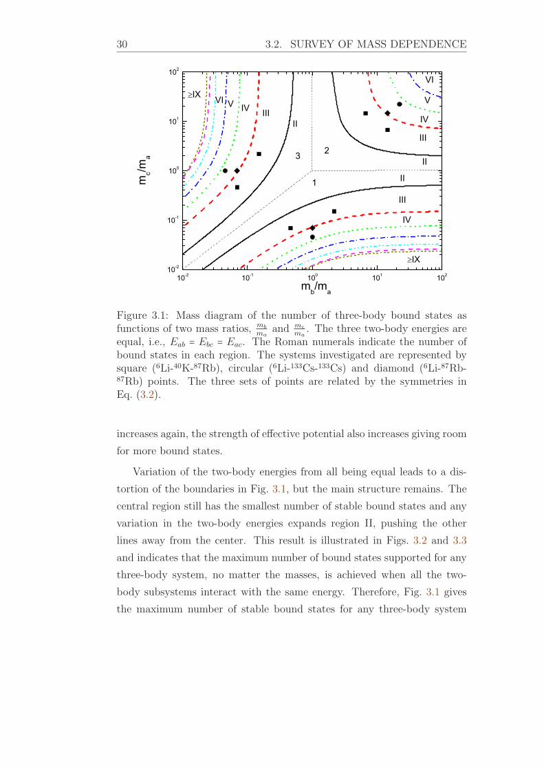
30 3.2. SURVEY OF MASS DEPENDENCE
10-2 10-1 100 101 10210-2
10-1
100
101
102
3 2
1
mb/ma
mc/m
a
IX
IX
II
II
II
III
III
III
IVIV
IV
VI
VI V V
Figure 3.1: Mass diagram of the number of three-body bound states asfunctions of two mass ratios, mb
maand mc
ma. The three two-body energies are
equal, i.e., Eab = Ebc = Eac. The Roman numerals indicate the number ofbound states in each region. The systems investigated are represented bysquare (6Li-40K-87Rb), circular (6Li-133Cs-133Cs) and diamond (6Li-87Rb-87Rb) points. The three sets of points are related by the symmetries inEq. (3.2).
increases again, the strength of effective potential also increases giving room
for more bound states.
Variation of the two-body energies from all being equal leads to a dis-
tortion of the boundaries in Fig. 3.1, but the main structure remains. The
central region still has the smallest number of stable bound states and any
variation in the two-body energies expands region II, pushing the other
lines away from the center. This result is illustrated in Figs. 3.2 and 3.3
and indicates that the maximum number of bound states supported for any
three-body system, no matter the masses, is achieved when all the two-
body subsystems interact with the same energy. Therefore, Fig. 3.1 gives
the maximum number of stable bound states for any three-body system

CHAPTER 3. UNIVERSAL 2D THREE-BODY BOUND STATES 31
composed for particles with different masses.
10-2 10-1 100 101 10210-2
10-1
100
101
102
mb/m
a
mc/m
a
VIII
III
II
Eab
=0 ; Eac
= Ebc
1
23 I
Figure 3.2: Mass diagram of the number of three-body bound states asfunctions of two mass ratios, mb
maand mc
ma. The two-body energies are Eab = 0
and Eac = Ebc. The Roman numerals indicate the number of bound statesin each region. The systems investigated are represented by square (6Li-40K-87Rb), circular (6Li-133Cs-133Cs) and diamond (6Li-87Rb-87Rb) points.The numbers 1,2,3 label three different sectors.
Although presenting the richest energy spectrum, the scenario of three
distinct two-body subsystems interacting with the same energy seems hard
to be implemented experimentally. However, it was recently reported in
Ref. [Repp 2013] that mixtures of 133Cs and 6Li were successfully trapped
with a diverging scattering length of the 133Cs-133Cs subsystem. A system
composed of two-heavy particles and a light one is described for instance
in the region where mc < ma and mc < mb. Besides, if two particles do not
interact in 2D, their energy can be set null. A mass diagram which includes
such situaion (the 133Cs133Cs6Li system is represented as circular points in
Figs. 3.1 to 3.3) is constructed taking Eab = 0 and keeping Eac = Ebc and is

32 3.2. SURVEY OF MASS DEPENDENCE
shown in Fig. 3.2. Region I emerges in the middle of the figure, pushing the
other lines away from the center. Excited states are only present in sector
1, where the two non-interacting particles are heavier than the third one
(this configuration is studied in detail in Chapter 4).
The symmetries in Eq. (3.2), which clearly appear in Fig. 3.1, can not
be seen in Fig. 3.2, but this does not mean that symmetry was broken.
This apparent contradiction comes from the way that the mass-diagram
is built. In sector 1 the light particle is mc, i.e., mc < ma and mc < mb,
so that Eab = 0 means that the two heaviest particles are not interacting.
Starting in sector 1 of Fig. 3.2 and moving towards sector 2, after crossing
the horizontal dashed line Eab = 0 does not mean that the two heaviest
particles are not interacting any more, since in this region the particles b and
c are the heaviest, i.e., ma < mb and ma < mc and the effective interaction
between the heavy particles is mediated by light one, namely particle a.
The same happens in region 3, where particles a and c are the heaviest. In
fact, a mass-diagram for imbalanced two-body energies shows information
for three different systems. Therefore, each sector in Fig. 3.2 obey the
symmetries in Eq. (3.2) itself. For instance, the configuration showed in
Fig. 3.2 is also described for Ebc = 0 with ma < mb and ma < mc or Eac = 0with mb < ma and mb < mc. These choices lead to two other plots, where
the boundary lines in Fig. 3.2 rotates to sector 2 and 3, respectively. Notice
that the symmetries in Eq. (3.2) are not well defined for a non-interacting
two-body subsystem, however, it is not hard to extend them for this case.
What about a system where all two-body energies are different from each
other? This scenario is shown in Fig. 3.3. In sector 1, where the energy
between the two heaviest particles is greater than the other ones, the three
distinct systems which are shown in Figs. 3.1 and 3.2 have only one bound
state each. In this energy-configuration, region 2 should be the most similar
to the previous case, where the heavy-heavy system is not as bound as the
other ones. However, sectors 2 and 3 seems to be almost symmetric in
Fig. 3.3, showing that both 6Li-133Cs-133Cs and 6Li-87Rb-87Rb systems have
two bound states each. A small difference is seem for 6Li-40K-87Rb, which

CHAPTER 3. UNIVERSAL 2D THREE-BODY BOUND STATES 33
10-2 10-1 100 101 10210-2
10-1
100
101
102
mc/m
a
mb/ma
3
1
2
I
I
IV
IV
III
III
III
I
II
II
Eab
=10 Eac
; Ebc
=0.1 Eac
Figure 3.3: Mass diagram of the number of three-body bound states asfunctions of two mass ratios, mb
maand mc
ma. The two-body energies are Eab =
10Eac and Ebc = 0.1Eac. The Roman numerals indicate the number ofbound states in each region. The systems investigated are represented bysquare (6Li-40K-87Rb), circular (6Li-133Cs-133Cs) and diamond (6Li-87Rb-87Rb) points. The numbers 1,2,3 label three different sectors.
has two bound states in sector 2, but only one in sector 3. The similarity
between sector 1 in Fig. 3.2 and sector 2 in Fig. 3.3 is not clear enough
because the strongly bound heavy-light system changes the threshold of
binding the three-body system, cutting-out the most weakly three-body
bound states. More details about these mass-diagrams and discussion about
bound states are found in [Bellotti 2011,Bellotti 2012,Bellotti 2013b].
3.3 Three-body energies for given masses
Realistic scenarios correspond to given particles (atoms or molecules) with
known masses where in contrast, the interactions are variable through Fes-
hbach resonances [Chin 2010]. Once the constituents are chosen, the di-

34 3.3. THREE-BODY ENERGIES FOR GIVEN MASSES
agrams from the last section can be powerful guides in the experimental
search for 2D three-body bound states, as they indicate how many bound
states are expected to exist. However, this number vary for different two-
body energies. The dependence in the number of bound states with the
two-body energies for a specific system is discussed in this section.
Assuming masses corresponding to the alkali atoms 87Rb, 40K and 6Li,
the two ratios of two-body energies are left as variables where each set
uniquely specifies the three-body energies of ground and possibly excited
states. A contour diagram of the scaled three-body energies for the two
lowest stable bound states of the chosen system is shown in Fig. 3.4. The
log-log plot can be deceiving and on a linear scale the curves of equal scaled
three-body energy would be concave for the ground state and almost linear
or slightly convex for the first excited state in contrast to the convex con-
tours in Fig. 3.4. The chosen set of masses only allow one, two, or three
stable bound states, depending on the two-body energies. The correspond-
ing regions are shown by dotted curves in Fig. 3.4. The true extent of the
regions cannot be seen. Both region II and III are closed, namely, region II
continues along region III up to energy ratios of about 10±5, and the narrow
region III is entirely embedded in region II. Other sets of mass ratios, as
6Li-133Cs-133Cs or 6Li-87Rb-87Rb, for instance, could open region III and
allow regions inside with more than three stable bound states.
In the log-log plot of Fig. 3.4 the two-body energies vary by five orders
of magnitude, whereas the scaled three-body energies for a stable system
must be larger than all two-body energies. The three-body energy contours
connect minimum and maximum two-body energies, that is zero and max-
imum two-body energies for the ground state and thresholds boundaries
for existence of the excited states [Bellotti 2011]. The contours appear in
regular intervals with larger values for increasing two-body energies. Large
three-body energies reflect small spatial extension and therefore are less
interesting as it presumably is unreachable in the universal limit. The con-
tours pass continuously through the boundaries of the different regions since
the ground state exists without knowledge of the excited states. The con-

CHAPTER 3. UNIVERSAL 2D THREE-BODY BOUND STATES 35
10-3 10-2 10-1 100 101 10210-3
10-2
10-1
100
101
102
I
I
IIIIIground
3=3
3=8
3=15
3=40
3=100
first
3=2
3=3
3=5
3=10
AC
BC
I
Figure 3.4: Contour diagrams with lines of fixed ǫ3 values as function of thetwo-body energies ǫac and ǫbc. The solid and dashed curves are for groundand excited states, respectively. Here a is 87Rb, b is 40K, and c is 6Li. Thedotted curves show where the number of stable bound states change fromone (regions most asymmetric for small energies), to two (comparable sizeof the two-body energies), and to three (equal and large energies). Theroman labels I, II, and III are as in Fig. 3.1.
tours in Fig. 3.4 for the excited state can only appear in the regions with two
or more stable bound states. These contours therefore must connect points
of the boundaries between regions I and II. They may cross continuously
through region III precisely as the ground state would cross through bound-
aries between regions I and II. Similar contours exist within region III but
are not exhibited in this narrow strip where they are allowed. The scaled
three-body energies are often substantially larger than the initial two-body
energies, although both arise from the same two-body interactions.

36 3.4. PARAMETRIZATION OF THREE-BODY ENERGIES
3.4 Parametrization of three-body energies
The universal functions Fn defined in Eq. (3.1) are not easily found. Their
dependence on masses and two-body energies are highly non-trivial, even in
a simpler scenario of two identical particles and a distinct one [Bellotti 2011].
However, the contour diagrams in Fig. 3.4 suggest a simple implicit depen-
dence in terms of an extended Lame curves or super ellipses [Lame 1818].
Note that, despite of the log-log scale in Fig. 3.4, the parametrization in
terms of Lame curves is done with the energies on a linear scale. The
three-body energies can be written indirectly by super circles, i.e.,
ǫtnac + ǫtnbc = Rtn
n , (3.3)
where the radius, Rn, and the power, tn, are functions of ǫ3 and both de-
pend on the two mass ratios. The term super circle has been adopted
since Eq. (3.3) only differs from a circumference of radii Rn and coordinates
(ǫac, ǫbc) in the power tn, which is not equal two in general. The smallest
value of ǫ3 is unity corresponding to the two-body threshold of the ab system
used as the energy unit.
Two sets of alkali atoms (6Li-40K-87Rb and 40K-87Rb-133Cs) and a system
of three identical particles are used to validate the parameterization. The
fitted radius and exponent functions are respectively shown in Figs. 3.5 and
3.6 for both ground and first excited states.
The radius functions turn out to be surprisingly simple, that is linear
functions of ǫ3, which are essentially independent of the masses. For the
ground state a slight increase of slope with increasing three-body energy is
found. Average estimates are
R0(ǫ3) ≈ 0.74ǫ3 − 2.5 , R1(ǫ3) ≈ ǫ3 . (3.4)
The increasing functions reflect how the contours in Fig. 3.4 are moving
to larger two-body energies with increasing ǫ3. This simple linear depen-
dence implies that the three-body energy increases linearly with a kind of

CHAPTER 3. UNIVERSAL 2D THREE-BODY BOUND STATES 37
average of the two two-body energy ratios. Notice that the symmetric sys-
tem, where all particles are identical, has this property where two- and
three-body energies are proportional in the universal limit. To approach
this limit it is assumed firstly that a = b, and Eqs. (3.3) and (3.4) imply for
the ground states that 0.74ǫ3 ≈ 2.5 + ǫac21/t0 . When a = b = c, the known ra-
tios ǫ3 ≈ (2.5 + 21/t0)/0.74 = 16.52 for the ground state and ǫ3 ≈ 21/t1 = 1.267for the excited state are recovered. This is achieved with t0 ≈ 0.30 and
t1 ≈ 2.93 and both t0 and t1 agree with the ones calculated in Fig. (3.6).
0 20 40 60 80 1000
20
40
60
80
100
Rn(
)
ground - R0( ) equal masses 6Li-40K-87Rb 40K-87Rb-133Cs
first - R1( ) (x10) equal masses 6Li-40K-87Rb 40K-87Rb-133Cs
Figure 3.5: The functions, R0 and R1, of the three-body energy ǫ3 in thesuper-ellipse fit for three sets of mass ratios, which are (mα,mβ) = (1,1),(40/87,6/87), (87/133,40/133) corresponding to three identical molecules,6Li-40K-87Rb, and 40K-87Rb-133Cs, respectively. Both axis are scaled up bya factor of 10 for the excited state, where the maximum energy of ǫ3 = 10corresponds to R1 ≈ 10.
The exponents tn are crucial to obtain the correct curvature of the energy
contours in Fig. 3.4. In Fig. 3.6 are shown the functions obtained by fitting
results for the same sets of masses as in Fig. 3.5. These exponents increase
monotonously with ǫ3 from small values and the curves bend over at some

38 3.4. PARAMETRIZATION OF THREE-BODY ENERGIES
point and continue to increase linearly with a smaller slope. Eventually the
curves would stop when the states reach a two-body threshold and become
unstable. In most cases this only happens for excited states at large energies
where the universal properties are, in practice, probably much more unlikely
to realize.
0 20 40 60 80 1000,15
0,20
0,25
0,30
0,35
0,40
0 20 40 60 80 1000
5
10
15
20
25
30
t 1()
t 0()
equal masses 6Li-40K-87Rb 40K-87Rb-133Cs
Figure 3.6: The exponents, t0 and t1, in the super-ellipse fit as func-tions of the three-body energy ǫ3 for three sets of mass ratios, which are(mα,mβ) = (1,1), (40/87,6/87) and (87/133,40/133) corresponding to iden-tical molecules, 6Li-40K-87Rb, and 40K-87Rb-133Cs, respectively.
The absolute sizes increase by about an order of magnitude from ground
to first excited state. As said before, the role of the exponents in Eq. (3.3)
is to adjust to the curvature of the contours in Fig. 3.4. Thus, large t is nec-
essary for strongly bending curves. This immediately explain the difference
between ground and first excited state, but also the overall increase with ǫ3.
This is especially pronounced for the excited states which are squeezed in
between boundaries defined by stability towards decay to bound two-body

CHAPTER 3. UNIVERSAL 2D THREE-BODY BOUND STATES 39
subsystems.
The behavior of the exponents is also surprisingly simple for each set
of masses. The relatively fast increase at small energies in Fig. 3.6 slows
down and both t0 and t1 approach constants at large energy. For the ground
state, this can be accurately captured by
t0(ǫ3) ≈ α0
ǫp03+ β0
ǫp03+ γ0
, (3.5)
where α0 is the mass dependent constant approached at large energy (see
Fig. 3.6). The parameters, (p0, α0) ≃ (0.04−0.06,0.3−0.5), exhibits a small
mass dependence, whereas (β0, γ0) ≃ −(0.93−0.95),−(0.82−0.87) are slightlynegative but almost mass independent. Remember that stability requires
ǫ3 > 1. The value of t0 for small ǫ3 ≈ 1 is then in the range of t0 ≃ 0.2−0.5 as
required to give the limiting value of ǫ3 = 16.52. A similar parametrization
for the exponent corresponding to the excited state can be found.
Combining Eqs. (3.3), (3.4) and (3.5), the parameterized results cannot
be distinguished from the computed curves in Fig. 3.4.


Chapter 4
Adiabatic approximation
Why does the number of bound states increase as one particle becomes
lighter than the other two? This question arises after looking the mass-
diagrams in Chapter 3, where an increasing number of bound states was
found for decreasing the mass of one of the particles. The situation where
one particle is much lighter than the other two is suitably handled in the
adiabatic approximation, namely the Born-Oppenheimer (BO) approxima-
tion.
The BO approximation considers a system composed of two heavy parti-
cles and a light one, where the terms heavy and light have relative meaning:
two particles are heavier than the third one. In this approximation the heavy
particles move very slowly while the light particle orbits around them. In
fact, for the BO approximation be valid it is enough to consider the kinetic
energy of the heavy particles is much smaller than the light particle one.
A successful implementation of the BO approximation is presented in
Ref. [Fonseca 1979], where the Efimov problem is solved in an analytic
model. It is shown that the Efimov effect is related to a long-range effective
force and it can occur even when the individual pair forces have zero range.
This is an example of how long-range forces can arise in the three-body prob-
lem in a way unpredictable by two-body intuition. The BO approximation
was also implemented in Ref. [Lim 1980], looking for the Efimov effect in
2D mass-imbalanced three-body systems, however the mass-dependence of
such systems was not addressed.
The BO approximation of 2D three-body systems is re-visited under the
mass-dependence perspective [Bellotti 2013b]. As in the previous Chapter,
a 2D three-body system with short-range interactions for general masses
41

42 4.1. ADIABATIC POTENTIAL
and interaction strengths is considered. The expressions for the adiabatic
approximation are derived using separable zero-range potentials and yield
a concise adiabatic potential between the two heavy particles in the heavy-
heavy-light system when the light particle coordinate is integrated out.
The adiabatic potential, which is found as the solution of a transcenden-
tal equation, is mass-dependent and reveals an increasing number of bound
states by decreasing the mass of the light. An asymptotic expression for
the adiabatic potential is derived and it is shown that this analytic expres-
sion faithfully corresponds to the numerically calculated adiabatic poten-
tial, even in the non-asymptotic region. The number of bound states for a
heavy-heavy-light system is estimated as a function of the light-heavy mass
ratio. Infinitely many bound states are expected as this ratio approaches
zero. However, for finite masses a finite number of bound states is always
expected.
4.1 Adiabatic potential
An abc system where the two heavy particles have masses ma and mb is
considered. These particles are fixed and their centers are separated out by
a distance R. The light particle has mass mc and coordinate r relative to
the CM of the heavy-heavy subsystem. The interaction between particles
is described by zero-range pairwise potentials. The notation for the poten-
tial is that vc means the interaction between particles a and b, with va, vb
analogously defined. The configuration of the three-body system is shown
in Fig. 4.1.
The Schrodinger eigenvalue equation of the abc system is HΨ(r,R) =EΨ(r,R). The Hamiltonian H is written in the relative coordinates R, r
in the three-body CM frame as
H = − h2
2mab
∇2
R −h2
2mab,c
∇2
r + va (r − mab
mb
R) + vb (r + mab
ma
R) + vc(R),(4.1)

CHAPTER 4. ADIABATIC APPROXIMATION 43
Figure 4.1: Three-body relative coordinates used in the adiabatic approxi-mation.
where the reduced masses are mab = mamb/(ma +mb) and mab,c = mc(ma +
mb)/(ma +mb +mc).The adiabatic approximation says that it is possible to split the three-
body eigenvalue equation into the solution of two two-body problems: the
light particle motion is considered with respect to the heavy-heavy system
and the heavy-heavy system motion is separated out. These eigenvalue
equations are valid whenever the motion of the light particle is rapid com-
pared to the motion of the heavy ones, so that the light particle dynamics
can be solved while the heavy particles are instantaneously at rest. The
wave function is decomposed as
Ψ(r,R) = ψ(r,R)φ(R) , (4.2)
where ψ(r,R) is the wave function describing the state of the light particle
for fixed R and φ(R) is the heavy subsystem wave function. The approx-
imation is valid when the kinetic energy term, − h2
2mab∇
2
Rψ(r,R), is small
compared to the other terms in Eq.(4.1). Using the wave function from

44 4.1. ADIABATIC POTENTIAL
Eq. (4.2), the eigenvalue equation becomes
Hψ(r,R)φ(R) = Eψ(r,R)φ(R) ,φ(R)(− h2
2mab,c
∇2
r + va (r − mab
mb
R) + vb (r + mab
ma
R))ψ(r,R)+ ψ(r,R) (− h2
2mab
∇2
R + vc(R))φ(R) = Eψ(r,R)φ(R) ,(− h2
2mab,c∇2
r + va (r − mab
mbR) + vb (r + mab
maR))ψ(r,R)
ψ(r,R)+
(− h2
2mab∇
2
R + vc(R))φ(R)φ(R) = E . (4.3)
The first term on the left-hand-side of Eq. (4.3) is a separation constant,
ǫ(R), which does not depend on r. Therefore, light particle equation is
[− h2
2mab,c
∇2
r + va (r − mab
mb
R) + vb (r + mab
ma
R)]ψ(r,R) = ǫ(R)ψ(r,R) ,(4.4)
and the eigenvalue, ǫ(R), plays the role of an effective potential in the
equation for the heavy-heavy system. From Eq. (4.3), this equation is
(− h2
2mab
∇2
R + vc(R) + ǫ(R))φ(R) = Eφ(R) . (4.5)
Assuming that the potentials in Eq.(4.4) are separable and have the
same strength, i.e., vα = λ ∣χα⟩ ⟨χα∣, the wave function of the light particle
in momentum space reads
ψ(p) = λ g(p)ǫ(R) − h2
2mab,cp2[eımab
ma
p⋅R
h A+ + e−ımabmb
p⋅R
h A−] , (4.6)
where
A± = ∫ d2r′g† (r′ ± mab
ma
R)Ψ (r′) = ∫ d2p′g† (p′) e∓ımabma
p′⋅R
h
2πψ (p′) (4.7)

CHAPTER 4. ADIABATIC APPROXIMATION 45
and g(p) is the form factor of the potential.
The formulation of Eq. (4.6) in terms of A± leads to the system of equa-
tions
A± = λ∫ d2p∣g(p)∣2
ǫ(R) − h2
2mab,cp2(e∓ıp⋅Rh A∓ +A±) . (4.8)
The non-trivial solution of Eq.(4.8), i.e., A± ≠ 0, gives a transcendental
equation for the effective potential, which reads
1
λ= ∫ d2p
∣g(p)∣2ǫ(R) − h2
2mab,cp2[1 + cos(p ⋅R
h)] . (4.9)
Using the binding energy of the heavy-light subsystem, E2, to parameterize
λ [Adhikari 1995a], Eq. (4.9) is rewritten as
∫ d2p∣g(p)∣2 ⎡⎢⎢⎢⎢⎣1 + cos(p⋅R
h)
ǫ(R) − h2
2mab,cp2+
1∣E2∣ + h2
2mab,cp2
⎤⎥⎥⎥⎥⎦ = 0 . (4.10)
Model-independent results are naturally obtained with the use of zero-
range potentials and the form factor of such potential in momentum space is
a constant, i.e., g(p) = 1. In this case, Eq. (4.10) is finite and the integration
of the two terms leads to the transcendental equation for the adiabatic
potential
ln∣ǫ(R)∣∣E2∣ = 2K0
⎛⎝√
2mab,c∣ǫ(R)∣h2
R⎞⎠ , (4.11)
where K0 is the modified Bessel function of second kind of order zero.
The effective potential ǫ(R) is exactly defined as the solution of Eq. (4.11)
and is a powerful tool in understanding mass-imbalanced three-body sys-
tems in two dimensions. However, a transcendental equation involving a
logarithm and a modified Bessel function of second kind is not intuitive at
all. In the next section, two limiting expressions are found by expanding
both sides of Eq. (4.11) for small and large R.

46 4.2. ASYMPTOTIC EXPRESSIONS
4.2 Asymptotic expressions
The asymptotic form for ∣R∣ → 0 is found inserting the asymptotic form of
K0 for small arguments [Abramowitz 1965] into Eq. (4.11). The result is a
Coulomb-like potential, which up to 2nd order reads
∣ǫasymptotic(R)∣∣E2∣ → 2e−γs(R) (1 − e
−γ2s(R) [(1 − γ) − 1
2ln(e−γ
2s(R))])−1 ,
(4.12)
where γ is the constant of Euler and s(R) =√2mab,c∣E2∣h2 R.
When the distance R between the two heavy particles is large, i.e.,
∣R∣ →∞, the light particle feels only the interaction from one of the heavy
particles. In this limit the three-body problem becomes a two-body problem
and is expected that ∣E∣ = ∣E2∣. Therefore, defining ∣ǫ(R)∣∣E2∣ = 1 + V (R), thiscondition is fulfilled when V → 0 for ∣R∣ → ∞. Replacing ∣E∣ / ∣E2∣ by1 + V (R) in Eq. (4.11) and expanding both sides up to first order in R
results in
V (R) = 2K0 (s(R))1 + s(R) K1 (s(R)) , (4.13)
The asymptotic expression of the adiabatic potential for large R is then
∣ǫasymptotic(R)∣∣E2∣ → 1 +2K0 (s(R))
1 + s(R) K1 (s(R)) → 1 +√2π
e−s(R)√s(R) . (4.14)
Notice that the approximation accuracy increases when higher order
terms are included in the expansions. It is possible to go to more pre-
cise adiabatic potential representations taken higher order expansions of
Eq. (4.11). However, the results of the approximations (4.12) and (4.14)
and the adiabatic potential (4.11) are almost indistinguishable in practice.
The largest deviations, shown in Fig. 4.2, are found in the region 0.3 < s < 3,where the difference between ǫasymptotic(s) and ǫexact(s) never exceeds 9%.
In spite of the fact that the asymptotic potential in Eqs. (4.12) and
(4.14) is valid respectively in the extreme limits R → 0 and R → ∞, it
perfectly reproduces the effective potential in almost all the range of the

CHAPTER 4. ADIABATIC APPROXIMATION 47
10-3 10-2 10-1 100 101 102
0.92
0.96
1.00
1.04asymptotic(s)
s s 0 (1st order) s 0 (2nd order)
asym
ptotic(s)/
exac
t(s)
s
Figure 4.2: Ratio ǫasymptotic(s)/ǫexact(s) as function of the dimensionless co-ordinate s, showing the validity of asymptotic expressions in Eqs. (4.12) and(4.14). The black-solid and red-dashed curves are the first order expansionof the adiabatic potential at small and large distances, respectively. Thegreen-dotted curve is the second order expansion of the adiabatic potentialat small distances.
scaled coordinate s(R), since its difference to the potential numerically
calculated from Eq. (4.11) is almost imperceptible. These features are shown
in Fig.4.3.
For R → 0 the first order expansion of the effective potential in Eq. (4.12)
resembles a hydrogen atom in 2D, where the pre-factor 1/√mc makes the
energy of the deepest states grow without boundaries when mc → 0. Fur-
thermore, for R →∞, the potential in Eq. (4.14) is long-ranged and screened
by a factor√mc, which becomes less important for mc → 0. Therefore, an
increasing number of bound states is expected when particle c is much lighter
than the other ones, i.e., mc → 0, since the adiabatic potential becomes more
attractive and less screened in this limit. Still, these states will accumulate
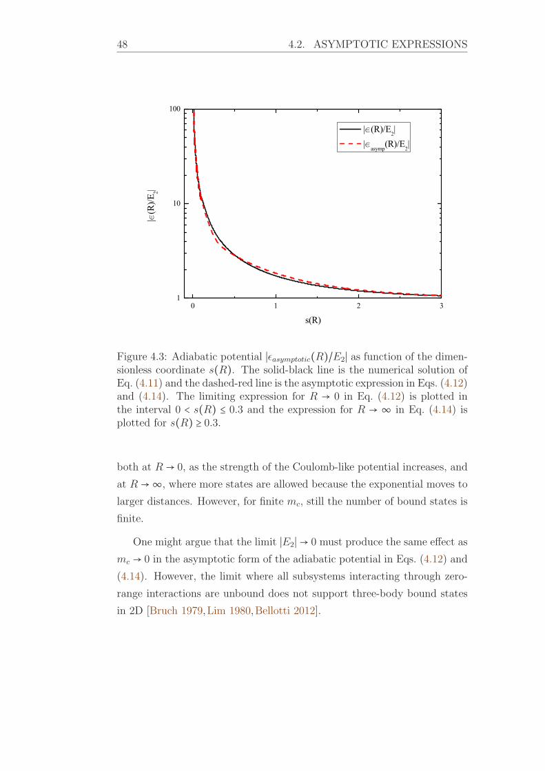
48 4.2. ASYMPTOTIC EXPRESSIONS
� � � ��
��
���
��������
���
���������
���� ������
��
Figure 4.3: Adiabatic potential ∣ǫasymptotic(R)/E2∣ as function of the dimen-sionless coordinate s(R). The solid-black line is the numerical solution ofEq. (4.11) and the dashed-red line is the asymptotic expression in Eqs. (4.12)and (4.14). The limiting expression for R → 0 in Eq. (4.12) is plotted inthe interval 0 < s(R) ≤ 0.3 and the expression for R → ∞ in Eq. (4.14) isplotted for s(R) ≥ 0.3.
both at R → 0, as the strength of the Coulomb-like potential increases, and
at R →∞, where more states are allowed because the exponential moves to
larger distances. However, for finite mc, still the number of bound states is
finite.
One might argue that the limit ∣E2∣→ 0 must produce the same effect as
mc → 0 in the asymptotic form of the adiabatic potential in Eqs. (4.12) and
(4.14). However, the limit where all subsystems interacting through zero-
range interactions are unbound does not support three-body bound states
in 2D [Bruch 1979,Lim 1980,Bellotti 2012].

CHAPTER 4. ADIABATIC APPROXIMATION 49
4.3 Numerical results
The increasing number of three-body bound states as function of the mass of
the particles, presented in Chapter 3, was qualitatively explained in the last
section with the asymptotic expressions of the adiabatic potential. In this
section, the analytic properties of the asymptotic expressions in Eqs. (4.12)
and (4.14) are used in the numerical survey of bound states in the adiabatic
limit.
In the following, the analysis is done for a system of two identical heavy
particles of masses ma = mb =M in units that h2 =M = Eac = Ebc = E2 = 1.The mass ratio between light and heavy particles is defined m = mc
M. In this
case, the reduced mass mab,c is written as
mab,c = 2m
m + 2and mab,c →m for m→ 0 . (4.15)
With these units, the asymptotic expression for the effective potential be-
comes
ǫ(R)→ − 2e−γ√4mm+2 R
⎛⎝1 − e−γ2
√4m
m + 2R
⎡⎢⎢⎢⎢⎣(1 − γ) −1
2ln⎛⎝e−γ2
√4m
m + 2R⎞⎠⎤⎥⎥⎥⎥⎦⎞⎠−1,
(4.16)
for√
4mm+2 R ≤ 1.15 and
ǫ(R)→ −1 −√2π e−√
4mm+2
R√(√ 4m
m+2)1
2
R
, (4.17)
for√
4mm+2R ≥ 1.15. Notice that this approximation is very accurate even
when 2R ≈ 1.15√(1 + 2/m) where the largest deviation of 9% is reached.
The Schrodinger equation for the heavy-heavy system in Eq. (4.5) is
transformed in a Sturm-Liouville eigenvalue equation in a Lz = 0 state. The

50 4.3. NUMERICAL RESULTS
wave function φ(R) is replaced by χ(R)√R
giving
[−( d2dR2+
1
4R2) + vc(R) + ǫ (R)]χ(R) = E3 χ(R) , (4.18)
where E3 is the three-body energy and ǫ (R) is given in Eqs. (4.16) and
(4.17). Genuinely bound states are present when E3−E2 ≤ 0, or equivalently∣E3∣ ≥ ∣E2∣, since bound states have negative energies.
The differential equation (4.18) is numerically solved to estimate the
number of bound states (NB) for a system with mass ratiom when the heavy
particles do not interact with each other. Due to the attractive centrifugal
barrier in 2D, all the two-body subsystems interact with finite energy. This
means that Eab = 0 implies in a non-interacting ab subsystem. Once the
heavy-heavy is not interacting, Eab = 0 is translated to vc = 0 in Eq. (4.18).
If vc is attractive and able to support bound states, the three-body system
would effectively be reduced to the lightest particle moving around a heavy-
heavy dimer. The corresponding additional much deeper-lying bound states
are, however, not interesting in the present context.
The method to solve Eq. (4.18) numerically consists in writing this eigen-
value equation in matrix form. The operators, potential, wave function and
the radial coordinate in this equation are discretized, which leads to a tridi-
agonal matrix form. This tridiagonal matrix is then diagonalized to give
the eigenvalues of the problem. It is also possible to calculate the number
of bound states (NB) by solving the set of homogeneous integral equations
(2.68).
Counting the number of bound states, a critical mass ratio (mt) is intro-
duced, above which NB bound states are available. These critical values are
shown in Fig. 4.4, where a comparison between the solutions of the differ-
ential equation (4.18) and homogeneous coupled integral equations (2.68) is
made.
The results in Fig. 4.4 show that the adiabatic approximation picks up
the small mass behavior very well, even for mass ratios up towards 1. There
is a small error in the threshold for the number of available bound states

CHAPTER 4. ADIABATIC APPROXIMATION 51
10-5 10-4 10-3 10-2 10-1 100
0
20
40
60
80
100
120
140
160
10-2 10-1
2
4
6
8
10
12
14
NB
m
Adiabatic approximation Integral equation
Figure 4.4: Number of possible bound states (NB) for a system with masses(1,1,m) and Eab = 0. The (black) squares represent the mass ratio m fromwhere NB states are bound, calculated through the adiabatic approxima-tion (4.18). The (red) circles represent the solutions of the set of coupledhomogeneous integral equations (2.68).
for 0 ≤ NB ≤ 14, but it decreases as m → 0. The adiabatic approximation
has an accuracy better than 10% for m = 0.01, as it can be seen in the
inset of Fig. 4.4. Due to the numerical difficulties, it is very hard to count
the number of bound states for NB > 14 by solving the set of coupled
homogeneous integral equation (2.68). Fortunately, it is very easy to do it
with the differential equation (4.18). It is clearly possible to see in Fig. 4.4,
that NB →∞ for m→ 0 as it was pointed out in the last section.
4.4 Estimate of the number of bound states
A fit to the results presented in Fig. 4.4 shows that the dependence of the
number of bound states, NB, with the mass ratio, m, is rather well described

52 4.4. ESTIMATE OF THE NUMBER OF BOUND STATES
by
NB ≈ 0.731√m
. (4.19)
This behavior can be explained by the old quantum mechanics. An usual
way to estimate the number of bound states in a semi-classical approxima-
tion of the one-dimensional quantum problem is
∫ p dq = Nπh . (4.20)
Taking into account the effective potential in Eq.(4.18) and proper units,
the number of bound states with energy up to E3 = 0 is estimated as
N = 1
π√2m∫∞
0
dx
√m
2x2− V (x) = 0.733√
m, (4.21)
where V (x) is the adiabatic potential (4.16) and (4.17) with x = √ 4mm+2R.
One could argue that the integral in Eq.(4.21) diverges in both limits and
can not be performed. Introducing a lower and an upper cut-off in the
integral, which are the same used in the numerical calculation (10−2 and
105 respectively), the result is N = 0.766√m. This result approaches the esti-
mative given in Eq. (4.19) as the diverging term on Eq.(4.21) becomes less
important when m becomes smaller. The integral in Eq.(4.21) is practically
m−independent for m ≤ 0.001 with the 10−2 cut-off, implying that the term
m/x2 is negligibly small by itself. The apparent divergences are due to the
semi-classical estimate, and accurately removed by cut-off at both small and
large x. The true quantum mechanical number of states are then recovered.
The estimate of the number of bound states in (4.19) and (4.21) nicely
agree. Besides that, this estimative is less than the upper limit for a two-
dimensional system with total angular momentum equal to zero, which is
given in [Khuri 2002]. For the adiabatic potential (4.16) and (4.17), this
upper limit is given by N = 0.5m. The difference between both estimates is
shown in Fig. 4.5. It was shown in Chapter 3 that any three-body system in
two dimensions will achieve its maximum number of bound states when all
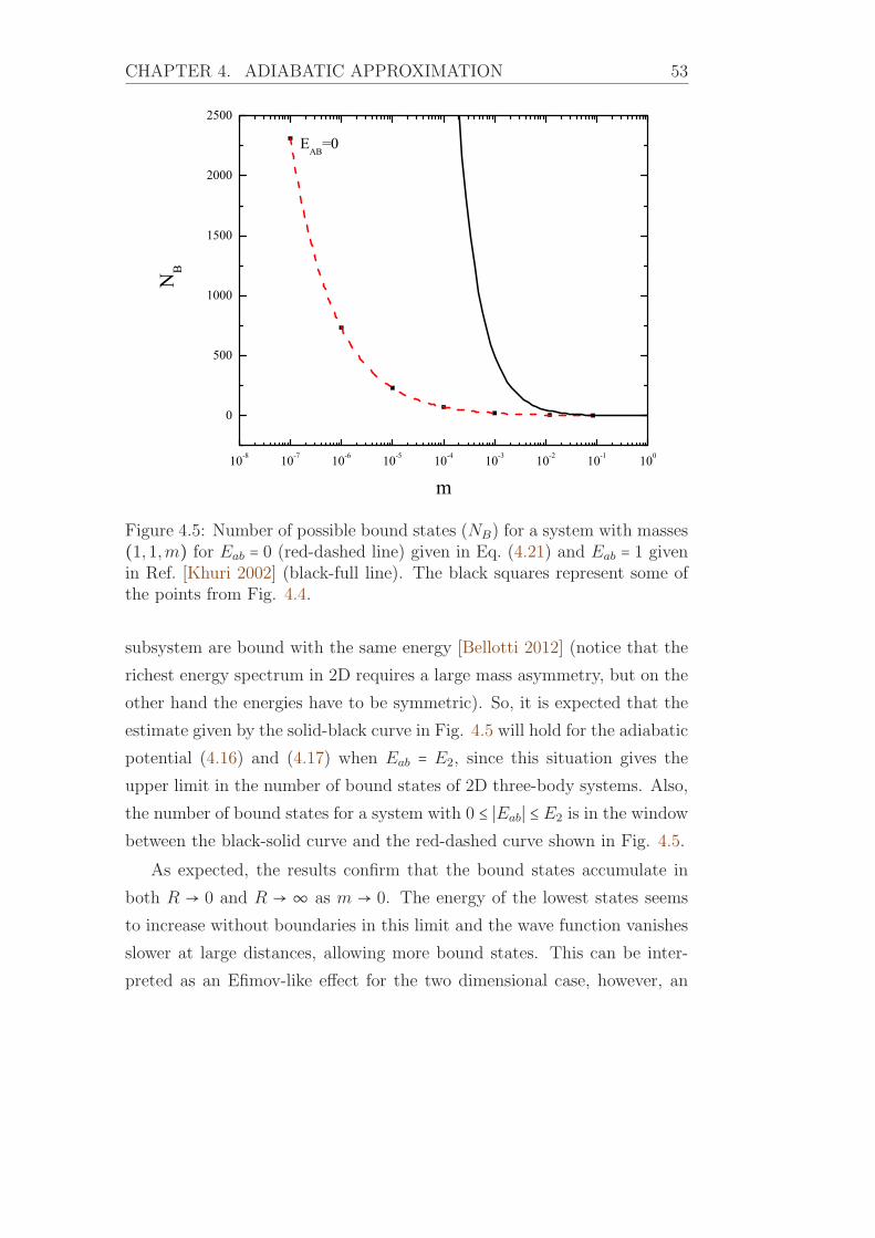
CHAPTER 4. ADIABATIC APPROXIMATION 53
10-8 10-7 10-6 10-5 10-4 10-3 10-2 10-1 100
0
500
1000
1500
2000
2500
EAB=0
NB
m
Figure 4.5: Number of possible bound states (NB) for a system with masses(1,1,m) for Eab = 0 (red-dashed line) given in Eq. (4.21) and Eab = 1 givenin Ref. [Khuri 2002] (black-full line). The black squares represent some ofthe points from Fig. 4.4.
subsystem are bound with the same energy [Bellotti 2012] (notice that the
richest energy spectrum in 2D requires a large mass asymmetry, but on the
other hand the energies have to be symmetric). So, it is expected that the
estimate given by the solid-black curve in Fig. 4.5 will hold for the adiabatic
potential (4.16) and (4.17) when Eab = E2, since this situation gives the
upper limit in the number of bound states of 2D three-body systems. Also,
the number of bound states for a system with 0 ≤ ∣Eab∣ ≤ E2 is in the window
between the black-solid curve and the red-dashed curve shown in Fig. 4.5.
As expected, the results confirm that the bound states accumulate in
both R → 0 and R → ∞ as m → 0. The energy of the lowest states seems
to increase without boundaries in this limit and the wave function vanishes
slower at large distances, allowing more bound states. This can be inter-
preted as an Efimov-like effect for the two dimensional case, however, an

54 4.4. ESTIMATE OF THE NUMBER OF BOUND STATES
important distinction between the 2D and 3D case must be done. While
the Efimov effect says that three identical particles can have infinitely many
bound states when E2 → 0, in 2D this limit leads to an unbound three-body
system. Infinitely many bound states are only expected in 2D when m = 0.Therefore, finite mc leads to a finite number of bound states.

Chapter 5
Momentum distribution in 2D
Another important theoretical prediction for cold atomic systems, which
was reported in Ref. [Tan 2008], is a parameter that emerges in the study
of two-component Fermi gases. This parameter, which is often called Tan’s
contact or two-body contact parameter and represented by C2, connects
universal two-body correlations and many-body properties. For instance,
the variation in the energy of a two-component Fermi gas of momentum kF
with the interaction strength (scattering length a) is directly proportional
to this parameter [Tan 2008], as it can be seen in
2πdE
d [−1/(kFa)] = C2 . (5.1)
Furthermore, the virial theorem for this atomic gas also relates with C2
through
E − 2V = − C2
4πkFa. (5.2)
These relations were confirmed in experiments with two-component Fermi
gases [Kuhnle 2010], where each side of Eqs. (5.1) and (5.2) were measured
independently and after compared to each other. A later experiment showed
that these relations also hold for bosons [Wild 2012].
The quantities in the left-hand-side of Eqs. (5.1) and (5.2) are defined
through the many-body properties of the gas, while the contact parameter
is defined in the few-body sector. A way to determine this parameter is to
find the coefficient in the leading order of the asymptotic one-body large
momentum density (n(q)) of few-body systems, namely
limq→∞n(q)→ C2
q4+C3F (q) . (5.3)
55

56
The next order in this expansion defines the three-body contact parame-
ter, C3, which may be important only for bosonic systems, since the Pauli
principle suppresses the short-range correlations for two-component Fermi
gases. Notice that the momentum dependence of the leading order term
in this expansion is the same for 1D, 2D and 3D systems [Valiente 2012],
but the function F (q), which is strongly related to the spectator functions,
depends on the the dimensionality of the system [Bellotti 2013a].
The spectator functions are the key ingredients for understanding the
asymptotic one-body momentum densities of few-body systems. While the
large momentum asymptotic behavior of such functions is well-known for
3D systems [Danilov 1961], a striking result presented in this Chapter is the
derivation of asymptotic expressions for the spectator functions of three-
distinguishable bosons in 2D [Bellotti 2013a,Bellotti 2014]. Using the ex-
pression for the large momentum behavior, this asymptotic equation is ex-
tended to the full range of the momentum and used to calculate an analytic
expression for C2 in the ground state.
For three identical bosons, the two-body contact parameter is found to
be a universal constant, in the sense that C2
E3is the same for both states, each
one described for a three-body energy E3 [Bellotti 2013a]. Furthermore,
the three-body contact parameter has a very different behavior in 2D, when
compared to 3D systems (the 3D system is discussed in Chapter 6).
It was showed in Chapters 3 and 4 that, in 2D, mixed-species systems
have a richer energy spectrum than symmetric mass systems. So, it is
important to understand how the asymptotic one-body momentum density
changes when dealing with mixed-species systems in 2D. In this case, C2 is
not a universal constant anymore, however the universality is recovered in at
least one special case of a three-body system composed for two identical non-
interacting particles. The sub-leading order in the asymptotic momentum
density presents the same functional form for both equal masses and mixed-
species systems [Bellotti 2014].

CHAPTER 5. MOMENTUM DISTRIBUTION IN 2D 57
5.1 Asymptotic spectator function
Exhaustive numerical analysis of the spectator function in Eq. (2.70) for
three-identical bosons strongly suggests that the large momentum asymp-
totic behavior of such functions is given by
limq→∞f(q)→ Γ
ln q
q2, (5.4)
where Γ is a constant of normalization, as it can be seen in Fig. 5.1.
101 102 103 104 105 10610-10
10-9
10-8
10-7
10-6
10-5
10-4
10-3
10-2
10-1
100
2
qE
f(q)
Figure 5.1: Spectator function, f(q), for the ground state calculated nu-merically (black solid line) and using the ansatz f(q) = A0
ln q
q2(red dashed
line). The solid (black) line tends to oscillates around the dashed (red) oneas q →∞ due to finite numerical precision.
The ansatz in Eq. (5.4) are, in fact, the exact large momentum asymp-
totic expression of the spectator function, even for mass-imbalanced systems
(within a constant). A system composed of three-distinguishable particles,

58 5.1. ASYMPTOTIC SPECTATOR FUNCTION
when all pairs are bound, have three distinct spectator functions in the
wave function expressed by Eq. (2.67) . However, their large-momentum
asymptotic behavior all remain identical, except for individual proportion-
ality factors. To prove that, Eq.(2.70) is rewritten as
fα (q) = 2πτα(q,E3)⎡⎢⎢⎢⎢⎢⎢⎢⎢⎢⎢⎣∫∞
0
dkkfβ (k)
(−E3 +q2
2mαγ+
k2
2mβγ)¿ÁÁÀ1 −
k2q2/m2γ
(−E3+ q2
2mαγ+ k2
2mβγ)2+
+∫∞
0
dkkfγ (k)
(−E3 +q2
2mαβ+
k2
2mβγ)¿ÁÁÀ1 −
k2q2/m2
β
(−E3+ q2
2mαβ+ k2
2mβγ)2
⎤⎥⎥⎥⎥⎥⎥⎥⎥⎥⎥⎦, (5.5)
with
τα(q,E3) =⎡⎢⎢⎢⎢⎢⎢⎣4πmβγ ln
⎛⎜⎜⎝¿ÁÁÁÀ q2
2mβγ,α−E3
Eβγ
⎞⎟⎟⎠⎤⎥⎥⎥⎥⎥⎥⎦
−1, (5.6)
where mβγ,α = mα(mβ +mγ)/(mα +mβ +mγ) and mβγ = (mβ +mγ)/(mβ +
mγ) are reduced masses, Eβγ the two-body energy and (α,β, γ) are cyclic
permutations of the particle labels (a, b, c). The two terms on the right-
hand-side of Eq.(5.5) have the same form, and one can be obtained from
the other by interchanging labels β and γ. Therefore it suffices to calculate
the first integral in Eq.(5.5).
The contribution for large q can, in principle, be collected from k-values
ranging from zero to infinity. Separating small and large k-contributions,
the integration is divided into two intervals, that is from zero to a large (q-
independent) momentum Λ≫√E3, and from Λ to infinity. Thus, Eq. (5.5)

CHAPTER 5. MOMENTUM DISTRIBUTION IN 2D 59
reads
fα (q) = τα(q,E3)⎡⎢⎢⎢⎢⎢⎢⎢⎢⎢⎢⎣∫
Λ
0
dkkfβ (k)
(E3 +q2
2mαγ+
k2
2mβγ)¿ÁÁÀ1 −
k2q2/m2γ
(E3+ q2
2mαγ+ k2
2mβγ)2+
+∫∞
Λ
dkkfβ (k)
( q2
2mαγ+
k2
2mβγ)¿ÁÁÀ1 −
k2q2/m2γ
(E3+ q2
2mαγ+ k2
2mβγ)2+ ...
⎤⎥⎥⎥⎥⎥⎥⎥⎥⎥⎥⎦, (5.7)
where the dots indicate that the second term in Eq.(5.5) should be added.
For q → ∞ the first term, fα,1, on the right-hand-side of Eq.(5.7) goes
to zero as
limq→∞fα,1 (q)→ mαγ/mβγ
q2 ln(q) ∫Λ
0
dkkfβ (k)¿ÁÁÀ1 −
k2q2/m2γ
(E3+ q2
2mαγ+ k2
2mβγ)2, (5.8)
where limq→∞ τα(q,E3) → [2mβγ ln q]−1, and both E3 and k2
2mβγare much
smaller than q2
2mαγ. The integral in Eq. (5.8) is finite and only weakly
q−dependent for large q ≫ Λ.
The asymptotic spectator function in Eq.(5.4) can be inserted in the sec-
ond term on the right-hand-side of Eq.(5.7), fα,2, because in the asymptotic
limit k > Λ. In the limit of large momentum, i.e., q →∞, fα,2 is
limq→∞fα,2 (q)→ Γβ
2mβγ ln q∫∞
Λ
dklnk
k ( q2
2mαγ+
k2
2mβγ)¿ÁÁÀ1 −
k2q2/m2γ
(E3+ q2
2mαγ+ k2
2mβγ)2,
→ Γβ
q2 ln q ∫∞
Λ/q dyln y + ln q
y (mβγ
mαγ+ y2) , (5.9)
with k = qy in the last expression. Carrying out the two integrals in Eq. (5.9)

60 5.1. ASYMPTOTIC SPECTATOR FUNCTION
results in
∫∞
Λ/q dyln y
y (mβγ
mαγ+ y2) =
1
2
ln2 y(mβγ
mαγ+ y2)
RRRRRRRRRRR∞
Λ/q+∫
∞Λ/q dy
y ln2 y
(mβγ
mαγ+ y2)2
→ − mαγ
2mβγ
ln2 (Λq)→ − ln2 q
2mβγ
mαγ
, (5.10)
∫∞
Λ/q dy1
y (mβγ
mαγ+ y2) =
ln y(mβγ
mαγ+ y2)
RRRRRRRRRRR∞
Λ/q+ 2∫
∞Λ/q dy
y ln y
(mβγ
mαγ+ y2)2
→ −mαγ
mβγ
ln(Λq)→ ln q
mβγ
mαγ
, (5.11)
where it is assumed that the integrals in the right-hand-side of Eqs. (5.10)
and (5.11) are finite and their contributions can be neglected when q →∞in comparison with the terms carrying the log’s.
Inserting Eqs. (5.10) and (5.11) in Eq.(5.9), the asymptotic expression
of fα,2 reads
limq→∞fα,2 (q)→ Γβ
q2 ln q ∫∞
Λ/q dyln y + ln q
y (mβγ
mαγ+ y2) ,
→ Γβ
q2 ln q(− mαγ
2mβγ
ln2 q + ln qmαγ
mβγ
ln q) ,→ mαγ
mβγ
Γβ
ln q
q2. (5.12)
The missing term from Eq. (5.5) is recovered by interchanging the labels
γ by β in Eq.(5.12). The large-momentum behavior of the spectator function
is therefore
limq→∞fα (q)→ ( mαγ
2mβγ
Γβ +mαβ
2mβγ
Γγ) ln qq2
. (5.13)
Replacing fα(qα) in Eq. (5.13) by its conjectured asymptotic form, Eq. (5.4),
results in a system of three linear equations for the three unknown, Γα =mαγ
2mβγΓβ +
mαβ
2mβγΓγ, which can be rewritten as mβγΓα = mαγΓβ = mαβΓγ.
The large-momentum asymptotic behavior for the three distinct spectator

CHAPTER 5. MOMENTUM DISTRIBUTION IN 2D 61
functions are then
limq→∞fα(q)→ Γ
mβγ
ln q
q2. (5.14)
This result relates the asymptotic behavior of the three spectator functions
for any state. The remaining constant Γ still depends on which excited state
is considered, and also on two-body masses, energies and normalization.
101 102 103 104 105 106-2.0x10⁻⁶
-1.0x10⁻⁶
0.0
1.0x10⁻⁶
2.0x10-6
=6Li , = 133Cs = 133Cs , = 6Li =
f(q
)-/m
ln(q
)/q2
q / (m E )1/2
Figure 5.2: The difference fα (q) − Γ
mβγ
ln q
q2as a function of the momentum
q. The solid (black) and dash (red) lines are respectively the spectatorfunction of 6Li and 133Cs in a 133Cs-133Cs-6Li system. The dot (green) lineis the spectator function of a system composed for three identical bosons.Notice that Eq. (5.14) exactly describes the asymptotic spectator function,up to the numerical accuracy.
The derived large momentum asymptotic expression and the coefficients
in Eq.(5.14) beautifully agree with the numerical calculation. In Fig. 5.2,
the difference fα (q) − Γ
mβγ
ln q
q2is plotted as function of the momentum q
for the two different spectator functions in the 133Cs133Cs6Li system. The
same difference for a three-body system composed of identical bosons is also

62 5.1. ASYMPTOTIC SPECTATOR FUNCTION
shown. The nice agreement between the analytic derivation and the numer-
ical calculation demonstrate that the large momentum asymptotic behavior
is always ln q/q2 for any spectator function in 2D three-body systems.
101 102 103 104 1051.0
1.1
1.2
1.3
1.4
1.5
1.6
1.7
1.8
1.9
2.0f i(q
) / f j(q
)
q / (m EC)1/2
fA(q) / f
B(q)
fA(q) / f
C(q)
fB(q) / f
C(q)
Figure 5.3: Ratios between the three distinct spectator function for a genericcase of three distinct particles. Discrete points are the ratios between spec-tator functions numerically calculated from Eq. (2.70) and full lines areratios between coefficients in Eq.(5.14).
The general behavior of the large-momentum asymptotic form of the
spectator function is further demonstrated in Fig. 5.3 for a system of three
distinct particles. The numerically calculated points are compared to the
full lines obtained from Eq. (5.14). This comparison is again consistent
with the derived asymptotic behavior, and furthermore exhibit the rate
and accuracy of the convergence. The limit is reached within 10% and 1%
already for q ≈ 50 and q ≈ 104, respectively.
CHAPTER 5. MOMENTUM DISTRIBUTION IN 2D 63
5.1.1 Parameterizing from small to large momenta
The asymptotic spectator function in Eq. (5.14) seems to be a good approx-
imation even for moderate values of q, e.g., q ≈ 3√E3. Information about
the large-distance behavior for a given binding energy is also available, that
is exp(−κρ), where κ is related to the binding energy and ρ is the hyper-
radius. Fourier transformation then relates to the small momentum limit
with an overall behavior of (D + q2)−1, where D is a constant related to the
energy. This perfectly matches Eq. (2.67) when two Jacobi momenta are
present as in the three-body system. Therefore, a parametrization combin-
ing the expected small momenta with the known large-momentum behavior
is attempted. The result is
fα(q) = fα(0) E3
ln√E3
ln (√ q2
2mβγ,α+E3)
q2
2mβγ,α+E3
, (5.15)
where fα(0) is a normalization constant of the one-body momentum density,
n(qα), which satisfies ∫ d2qα n(qα) = 1.Notice that excited states with the same angular structure must have a
different number of radial nodes. Therefore the focus here is only on the
ground state. The expression in Eq.(5.15) parametrizes the small momen-
tum behavior of the ground state spectator functions in general cases. As
an example, a system composed of two-identical bosons and a distinct par-
ticle is shown in Fig. 5.4, where the numerical and parametrized solutions
are compared. However, when small momenta are reproduced the large-
momentum limit deviates in overall normalization, although with the same
q-dependence. Surprisingly, the analytic expression is most successful for
the spectator function related to the heaviest particle in the three-body sys-
tem. This large-momentum mismatch is due to the normalization choice in
Eq.(5.15), which is chosen to exactly reproduce the q = 0 limit.

64 5.2. ASYMPTOTIC ONE-BODY DENSITIES
10-3 10-2 10-1 100 101 102 103 104 10510-9
10-8
10-7
10-6
10-5
10-4
10-3
10-2
10-1
100
101
f(q
)
q / (m E )1/2
=133Cs ana num
=6Li ana num
Figure 5.4: Comparison between the analytic spectator function estimatedfor the ground state given in Eq. (5.15) and the numeric solution ofEq. (2.70), for a 133Cs-133Cs-6Li system. The solid (black) and dot (green)lines are the analytic estimative and the numeric result for the 133Cs spec-tator function. The dash (red) and dash-dot (blue) lines are the analyticestimative and the numeric result for the 6Li spectator function.
5.2 Asymptotic one-body densities
The one-body density functions are observable quantities and the most di-
rectly measurable part is the limit of large momenta, which has already been
observed in experiments using time- of-flight and the mapping to momen-
tum space [Stewart 2010], Bragg spectroscopy [Kuhnle 2010] or momentum-
resolved photo-emission spectroscopy [Frohlich 2011]. The one-body mo-
mentum density of the particle α is defined as n(qα) = ∫ d2pα∣Ψ(qα,pα)∣2,where Ψ(qα,pα) is given in Eq. (2.67). From now on, the normaliza-
tion is ∫ d2qα n(qα) = 1. The nine terms in ∫ d2pα∣Ψ(qα,pα)∣2 are then
grouped into four components with distinctly different integrand structure.

CHAPTER 5. MOMENTUM DISTRIBUTION IN 2D 65
The one-body momentum density is expressed as a sum of four terms, i.e.,
n(qα) = ∑4
i=1 ni(qα) [Bellotti 2013a,Bellotti 2014].A general system of three distinguishable particles, presents three dis-
tinct one-body momentum density distributions, each one corresponding to
a different particle. The four terms for particle α are expressed as
n1(qα) = ∣fα (qα)∣2∫ d2 p1
(−E3 +q2α
2mβγ,α+
p2
2mβγ)2 =
2πmβγ ∣fα (qα)∣2−E3 +
q2α2mβγ,α
,
(5.16)
n2(qα) = ∫ d2 k∣fβ(k)∣2
(−E3 +q2α
2mαγ+
k2
2mβγ+
k⋅qα
mγ)2
+∫ d2 k∣fγ(k)∣2
(−E3 +q2α
2mαβ+
k2
2mβγ−
k⋅qα
mβ)2 , (5.17)
n3(qα) = 2fα (qα)⎡⎢⎢⎢⎢⎢⎣∫
d2 kfβ(k)
(−E3 +q2α
2mαγ+
k2
2mβγ+
k⋅qα
mγ)2
+∫ d2 kfγ(k)
(−E3 +q2α
2mαβ+
k2
2mβγ−
k⋅qα
mβ)2⎤⎥⎥⎥⎥⎥⎦, (5.18)
n4(qα) = ∫ d2 kfβ(k)fγ(∣k + qα∣)
(−E3 +q2α
2mαγ+
k2
2mβγ+
k⋅qα
mγ)2
+∫ d2 kfγ(k)fβ(∣k + qα∣)
(−E3 +q2α
2mαβ+
k2
2mγβ+
k⋅qα
mβ)2 . (5.19)
where the integration variable originating from Eq. (2.67) are properly rede-
fined to simplify the arguments of the spectator functions in the integrands.
Only n4 is then left with an angular dependence through the spectator
functions. The distributions for the other particles are obtained by cyclic
permutations of (α,β, γ) in these expressions.
The large-momentum limit of the four terms in Eqs. (5.16) to (5.19)
is considered separately. In three dimensions (3D), the similar problem is
solved by inserting the correspondent asymptotic spectator function into

66 5.2. ASYMPTOTIC ONE-BODY DENSITIES
each of the four terms in Eqs. (5.16) to (5.19), and evaluating the corre-
sponding integrals [Castin 2011, Yamashita 2013]. This procedure is not
guaranteed to work in 2D because smaller than asymptotic momentum val-
ues may contribute in the integrands. However, for 3D it was shown that
the leading order in the integrands is sufficient to provide both leading and
next to leading order of the one-body momentum distributions. The details
of these calculation in 3D can be found in [Castin 2011] for three identi-
cal bosons and in [Yamashita 2013] for mass-imbalanced systems. The 3D
momentum distributions are discussed in Chapter 6.
The large-momentum behavior of the spectator functions changes a lot
with dimension, going from sin(ln(q))/q2 in 3D to ln(q)/q2 in 2D. Naively
proceeding in 2D as successfully done in 3D, the integrals in Eqs. (5.16) to
(5.19) diverge. This divergence problem is circumvented by following the
procedure used in the derivation of the asymptotic spectator functions. In
the following, each of the four momentum components defined in Eqs. (5.16)
to (5.19) are worked out. In addition, the next-to-leading order term arising
from the dominant n2-term must be simultaneously considered, since it has
the same order as the leading order of n3- and n4-terms.
5.2.1 Asymptotic contribution from n1(qα)This term is straightforward to calculate. The argument of the spectator
function in Eq. (5.16) does not depend on the integration variable. The
large-momentum limit is then found by replacing the spectator function by
its asymptotic form and taking the large q limit after a simple integration,
resulting in
limqα→∞n1(qα)→ 4πmβγ,αmβγ
∣fα (qα)∣2q2α
→ 4πmβγ,α
mβγ
Γ2ln2(qα)q6α
. (5.20)
5.2.2 Asymptotic contribution from n2(qα)Integrating the two terms in Eq. (5.17) over the angle is possible, once
the integrand has a simple structure where the spectator function is angle

CHAPTER 5. MOMENTUM DISTRIBUTION IN 2D 67
independent. The result
n2(qα) = 2π∫ ∞0
dkk ∣fβ(k)∣2 (−E3 +
q2α2mαγ
+k2
2mβγ)
[(−E3 +q2α
2mαγ+
k2
2mβγ)2 − k2 q2α
m2γ]3/2
+ 2π∫∞
0
dkk ∣fγ(k)∣2 (−E3 +
q2α2mαβ
+k2
2mβγ)
[(−E3 +q2α
2mαβ+
k2
2mβγ)2 − k2 q2α
m2
β
]3/2(5.21)
is then expanded for large q. Since ∫ ∞0 dk k ∣fα(k)∣2 is finite, the large
momentum expansion becomes
limqα→∞n2(qα)→ 8π
q4α(m2
αγ ∫∞
0
dk k ∣fβ(k)∣2 +m2
αβ ∫∞
0
dk k ∣fγ(k)∣2) + n5(qα) ,≡ Cβγ
q4α+ n5(qα) , (5.22)
where Cβγ is the so-called two-body contact parameter.
As mentioned before, the second term on the right-hand-side of Eq. (5.22),
n5(qα), which is sub-leading term in the expansion of n2(qα) has the same
asymptotic behavior as n3(qα) and n4(qα). This term is kept and derived
later.
It is important to emphasize that the one-body large-momentum leading
order term comes only from n2(qα). The spectator function can not be
replaced by its asymptotic expression, because the main contribution to
∫ ∞0 dk k ∣fα(k)∣2 arises from small k. This replacement would therefore lead
to a completely wrong result. However, this is not always the case, as later
shown for n5(qα).5.2.3 Asymptotic contribution from n3(qα)The structure of n3(qα) in Eq. (5.18) is similar to n2(qα) in Eq. (5.17). The
only difference is that the spectator function under the integration sign is not
squared anymore. This functional difference leads to a completely different

68 5.2. ASYMPTOTIC ONE-BODY DENSITIES
result. The angular integration, which only involves the denominator, can
still be carried out as in the previous case. Integrating Eq. (5.18) over the
angle gives
n3(qα) = 4πfα(qα)⎛⎜⎜⎜⎜⎝∫∞
0
dkkfβ(k) (−E3 +
q2α2mαγ
+k2
2mβγ)
[(−E3 +q2α
2mαγ+
k2
2mβγ)2 − k2 q2α
m2γ]3/2
+∫∞
0
dkkfγ(k) (−E3 +
q2α2mαβ
+k2
2mβγ)
[(−E3 +q2α
2mαβ+
k2
2mβγ)2 − k2 q2α
m2
β
]3/2⎞⎟⎟⎟⎟⎠. (5.23)
Here, the difference between n2 and n3 becomes important. Since the
integral ∫ ∞0 dk k f(k) is divergent, Eq. (5.23) can not be expanded as done
for Eq. (5.21). Instead, the trick is to proceed as done in obtaining the
asymptotic spectator function. The integration in Eq. (5.23) is separeted a
large, but finite, momentum, Λ ≫ √E3, and each term on the right-hand-
side is then split in two others. The two terms only differ by simple factors,
and therefore details are only given for the first term. Changing variables
to k = qαy, Eq. (5.23) becomes
limqα→∞n3(qα)→ 16πm2
βγ
fα(qα)q2α
∫Λ/qα
0
dyyfβ(qαy) (−2mβγE3
q2α+
mβγ
mαγ+ y2)
[(−2mβγE3
q2α+
mβγ
mαγ+ y2)2 − 4m2
βγ
m2γy2]3/2
+ 16πm2
βγ
fα(qα)q4α
Γ
mαγ∫∞
Λ/qα dy[ln(qα) + ln(y)] (mβγ
mαγ+ y2)
y [(mβγ
mαγ+ y2)2 − 4m2
βγ
m2γy2]3/2 + ... , (5.24)
where fβ(k) is replaced by its asymptotic form and E3 is neglected in the
second term on the right-hand-side, where√E3 ≪ Λ and k > Λ. In the limit
qα → ∞, the integral in the first term on the right-hand-side of Eq. (5.24)
vanishes and therefore does not contribute to the large-momentum limit.

CHAPTER 5. MOMENTUM DISTRIBUTION IN 2D 69
The integrals in the second term are
∫∞
Λ/qα dyln(y) h(y)
y= 1
2ln2(y) h(y)∣∞
Λ/qα−1
2 ∫∞
Λ/qα dy ln2(y)g(y)
→ − m2αγ
2m2
βγ
ln2 ( Λqα)→ − m2
αγ
2m2
βγ
ln2(qα), (5.25)
∫∞
Λ/qα dyh(y)y= ln(y)h(y)∣∞
Λ/qα −∫∞
Λ/qα dy ln(y)g(y)→ − m
2αγ
m2
βγ
ln( Λqα)→ m2
αγ
m2
βγ
ln(qα), (5.26)
where
h(y) = (mβγ
mαγ
+ y2)⎡⎢⎢⎢⎢⎣(mβγ
mαγ
+ y2)2 − 4m2
βγ
m2γ
y2⎤⎥⎥⎥⎥⎦−3/2
, (5.27)
g(y) = d h(y)dy
, limy→0
ln2(y)g(y)→ 0 , limy→∞ ln2(y)g(y)→ 0 . (5.28)
The function g(y) and its limits ensure that the integrals on the right-
hand-side of Eqs. (5.25) and (5.26) are finite and their contributions to the
momentum distribution can be neglected when qα →∞.
Finally, inserting the results given in Eqs. (5.25) and (5.26) into Eq. (5.24)
and replacing the spectator function fα(qα) by its asymptotic form, the
n3(qα) leading order term is given by
limqα→∞n3(qα)→ 8π (mαγ +mαβ
mβγ
)Γ2ln3(qα)q6α
, (5.29)
where the second term in the right-hand-side of Eq. (5.23) is recovered and
added by the interchange of mαγ →mαβ in Eqs. (5.24) to (5.26).
Although n2(qα) and n3(qα) have rather similar form, their contributions
to the one-body large momentum density are quite different. The sub-
leading order, n5(qα), of n2(qα) is comparable to the n3(qα) leading order,
given in Eq. (5.29).

70 5.2. ASYMPTOTIC ONE-BODY DENSITIES
5.2.4 Asymptotic contribution from n4(qα)This is the most complicated of the four additive terms in the one-body
momentum density. The angular dependence in both spectator arguments
can not be removed simultaneously by variable change. The formulation
in Eq. (5.19) has the advantage that the argument in fγ(∣k + qα∣) (or in
fβ(∣k + qα∣)) is never small in the limit of large qα. This is in contrast with
the choice of variables where the numerator in the first term of Eq. (5.19)
would be fγ(k)fβ(∣k − qα∣), and the argument in fβ would consequently be
small as soon as k is comparable to qα.
The main contribution to the integrals in Eq. (5.19) arise from small
k. For large qα, the approximation, fγ(∣k + qα∣) ≈ fγ(qα) (or fβ(∣k + qα∣) ≈fβ(qα)) is used and the integrals are then identical to the terms of n3 in
Eq. (5.18). Keeping track of the slightly different mass factors immediately
leads the asymptotic limit to be
limqα→∞n4(qα)→ 4π(mαγ
mαβ
+mαβ
mαγ
)Γ2ln3(qα)q6α
. (5.30)
5.2.5 Asymptotic contribution from n5(qα)This is the next-to-leading order contribution from the n2(qα) term. It turns
out that this term has the same large-momentum behavior as the leading
orders of both n3(qα) and n4(qα). By definition
n5(qα) = n2(qα) − limqα→∞n2(qα) = n2(qα) − Cβγ
q4α(5.31)
which can be rewritten in detail as
n5(qα) = limqα→∞2π∫
∞0
dkk ∣fβ(k)∣2
×
⎛⎜⎜⎜⎜⎝(−E3 +
q2α2mαγ
+k2
2mβγ)
[(−E3 +q2α
2mαγ+
k2
2mβγ)2 − k2q2α
m2γ]3/2 −
4m2αγ
q4α
⎞⎟⎟⎟⎟⎠+ .... , (5.32)

CHAPTER 5. MOMENTUM DISTRIBUTION IN 2D 71
where the dots denote that the last term in Eq. (5.21) is obtained by in-
terchange of labels β and γ. The tempting procedure is now to expand
the integrand around qα = ∞ assuming that qα overwhelms all terms in
this expression. This immediately leads to integrals corresponding to the
cubic momentum multiplying the spectator function which however is not
converging. On the other hand Eq. (5.32) is perfectly well defined due to
the large-k cut-off from the denominator. In fact, the spectator function is
multiplied by k3 and 1/k3 at small and large k-values, respectively. The in-
tegrand therefore has a maximum where the main contribution to n5 arises.
This peak in k moves towards infinity proportional to q.
Computing n5(qα), the integration is divided into two intervals, that is
from zero to a finite but very large k-value, Λs, and from Λs to infinity. The
small momentum interval, k/qα ≪ 1, allows an expansion in k/qα leading to
the following contribution n5,1(qα):n5,1(qα) = 8πm2
αγ
q6α(3m2
αγ
m2γ
−mαγ
mβγ
)∫ Λs
0
dkk3 ∣fβ(k)∣2 + ωq8α.... , (5.33)
where ω is constant. Thus, the contribution from this small momentum
integration vanish with the 6′th power of qα, which is faster than the sub-
leading orders of the other terms kept.
Choosing Λs sufficiently large such that the spectator function reaches
its asymptotic behavior in Eq. (5.14), the momentum integration over larges
values can now be performed by omitting the small E3-terms and changing
the integration variable to y, i.e., k2 = yq2α, results inn5,2(qα) = πΓ2
q6α∫∞
Λ2s/q2α
dy
y2[ln2(y) + ln2(q2α) + 2 ln y ln(q2α)]×
⎛⎜⎝1 + y mαγ/mβγ
[(1 + y mαγ/mβγ)2 − 4y m2αγ/m2
γ]3/2 − 1⎞⎟⎠ + .... ,(5.34)
where the large y-limit behaves like ln2 y/y4 and therefore assuring rapid

72 5.3. CONTACT PARAMETERS
convergence, whereas the integrand for small y behaves like (ln2(y)+ln2(q2)+2 ln y ln(q2))/y. Integration from an arbitrary minimum value, yL (indepen-
dent of qα), of y > Λ2s/q2α gives a qα-independent value except for the loga-
rithmic factors and qα in the numerator. Thus the large-qα dependence is
found from very small values of y close to the lower, and vanishing, limit.
Expanding around small y, the limit for large qα approach zero as
limqα→∞n5,2(qα)→ 16πΓ2
q6α(3m2
αγ
m2γ
−mαγ
mβγ
)×∫
yL
Λ2s/q2α
dy
y[ln2(y) + ln2(q2α) + 2 ln y ln(q2α)] . (5.35)
Together with the missing term from Eq. (5.34), which comes from the
interchange of labels β and γ the final result is
limqα→∞n5(qα)→ 16π
3[3(m2
αγ
m2γ
+
m2
αβ
m2
β
) − mαγ +mαβ
mβγ
]Γ2ln3(qα)q6α
. (5.36)
5.3 Contact parameters
The expressions for the asymptotic one-body densities, which were analyt-
ically derived in Eqs. (5.20), (5.22), (5.29), (5.30) and (5.36) are collected
and then compared to numerical calculations.
5.3.1 Analytic expressions
Two- and three-body contact parameters are defined via the large-momentum
one-body density. The two-body contact parameter, Cβγ, is the proportion-
ality constant of the leading order q−4α term, which arises solely from n2(qα)in Eq. (5.22). A system of three distinguishable particles have three contact
parameters related to the momentum distribution of each particle. The
two-body contact parameter, Cβγ, is defined in Eq. (5.22), where the mo-
mentum distribution of the particle α is considered with respect to the CM

CHAPTER 5. MOMENTUM DISTRIBUTION IN 2D 73
of the (β, γ) subsystem. This parameter reads
Cβγ = 8πm2
αγ ∫∞
0
dk k ∣fβ(k)∣2 + 8πm2
αβ ∫∞
0
dk k ∣fγ(k)∣2 . (5.37)
In the same way, the two-body parameters related to the momenta of par-
ticles β and γ are given by
Cαγ = 8πm2
βγ ∫∞
0
dk k ∣fα(k)∣2 + 8πm2
αβ ∫∞
0
dk k ∣fγ(k)∣2 , (5.38)
Cαβ = 8πm2
αγ ∫∞
0
dk k ∣fβ(k)∣2 + 8πm2
βγ ∫∞
0
dk k ∣fα(k)∣2 , (5.39)
and a relation between the three independent parameters is found, from
Eqs. (5.37), (5.38) and (5.39), to be
Cαβ +Cαγ = Cβγ + 16πm2
βγ ∫∞
0
dk k ∣fα(k)∣2 . (5.40)
For a specific system, where two of the particles are non-interacting,
both the corresponding two-body energy and spectator function vanish,
i.e., Eβγ = 0 leads to fα(q) = 0 in Eq. (2.70) [Bellotti 2011,Bellotti 2012]. In
this case, Eq. (5.40) becomes a simple relation between the three two-body
contact parameters, that is
Cαβ +Cαγ = Cβγ for Eβγ = 0 . (5.41)
Notice that this relation between different two-body parameters does not
depend on the system dimension. Although the calculations in this chapter
are for 2D systems, the relation in Eq. (5.41) applies as well for 3D systems
with a non-interacting subsystem. Note that a non-interacting system and
a vanishing two-body energy is not the same in 3D, where attraction is
required to provide a state with zero binding energy.
The three-body contact parameter expressed by Cβγ,α, is the coefficient
of the next-to-leading order term in the one-body large-momentum den-
sity distribution given by ln3(qα)/q6α (see Ref. [Bellotti 2012] and references
therein). For distinguishable particles there are again three of these pa-
74 5.3. CONTACT PARAMETERS
rameters, each one related to the momentum distributions of the different
particles. The asymptotic behavior, ln3(qα)/q6α, receives contributions fromthe three terms in Eqs. (5.29), (5.30) and (5.36). In total
Cβγ,α = 16π (mαγ +mαβ
6mβγ
+mαγ
4mαβ
+mαβ
4mαγ
+m2
αγ
m2γ
+
m2
αβ
m2
β
)Γ2 . (5.42)
It is worth emphasizing that only a logarithmic factor distinguishes the
behavior of the three-body contact term from the next order one, ln2(qα)/q6αwhich arises from the leading order of n1 (see Eq. (5.20)), the next-to-next
order of n2 (see Eq. (5.22)) as well as from next order of n3, and n4 (see
Eqs. (5.29) and (5.30)) . In practice, it must be a huge challenge to distin-
guish between terms differing by only one power of ln(qα) in experiments.
If one of the two-body subsystems is non-interacting, the three-body
contact parameter in Eq. (5.42) becomes
Cβγ,α = 16π (−mαγ +mαβ
3mβγ
+mαγ
4mαβ
+mαβ
4mαγ
+m2
αγ
m2γ
+
m2
αβ
m2
β
)Γ2 , (5.43)
which is obtained by collecting contributions only from the non-vanishing
n4 and n5 terms (since fα(q) = 0, n1 and n3 do not contribute). Cyclic
permutations of the indices in Eqs. (5.42) and (5.43) show that the three
different three-body contact parameters are related by the mass factors in
Eqs. (5.42) and (5.43). This conclusion holds for all excited states.
5.3.2 Identical Bosons
For three-identical bosons, all the two-body contact parameters in Eq. (5.40)
are identical. Introducing the label n to distinguish between ground, n = 0and excited n > 0 states, the parameter reads
Cn2 = 4π∫ ∞
0
dkk ∣fn(k)∣2 . (5.44)

CHAPTER 5. MOMENTUM DISTRIBUTION IN 2D 75
The leading order (LO) behavior of the one-body large-momentum density
in Eq. (5.22), which is characterized by C2, can be seen in Fig. 5.5 for both
ground and first excited states and reads
n0
3(q)→ 3.71E2
q4and n1
3(q)→ 0.28E2
q4. (5.45)
101 102 103 104 105 1060.27
0.28
0.29
0.30
3.0
3.5
4.0
4.5
5.0
q4 n(q
) /E 2
2
qE
Figure 5.5: LO momentum distribution tail, q4n(q), for ground (upper solidblack line) and excited (lower dashed red line) three-body states. Notethat the vertical axis is not uniform. The asymptotic dashed lines are theanalytical results given by Eq. (5.45).
Each one of the two states is defined exclusively by its corresponding
three-body energy E3. Scaling C2 with E3 results in 3.71E2/16.52E2 = 0.224and 0.28E2/1.270E2 = 0.219 for ground and excited state respectively. This
striking result demonstrates the state-independence of the LO term in 2D
to within the numerical accuracy of about 2%. The two-body contact for a
bosonic system in 2D with short-range attractive interactions in the limit

76 5.3. CONTACT PARAMETERS
of zero range is
C2/E3 = 0.222 ± 0.0025 , (5.46)
where E3 is the trimer energy.
The universal behavior of the tail of the momentum distribution is far
from trivial. In 3D and at unitarity, the discrete scale invariance induced by
the ultraviolet sensitivity of the three-body dynamics, implies that the sys-
tem should behave similarly irrespective of which trimer state is considered.
This does not occur in 2D and the universal trimer energies are in some sense
magic numbers multiplying the only scale available, E2. The above result
show that in spite of this major difference, the 2D momentum tail displays
universal behavior, i.e., C2/E3 has the same value for both ground and ex-
cited states. This should be compared to the 2D relation for the trimer
energy dEd lna= πNC2 derived on general grounds in Ref. [Werner 2012]. The
factor N appears due a different normalization and this result nicely agrees
with Eq. (5.46).
The same does not happen to the next-to-leading (NLO) order term,
where C03/E0
3≠ C1
3/E1
3. The three-body contact parameters in Eq. (5.42)
for the two states of a system of identical particles are
C0
3 = 52.07 and C1
3 = 1.01. (5.47)
While the (LO) behavior of the momentum distribution exhibits the
same C2
k4tail in 1D, 2D, and 3D, since it derives solely from two-body physics
[Valiente 2012], C2 depends on what system is addressed and whether few-
body bound states are present. On the other hand, the functional form
of the NLO term also changes when the system is confined to different
dimensions. Collecting results from Eqs. (5.46) and (5.47), the 2D tail is
n2D(k)→ 1
k4C2 +
ln3(k)k6
C3 , (5.48)

CHAPTER 5. MOMENTUM DISTRIBUTION IN 2D 77
while for bosons in 3D, the tail reads [Castin 2011,Braaten 2011]
n3D(k)→ 1
k4C2 +
cos[2s0ln(√3k/κ∗) + φ]k5
C3 , (5.49)
where s0 = 1.00624 and φ = −0.87280 are constants that can be determined
from a full solution of the three-bosons problem in 3D at unitarity (see
Chapter 6) with trimer energy E3 = κ2∗. The log-periodic three-body NLO
term derives from the Efimov effect, whose solution can be used to determine
C2 = 53.097/κ∗ and C3 = −89.263/κ2∗ [Castin 2011].
Expressions in Eqs. (5.48) and (5.49) have the same and expect LO
behavior, but vastly different NLO term, as shown in Fig. 5.6. The os-
cillations seen in Eq. (5.49) can be traced directly to the discrete scal-
ing symmetry and are independent of the state considered . It is known
that the condition on the dimension, D, for this behavior is 2.3 < D < 3.8[Nielsen 1997, Nielsen 2001]. Imagining an interpolation between 2D and
3D [Yamashita 2014], the log-periodic terms would be expected only in this
range of D. The NLO term is therefore a tell-tale sign of effective dimen-
sionality of the system. The dimensional crossover is discussed in Chapter 7.
In experiments that study cold 2D quantum gases, a tight transverse
optical lattice potential is used to reduce the motion in this direction (see
Ref. [Bloch 2008]). The strength of the transverse optical lattice can be used
to interpolate between 2D and 3D behavior of fermionic two-component
systems [Dyke 2011,Sommer 2012].
Results here are for bosonic systems, and demonstrate how the NLO
part of the momentum distribution can be used as a measure of the effective
dimensionality felt by the particles in the system by identifying the presence
of log-periodic behavior. The extreme cases of 2D and 3D are shown in
Fig. 5.6 where the log-periodic oscillations are clearly seen in the latter,
while the former has a smooth behavior. The form of the tail at the crossover
is still unknown.
A measurement of the overall functional form of the NLO term is thus
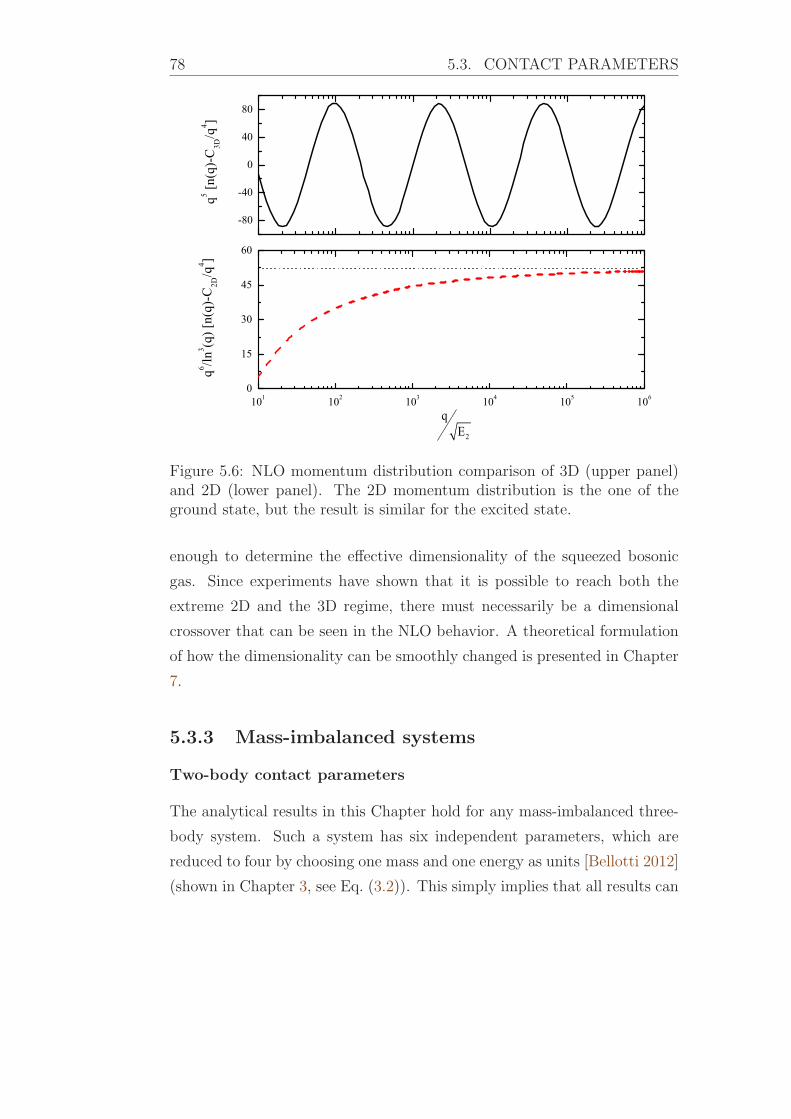
78 5.3. CONTACT PARAMETERS
101 102 103 104 105 1060
15
30
45
60
-80
-40
0
40
80
q5 [n(q
)-C
3D/q
4 ]q6 /ln
3 (q) [
n(q)
-C2D
/q4 ]
2
qE
Figure 5.6: NLO momentum distribution comparison of 3D (upper panel)and 2D (lower panel). The 2D momentum distribution is the one of theground state, but the result is similar for the excited state.
enough to determine the effective dimensionality of the squeezed bosonic
gas. Since experiments have shown that it is possible to reach both the
extreme 2D and the 3D regime, there must necessarily be a dimensional
crossover that can be seen in the NLO behavior. A theoretical formulation
of how the dimensionality can be smoothly changed is presented in Chapter
7.
5.3.3 Mass-imbalanced systems
Two-body contact parameters
The analytical results in this Chapter hold for any mass-imbalanced three-
body system. Such a system has six independent parameters, which are
reduced to four by choosing one mass and one energy as units [Bellotti 2012]
(shown in Chapter 3, see Eq. (3.2)). This simply implies that all results can

CHAPTER 5. MOMENTUM DISTRIBUTION IN 2D 79
be expressed as ratios of masses and energies, and in this way provides very
useful scaling relations. However, results depending on four independent
parameters are still hard to display and digest.
A systems composed of two identical particles, a, and a distinct one, c,
has from the beginning four independent parameters, which are reduced to
two after the choice of units. From now on, Eac and ma are the energy and
mass units, and to simplify the notation, the mass ratio m = mc
mais defined.
In this case, the two-body contact parameters in Eqs.(5.37) to (5.39) are
given by
Caa = 16π ( m
1 +m)2∫ ∞
0
dk k ∣fa(k)∣2 , (5.50)
Cac = Caa
2+ 2π∫
∞0
dk k ∣fc(k)∣2 , (5.51)
As shown in the previous section, for three identical particles where all
masses and interactions are the same, Caa = Cac = C2, and the quantityC2
E3is a universal constant in 2D [Bellotti 2013a], since it does not depend
on the quantum state considered. Maintaining universal conditions for all
excited states in mass-imbalanced systems, which have more excited states
[Bellotti 2012,Bellotti 2013b], must be more demanding.
Detailed investigations reveal that when the mass-energy symmetry is
broken, meaning that particles and two-body energies are not identical, the
universality of C2
E3does not hold anymore. The two two-body contact pa-
rameters defined in Eqs. (5.50) and (5.51) divided by the three-body energy
are not the same for all possible bound states in this general case. How-
ever, at least in one special case of two identical non-interacting particles,
Eaa = 0, the universality is recovered. This condition leads to fc = 0 in the
set of coupled homogeneous integrals equations (2.70) and two universal
two-body contact parameters are related by
Cac = Caa
2for Eaa = 0 . (5.52)
The effect of the two-body energy on the contact parameter is shown

80 5.3. CONTACT PARAMETERS
in Fig. 5.7 for the 133Cs133Cs6Li system, where a =133Cs and c =6Li. This
system has four excited states in both cases of Eaa = Eac and Eaa = 0
and the coefficients (two-body contact) of the large-momentum limit reach
constants in all cases. For Eaa = 0, universality is observed, since all two-
body contacts ratios, Cac/E3, are equal in units of the three-body energy.
This case is rather special because two particles do not interact and the
three-body structure is determined by the identical two-body interactions
in the identical subsystems. In other words the large-momentum limit of the
one-body density for particle a is determined universally by the properties
of the ac subsystem. The other contact parameter, Caa/E3, is also universal
and follows from Eq. (5.52).
This picture changes when Eaa = Eac, as seen in Fig. 5.7. Now, in the
large-momentum limit, the coefficients Caa and Cac of the one-body densities
change with the excitation energy. The systematics is that both Caa/E3 and
Cac/E3 as function of excitation energy move towards the corresponding
values for Eaa = 0, one from below and the other from above. First the
non-universality of the ratios with the two-body energies is understandable,
since the interaction of the two identical particles now must affect the three-
body structure at small distances, and hence at large momenta. However,
as the three-body binding energy decreases, the size of the system increases
and details of the short-distance structure becomes less important.
The quantities Caa
E3and 2π
E3∫ ∞0 dk k ∣fc(k)∣2 are defined by the limit of
large-q in n2 in Eq. (5.22). Plotting the corresponding pieces of n2(q)q4 as
function of q lead to figures similar to Fig. 5.7, where the different bound
state excitations show distinct results for Eaa = Eac, while they all coincide
for Eaa = 0. The ratio of the coefficients Cac
E3, Caa
E3and 2π
E3∫ ∞0 dk k ∣fc(k)∣2
are shown in table 5.1. The results are presented for two different two-body
energies and two different systems represented by c =6Li, a =133Cs or a =40K.
These numerical calculations confirm the systematics described above in
complete agreement with Eqs. (5.51) and (5.52).
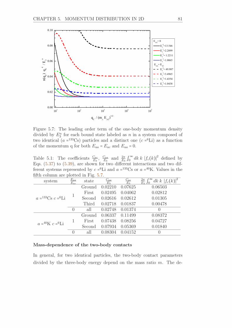
CHAPTER 5. MOMENTUM DISTRIBUTION IN 2D 81
101 102 103 104 1050.00
0.02
0.04
0.06
0.08
0.10
EAA
= 0
E30=13.546
E31=2.2899
E32= 1.2211
E33=1.0065
EAA
= EAC
E30= 49.987
E31=3.4965
E32=1.4354
E33=1.0438
n(q C
) q C
4 / E
3n
qC
/ (m EC)1/2
Figure 5.7: The leading order term of the one-body momentum densitydivided by En
3for each bound state labeled as n in a system composed of
two identical (a =133Cs) particles and a distinct one (c =6Li) as a functionof the momentum q for both Eaa = Eac and Eaa = 0.Table 5.1: The coefficients Cac
E3, Caa
E3and 2π
E3∫ ∞0 dk k ∣fc(k)∣2 defined by
Eqs. (5.37) to (5.39), are shown for two different interactions and two dif-ferent systems represented by c =6Li and a =133Cs or a =40K. Values in thefifth column are plotted in Fig. 5.7.
system Eaa
Eacstate Caa
E3
Cac
E3
2πE3∫ ∞0 dk k ∣fc(k)∣2
a =133Cs c =6Li 1
Ground 0.02210 0.07625 0.06503First 0.02495 0.04062 0.02812Second 0.02616 0.02612 0.01305Third 0.02718 0.01837 0.00478
0 all 0.02748 0.01374 0
a =40K c =6Li 1Ground 0.06337 0.11499 0.08372First 0.07438 0.08256 0.04727Second 0.07934 0.05369 0.01840
0 all 0.08304 0.04152 0
Mass-dependence of the two-body contacts
In general, for two identical particles, the two-body contact parameters
divided by the three-body energy depend on the mass ratio m. The de-

82 5.3. CONTACT PARAMETERS
pendence change from universal for Eaa = 0 to non-universal for Eaa = Eac.
The mass dependence for ground states are shown in Fig. 5.8, where the
ratio Caa
Cac= 2 in Eq. (5.52) is shown to hold for Eaa = 0 in the entire mass
interval investigated. It is also possible to see how the second term on the
right-hand-side of Eq. (5.51) affects the relation between the two two-body
contact parameters. Fig. 5.8 shows that the values rapidly increase from
small m up to 1 and become almost constant above m ≈ 5. This behavior
is similar to mass-imbalanced system in 3D [Yamashita 2013].
10-2 10-1 100 101 10210-3
10-2
10-1
100
EAA
= 0 C
AA
CAC
EAA
= EAC
CAA
CAC
C2 /
E 3
m
Figure 5.8: The two-body parameters Caa and Cac defined in Eqs. (5.50)and (5.51) as function of the mass ratio m = mc
mafor an aac system in both
cases where Eaa = 0 and Eaa = Eac.
Estimate of the two-body contact in the ground state
The parametrization of the ground state spectator function in Eq. (5.15) is
used to estimate the dependence of the two-body contact parameter on the

CHAPTER 5. MOMENTUM DISTRIBUTION IN 2D 83
three-body energy. Inserting it in Eq. (5.50) gives
Caa
E3
= 16π m2
(1 +m)(2 +m)f 2
a(0)(1 + 2
ln(E3) + 2
ln2(E3)) . (5.53)
A comparison between this approximation and the numerical results is
shown in Fig. 5.9. Notice that Eq. (5.53) provides a fairly good esti-
mate, which is accurate within 5% for small m, around 10% for m > 1, andwithin about 20% deviation in the worst case of m = 1. The divergence in
Eq. (5.53) for E3 → 1 means that the two-body contact parameters diverge
when the three-body system approaches the threshold of binding. This does
not reveal the full energy dependence since the normalization factor, f 2a(0),
also is state and energy dependent.
10-2 10-1 100 1010.0
0.1
0.2
0.3
0.4
0.5
numeric analytic
CA
A /
E 3
m
Figure 5.9: Comparison between the analytic estimative of Caa, given byEq. (5.53) and the numerical calculation from Eq. (5.50).

84 5.3. CONTACT PARAMETERS
Three-body contact parameters
The non-universality of the two-body contact parameters, and even of the
three-body one for identical particles (see Eq. (5.47)), does not encour-
age to check the universality of the three-body contact parameter in mass-
asymmetric systems. However, at least the system with two non-interacting
identical particles turned out to be universal and may lead to an interesting
large-momentum three-body structure. As before, inserting Eaa = 0 in the
set of coupled integral equations (2.70) gives fc(qc) = 0. Then Eqs. (5.16) to
(5.19) show directly that n1(qc) and n3(qc) vanish when fc(qc) = 0, leavingonly contributions from n4(qc) and n5(qc).
The sub-leading order of the large-momentum distribution multiplied
by q6c / ln3(qc) is shown in Fig. 5.10 , that is Caa,c, as functions of qc for the
four bound states of the system a =133Cs and c =6Li for both Eaa = Eac
and Eaa = 0. Only one of these three-body contact parameters is shown,
since the other one, Cac,a, is related state-by-state through the mass factors
in Eqs. (5.42) and (5.43). The momentum dependence flattens at much
larger qc is not shown in figure. The values are divided by the three-body
energy and no simple energy scaling were obtained. Not surprisingly, a more
complicated and non-universal behavior is present.
However, it is striking to see that this sub-leading order in the large-
momentum limit is negligibly small for Eaa = 0 compared to the interacting
case with Eaa = Eac. This suggests that a negligible three-body contact
parameter combined with a universal two-body contact parameter can be
taken as a signature of a two-body non-interacting subsystem within a three-
body system in 2D.

CHAPTER 5. MOMENTUM DISTRIBUTION IN 2D 85
101 102 103 104 10510-5
10-4
10-3
10-2
10-1
100
EAA
= 0
E3
0=13.546
E3
1=2.2899
E3
2= 1.2211
E3
3=1.0065 E
AA= E
AC
E3
0= 49.987
E3
1=3.4965
E3
2=1.4354
E3
3=1.0438
[n(q
C) -
CA
A /
q C4 ] q
C6 /
ln3 (q
C) /
E3n
qC
/ (m EC)1/2
Figure 5.10: The sub-leading order of the one-body momentum densitydivided by En
3for each bound state labeled as n in a system composed of
two identical particles (a =133Cs) and a distinct one (c =6Li) as a functionof the momentum q for both Eaa = Eac and Eaa = 0.5.4 Discussion about possible experiments
As demonstrated in Sec. 5.3.3, the NLO term in the momentum distribution
can be used to distinguish whether the two-body subsystems are interacting
when three-body systems are being taken into account. Maybe more impor-
tant, the NLO term also carries a tell-tale signature of the dimensionality
of the quantum system under study. The 2D to 3D crossover was studied
in Ref. [Dyke 2011, Sommer 2012], and it has been shown that both the
3D and the strict 2D limits are accessible in experiments. The crossover
was here discussed by using formalism applicable to either pure 2D or pure
3D without explicit consideration of the external confinement. The results
predict that a proof-of-principle experiment is possible by going to the two
strict limits. However, the full crossover including the intermediate regime
(quasi-2D) where the transverse confinement must be taken explicitly into
account, which is experimentally addressable, should be explored theoreti-

86 5.4. DISCUSSION ABOUT POSSIBLE EXPERIMENTS
cally in the future. A first step in this direction is taken in [Yamashita 2014]
and discussed in Chapter 7.
The units (the dimer binding energy E2) and the effects of the transverse
confinement on this two-body bound state need to be considered when con-
necting the results to the experiments. The interaction is controlled by Fes-
hbach resonances [Chin 2010]. However, under the confinement, the dimer
energy is modified and becomes E2 = Bhωz exp(−√2πlz/∣a∣)/π [Petrov 2001].
Here, ωz is the transverse harmonic confinement frequency, lz =√h/mωz the
trapping length, a the 3D scattering length associated with the Feshbach res-
onance and B = 0.905 is a constant. This formula holds for a < 0 and ∣a∣≪ lz,
while on resonance, ∣a∣→∞ and E2 = 0.244hωz. Corrections also arise from
the non-harmonic optical lattice, but they are not essential for the discussion
which follows. The dimer energy scale can be converted into a momentum
scale, k0, through E2 = h2k20/2m. Accessing the tail behavior and the 2D-3D
crossover, the range k ∼ 101−103k0 is enough, as shown in Figs. 5.5 and 5.6.
Some 2D Bose gas experiments [Hung 2011, Yefsah 2011] use lz ∼ 3800a0,
where a0 is the Bohr radius, which implies that k0 ∼ 10−4a−10 when ∣a∣ =∞.
For the momentum distribution measurements [Stewart 2010,Kuhnle 2010],
the maximum momentum reported is about k ∼ 10−3a−10. This implies that
an order of magnitude or two beyond the reported capabilities is necessary.
However, if a is tuned away from resonance to the a < 0 side, E2 will de-
crease rapidly according to the formulas above, inducing a corresponding
rapid decrease of k0 which should render the physics discussed here within
reach of current experimental setups. Notice that the van der Waals length
scale of about 100a0 is in the deep tail, so there is no conflict with the
universal zero-range description employed here.

Chapter 6
Momentum distribution in 3D
A key result in the study of the two-dimensional (2D) one-body density is
the analytic expression of the large-momentum asymptotic behavior for the
spectator functions. In Chapter 5, mass-imbalanced systems were addressed
and it was shown that the spectator functions have the same asymptotic
behavior, i.e., ln(q)/q2, each one having specific normalization constants,
irrespective of the quantum state considered, with a relation among them.
Three-dimensional (3D) three-body systems have geometric scaling be-
tween consecutive three-body states for ∣a∣→∞, as predicted in the seventies
by V. Efimov [Efimov 1970] and firstly observed in cold atomic gases around
35 years latter [Kraemer 2006]. The experimental verification of the effect
has opened a new research direction dubbed Efimov physics [Ferlaino 2010].
In practice, the Efimov effect occurs when the size of the three-body system,
given for the scattering length ∣a∣ is much larger than interaction range r0,
i.e., ∣a∣/r0 →∞. In this limit, a sequence of three-body bound states occurs
wherein two successive states always have the same fixed ratio of their bind-
ing energies. The scaling of the energy levels implies that some of properties
of three-body 3D systems are universal, in the sense that are independent
of the state considered once properly rescaled. The focus here is in the two-
and three- body contact parameters, defined via the one-body momentum
density.
The two- and three-body contact parameters were determined for a 3D
system of three identical bosons in Ref. [Castin 2011] and for mixed-species
systems in Ref. [Yamashita 2013]. Unlike the 2D analogue, the results show
that the influence of non-equal masses in three-body systems goes beyond
changing the contact parameters values, i.e., the sub-leading term in the
87

88 6.1. FORMALISM AND DEFINITIONS
one-body momentum distribution, which defines C3, has a different and
mass-dependent functional form in each case.
The study is taken for three-body bound Efimov-like states for systems
that contain two identical bosons and a third distinguishable particle. The
contact parameters of such systems are addressed when the masses are dif-
ferent and for different strengths of the interaction parameters. For that
aim the one-body momentum distributions are computed and its asymp-
totic behavior is studied. Only the universal regime is considered, since all
two-body potentials are described by zero-range interactions. Results are
shown for the experimentally relevant cases 6Li133Cs133Cs and 6Li87Rb87Rb,
as in Chapter 5.
6.1 Formalism and definitions
The AAB system is constituted by two identical bosons A and a third par-
ticle B of different kind. The universal limit ∣a∣≫ r0, where the range of the
two-body potentials can be neglected, is naturally achieved by introducing
zero-range interactions between the particles.
The set of 3D homogeneous integral equations are given by Eq. (2.83) for
a general system of three distinguishable particles. For the AAB system, the
s−wave coupled subtracted integral equations for the spectator functions,
χ, corresponding to a bound state, where ∣E3∣ is the absolute value of the
three-body energy, is written in units of h =mA = 1 as
χAA(y) = 2τAA(y; ∣E3∣)∫ ∞0
dxx
yG1(y, x; ∣E3∣)χAB(x) , (6.1)
χAB(y) = τAB(y; ∣E3∣)∫ ∞0
dxx
y[G1(x, y; ∣E3∣)χAA(x)+ AG2(y, x; ∣E3∣)χAB(x)] , (6.2)

CHAPTER 6. MOMENTUM DISTRIBUTION IN 3D 89
with
τAA(y; ∣E3∣) ≡ 1
π
⎡⎢⎢⎢⎢⎣√∣E3∣ + A + 2
4A y2 ∓√EAA
⎤⎥⎥⎥⎥⎦−1, (6.3)
τAB(y; ∣E3∣) ≡ 1
π(A + 1
2A )3/2 [√∣E3∣ + A + 2
2(A + 1)y2 ∓√EAB]
−1, (6.4)
G1(y, x; ∣E3∣) ≡ ln2A(∣E3∣ + x2 + xy) + y2(A + 1)2A(∣E3∣ + x2 − xy) + y2(A + 1)− ln
2A(µ2 + x2 + xy) + y2(A + 1)2A(µ2 + x2 − xy) + y2(A + 1) , (6.5)
G2(y, x; ∣E3∣) ≡ ln2(A∣E3∣ + xy) + (y2 + x2)(A + 1)2(A∣E3∣ − xy) + (y2 + x2)(A + 1)− ln
2(Aµ2 + xy) + (y2 + x2)(A + 1)2(Aµ2 − xy) + (y2 + x2)(A + 1) , (6.6)
where x and y denote dimensionless momenta and A is the mass ratio
A = mB/mA. Notice that a slightly different notation is introduced for the
study of the 3D system, in order to avoid confusion with the previous 2D
case.
The interaction strengths of theAA andAB subsystems are parametrized
by the energies EAA and EAB, and the plus and minus signs in Eqs. (6.3)
and (6.4) refer to virtual and bound two-body subsystems, respectively [Ya-
mashita 2002,Bringas 2004,Yamashita 2008].
The universal regime of the AB system is studied with ∣aAB ∣→∞ and/or
EAB → 0. In light of the fact that experimental information about mixed
systems of the AAB type is still sparse, the two extreme cases of i) EAA = 0and ii) a non-interacting AA subsystem are considered. Notice that condi-
tions i) and ii) are equivalent in 2D systems [Bellotti 2014], while they are
distinct in 3D.
As before, qα is the Jacobi momentum from α particle to the center-of-
mass of the pair (βγ) and pα the relative momentum of the pair. The four
terms in the one-body momentum density for each constituent are defined

90 6.2. ASYMPTOTIC SPECTATOR FUNCTION
in the most general case of three distinguishable particles in Eqs. (5.16) to
(5.19). The AAB system has only two distinct distributions, namely of type
α = β = A and type γ = B. Following the notation and units defined in this
Chapter, the wave function in Eq. (2.67) is written in terms of the spectator
functions in the basis ∣qBpB⟩ as⟨qBpB ∣Ψ⟩ = χAA(qB) + χAB(qA) + χAB(q′A)∣E3∣ +H0
,
= χAA(qB) + χAB(∣pB −qB
2∣) + χAB(∣pB +
qB
2∣)∣E3∣ +H0
, (6.7)
or in the basis ∣qApA⟩ as⟨qApA∣Ψ⟩ = χAA(∣pA −
AA+1qA∣) + χAB(∣pA +1A+1qA∣) + χAB(qA)∣E3∣ +H ′0 , (6.8)
where H0 = p2B2mAA
+q2B
2mAA,Band H ′
0= p2A
2mAB+
q2A2mAB,A
. The reduced masses are
given by mAA = 1
2, mAA,B = 2AA+2 , mAB = AA+1 and mAB,A = A+1A+2 .
The momentum distributions for the particles A and B are
n(qB) = ∫ d3pB ∣⟨qBpB ∣Ψ⟩∣2, n(qA) = ∫ d3pA∣⟨qApA∣Ψ⟩∣2 (6.9)
and they are normalized such that ∫ d3q n(q) = 1.Since the results here are compared to Ref. [Castin 2011], note that the
definition of momentum distributions as well as their normalizations differ
for factor of 1/(2π)3 multiplying the definition of n(q), which is normalized
to 3, the number of particles, in that reference.
6.2 Asymptotic spectator function
The asymptotic behavior of the spectator function is used in deriving some
analytic formulas and compare to corresponding numerical results. The
large momentum regime√∣E3∣ ≪ q is accessed by taking the limit µ →
∞ and ∣E3∣ = EAA = EAB → 0. The coupled equations for the spectator

CHAPTER 6. MOMENTUM DISTRIBUTION IN 3D 91
functions in Eqs. (6.1) and (6.2) consequently simplify and become
χAA(y) = 2
π
⎡⎢⎢⎢⎢⎣y√A + 2
4A⎤⎥⎥⎥⎥⎦−1∫∞
0
dxx
yG1a(y, x)χAB(x) , (6.10)
χAB(y) = 1
π(A + 1
2A )3/2 [y√ A + 2
2(A + 1)]−1×
∫∞
0
dxx
y[G1a(x, y)χAA(x) +AG2a(y, x)χAB(x)] , (6.11)
where
G1a(y, x) ≡ ln 2A(x2 + xy) + y2(A + 1)2A(x2 − xy) + y2(A + 1) , (6.12)
G2a(y, x) ≡ ln (y2 + x2)(A + 1) + 2xy(y2 + x2)(A + 1) − 2xy . (6.13)
The coupled equations in Eqs. (6.10) and (6.11) are solved by using the
ansatz
χAA(y) = cAA y−2+ıs and χAB(y) = cAB y
−2+ıs, (6.14)
where y once again denotes a dimensionless momentum. Inserting the func-
tions (6.14) in the set of coupled equations and performing the scale trans-
formation x = y z in the integrand of Eqs. (6.10) and (6.11), it is derived
the set of equations for the constants cAA and cAB, given by
cAA =cAB
2
π
√4AA + 2 ∫
∞0
dz z−2+1+ıs ln2A(z2 + z) + (A + 1)2A(z2 − z) + (A + 1) , (6.15)
cAB = 1π(A + 1
2A )3/2√2(A + 1)A + 2 ∫
∞0
dz z−2+1+ıs [cAA ln2A(1 + z) + z2(A + 1)2A(1 − z) + z2(A + 1)
+ A cAB ln(1 + z2)(A + 1) + 2z(1 + z2)(A + 1) − 2z ] . (6.16)
Returning to Eqs. (6.10) and (6.11), there are two solutions which are
complex conjugates of each other, i.e., z±ıs. Apart from an overall nor-
malization, there is still a relative phase between these two independent
solutions, which is determined by requiring the wave function to be zero at

92 6.2. ASYMPTOTIC SPECTATOR FUNCTION
a certain momentum denoted q∗. This parameter is known as the three-
body parameter [Nielsen 2001,Braaten 2006]. This is the momentum-space
equivalent of the coordinate-space three-body parameter which is now be-
lieved to be simply related to the van der Waals two-body interaction of the
atoms in question [Berninger 2011a,Schmidt 2012b,Sørensen 2013]. In this
case the asymptotic form of the spectator functions becomes
χAA(q) = cAA q−2 sin(s ln q/q∗) and χAB(q) = cAB q
−2 sin(s ln q/q∗) ,(6.17)
where q denotes momentum and the boundary condition χ(q∗) = 0 is ful-
filled.
10-2 10-1 100 101 102 103 104 105 106
-1
0
1
2
Rb-Rb-LiSixth excited state
q2 BAA
qB /
(a) Sixth excited state, E3 = −8.6724 ×10⁻¹² for a Rb-Rb-Li molecule.
10-1 100 101 102 103 104 105 106
-1
0
1
2
3
Cs-Cs-LiEighth excited state
q2 BAA
qB /
(b) Eighth excited state, E3 = −8.9265 ×10⁻¹³ for a Cs-Cs-Li molecule.
Figure 6.1: The spectator function χAA(q) of a high excited state for EAA =EAB = 0, solution of the coupled equations (6.1) and (6.2) (solid line),compared with the asymptotic formula (6.14) (dotted line). E3 energies aregiven in arbitrary units.
The asymptotic form of the spectator function should be compared with
the solutions of the subtracted equations in the limit of large momentum,
constrained by the window κ0 << qB << µ, where κ0 ≡√∣E3∣. The spectator
functions χAA(q) for Rb-Rb-Li and Cs-Cs-Li compared to the respective
asymptotic formula are shown in Fig. 6.1. The difference between the nu-
merical calculation and the analytic behavior is easily understood. While

CHAPTER 6. MOMENTUM DISTRIBUTION IN 3D 93
the limit µ→∞ in taken in the analytical derivations, µ2 = 1 is used for the
subtraction point in the numerical calculation (see for instance Ref. [Fred-
erico 2012] for a detailed discussion and references therein). Notice that
this subtraction method is basically equivalent to the procedure employed
by Danilov [Danilov 1961] to regularize the original three-body Skorniakov-
Ter-Martirosian equation [Skornyakov 1956]. A very detailed discussion of
these issues is given by Pricoupenko [Pricoupenko 2010,Pricoupenko 2011].
Therefore, the two curves would coincide in the idealized limit where κ0 = 0and µ → ∞ and the effect of finite value of these two quantities is seen on
each end of both plots. The window of validity for the use of the asymptotic
formulas, i.e.,√∣E3∣ << q << µ can be clearly seen in these figures.
6.2.1 Scaling parameter
Although the asymptotic expression in Eq. (6.17) is already known, the
procedure of using it to solve the coupled integral equations in Eqs. (6.10)
and (6.11) leads to an expression for the scaling parameter s of an AAB
system. Inserting Eq. (6.15) into Eq. (6.16), the set of coupled equations
can be written as a single transcendental equation
1
π(A + 1
2A )3/2√2(A + 1)A + 2 ⎛⎝AI1(s) + 2
π
√4AA + 2I2(s)I3(s)⎞⎠ = 1 , (6.18)
where
I1(s) = ∫ ∞0
dzz−1+is ln [(z2 + 1)(A + 1) + 2z(z2 + 1)(A + 1) − 2z ] = 2π
s
sinh(θ1s − π2s)
cosh(π2s) , (6.19)
I2(s) = ∫ ∞0
dzz−1+is ln [2A(z2 + z) +A + 12A(z2 − z) +A + 1]
= 2π
s
sinh(θ2s − π2s)
cosh(π2s) (A + 1
2A )is/2
, (6.20)

94 6.2. ASYMPTOTIC SPECTATOR FUNCTION
I3(s) = ∫ ∞0
dzz−1+is ln [2A(1 + z) + (A + 1)z22A(1 − z) + (A + 1)z2 ]
= 2π
s
sinh(θ2s − π2s)
cosh(π2s) (A + 1
2A )−is/2
. (6.21)
The angles are given by tan2 θ1 = A(A+2) and tan2 θ2 = (A+2)/A with the
conditions π/2 < θ1 and θ2 < π. For the special case of equal masses, i.e.,
A = 1, θ1 = θ2, I1 = I2 = I3 and
⎛⎝ 1π√
4
3I1(s)⎞⎠ + 2⎛⎝ 1π
√4
3I1(s)⎞⎠
2
− 1 = 0, (6.22)
for which the physically relevant solution is seen to be
1
π
√4
3I1(s) = 1
2. (6.23)
The Efimov equation for the scaling parameter s in a system of iden-
tical bosons is then recovered from Eqs. (6.19) and (6.23) [Efimov 1970,
Nielsen 2001]. Another very interesting and relevant case is when there
is no interaction between the two A particles, in which case cAA = 0 in
Eq. (6.16). The equation for the scale factor, Eq. (6.18), now simplifies and
gives Aπ(A + 1
2A )3/2√2(A + 1)A + 2 I1(s) = 1. (6.24)
The scaling factors, exp(π/s), are plotted in Fig. 6.2 for the cases when
all three subsystems have resonant interaction, which is the expression in
Eq. (6.18) valid for EAA = EAB = 0 (solid line) and when there is no inter-
action in the AA subsystem, which is the expression in Eq. (6.24) valid for
EAB = 0 (dashed line).
What is important to notice is that for mA ≫ mB (A ≪ 1), the scaling
factors are very similar, and both are much smaller than the equal mass case
where A = 1. Therefore, it is expected that the AAB system with heavy A
and light B, would have many universal three-body bound states (s large or

CHAPTER 6. MOMENTUM DISTRIBUTION IN 3D 95
0.01 0.1 1 10 1000
5
10
15
20
25
Rb-Rb-Li
Cs-Cs-Li EAA = 0 No AA interaction
exp(
/s)
A
Figure 6.2: Scaling parameter s as a function of A = mB/mA for EAA = 0and EAB = 0(resonant interactions), solid line, and for the situation whereEAB = 0 but with no interaction between AA, dashed line. The arrows showthe corresponding mass ratios for 133Cs-133Cs-6Li and 87Rb-87Rb-6Li.
equivalently eπ/s small) irrespective of whether the heavy-heavy subsystem
is weakly or strongly interacting. This feature is similar to the 2D case and
recent experiments with mixtures of 6Li and 133Cs indicate that there could
be a resonance of the 6Li-133Cs subsystem at a point where the scattering
length in the 133Cs-133Cs system is close to zero, i.e., weak interaction in
the AA subsystem [Repp 2013,Tung 2013].
6.3 Asymptotic one-body densities
The large-momentum one-body density n(qB), i.e., the single-particle mo-
mentum distribution for particle B is calculated similarly to the procedure
used for the 2D case. From Eqs. (6.7) and (6.9) it is possible to split the

96 6.3. ASYMPTOTIC ONE-BODY DENSITIES
momentum density into nine terms, which can be reduced to four consid-
ering the symmetry between the two identical particles A. This simplifies
the computation of the momentum density to the form n(qB) = ∑4
i=1 ni(qB),where
n1(qB) = ∣χAA(qB)∣2∫ d3pB1
(∣E3∣ + p2B + q2B A+24A )2 = π2∣χAA(qB)∣2√∣E3∣ + q2B A+24A
,
(6.25)
n2(qB) = 2∫ d3pB∣χAB(∣pB −
qB
2∣)∣2
(∣E3∣ + p2B + q2B A+24A )2 , (6.26)
n3(qB) = 2 χ∗AA(qB)∫ d3pBχAB(∣pB −
qB
2∣)
(∣E3∣ + p2B + q2B A+24A )2 + c.c. , (6.27)
n4(qB) = ∫ d3pBχ∗AB(∣pB −
qB
2∣)χAB(∣pB +
qB
2∣)
(∣E3∣ + p2B + q2B A+24A )2 + c.c. . (6.28)
Going to the large momentum domain, q ≫ √∣E3∣, the limit ∣E3∣ → 0
is taken, i.e., the three-body energy is assumed to be negligible, since the
focus is the imprint of excited Efimov states on the momentum distribu-
tion. These states are very extended and do not feel any short-range effects
besides those encoded in the three-body parameter, q∗, discussed above.
The asymptotic forms for the spectator functions are used in the inte-
grals of Eqs. (6.25) to (6.28), where the integration is being performed from
0 to ∞. This may a priori cause problems at small momenta. However, a
numerical check shows that the different behavior of the spectator functions
at low momenta contributes only at next-to-next-to-leading order (NNLO).
This procedure is the same as the one used in Ref. [Castin 2011].
The large momentum limit of the four terms in Eqs. (6.25) to (6.28)
is worked out in Appendix E, which is supplemented by Appendix F. The
derivation of the large momentum contributions of the terms n3(qB) (seeEq. (6.27)) and n4(qB) (see Eq. (6.28)) require several non-trivial mathe-
matical steps, which let them too long and make the presentation lengthly
in the bulk of the Chapter. However, it is worth to emphasize that the equa-

CHAPTER 6. MOMENTUM DISTRIBUTION IN 3D 97
tions derived in Appendix E are the basis of the following discussion and
their tricky derivation deserves to be looked out. Then, the large momentum
contribution of the four terms in Eqs. (6.25) to (6.28) up to next-to-leading
order (NLO) is found to be
⟨n1(qB)⟩ = π2
q5B∣cAA∣2
√ AA + 2 , (6.29)
⟨n2(qB)⟩ = 8A2
q4B (A + 1)2 ∫ d3qA ∣χAB(qA)∣2−8π2 ∣cAB ∣2
q5B
A3(A + 3)(A + 1)3√A(A + 2) , (6.30)
⟨n3(qB)⟩ = 4π2cAA cAB
q5B cosh ( sπ2)⎧⎪⎪⎨⎪⎪⎩√ AA + 2 cos⎛⎝s ln
√A + 12A ⎞⎠ cosh [s(π2 − θ3)]
+ sin⎛⎝s ln
√A + 12A ⎞⎠ sinh [s(π2 − θ3)]
⎫⎪⎪⎬⎪⎪⎭ , (6.31)
⟨n4(qB)⟩ = 8π2∣cAB ∣2A2
s q5B
√A(A + 2) cosh ( sπ2) {√A(A + 2) sinh [s(π
2− θ4)]
−s AA + 1 cosh [s(π2 − θ4)]} , (6.32)
where tan θ3 = √A+2A for 0 ≤ θ3 ≤ π/2 and tan θ4 = √A(A + 2) for 0 ≤ θ4 ≤π/2.
6.4 Leading and sub-leading terms
As discussed in Sec. 5.3.2, the leading order term Cq4B
has the same func-
tional form as in 2D and comes only from n2, i.e., the first term on the
right-hand-side of Eq. (6.30). The constant C is simply given by C =8A2
(A+1)2 ∫ d3qA ∣χAB(qA)∣2, which gives C/κ0 = 0.0274 for 133Cs-133Cs-6Li and
C/κ0 = 0.0211 for 87Rb-87Rb-6Li. For A = 1, the value 3(2π)3C/κ0 = 52.8 is
close to the exact value 53.097, obtained in Ref. [Castin 2011]. The factor
3(2π)3 comes from the different choice of normalization.
The small discrepancy from both values of the contact parameter for a

98 6.4. LEADING AND SUB-LEADING TERMS
system composed for identical bosons arises from numerical issues. While
the numerical value obtained here is calculated for the second excited state,
the exact value in Ref. [Castin 2011] is calculated for an arbitrary highly
excited state.
In Fig. 6.3 is shown the value of C/κ0 for mass ratios in the range
6/133 ≤ A ≤ 25. The increase is very rapid until A ≈ 5, beyond which an
almost constant value is reached. A similar behavior is found in 2D, as
shown in Fig. 5.8.
0 5 10 15 20 250.02
0.03
0.04
0.05
0.06
0.07
0.08
0.09
C/
0
A
Figure 6.3: C/κ0 for mass ratios in the range 6/133 ≤ A ≤ 25.In Ref. [Castin 2011] it is shown that the non-oscillatory term of order
q−5B coming from n1 to n4 exactly cancels for A = 1. However, this conclusiondoes not hold in the general case A ≠ 1, as demonstrated bellow.
The four analytic expressions derived for each of the components of the
one-body momentum distribution in Sec. 6.3 are defined apart the coeffi-
cients caa and cab. The ratio between these coefficients is given by Eq. (6.15),

CHAPTER 6. MOMENTUM DISTRIBUTION IN 3D 99
which can be used to eliminate one of these factors. The other one can be
determined from the overall normalization of the wave function. As the
study is focused on the general behavior of the momentum distribution, the
normalization is not relevant and the remaining coefficient is set to unit
from now on, i.e., cAB = 1.The contribution −(n1+n2+n3) and n4 are shown in Fig. 6.4 as a function
of mass ratio A (each individual component ni as function of the mass ratio
A is shown in Fig. 6.5). What is immediately seen is that for A = 1 the
result of Ref. [Castin 2011] is reproduced, i.e., that the q−5B non-oscillatory
term cancels. However, for general A this does not hold and a q−5B term in
the asymptotic momentum distribution should also be expected for systems
with two identical and a third particle.
0.01 0.1 1 10 100
5
10
15
20
25
30
0.0 0.2 0.4 0.6 0.8 1.0 1.2 1.4 1.6 1.8 2.0-0.15
-0.10
-0.05
0.00
0.05
0.10
0.15
0.20
0.25
0.30
0.35
q5 B<n i>
A
-(<n1>+<n2>+<n3>)
<n4>
Figure 6.4: Non-oscillatory contributions for n1, n2, n3 and n4 as a functionof the mass ratio A. Their sum, showed in the inset, cancels exactly for A =0.2, 1 and 1.57.
This demonstrates that non-equal masses will generally influence not

100 6.4. LEADING AND SUB-LEADING TERMS
only the value of the contact parameter attributed to three-body bound
states but also the functional form of the asymptotic momentum tail. An-
other important difference between 2D and 3D system arises here. Remem-
ber that systems of non-equal masses have the same functional form of the
next-order contribution to the momentum distribution (see Sec. 5.2). Cu-
riously, there is an oscillatory behavior around A ∼ 1 from the sum of all
contributions. This is shown in the inset of Fig. 6.4 where zero-crossings
are seen at A = 0.2, 1, and 1.57. It seems quite clear that all the oscillatory
terms, which depend on the scale factor s, are the reason for this interesting
behavior, but a physical explanation for it was not found yet.
0.1 1 10 100-80
-60
-40
-20
0
20
40
<n2>
<n3>
<n1>
<n4>
q5 B<n i>
A
Figure 6.5: Individual non-oscillatory contributions for n1, n2, n3 and n4 asa function of the mass ratio A.
However, what makes this interesting is the fact that if ratios of typical
isotopes of alkali atoms like Li, Na, K, Rb, and Cs are taken, then one can
get rather close to 0.2 or 1.57. For instance, taking one 133Cs and two 85Rb
yields A = 1.565, while one 7Li atom and two 39K atoms yields A = 0.179.These interesting ratios are thus close to experimentally accessible species.

CHAPTER 6. MOMENTUM DISTRIBUTION IN 3D 101
6.5 Numerical examples
Some numerical examples of momentum distributions for the experimen-
tally interesting systems with large mass ratios are now provided. Focus
is on 133Cs-133Cs-6Li and 87Rb-87Rb-6Li systems, where two extreme pos-
sibilities are investigated: (i) the heavy-heavy subsystems, i.e., 133Cs-133Cs
and 87Rb-87Rb, have a two-body bound state at zero energy and (ii) the
opposite limit where they do not interact. In the first case the heavy atoms
are at a Feshbach resonance with infinite scattering length, while in the
second case they are far from resonance and a negligible background scat-
tering length is assumed. As it was recently demonstrated for the 133Cs-6Li
mixture, there are Feshbach resonances in the Li-Cs subsystem at positions
where the Cs-Cs scattering length is non-resonant [Repp 2013,Tung 2013].
While this does not automatically imply that the Cs-Cs channel can be ne-
glected, the assumption (ii) is made here. The formalism can be modified
in a straightforward manner to also include interaction in the heavy-heavy
subsystem.
As before the focus is on the AAB system, where A refers to the identical
(bosonic) atoms, 133Cs or 87Rb, and B to 6Li. By solving Eq. (6.18), the
scaling factors are s(6/133) = 2.00588 and s(6/87) = 1.68334 when assuming
that all three subsystems have large scattering lengths (solid line in Fig. 6.2).
The situation where the interaction between the two identical particles is
turned off is shown by the dashed line in Fig. 6.2. In this case, s(A) iscalculated from Eq. (6.16) by setting cAA = 0. This yields s(6/133) = 1.98572and s(6/87) = 1.63454.
Firstly the binding energies are considered. Assuming that the Cs-Cs
and Rb-Rb two-body energies are zero, a system satisfying the universality
condition ∣a∣ ≫ r0 implies that any observable should be a function of the
remaining two- and three-body scales, which can be conveniently chosen as
∣E3∣(N) and EAB (the Cs-Li or Rb-Li two-body energy). Here N denotes the
Nth consecutive three-body bound state with N = 0 being the lowest one.
Thus, the energy of an N +1 state can be plotted in terms of a scaling func-

102 6.5. NUMERICAL EXAMPLES
-0.2 0.0 0.2 0.4 0.6 0.8 1.00.0
0.1
0.2
0.3 Rb-Rb-Li Cs-Cs-Li
[(E(N
+1)
3-AB)/E
(N)
3]1/
2
[EAB/E(N)3
]1/2
1
2
3
4
5
6
Figure 6.6: EAB is the Cs-Li or Rb-Li two-body energy (Cs-Cs and Rb-Rb two-body energies are zero). The negative and positive parts refer,respectively, to virtual and bound AB states, such that ǫAB = 0 and ǫAB ≡EAB, respectively, on the negative and positive sides. The circles labeledfrom 1 to 6 mark the points where the momentum distributions have beencalculated.
tion relating only EAB and the energy of previous state. The limit cycle,
which should be in principle reached for N →∞, is achieved pretty fast such
that the curve in Fig. 6.6 is constructed using N = 2 [Yamashita 2002,Fred-
erico 2012]. In this figure, the negative and positive parts of the horizontal
axis refer, respectively, to virtual and bound two-body AB states. The cir-
cles labeled from 1 to 6 mark the points where the momentum distributions
have been calculated. The points 1 and 4 represent the Borromean case,
the points 2 and 5 are the “Efimov situation” and in points 3 and 6 AB is
bound.
Fig. 6.7(a) and 6.7(b) give the momentum distributions of the second ex-
cited states for the energy ratio√EAB/∣E3∣ given by the points labeled from

CHAPTER 6. MOMENTUM DISTRIBUTION IN 3D 103
0 20 40 60 80 100 120 140 160 180 20010-12
10-11
10-10
10-9
10-8
10-7
10-6
10-5
10-4
10-3
10-2
10-1
100
qA
qB
Cs-Cs-Li 1 2 3
n(q)
/n(0
)
q/0
(a) A =133Cs.
0 20 40 60 80 100 120 140 160 180 20010-12
10-11
10-10
10-9
10-8
10-7
10-6
10-5
10-4
10-3
10-2
10-1
100
qB
n(q)
/n(0
)
q/0
Rb-Rb-Li 4 5 6
qA
(b) A =87Rb.
Figure 6.7: Momentum distribution for the second excited state as a func-tion of the relative momentum of one A-particle, qA, or 6Li, qB, to thecenter-of-mass of the remaining pair A-6Li or A-A. The solid, dashed anddotted lines were calculated for the two- and three-body energies satisfyingthe ratios indicated by the points 1 to 3 (A =133Cs) and 4 to 6 (A =87Rb) inFig. 6.6. The circles show the set of curves related to qA or qB.
1 to 6 in Fig. 6.6. According to previous calculations [Yamashita 2004a],
for fixed three-body energy the size of the system increases as the num-
ber of bound two-body subsystems increase. Thus, it seems reasonable
that the Borromean case decreases slower. This behavior is clearly seen in
Figs. 6.7(a) and 6.7(b). The distance of one atom to the center-of-mass
of the other two is much larger for 6Li than for 133Cs or 87Rb, due to the
large difference of the masses. Therefore, the momentum distribution for
the heavier atom, qA set, decreases much slower than that for the lighter
one, qB set.
Figs. 6.8(a) and 6.8(b) show the rescaled momentum distributions for
the ground, first and second excited states. In these figures, the subsystem
energies are chosen to zero, corresponding to the transition point to a Bor-
romean configuration. In this situation, the only low-energy scale is ∣E3∣(remember that the high-momentum scale is µ = 1). Therefore, in units in
which ∣E3∣ = 1, to achieve a universal regime, in principle, to wash-out the
effect of the subtraction scale, µ, it is necessary to go to a highly excited
state. However, a universal low-energy regime of n(qB)/n(qB = 0) is seen

104 6.5. NUMERICAL EXAMPLES
0.0 0.5 1.0 1.5 2.0 2.5 3.00.0
0.2
0.4
0.6
0.8
1.0
qA
Cs-Cs-Li Ground First Second
n(q)
/n(0
)
q / 0
qB
(a) A =133Cs.
0 1 2 3 4 50.0
0.2
0.4
0.6
0.8
1.0
Rb-Rb-Li Ground First Second
n(q)
/n(0
)
q / 0
qB
qA
(b) A =87Rb.
Figure 6.8: Rescaled momentum distribution for the ground, first andsecond excited states as a function of the relative momenta of the A-particleto the center-of-mass of the pair 6Li-A, qA, and of 6Li to the center-of-massof the pair A-A, qB. The subsystem binding energies are all set to zero.Normalization to unity at zero momentum.
for momentum of the order of√∣E3∣, even for the ground state which is
smaller than excited states. Then, in practice, the universal behavior of the
momentum distribution is approached rapidly.
Chapter 7
Dimensional crossover
Examples of how the dimensionality affects the properties of physical sys-
tem have been recently attracting great interest, since the possibility of
probing lower dimensional systems has being continuously increasing. One
recent and famous example is graphene, which is itself a effective two-
dimensional (2D) structure with good mechanical and electrical proper-
ties [Novoselov 2004]. Besides that, the experimental study of one-dimensional
(1D) systems, which is an useful theoretical laboratory to study physical
problems, has also been recently reported [Serwane 2011, Zurn 2012]. Fol-
lowing this line, maybe the most surprisingly achievement is the study of
the so-called quantum dots [Ramos 2011], which are approached as zero-
dimensional systems.
Dimensionality also plays an important role in the behavior of few- and
many-body quantum systems. As it was discussed in Chapters 3 and 6,
the Efimov effect [Efimov 1970], where a geometric series of three-body
bound states of three bosons occurs at the threshold for binding the two-
body subsystems, is present in 3D systems but absent when the dimension is
reduced to two. A straightforward consequence discussed in Chapters 5 and
6 is that systems restricted to different dimensions have very distinct two-
and three-body contact parameters and asymptotic forms of the momentum
distribution at the next-to-leading order. The contact parameters can be
defined via the one-body large momentum density and relate few- and many-
body properties of quantum atomic gases [Tan 2008].
Cold atomic gases have proven their ability to be excellent quantum
simulators due to the tunability of interactions, geometry and inter-particle
statistical properties. At the few-body level, three-body states linked to
105

106
the Efimov effect have been observed in three dimensions (see for example
Ref. [Kraemer 2006, Berninger 2011b]) using a variety of different atomic
species and two-body Feshbach resonances [Chin 2010].
In spite of the tunability of the external trapping geometry of cold atomic
systems, there has been little study of how the three-boson bound state
problem undergoes its dramatic change from displaying the Efimov effect in
three dimensions, yet in two dimensions the systems only holds two bound
states [Bruch 1979]. A key question is whether it is possible to interpolate
these limits in simple theoretical terms and subsequently explore this in
simulations using both more involved numerical methods and experimental
setups.
A model that has the ability to interpolate geometrically between two
and three spatial dimensions and thus study this crossover for both two-
and three-body bound states of identical bosons is proposed. A “squeezed”
dimension whose size can be varied to interpolate the two limits is employed
with periodic boundary conditions (PBC) . This model has the unique fea-
ture that it can be regularized analytically which is a great advantage for
its numerical implementation allowing to go smoothly between both limits.
The theoretical elegance and tractability of calculations in the three-
body system is itself a strong incentive for pursuing this geometry, but in
spite of this elegance, a direct connection between experiments and the pa-
rameter that dials between different dimensions with PBC in this model
was not found yet. On the other hand, it is also possible to formulate the
problem with open boundary conditions (OBC). While for many experi-
mental setups in cold atoms the transverse confining geometry is given by a
harmonic trapping potential and a recent theoretical study [Levinsen 2014]
has considered the properties of three-boson states under strong transverse
confinement, the recent successful production of box potential traps with
bosons [Gaunt 2013,Schmidutz 2014] means that OBC (hard wall) are now
accessible. Besides that, the formulation of the problem with OBC is let for
a future consideration.
The method allows to study the dimensional crossover transitions of

CHAPTER 7. DIMENSIONAL CROSSOVER 107
strongly interacting two- and three-bosons systems by continuously “squeez-
ing” one of the dimensions. The motion of the particles is separated into
two directions, namely a flat surface plus a transverse direction (compact
dimension) which has the position/momentum discretized accordingly to
the chosen type of boundary conditions. Notice that, unless in the pure 2D
limit, the problem is always 3D (Quasi- 2D). In the following, the case of
periodic boundary condition (PBC) is considered.
7.1 Renormalization with a compact dimen-
sion
Effects of a compact dimension are investigated in a system of three-identical
bosons with zero-range pairwise interactions. The formal expression of the
two- and three-body transition operators is the same as the one presented
in Chapter 2, which reads
T (E) = V + V G0(E)T (E) . (7.1)
However, the matrix elements are not the same now, due to the restriction
of the momentum in the transverse direction, that arises from the boundary
condition from which the system is subjected. Being k and k′ respectivelythe momenta of the incoming and outgoing waves, the matrix elements of
Eq. (7.1) are given by
⟨k′∣T (E) ∣k⟩ = ⟨k′∣V ∣k⟩ +⨋ dqdq′ ⟨k′∣V ∣q⟩ ⟨q∣G0(E) ∣q′⟩ ⟨q′∣T (E) ∣k⟩ ,(7.2)
where the symbol ⨋ indicates that all momenta are being taking into ac-
count, i.e., there is an integration over the continuum momentum in the
plane (p⊥) and a sum over the discrete perpendicular momentum (pz). The
particular form of ⨋ depends on the type of boundary conditions that are
being addressed.

108 7.1. RENORMALIZATION WITH A COMPACT DIMENSION
Once more, the interaction between particles is described by Dirac−δ
potentials. As it is discussed in Sec. 2.1, the matrix element for this kind
of potential is ⟨k′∣V ∣q⟩ = V (k′,q) = λ and therefore Eq. (7.2) has also
to be renormalized. Following the procedure from Refs. [Adhikari 1995b,
Adhikari 1995a], which is briefly presented in Sec. 2.4.1, the renormalized
transition matrix for two- and three-body systems subjected to a compact
dimension are given by
⟨k′∣T (E) ∣k⟩ =T (−µ2) − T (−µ2)(µ2+E)⨋ dqG0(q,E)G0(q,−µ2)T (q,k,E) ,
(7.3)
where in the two-body sector T (−µ2) is a constant, namely T (−µ2) = λ and
in the three-body sector T (−µ2) is the sum over the renormalized two-body
T−matrix given in Eq. (2.73).
In the two-body sector, since the right-hand-side of Eq. (7.3) is inde-
pendent of k′ and k, it is possible to define T (q,k,E) = ⟨q∣T (E) ∣k⟩ =⟨k′∣T (E) ∣k⟩ = τ(E). The two-body T−matrix becomes
τ(E) =λ − λ(µ2+E)τ(E)⨋ dqG0(q,E)G0(q,−µ2) .
= λ
1 + λ(µ2 +E) ⨋ dqG0(q,E)G0(q,−µ2) . (7.4)
In the three-body sector, the renormalized T−matrix in Eq. (7.3) is given
by
T (E) = T (−µ2) + T (−µ2) [G0(E) −G0(−µ2)]T (E) , (7.5)
is the sum over the renormalized two-body T−matrix given in Eq. (2.73).
Notice that Eq. (7.5) is identical to Eq. (2.74), meaning that the derivation
of the coupled homogeneous integral equations for the three-body bound
state is the same as in Sec. (2.4.2). The only difference now is that the
momentum q and the phase factor dq are restricted by the boundary con-
ditions.

CHAPTER 7. DIMENSIONAL CROSSOVER 109
7.2 3D - 2D transition with PBC
Periodic boundary conditions (PBC) are assumed to be valid for the relative
distance between the particles in the compact dimension, chosen to be z.
Then, the relative momentum is given by p⊥ = (px, py) in the flat 2D surface
and by
pz = 2πn
L= nR, n = 0,±1,±2,⋯ , (7.6)
in the transverse direction, with L = 2πR being the size of the compact
dimension corresponding to a radius R, which is the parameter that dials
between two and three-dimensions. When R → 0 it selects the 2D case and
in the opposite limit, i.e., R →∞, the 3D case is selected. The momentum
q and its corresponding phase factor dq in Eq. (7.4) are, with PBC, given
by
q2 = p2⊥+n2
R2and dq = 1
Rd2p⊥ . (7.7)
The symbol ⨋ , which indicates an integration over the continuum momen-
tum in the plane (p⊥) and a sum over the discrete perpendicular momentum
(pz = nR) in this case reads
⨋ dq ≡ ∞∑
n=−∞∫1
Rd2p⊥ . (7.8)
7.2.1 Two-body scattering amplitude
Replacing q2 = p2⊥+
n2
R2 and dq = 1
Rd2p⊥, Eq. (7.4) becomes
R−1τ(E) = ⎡⎢⎢⎢⎢⎣λ−1R − (µ2
+E)⨋ d2p⊥1(E − p2
⊥−
n2
R2 + ıǫ) (µ2 + p2⊥+
n2
R2 )⎤⎥⎥⎥⎥⎦−1.
(7.9)
The choice of −µ2 = E2 leads to λ−1 = 0 (see Sec. 2.1 ) and the matrix

110 7.2. 3D - 2D TRANSITION WITH PBC
elements in Eq. (7.9) are given by
R−1τp(E) = [IR(E)]−1 , (7.10)
where the subscript p distinguish between the matrix elements of systems
restricted purely to 2D or 3D to the compacted dimension (quasi-2D) with
PBC discussed here and the function IR(E) is given by
IR(E) =⨋ d2p⊥−(E −E2)(E − p2
⊥−
n2
R2 + ıǫ) (−E2 + p2⊥+
n2
R2 ) . (7.11)
For E < 0 the function in Eq. (7.11) reads
IR(E) = −⨋ d2p⊥ [ 1∣E2∣ + p2⊥ + n2
R2
−1∣E∣ + p2⊥+
n2
R2
] ,= − π ∞
∑n=−∞
limΛ→∞ [ln(∣E2∣ + p2⊥ + n2
R2)∣Λ
p⊥=0− ln(∣E∣ + p2
⊥+n2
R2)∣Λ
p⊥=0] ,
= − π ∞∑
n=−∞limΛ→∞⎡⎢⎢⎢⎢⎣ln⎛⎝∣E2∣ +Λ2 +
n2
R2∣E∣ +Λ2 +n2
R2
⎞⎠ + ln⎛⎝ ∣E∣ +n2
R2∣E2∣ + n2
R2
⎞⎠⎤⎥⎥⎥⎥⎦ ,
= − π ∞∑
n=−∞ln⎛⎝ ∣E∣ +
n2
R2∣E2∣ + n2
R2
⎞⎠ = −π∑n ln⎛⎝ −E +
n2
R2∣E2∣ + n2
R2
⎞⎠ . (7.12)
On the other hand, for E > 0 the analytic extension of Eq. (7.12) must
be
IR(E) = −π ∞∑
n=−∞⎧⎪⎪⎨⎪⎪⎩ln⎛⎝ −E +
n2
R2∣E2∣ + n2
R2
⎞⎠Θ( n2
R2−E)
+
⎡⎢⎢⎢⎢⎣ln⎛⎝ E − n2
R2∣E2∣ + n2
R2
⎞⎠ − ıπ⎤⎥⎥⎥⎥⎦Θ(E −
n2
R2)⎫⎪⎪⎬⎪⎪⎭ . (7.13)
The sum over n in Eq. (7.13) can be performed analytically for E < 0,
noticing that
∞∑
n=−∞ln(a2 + n2
b2 + n2) = 2 ln [sinh (πa)
sinh (πb) ] . (7.14)

CHAPTER 7. DIMENSIONAL CROSSOVER 111
Then, the function IR(E) becomes
IR(E) = − 2π ln⎡⎢⎢⎢⎢⎢⎣sinh (πR√∣E∣)sinh (πR√∣E2∣)
⎤⎥⎥⎥⎥⎥⎦, (7.15)
and the matrix elements of the transition operator for two-body systems
restricted to a compact dimension with PBC are given by
τp(E)−1 = R−1IR(E) = −2πR
ln
⎡⎢⎢⎢⎢⎢⎣sinh (πR√∣E∣)sinh (πR√∣E2∣)
⎤⎥⎥⎥⎥⎥⎦. (7.16)
Notice that τp(E) recovers the matrix elements of 3D and 2D systems in
the limits R →∞ and R → 0, respectively. The first case is straightforward
an reads
τ−13D(E) = lim
R→∞ τ−1p (E) = −2π2 (√∣E∣ −√∣E2∣) , (7.17)
which is identical to Eq. (2.28).
Before going to the 2D limit, it is important to notice that, as it was
said before, a quasi-2D system is in practice a 3D system. Then, the units
of τ−13D(E) and τ−1p (E) are exactly the same and reads [E].[L]3, as it can
be easily seen in from Eq. (7.2), where
⟨k′∣T (E) ∣k⟩ = ∫ d3x(2π)3 eık′⋅xe−ık⋅x ⟨x∣V ∣x⟩ . (7.18)
On the other hand, the unit of τ−12D(E) is [E].[L]2, which gives
[τ−12D(E)][τ−1p (E)] =[L]−1. Taking into account the correct units, the 2D limit of Eq. (7.15)
reads
τ−12D(E) = lim
R→0R τ−1p (E) = −2π ln⎛⎜⎝
¿ÁÁÀ ∣E∣∣E2∣⎞⎟⎠ , (7.19)
which is identical to Eq. (2.25).

112 7.2. 3D - 2D TRANSITION WITH PBC
7.2.2 Dimer binding energy
Up to this point, the energy of the dimer, E2, was considered unchanged
during the squeezing of the trap. In this subsection it is shown how E2
changes as the parameter R, which controls the size of the trap, is contin-
uously tuned from 3D to 2D when the squeezing is performed with PBC.
The analysis starts with the denominator of Eq. (7.9) in the limit of µ→∞,
which reads
R−1τp(E) = [Rλ−1(µ→∞) −⨋ d2p⊥
E − p2⊥−
n2
R2 + ıǫ]−1 . (7.20)
Therefore, the ultraviolet divergence has to be removed by λ−1(µ → ∞),which can be can be chosen as
λ−1(µ→∞) = ∫ d3p
E3D2− p2
, (7.21)
where the limit R →∞ leads to the bound-state pole at the dimer energy in
3D, namely τ−1p (E) = 0 at E = E3D2
. The renormalized scattering amplitude
becomes
R−1τp(E) = [R∫ d3p
E3D2− p2
−⨋ d2p⊥
E − p2⊥−
n2
R2 + ıǫ]−1 , (7.22)
and to get a finite value for τp(E) the ultraviolet cutoffs in both divergent
terms have to be chosen consistently to keep the correct 3D limit. It is
enough to regularize the momentum integral in the plane, namely d2p⊥, in
both terms of Eq. (7.22) with an UV cutoff Λ and then perform the limit
Λ→∞. The integration in d2p⊥ in Eq. (7.22) was already done in Eq. (7.12)
and changing variables to y ≡ R p, the renormalized T−matrix is given by
Rτ−1p (E) = π limΛ→∞ [∫
∞−∞ dy ln( −E3D
2R2 + y2
−E3D2R2 + y2 + (ΛR)2)
−
∞∑
n=−∞ln( −E R2 + n2 − ıǫ
−E R2 + n2 + (ΛR)2 + ıǫ)] . (7.23)

CHAPTER 7. DIMENSIONAL CROSSOVER 113
The sum and the integral of the terms in the right-hand-side of Eq. (7.23)
are respectively given by Eq. (7.14) and by
∫∞−∞ dy ln(a2 + y2
b2 + y2) = 2π (a2∣a∣ − b
2
∣b∣) . (7.24)
For negative energies, Eq. (7.23) becomes
Rτ−1p (E) = 2π limΛ→∞{πR(
√−E3D
2−
√−E3D
2+Λ2)
− ln
⎡⎢⎢⎢⎢⎣sinh (πR√−E)
sinh (πR√−E +Λ2)⎤⎥⎥⎥⎥⎦⎫⎪⎪⎬⎪⎪⎭ ,
= 2π {πR√−E3D2− ln [sinh (πR√−E)] +L (Λ)} , (7.25)
where
L (Λ)→ limΛ→∞{−πR
√−E3D
2+Λ2 + ln [sinh (πR√−E +Λ2)]} ,
→ ln limΛ→∞
1
2e−πR
√−E3D2+Λ2 (eπR√−E+Λ2
− e−πR√−E+Λ2) ,
→ ln1
2limΛ→∞(1 − e−2πRΛ
√1−E/Λ2)→ − ln 2 , (7.26)
in the limit Λ →∞ gives a finite result. The two-body T−matrix is finally
written as
R−1τp(E) = (2π)−1 {πR√−E3D2− ln [2 sinh (πR√−E)]}−1 . (7.27)
The formula in Eq. (7.27) for the 2B scattering amplitude can be generalized
to allow negative scattering lengths by recognizing that√−E3D
2→ 1/a in
the zero-range limit. Therefore, the energy of the bound dimer in quasi-2D
for positive or negative 3D scattering lengths is the solution of
τ−1p (E) = (2π){π a−1 −R−1 ln [2 sinh (πR√−E)]} = 0 , (7.28)

114 7.2. 3D - 2D TRANSITION WITH PBC
and can be written as
√−E = 1
πRsinh−1 e
πR/a2
, (7.29)
For R → 0 it goes to√−E ∼ (πR)−1 sinh−1 1
2= 0.153174R−1, which does not
depend on the scattering length. Therefore, for any 3D two-body subsystem
- bound or virtual - a strong deformation of the trap towards 2D always
binds the dimer.
7.2.3 Trimer bound state equation
Considering the momentum q and the phase factor dq as given in Eq. (7.7),
where q = q⊥ + qz and dq = 1
Rd2q⊥, the three-body free Hamiltonian (see
Eq. (2.32)) becomes
Hp0(q,k) = (q⊥ + qz)2 + (k⊥ + kz)2 + (q⊥ + qz) ⋅ (k⊥ + kz) ,
= q2⊥+ k2⊥+ q⊥ ⋅ k⊥ +
n2
R2+m2
R2+n m
R2. (7.30)
Considering the proper two-body T−matrix and Hp0respectively from
Eqs. (7.16) and (7.30), the three-body bound state equation for a compact
dimension with PBC is found to be
f (q) = − 2Rτc (3
4q2 −E3)⨋ dk( f (k)
−E3 +Hp0(q,k) − f (k)
µ2 +Hp0(q,k)) ,
(7.31)
which after introducing the discrete momentum is written as
f (q⊥, n) = − 2Rτc [3
4(q2⊥+n2
R2) −E3]
×
∞∑
m=−∞∫ d2k⊥ ( f (k⊥,m)−E3 +H
p0(q,k) − f (k⊥,m)
µ2 +Hp0(q,k)) . (7.32)
Note that the subtraction is kept even after the discretization because
the Thomas collapse is always present for any finite compact radius, no

CHAPTER 7. DIMENSIONAL CROSSOVER 115
matter how small.
As the interaction between the particles corresponds to s−waves poten-
tials and the focus is on states with zero angular momentum, the spectator
functions do not depend on the angle, i.e., f(q) ≡ f(q) and the angular
integration in Eq. (7.32) is solved using Eq. (2.69). Then, introducing di-
mensionless variables, ǫ3 = E3/µ2, ǫ2 = E2/µ2, r = R µ, y⊥ = q⊥/√µ and
x⊥ = k⊥/√µ, the subtracted equation for the three-body bound state with a
compact dimension subjected to PBC is written as
f (y⊥, n) =⎧⎪⎪⎪⎪⎪⎨⎪⎪⎪⎪⎪⎩π ln
⎡⎢⎢⎢⎢⎢⎢⎣sinh(πr√3
4(y2⊥+
n2
r2) − ǫ3)
sinh (πr√ǫ2)⎤⎥⎥⎥⎥⎥⎥⎦⎫⎪⎪⎪⎪⎪⎬⎪⎪⎪⎪⎪⎭
−1
×
∞∑
m=−∞∫∞
0
dx⊥ x⊥ f (x⊥,m)⎛⎜⎝1√(−ǫ3 + y2⊥ + x2⊥ + n2
r2+
m2
r2+
n mr2)2 − y2
⊥x2⊥
−1√(1 + y2
⊥+ x2
⊥+
n2
r2+
m2
r2+
n mr2)2 − x2
⊥y2⊥
⎞⎟⎠ . (7.33)
It is worthwhile to remind that Eq. (7.33) for R → ∞ returns precisely
Eq. (6.1) for the spectator function in the 3D case.
7.3 2D - 1D with PBC
Periodic boundary conditions (PBC) are assumed to be valid for the relative
distance between the particles in the compact dimension, chosen to be y.
The relative momentum is given by p = (px) in the linear dimension and by
py = πnL= nR, n = 0,±1,±2,±3,⋯ , (7.34)
in the transverse direction, with L = 2πR being the size of the compact
dimension corresponding to a radius R, that is again the parameter that
dials between two and three-dimensions. The limit R → 0 selects the 1D

116 7.3. 2D - 1D WITH PBC
case and in the opposite limit R →∞, the 2D one is selected.
Now, the momentum q and its corresponding phase factor dq in Eq. (7.4)
are, with PBC, given by
q2 = p2x + n2
R2and dq = 1
Rdpx . (7.35)
The symbol ⨋ indicates that all momenta are being taking into account,
i.e., there is an integration over the continuum momentum in the linear
coordinate (px) and a sum over the discrete perpendicular momentum (py =nR). In other words
⨋ dq ≡ ∞∑
n=−∞∫1
Rdpx . (7.36)
7.3.1 Two-body scattering amplitude
Replacing q2 = p2x + n2
R2 and dq = 1
Rdpx, Eq. (7.4) becomes
R−1τ p(E) = ⎡⎢⎢⎢⎢⎣λ−1R − (µ2
+E)⨋ dpx1(E − p2x − n2
R2 + ıǫ) (µ2 + p2x +n2
R2 )⎤⎥⎥⎥⎥⎦−1.
(7.37)
which leads to the renormalized scattering amplitude written as
R−1τ p(E) = [R∫ d2p
E2D2− p2
−⨋ dp
E − p2 −n2
R2 + ıǫ]−1 . (7.38)
In order to get a finite value for τp(E) the ultraviolet cutoffs in both di-
vergent terms have to be chosen consistently to keep the correct 2D limit.
Using that
∞∑
n=−∞1
n2 + a2= π coth (π a)
a, (7.39)

CHAPTER 7. DIMENSIONAL CROSSOVER 117
the T−matrix in Eq. (7.38) is worked for negative energies, which is enough
for bound trimer calculations and reads
R−1τ p(E) = (Rπ)−1 limΛ→∞⎡⎢⎢⎢⎢⎣−∫
Λ
−Λ dp1√
−E2D2+ p2
+∫Λ
−Λ dpcoth (πR√−E + p2)√
−E + p2
⎤⎥⎥⎥⎥⎥⎦−1,
τ p(E) = π−1⎡⎢⎢⎢⎢⎢⎣∫
∞−∞ dp
⎛⎜⎝coth (πR√−E + p2)√
−E + p2−
1√−E2D
2+ p2
⎞⎟⎠⎤⎥⎥⎥⎥⎥⎦−1
.
(7.40)
The energy of the bound dimer in the quasi 1D situation is given by the
pole of Eq. (7.40) at negative energies and it is found to be
∫∞−∞ dp
⎛⎜⎝coth (πR√−E2 + p2)√
−E2 + p2−
1√−E2D
2+ p2
⎞⎟⎠ = 0 , (7.41)
which for R →∞ gives correctly that E2 → E2D2
as in this limit cothR → 1.
For R → 0 it should happen that −E2 →∞ as given in Ref. [Delfino 2011].
7.3.2 Trimer bound state equation
Considering the momentum q and the phase factor dq as given in Eq. (7.35),
where q = qx + qy and dq = 1
Rdqx, the three-body free Hamiltonian (see
Eq. (2.32)) becomes
Hp
0 (q,k) = (qx + qy)2 + (kx + ky)2 + (qx + qy) ⋅ (kx + ky) ,= q2x + k2x + qx ⋅ kx +
n2
R2+m2
R2+n m
R2. (7.42)
Considering the proper two-body T−matrix and Hp0respectively from
Eqs. (7.40) and (7.42), the three-body bound state equation for a compact

118 7.4. TRIMER AT 3D - 2D CROSSOVER WITH PBC
dimension with PBC is found to be
f(qx, n) = R−1τ p [E3 −3
4(q2x + n2
R2)] ∞∑
m=−∞∫∞−∞ dkx
f(kx,m)E3 −H
p
0 (q,k) . (7.43)
In this case of quasi-1D there is no need of UV regularization of the
integral equations as the Thomas collapse of the trimer in quasi-2D is absent
in 2D and, therefore, in quasi-1D.
7.4 Trimer at 3D - 2D crossover with PBC
The results for the trimer binding energy shown in Fig. 7.1 are obtained
from the numerical solution of the integral bound state equation for the
spectator function in quasi-2D (see Eq. (7.33)). In order to explore the
dimensional crossover transition, Fig. 7.1 shows the ratios ǫ3/ǫ2 as a functionof the compact dimension radius r, for the ground, first, and second excited
states. Note that the last state goes into the continuum before the 2D limit
is reached.
The computations were performed for two fixed two-body energies ǫ2 =10−6 (empty circles/dashed lines) and 10−7 (full circles/solid lines). In a
pure 3D calculation these parameters are on the a > 0 side of the resonance
and only three three-body bound states are found from the solution of the
integral equation (2.83), such that the well known Efimov ratio between two
consecutive three-body states, ∼ 515, is still far if the second and first excited
states are considered. The points at which the energies are calculated are
shown explicitly, while the curves are guides to the eye. For the largest
radius (r = 1000) the energies are obtained from the pure 3D equation given
in Eq. (2.83). The plot shows a very interesting dimensional crossover result,
where only one sharp transition is present for the ground state while there
are two for the first excited state. This behavior can be understood by
considering the size of the trimer given roughly by r ∼ 1/√ǫ3.For ǫ2 = 10−7, the ground state plateau for ǫ3/ǫ2 = 93330 is placed at
r = 10.35 and first excited state plateau for ǫ3/ǫ2 = 211.79 at r = 217.29.

CHAPTER 7. DIMENSIONAL CROSSOVER 119
1 10 100 10001
10
100
1000
10000
100000
3/2
r
Figure 7.1: ǫ3/ǫ2 as a function of r, for ǫ2 = 10−7 (full circles) and 10−6(empty circles). The solid and dashed lines are guides to the eye. As the2D limit (r → 0) is approached, higher excited states disappear and onlythe ground and first excited states remain.
These r values give approximately the region of the jumps signaling that
the 3D limit, represented by the plateau, is reached once the trimer size
matches the size of the squeezed dimension, r. The same analysis can be
made for ǫ2 = 10−6 with r = 10.27 and r = 188.98, respectively, for the groundand first excited state. Varying r from large to small values, the 3D→2Dtransition occurs for r ∼ 10, where it is possible to notice the disappearance
of the higher excited states in order to reproduce the well known 2D results
with two trimer bound state energies proportional to ǫ2 with the ratios
ǫ3/ǫ2 = 16.52 and ǫ3/ǫ2 = 1.27 [Bruch 1979].
From the experimental point of view it may be difficult to keep the
dimer energy constant. However, the transition observed in Fig. 7.1 will
not disappear due to a variation of ǫ2 with r. The increase of the dimer
energy will merely move the beginning of the jumps towards smaller r. The

120 7.4. TRIMER AT 3D - 2D CROSSOVER WITH PBC
optimal way to probe these jumps is to start from a two-body energy in
the unitary limit (a → ∞) where the 2D plateaus are fixed. Larger dimer
energies will cause the 3D plateau to move to lower ǫ3/ǫ2 ratio and push the
beginning of the transition to smaller r, thus making the transition region
broader.
In the case where the dimer energy is not tuned to be fixed and runs
with r, it is possible to estimate with Eq. (7.29) that for the small values
of r ∼ 10 − 20, when compared to the 3D scattering length of a ∼ 103,
ǫ2 ∼ 0.02346/r2 is a reasonable approximation. In the case of ǫ3D2= 10−6, one
has for r = 10, ǫ2 ∼ 2.3×10⁻⁴ and ǫ2/ǫ3D2 = 230. For r = 20, ǫ2 ∼ 5.1×10⁻⁵ oneget the ratio ǫ2/ǫ3D2 = 51. The results shown in Figure 7.1 for fixed ǫ2 = 10−6,are expected to have some changes, as r = 10, where ǫ3/ǫ3D2 is comparable to
ǫ2/ǫ3D2 = 230, while for r = 20, ǫ3/ǫ3D2 is quite large compared to ǫ2/ǫ3D2 = 51.Therefore, one expects that while some changes in the above picture will be
expected for small radius, for r > 20 it will be quite unaffected.

Chapter 8
Summary and outlook
Quantum few-body systems composed of two and three particles with at-
tractive zero range pairwise interactions for general masses and interaction
strengths were considered in two and three dimensions. In order to have
the methods clearly stated, the Faddeev decomposition was used to write
the set of homogeneous coupled integral equations for the bound state as
well as the momentum-space wave function, which are the starting points
for the analytical and numerical investigations of the universal properties
in few-body systems.
The universal properties are those that any potential with similar con-
straints (observables) are able to describe in a model-independent form.
They occur when the system is large compared to the range of the potential
and in this case the details of the basic two-body ingredients are unim-
portant. Then, zero-range interaction models introduced through Dirac−δ
potential are useful, since all properties are determined at distances outside
the potential [Frederico 2012].
A considerable simplification in the 2D three-body problem comes by
defining scaling functions and choosing appropriates energy and mass scales.
This reduces the number of unknown parameters in the set of coupled ho-
mogeneous integral equations for the bound state and simplifies the presen-
tation of the results [Bellotti 2012].
It was shown in Chapter 3 that the number of three-body bound states in
2D varies from one and up depending on mass ratios and two-body subsys-
tem energies, with symmetric mass system having the fewest and the most
for two heavy particles and a light one. An upper limit for the number of
bound states in any abc system was found when all the subsystems interact
121

122
with the same energy, namely Eab = Eac = Ebc [Bellotti 2012]. Since this
configuration seems still hard to be experimentally implemented, a feasible
situation corresponds to three-body systems composed for a heavy-heavy
non-interacting subsystem, i.e. mc ≪ma =mb and Eab = 0;Eac = Ebc, which
has also a rich energy spectrum [Bellotti 2013b].
For example, 2D mixtures of 87Rb-87Rb-6Li and 133Cs-133Cs-6Li are ex-
pected to have respectively 3 and 4 three-body universal bound states [Bel-
lotti 2013b]. It is very important to note that these numbers do not depend
on the exact two-body energy in the 6Li-133Cs subsystem. These two-body
energies in the 2D setup are functions of the 3D low-energy scattering length
of the particular Feshbach resonance that is used in experiment to tune the
interaction [Bloch 2008]. However, as long as there is such a resonance,
the results should hold when the system is squeezed into a two-dimensional
geometry. The possibility of tunning the binding energy of each pair and
performing experiments mixing molecules and atoms should open new av-
enues for even richer two-dimensional three-body spectra.
One of these promising configurations was recently reported as the ex-
perimental realization of 133Cs-6Li systems [Repp 2013,Tung 2013], where
it even looks as if three-body bound states can be expected when the sub-
system 133Cs-133Cs is almost non-interacting. Therefore, the system 133Cs-
133Cs-6Li seems to be the most promising realistic combination to experi-
mentally achieve a rich three-body energy spectrum in 2D. Some other mix-
tures with large mass imbalances under study at the moment are Lithium-
Ytterbium [Hansen 2013] and Helium-Rubidium [Knoop 2012]. Cases of lay-
ered systems with long-range dipolar interactions are also extremely promis-
ing for finding bound states [Armstrong 2012, Volosniev 2012], since that
some of these are expected to have a universal low-energy character.
The three-body ground and first excited state energies in 2D have been
successfully parameterized by universal functions that are so-called super
circles (powers different from two) where the coordinates are the indepen-
dent two-body energy ratios and the radius parameter is the three-body
energy. The latter is an approximately linear function of the three-body

CHAPTER 8. SUMMARY AND OUTLOOK 123
energy, independent of masses, while the powers of the coordinates are
functions of both mass and three-body energy. This result can be used
to estimate three-body energies and the number of bound states, and as a
measure of the deviation from the universal zero-range limit [Bellotti 2012].
The interesting scenario in 2D where a particle is much lighter than
the other two (mc ≪ ma ≈ mb) presents a rich energy spectrum even for
non-interacting heavy particles (Eab = 0) and was analyzed in the Born-
Oppenheimer (BO) approximation, where the light particle coordinate is
integrated out from the Schrodinger equation leading to an effective adia-
batic potential between the heavy particles in the heavy-heavy-light system,
as presented in Chapter 4.
The adiabatic potential, which was found as the solution of a transcen-
dental equation, is mass-dependent and reveals an increasing number of
bound states for the decreasing mass of one of the particles. An asymptotic
expression for the adiabatic potential was derived and was shown that this
analytic expression faithfully corresponds to the numerically calculated adi-
abatic potential, even in the non-asymptotic region where the biggest devi-
ation is still less than 9% [Bellotti 2013b]. This means that the asymptotic
expression can be directly applied in 2D three-body system calculations,
even in the non-asymptotic regions.
An estimate of the number of bound states as a function of the light-
heavy mass ratio m for a heavy-heavy-light system in 2D was done using
the analytic expression in the JWKB approximation. Infinitely many bound
states are expected as this ratio approaches zero since the number of states
is proportional to 1/√m [Bellotti 2013b]. However, for finite masses a finite
number of bound states is always expected. The explicitly mass-dependence
of the asymptotic expression shows that the adiabatic potential becomes
more attractive and less screened as one particle is much lighter than the
other two (m→ 0). This behavior explains the increasing number of bound
states when the mass of the light particle is decresead. Besides, being R
the distance between the heavy particles, the bound states accumulate both
at R → 0 and R → ∞. While particles with finite mass always produce a

124
finite number of bound states, an Efimov-like effect is expected only for
m = 0 [Bellotti 2013b].
In order to experimentally observe the presence of these three-body
bound states in 2D one should be able to use similar techniques to those
used for the study of Efimov states in 3D, i.e. loss measurements [Krae-
mer 2006] and photo-association [Lompe 2010]. It may also be possible to
use RF techniques as in experiments that studied two-body bound states
and many-body pairing in two-dimensional Fermi gases [Frohlich 2011,Som-
mer 2012]. Another possible experimental signature of 2D three-body sys-
tems is through the momentum distribution and the two- and three-body
contact parameters which appears as coefficients [Werner 2012,Bellotti 2012,
Bellotti 2014]. These coefficients depends sensitively on the presence of
bound two- and three-body states.
Important ingredients in the study of the momentum distribution are
the Faddeev components, also called spectator functions, that compose the
wave-function in momentum space. A key result shown in Chapter 5 was the
finding of an exact analytic expression for the spectator functions in 2D of
any generic abc system in the large momentum regime [Bellotti 2013a,Bel-
lotti 2014], where the normalization of three distinct spectator functions
relates to each other through a constant, properly weighted by reduced
masses. These analytical results are supported by accurate numerical com-
putations, which confirmed both the asymptotic behavior and the relation
between the asymptotic expressions for different spectator functions in a
generic case of three distinguishable particles.
The spectator functions and their asymptotic behavior define both the
two- and the three- body contact parameters, C2 and C3. The parameter C2
arises from integration of the spectator functions over all momenta, so that
both small and large momenta contribute. The three two-body parameters
in a system of three distinguishable particles in 2D are related by simple
mass scaling, however they are in general not universal in the sense of being
independent of the state when more than one excited state is present, or at
least the energy scaling is more complicated than the corresponding one for
CHAPTER 8. SUMMARY AND OUTLOOK 125
identical bosons, where the three-body energy was used as the measuring
unit [Bellotti 2014]. This non-universal behavior was expected, since un-
like for 3D systems, 2D three-body states does not present any geometric
scaling. Then, the surprisingly and interesting result also showed in Chap-
ter 5 is that the two-body parameter scales with the three-body energy and
becomes independent of the quantum state considered for three-body sys-
tems composed of one distinguishable and two identical and non-interacting
particles, and also in the case of three-identical bosons [Bellotti 2013a,Bel-
lotti 2014]. In these cases the third particle apparently does not disturb the
short-distance structure arising from the other two particles and therefore
the two-body contact parameter turn out to be universal. This is similar to
the 3D case with three identical bosons where C2 is universal in the scaling
or Efimov limit where the binding energy is negligible.
The three-body contact parameter C3 depends only on the large-momen-
tum asymptotic behavior of the spectator function and was fully determined
due to the analytic expression found for the spectator function in 2D for
the large momentum regime [Bellotti 2014]. Unlike C2, the three-body con-
tact parameters do not turn out to be universal in any of the investigated
cases. This parameter is highly sensitive to the large-momentum asymp-
totic spectator function. Indeed, the proportionality coefficient determined
in the asymptotic region, appears explicitly in the expression for C3. It
was found that C3 drastically change from the cases of two interacting and
non-interacting identical particles. The values of C3 for any state in the
non-interacting scenario are always less than 10% of the values obtained
for interacting identical particles. The ”absence” of a significant C3, com-
bined with universal C2 parameters, is then a signature of a non-interacting
subsystem within the three-body system [Bellotti 2014].
It is of interest to know the spectator functions in 2D for all, both small
and large, momenta, since the two-body contact parameters are integral
quantities. The knowledge about the asymptotic spectator functions was
used to guess an analytic structure describing approximately the ground
state. This analytic form of the spectator function was used to derive an

126
expression for the two-body contact parameter between the two identical
non-interacting particles in the ground state. The mass ratio, m, and en-
ergy, E3, dependences then appear explicitly in addition to a more hidden,
but much weaker, dependence in a normalization constant. The derived
expression deviates from the exact value of C2 about 10% for m≫ 1, about
20% when m = 1 and less than 5% for m≪ 1. Although the exact value is
not fully reproduced, this formula presents a powerful way to determine the
two-body contact parameter as function ofm within percents [Bellotti 2014].
The single-particle momentum distribution was also calculated for 3D
systems consisting of two identical bosons and a third particle of a different
kind. Zero-range interaction was considered in the regime of a finite number
of three-body bound states and also in the Efimov limit. Again, the asymp-
totic momentum distribution was analytically calculated as a function of
the mass ratio and it was shown in Chapter 6 that the corresponding func-
tional form is sensitive to this mass ratio [Yamashita 2013]. In the case of
equal masses the results of Ref. [Castin 2011] were reproduced. The leading
term has a q−4 tail while the sub-leading contribution is q−5 times a log-
periodic function that is a characteristic of the Efimov limit. In particular,
it was shown that for general mass ratios there is a non-oscillatory q−5 con-tribution which happens to vanish (and leave the oscillatory contribution
behind) when the mass ratio is 0.2, 1, or 1.57 [Yamashita 2013].
Exemplifying the study above, the coefficient of the q−4 tail, which is
the two-body contact parameter, was numerically determined for the sys-
tems 133Cs-133Cs-6Li and 87Rb-87Rb-6Li. For these cases, the momentum
distributions of excited Efimov trimers for both the heavy and light com-
ponents were also calculated. The numerical results demonstrate that the
momentum distributions of ground, first, and second excited Efimov trimers
approach a universal form at large but also at small momentum, indicating
that one does not need to go to highly excited (and numerically challenging)
three-body states in order to study the universal behavior of Efimov states
in momentum space [Yamashita 2013].
As a brief parenthesis, it is worth to highlight that the steps employed

CHAPTER 8. SUMMARY AND OUTLOOK 127
in the challenging analytical derivation of the sub-leading terms n3 and n4
would be used as a complete and exciting example in a course of complex
analysis (see Chapter 6 and Appendix F).
In 3D systems, the two-body contact has been observed in experiments
using time-of-flight and the mapping to momentum space [Stewart 2010],
Bragg spectroscopy [Kuhnle 2010] or momentum-resolved photo-emission
spectroscopy [Frohlich 2011]. Measuring the sub-leading term and thus
accessing C3 requires more precision, which has so far only produced the
upper limits for the particular case of 87Rb [Wild 2012]. In 2D systems the
functional form of the sub-leading term is different from the 3D case, so it
is difficult to compare with the 3D case. However, given that the precision
improves continuously it should be possible to also probe the 2D case when
tightly squeezing a 3D sample. As it was shown here, the mass ratio can
change the values of the contact parameters significantly. It is thus expected
that mixtures of different atoms is the most promising direction to make a
measurement of a 2D contact parameter.
A first step in the study of higher-order correlations and dimensional
3D - 2D crossover was taken by demonstrating how trimer observables
in strongly-interacting quantum gases can be used to probe dimensional-
ity [Bellotti 2013a]. Specifically, the breakdown of scale-invariance due to
the Efimov effect is directly seen in the functional form of the tail of the
momentum distribution. A clear direction of study is a full inclusion of the
transverse direction and the discrete spectrum that it brings, since it was
shown that a crossover with fundamental influence on the momentum tail
will happen. A first try to mapping the dimensional crossover out in a sys-
tem that would be squeezed by optical lattice(s) is shown in Chapter 7 (see
also Ref. [Yamashita 2014]). For that aim, periodic boundary conditions
were used to change from 3D to quasi-2D the trimer physics.
Squeezing the transverse direction with periodic boundary conditions,
a sharp transition was found in the energy spectrum of the trimer as the
compact dimension changes from a 3D to a 2D situation [Yamashita 2014].
This is an ongoing project and more studies are still necessary in order to

128
relate the parameter which dials between the different dimensions to real
experiments. Only the transition in the trimer energy spectrum was still
studied and another interesting topic is to follow the dimensional crossover
transition of the wave function, since it was shown that the spectator func-
tion drastically changes with the dimensionality. An intriguing point is to
identify what is the form of the spectator function in the sharp crossover
region, where the system is clearly neither 2D or 3D.
Another ongoing project is the study of the twodimensional three-body
systems containing one fermion that is identical to the ones of a Fermi sea
background. So far, our studies in 2D have concerned mass-imbalanced
three-body systems of different nature in the vacuum. In the Fermi sea
background, the dynamics of the shallow molecules having in its components
fermions have to also account for the Pauli-blocking effect. Furthermore, the
boson self-energy has to be treated as it has been done for two-body systems
in, for example, Refs. [Meera 2011,Sascha 2011,Schmidt 2012a]. It is open
the question on the effects of Pauli-Blocking and self-energies corrections
for the three-body systems. The numerical solution of this problem is much
more time-demanding and more technically challenging, but worth while
to solve in view of the experimental possibility of squeezing systems with
bosons immersed in cold atomic Fermi gases.
Further projects are the study of range-corrections in the universal prop-
erties presented in this thesis and the investigation of four-body systems in
2D. For real applications it is necessary to care about details of the short-
range interaction, as the universal limit in which the range of the interaction
is zero is an idealization. Therefore, it is necessary to study how the intro-
duction of real potentials with a given range make the few-particle proper-
ties deviate from the results obtained in the universal regime. The need for
details of the interaction must be significant when the system is probed at
wavelengths close to the potential range, while for low energies the range
effect can be possibly studied by a systematic expansion, as has been done,
e.g. for three- [Platter 2009] and four-boson [Hadizadeh 2013] systems in
3D. Therefore, the corrections in the binding and structure of three- and

CHAPTER 8. SUMMARY AND OUTLOOK 129
four-body systems due to a finite interaction range in 2D will be investi-
gated for several different possibilities of constituents, paying attention to
the implications of the four-body scale [Hadizadeh 2011].
The three-particle system for large mass asymmetries can have a large
number of bound states in two-dimensions, as shown in Chapters 3 and 4
(see Ref. [Bellotti 2011,Bellotti 2012,Bellotti 2013b]). It will be interesting
to find how the interwoven three- and four-body spectra come with different
possibilities of particles masses. In such case, it is expected that some of
these four-body states will be resonances in the atom plus triatomic molecule
continuum, as has been seen in 3D calculations in traps [Thøgersen 2008]
and without traps [von Stecher 2009, Deltuva 2010]. In the case of the
formulation in momentum space, to obtain the position of the four-body
resonances a rotation to the complex momentum plane of the integral equa-
tion will be required, as has been done in the case of the calculation of
three-boson resonances in 3D [Bringas 2004].


Appendix A
Revision of the scattering
theory
A.1 Brief presentation of the quantum scat-
tering
The two-body problem is much simpler than the three-body one, since
there are only two possibilities for the two-body systems: a scattering
state or a bound state with structureless constituents. In the quantum
regime, the particles can be described as waves (see for example Ref. [de
Toledo Piza 2002,Landau 1977]). In this scenario, two colliding particles are
described by an incoming wave and a scattered one as shown in Fig. A.1.
dA
Detector
ki
li
l = lf i
kf
z
Figure A.1: Schematic figure showing the quantum scattering process. kand λ are respectively the relative momentum and corresponding wave-length. The subscripts i and f means initial and final.
131

132A.1. BRIEF PRESENTATION OF THE QUANTUM SCATTERING
The Hamiltonian for two particles that interact through a generic po-
tential V is written as
H ′ = k21
2m1
+k22
2m2
+ V , (A.1)
where ki and mi are respectively the momentum and mass of the particle
i in the laboratory frame. If the potential V is translational invariant, the
Hamiltonian is given by
H = k2
2(m1 +m2) + p2
2m12
+ V , (A.2)
where k = k1 + k2 is the total momentum and p = m2k1−m1k2
m1+m2the relative
one. The reduced mass of the system is m12 = m1m2
m1+m2. As there are no
external forces, the CM motion is free and just the relative motion has to
be considered. The Hamiltonian for the relative motion is
H = p2
2m12
+ V ≡H0 + V . (A.3)
The solution of the Schrodinger equation for the scattered outgoing wave,
(H0 + V )ψ+ = Eψ+ is formulated as
ψ+ = ψ+0 + g0(E)V ψ+ , (A.4)
where ψ+0is the solution of the homogeneous equation and the free resolvent
g0(E) is given by
g0(E) ≡ 1
E −H0 + ıǫ. (A.5)
Analogously, the resolvent (or Green’s function) is defined as
g(E) ≡ 1
E −H + ıǫ. (A.6)
Relations between the free and full propagators, respectively in Eqs. (A.5)

APPENDIX A. REVISION OF THE SCATTERING THEORY 133
and (A.6), are found by noticing that
V =H −H0 = g−10 (E) − g−1(E) . (A.7)
Multiplying Eq. (A.7) for g0 from left and g from right gives
g−10 − g−1 = V , 1 − g0g−1 = g0V , g − g0 = g0V g , g = g0 + g0V g . (A.8)
On the other hand, multiplying Eq. (A.7) for g from left and g0 from right
results in
g−10 − g−1 = V , gg−10 − 1 = gV , g − g0 = gV g0 , g = g0 + gV g0 . (A.9)
Then, the two-body transition matrix t(E) is found by inserting Eq. (A.8)
into Eq. (A.9). The result is
g = g0 + g0V (g0 + gV g0) = g0 + g0V g0 + g0V gV g0 = g0 + g0 [V + V gV ] g0≡ g0 + g0tg0 , (A.10)
where the transition matrix (T−matrix), t(E), is defined as
t = V + V gV . (A.11)
Notice that the T−matrix, as well as the free and full propagators, depends
explicitly on the energy, i.e., t ≡ t(E), g ≡ g(E) and g0 ≡ g0(E), however,this dependence is not shown in Eqs. (A.8) to (A.11) in order to let the
visualization of such equations clearer.
The transition matrix is a key ingredient in the study of quantum sys-
tems, since it relates directly to the main observable in the scattering prob-
lem: the connection between theory and measurable data is made through
the scattering phase-shifts and cross-section. While the study of the scat-
tering phase-shift and cross-section is broadly made for three-dimensional
systems in several text books, the analogous two-dimensional (2D) problem

134A.2. SCATTERING EQUATION FOR THE TWO-BODY T-MATRIX
is beautifully described in Ref. [Adhikari 1993].
A.2 Scattering equation for the two-body T-
matrix
The T−matrix plays a central role in the scattering problem and, it is the
base of the mathematical framework used to describe quantum few-body
problems. An integral equation for this operator is found by combining the
two expressions for the full propagator in Eqs. (A.8) and (A.10). Inserting
the latter in the former one gives:
g = g0 + g0V (g0 + g0tg0) = g0 + g0V g0 + g0V g0tg0 = g0 + g0 [V + V g0t] g0 .(A.12)
Comparing the two forms of the resolvent as written in Eqs. (A.10) and
(A.12), the scattering integral equation comes as
t = V + V g0t . (A.13)
Alternatively, it is possible to insert the resolvent in Eq. (A.10) into Eq. (A.9),
which results in
t = V + tg0V . (A.14)
The integral equation for the T−matrix, Eq. (A.13), can in principle
be solved for any potential V , however, more complex the potential more
difficult to solve the equation. Hopefully, there is a class of potentials which
allows the algebraic manipulation of Eq. (A.13). These potentials are called
separable and have the operator form
V = λ ∣χ⟩ ⟨χ∣ , (A.15)
where λ is the potential strength.
Inserting the potential given in Eq. (A.15), in the two-body scattering

APPENDIX A. REVISION OF THE SCATTERING THEORY 135
integral equation from Eq. (A.13) leads to
t(E) = λ ∣χ⟩ ⟨χ∣ + λ ∣χ⟩ ⟨χ∣ g0(E)t(E) . (A.16)
In order to find the term ⟨χ∣ g0(E)t(E), Eq. (A.16) is multiplied by ⟨χ∣ g0(E)from the left, which gives
⟨χ∣ g0(E)t(E) = λ ⟨χ∣ g0(E) ∣χ⟩ ⟨χ∣ + λ ⟨χ∣ g0(E) ∣χ⟩ ⟨χ∣ g0(E)t(E) ,⟨χ∣ g0(E)t(E) = λ ⟨χ∣ g0(E) ∣χ⟩ ⟨χ∣
1 − λ ⟨χ∣ g0(E) ∣χ⟩ . (A.17)
Inserting Eq. (A.17) back in Eq. (A.16), the two-body T−matrix becomes
t(E) = ∣χ⟩ ( 1
λ−1 − ⟨χ∣ g0(E) ∣χ⟩) ⟨χ∣ , (A.18)
which in a compact form becomes
t(E) = ∣χ⟩ τ(E) ⟨χ∣ , (A.19)
where the matrix element τ(E) is given by
τ(E) = (λ−1 − ⟨χ∣ g0(E) ∣χ⟩)−1 . (A.20)
Introducing the identity 1 = ∫ dDp ∣p⟩ ⟨p∣ in Eq. (A.20), the integral form
of the T−matrix is
τ(E) =(λ−1 −∬ dDp′dDp ⟨χ∣ p′⟩ ⟨p′∣ g0(E) ∣p⟩ ⟨p ∣χ⟩)−1 ,=⎛⎝λ−1 −∫ dDp
g(p)2E − p2
2mred+ ıǫ
⎞⎠−1
, (A.21)
where mred is the two-body reduced mass and g(p) ≡ ⟨p ∣χ⟩ is the form
factor of the potential V .


Appendix B
Jacobi relative momenta
B.1 Classical three-body problem
The physical attributes of the three particles are labeled as α = i, j, k. Theirmasses are mα, and their positions and velocities in the laboratory frame
are respectively given by rα and vα = drαdt. The momentum of each particle
is Kα =mαvα. The total momentum K and the free Hamiltonian H0 of the
three-body system are written as
K =mivi +mjvj +mkvk =Ki +Kj +Kk , (B.1)
H0 = K2
i
2mi
+K2
j
2mj
+K2
k
2mk
. (B.2)
The center-of-mass (CM) position and velocity are found to be
Rcm = miri +mjrj +mkrkM
, (B.3)
Vcm = dRcm
dt= mivi +mjvj +mkvk
M, (B.4)
where the total mass is M = mi +mj +mk. The relatives coordinate and
velocity between each particle α and the CM of the system are shown in
Fig. B.1 and read
Rα = rα −Rcm , (B.5)
Vα = dRα
dt= vα −Vcm . (B.6)
137

138 B.1. CLASSICAL THREE-BODY PROBLEM
Figure B.1: Three-body coordinates in laboratory frame.
In the CM frame, the momentum of particle α is written as
kα =mαVα , (B.7)
where Vα is given in Eq. (B.6). Besides, at the CM frame the three momenta
must fulfill
ki + kj + kk = 0. (B.8)
Inserting the CM velocity from Eq. (B.4) and the relative velocity of
particle α from Eq. (B.6) into Eq. (B.7), the momentum of particle α in the
CM frame becomes
kα =mα (vα −mαvα +mβvβ +mγvγ
M) ,
= mα
mα +mβ +mγ
[(mα +mβ +mγ)vα −mαvα +mβvβ +mγvγ] ,= mα (mβ +mγ)mα +mβ +mγ
(vα −mβvβ +mγvγ
mβ +mγ
) , (B.9)

APPENDIX B. JACOBI RELATIVE MOMENTA 139
Remembering that (α,β, γ) represent cyclic permutations of (i, j, k), the
momentum of each particle in the CM frame is
ki = mi (mj +mk)mi +mj +mk
(vi −mjvj +mkvk
mj +mk
) , (B.10)
kj = mj (mi +mk)mi +mj +mk
(vj −mivi +mkvk
mi +mk
) , (B.11)
kk = mk (mi +mj)mi +mj +mk
(vk −mivi +mjvj
mi +mj
) . (B.12)
Notice that the momenta given in Eqs. (B.10) to (B.12) fulfill the relation
in Eq. (B.8).
B.2 Jacobi relative momenta
As it was stated in Chapter 2, an advantage in the use of the Jacobi momenta
in the study of the three-body problem is that the motion of the CM can
be separated out. The Jacobi momenta are illustrated in Fig. 2.1, where qα
is identified as the momentum of the particle α with respect to cmα, the
CM of particles (β, γ). Also, pα is the relative momentum of the two-body
system (β, γ). In order to identify all these relative momenta, the three-
body motion is split out in the motion of one particle α plus the motion
of the CM of the remaining pair, cmα. Considering cmα as a particle, the
problem is roughly reduced to a two-body problem, as shown in Fig. B.2.
In Fig. B.2, the relatives coordinate ρ and velocity σ are
ρα = rα −Rcmα, (B.13)
σα = vα −Vcmα. (B.14)
The mass of the particle cmα is given by
Mcmα=mβ +mγ . (B.15)

140 B.2. JACOBI RELATIVE MOMENTA
Figure B.2: Relation of the new coordinates with the coordinates in frameof the laboratory for a system composed of an α particle and cmα.
In the same way, its position and velocity in the laboratory frame are
Rcmα= mβrβ +mγrγ
mβ +mγ
, (B.16)
Vcmα= mβvβ +mγvγ
mβ +mγ
. (B.17)
From the classical two-body problem, it must not be hard to identify
the relative momentum between particles α and cmα as
qα = µασα , (B.18)
where the reduced mass µα reads
µα = mαMcmα
mα +Mcmα
= mα (mβ +mγ)mα +mβ +mγ
. (B.19)
Inserting the relative velocity from Eq. (B.14) and the reduced mass (B.19)
in Eq. (B.18), the relative momentum between particle α and the CM of
the (β, γ) subsystem is found to be
qα = mα (mβ +mγ)mα +mβ +mγ
(vα −mβvβ +mγvγ
mβ +mγ
) . (B.20)

APPENDIX B. JACOBI RELATIVE MOMENTA 141
Notice the Jacobi momentum in Eq. (B.20) is identical to the momentum
in Eq. (B.9), meaning that
qi = ki, qj = kj, qk = kk . (B.21)
The relative momentum between particles β and γ, pα, is
pα = mβmγ
mβ +mγ
vβγ = mβmγ
mβ +mγ
(vβ − vγ) = mγkβ −mβkγ
mβ +mγ
, (B.22)
and using Eq. (B.21) it becomes
pi = mkqj −mjqk
mj +mk
, (B.23)
pj = miqk −mkqi
mi +mk
, (B.24)
pk = mjqi −miqj
mj +mi
. (B.25)
Writing the momentum of each particle as function of the Jacobi mo-
menta (qα,pα), the free Hamiltonian in Eq. (B.2) becomes
H0 = q2α
2mβγ,α
+p2α
2mβγ
+Q2
mα +mβ +mγ
, (B.26)
where Q = ∑α kα = ∑α qα is the total momentum and the reduced masses
are
mβγ,α = mα (mβ +mγ)mα +mβ +mγ
, (B.27)
mβγ = mβmγ
mβ +mγ
. (B.28)
The shifted arguments of the spectator functions in the wave-function
from Eq. (2.66) are found by manipulating Eqs. (B.8), (B.21), (B.23), (B.24)
and (B.25). The momentum qj(qi,pi) readsqj(qi,pi) = mj +mk
mk
pi +mj
mk
qk = mj +mk
mk
pi +mj
mk
(−qi − qj) ,

142 B.2. JACOBI RELATIVE MOMENTA
(1 + mj
mk
)qj(qi,pi) = mj +mk
mk
pi −mj
mk
qi ,
qj(qi,pi) = pi +mj
mj +mk
qi . (B.29)
In the same way, momentum qk(qi,pi) is found to be
qk(qi,pi) = −mj +mk
mj
pi +mk
mj
qj = −mj +mk
mj
pi +mk
mj
(−qi − qk) ,(1 + mk
mj
)qk(qi,pi) = −mj +mk
mj
pi −mk
mj
qi ,
qk(qi,pi) = −(pi +mk
mj +mk
qi) . (B.30)
The same manipulation can be made for the momenta qi(qj,pj), qk(qj,pj),qi(qk,pk) and qj(qk,pk). Introducing the variables (α,β, γ) as cyclic per-
mutation of the particle labels (i, j, k), the six combinations needed can be
simply written as
qβ(qα,pα) = pα −mβ
mβ +mγ
qα , (B.31)
qγ(qα,pα) = −(pα +mγ
mβ +mγ
qα) . (B.32)

Appendix C
Matrix elements of the
three-body resolvent
The six matrix elements which appear in Eqs. (2.57) to (2.59) are calculated
in detail in this Appendix. These elements have the same structure as given
in Eq. (2.60), namely
ME = ⟨χα,qα∣G0 (E) ∣χβ⟩ ∣fβ⟩ . (C.1)
Defining two resolutions of the unit as
1 = ∫ d2qβ ∣qβ⟩ ⟨qβ ∣ and 1 = ∫ d2pα ∣pα⟩ ⟨pα∣ , (C.2)
the matrix element in Eq. (C.1) becomes
ME = ∫ d2qβ ⟨χα,qα∣G0 (ǫ) ∣qβ⟩ ⟨qβ ∣χβ⟩ ∣fβ⟩ ,= ∫ d2qβd
2pαd2pβ ⟨χα,qα∣ pα⟩ ⟨pα∣G0 (ǫ) ∣pβ⟩ ⟨pβ ∣χβ,qβ⟩fβ (qβ) ,
= ∫ d2qβd2pαd
2pβgα (pα) gβ (pβ)E −
q2α
2mβγ,α−
p2α
2mβγ
⟨qα,pα ∣pβ,qβ⟩fβ (qβ) , (C.3)
where (α,β, γ) are cyclic permutations of the particle labels (i, j, k).
The matrix element ⟨qα,pα ∣pβ,qβ⟩ is written as [Schmid 1974]
⟨qα,pα ∣pβ,qβ⟩ = δ(pα − p′α (pβ,qβ))δ(qα − q
′α (pβ,qβ)). (C.4)
The six possibilities in Eqs. (2.57) to (2.59) come from permutation of
particles label in Eq. (C.1). Handling Eq. (C.4) requires some manipulation
143

144
of the Jacobi relative momenta in Eqs. (B.21) and (B.22) and p′α is written
as function of the others momenta as
p′α (pβ,qβ) = mγqβ −mβqγ
mγ +mβ
,
= mγ
mγ +mβ
qβ −mβ
mγ +mβ
(−qα − qβ) ,= qβ +
mβ
mγ +mβ
qα , (C.5)
and the first term on the right-hand-side of Eq.(C.4) is
δ (pα − p′α (pβ,qβ)) = δ (pα − qβ −
mβ
mγ +mβ
qα) . (C.6)
In the same way, q′α reads
q′α (pβ,qβ) = −mγ +mα
mγ
pβ +mα
mγ
qγ ,
= −mγ +mα
mγ
pβ +mα
mγ
(−qα − qβ) , (C.7)
and the second term on the right-hand-side of Eq.(C.4) is
δ (qα − q′α (pβ,qβ)) = δ (qα +
mγ +mα
mγ
pβ +mα
mγ
(qα + qβ)) ,= δ (mγ +mα
mγ
pβ +mγ +mα
mγ
qα + qβ) ,≡ δ (pβ + qα +
mα
mγ +mα
qβ) . (C.8)
The matrix element ⟨qα,pα ∣pβ,qβ⟩ is written as
⟨qα,pα ∣pβ,qβ⟩ = δ (pα − qβ −mβ
mγ +mβ
qα) δ (pβ + qα +mα
mγ +mα
qβ)(C.9)
and remembering that it was shown in Sec. 2.1 that the form factor of the
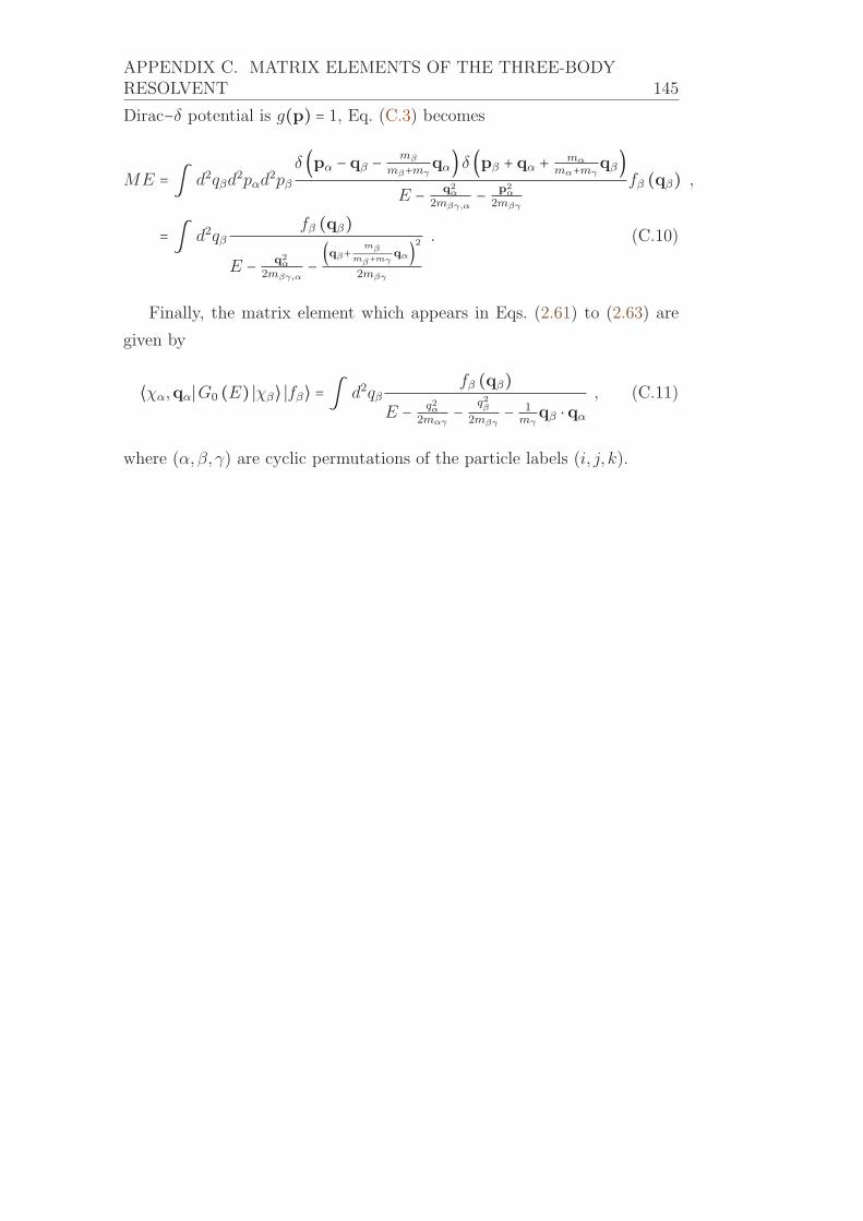
APPENDIX C. MATRIX ELEMENTS OF THE THREE-BODYRESOLVENT 145
Dirac−δ potential is g(p) = 1, Eq. (C.3) becomes
ME = ∫ d2qβd2pαd
2pβδ (pα − qβ −
mβ
mβ+mγqα) δ (pβ + qα +
mα
mα+mγqβ)
E −q2α
2mβγ,α−
p2α
2mβγ
fβ (qβ) ,= ∫ d2qβ
fβ (qβ)E −
q2α
2mβγ,α−
(qβ+ mβ
mβ+mγqα)2
2mβγ
. (C.10)
Finally, the matrix element which appears in Eqs. (2.61) to (2.63) are
given by
⟨χα,qα∣G0 (E) ∣χβ⟩ ∣fβ⟩ = ∫ d2qβfβ (qβ)
E −q2α
2mαγ−
q2β
2mβγ−
1
mγqβ ⋅ qα
, (C.11)
where (α,β, γ) are cyclic permutations of the particle labels (i, j, k).


Appendix D
Numerical methods
The set of integral homogeneous coupled equations in Eq. (2.70) does not
have analytic solution in general and then, it has to be numerically solved.
There are several well established methods available in the literature to
solve integral equations as given, for example, in Ref. [Press 2007]. Besides,
classical techniques as Gauss-Legendre quadratures are used for the numer-
ical discretization of the integral equations, the Newton-Raphson method is
used to find zeros of functions and the Gauss decomposition method is used
to find the determinant of a matrix. Optimized routines which implement
these techniques are available in the libraries of the programming languages
as C, C++ and Fortran and are also described in Ref. [Press 2007].
The three-body problem studied in this thesis consists, basically, of an
eigenvalue - eigenvector problem, where the determination of the energy
(eigenvalue) leads to the determination of the spectator, and consequently,
the wave function (eigenvector).
D.1 Three-body energy (eigenvalue)
In order to illustrate the methods employed in the numerical solution of
Eq. (2.70), the symmetric mass case is considered, i.e., ma = mb = mc = mand Eab = Eac = Ebc = E2. This means that only one integral equation has
to be solved and choosing E2 and m as the energy and mass units, the
three-body energy E3 and the momenta q and k in Eq. (2.70) are rewritten
147

148 D.1. THREE-BODY ENERGY (EIGENVALUE)
as E3 ≡ E3
E2and q ≡ q√
mE2
. In units of E2 =m = 1, Eq. (2.70) becomes
f (q) = 2 ⎡⎢⎢⎢⎢⎣ln⎛⎝√
3
4q2 −E3
⎞⎠⎤⎥⎥⎥⎥⎦−1∫∞
0
dkk f (k)√(−E3 + q2 + k2)2 − (k q)2 , (D.1)
which in a compact form reads
f(q) = ∫ ∞0
K(E3, q, q′)f(q′)dq′ , (D.2)
where k ≡ q′ and the kernel K(E3, q, q′) is defined by
K(E3, q, q′) = 2 ⎡⎢⎢⎢⎢⎣ln
⎛⎝√
3
4q2 −E3
⎞⎠⎤⎥⎥⎥⎥⎦−1
q′√(−E3 + q2 + q′2)2 − (q′ q)2 . (D.3)
The Gauss-Legendre mesh-points are used for the discretization of the
kernel in Eq. (D.3), where the discrete momentum q ≡ xi correspond to
one set of points with the respective Gauss-Legendre weights dq ≡ ωi. The
Gauss-Legendre mesh points and weights are generated, in general, to cal-
culate integrals in the interval [−1,1]. Since the kernel has to be discretized
in the interval [0,∞[, a possible transformation of the set of mesh points
and weights is
qi = 1 + xi1 − xi
wi = 2(1 − xi)2ωi . (D.4)
Therefore, the discretization of the homogeneous integral equation in

APPENDIX D. NUMERICAL METHODS 149
Eq. (D.2) is written as
f(qi) = N
∑j=1
K(E3, qi, qj)f(qj)wj ,
f(qi) − N
∑j=1
K(E3, qi, qj)f(qj)wj = 0 ,(δij − N
∑j=1
K(E3, qi, qj)wj)f(qj) = 0 , (D.5)
where δij is the Kronecker’s delta, 1 ≤ i ≤ N and K(E3, qi, qj) readsK(E3, qi, qj) = 2 ⎡⎢⎢⎢⎢⎣ln
⎛⎝√
3
4q2i −E3
⎞⎠⎤⎥⎥⎥⎥⎦−1
qj√(−E3 + q2
i + q2
j )2 − (qi qj)2 . (D.6)
The matrix form of Eq. (D.5) is given by
HF = 0 (D.7)
whit
H =⎛⎜⎜⎜⎜⎜⎜⎝
1 −K(E3, q1, q1)w1 −K(E3, q1, q2)w2 ⋯ −K(E3, q1, qN)wN
−K(E3, q2, q1)w1 1 −K(E3, q2, q2)w2 ⋯ −K(E3, q2, qN)wN
⋮ ⋮ ⋱ ⋮
−K(E3, qN , q1)w1 −K(E3, qN , q2)w2 ⋯ 1 −K(E3, qN , qN)wN
⎞⎟⎟⎟⎟⎟⎟⎠(D.8)
and
F =⎛⎜⎜⎜⎜⎜⎜⎝
f(q1)f(q2)⋮
f(qN)
⎞⎟⎟⎟⎟⎟⎟⎠. (D.9)
The matrix equation (D.7) only admits non-trivial solution for
detH = det(δij − N
∑j=1
K(E3, qi, qj)wj) = 0 . (D.10)

150 D.1. THREE-BODY ENERGY (EIGENVALUE)
The determinant of H is a function of the three-body energy E3, namely
F (E3) = det(δij − N
∑j=1
K(E3, qi, qj)wj) , (D.11)
and it is calculated, for instance with the Gauss method or the QR-decom-
position [Press 2007]. When E3 corresponds to a three-body bound state
energy, En3, the determinant of H must be null. In other words,
F (En3 ) = 0 , (D.12)
where the superscript n labels the three-body energy for the nth bound
state. which satisfies Eqs. (D.1) and (D.10).
The Newton-Raphson method is used in order to find En3from Eq. (D.11).
Expanding Eq. (D.12) up to first order around E3 gives
F (En3 ) = F (E3) + (En
3 −E3)F ′(E3) = 0 ,En
3 = E3 −F (E3)F ′(E3) , (D.13)
where F ′(E3) = dF (En3)
dEn3
∣En3=E3
. The three-body bound-state energy is found
by successively iterations of Eq. (D.13), where the output of the mth itera-
tion, Em, is used as thin input of the consecutive one. This means that
Em = Em−1 − F (Em−1)F ′(Em−1) for m = 1,2,3... , (D.14)
Notice that an appropriate guess is needed for E0. A good guess can be
found by plotting F (E) vs. E and taking E0 as the point where F (E0) ≈ 0.However, the kernel in Eq. (D.3) presents the so-called well of attraction,
which means that even bad guesses for E0 would lead to the right final
result. The iterative process in Eq. (D.14) must be repeated until
∣Em −Em−1Em−1 ∣ ≤ acc , (D.15)

APPENDIX D. NUMERICAL METHODS 151
where acc is the desired accuracy.
Unfortunately, the functions F and F ′ in Eq. (D.14) does not have an
analytical form. While F (Em) can be easily calculated from Eq. (D.11), its
derivative is found from the definition of derivative
F ′(E) = lim∆E→0
F (E +∆E) − F (E)∆E
, (D.16)
where the discrete version reads
F ′(Em) = F (Em) − F (Em−1)Em −Em−1 , (D.17)
Finally, inserting the derivative (D.17) in Eq. (D.14), the iterative equa-
tion for the three-body energy becomes
Em = Em−1 − F (Em−1) Em−1 −Em−2F (Em−1) − F (Em−2) for m ≥ 2 , (D.18)
where now E1 has also to be guessed. A good try is E1 = 1.1E0.
It is straight forward to extended the method above for the case of three
distinguishable particles, since only the matrix H in Eq. (D.8) and F in
Eq. (D.9) have to be redefined. The set of coupled integral equations is
given in Eq. (2.70). These equations read
fα (q) = 2π⎡⎢⎢⎢⎢⎢⎢⎣4πmβγ ln
⎛⎜⎜⎝¿ÁÁÁÀ q2
2mβγ,α−E3
Eβγ
⎞⎟⎟⎠⎤⎥⎥⎥⎥⎥⎥⎦
−1
×∫∞
0
dk
⎛⎜⎜⎜⎝k fβ (k)√(−E3 +q2
2mαγ+
k2
2mβγ)2 − ( k q
mγ)2
+k fγ (k)√(−E3 +q2
2mαβ+
k2
2mβγ)2 − ( k q
mβ)2⎞⎟⎟⎟⎠ , (D.19)

152 D.1. THREE-BODY ENERGY (EIGENVALUE)
or in a more compact form
fα(q) = ∫ ∞0
Kαβ(E3, q, k)fβ(k)dk +∫ ∞0
Kαγ(E3, q, k)fγ(k)dk , (D.20)
where, writing the labels of each particle explicitly results in three equations,
namely
fa(q) = ∫ ∞0
K12(E3, q, k)fb(k)dk +∫ ∞0
K13(E3, q, k)fc(k)dk , (D.21)
fb(q) = ∫ ∞0
K21(E3, q, k)fa(k)dk +∫ ∞0
K23(E3, q, k)fc(k)dk , (D.22)
fc(q) = ∫ ∞0
K31(E3, q, k)fa(k)dk +∫ ∞0
K32(E3, q, k)fb(k)dk , (D.23)
with the kernels defined as
K12(E3, q, k) =⎡⎢⎢⎢⎢⎢⎣2mbc ln
⎛⎜⎝√
q2
2mbc,a−E3
Ebc
⎞⎟⎠⎤⎥⎥⎥⎥⎥⎦−1k
√(−E3 +q2
2mac+
k2
2mbc)2 − ( k q
mc)2 , (D.24)
K13(E3, q, k) =⎡⎢⎢⎢⎢⎢⎣2mbc ln
⎛⎜⎝√
q2
2mbc,a−E3
Ebc
⎞⎟⎠⎤⎥⎥⎥⎥⎥⎦−1k
√(−E3 +q2
2mab+
k2
2mbc)2 − ( k q
mb)2 , (D.25)
K21(E3, q, k) =⎡⎢⎢⎢⎢⎢⎣2mac ln
⎛⎜⎝√
q2
2mac,b−E3
Eac
⎞⎟⎠⎤⎥⎥⎥⎥⎥⎦−1k
√(−E3 +k2
2mac+
q2
2mbc)2 − ( k q
mc)2 , (D.26)
K23(E3, q, k) =⎡⎢⎢⎢⎢⎢⎣2mac ln
⎛⎜⎝√
q2
2mac,b−E3
Eac
⎞⎟⎠⎤⎥⎥⎥⎥⎥⎦−1k
√(−E3 +q2
2mab+
k2
2mac)2 − ( k q
ma)2 , (D.27)
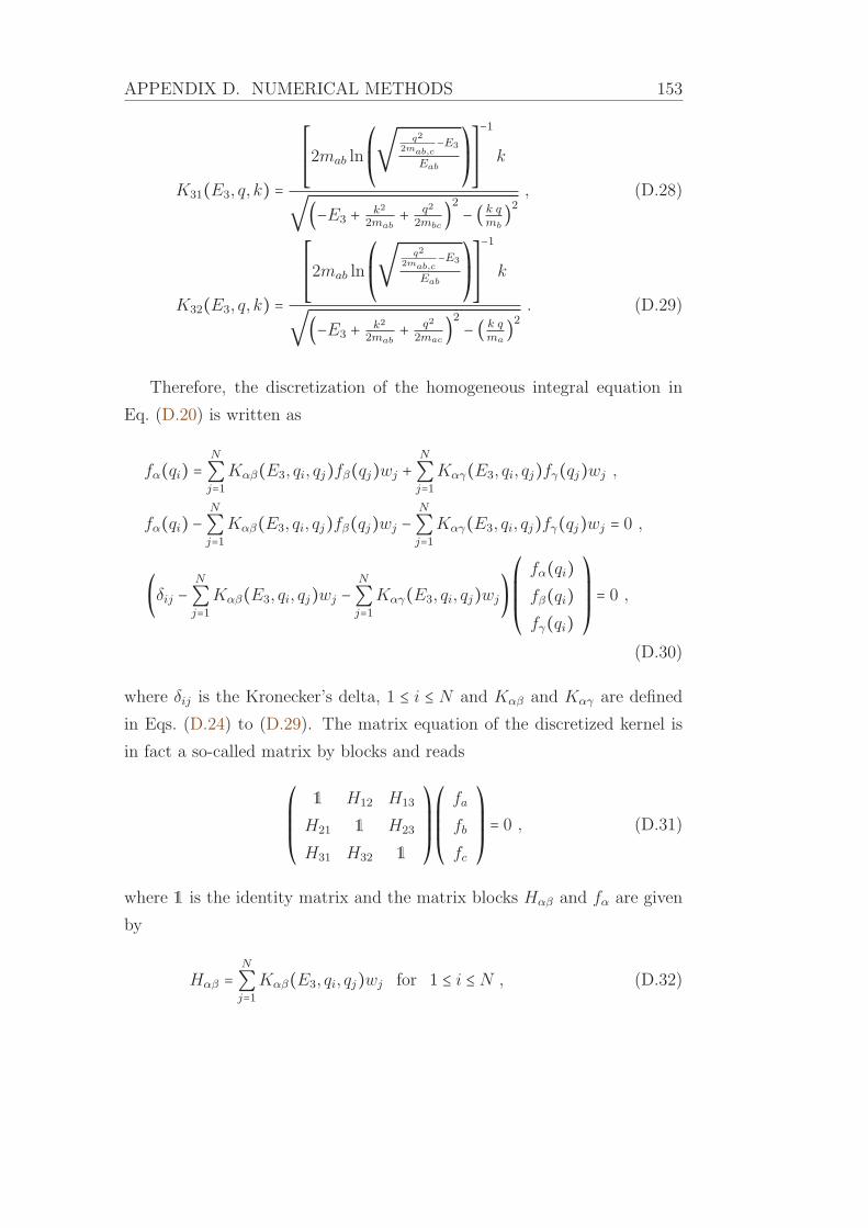
APPENDIX D. NUMERICAL METHODS 153
K31(E3, q, k) =⎡⎢⎢⎢⎢⎢⎣2mab ln
⎛⎜⎝√
q2
2mab,c−E3
Eab
⎞⎟⎠⎤⎥⎥⎥⎥⎥⎦−1k
√(−E3 +k2
2mab+
q2
2mbc)2 − ( k q
mb)2 , (D.28)
K32(E3, q, k) =⎡⎢⎢⎢⎢⎢⎣2mab ln
⎛⎜⎝√
q2
2mab,c−E3
Eab
⎞⎟⎠⎤⎥⎥⎥⎥⎥⎦−1k
√(−E3 +k2
2mab+
q2
2mac)2 − ( k q
ma)2 . (D.29)
Therefore, the discretization of the homogeneous integral equation in
Eq. (D.20) is written as
fα(qi) = N
∑j=1
Kαβ(E3, qi, qj)fβ(qj)wj +
N
∑j=1
Kαγ(E3, qi, qj)fγ(qj)wj ,
fα(qi) − N
∑j=1
Kαβ(E3, qi, qj)fβ(qj)wj −
N
∑j=1
Kαγ(E3, qi, qj)fγ(qj)wj = 0 ,
(δij − N
∑j=1
Kαβ(E3, qi, qj)wj −
N
∑j=1
Kαγ(E3, qi, qj)wj)⎛⎜⎜⎜⎝fα(qi)fβ(qi)fγ(qi)
⎞⎟⎟⎟⎠ = 0 ,(D.30)
where δij is the Kronecker’s delta, 1 ≤ i ≤ N and Kαβ and Kαγ are defined
in Eqs. (D.24) to (D.29). The matrix equation of the discretized kernel is
in fact a so-called matrix by blocks and reads
⎛⎜⎜⎜⎝1 H12 H13
H21 1 H23
H31 H32 1
⎞⎟⎟⎟⎠⎛⎜⎜⎜⎝fa
fb
fc
⎞⎟⎟⎟⎠ = 0 , (D.31)
where 1 is the identity matrix and the matrix blocks Hαβ and fα are given
by
Hαβ = N
∑j=1
Kαβ(E3, qi, qj)wj for 1 ≤ i ≤ N , (D.32)

154 D.2. SPECTATOR FUNCTIONS (EIGENVECTOR)
fα = fα(qi) for 1 ≤ i ≤ N . (D.33)
Or, in matrix form
fα =⎛⎜⎜⎜⎜⎜⎜⎝
fα(q1)fα(q2)⋮
fα(qN)
⎞⎟⎟⎟⎟⎟⎟⎠(D.34)
and, in the same way, the matrix blocks Hαβ are
Hαβ =⎛⎜⎜⎜⎜⎜⎜⎝
Kαβ(E3, q1, q1)w1 Kαβ(E3, q1,12)w2 ⋯ Kαβ(E3, q1, qN)wN
Kαβ(E3, q2, q1)w1 Kαβ(E3, q2, q2)w2 ⋯ Kαβ(E3, q2, qN)wN
⋮ ⋮ ⋱ ⋮
Kαβ(E3, qN , q1)w1 Kαβ(E3, qN , q2)w2 ⋯ Kαβ(E3, qN , qN)wN
⎞⎟⎟⎟⎟⎟⎟⎠.
(D.35)
Finally, Eq. (D.31) can be written as Eq. (D.7), i.e., HF = 0 and the
steps between Eqs. (D.10) and (D.18) are the same, giving the three-body
energy for a system composed for three-distinguishable particles.
D.2 Spectator functions (eigenvector)
The method is illustrated for the case of identical particles, since it allows a
simpler notation. However, the procedure is general and easily extended to
the case of three-distinguishable particles, as it was done in the calculation
of the three-body energy in Sec. D.1.
Once the three-bode energy E3 is calculated, it should be inserted again
in Eq. (D.5) in order to once more generate the matrix H, as given in
Eq. (D.8). Now, the matrix equation HF = 0 (see Eq. (D.7)) is simply a set
of N equations for N unknown, namely, each value of the spectator function
f(qn) has to be determined in a point qn, with 1 ≤ n ≤ N .
The set of N equations is given by
N
∑j=1
Hij(E3, qi, qj)f(qj) = 0 for 1 ≤ i ≤ N . (D.36)

APPENDIX D. NUMERICAL METHODS 155
Notice, however, that the three-body energy calculated in the last section
is the one which fulfills detH = 0. This means that one of the equations
from the set is redundant and that the system in Eq. (D.36) can not be
unequivocally determined. In other words, N − 1 variables will be given in
terms of an arbitrary value. This freedom in the system is utilized to set,
for instance, f(q1) = 1. Then, eliminating a line and a column in Eq.(D.7),
the system of equations becomes
N
∑j=2
Hij(E3, qi, qj)f(qj) = −Hi1f(q1) = −Hi1 for 2 ≤ i ≤ N , (D.37)
or in the matrix form
H(N−1)x(N−1)
✎
✍
☞
✌
✎
✍
☞
✌
1
f(q2)
⋮
⋮
⋮
f(qN)
= 0 ,
where all the unknown f(qn) with 2 ≤ n ≤ N are determined in term of
f(q1) = 1. There is no problem in choosing an arbitrary value for f(q1),since the wave-function is defined unless a normalization constant. The
Gauss-Jordan elimination method in then used to solve the set algebraic
equations in Eq. (D.37). Besides, this method still holds in the case of
three-distinguishable particles, where the only difference arises from the
matrix H and F which have to be respectively defined as in Eqs. (D.32)
and (D.33), whose matrix form is given in Eq. (D.31).


Appendix E
Asymptotic one-body density
in 3D
The large momentum limit of the four terms in Eqs. (6.25) to (6.28) is
worked out in this Appendix.
E.0.1 Asymptotic contribution from n1(qB)As in the 2D case, this is also the simplest term. The asymptotic form of the
spectator function from Eq. (6.17) is inserted in Eq. (6.25), the first out of
the four terms of the momentum distribution. Taking the large momentum
limit results in
n1(qB)→ 2π2
√ AA + 2 ∣χAA(qB)∣2qB
→ 2π2 ∣cAA∣2√ AA + 2 ∣sin(s ln qB/q∗)∣2
q5B,
→ π2
q5B∣cAA∣2
√ AA + 2 , (E.1)
where the 1/2 came from the average of the oscillating part.
E.0.2 Asymptotic contribution from n2(qB)For large qB, Eq. (6.26) becomes
n2(qB) =2∫ d3qA∣χAB(qA)∣2(q2A + qA ⋅ qB + q
2
BA+12A )2 ,
= 8A2
q4B (A + 1)2 ∫ d3qA ∣χAB(qA)∣2 + n2s(qB) , (E.2)
157

158
where a sub-leading part, n2s(qB), is retained since it is of the same order
as the leading order of the other terms. It is important to emphasize that
the one-body large-momentum leading order comes only from n2(qB). Thespectator function can not be replaced by its asymptotic expression, because
the main contribution to ∫ ∞0 dqA q2
A ∣χAB(qA)∣2 arises from small qA. This
replacement would therefore lead to a completely wrong result. However,
this is not always the case, as shown below for n2s(qB).The sub-leading term is
n2s(qB) = ∫ d3qA ∣χAB(qA)∣2 ⎡⎢⎢⎢⎢⎣2
(q2A + qA ⋅ qB + q2
BA+12A )2 −
8A2
(A + 1)2 1
q4B
⎤⎥⎥⎥⎥⎦ ,= ∣cAB ∣2∫ d3qA
q4A
⎡⎢⎢⎢⎢⎣1
(q2A + qA ⋅ qB + q2
BA+12A )2 −
4A2
(A + 1)2 1
q4B
⎤⎥⎥⎥⎥⎦ ,= 2π ∣cAB ∣2
q5B∫∞−∞
dx
x2[ 1
x4 + 1Ax2 + (A+12A )2 −1(A+1
2A )2 ] , (E.3)
where it was used in the second line the asymptotic form of ∣χAB(qA)∣2 =∣cAB ∣3q−4A /2 obtained after averaging over the oscillatory term in Eq. (6.17).
Next, the angular integral was solved and the variable qA = qBx introduced.
Since the integrand is even the integration can be extended to the entire
real axis.
The function under the integral,
f(x) = 1
x2[ 1
x4 + 1Ax2 + (A+12A )2 −1(A+1
2A )2 ] , (E.4)
falls off faster than 1/x for ∣x∣→∞. Therefore, it is extended to the complex
domain, where a contour in the upper-half plane that includes the real
axis and a semi-circle of large radius in a counterclockwise orientation is
considered. The poles of f(x) have to be determined in order to use the
Cauchy residue theorem. Since f(x) is regular at x = 0, the four poles are

APPENDIX E. ASYMPTOTIC ONE-BODY DENSITY IN 3D 159
out in the complex plane and are given by
x1 = reiθ1/2, x2 = rei(π−θ1/2), x3 = rei(π+θ1/2), x4 = re−iθ1/2, (E.5)
where r = √A+12A and tan2 θ1 = A(A + 2). Following the convention from
Eqs. (6.19) to (6.21), where π/2 < θ1 < π, then x1 and x2 are the poles in
the upper-half plane. The sum of the two residues is
Res(f, x1) +Res(f, x2) = − 1
ir3A(A + 3)(A + 1)2 cos(θ1
2)
sin(θ1) . (E.6)
Using the residue theorem, the sub-leading term in Eq. (E.3) becomes
n2s(qB) = − 4π2 ∣cAB ∣2q5B2 sin(θ12 )
A(A + 3)(A + 1)2 ( 2AA + 1)3/2
, (E.7)
where, from the definition of θ1, cosθ1 = − 1A+1 and [2 sin(θ12)]−1 =√ A+1
2(A+2) .Finally, the sub-leading term in n2 is given by
⟨n2(qB)⟩ = −8π2 ∣cAB ∣2q5B
A3(A + 3)(A + 1)3√A(A + 2) , (E.8)
where the special case A = 1 yields ⟨n2(qB)⟩ = −4π2 ∣cAB ∣2 /(√3q5B). The
sub-index s was dropped, since this term has the same order as the leading-
order of the n3(qB) and n4(qB) terms.
E.0.3 Asymptotic contribution from n3(qB)
The structure of n3(qB) in Eq. (6.27) is similar to n2(qB) in Eq. (6.26). The
only difference is that the spectator function under the integration sign is
not squared anymore. This small functional difference leads to a completely
different result. Neglecting the three-body energy and changing variables

160
to qA = pB −qB
2in Eq. (6.27) results in
n3(qB) = 2χ∗AA(qB)∫ d3qAχAB(qA)(q2A + q2B A+12A + qA ⋅ qB)2 + c.c. ,
= 2χ∗AA(qB)∫ d3y q3BχAB(qB y)(y2q2B + q2B A+12A + yq2B cos θ)2 + c.c. ,
= 2χ∗AA(qB)qB
∫ d3yχAB(qB y)(y2 + A+1
2A + y cos θ)2 + c.c. ,= 4πχ∗AA(qB)
qB∫∞
0
dy y2∫π
0
dθ sin θχAB(qB y)(y2 + A+12A + y cos θ)2 + c.c. . (E.9)
where in the second line it was defined qA = qBy.
The angular integral is
∫π
0
dθ sin θ
(y2 + A+12A + y cos θ)2 = ∫
1
−1dx(A +Bx)2 = −1B ∫
A+BA−B
dz
z2= −1B
1
z∣A+BA−B ,
= 2
A2 −B2= 2
(y2 + A+12A )2 − y2 ,
= 2
y4 + 1Ay2 + (A+12A )2 . (E.10)
Besides, replacing the spectator functions χAA and χAB by their asymptotic
form, as given in Eq. (6.17), results in
χ∗AA(qB) = c∗AA
q2Bsin(s ln qB
q∗ ) , (E.11)
χAB(qB y) = cAB
y2 q2Bsin [s ln(qB y
q∗ )] ,= cAB
y2 q2Bsin(s ln qB
q∗ + s ln y) ,= cAB
y2 q2B[sin(s ln qB
q∗ ) cos (s ln y) + sin (s ln y) cos(s ln qBq∗ )] .(E.12)

APPENDIX E. ASYMPTOTIC ONE-BODY DENSITY IN 3D 161
Inserting Eqs. (E.10) to (E.12) into Eq. (E.9) gives
n3(qB) = 8πc∗AA cAB
q5Bsin2(s ln qB/q∗)∫ ∞
0
cos(s ln y) dyy4 + 1Ay2 + (A+12A )2
+ 8πc∗AA cAB
q5Bsin(s ln qB/q∗) cos(s ln qB/q∗)∫ ∞
0
sin(s ln y) dyy4 + 1Ay2 + (A+12A )2 + c.c. .
(E.13)
Averaging out the oscillatory terms, only the first term of Eq. (E.13) gives
a non-vanishing result
⟨n3(qB)⟩ = 4πc∗AA cAB
q5B∫∞
0
cos(s ln y) dyy4 + 1Ay2 + (A+12A )2 + c.c. . (E.14)
Expressing cosine in the complex exponential form
cos(s ln y) = eıs ln y + e−ıs ln y
2= eln yıs + eln y−ıs
2= yıs + y−ıs
2, (E.15)
the integral in Eq. (E.14) becomes
I(s) = ∫ ∞0
cos(s ln y) dyy4 + 1Ay2 + (A+12A )2 =
1
2 ∫∞
0
dyyıs + y−ıs
y4 + 1Ay2 + (A+12A )2 . (E.16)
In order to extended the integration to the full real axis, the variables are
changed to y = eα, where dy = eαdα and the integral I(s) is expressed as
I(s) = 1
2 ∫∞−∞
dα eα (eısα + e−ısα)e4α + 1Ae2α + (A+12A )2 = Re Iα(s) , (E.17)
where Re denotes the real part and the integral Iα(s) is explicitly rewritten
in terms of its poles as
Iα(s) = ∫ ∞−∞
eα(1+ıs) dα(eα − eα1) (eα − eα2) (eα − eα3) (eα − eα4) . (E.18)
The integral (E.17) is solved using the residues theorem. The next steps are

162
about finding the poles of the integrand f(α) and evaluating the residues
of the poles. In order to simplify the calculation of the roots in the de-
nominator of f(α), the variable x = y2 = e2α is introduced. The zeros of
the denominator in Eq. (E.17) are found from x2 + 1Ax + (A+12A )2 = 0 and are
given by
x± = − 1
2A ± 1
2
√1A2− (A + 1
2A )2 = 1
2A (−1 ± ı√A(A + 2)) . (E.19)
In the variable y = ±√x these roots read
y1 = +√
1
2A (−1 + ı√A(A + 2))1/2 = +1
2+ ı
√A + 24A = reıθ3 , (E.20)
y2 = −√
1
2A (−1 + ı√A(A + 2))1/2 = −1
2− ı
√A + 24A = re−ı(π−θ3) = −reıθ3 ,
(E.21)
y3 = +√
1
2A (−1 − ı√A(A + 2))1/2 = +1
2− ı
√A + 24A = re−ıθ3 , (E.22)
y4 = −√
1
2A (−1 − ı√A(A + 2))1/2 = −1
2+ ı
√A + 24A = reı(π−θ3) = −re−ıθ3 .
(E.23)
Finally, the roots in the variable α = ln y are
α1 = ln y1 = ln r + ıθ3 , (E.24)
α2 = ln y2 = ln r − ı(π − θ3) , (E.25)
α3 = ln y3 = ln r − ıθ3 , (E.26)
α4 = ln y4 = ln r + ı(π − θ3) , (E.27)
showing that all of them are in the complex plane, out of the real axis. The
quantities r and θ3 are defined as
r =√A + 1
2A , (E.28)

APPENDIX E. ASYMPTOTIC ONE-BODY DENSITY IN 3D 163
tan θ3 =√A + 2A for 0 ≤ θ3 ≤ π
2. (E.29)
A rectangle of vertices −R, +R, +R+ ıπ and −R+ ıπ molds a closed path in
a complex plane, as shown in Fig. E.1. Due to the restriction of θ3, given in
Eq. (E.29), this closed path encompasses the poles α1 and α4 in the upper-
half plane and then, four integrals have to be worked out, namely J1 which
extends along the real axis from −R to +R, J2 from +R to +R+ ıπ, J3 from
+R + ıπ to −R + ıπ and J4 from −R + ıπ to −R.
Figure E.1: A rectangle of vertices −R, +R, +R + ıπ and −R + ıπ, whichmolds the closed path in a complex plane of z. The poles α1 and α4 areencompassed in the upper-half plane. The the direction of integration ofthe four integrals J1, J2, J3 and J4 are indicated by the arrows.
The residues theorem is used to calculate Iα(s). The integral in the
closed path reads
∮ dz ez eısz
e4z + 1Ae2z + (A+12A )2 = J1 + J2 + J3 + J4 = 2πı[Res(f,α1) +Res(f,α4)] ,(E.30)

164
where changing variables to the z = α + ı 0, the integral J1 reads
J1 = limR→∞∫
R
−Rdα eα eısα
e4α + 1Ae2α + (A+12A )2 → Iα(s) . (E.31)
Analogously, setting z = R + ı y gives dz = ı dy and the integral J2 becomes
J2 = limR→∞∫
R+ıπR
dz ez eısz
e4z + 1Ae2z + (A+12A )2 ,= lim
R→∞ ı∫π
0
dy eR+ıy eıs(R+ıy)e4(R+ıy) + 1Ae2(R+ıy) + (A+12A )2 ,
= limR→∞
eR
e4Rı∫
π
0
dy eıy eıs(R+ıy)e4ıy + Ae2ıy 1
e2R+ (A+1
2A )2 1
e4R
→ 0 . (E.32)
The integral J3 is similar to J1 and changing variables to z = α+ ıπ it reads
J3 = limR→∞∫
−R+ıπR+ıπ
dz ez eısz
e4z + 1Ae2z + (A+12A )2 ,= lim
R→∞∫−R
R
dα eα+ıπ eıs(α+ıπ)e4(α+ıπ) + 1Ae2(α+ıπ) + (A+12A )2 ,
= limR→∞∫
R
−Rdα eα eısαe−sπ
e4α + 1Ae2α + (A+12A )2 → e−sπJ1 = e−sπIα(s) , (E.33)
where eα+ıπ = eαeıπ = −eα. Then, performing the same transformation as in
J2, the last term becomes
J4 = limR→∞∫
−R−R+ıπ
dα eα eısα
e4α + 1Ae2α + (A+12A )2 ,= lim
R→∞ ı∫0
π
dy eR+ıy eıs(R+ıy)e4(R+ıy) + 1Ae2(R+ıy) + (A+12A )2 ,= − lim
R→∞J2 → 0 , (E.34)
Summarizing, in the limit R → ∞, the integrals are J1 = Iα(s), J3 =

APPENDIX E. ASYMPTOTIC ONE-BODY DENSITY IN 3D 165
e−sπIα(s) and J2, J4 → 0. Then, from Eq. (E.30) the integral Iα(s) readsIα(s) = 2πı
1 + e−πs [Res(f,α1) +Res(f,α4)] . (E.35)
In order to calculate the residues of the poles α1 and α4, it is necessary to
expand the nth root, in the limit α → αn, as
eα − eαn = eα (1 − eαn−α) = eα (1 − 1 − (αn − α) − (αn − α)22!
− ...) ,= eα (α − αn) (1 + (α − αn)
2!− ...) . (E.36)
Besides, notice that the exponential of each root αn in Eqs. (E.24) to (E.27)
is already given in Eqs. (E.20) to (E.23). Taking the first order in the
expansion, the residues are given by
Res(f,α1) = limα→α1
(α − α1) eα(1+ıs)eα (α − α1) (eα − eα2) (eα − eα3) (eα − eα4) ,
= eα1 eısα1
eα1 (eα1 − eα2) (eα1 − eα3) (eα1 − eα4) ,= eısα1
8ır3 sin θ3 cos θ3eıθ3,
= 1
2ı
√ AA + 2 1
cos θ3eıs(ln r+ıθ3)−ıθ3 , (E.37)
and
Res(f,α4) = limα→α4
(α − α4) eα(1+ıs)eα (α − α4) (eα − eα1) (eα − eα2) (eα − eα3) ,
= eα4 eısα4
eα4 (eα4 − eα1) (eα4 − eα2) (eα4 − eα3) ,= eısα4
8ır3 sin θ3 cos θ3e−ıθ3 ,
= 1
2ı
√ AA + 2 1
cos θ3eıs[ln r+ı(π−θ3)]+ıθ3 , (E.38)
Inserting the residues of the poles from Eqs. (E.37) and (E.38) into

166
Eq. (E.35) gives
Iα(s) = π
1 + e−πs√ AA + 2 1
cos θ3(eıs(ln r+ıθ3)−ıθ3 + eıs[ln r+ı(π−θ3)]+ıθ3) ,
= 2πe−sπ/21 + e−πs
√ AA + 2 1
cos θ3eıs ln r cosh [s(θ3 − π
2) + ıθ3] ,
= π
cosh (sπ2)√ AA + 2 1
cos θ3[cos (s ln r) + ı sin (s ln r)]
× {cos θ3 cosh [s(π2− θ3)] − ı sin θ3 sinh [s(π
2− θ3)]} ,
= π
cosh (sπ2)√ AA + 2 1
cos θ3
× {cos θ3 cos (s ln r) cosh [s(π2− θ3)]
+ sin θ3 sin (s ln r) sinh [s(π2− θ3)]}
× −ı{sin θ3 cos (s ln r) sinh [s(π2− θ3)]
+ cos θ3 sin (s ln r) cosh [s(π2− θ3)]} ,
= π
cosh (sπ2){√ AA + 2 cos (s ln r) cosh [s(π2 − θ3)]
+ sin (s ln r) sinh [s(π2− θ3)]}
× −ı{cos (s ln r) sinh [s(π2− θ3)]
+
√ AA + 2 sin (s ln r) cosh [s(π2 − θ3)]} , (E.39)
where the the real, Re, and imaginary, Im, parts of Iα(s) are explicitly given
by
Re Iα(s) = π
cosh ( sπ2)⎧⎪⎪⎨⎪⎪⎩√ AA + 2 cos (s ln r) cosh [s(π2 − θ3)]
+ sin (s ln r) sinh [s(π2− θ3)]} , (E.40)

APPENDIX E. ASYMPTOTIC ONE-BODY DENSITY IN 3D 167
Im Iα(s) = −π
cosh ( sπ2)⎧⎪⎪⎨⎪⎪⎩√ AA + 2 sin (s ln r) cosh [s(π2 − θ3)]
+ cos (s ln r) sinh [s(π2− θ3)]} , (E.41)
with r and θ3 defined respectively in Eqs. (E.28) and (E.29).
Finally, from equations (E.14), (E.17) and (E.40), the non-oscillating
part of n3(qB) is given by
⟨n3(qB)⟩ = 4π2cAA cAB
q5B cosh ( sπ2)⎧⎪⎪⎨⎪⎪⎩√ AA + 2 cos⎛⎝s ln
√A + 12A ⎞⎠ cosh [s(π2 − θ3)]
+ sin⎛⎝s ln
√A + 12A ⎞⎠ sinh [s(π2 − θ3)]
⎫⎪⎪⎬⎪⎪⎭ , (E.42)
where tan θ3 =√A+2A for 0 ≤ θ3 ≤ π/2. The special case A = 1 yields θ3 = π/3and ⟨n3(qB)⟩ = 4π2∣cAA∣2 cosh ( sπ6 ) / (q5B√3 cosh ( sπ2 )).
E.0.4 Asymptotic contribution from n4(qB)
As in the 2D case, this is also the most complicated out of the four additive
terms in the one-body momentum density, since the angular dependence in
both spectator arguments of Eq. (6.28) can not be removed simultaneously
by a change in variables. Then, although Eqs. (6.27) and (6.28) are similar,
it is not possible to extend the results from the previous case, n3(qB), toobtain the non-oscillating part of n4(qB). Defining pB = qB
2y and dropping
the three-body energy, Eq. (6.28) becomes
n4(qB) = 4π
qB∫∞
0
y2dy
(y2 + A+2A )2 ∫+1−1 dx χ∗AB(qBx−)χAB(qBx+) + c.c. , (E.43)

168
where x± = 1
2
√1 + y2 ± 2yx. The asymptotic spectator function for a shifted
argument is given in Eq. (E.12) and χAB(qBx±) readsχAB(qB x±) = cAB
x2± q2B[sin(s ln qB
q∗ ) cos (s lnx±) + sin (s lnx±) cos(s ln qBq∗ )] .(E.44)
The spectator function in Eq. (E.43) are replaced by their asymptotic
form from Eq. (E.44). The integral is then separated in three terms, namely
n4(qB) = 8π∣cAB ∣2 sin2 (s ln qBq∗)
q5B
×∫∞
0
y2dy
(y2 + A+2A )2 ∫+1−1
dx
x2+x2−cos (s lnx+) cos (s lnx−)
+
8π∣cAB ∣2 cos2 (s ln qBq∗)
q5B
×∫∞
0
y2dy
(y2 + A+2A )2 ∫+1−1
dx
x2+x2−sin (s lnx+) sin (s lnx−)
+
4π∣cAB ∣2 sin (s ln qBq∗) cos (s ln qB
q∗)
q5B
×∫∞
0
y2dy
(y2 + A+2A )2 ∫+1−1
dx
x2+x2−sin [s ln (x+x−)] . (E.45)
As it was done for n3(qB), averaging out the oscillatory term, only the
two first terms on the right-hand-side of Eq. (E.45) give a non-vanishing
contribution. The angular integration is performed using that
∫ dx(β + xβ − x
)±ıs/2 (β2− x2)−1 = ±(β + x
β − x)±ıs/2 (ıβs)−1 . (E.46)
Then, the angular part of Eq. (E.45) has to be written as Eq. (E.46). The
denominator in the integrand of the first two terms on the right hand side
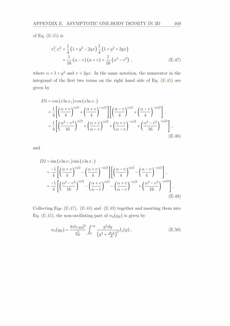
APPENDIX E. ASYMPTOTIC ONE-BODY DENSITY IN 3D 169
of Eq. (E.45) is
x2+ x2− = 1
4(1 + y2 − 2yx) 1
4(1 + y2 + 2yx)
= 1
16(α − v) (α + v) = 1
16(α2− v2) , (E.47)
where α = 1 + y2 and v = 2yx. In the same notation, the numerator in the
integrand of the first two terms on the right hand side of Eq. (E.45) are
given by
D1 = cos (s lnx+) cos (s lnx−)= 1
4[(α + v
4)ıs/2 + (α + v
4)−ıs/2] [(α − v
4)ıs/2 + (α − v
4)−ıs/2] ,
= 1
4[(α2 − v2
16)ıs/2 + (α + v
α − v)ıs/2 + (α + v
α − v)−ıs/2 + (α2 − v2
16)−ıs/2] ,
(E.48)
and
D2 = sin (s lnx+) sin (s lnx−)= −1
4[(α + v
4)ıs/2 − (α + v
4)−ıs/2] [(α − v
4)ıs/2 − (α − v
4)−ıs/2] ,
= −14[(α2 − v2
16)ıs/2 − (α + v
α − v)ıs/2 − (α + v
α − v)−ıs/2 + (α2 − v2
16)−ıs/2] .
(E.49)
Collecting Eqs. (E.47), (E.48) and (E.49) together and inserting them into
Eq. (E.45), the non-oscillating part of n4(qB) is given by
n4(qB) = 4π∣cAB ∣2q5B
∫∞
0
y2dy
(y2 + A+2A )2 Ix(y) , (E.50)

170
where the angular integral Ix(y) readsIx(y) = ∫ +1
−1dx
x2+x2−[cos (s lnx+) cos (s lnx−) + sin (s lnx+) sin (s lnx−)] ,
= ∫ +1−1
dx
2[(1 + y2 + 2yx
1 + y2 − 2yx)ıs/2 + (1 + y2 + 2yx
1 + y2 − 2yx)−ıs/2] 16(1 + y2)2 − 4x2y2 ,
= 8
4y2 ∫+1−1 dx
⎡⎢⎢⎢⎢⎢⎣⎛⎝
1+y22y+ x
1+y22y− x
⎞⎠ıs/2
+⎛⎝
1+y22y− x
1+y22y− x
⎞⎠−ıs/2⎤⎥⎥⎥⎥⎥⎦
[(1 + y22y)2 − x2]−1 ,
(E.51)
which looks like the expression in Eq. (E.46). Then, the result is
Ix(y) = 2
y22y
ıs(1 + y2)⎧⎪⎪⎪⎪⎨⎪⎪⎪⎪⎩⎡⎢⎢⎢⎢⎢⎣⎛⎝
1+y22y+ x
1+y22y− x
⎞⎠ıs/2⎤⎥⎥⎥⎥⎥⎦RRRRRRRRRRRRRR1
x=−1−
⎡⎢⎢⎢⎢⎢⎣⎛⎝
1+y22y+ x
1+y22y− x
⎞⎠−ıs/2⎤⎥⎥⎥⎥⎥⎦
RRRRRRRRRRRRRR1
x=−1
⎫⎪⎪⎪⎪⎬⎪⎪⎪⎪⎭,
= 8
ısy(1 + y2)⎡⎢⎢⎢⎢⎢⎣⎛⎝
1+y22y+ 1
1+y22y− 1
⎞⎠ıs/2
−⎛⎝
1+y22y+ 1
1+y22y− 1
⎞⎠−ıs/2⎤⎥⎥⎥⎥⎥⎦
,
= 8
ısy(1 + y2)⎡⎢⎢⎢⎢⎢⎣⎛⎜⎝¿ÁÁÀ(y + 1)2(y − 1)2
⎞⎟⎠ıs
−
⎛⎜⎝¿ÁÁÀ(y + 1)2(y − 1)2
⎞⎟⎠−ıs⎤⎥⎥⎥⎥⎥⎦
. (E.52)
Combining the expressions in Eqs. (E.50) and (E.52), the non-oscillating
part of n4(qB) reads⟨n4(qB)⟩ = 32π∣cAB ∣2
ı s q5B∫∞
0
y dy
(y2 + A+2A )2 (1 + y2) [(y + 1∣y − 1∣)
ıs
− ( y + 1∣y − 1∣)−ıs] ,
= 64π∣cAB ∣2s q5B
∫∞
0
y dy
(y2 + A+2A )2 (1 + y2) sin(s ln(y + 1∣y − 1∣)) , (E.53)
however the absolute value complicates the calculation of the integral. Cir-
cumventing this problem, the integral is split in two pieces: y ∈ [0,1] andy ∈ [ 1,∞ [ and a new variable is introduced in each piece, i.e., the variable
transformation y = x−1x+1 is made in the first piece and y = x+1
x−1 in the second

APPENDIX E. ASYMPTOTIC ONE-BODY DENSITY IN 3D 171
one [Castin 2011]. Notice that in both cases x ∈ [1,∞[. In detail
⟨n4(qB)⟩ = 64π∣cAB ∣2s q5B
[I<(s) + I>(s)] , (E.54)
where
I<(s) = ∫ 1
0
y dy
(y2 + A+2A )2 (1 + y2) sin(s ln(y + 1∣y − 1∣)) ,
= ∫ ∞1
2 dx(x + 1)2 x − 1x + 1sin (s lnx)/⎧⎪⎪⎨⎪⎪⎩[(
x − 1
x + 1)2 + A + 2A ]2 [(x − 1
x + 1)2 + 1]⎫⎪⎪⎬⎪⎪⎭ ,
= ∫ ∞1
2(x − 1) dx(x + 1)3 sin (s lnx) (x + 1)6[(A+2A + 1) (x2 + 1) + (A+2A − 1)2x]2 2 (x2 + 1) ,
= ∫ ∞1
dx(x − 1)(x + 1)3 sin (s lnx)
[ 2A (A + 1) (x2 + 1) + 4Ax]2 (x2 + 1) , (E.55)
and
I>(s) = ∫ ∞1
y dy
(y2 + A+2A )2 (1 + y2) sin(s ln(y + 1∣y − 1∣)) ,
= −∫ 1
∞2 dx(x − 1)2 x + 1x − 1
sin (s lnx)/⎧⎪⎪⎨⎪⎪⎩[(x + 1
x − 1)2 + A + 2A ]2 [(x + 1
x − 1)2 + 1]⎫⎪⎪⎬⎪⎪⎭ ,
= ∫ ∞1
2(x + 1) dx(x − 1)3 sin (s lnx) (x − 1)6[(A+2A + 1) (x2 + 1) − (A+2A − 1)2x]2 2 (x2 + 1) ,
= ∫ ∞1
dx(x + 1)(x − 1)3 sin (s lnx)
[ 2A (A + 1) (x2 + 1) − 4Ax]2 (x2 + 1) . (E.56)
The sum of the two integrals in Eqs. (E.55) and (E.56), I+(s), is found to
be
I+(s) = ∫ ∞1
dx(x + 1)(x − 1) sin (s lnx)
x2 + 1
×
⎧⎪⎪⎨⎪⎪⎩(x + 1)2
[ 2A (A + 1) (x2 + 1) + 4Ax]2 +(x − 1)2
[ 2A (A + 1) (x2 + 1) − 4Ax]2⎫⎪⎪⎬⎪⎪⎭ ,

172
= 16A2 ∫∞
1
dx sin (s lnx) x2 − 1x2 + 1
×
2 (x2 + 1) [ (A+1)24
x4 + ( (A+1)22+ 1)x2 + 1] + 4x[(A + 1) (x3 + x)]
[ 4A2 (A + 1)2 (x2 + 1)2 − 16A2x2]2 ,
= A2∫∞
1
dx sin (s lnx) x2 − 1x2 + 1
×
(A+1)22
x6 + (32A2 + 7A + 15
2) + (A + 3)2 x2 + 2
{(A + 1)2 x4 + [2 (A2 + 1)2 − 4]x2 + (A2 + 1)2}2 ,= A2
2 (A + 1)4 ∫∞
1
dx sin (s lnx) x2 − 1x2 + 1
×(A + 1)2 (x6 + 1) + (3A2 − 2A − 1) (x4 + x2)
[x4 + (2 − 4
(A+1)2)x2 + 1]2.
(E.57)
From Eq. (E.54), ⟨n4(qB)⟩ becomes
⟨n4(qB)⟩ = 32π∣cAB ∣2s q5B
A2
(A + 1)4×∫
∞1
dx sin (s lnx) x2 − 1x2 + 1
(A + 1)2 (x6 + 1) + (3A2 − 2A − 1) (x4 + x2)[x4 + (2 − 4
(A+1)2)x2 + 1]2.
(E.58)
The residue theorem is used to calculate the non-oscillating part of
n4(qB). The poles of Eq. (E.58) are given by
x1 = 1A + 1 (1 + ı√A (A + 1)) =
¿ÁÁÀ1 +A2 + 2A(A + 1)2 eıθ4 = eıθ4 , (E.59)
x2 = 1A + 1 (−1 + ı√A (A + 1)) = eı(π−θ4) = −e−ıθ4 , (E.60)
x3 = 1A + 1 (1 − ı√A (A + 1)) = e−ıθ4 , (E.61)
x4 = 1A + 1 (−1 − ı√A (A + 1)) = e−ı(π−θ4) = −eıθ4 , (E.62)
x5 = ı = eıπ2 , (E.63)

APPENDIX E. ASYMPTOTIC ONE-BODY DENSITY IN 3D 173
x6 = −ı = e−ıπ2 , (E.64)
with
tan θ4 =√A(A + 2) for 0 ≤ θ4 ≤ π2. (E.65)
Notice that the roots xn with 1 ≤ n ≤ 4 are of order two. Changing variables
to x = eα, the domain of integration is now to the entire real axis, namely
⟨n4(qB)⟩ = 32π∣cAB ∣2s q5B
A2
(A + 1)4 ∫∞
0
dαeα sin (s α) e2α − 1e2α + 1
×(A + 1)2 (e6α + 1) + (3A2 − 2A − 1) (e4α + e2α)
[e4α + (2 − 4
(A+1)2) e2α + 1]2,
= 16π∣cAB ∣2s q5B
A2
(A + 1)4 Im Iα(s) , (E.66)
where the integral Iα(s) is given by
Iα(s) = ∫ ∞−∞ dαeα(1+ı s) e
2α − 1
e2α + 1
(A + 1)2 (e6α + 1) + (3A2 − 2A − 1) (e4α + e2α)[e4α + (2 − 4
(A+1)2) e2α + 1]2.
(E.67)
Writing the integrand f(α) explicitly in terms of its poles gives
f(α) = eα(1+ıs) (e2α − 1) [(A + 1)2 (e6α + 1) + (3A2 − 2A − 1) (e2α + e4α)](eα − eα5) (eα − eα6) [(eα − eα1) (eα − eα2) (eα − eα3) (eα − eα4)]2 .
(E.68)
It is possible to see, from Eqs. (E.59) to (E.64) that all of the roots on the
denominator of the integrand f(α) are on the imaginary axis. They are
given by
α1 = ıθ4, α2 = ı(π − θ4), α3 = −ıθ4, α4 = −ı(π − θ4), α5 = ıπ2, α6 = −ıπ
2,
(E.69)
where θ4 is given in Eq. (E.65). Notice that α5 and α6 are simple poles in
Eq. (E.67), while α1, α2, α3, and α4 are poles of second order.

174
Evaluating the contour integral, the same closed path used in the calcu-
lation of n3(qB) (see in Fig. E.1) is chosen, namely a rectangle of vertices
−R, +R, +R + ıπ and −R + ıπ, which now, due to the restriction of θ4 in
Eq. (E.65), encompasses the poles α1, α2 and α5 in the upper-half plane.
Once more, four integrals have to worked out, i.e., J1 which extends along
the real axis from −R to +R, J2 from +R to +R + ıπ, J3 from +R + ıπ to
−R + ıπ and J4 from −R + ıπ to −R. The integral in the closed path reads
∮ f(z) dz = J1 + J2 + J3 + J4 = 2πı[Res(f,α1) +Res(f,α2) +Res(f,α5)] ,(E.70)
with f(z) defined in Eq. (E.68). The four integrals are worked out as in
Eqs. (E.31) to (E.34) and it turns out that J1 = Iα(s), J3 = e−sπIα(s) andJ2, J4 → 0. In this way, the integral Iα(s) from Eq. (E.67) reads
Iα(s) = 2πı
1 + e−πs [Res(f,α1) +Res(f,α2) +Res(f,α5)] . (E.71)
Calculating the residues is laborious and the details about the calculation
of Iα(s) are given in Appendix F. The real and imaginary part of Iα(s) aregiven by
Re Iα(s) = π(A + 1)3A2√A(A + 2) cosh ( sπ
2) cosh [s(
π
2− θ4)] , (E.72)
Im Iα(s) = π(A + 1)42√A(A + 2) cosh ( sπ
2)
× {√A(A + 2) sinh [s(π2− θ4)] − s AA + 1 cosh [s(π2 − θ4)]} . (E.73)
Finally, combining Eqs. (E.66) and (E.73), the non-oscillating part of

APPENDIX E. ASYMPTOTIC ONE-BODY DENSITY IN 3D 175
n4(qB) reads⟨n4(qB)⟩ = 8π2∣cAB ∣2A2
s q5B
√A(A + 2) cosh ( sπ2)
× {√A(A + 2) sinh [s(π2− θ4)] − s AA + 1 cosh [s(π2 − θ4)]} , (E.74)
where tan θ4 =√A(A + 2) for 0 ≤ θ4 ≤ π/2. The special case A = 1 yields θ4 =π/3 and ⟨n4(qB)⟩ = 8π2∣cAA∣2 [sinh (sπ6 ) − s/(2√3) cosh ( sπ6 )] / [s q5B cosh ( sπ
2)].


Appendix F
Detailed calculation of the
residue
It is not expected that the reader try to reproduce the calculation in this
Appendix. The purpose here is just to let registered all the steps made in
some very inspired days of work.
The integral Iα(s) in Eq. (E.71) is given by
Iα(s) = 2πı
1 + e−πs [Res(f,α1) +Res(f,α2) +Res(f,α5)] , (F.1)
where f(α) is given in Eq. (E.68) and α1, α2 and α5 in Eq. (E.69). Remem-
ber that α5 is a simple pole, while α1 and α2 are poles of second order.
Starting with the simplest case and using the pole expansion from Eq. (E.36),
the last term on the right-hand-side of Eq. (F.1) reads
Res(f,α5) = limα→α5
(α − α5) eα(1+ı s) (e2α − 1)eα (α − α5) (eα − eα6)
×(A + 1)2 (e6α + 1) + (3A2 − 2A − 1) (e4α + e2α)[(eα − eα1) (eα − eα2) (eα − eα3) (eα − eα4)]2 ,
= eα5eısα5 (e2α5 − 1)eα5 (eα5 − eα6) (A + 1)
2 (e6α5 + 1) + (3A2 − 2A − 1) (e4α5 + e2α5)[(eα5 − eα1) (eα5 − eα2) (eα5 − eα3) (eα5 − eα4)]2 ,
= −2esπ/2−2ı
(A + 1)2 (−1 + 1) + (3A2 − 2A − 1) (1 − 1)[(eα5 − eα1) (eα5 − eα2) (eα5 − eα3) (eα5 − eα4)]2 = 0 ,
(F.2)
177

178
where in the first line it was used that
e2α + 1 = (eα − eα5) (eα − eα6) = e2α − eαeα5 − eαeα6 + eα5+α6 ,
= e2α − ıeα + ıeα + 1 = e2α + 1 . (F.3)
Since α1 and α2 are poles of second order, the pole expansion of the nth
root, in the limit α → αn, from Eq. (E.36) is modified to
(eα − eαn)2 = e2α (1 − eαn−α)2 = e2α (1 − 1 − (αn − α) − (αn − α)22!
− ...)2 ,= e2α (α − αn)2 (1 + (α − αn)
2!− ...)2 . (F.4)
Utilizing the pole expansion in Eq. (F.4) and a software of algebraic
computation, the first term on the right-hand-side of Eq. (F.1) is given by
Res(f,α1) = limα→α1
d
dα{(α − α1)2 eα(1+ı s) (e2α − 1)
e2α (α − α1)2 (e2α + 1)×(A + 1)2 (e6α + 1) + (3A2 − 2A − 1) (e2α + e4α)
[(eα − eα2) (eα − eα3) (eα − eα4)]2⎫⎪⎪⎪⎪⎬⎪⎪⎪⎪⎭,
= eıθ4−sθ44 (−1 + e2ıθ4) (1 + e2ıθ4)3 [ıA2 (1 + e2ıθ4)2 (2ı + s + e2ıθ4s) + (−1 + e2ıθ4)× (2 + 6e2ıθ4 − ıs + ıe4ıθ4s) + 2A (−1 + e2ıθ4) (2 + 6e2ıθ4 − ıs + ıe4ıθ4s)] .
(F.5)
In the same way, the second term on the right-hand-side of Eq. (F.1) reads
Res(f,α2) = limα→α2
d
dα{(α − α2)2 eα(1+ı s) (e2α − 1)
e2α (α − α2)2 (e2α + 1)×(A + 1)2 (e6α + 1) + (3A2 − 2A − 1) (e2α + e4α)
[(eα − eα1) (eα − eα3) (eα − eα4)]2⎫⎪⎪⎪⎪⎬⎪⎪⎪⎪⎭,

APPENDIX F. DETAILED CALCULATION OF THE RESIDUE 179
= −eıθ4+sθ4−πs4 (−1 + e2ıθ4) (1 + e2ıθ4)3{(1 +A)2 e6ıθ4 (2 − ıs) + e4ıθ4[4 +A (8 + 2ıs)
+A2 (4 − 3ıs) + ıs] − ı (1 +A)2 s + e2ıθ4[−6 +A2 (2 − 3ıs) + ıs+ 2ıA (6ı + s)]} . (F.6)
Inserting the residues from Eqs. (F.2), (F.5) and (F.6) into Eq. (F.1),
the integral Iα(s) becomes
Iα(s) = 2πı
e−πs/2 (eπs/2 + e−πs/2) eıθ4−s(π+θ4)4 (−1 + e2ıθ4) (1 + e2ıθ4)3{ı (1 +A)2 eπs+6ıθ4s
+ ı (1 +A)2 e2sθ4s + ı (1 +A)2 eπs (2ı + s) + ı (1 +A)2 e2(3ı+s)θ4 (2ı + s)+ eπs+4ıθ4[6 − 2 (−6 +A)A + ı (−1 +A) (1 + 3A) s] + e2θ4(ı+s)× [6 − 2 (−6 +A)A + ı (−1 +A) (1 + 3A) s] + ı (eπs+2ıθ4 + e2(2ı+s)θ4)× [4ı (1 +A)2 + (−1 +A) (1 + 3A) s]} , (F.7)
which no software of algebraic computation is able to simplify. Manually
manipulating Eq. (F.7), Iα(s) is found to be
Iα(s) = 2πıeπs/2
2 cosh (πs2) eıθ4−s(π+θ4)4 (−1 + e2ıθ4) (1 + e2ıθ4)3
× {ı (1 +A)2 [seπs+6ıθ4 + se2sθ4 + (eπs + e2θ4(3ı+s)) (2ı + s)]+ (eπs+4ıθ4 + e2θ4(ı+s)) [6 − 2 (−6 +A)A + ı (−1 +A) (1 + 3A) s]+ ı (eπs+2ıθ4 + e2θ4(2ı+s)) [4ı (1 +A)2 + (−1 +A) (1 + 3A) s]} , (F.8)
Iα(s) = πıe−πs/2eıθ4e−sθ44 cosh (πs
2) eıθ4 (eıθ4 − e−ıθ4) e3ıθ4 (eıθ4 + e−ıθ4)3
× {ı (1 +A)2 [seπse6ıθ4 + se2sθ4 + 2ıeπs + 2ıe6ıθ4e2θ4s + seπs + se6ıθ4e2θ4s]+ (eπs+2ıθ4+2ıθ4 + e2θ4(ı+s)) [6 + 12A − 2A2
+ ıs (−1 − 2A + 3A2)]+ ı (eπs+2ıθ4 + e2θ4(ı+s+ı)) [s (−1 − 2A + 3A2) + ı (4 + 8A + 4A2)]} ,
(F.9)

180
Iα(s) = πıe−πs/2e−sθ4e−3ıθ464ı cosh (πs
2) sin θ4 cos3 θ4
× {ı (1 +A)2 [s (eπse6ıθ4 + e2sθ4 + eπs + e6ıθ4e2θ4s) + 2ı (eπs + e6ıθ4e2θ4s)]+ eπs/2esθ4e3ıθ4 (eπs/2+ıθ4−sθ4 + e−πs/2−ıθ4+sθ4)
× [6 + 12A − 2A2+ ıs (−1 − 2A + 3A2)]
+ eπs/2esθ4e3ıθ4 (eπs/2−ıθ4−sθ4 + e−πs/2+ıθ4+sθ4)× [(−4 − 8A − 4A2) + ıs (−1 − 2A + 3A2)]} ,
(F.10)
Iα(s) = π
64 cosh (πs2) sin θ4 cos3 θ4
× {ı (1 +A)2 [s (eπs/2−sθ4+3ıθ4 + e−πs/2+sθ4−3ıθ4 + eπs/2−sθ4−3ıθ4 + e−πs/2+sθ4+3ıθ4)+ 2ı (eπs/2−sθ4−3ıθ4 + e−πs/2+sθ4+3ıθ4)]+ (eπs/2+ıθ4−sθ4 + e−πs/2−ıθ4+sθ4) [6 + 12A − 2A2
+ ıs (−1 − 2A + 3A2)]+ (eπs/2−ıθ4−sθ4 + e−πs/2+ıθ4+sθ4) [−4 − 8A − 4A2
+ ıs (−1 − 2A + 3A2)]} ,(F.11)
Iα(s) = π
64 cosh (πs2) sin θ4 cos3 θ4
× {ı (1 +A)2 [s (e3ıθ4 (eπs/2−sθ4 + e−(πs/2−sθ4)) + e−3ıθ4 (eπs/2−sθ4 + e−(πs/2−sθ4)))+ 2ı (eπs/2−sθ4−3ıθ4 + e−(πs/2−sθ4−3ıθ4))] + ıs (−1 − 2A + 3A2)× [eıθ4 (eπs/2−sθ4 + e−(πs/2−sθ4)) + e−ıθ4 (eπs/2−sθ4 + e−(πs/2−sθ4))]+ (eπs/2+ıθ4−sθ4 + e−πs/2−ıθ4+sθ4) (6 + 12A − 2A2)+ (eπs/2−ıθ4−sθ4 + e−πs/2+ıθ4+sθ4) (−4 − 8A − 4A2)} , (F.12)

APPENDIX F. DETAILED CALCULATION OF THE RESIDUE 181
Iα(s) = π
64 cosh (πs2) sin θ4 cos3 θ4
×
⎧⎪⎪⎨⎪⎪⎩ı (1 +A)2 {4s cosh [s(π
2− θ4)] cos (3θ4) + 4ı cosh [s(π
2− θ4) − 3ıθ4]}
+ 4ıs (−1 − 2A + 3A2) cosh [s(π2− θ4)] cos (θ4) + 2 (6 + 12A − 2A2)
× cosh [s(π2− θ4) + ıθ4] − 8 (1 +A)2 cosh [s(π
2− θ4) − ıθ4]⎫⎪⎪⎬⎪⎪⎭ ,
(F.13)
Iα(s) = π
64 cosh (πs2) sin θ4 cos3 θ4
×
⎧⎪⎪⎨⎪⎪⎩ı (1 +A)2 {4s cosh [s(π
2− θ4)] cos (3θ4) + 4ı{cosh [s(π
2− θ4)] cos (3θ4)
− ı sinh [s(π2− θ4)] sin (3θ4)}} + 4ıs (−1 − 2A + 3A2) cosh [s(π
2− θ4)]
× cos (θ4) + 2 (6 + 12A − 2A2){cosh [s(π2− θ4)] cos (θ4) + ı sinh [s(π
2− θ4)]
× sin (θ4)} − 8 (1 +A)2 {cosh [s(π2− θ4)] cos (θ4) − ı sinh [s(π
2− θ4)]
× sin (θ4)}⎫⎪⎪⎬⎪⎪⎭ , (F.14)
where it was used that
cosh (x ± ıy) = cosh(x) cosh(ıy) + sinh(x) sinh(±ıy) ,= cosh(x) cos(y) ± sinh(x) sin(y) . (F.15)

182
Then, continuing to calculate, Iα(s) readsIα(s) = π
64 cosh (πs2) sin θ4 cos3 θ4
⎧⎪⎪⎨⎪⎪⎩4ıs (1 +A)2cosh [s(π
2− θ4)] cos (3θ4)
− 4 (1 +A)2 cosh [s(π2− θ4)] cos (3θ4) + 4ı sinh [s(π
2− θ4)] sin (3θ4)
+ 4ıs (−1 − 2A + 3A2) cosh [s(π2− θ4)] cos (θ4)
+ 4 (3 + 6A −A2) cosh [s(π2− θ4)] cos (θ4)
+ 4ı (3 + 6A −A2) sinh [s(π2− θ4)] sin (θ4)
− 8 (1 +A)2 cosh [s(π2− θ4)] cos (θ4)
+ 8ı (1 +A)2 sinh [s(π2− θ4)] sin (θ4)⎫⎪⎪⎬⎪⎪⎭ , (F.16)
Iα(s) = π
64 cosh (πs2) sin θ4 cos3 θ4
⎧⎪⎪⎨⎪⎪⎩{ − 4 (1 +A)2cos (3θ4) + [4 (3 + 6A −A2)
− 8 (1 +A)2] cos (θ4)} cosh [s(π2− θ4)]
+ ı{4s (1 +A)2 cosh [s(π2− θ4)] cos (3θ4) + 4 sinh [s(π
2− θ4)] sin (3θ4)
+ 4s (−1 − 2A + 3A2) cosh [s(π2− θ4)] cos (θ4)
+ 4 (3 + 6A −A2) sinh [s(π2− θ4)] sin (θ4)
+ 8ı (1 +A)2 sinh [s(π2− θ4)] sin (θ4)}⎫⎪⎪⎬⎪⎪⎭ , (F.17)

APPENDIX F. DETAILED CALCULATION OF THE RESIDUE 183
Iα(s) = π
64 cosh (πs2) sin θ4 cos3 θ4
×
⎧⎪⎪⎨⎪⎪⎩4 cosh [s(π
2− θ4)] [ − (1 +A)2 cos (3θ4) + (−3A2
+ 2A + 1) cos (θ4) ]+ ı{4s cosh [s(π
2− θ4)] [ (1 +A)2 cos (3θ4) + (3A2
− 2A − 1) cos (θ4) ]+ 4 sinh [s(π
2− θ4)] [(1 +A)2 sin (3θ4) + (A2
+ 10A + 5) sin (θ4)]}⎫⎪⎪⎬⎪⎪⎭ .(F.18)
Using that
sin(3x) =3 sin(x) − 4 sin3(x) , (F.19)
cos(3x) =4 cos3(x) − 3 cos(x) , (F.20)
the integral Iα(s) becomes
Iα(s) = π
64 cosh (πs2) sin θ4 cos3 θ4
×
⎧⎪⎪⎨⎪⎪⎩16 cosh [s(π
2− θ4)] [ − (1 +A)2 cos3 (θ4) + (1 + 2A) cos (θ4) ]
+ ı{16s cosh [s(π2− θ4)] [ (1 +A)2 cos3 (θ4) − (1 + 2A) cos (θ4) ]
+ 16 sinh [s(π2− θ4)] [− (1 +A)2 sin3 (θ4) + (A2
+ 4A + 2) sin (θ4)]}⎫⎪⎪⎬⎪⎪⎭ .(F.21)
It is possible to deduce from Eq. (E.65) that
sin(θ4) =√A(A + 2)A + 1 and cos(θ4) = 1A + 1 , (F.22)

184
and Iα(s) isIα(s) = π (A + 1)4
64 cosh (πs2)√A(A + 2)
⎧⎪⎪⎨⎪⎪⎩16 cosh [s(π
2− θ4)](− 1
1 +A + 1 + 2A1 +A )
+ ı{16s cosh [s(π2− θ4)]( 1
1 +A − 1 + 2A1 +A )
+ 16 sinh [s(π2− θ4)]
√A (A + 2)1 +A [−A (A + 2) +A2
+ 4A + 2]}⎫⎪⎪⎬⎪⎪⎭ .(F.23)
Iα(s) = π (A + 1)42 cosh (πs
2)√A(A + 2)
⎧⎪⎪⎨⎪⎪⎩A
1 +A cosh [s(π2− θ4)]
+ ı{√A (A + 2) sinh [s(π2− θ4)] − sA
1 +A cosh [s(π2− θ4)]}⎫⎪⎪⎬⎪⎪⎭ .
(F.24)
Finally, the real and imaginary part of Iα(s) are given by
Re Iα(s) = π(A + 1)3A2√A(A + 2) cosh ( sπ
2) cosh [s(
π
2− θ4)] , (F.25)
Im Iα(s) = π(A + 1)42√A(A + 2) cosh ( sπ
2)
× {√A(A + 2) sinh [s(π2− θ4)] − s AA + 1 cosh [s(π2 − θ4)]} . (F.26)

Bibliography
[Abramowitz 1965] M. Abramowitz and I. A. Stegun. Handbook of math-ematical functions with formulas, graphs, and mathematical tables.1965.
[Adhikari 1986] Sadhan K. Adhikari. Quantum scattering in two dimen-sions. American Journal of Physics, vol. 54, page 362, 1986.
[Adhikari 1988] S. K. Adhikari, A. Delfino, T. Frederico, I. D. Goldmanand L. Tomio. Efimov and Thomas effects and the model dependenceof three-particle observables in two and three dimensions. PhysicalReview A, vol. 37, pages 3666–3673, May 1988.
[Adhikari 1993] S. K. Adhikari, A. Delfino, T. Frederico and L. Tomio.Model independence of scattering of three identical bosons in twodimensions. Physical Review A, vol. 47, pages 1093–1100, February1993.
[Adhikari 1995a] S. K. Adhikari and T. Frederico. Renormalization Groupin Potential Scattering. Physical Review Letters, vol. 74, pages 4572–4575, June 1995.
[Adhikari 1995b] Sadhan K. Adhikari, T. Frederico and I. D. Goldman. Per-turbative Renormalization in Quantum Few-Body Problems. Phys.Rev. Lett., vol. 74, pages 487–491, Jan 1995.
[Armstrong 2010] J. R. Armstrong, N. T. Zinner, D. V. Fedorov andA. S. Jensen. Bound states and universality in layers of cold po-lar molecules. Europhysics Letters, vol. 91, page 16001, July 2010.
[Armstrong 2012] J. R. Armstrong, N. T. Zinner, D. V. Fedorov and A. S.Jensen. Layers of cold dipolar molecules in the harmonic approxima-tion. European Physical Journal D, vol. 66, page 85, March 2012.
[Bellotti 2011] F F Bellotti, T Frederico, M T Yamashita, D V Fedorov, A SJensen and N T Zinner. Scaling and universality in two dimensions:three-body bound states with short-ranged interactions. Journal ofPhysics B, vol. 44, no. 20, page 205302, 2011.
[Bellotti 2012] F F Bellotti, T Frederico, M T Yamashita, D V Fedorov, A SJensen and N T Zinner. Supercircle description of universal three-body states in two dimensions. Phys. Rev. A, vol. 85, page 025601,February 2012.
185

186 BIBLIOGRAPHY
[Bellotti 2013a] F. F. Bellotti, T. Frederico, M. T. Yamashita, D. V. Fe-dorov, A. S. Jensen and N. T. Zinner. Dimensional effects on themomentum distribution of bosonic trimer states. Physical Review A,vol. 87, no. 1, page 013610, January 2013.
[Bellotti 2013b] F. F. Bellotti, T. Frederico, M. T. Yamashita, D. V. Fe-dorov, A. S. Jensen and N. T. Zinner. Mass-imbalanced three-bodysystems in two dimensions. Journal of Physics B Atomic MolecularPhysics, vol. 46, no. 5, page 055301, March 2013.
[Bellotti 2014] F. F. Bellotti, T. Frederico, M. T. Yamashita, D. V. Fe-dorov, A. S. Jensen and N. T. Zinner. Contact parameters in twodimensions for general three-body systems. New Journal of Physics,vol. 16, no. 1, page 013048, 2014.
[Berninger 2011a] M. Berninger, A. Zenesini, B. Huang, W. Harm, H.-C.Nagerl, F. Ferlaino, R. Grimm, P. S. Julienne and J. M. Hutson.Universality of the Three-Body Parameter for Efimov States in Ul-tracold Cesium. Physical Review Letters, vol. 107, no. 12, page120401, September 2011.
[Berninger 2011b] M. Berninger, A. Zenesini, B. Huang, W. Harm, H.-C.Nagerl, F. Ferlaino, R. Grimm, P. S. Julienne and J. M. Hutson.Universality of the Three-Body Parameter for Efimov States in Ul-tracold Cesium. Physical Review Letters, vol. 107, no. 12, page120401, September 2011.
[Bloch 2008] I. Bloch, J. Dalibard and W. Zwerger. Many-body physics withultracold gases. Reviews of Modern Physics, vol. 80, pages 885–964,July 2008.
[Braaten 2006] E. Braaten and H.-W. Hammer. Universality in few-bodysystems with large scattering length. Physics Repports, vol. 428,pages 259–390, June 2006.
[Braaten 2011] E. Braaten, D. Kang and L. Platter. Universal Relations forIdentical Bosons from Three-Body Physics. Physical Review Letters,vol. 106, no. 15, page 153005, April 2011.
[Bringas 2004] F. Bringas, M. T. Yamashita and T. Frederico. Triatomiccontinuum resonances for large negative scattering lengths. PhysicalReview A, vol. 69, no. 4, page 040702, April 2004.

BIBLIOGRAPHY 187
[Bruch 1979] L. W. Bruch and J. A. Tjon. Binding of three identical bosonsin two dimensions. Physical Review A, vol. 19, pages 425–432,February 1979.
[Burger 2002] S. Burger, F. S. Cataliotti, C. Fort, P. Maddaloni, F. Minardiand M. Inguscio. Quasi-2D Bose-Einstein condensation in an opticallattice. Europhysics Letters, vol. 57, pages 1–6, January 2002.
[Castin 2011] Y. Castin and F. Werner. Single-particle momentum distri-bution of an Efimov trimer. Physical Review A, vol. 83, no. 6, page063614, June 2011.
[Chin 2010] Cheng Chin, Rudolf Grimm, Paul Julienne and Eite Tiesinga.Feshbach resonances in ultracold gases. Rev. Mod. Phys., vol. 82,pages 1225–1286, April 2010.
[Danilov 1961] G. S. Danilov. Zh. Eksp. Teor. Fiz, vol. 40, page 698, 1961.
[de Miranda 2011] M. H. G. de Miranda, A. Chotia, B. Neyenhuis,D. Wang, G. Quemener, S. Ospelkaus, J. L. Bohn, J. Ye and D. S.Jin. Controlling the quantum stereodynamics of ultracold bimolecularreactions. Nature Physics, vol. 7, pages 502–507, June 2011.
[de Toledo Piza 2002] A. F. R. de Toledo Piza. Mecnica Quntica. Edusp,So Paulo, 2002.
[Delfino 2011] A. Delfino, V. S. Timoteo, T. Frederico, Lauro Tomio andC. E. Cordeiro. Dimensional compactification and two-particle bind-ing. International Journal of Quantum Chemistry, vol. 111, no. 7-8,pages 1458–1465, 2011.
[Deltuva 2010] A. Deltuva. Efimov physics in bosonic atom-trimer scatter-ing. Physical Review A, vol. 82, no. 4, page 040701, October 2010.
[Dyke 2011] P. Dyke, E. D. Kuhnle, S. Whitlock, H. Hu, M. Mark,S. Hoinka, M. Lingham, P. Hannaford and C. J. Vale. Crossoverfrom 2D to 3D in a Weakly Interacting Fermi Gas. Physical ReviewLetters, vol. 106, no. 10, page 105304, March 2011.
[Efimov 1970] V. N. Efimov. Weakly-bound states of three resonantly-interacting particles. Yad. Fiz, vol. 12, page 1080, 1970.
[Faddeev 1965] L. D. Faddeev. Mathematical Aspects of the Three-bodyProblem in the Quantum Scattering Theory. Israel program forScientific Translations, 1965.

188 BIBLIOGRAPHY
[Ferlaino 2010] F. Ferlaino and R. Grimm. Forty years of Efimov physics:How a bizarre prediction turned into a hot topic. Physics OnlineJournal, vol. 3, page 9, January 2010.
[Fonseca 1979] A. C. Fonseca, E. F. Redish and P. E. Shanley. Efimov effectin an analytically solvable model. Nuclear Physics A, vol. 320, pages273–288, 1979.
[Frederico 2012] T. Frederico, A. Delfino, L. Tomio and M. T. Yamashita.Universal aspects of light halo nuclei. Progress in Particle and Nu-clear Physics, vol. 67, pages 939–994, October 2012.
[Frohlich 2011] B. Frohlich, M. Feld, E. Vogt, M. Koschorreck, W. Zwergerand M. Kohl. Radio-Frequency Spectroscopy of a Strongly InteractingTwo-Dimensional Fermi Gas. Physical Review Letters, vol. 106,no. 10, page 105301, March 2011.
[Gaunt 2013] A. L. Gaunt, T. F. Schmidutz, I. Gotlibovych, R. P. Smithand Z. Hadzibabic. Bose-Einstein Condensation of Atoms in a Uni-form Potential. Physical Review Letters, vol. 110, no. 20, page200406, May 2013.
[Gorlitz 2001] A. Gorlitz, J. M. Vogels, A. E. Leanhardt, C. Raman, T. L.Gustavson, J. R. Abo-Shaeer, A. P. Chikkatur, S. Gupta, S. Inouye,T. Rosenband and W. Ketterle. Realization of Bose-Einstein Con-densates in Lower Dimensions. Physical Review Letters, vol. 87,no. 13, page 130402, September 2001.
[Gunter 2005] K. Gunter, T. Stoferle, H. Moritz, M. Kohl and T. Esslinger.p-Wave Interactions in Low-Dimensional Fermionic Gases. PhysicalReview Letters, vol. 95, no. 23, page 230401, December 2005.
[Hadizadeh 2011] M. R. Hadizadeh, M. T. Yamashita, L. Tomio, A. Delfinoand T. Frederico. Scaling Properties of Universal Tetramers. Phys-ical Review Letters, vol. 107, no. 13, page 135304, September 2011.
[Hadizadeh 2013] M. R. Hadizadeh, M. T. Yamashita, Lauro Tomio,A. Delfino and T. Frederico. Effective range from tetramer-dissociation data for cesium atoms. Phys. Rev. A, vol. 87, page013620, Jan 2013.
[Hammes 2003] M. Hammes, D. Rychtarik, B. Engeser, H.-C. Nagerl andR. Grimm. Evanescent-Wave Trapping and Evaporative Cooling ofan Atomic Gas at the Crossover to Two Dimensions. Physical Re-view Letters, vol. 90, no. 17, page 173001, April 2003.

BIBLIOGRAPHY 189
[Hansen 2013] A. H. Hansen, A. Y. Khramov, W. H. Dowd, A. O. Jamison,B. Plotkin-Swing, R. J. Roy and S. Gupta. Production of quantum-degenerate mixtures of ytterbium and lithium with controllable in-terspecies overlap. Physical Review A, vol. 87, no. 1, page 013615,January 2013.
[Hung 2011] C.-L. Hung, X. Zhang, N. Gemelke and C. Chin. Observationof scale invariance and universality in two-dimensional Bose gases.Nature Physics, vol. 470, pages 236–239, February 2011.
[Khuri 2002] N. N. Khuri, A. Martin and T.-T. Wu. Bound States in nDimensions (Especially n=1 and n=2). Few-Body Systems, vol. 31,pages 83–89, 2002.
[Knoop 2012] S. Knoop, J. S. Borbely, W. Vassen and S. J. J. M. F. Kokkel-mans. Universal three-body parameter in ultracold 4He∗. PhysicalReview A, vol. 86, no. 6, page 062705, December 2012.
[Kraemer 2006] T. Kraemer, M. Mark, P. Waldburger, J. G. Danzl, C. Chin,B. Engeser, A. D. Lange, K. Pilch, A. Jaakkola, H.-C. Nagerl andR. Grimm. Evidence for Efimov quantum states in an ultracold gasof caesium atoms. Nature Physics, vol. 440, pages 315–318, March2006.
[Kuhnle 2010] E. D. Kuhnle, H. Hu, X.-J. Liu, P. Dyke, M. Mark, P. D.Drummond, P. Hannaford and C. J. Vale. Universal Behavior of PairCorrelations in a Strongly Interacting Fermi Gas. Physical ReviewLetters, vol. 105, no. 7, page 070402, August 2010.
[Lame 1818] G. Lame. Examen des differentes methodes employees pourresoudre les problemes de geometrie. Vve Courcier, 1818.
[Landau 1977] L. D. Landau and E. M. Lifshitz. Quantum Mechanics. Ox-ford, 1977.
[Levinsen 2014] J. Levinsen, P. Massignan and M. M. Parish. Efimovtrimers under strong confinement. ArXiv e-prints, February 2014.
[Lim 1980] T. K. Lim and B. Shimer. The Fonseca-Redish-Shanley solvablemodel for a molecular three-body system and the efimov effect in twodimensions. Zeitschrift fur Physik A Hadrons and Nuclei, vol. 297,pages 185–188, September 1980.

190 BIBLIOGRAPHY
[Lompe 2010] T. Lompe, T. B. Ottenstein, F. Serwane, A. N. Wenz, G. Zarnand S. Jochim. Radio-Frequency Association of Efimov Trimers.Science, vol. 330, pages 940–, November 2010.
[Martiyanov 2010] K. Martiyanov, V. Makhalov and A. Turlapov. Obser-vation of a Two-Dimensional Fermi Gas of Atoms. Physical ReviewLetters, vol. 105, no. 3, page 030404, July 2010.
[Meera 2011] M. P. Meera. Polaron-molecule transitions in a two-Dimensional Fermi gas. Physical Review A, vol. 83, page 051603,2011.
[Mitra 1969] A. N. Mitra. The Nuclear Three-Body Problem. Advances inNuclear Physics, vol. 3, pages 1–69, 1969.
[Modugno 2003] G. Modugno, F. Ferlaino, R. Heidemann, G. Roati andM. Inguscio. Production of a Fermi gas of atoms in an optical lattice.Physical Review A, vol. 68, no. 1, page 011601, July 2003.
[Morinaga 1999] M. Morinaga, I. Bouchoule, J.-C. Karam and C. Salomon.Manipulation of Motional Quantum States of Neutral Atoms. Phys-ical Review Letters, vol. 83, pages 4037–4040, November 1999.
[Nielsen 1997] E. Nielsen, D. V. Fedorov and A. S. Jensen. Three-body halosin two dimensions. Physical Review A, vol. 56, pages 3287–3290,October 1997.
[Nielsen 1999] E. Nielsen, D. V. Fedorov and A. S. Jensen. Structure andOccurrence of Three-Body Halos in Two Dimensions. Few-BodySystems, vol. 27, pages 15–55, 1999.
[Nielsen 2001] E. Nielsen, D. V. Fedorov, A. S. Jensen and E. Garrido. Thethree-body problem with short-range interactions. Physics Repports,vol. 347, pages 373–459, June 2001.
[Novoselov 2004] K. S. Novoselov, A. K. Geim, S. V. Morozov, D. Jiang,Y. Zhang, S. V. Dubonos, I. V. Grigorieva and A. A. Firsov. ElectricField Effect in Atomically Thin Carbon Films. Science, vol. 306,no. 5696, pages 666–669, 2004.
[Petrov 2001] D. S. Petrov and G. V. Shlyapnikov. Interatomic collisionsin a tightly confined Bose gas. Physical Review A, vol. 64, no. 1,page 012706, July 2001.

BIBLIOGRAPHY 191
[Platter 2009] L. Platter, C. Ji and D. R. Phillips. Range corrections tothree-body observables near a Feshbach resonance. Physical ReviewA, vol. 79, no. 2, page 022702, February 2009.
[Press 2007] William H. Press, Saul A. Teukolsky, William T. Vetterlingand Brian P. Flannery. Numerical recipes 3rd edition: The art ofscientific computing. Cambridge University Press, New York, NY,USA, 3 edition, 2007.
[Pricoupenko 2010] L. Pricoupenko. Crossover in the Efimov spectrum.Physical Review A, vol. 82, no. 4, page 043633, October 2010.
[Pricoupenko 2011] L. Pricoupenko. Isotropic contact forces in arbitraryrepresentation: Heterogeneous few-body problems and low dimen-sions. Physical Review A, vol. 83, no. 6, page 062711, June 2011.
[Ramos 2011] J. G. G. S. Ramos, D. Bazeia, M. S. Hussein and C. H.Lewenkopf. Conductance Peaks in Open Quantum Dots. Phys. Rev.Lett., vol. 107, page 176807, Oct 2011.
[Repp 2013] M. Repp, R. Pires, J. Ulmanis, R. Heck, E. D. Kuhnle, M. Wei-demuller and E. Tiemann. Observation of interspecies 6Li-133Cs Fes-hbach resonances. Physical Review A, vol. 87, no. 1, page 010701,January 2013.
[Sascha 2011] Z. Sascha, G. M. Bruun and C. J. Pethick. Polarons andmoleciles in a two-Dimensional Fermi gas. Physical Review A,vol. 83, pages 021603–1, 2011.
[Schmid 1974] Erich W. Schmid and Horst Ziegelmann. The Quantum Me-chanical Three-Body Problem. Pergamon Press, 1974.
[Schmidt 2012a] R. Schmidt, T. Enss, V. Pietila and E. Demler. Fermippolaron in two dimensions. Physical Review A, vol. 85, page 021602,2012.
[Schmidt 2012b] R. Schmidt, S. P. Rath and W. Zwerger. Efimov physicsbeyond universality. European Physical Journal B, vol. 85, page 386,November 2012.
[Schmidutz 2014] T. F. Schmidutz, I. Gotlibovych, A. L. Gaunt, R. P.Smith, N. Navon and Z. Hadzibabic. Quantum Joule-Thomson Ef-fect in a Saturated Homogeneous Bose Gas. Physical Review Letters,vol. 112, no. 4, page 040403, January 2014.

192 BIBLIOGRAPHY
[Serwane 2011] F. Serwane, G. Zurn, T. Lompe, T. B. Ottenstein, A. N.Wenz and S. Jochim. Deterministic Preparation of a Tunable Few-Fermion System. Science, vol. 332, pages 336–, April 2011.
[Simon 1976] B. Simon. The bound state of weakly coupled Schrodingeroperators in one and two dimensions. Annals of Physics, vol. 97,pages 279–288, April 1976.
[Skornyakov 1956] G. Skornyakov and K. Ter-Martirosian. Three-body prob-lem with short-range forces. Neutron scattering of deuterons at smallenergy. Zh. Eksp. Teor. Fiz, vol. 31, page 775, 1956.
[Sommer 2012] A. T. Sommer, L. W. Cheuk, M. J. H. Ku, W. S. Bakr andM. W. Zwierlein. Evolution of Fermion Pairing from Three to TwoDimensions. Physical Review Letters, vol. 108, no. 4, page 045302,January 2012.
[Sørensen 2013] P. K. Sørensen, D. V. Fedorov, A. S. Jensen and N. T. Zin-ner. Finite-range effects in energies and recombination rates of threeidentical bosons. Journal of Physics B Atomic Molecular Physics,vol. 46, no. 7, page 075301, April 2013.
[Stewart 2010] J. T. Stewart, J. P. Gaebler, T. E. Drake and D. S. Jin.Verification of Universal Relations in a Strongly Interacting FermiGas. Physical Review Letters, vol. 104, no. 23, page 235301, June2010.
[Tan 2008] Shina Tan. Energetics of a strongly correlated Fermi gas. Annalsof Physics, vol. 323, no. 12, pages 2952 – 2970, 2008.
[Thøgersen 2008] M. Thøgersen, D. V. Fedorov and A. S. Jensen. N-bodyEfimov states of trapped bosons. EPL (Europhysics Letters), vol. 83,page 30012, August 2008.
[Thomas 1935] L. H. Thomas. The Interaction Between a Neutron and aProton and the Structure of H3. Phys. Rev., vol. 47, pages 903–909,June 1935.
[Tung 2013] S.-K. Tung, C. Parker, J. Johansen, C. Chin, Y. Wang and P. S.Julienne. Ultracold mixtures of atomic 6Li and 133Cs with tunableinteractions. Physical Review A, vol. 87, no. 1, page 010702, January2013.

BIBLIOGRAPHY 193
[Valiente 2012] M. Valiente, N. T. Zinner and K. Mølmer. Universal prop-erties of Fermi gases in arbitrary dimensions. Physical Review A,vol. 86, no. 4, page 043616, October 2012.
[Volosniev 2011] A. G. Volosniev, D. V. Fedorov, A. S. Jensen and N. T.Zinner. Model Independence in Two Dimensions and Polarized ColdDipolar Molecules. Physical Review Letters, vol. 106, no. 25, page250401, June 2011.
[Volosniev 2012] A. G. Volosniev, D. V. Fedorov, A. S. Jensen and N. T.Zinner. Few-body bound-state stability of dipolar molecules in twodimensions. Physical Review A, vol. 85, no. 2, page 023609, February2012.
[von Stecher 2009] J. von Stecher, J. P. D’Incao and C. H. Greene. Sig-natures of universal four-body phenomena and their relation to theEfimov effect. Nature Physics, vol. 5, pages 417–421, June 2009.
[Vuletic 1998] V. Vuletic, C. Chin, A. J. Kerman and S. Chu. DegenerateRaman Sideband Cooling of Trapped Cesium Atoms at Very HighAtomic Densities. Physical Review Letters, vol. 81, pages 5768–5771, December 1998.
[Werner 2012] F. Werner and Y. Castin. General relations for quantumgases in two and three dimensions. II. Bosons and mixtures. PhysicalReview A, vol. 86, no. 5, page 053633, November 2012.
[Wild 2012] R. J. Wild, P. Makotyn, J. M. Pino, E. A. Cornell and D. S.Jin. Measurements of Tan’s Contact in an Atomic Bose-EinsteinCondensate. Physical Review Letters, vol. 108, no. 14, page 145305,April 2012.
[Yamashita 2002] M. T. Yamashita, T. Frederico, A. Delfino and L. Tomio.Scaling limit of virtual states of triatomic systems. Physical ReviewA, vol. 66, no. 5, page 052702, November 2002.
[Yamashita 2004a] M. T. Yamashita, L. Tomio and T. Frederico. Radii inweakly-bound light halo nuclei. Nuclear Physics A, vol. 735, pages40–54, April 2004.
[Yamashita 2004b] Marcelo Takeshi Yamashita. Sistemas Fracamente Lig-ados de Trs Corpos: Molculas e Ncleos Exticos Leves. PhD thesis,Universidade de So Paulo, 2004.

194 BIBLIOGRAPHY
[Yamashita 2008] M. T. Yamashita, T. Frederico and L. Tomio. Trajectoryof virtual, bound and resonant Efimov states. Few-Body Systems,vol. 44, pages 191–193, December 2008.
[Yamashita 2013] M. T. Yamashita, F. F. Bellotti, T. Frederico, D. V. Fe-dorov, A. S. Jensen and N. T. Zinner. Single-particle momentumdistributions of Efimov states in mixed-species systems. Phys. Rev.A, vol. 87, page 062702, Jun 2013.
[Yamashita 2014] M. T. Yamashita, F. F. Bellotti, T. Frederico, D. V. Fe-dorov, A. S. Jensen and N. T. Zinner. Dimensional crossover tran-sitions of strongly interacting two- and three-boson systems. ArXive-prints, April 2014.
[Yefsah 2011] T. Yefsah, R. Desbuquois, L. Chomaz, K. J. Gunter andJ. Dalibard. Exploring the Thermodynamics of a Two-DimensionalBose Gas. Physical Review Letters, vol. 107, no. 13, page 130401,September 2011.
[Zurn 2012] G. Zurn, F. Serwane, T. Lompe, A. N. Wenz, M. G. Ries,J. E. Bohn and S. Jochim. Fermionization of Two DistinguishableFermions. Physical Review Letters, vol. 108, no. 7, page 075303,February 2012.