
Twelfth Industrial Mathematical and Statistical Modeling ... · 10. Sivaramakrishnan, Kartik 11....
168
Technical Report #2006-6 July 24-August 1, 2006 Statistical and Applied Mathematical Sciences Institute PO Box 14006 Research Triangle Park, NC 27709-4006 www.samsi.info Twelfth Industrial Mathematical and Statistical Modeling Workshop for Graduate Students Editors: Alina Chertok, Mansoor A. Haider, Mette S. Olufsen and Ralph C. Smith This material was based upon work supported by the National Science Foundation under Agreement No. DMS-0112069. Any opinions, findings, and conclusions or recommendations expressed in this material are those of the author(s) and do not necessarily reflect the views of the National Science Foundation.
Transcript of Twelfth Industrial Mathematical and Statistical Modeling ... · 10. Sivaramakrishnan, Kartik 11....

Technical Report #2006-6July 24-August 1, 2006
Statistical and Applied Mathematical Sciences InstitutePO Box 14006
Research Triangle Park, NC 27709-4006www.samsi.info
Twelfth Industrial Mathematical andStatistical Modeling Workshop for
Graduate Students
Editors: Alina Chertok, Mansoor A. Haider,Mette S. Olufsen and Ralph C. Smith
This material was based upon work supported by the National Science Foundation under Agreement No.DMS-0112069. Any opinions, findings, and conclusions or recommendations expressed in this material are
those of the author(s) and do not necessarily reflect the views of the National Science Foundation.

i
Twelfth Industrial Mathematical and Statistical
Modeling Workshop for Graduate Students
July 24-August 1, 2006North Carolina State University
Raleigh, NC
Edited by Alina Chertock, Mansoor A. Haider, Mette S. Olufsen,and Ralph C. Smith

ii

iii
Participants
Students
1. Baker, Aditi, Montana State University2. Baker, Jeff, University of Alabama at Birmingham3. Barnard, Richard, Louisiana State University4. Belov, Sergei, Duke University5. Chen, Ye, Clarkson University6. Christov, Ivan, Texas A&M University7. Dediu, Simona, Rensselaer Polytechnic Institute8. Diver, Paul, Georgetown University9. Fertig, Elana, University of Maryland10. Gabrys, Robertas, Utah State University11. Geng, Weihua, Michigan State University12. Guevara, Alvaro, Louisiana State University13. Hariharan, Aneesh, Auburn University14. Hritcu, Roxana, Ohio University15. Jung, Minkyung, Indiana University16. King, David, Arizona State University17. Koskodan, Rachel, Texas Tech University18. Kulkarni, Mandar, University of Alabama at Birmingham19. Law, Jenny, Duke University20. Lee, Chung-min, Indiana University21. Li, Jing, UNC-Charlotte22. Li, Wanying, NCSU23. Mao, Wenjin, University of Colorado - Boulder24. Maslova, Inga, Utah State University25. Morowitz, Brent, Georgetown University26. Morton, Maureen, Michigan State University27. Murisic, Nebojsa, New Jersey Institute of Technology28. Owens, Luke, University of South Carolina29. Strychalski, Wanda, UNC-Chapel Hill30. Turkmen, Asuman, Auburn University31. Wang, Jian, University of Colorado - Boulder32. Wang, Ting, Kansas State University33. Wu, Qi, University of South Carolina34. Zhang, Joe, Purdue University35. Zhao, Gang, University of Louisville36. Zuo, Miao, Arizona State University

iv
Problem Presenters
1. Gadgil, Chetan and Potter, Laura, GlaxoSmithKline2. Jolly, Mark R. and Mellinger, Daniel, Lord Corporation3. Kennedy, Jon, MIT Lincoln Laboratory4. Maldague, Pierre, Jet Propulsion Laboratory5. Miller, Randy, Bank of America6. Ward, Carrie, Advertising.com
Faculty Consultants
1. Banks, H. T.2. Cherock, Alina3. Hu, Shuhua4. Langville, Amy5. Li, Zhilin6. Medhin, Negash7. Olufsen, Mette8. Pang, Tao9. Scroggs, Jeff10. Sivaramakrishnan, Kartik11. Smith, Ralph

v
Preface
This volume contains the proceedings of the Industrial Mathematical and Statistical Modeling Workshopfor Graduate Students that was held at the Center for Research in Scientific Computation at North CarolinaState University (NCSU) in Raleigh, North Carolina from July 24th to August 1st, 2006. This workshop wasthe twelfth to be held at NCSU and brought together 36 graduate students from a large number of graduateprograms including University of Alabama at Birmingham, Arizona State University, Auburn University, UNC-Chapel Hill, UNC-Charlotte, Clarkson University, University of Colorado-Boulder, Georgetown University,Indiana University, Kansas State University, Louisiana State University, University of Louisville, University ofMaryland, Michigan State University, Montana State University, New Jersey Institute of Technology, NorthCarolina State University, Ohio University, Purdue University, Rensselaer Polytechnic Institute, University ofSouth Carolina, Texas A&M University, Texas Tech University and Utah State University.
Students were divided into six teams to work on mathematical and statistical modeling problems presented,on the morning of the first day, by industrial scientists. In contrast to neat, well-posed academic exercises thatare typically found in coursework or textbooks, the workshop problems were challenging real-world problemsfrom industry that required the varied expertise and fresh insights of the group for their formulation, solutionand interpretation. Each group spent the first eight days of the workshop investigating their project and thenreported their findings in half-hour public seminars on the final day of the workshop.
The following is a list of the industrial presenters and the problems that they brought to the workshop:
• Carrie Ward (Advertising.com) Website Volume Prediction
• Randy Miller (Bank of America) Optimal Implied Views for Skewed Return Distributions
• Jon Kennedy (MIT Lincoln Laboratory) Bias Modeling in State Vector Estimation
• Pierre Maldague (Jet Propulsion Laboratory) Iterative Refinement Method for a Planning ProblemInvolving Resource Constraints
• Mark Jolly and Daniel Mellinger (Lord Corporation) Properties of a Gradient Descent Algorithmfor Active Vibration Control
• Chetan Gadgil and Laura Potter (GlaxoSmithKline) Analysis of Biological Interaction Networksfor Drug Discovery
These problems represent a broad spectrum of mathematical and statistical topics and applications. Whilethe problems included many aspects that are challenging to address in the nine-day duration of the workshop,the reader will observe remarkable progress on all the projects.
As the organizers, we strongly believe that this type of modeling workshop provides a highly valuable non-academic research related experience for graduate students that, simultaneously, contributes to the researchefforts of the industrial participants. In addition, the nature of this activity facilitates the development ofgraduate students’ ability to communicate and interact with scientists who are not traditional mathematicians,but require and employ mathematical tools in their work. Through this unique experience that exposesstudents to the means by which Mathematics is applied outside Academia, the workshop has helped manystudents formalize their career aspirations. In several cases, in past workshops, this help has been in the formof direct hiring by the participating companies. By broadening the horizon beyond that which is typically

vi
presented in mathematics graduate education, students interested in academic careers also find a renewedsense of excitement about applied mathematics and statistics.
Active participation of all involved during a nine day period of almost uninterrupted work, complementedby a series of social activities, greatly enhanced the success of the workshop. The organizers are most gratefulto the participants for their dedicated effort and contributions. Funding for the workshop was provided by theStatistical and Applied Mathematical Sciences Institute (SAMSI) with additional financial support, personnel,and facilities provided by the Center for Research in Scientific Computation (CRSC) and the Department ofMathematics at North Carolina State University. Finally, we would like to express our sincere gratitude to LesaDenning and Whitney Labarbera for their efforts and help in all administrative matters. We are also gratefulto John David for conducting the CRSC lab demonstration and to Brandy Benedict, Janine Haugh and SarahOlson for their assistance in providing transportation that helped make the workshop a great success.
Alina Chertock, Mansoor A. Haider, Mette S. Olufsen and Ralph C. SmithRaleigh, 2006

Contents
1 Website Volume Prediction 11.1 Introduction . . . . . . . . . . . . . . . . . . . . . . . . . . . . . . . . . . . . . . . . . . . . . . . 21.2 Fourier Transform Approach . . . . . . . . . . . . . . . . . . . . . . . . . . . . . . . . . . . . . 21.3 Velocity-Adjusted Moving Averages . . . . . . . . . . . . . . . . . . . . . . . . . . . . . . . . . 5
1.3.1 Methodology . . . . . . . . . . . . . . . . . . . . . . . . . . . . . . . . . . . . . . . . . . 71.3.2 Remarks and Accuracy . . . . . . . . . . . . . . . . . . . . . . . . . . . . . . . . . . . . 7
1.4 Polynomial Fitting Method . . . . . . . . . . . . . . . . . . . . . . . . . . . . . . . . . . . . . . 71.4.1 Our Strategy for Special Scenarios . . . . . . . . . . . . . . . . . . . . . . . . . . . . . . 141.4.2 Simulation Result . . . . . . . . . . . . . . . . . . . . . . . . . . . . . . . . . . . . . . . 18
1.5 Comparison . . . . . . . . . . . . . . . . . . . . . . . . . . . . . . . . . . . . . . . . . . . . . . . 181.6 Conclusion and Future Work . . . . . . . . . . . . . . . . . . . . . . . . . . . . . . . . . . . . . 20
2 Optimal Implied Views for Skewed Return Distributions 232.1 Introduction . . . . . . . . . . . . . . . . . . . . . . . . . . . . . . . . . . . . . . . . . . . . . . . 242.2 Minimum CV aR method . . . . . . . . . . . . . . . . . . . . . . . . . . . . . . . . . . . . . . . 25
2.2.1 Empirical Method . . . . . . . . . . . . . . . . . . . . . . . . . . . . . . . . . . . . . . . 262.2.2 Parameterized Method . . . . . . . . . . . . . . . . . . . . . . . . . . . . . . . . . . . . . 292.2.3 Conclusion . . . . . . . . . . . . . . . . . . . . . . . . . . . . . . . . . . . . . . . . . . . 33
2.3 Minimizing the Tracking Error . . . . . . . . . . . . . . . . . . . . . . . . . . . . . . . . . . . . 342.3.1 Unconstrained Minimization . . . . . . . . . . . . . . . . . . . . . . . . . . . . . . . . . 342.3.2 Constrained Minimization . . . . . . . . . . . . . . . . . . . . . . . . . . . . . . . . . . . 372.3.3 The Inverse Problem . . . . . . . . . . . . . . . . . . . . . . . . . . . . . . . . . . . . . . 372.3.4 Exact Mathematical Procedure . . . . . . . . . . . . . . . . . . . . . . . . . . . . . . . . 412.3.5 Conclusion . . . . . . . . . . . . . . . . . . . . . . . . . . . . . . . . . . . . . . . . . . . 42
2.4 Black-Litterman Approach with Extension to Higher Moments . . . . . . . . . . . . . . . . . . 422.4.1 Review of the BL Model and the EBL Model . . . . . . . . . . . . . . . . . . . . . . . . 432.4.2 Model Realization and Experimental Results . . . . . . . . . . . . . . . . . . . . . . . . 442.4.3 Conclusion . . . . . . . . . . . . . . . . . . . . . . . . . . . . . . . . . . . . . . . . . . . 48
2.5 Conclusion . . . . . . . . . . . . . . . . . . . . . . . . . . . . . . . . . . . . . . . . . . . . . . . 50
3 State Vector Estimation in Presence of Bias 533.1 Introduction and Motivation . . . . . . . . . . . . . . . . . . . . . . . . . . . . . . . . . . . . . . 543.2 Mathematical Framework . . . . . . . . . . . . . . . . . . . . . . . . . . . . . . . . . . . . . . . 543.3 Linearization . . . . . . . . . . . . . . . . . . . . . . . . . . . . . . . . . . . . . . . . . . . . . . 56
vii

viii CONTENTS
3.3.1 Linearized Least Squares . . . . . . . . . . . . . . . . . . . . . . . . . . . . . . . . . . . 563.3.2 Weighted Least Squares . . . . . . . . . . . . . . . . . . . . . . . . . . . . . . . . . . . . 57
3.4 Differential Evolution for Optimization . . . . . . . . . . . . . . . . . . . . . . . . . . . . . . . . 583.5 Results . . . . . . . . . . . . . . . . . . . . . . . . . . . . . . . . . . . . . . . . . . . . . . . . . . 653.6 Future directions . . . . . . . . . . . . . . . . . . . . . . . . . . . . . . . . . . . . . . . . . . . . 66
4 Planning Problem Involving Resource Constraints 694.1 Introduction . . . . . . . . . . . . . . . . . . . . . . . . . . . . . . . . . . . . . . . . . . . . . . 704.2 Preliminaries . . . . . . . . . . . . . . . . . . . . . . . . . . . . . . . . . . . . . . . . . . . . . . 71
4.2.1 Definitions and explanation of terms . . . . . . . . . . . . . . . . . . . . . . . . . . . . . 714.2.2 Problem Description . . . . . . . . . . . . . . . . . . . . . . . . . . . . . . . . . . . . . . 72
4.3 Algorithm . . . . . . . . . . . . . . . . . . . . . . . . . . . . . . . . . . . . . . . . . . . . . . . . 724.4 Results . . . . . . . . . . . . . . . . . . . . . . . . . . . . . . . . . . . . . . . . . . . . . . . . . . 764.5 Future work . . . . . . . . . . . . . . . . . . . . . . . . . . . . . . . . . . . . . . . . . . . . . . . 81
5 Properties of a Gradient Descent Algorithm 895.1 Introduction and Motivation . . . . . . . . . . . . . . . . . . . . . . . . . . . . . . . . . . . . . . 905.2 Physical and Mathematical Background . . . . . . . . . . . . . . . . . . . . . . . . . . . . . . . 90
5.2.1 Mathematical Formulation of the Active Vibration Control System . . . . . . . . . . . . 925.2.2 A Comparison of Linear Actuators and Planar Actuators . . . . . . . . . . . . . . . . . 935.2.3 Saturation . . . . . . . . . . . . . . . . . . . . . . . . . . . . . . . . . . . . . . . . . . . . 94
5.3 Numerical Algorithms . . . . . . . . . . . . . . . . . . . . . . . . . . . . . . . . . . . . . . . . . 965.3.1 The Method of Steepest Descent . . . . . . . . . . . . . . . . . . . . . . . . . . . . . . . 965.3.2 Newton’s Method . . . . . . . . . . . . . . . . . . . . . . . . . . . . . . . . . . . . . . . . 975.3.3 The BFGS Quasi-Newton Method . . . . . . . . . . . . . . . . . . . . . . . . . . . . . . 975.3.4 Convergence of Descent Methods . . . . . . . . . . . . . . . . . . . . . . . . . . . . . . . 985.3.5 The Hessian . . . . . . . . . . . . . . . . . . . . . . . . . . . . . . . . . . . . . . . . . . . 1005.3.6 Decreasing the Step-Size to Satisfy Angular Constraints . . . . . . . . . . . . . . . . . . 1015.3.7 Global Minimization Algorithms . . . . . . . . . . . . . . . . . . . . . . . . . . . . . . . 102
5.4 Numerical Results . . . . . . . . . . . . . . . . . . . . . . . . . . . . . . . . . . . . . . . . . . . 1025.4.1 Typical Convergence of the Algorithms . . . . . . . . . . . . . . . . . . . . . . . . . . . 1035.4.2 A Worst-Case Scenario . . . . . . . . . . . . . . . . . . . . . . . . . . . . . . . . . . . . . 1035.4.3 Modeling Error in the System . . . . . . . . . . . . . . . . . . . . . . . . . . . . . . . . . 1055.4.4 Dependence of Jmin on n . . . . . . . . . . . . . . . . . . . . . . . . . . . . . . . . . . . 1065.4.5 Adapting to a changing disturbance . . . . . . . . . . . . . . . . . . . . . . . . . . . . . 106
5.5 Conclusions . . . . . . . . . . . . . . . . . . . . . . . . . . . . . . . . . . . . . . . . . . . . . . . 108
6 Analysis of Biological Interaction Networks 1216.1 Introduction and Motivation . . . . . . . . . . . . . . . . . . . . . . . . . . . . . . . . . . . . . . 1226.2 MAPK (Mitogen-Activated Protein Kinase) Model . . . . . . . . . . . . . . . . . . . . . . . . . 1236.3 Measures . . . . . . . . . . . . . . . . . . . . . . . . . . . . . . . . . . . . . . . . . . . . . . . . 123
6.3.1 The L2 measures . . . . . . . . . . . . . . . . . . . . . . . . . . . . . . . . . . . . . . . . 1236.3.2 Statistical measures . . . . . . . . . . . . . . . . . . . . . . . . . . . . . . . . . . . . . . 1266.3.3 Skewness based measure within different classes . . . . . . . . . . . . . . . . . . . . . . . 1276.3.4 Measure of difference in frequency domain: Wavelet Index of the Change (WIC) . . . . 128
6.4 Generating Test Curves . . . . . . . . . . . . . . . . . . . . . . . . . . . . . . . . . . . . . . . . 128

CONTENTS ix
6.4.1 Generated signal data . . . . . . . . . . . . . . . . . . . . . . . . . . . . . . . . . . . . . 1296.4.2 MAPK knockout curves . . . . . . . . . . . . . . . . . . . . . . . . . . . . . . . . . . . . 129
6.5 Simulation Results . . . . . . . . . . . . . . . . . . . . . . . . . . . . . . . . . . . . . . . . . . . 1296.5.1 Results of applying L2 measures . . . . . . . . . . . . . . . . . . . . . . . . . . . . . . . 1296.5.2 Results for applying statistical measures . . . . . . . . . . . . . . . . . . . . . . . . . . . 1316.5.3 Results for applying skewness based measure within different classes . . . . . . . . . . . 1316.5.4 Results for applying WIC . . . . . . . . . . . . . . . . . . . . . . . . . . . . . . . . . . . 132
6.6 Measuring the Network Response and Identifying Target . . . . . . . . . . . . . . . . . . . . . . 1326.7 Conclusion and Further Work . . . . . . . . . . . . . . . . . . . . . . . . . . . . . . . . . . . . . 1356.8 Appendix . . . . . . . . . . . . . . . . . . . . . . . . . . . . . . . . . . . . . . . . . . . . . . . . 158

x CONTENTS

Chapter 1
Website Volume Prediction
Richard Barnard1, Paul Diver2, Roxana Hritcu3, Asuman Turkmen4, Joe Zhang5, Gang Zhao6
Problem Presenter:Carrie Ward
Advertising.com
Faculty Consultants:Dr. Amy Langville
College of Charleston&
Dr. Zhilin LiNorth Carolina State University
Abstract
The volume of traffic on a particular website often follows some pattern such as Time of the Day (TOD)or Day of the Week (DOW) trends. We developed three mathematical models to capture these patterns, sowe can predict future volume based on previous data. The first model is based on Fourier transformations[7],[8], andFig. it shows good performance when the main frequency of the wave is relatively low. The secondmodel is based on velocity and can adjust the prediction with the latest available data. The third model usespolynomial fitting [5] to predict DOW behavior and will also adjust the predictions according to the latestdata.
1Louisiana State University2Georgetown University3Ohio University4Auburn University5Purdue University6University of Louisville
1

2 CHAPTER 1. WEBSITE VOLUME PREDICTION
1.1 Introduction
A significant number of firms, from small businesses to multinational corporations, use online advertising asa part of their marketing strategy. Online advertisements typically involve at least two separate firms: theadvertiser (or agency) which purchases or sponsors the advertisement and the publisher or network whichdistributes the advertisements for display. Advertising.com is a specialized company that mediates betweenadvertisers and publishers. Advertisers have to know exactly who saw an advertisement, how it impactedthem, what actions they took as a result, and what creative format worked best. Advertising.com providesanswers to these questions by accurately monitoring and measuring online performance and optimizing websiteplacements.
The volume of a certain website is defined as the number of visits to that specific site. Accurate estimatesfor the volume on the available web space in the network are required to allocate advertisements accordingly.Many factors can influence website volume trends such as sale of a publisher’s space directly to advertisers orto other networks. In addition, changes in time can cause fluctuations in the volume of the website.
This project aims to predict future website volume based on the knowledge of historical volumes. Thechallenge lies in making volume predictions robust to random or periodic shutdowns and state changes.Three methods are used to provide a model for volume predictions: a Fourier transform approach, veloc-ity/exponentially weighted moving average(V-EWMA) approach, and polynomial interpolation.
The Fourier transform approach fits a curve based on the given volumes by using the Fourier series toapproximate the curve. To reduce computation, only the most significant coefficients are included in themodel. The velocity-EWMA approach deals with non-periodic behavior by adjusting using a common movingaverage method. It takes into account the velocity of the recent data to predict new volumes. The polynomialfitting approach finds seven polynomials for each weekday and fits given data points well. The followingsections give detailed information on the proposed methods.
Real data sets are used to compare the performance of the three methods.
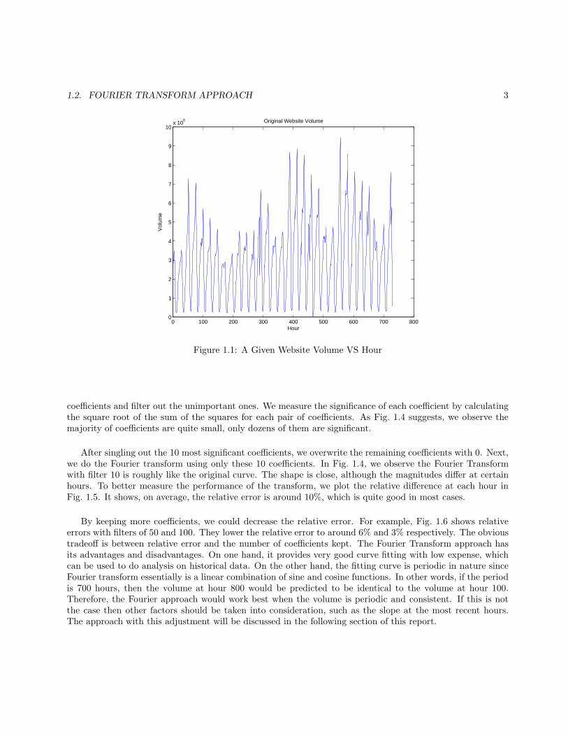
1.2 Fourier Transform Approach
Fig. 1.1 shows the original data of one particular website, that is referred to as niche67.The horizontal axis represents hours; hour 1 corresponds to the starting point of the data, 12:00 am on
6/24/2006, and the ending hour 729 represents the last recorded data point, 8:00 am on 7/24/2006. Thevertical axis is a particular website’s volume. We thought the first step to predict future volume would be tofind a pattern in historical data. Subsequently, we would try to find a function whose graph fits the historicaldata well.
From Fig. 1.1, we can observe a periodic pattern in the volume. Specifically, the website’s volume is quiteconsistent from one week to the next. Based on this observation, we thought it might be prudent to do aFourier transform on the historical data. Initially, we used a built-in Curve Fitting Tool(CFTOOL) interfacein Matlab to fit the data with Fourier transform. However, the maximum degree CFTOOL can offer forFourier fitting is 8 a nd our 1-month data contains 700+ hours. The 8-degree Fourier transform does not fitour data very well, which can be seen from Fig. 1.2.
To obtain a better fitting, we wrote a Matlab script which can use at most 728 degrees. When usingthis maximum, we observe that the Fourier transform is quite successful, as seen in Fig. 4.3. The absoluteerror between the data and fit is also plotted in Fig. 4.3 and is consistently on the scale of 10−9. However,the problem with this high degree transform is that there are more than 700 coefficients involved, which isobviously neither efficient nor convenient to deal with. As a result, we try to single out the most significant
1.2. FOURIER TRANSFORM APPROACH 3
0 100 200 300 400 500 600 700 8000
1
2
3
4
5
6
7
8
9
10x 10
6
Hour
Vol
ume
Original Website Volume
Figure 1.1: A Given Website Volume VS Hour
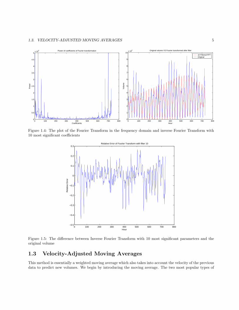
coefficients and filter out the unimportant ones. We measure the significance of each coefficient by calculatingthe square root of the sum of the squares for each pair of coefficients. As Fig. 1.4 suggests, we observe themajority of coefficients are quite small, only dozens of them are significant.
After singling out the 10 most significant coefficients, we overwrite the remaining coefficients with 0. Next,we do the Fourier transform using only these 10 coefficients. In Fig. 1.4, we observe the Fourier Transformwith filter 10 is roughly like the original curve. The shape is close, although the magnitudes differ at certainhours. To better measure the performance of the transform, we plot the relative difference at each hour inFig. 1.5. It shows, on average, the relative error is around 10%, which is quite good in most cases.
By keeping more coefficients, we could decrease the relative error. For example, Fig. 1.6 shows relativeerrors with filters of 50 and 100. They lower the relative error to around 6% and 3% respectively. The obvioustradeoff is between relative error and the number of coefficients kept. The Fourier Transform approach hasits advantages and disadvantages. On one hand, it provides very good curve fitting with low expense, whichcan be used to do analysis on historical data. On the other hand, the fitting curve is periodic in nature sinceFourier transform essentially is a linear combination of sine and cosine functions. In other words, if the periodis 700 hours, then the volume at hour 800 would be predicted to be identical to the volume at hour 100.Therefore, the Fourier approach would work best when the volume is periodic and consistent. If this is notthe case then other factors should be taken into consideration, such as the slope at the most recent hours.The approach with this adjustment will be discussed in the following section of this report.

4 CHAPTER 1. WEBSITE VOLUME PREDICTION
0 100 200 300 400 500 600 700
0
1
2
3
4
5
6
7
8
9
x 106
Vol vs. HourIndexfit 1
Figure 1.2: The filtered data using 8 selected coefficients, the solid line represents the fitting curve, and dotsdenotes the original data
0 100 200 300 400 500 600 700 8000
1
2
3
4
5
6
7
8
9
10x 10
6
Hour
Vol
ume
Fourier Transform on Volume
0 100 200 300 400 500 600 700 800−3
−2.5
−2
−1.5
−1
−0.5
0
0.5
1
1.5
2x 10
−9
Hour
Abs
olut
e E
rror
Absolute error between Fourier transformed and original volume
Figure 1.3: Left figure shows Fourier Transform on volume with 728 selected coefficients and right figure showsdifferences between Fourier transform and original volume
1.3. VELOCITY-ADJUSTED MOVING AVERAGES 5
0 100 200 300 400 500 600 700 8000
0.5
1
1.5
2
2.5
3
3.5
4
4.5
5x 10
8
Coefficients
Pow
er
Power of coefficients of Fourier transformation
0 100 200 300 400 500 600 700 8000
1
2
3
4
5
6
7
8
9
10x 10
6
HourV
olum
e
Original volume VS Fourier transformed after filter
10 Filtered FFTOriginal
Figure 1.4: The plot of the Fourier Transform in the frequency domain and inverse Fourier Transform with10 most significant coefficients
0 100 200 300 400 500 600 700 800−0.5
−0.4
−0.3
−0.2
−0.1
0
0.1
0.2
0.3Relative Error of Fourier Transform with filter 10
Hour
Rel
ativ
e E
rror
Figure 1.5: The difference between Inverse Fourier Transform with 10 most significant parameters and theoriginal volume
1.3 Velocity-Adjusted Moving Averages
This method is essentially a weighted moving average which also takes into account the velocity of the previousdata to predict new volumes. We begin by introducing the moving average. The two most popular types of

6 CHAPTER 1. WEBSITE VOLUME PREDICTION
0 100 200 300 400 500 600 700 800−0.3
−0.25
−0.2
−0.15
−0.1
−0.05
0
0.05
0.1
0.15
0.2Relative Error of Fourier Transform with filter 50
Hour
Rel
ativ
e E
rror
0 100 200 300 400 500 600 700 800−0.15
−0.1
−0.05
0
0.05
0.1
0.15
0.2
0.25Relative Error of Fourier Transform with filter 100
HourR
elat
ive
Err
or
Figure 1.6: The difference between Inverse Fourier Transform with 50 (100) most significant parameters andthe original volume
the moving average method are the Simple Moving Average (SMA) and the Exponential Moving Average(EMA). A simple moving average is formed by computing the average (mean) volume of a website over aspecified number of periods. All moving averages are lagged indicators. To reduce the lag in simple movingaverages, one often uses exponential moving averages (also called exponentially weighted moving averages).EMA reduces the lag by applying more weight to recent volumes relative to older volumes. The calculationassociated with the EMA is much more expensive than the calculation using a SMA.
To predict the volume at a specified time, we average over multiple days the corresponding hour’s volume,that is
A(t) =
n∑
i=1
WiXi(t) (1.1)
where n is the total number of days we are using, Xi(t) is the niche’s volume of the ith day at the tth hour,and the Wi are the related weights via the exponentially weighted moving average algorithm (EWMA),
Wi = (1 − λ)λn−i. (1.2)
The weights decrease exponentially as we move further back in the past, so that more emphasis is put on recentdata. We then take the data from previous days and find the slope of the smoothing spline approximatingthe past data points to approximate the shift in velocities, which are called Vi(t). Taking the same weights asabove, we get the average slope by
S(t) =n∑
i=1
WiVi(t). (1.3)
This is used to obtain the velocity by evolving the previous volume along the slope,
V EL(t) = Xn(t− 1) + S(t). (1.4)

1.4. POLYNOMIAL FITTING METHOD 7
We repeat using the previous volume along with the current average slope to generate a prediction for thenext time period.
1.3.1 Methodology
The procedure runs as follows. We begin with a set of past data along with a weight and specified lag between1 and 4(though this is not capped). The process assumes that the delayed reception of data takes place slightlybefore the new prediction is made. We take the exponentially weighted moving average(EWMA) using theinputed constant.
Following this, we take the velocity average (VEL) described above and weight it using the same exponentialweight process. We take the mean of the two predictions for the first several iterations,
V (ti) =EWMA(ti) + V EL(ti)
2. (1.5)
After we begin receiving the delayed data, we slide the interval of past data forward to take the new informationinto account. Once we have this new data, we can evaluate how well our prediction fit the data at that time.Using this, we can weight our two predictions, EWMA(ti − j) and V EL(ti − j), using a lag of j hours. Wefind the appropriate β that solves
D(ti − j) = β(EWMA(ti − j)) + (1 − β)(V EL(ti − j)), (1.6)
where D(ti) is the actual data at time ti. If β ∈ [0, 1], we use this weight to make our latest prediction bytaking the weighted average of the two predictions. It can be seen that β > 1 implies that the weighted movingaverage is between the actual data and the velocity-based estimate and so we take only the weighted movingaverage in our new prediction. On the other hand, β < 0 implies that the velocity-based estimate is betweenthe data and the weighted moving average and so we take only this estimate for our prediction.
1.3.2 Remarks and Accuracy
After having run several sets of data through the process, we see that a combination of the two provides abetter estimate (Figs. 1.7-1.10).
A possible source for this improvement is that the velocity based prediction is able to adjust to a recentchange in volume magnitude. However, on its own it can be extremely erratic in terms of error, both relativeand absolute, as it can in a few time steps escape the actual data. This tends to be corrected by the weightedmoving average. We show the results from some simulated data. Each column of graphs corresponds to oneof the three prediction methods and the rows show actual volume, absolute error, and relative error:
R(ti) =|V (ti) −D(ti)|maxD(ti)
(1.7)
where V (ti) is the prediction given by the above process. The model does suffer a performance drop underlonger lag periods, but does perform better than the EWMA method on its own. The model tends to performworse when less data is available to make a prediction; however, this change is not great.
1.4 Polynomial Fitting Method
From Fig. 1.11 and Fig. 1.12, we can see that the volumes exhibit a weekly pattern. There are two peak values

8 CHAPTER 1. WEBSITE VOLUME PREDICTION
3.2042 3.2044 3.2046 3.2048
x 105
−5
0
5
10x 10
6 Velocities vs Data
Hour
Vol
ume
VelData
3.2042 3.2044 3.2046 3.2048
x 105
0
2
4
6
8x 10
6 EWMA vs Data
Hour
Vol
ume
3.2042 3.2043 3.2044 3.2045 3.2046 3.2047 3.2048
x 105
0
2
4
6
8x 10
6 Adjusted Average vs Data
Hour
Vol
ume
DataEWMA
DataAvg
3.2042 3.2043 3.2044 3.2045 3.2046 3.2047 3.2048
x 105
0
1
2
3
4x 10
6 Absolute Error of Velocity
Hour
Err
or
3.2042 3.2043 3.2044 3.2045 3.2046 3.2047 3.2048
x 105
0
1
2
3
4
5x 10
6 Absolute Error of EWMA
Hour
Err
or
3.2042 3.2043 3.2044 3.2045 3.2046 3.2047 3.2048
x 105
0
0.5
1
1.5
2
2.5x 10
6 Absolute Error of Average
Hour
Err
or
3.2042 3.2043 3.2044 3.2045 3.2046 3.2047 3.2048
x 105
0
0.1
0.2
0.3
0.4
0.5Relative Error of Velocity
Hour
Err
or
3.2042 3.2043 3.2044 3.2045 3.2046 3.2047 3.2048
x 105
0
0.2
0.4
0.6
0.8Relative Error of EWMA
Hour
Vol
ume
3.2042 3.2043 3.2044 3.2045 3.2046 3.2047 3.2048
x 105
0
0.1
0.2
0.3
0.4Relative Error of Average
Hour
Err
or
Figure 1.7: One month’s data used for predicting next day with one hour lag.
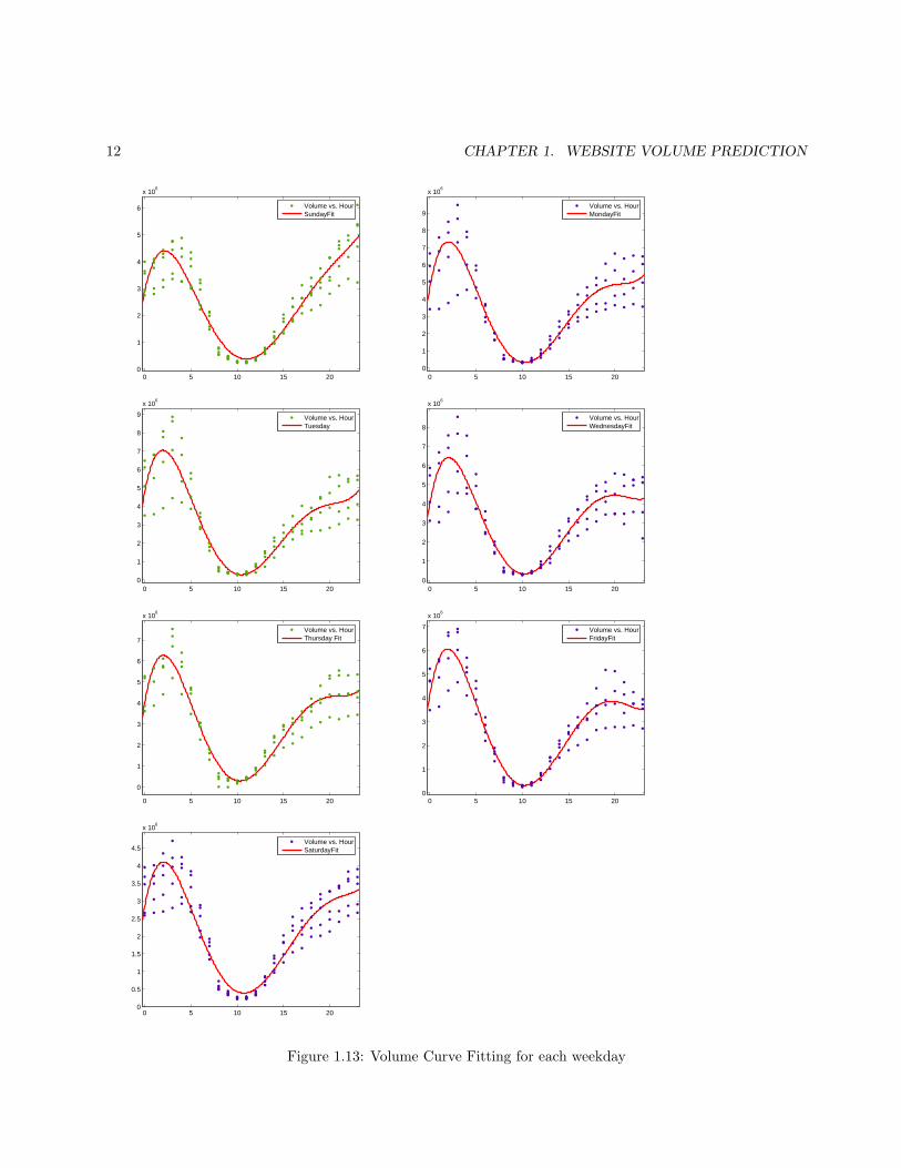
in each day: early morning and late night. At noon, volume reaches its lowest point of the day. For differentweekdays, we can see that peak values are quite different. But for the same weekday of different weeks, wecan see the peak values are similar.
Based on this observation, we model these weekdays separately. In Fig. 1.13, we can see 5th-order polyno-mial curve fitting for each weekday based on four weeks data. The common formula for 5th-order polynomialcurve fitting is as follows:
V = f(t) = p5t5 + p4t
4 + p3t3 + p2t
2 + p1t+ p0. (1.8)

1.4. POLYNOMIAL FITTING METHOD 9
3.2042 3.2044 3.2046 3.2048
x 105
−4
−2
0
2
4
6
8x 10
6 Velocities vs Data
Hour
Vol
ume
VelData
3.2042 3.2044 3.2046 3.2048
x 105
0
2
4
6
8x 10
6 EWMA vs Data
Hour
Vol
ume
3.2042 3.2044 3.2046 3.2048
x 105
0
2
4
6
8x 10
6 Adjusted Average vs Data
Hour
Vol
ume
DataEWMA
DataAvg
3.2042 3.2044 3.2046 3.2048
x 105
0
1
2
3
4
5
6x 10
6 Absolute Error of Velocity
Hour
Err
or
3.2042 3.2044 3.2046 3.2048
x 105
0
1
2
3
4
5x 10
6 Absolute Error of EWMA
Hour
Err
or
3.2042 3.2044 3.2046 3.2048
x 105
0
1
2
3
4
5x 10
6 Absolute Error of Average
Hour
Err
or
3.2042 3.2044 3.2046 3.2048
x 105
0
0.2
0.4
0.6
0.8Relative Error of Velocity
Hour
Err
or
3.2042 3.2044 3.2046 3.2048
x 105
0
0.2
0.4
0.6
0.8Relative Error of EWMA
Hour
Vol
ume
3.2042 3.2044 3.2046 3.2048
x 105
0
0.2
0.4
0.6
0.8Relative Error of Average
Hour
Err
or
Figure 1.8: Same month’s data used for predicting next day with four hours lag.

10 CHAPTER 1. WEBSITE VOLUME PREDICTION
3.1984 3.1985 3.1986 3.1987 3.1988
x 105
−2
0
2
4
6x 10
6 Velocities vs Data
Hour
Vol
ume
VelData
3.1984 3.1985 3.1986 3.1987 3.1988
x 105
0
2
4
6x 10
6 EWMA vs Data
Hour
Vol
ume
3.1984 3.1985 3.1986 3.1987 3.1988
x 105
0
2
4
6x 10
6 Adjusted Average vs Data
Hour
Vol
ume
DataEWMA
DataAvg
3.1984 3.1985 3.1986 3.1987 3.1988
x 105
0
0.5
1
1.5
2
2.5
3x 10
6 Absolute Error of Velocity
Hour
Err
or
3.1984 3.1985 3.1986 3.1987 3.1988
x 105
0
0.5
1
1.5
2
2.5
3x 10
6 Absolute Error of EWMA
Hour
Err
or
3.1984 3.1985 3.1986 3.1987 3.1988
x 105
0
0.5
1
1.5
2x 10
6 Absolute Error of Average
Hour
Err
or3.1984 3.1985 3.1986 3.1987 3.1988
x 105
0
0.1
0.2
0.3
0.4Relative Error of Velocity
Hour
Err
or
3.1984 3.1985 3.1986 3.1987 3.1988
x 105
0
0.2
0.4
0.6
0.8Relative Error of EWMA
Hour
Vol
ume
3.1984 3.1985 3.1986 3.1987 3.1988
x 105
0
0.1
0.2
0.3
0.4Relative Error of Average
HourE
rror
Figure 1.9: Four days data used for predicting next day with one hour lag.
3.1984 3.1985 3.1986 3.1987 3.1988
x 105
−2
0
2
4
6x 10
6 Velocities vs Data
Hour
Vol
ume
VelData
3.1984 3.1985 3.1986 3.1987 3.1988
x 105
0
2
4
6x 10
6 EWMA vs Data
Hour
Vol
ume
3.1984 3.1985 3.1986 3.1987 3.1988
x 105
0
2
4
6x 10
6 Adjusted Average vs Data
Hour
Vol
ume
DataEWMA
DataAvg
3.1984 3.1985 3.1986 3.1987 3.1988
x 105
0
1
2
3
4x 10
6 Absolute Error of Velocity
Hour
Err
or
3.1984 3.1985 3.1986 3.1987 3.1988
x 105
0
1
2
3
4x 10
6 Absolute Error of EWMA
Hour
Err
or
3.1984 3.1985 3.1986 3.1987 3.1988
x 105
0
1
2
3
4x 10
6 Absolute Error of Average
Hour
Err
or
3.1984 3.1985 3.1986 3.1987 3.1988
x 105
0
0.2
0.4
0.6
0.8Relative Error of Velocity
Hour
Err
or
3.1984 3.1985 3.1986 3.1987 3.1988
x 105
0
0.2
0.4
0.6
0.8Relative Error of EWMA
Hour
Vol
ume
3.1984 3.1985 3.1986 3.1987 3.1988
x 105
0
0.2
0.4
0.6
0.8Relative Error of Average
Hour
Err
or
Figure 1.10: Four days data used for predicting next day with four hours lag.

1.4. POLYNOMIAL FITTING METHOD 11
0 5 10 15 20 25 300
2
4
6
8
10x 10
6
Vol
ume
Day
Figure 1.11: Volume changes in a month
0 50 100 150 2000
2
4
6
8
10x 10
6
Hour
Vol
ume
First WeekSecond WeekThird WeekFourth week
Figure 1.12: Volume changes in a week
12 CHAPTER 1. WEBSITE VOLUME PREDICTION
0 5 10 15 200
1
2
3
4
5
6
x 106
Volume vs. HourSundayFit
0 5 10 15 200
1
2
3
4
5
6
7
8
9
x 106
Volume vs. HourMondayFit
0 5 10 15 200
1
2
3
4
5
6
7
8
9
x 106
Volume vs. HourTuesday
0 5 10 15 200
1
2
3
4
5
6
7
8
x 106
Volume vs. HourWednesdayFit
0 5 10 15 20
0
1
2
3
4
5
6
7
x 106
Volume vs. HourThursday Fit
0 5 10 15 200
1
2
3
4
5
6
7
x 106
Volume vs. HourFridayFit
0 5 10 15 200
0.5
1
1.5
2
2.5
3
3.5
4
4.5
x 106
Volume vs. HourSaturdayFit
Figure 1.13: Volume Curve Fitting for each weekday

1.4. POLYNOMIAL FITTING METHOD 13
Day P5 P4 P3 P2 P1 P0Sunday 26.27 -1903 4.937e+004 -5.139e+005 1.6e+006 2.888e+006Monday 68.45 -4605 1.098e+005 -1.054e+006 3.048e+006 4.646e+006Tuesday 61.35 -4120 9.833e+004 -9.451e+005 2.682e+006 4.74e+006Wednesday 57.29 -3930 9.51e+004 -9.224e+005 2.707e+006 3.978e+006Thursday 56.07 -3817 9.193e+004 -8.892e+005 2.587e+006 3.982e+006Friday 51.55 -3529 8.496e+004 -8.157e+005 2.296e+006 4.102e+006Saturday 27.07 -1920 4.823e+004 -4.843e+005 1.429e+006 2.829e+006
Table 1.1: The coefficients for the polynomial fit in Fig. 1.13
Day SSE R-square Adjusted R-square RMSESunday 3.539e+013 0.8792 0.8739 5.572e+005Monday 9.973e+013 0.8115 0.801 1.053e+006Tuesday 8.127e+013 0.8282 0.8187 9.503e+005Wednesday 8.419e+013 0.7918 0.7803 9.672e+005Thursday 4.36e+013 0.879 0.8723 6.96e+005Friday 3.525e+013 0.8863 0.88 6.259e+005Saturday 2.589e+013 0.8655 0.8596 4.766e+005
Table 1.2: Measures of fit for the polynomial curve fitting seen in Fig. 1.13.
We used a 5th-order polynomial to fit the data in each weekday, which resulted in 7 polynomial functions.Their parameters are listed in Table 1.1 and the goodness of fit is shown in Table 1.2. We use f(t, i), i ∈0, 1, ..., 6 to denote the curve we use to base our prediction on data from the ith day of week (Sunday is the0th day and Saturday is the 6th day). For instance, f(t, 0) represents the curve we get based on data fromSundays.
So the predicted volume can be obtained by
V = f(t, i) = p5(i)t5 + p4(i)t
4 + p3(i)t3 + p2(i)t
2 + p1(i)t+ p0(i). i ∈ 0, 1, ..., 6, t ∈ 0, 1, ..., 23. (1.9)
pj(i) represents the parameter pj on the ith day of the week. However, the theory value usually does not fitthe actual volume very well and we need to adjust our prediction based on the difference between actual valueand predicted value. There are several methods available to do that, however, we have focused on the movingaverage method. For our method, we assume that the curve for each weekday will stay almost the same.However, we will also take the difference between actual value and predicted value into account. So we willapply the weight vector to the theory value and previous volumes. For example, suppose we use the previoustwo weeks’ data to predict the volume with weight vector [0.1, 0.3, 0.6]. On the same day in the previous twoweeks, volumes are V ol((t−7)∗ 24) and V ol((t−2)∗ 7 ∗ 24)(t is the current hour, i denotes on which day t is),respectively. Then the predicted volume is PreV (t) = 0.6f(t mod 24, i) + 0.3V ol((t − 7) ∗ 24) + 0.1V ol((t −2) ∗ 7 ∗ 24).

14 CHAPTER 1. WEBSITE VOLUME PREDICTION
1.4.1 Our Strategy for Special Scenarios
The algorithm we discussed above does not account for some special cases of website volume behavior. Inorder to address these situations, we have added automatic adaption into our algorithm.
1. Periodical Shutdown
If the period for the shutdown is exactly one week, our algorithm can work without adjustment. However,if the period is not one week, our assumption that the volume will follow DOW is no longer true. We usuallycannot pinpoint the time when a server is shut down. We can get the period T of shutdown according to thepoints where volume is zero. Assuming we want to predict ith-hour’s volume, we will apply the weight vectorto i − T , i − 2T , i − 3T . This way, we can make the prediction match the actual volume accurately. Thefollowing function can give us the prediction,
PreV (t) = V ol(t− T ) ∗W (1) + V ol(t− 2T ) ∗W (2) + V ol(t− 3T ) ∗W (3), (1.10)
where PV (i) is the predicted volume for hour t, V (t) is real volume in hour t and W (i) is the weightvector’s ith element.
0 100 200 300 400 500 600 700−0.5
0
0.5
1
1.5
2
2.5
3
3.5x 10
4
Hour
Vol
ume
actual volumepredicted volumedifference
Figure 1.14: Prediction for periodic shutdown (based on two weeks data we predict the coming two week’svolume)
From Fig. 1.14, we can see that our strategy works well in this scenario.
2. Random Shutdown
For random shutdown, we did not find a very effective method. However, we assume that a website’svolume pattern will remain similar. So if we want to predict a website’s volume after a shutdown S, we willtrace back to find the latest shutdown S1 and use S1’s volume as the prediction. We did not realize this in

1.4. POLYNOMIAL FITTING METHOD 15
our algorithm. On the other hand, when we get some data indicating the volume for a website is quite low,the program will generate a warning.
3. State Change
When a website’s volume pattern changes suddenly, our algorithm will fail to predict a reasonable volumefor a website. We assume that the shape will stay the same although the magnitude will change. So we willchange the parameters of the seven curves for each weekday accordingly.
Now we determine a scale factor according to the ratio r of average volume in the past one day to theaverage volume in the past one week. If r > 1.6 or r < 0.6, we will multiply pi(i ∈ 0, 1, ..., 5) by r. We canexpress the function as follows:
r =
1
24
24−1∑
i=0
(PreV (t− l − i) − V ol(t− l− i))
1
168
7∗24−1∑
i=0
(PreV (t− l − i) − V ol(t− l − i))
(1.11)
V ol(i) is the real volume in the ith hour. PreV (i) is the predicted volume for the ith hour. l is the time lag.Fig. 1.15 shows an example of a prediction when volume increases dramatically. We can see that the
prediction follows the actual volume curve.
0 100 200 300 400 500 600 700−4
−2
0
2
4
6
8
10x 10
6
Hour
Vol
ume
actual volumepredicted volumedifference
Figure 1.15: Prediction for state change, volume increases significantly(based on two weeks data we predictthe coming two weeks volume)
Fig. 1.16 shows an example of prediction when volume decreases dramatically.

16 CHAPTER 1. WEBSITE VOLUME PREDICTION
0 200 400 600 800−4
−2
0
2
4
6
8x 10
6
Hour
Vol
ume
actual volumepredicted volumedifference
Figure 1.16: Prediction for state change, volume decreases significantly (based on two weeks data we predictthe coming two weeks volume)
4. Slight State Change
If the data we use is slightly different from the incoming data, we adjust our prediction according to thefollowing three measures:
First, if the hour to be predicted (we use t to represent it) is within rush hours (i.e. 19-6 GMT, thoughwe can adjust the definition according to specific time zones), we will adjust the prediction according to theprediction error in the latest three hours, i.e. from t− l− 2 to t− l (l is the data lag) if these three hours arein the rush hours. Before denoting the adjustment, we define function IsRushHour(t) first,
IsRushHour(t) =
1, if t is between 19pm and 6am0, otherwise
(1.12)
ErrorPercent1 =
2∑
j=0
(PreV (t− l − j) − V ol(t− l − j))
maxVIsRushHour(t− l − j)
∑2h=0 IsRushHour(t− l − h)
(1.13)
Adjust1 =
−MaxV ∗ ErrorPercent, if ErrorPercent1′s absolute value is bigger than 0.050, otherwise
(1.14)
where
maxV = Max(V ol(t− l − i)), 0 ≤ i ≤ 7 ∗ 24 (1.15)

1.4. POLYNOMIAL FITTING METHOD 17
Second, if the hour to be predicted is within rush hours(i.e. 19-6 GMT), we will adjust the predictionaccording to prediction error in the past t− 25 to t− 23 hours if these hours are in the rush hours.
ErrorPercent2 =
1∑
j=−1
(PreV (t− 24 − j) − V ol(t− 24 − j))
maxVIsRushHour(t− 24 − j)
∑1h=−1 IsRushHour(t− 24 − h)
(1.16)
Adjust2 =
−MaxV ∗ ErrorPercent, if ErrorPercent2′s absolute value is bigger than 0.050, otherwise
(1.17)
Third, we will adjust the prediction according to the average error in the past day if the average error isbigger than some threshold.
Adjust3 = −
23∑
j=0
(PreV (t− 24 − j) − V ol(t− 24 − j))
24(1.18)
Then we will add a weighted average of three adjustments to the prediction.
Adjust = W1 ∗Max(Adjust1, Adjust2) +W2 ∗Adjust3. (1.19)
Fig. 1.17 shows an example.
0 100 200 300 400 500 600 700−4
−2
0
2
4
6
8
10x 10
6
Hour
Vol
ume
actual volumepredicted volumedifference
Figure 1.17: Prediction for state slight change (based on two weeks data we predict the coming two weeksvolume)

18 CHAPTER 1. WEBSITE VOLUME PREDICTION
5. Special Days
For special days such as Mother’s Day, Independence Day etc., we need data on these days to predictwhether they follow some pattern. If they follow the same pattern, we can use previous special days to predictthe coming special day. If not, we check whether some special day has similar features. For instance, we checkall Mother’s Days in the past.
1.4.2 Simulation Result
In Fig. 1.18, we can see an example of our prediction using our method with weight vector [0.05, 0.2, 0.8, 0.05].Based on data in the past three weeks and the volume we calculated from the fitting curves, we take weightedaverage and get our prediction. We can see that our prediction follows the actual curve well. However, thedifference is large when there is a dramatic change.
0 100 200 300 400 500 600 700 800−2
0
2
4
6
8
10x 10
6
Hour
Vol
ume
actual volumepredicted volumedifference
Figure 1.18: Prediction based former three weeks’ data for the coming one week
In Fig. 1.19, we show the average errors of moving averages under different weight averages. The vector[0.5, 0.5, 0] corresponds to the simple moving average method. It takes the average volume of the past twoweeks on the same day as the prediction value and involves no curve fitting. We can see that when the weightfor the theory value obtained from Eqn. 1.9 increases, the average error decreases except when its weight is0.1. When the weight for the most recent data is large, average error is even worse than the SMA. However,we cannot say that when the weight for the theory value is large, WMA will perform better than it will whenthe weight for the theory value is small. We need other standards to evaluate this method.
1.5 Comparison
If we compare these three approaches, we see each has its advantages and disadvantages.

1.5. COMPARISON 19
0 2 4 6 8 10 12 14 16 180
0.5
1
1.5
2
2.5
3x 10
6
website
aver
age
erro
r
[0.5 0.5 0][0.2 0.4 0.4][0.1 0.6 0.3][0.1 0.3 0.6][0.1 0.8 0.1][0.1 0.1 0.8]
Figure 1.19: Average Error of moving average method with different weight vector for 18 websites
The Fourier transform approach requires the largest amount of data to observe a possibly periodic patternand the corresponding length of each period. Therefore, if we have several months’ or years’ data, and we wantto have a long-term picture about website volume, then we can try the Fourier transform to fit the historicaldata and predict the future based on the filtered Fourier function. However, the Fourier transform approachis not good at predicting short-term volume since it is not sensitive to the most recent trend.
To predict website volume in the coming hours, Velocity-Adjusted Moving Average approach would be thebest choice. This approach only requires historical data from the past couple of days, instead of data frompast years as required by the Fourier transform approach. However it becomes more accurate with more data,reaching reasonable errors with 2-4 weeks of data. Another advantage is that it catches the current trendvery well. It takes the slope, i.e. the velocity of volume into consideration, and predicts future volume basedon the weighted average of Exponentially Weighted Moving Average and Velocity Average. In particular, theweight is dynamically decided based on the most recent incoming data. This approach is more accurate whenpredicting short period and becomes less reliable when the prediction period becomes longer, because the errorfrom each step accumulates and could become quite large after a couple of weeks.
The Polynomial Fitting lies somewhere in the middle between Fourier Approach and Velocity-AdjustedMoving Average approach. It requires several weeks’ instead of years’ or days’ historical data to do theprediction. Contrast to Velocity-Adjusted Moving Average approach, it is capable of predicting longer period.With two weeks’ historical data, we have predicted the following two weeks’ volume with satisfactory relativeerrors. Another nice feature is that this approach includes a prediction tube, or range, which is used todetects slight state change and drastic state change. Then it handles them separately. For slight state change,it makes prediction adjustments based on recent prediction errors. For a large state change, it calculatesthe multiplier and imposes it on the original polynomial. The major drawback of this approach is that itcan not effectively deal with sudden drastic pattern changes, which includes not only magnitude changes butalso shape changes. Fortunately, this situation doesn’t happen very often in most websites. When this does

20 CHAPTER 1. WEBSITE VOLUME PREDICTION
happen, the Velocity-Adjusted Moving Average can be applied to make short-term prediction.Based on business needs and historical data, and how long we want to predict into the future, we can make
the best choice among these three approaches.
1.6 Conclusion and Future Work
For the second and third model, we simply fixed some parameters and so these parameters are likely notoptimal. Probably we should study the relationship between the optimal value and different configurationsand develop some strategy to adjust our parameters to achieve the best performance. Moreover, we shouldrun our program with large real historical data to see their average performance. Finally, we should realizethe Kalman Filter method and compare its performance with ours.

Bibliography
[1] “Moving average”, http://www.stockcharts.com/education/IndicatorAnalysis/indic movingAvg.html.
[2] “Time Series Analysis”, http://www.statsoft.com/textbook/sttimser.html.
[3] “Introduction to Time Series Analysis”, http://www.itl.nist.gov/div898/handbook/pmc/section4/.
[4] “The R Project for Statistical Computing”, http://www.r-project.org/.
[5] Quarteroni, A., Sacco, R. and Saleri, F. (2000) Numerical Mathematics, Springer.
[6] Popova, E. and Wilson, J.G. (2000) Adaptive time dynamic model for production volume prediction,INT.J.Prod, 38(13):3111-3130.
[7] Bellanger, M. (1984) Digital Processing Of Signals, Theory And Practice, John Wiley and Sons, UK.
[8] Stein, J. (2000) Digital Signal Processing, A Computer Science Perspective, John Wiley and Sons, USA.
[9] Jiang, R. and Szeto, K.Y (2003) Extraction of investment strategies based on moving averages: A geneticalgorithm approach, Computational Intelligence for Financial Engineering, pp. 403-410.
[10] Tabbane, N., Tabbane, S. and Mehaoua, A. (2004) Autoregressive, moving average and mixedautoregressive-moving average processes for forecasting QoS in ad hoc networks for real-time servicesupport, Vehicular Technology Conference(VTC), 5:2580-2584.
[11] Dandawate, A. and Giannakis, G.B (1996) Modeling (almost) periodic moving average processes usingcyclic statistics, IEEE Transactions on Signal Processing, 44(3):673-684.
21

22 BIBLIOGRAPHY

Chapter 2
Optimal Implied Views for Skewed
Return Distributions
Robertas Gabrys1, Weihua Geng2, Rachel Koskodan3, Jing Li4, Luke Owens 5, Qi Wu 6,Miao Zuo7
Problem Presenter:Randy Miller
Bank of America
Faculty Consultants:Dr. Tao Pang and Dr. Jeff ScroggsNorth Carolina State University
Abstract
An important aspect of banking is determining how optimally to allocate a fixed quantity of money amongdifferent companies requesting loans from a bank. This problem can be mathematically formulated as a mini-mization (of risk) or a maximization (of utility) problem with certain constraints. We solve this minimizationproblem using two different measures of risk and varying constraints. We also solve the maximization prob-lem for certain utility functions. In addition to this optimal allocation problem, banks face the challenge of
1Utah State University2Michigan State University3Texas Tech University4UNC-Charlotte5University of South Carolina6University of South Carolina7Arizona State University
23
24 CHAPTER 2. OPTIMAL IMPLIED VIEWS FOR SKEWED RETURN DISTRIBUTIONS
communication among different portfolio managers, as each has his/her own view on the correct allocationof the assets. A possible approach to this problem is determining the necessary implied returns of each man-ager’s portfolio position. This would indicate how far his/her portfolio allocation is from the mathematicallydetermined optimal allocation. The challenge of determining the implied returns is the inverse of the aboveproblem. We solve this problem using the same measures of risk and utility.
2.1 Introduction
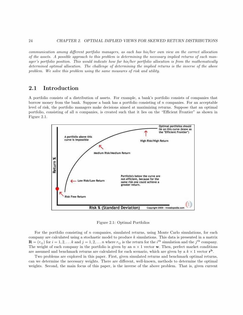
A portfolio consists of a distribution of assets. For example, a bank’s portfolio consists of companies thatborrow money from the bank. Suppose a bank has a portfolio consisting of n companies. For an acceptablelevel of risk, the portfolio managers make decisions aimed at maximizing returns. Suppose that an optimalportfolio, consisting of all n companies, is created such that it lies on the “Efficient Frontier” as shown inFigure 2.1.
Figure 2.1: Optimal Portfolios
For the portfolio consisting of n companies, simulated returns, using Monte Carlo simulations, for eachcompany are calculated using a stochastic model to produce k simulations. This data is presented in a matrixR = (rij) for i = 1, 2, . . . k and j = 1, 2, . . . n where rij is the return for the ith simulation and the jth company.The weight of each company in the portfolio is given by an n × 1 vector w. Then, perfect market conditionsare assumed and benchmark returns are calculated for each scenario, which are given by a k × 1 vector rb.
Two problems are explored in this paper. First, given simulated returns and benchmark optimal returns,can we determine the necessary weights. There are different, well-known, methods to determine the optimalweights. Second, the main focus of this paper, is the inverse of the above problem. That is, given current
2.2. MINIMUM CV AR METHOD 25
−5 0 50
0.05
0.1
0.15
0.2
0.25
0.3
0.35
0.4Normal distribution
VaR
CVaR
Figure 2.2: VaR and CVaR in Standard Normal Distribution
weights and benchmark returns, can we derive the implied expected returns that make the portfolio optimal.Three approaches to solve the above problems are considered. Section 2.2 examines solutions that minimizethe conditional-value-at-risk, CV aR. Section 2.3 examines solutions that minimize the tracking error in amean-square sense. Section 2.4 examines solutions found using an extended Black-Litterman (EBL) approach.
To compare the three approaches, an example using a 10 company portfolio is examined for solving theinverse problem using each of the three methods described in Sections 2.2-2.4. The model problem considersthe returns of the first 400 simulations of the first 10 companies with the corresponding benchmark returnvector, and assumes that the assets are distributed equally among all 10 companies. That is, w(i) = 0.1 for1 ≤ i ≤ 10.
2.2 Minimum CV aR method
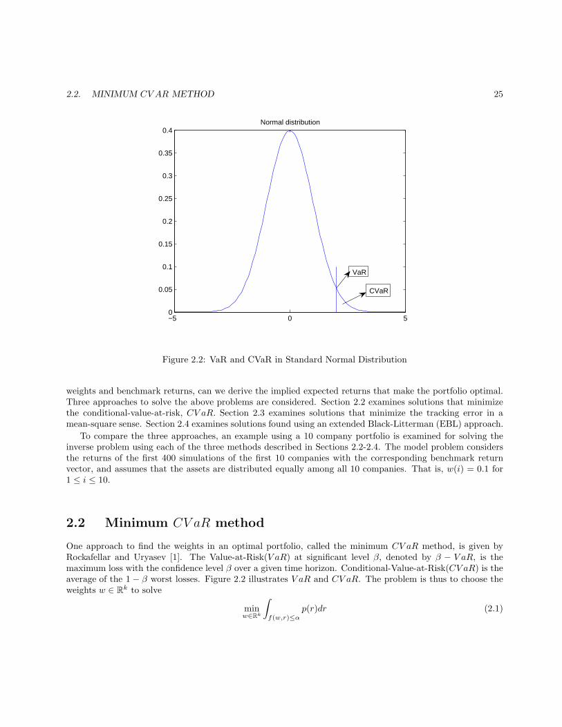
One approach to find the weights in an optimal portfolio, called the minimum CV aR method, is given byRockafellar and Uryasev [1]. The Value-at-Risk(V aR) at significant level β, denoted by β − V aR, is themaximum loss with the confidence level β over a given time horizon. Conditional-Value-at-Risk(CV aR) is theaverage of the 1 − β worst losses. Figure 2.2 illustrates V aR and CV aR. The problem is thus to choose theweights w ∈ Rk to solve
minw∈Rk
∫
f(w,r)≤α
p(r)dr (2.1)

26 CHAPTER 2. OPTIMAL IMPLIED VIEWS FOR SKEWED RETURN DISTRIBUTIONS
where f(w, r) is the loss function whose detailed definition will be given later, α is β − V aR, p(r) is theprobability distribution function, pdf, of the random variable r. Rockafellar and Uryasev showed the aboveproblem is equivalent to a linear programming problem on a convex set. The MatLab optimization toolboxcan solve this problem directly using the command linprog.
On the other hand, the inverse problems of this optimization problem will be considered. One thing welike to point out is that, if we solve for returns given the weights, there will be many more unknowns thanequations. Therefore, it will be an under-determined problem if we following that direction. There is anotherpossible way. First we compute variance and covariance implied by historic data. Then, we use the variance,covariance information and the return at each mode to simulate a new return of each company and then geta new w∗. In this way, at each mode of discretized return space, we have an optimal weight corresponding toit. If there are some good properties of this correspondence (eg. monotonicity), then we can find the impliedreturn for a given set of weights. Unfortunately, this method cannot work either. First of all, if there are onlytwo or three companies, then there’s no problem of discretizing a two or three-dimension return space. Butif there are more than 5 (200 in our database) companies, then the discretization will become impractical.Secondly, there is no reason for the weight to be monotone with respect to the return in the large system ofhundreds of companies.
Therefore, instead of trying the straightforward methods we mentioned above, we tried the following twomethods to solve this problem:
1. Empirical Method : Solve for the weights given the returns and determine if there is a relationship betweenthem.
2. Parameterized Method : Analyze the relationship between the parameterized returns and the risk accord-ing to the given weights.
We have obtained some satisfactory results, and details will be given in the next two subsections.
2.2.1 Empirical Method
In this method, we are going to solve for weights, given the returns for each company. According to R-U [1],minimizing CV aR can be reduced to the linear programming problem:
minw∈Rn,z∈RJ ,α∈R
α+1
(1 − β)J
J∑
j=1
zj (2.2)
The constraints are
zj ≥ (bj −n∑
i=1
wirij) − α
zj ≥ 0
1 > wi > 0.001
1 =
n∑
i=1
wi

2.2. MINIMUM CV AR METHOD 27
Company V*M Var Mean Weight1 Weight2 Weight3 Weight4 Weight5
14 ~0 ~0 0.0001 0.976 throw away throw away throw away throw away
1 ~0 ~0 0.0002 0.001 0.977 throw away throw away throw away
15 ~0 ~0 0.0018 0.001 0.001 0.8981 throw away throw away
3 0.35 0.0005 0.0007 0.001 0.001 0.0809 0.979 throw away
19 0.42 0.0001 0.0042 0.001 0.001 0.001 0.001 0.3031
6 0.76 0.0002 0.0038 0.001 0.001 0.001 0.001 0.0978
17 1.02 0.0002 0.0051 0.001 0.001 0.001 0.001 0.2858
9 2.16 0.0009 0.0024 0.001 0.001 0.001 0.001 0.2964
13 2.78 0.0139 0.0002 0.001 0.001 0.001 0.001 0.001
8 3.4 0.001 0.0034 0.001 0.001 0.001 0.001 0.001
2 4.23 0.0009 0.0047 0.001 0.001 0.001 0.001 0.001
24 6.21 0.0069 0.0009 0.001 0.001 0.001 0.001 0.001
4 6.38 0.0011 0.0058 0.001 0.001 0.001 0.001 0.001
20 6.66 0.0018 0.0037 0.001 0.001 0.001 0.001 0.001
5 7.4 0.002 0.0037 0.001 0.001 0.001 0.001 0.001
25 7.56 0.0036 0.0021 0.001 0.001 0.001 0.001 0.001
12 9.75 0.0065 0.0015 0.001 0.001 0.001 0.001 0.001
23 10.83 0.0057 0.0019 0.001 0.001 0.001 0.001 0.001
7 15.39 0.0027 0.0057 0.001 0.001 0.001 0.001 0.001
10 23.56 0.0019 0.0124 0.001 0.001 0.001 0.001 0.001
22 23.76 0.0012 0.0198 0.001 0.001 0.001 0.001 0.001
11 24.75 0.0025 0.0099 0.001 0.001 0.001 0.001 0.001
18 30.45 0.0145 0.0021 0.001 0.001 0.001 0.001 0.001
21 34.8 0.006 0.0058 0.001 0.001 0.001 0.001 0.001
16 61.36 0.0104 0.0059 0.001 0.001 0.001 0.001 0.001
Figure 2.3: Relation of weight to mean and variance
where α is the V aR, b = (b1, ...bJ) is the benchmark, rij is historical return of ith company in the jth scenario,wi is the weight, zj ’s are dummy variables, i = 1, ..., n and j = 1, ...J .
There are two different ways to define the loss function. We will explore both of them next.
First Way to Define the Loss Function
The first definition of the loss function defines fj(w, r) =∑n
i=1(wirij). Figure 2.3 shows that companieswith very small average returns and very small variances will have the largest weights. To combine those twofactors, first we define mean return as µ and variance as σ2, then set up a trial function: g(µ, σ2) = µ× σ2.
As shown in Figure 2.3, for the first 400 scenarios of the 25 companies, companies 14, 1 and 15 have thesmallest trial function values. Company 14 has the minimum average return, the minimum variance, and hasthe largest weight, 0.976. If we discard the company with the minimum trial function value, and just considerthe remaining companies, then the company which has the second smallest trial function value will have thelargest weight, and so on. The covariances also have an impact on the weights. But in this investigationcovariances are not considered for the reason of complicity.
The conclusion is that the weight is approximately monotone with respect to the trial function g. Reviewingthe data, we see that the variance affects the value of weight. For instance, Company 14 has the smallestvariance, meaning it has stable returns and a very small risk of loss. Although the return is small, the companyis assigned a very large weight. Thus, for a given weight w = (w1, w2, . . . , w25), if a wi has a much largervalue than others, then the company corresponding to this weight should have a very small value of the trialfunction, compared to those companies that follow it in Figure 2.3.

28 CHAPTER 2. OPTIMAL IMPLIED VIEWS FOR SKEWED RETURN DISTRIBUTIONS
−5 0 5 10 15 20
x 10−3
0
0.2
0.4
0.6
0.8
mean
wei
ght
0 0.002 0.004 0.006 0.008 0.01 0.012 0.014 0.016 0.0180
0.2
0.4
0.6
0.8
variance
wei
ght
Figure 2.4: Relation of weight to mean and variance
Second Way to Define the Loss Function
In this part we consider the loss function defined as the following
fj(w, r) = bj −n∑
i=1
(wirij), (2.3)
where the bj is benchmark. Figure 2.4 shows the relation of weight versus the mean return along with theweight versus the variance of the return. There does not appear to be a clear relation between the weightand the mean. In the plot of the weight versus the variance, we can clearly see that the weight is high forcompanies with low variances. So a company with high risk tends to attain a small weight.
However, we believe that the means also play an important role in determining the weights. Intuitively,people invest in the assets with higher returns. We tried the trial function g(µ, σ) = µ − 2σ. This trialfunction makes perfect sense. For a normal distribution, the 5th percentile is approximately µ− 2σ, which isthe definition of V aR of the standardized normal distribution. For the normal distribution, minimizing V aRis equivalent to minimizing CV aR. We can see that the value of g is in the positive direction of the mean,and negative direction of the variance.
Figure 2.5 is the plot of weight versus the trial function g. It shows that there is some trend between theweight and the value of g. It is approximately a monotone increasing function. A reasonable conclusion isthat the higher the return of a company, the higher the weight of the company; the less the stability of thereturn of a company, the lower weight the company should have. Thus, for a given weight of a company, ifit is much higher than the other companies, it should be more stable and have a higher return as compared

2.2. MINIMUM CV AR METHOD 29
−0.3 −0.25 −0.2 −0.15 −0.1 −0.05 0 0.050
0.1
0.2
0.3
0.4
0.5
0.6
0.7
test function
we
igh
t
test function = mean - 2* SD
Figure 2.5: Relation between weight and trial function
with other companies.In the next subsection, how the weights affect the mean returns under the optimal assumption is analyzed.
2.2.2 Parameterized Method
In the previous section, we managed to see relationships between the weights and the returns. However, wecould not find one-to-one correspondence or an explicit function between them. Since this system is highlyunder-determined, we can change the assumption that the return of a certain company has the same changein different scenarios. The changes depend on the δ ∈ Rn. The vector of δ is called parameter. Thus theproblem becomes
minδ∈Rn,z∈RJ ,α∈R
α+1
(1 − β)J
J∑
j=1
zj (2.4)
s.t.
zj ≥ bj − (Rδw)j − α
zj ≥ 0
Here Rδ is the new return matrix with the ith column of this matrix defined as the corresponding column ofthe original matrix plus a constant δi. Since the magnitudes of mean of the each company are largely different,the numbers we add to each company are set to be proportional to the original mean of the company.

30 CHAPTER 2. OPTIMAL IMPLIED VIEWS FOR SKEWED RETURN DISTRIBUTIONS
0 0.005 0.01 0.015 0.02 0.025 0.03 0.035−0.02
0
0.02
0.04
0.0610000 scenarios
risk
retu
rn
0 0.005 0.01 0.015 0.02 0.025 0.03 0.035−0.02
0
0.02
0.04
0.06
0.08400 scenarios
risk
retu
rn
Figure 2.6: Relation between return and risk based on different number of scenarios
We did the numerical experiment for the first 10 companies. We are only able to use < 500 scenarios inproglin command in MatLab. 400 scenarios is too small to catch the basic rules in financial world. First, thelong run mean return should be nonnegative. In Figure 2.6, we can see for 10,000 scenarios there is only 1negative return, while there are several companies which have negative returns. Second, the empirical datashould have return increases when the risk increases. We can clearly see this pattern in the 10,000 scenarioplot. However in the 400 scenarios, even high risk companies have 0 returns.
In the following two methods, we are going to take the weight to be the same for all companies we chose.The empirical return increases with respect to the risk. Now if we set the weight to be the same, the newreturns corresponding to the given equal weights should also increase with respect to the risk.
Multiplicative Parameterize
A variation we consider is to multiply a constant to different company return. To minimize CV aR under thegiven weights, the magnitude of the return of each company in every scenario should increase by a multipleof the original return. Let δ = (δ1, ..., δn) be a vector of multiples, δi is the constant multiplied to ith column.Thus the problem is
minδ∈Rn,z∈RJ ,α∈R
α+1
(1 − β)J
J∑
j=1
zj (2.5)

2.2. MINIMUM CV AR METHOD 31
Company MultiplierOriginal Mean Variance New Mean New Variance Trial Function g
1 3.6845 0.0002 0.0021 0.0006 0.0078 -0.0062
2 2.3192 0.0052 0.0297 0.0121 0.069 -0.084
3 0.4319 0.0004 0.026 0.0002 0.0112 -0.0776
4 0.5573 0.0051 0.0371 0.0028 0.0207 -0.1063
5 0.4032 0.0051 0.0387 0.0021 0.0156 -0.111
6 2.4758 0.0034 0.0167 0.0084 0.0414 -0.0467
7 0.3084 0.0047 0.0578 0.0014 0.0178 -0.1687
8 0.2788 0.003 0.0343 0.0008 0.0096 -0.0999
9 0.4253 0.0022 0.032 0.0009 0.0136 -0.0937
10 0.9811 0.0115 0.048 0.0113 0.047 -0.1323
Figure 2.7: New return by given equal weight
s.t.
zj ≥ bj −n∑
i=1
wi(rijδi) − α
zj ≥ 0
Figure 2.7 shows the implied returns for each company. The implied returns are listed with the originalreturns, variances and the values of the trial function defined previously. We highlight four companies withhighest value of trial function. Out of those four companies, three get the highest multipliers. After plottingthe implied return against the historic variance, we can see some obvious relation between the return and therisk in Figure 2.8. The return increases with respect to the variance.
If we multiply a constant to a random variable, we are changing the mean and variance together. That isthe drawback of this method, since there is no reason that the mean and standard derivation should changetogether by the same amount. Moreover, if we change two quantities together, we are not able to see how theweight will impact each of them. We believe that is why we can not see the pattern in the mean or variancechange according to the given weight.
Additive Parameterize
Instead of multiplying a constant to each column, we want to improve the parameterized model by adding aconstant return to each company. Each column of this matrix is equal to the corresponding column of theoriginal matrix plus a constant. Considering the magnitude of the mean of each company is largely different,the numbers we add to each company are set to be proportional to the original mean of the company.
We consider the following problem:
minδ∈Rn,z∈RJ ,α∈R
α+1
(1 − β)J
J∑
j=1
zj (2.6)
32 CHAPTER 2. OPTIMAL IMPLIED VIEWS FOR SKEWED RETURN DISTRIBUTIONS
0 0.01 0.02 0.03 0.04 0.05 0.06 0.070
0.002
0.004
0.006
0.008
0.01
0.012
0.014
Risk (Variance)
Ret
urn
(Mea
n)
Equal Weight Under Multiplicative Model
Figure 2.8: Relation between risk and implied return
Company Variance Constant Mean return New mean
3 0.026 -0.4143 0.0004 0.0002
35 0.0333 -0.3566 0.0004 0.0003
171 0.0352 0.3175 0.0013 0.0017
28 0.038 1.2643 0.0041 0.0093
42 0.0388 -0.0834 0.0007 0.0007
54 0.0408 -0.0207 0.0008 0.0008
178 0.0417 -0.2228 0.0006 0.0004
132 0.0468 0.4848 0.0016 0.0023
138 0.0474 0.547 0.0017 0.0026
191 0.0477 0.6307 0.0019 0.0031
137 0.0565 1.243 0.004 0.0089
95 0.062 0.3569 0.0013 0.0018
100 0.0627 0.454 0.0015 0.0022
29 0.0742 1.4596 0.0054 0.0134
165 0.0743 1.3693 0.0047 0.0112
27 0.079 1.2952 0.0043 0.0098
140 0.0805 1.4437 0.0053 0.0129
21 0.0837 1.2368 0.0039 0.0088
133 0.0873 0.882 0.0026 0.0048
62 0.0911 1.5215 0.0061 0.0154
119 0.0942 1.5493 0.0098 0.025
189 0.0991 1.2338 0.013 0.0289
104 0.1153 1.4415 0.0112 0.0274
48 0.1455 1.086 0.0139 0.029
58 0.1636 0.0365 0.0208 0.0216
Figure 2.9: New return by given equal weight

2.2. MINIMUM CV AR METHOD 33
0.02 0.04 0.06 0.08 0.1 0.12 0.14 0.16 0.180
0.005
0.01
0.015
0.02
0.025
0.03
Risk (Variance)
Ret
urn
(Mea
n)
Equal Weight under Additive Model
Figure 2.10: Relation between risk and implied return
s.t. zj ≥ bj −n∑
i=1
wi(rij + δiri) − α
zj ≥ 0n∑
i=1
wiδi = 0
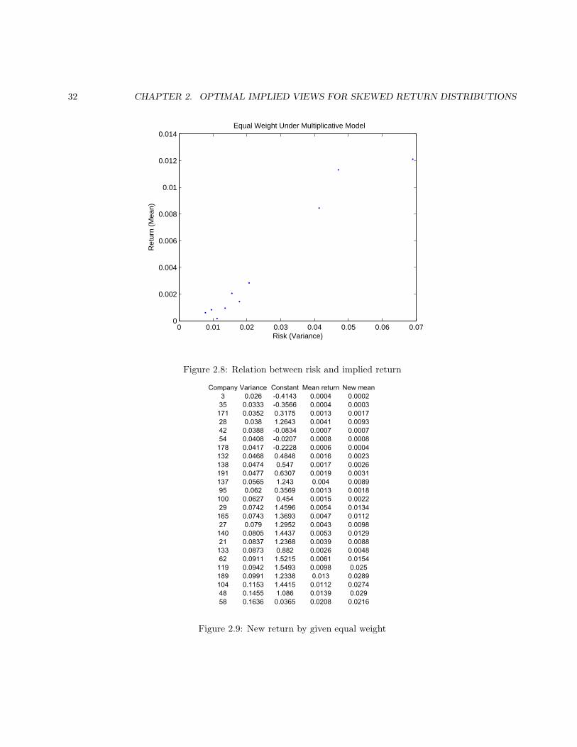
where ri is the mean of column i.Figure 2.9 shows the implied return for each company. Given equal weights, it is expected that the
companies with high risk have high returns. After plotting the implied return against the historic variance,we can see a positive trend between return and risk in Figure 2.10. So this kind of result is reasonable: Thecompany with a higher implied return generally has a higher risk of loss.
2.2.3 Conclusion
Thus, our conclusion of minimization of CV aR is
1. We are not able to find the one to one correspondence between the returns and the weights.
2. Some relationship can be found between the characteristics (mean, variance) of the return matrix andthe weights.
In the next section we will look at the method of minimizing the tracking error.

34 CHAPTER 2. OPTIMAL IMPLIED VIEWS FOR SKEWED RETURN DISTRIBUTIONS
2.3 Minimizing the Tracking Error
The tracking error(TE) is defined as
TE =
√√√√√k∑
i=1
n∑
j=1
rijwj − rbi
2
= ‖Rw− rb‖ , (2.7)
where ‖ · ‖ is the vector norm, R is the return matrix, w is the vector of weights, and rb is the benchmarkreturn. First, we wish to determine the weights of the companies that give expected portfolio returns closestto the optimal returns in a mean square sense. Then we will consider the inverse problem. That is, given areturn matrix, a vector of weights, and a benchmark vector, we try to determine how the return matrix hasto change to minimize TE.
First, we consider the problem of finding the vector of weights that minimizes TE when the return matrixand benchmark vector are given. This problem is analyzed with and without financially motivated constraintson the weights. Secondly, the inverse problem will be considered. We like to point out that the straightforwardinverse problem is not well-posed in the sense that given w and rb, there are infinitely many ways to changeR to minimize the tracking error. Hence, we put restrictions on how R is allowed to change in order to getmeaningful unique solutions.
2.3.1 Unconstrained Minimization
First, we investigate determining the weights that minimize the tracking error. That is, find w ∈ Rn such that
‖Rw− rb‖ (2.8)
is minimized.In general, we minimize ‖Ax− b‖2 over x ∈ Rn where A ∈ Rk×nand b ∈ Rk. Consider
‖Ax− b‖2 = (Ax − b)T (Ax − b)
= [(Ax)T − bT ][(Ax) − b]
= (Ax)T (Ax) − (Ax)Tb − bT (Ax) + bTb
= (Ax)T (Ax) − 2xTAT b + bT b.
The minimum is found by taking the derivative with respect to x and setting it equal to zero. By doing thatwe can get the normal equation
ATAx = ATb. (2.9)
If k ≥ n and A has full rank, then ATA can be inverted and the unique solution of the least squares problemis
x = (ATA)−1ATb
where (ATA)−1AT is called the pseudo-inverse of A.In financial situations it is nearly always the case that, k ≥ n, more simulations than companies, and A
is of full rank. There are a few well known methods for solving (2.9) with the above properties: Choleskydecomposition, QR-factorization, and singular value decomposition. The QR-factorization method is used

2.3. MINIMIZING THE TRACKING ERROR 35
with an outline as follows. Using a Gram-Schmidt orthonormalization process, factor A = QR, where Qis an orthogonal matrix (i.e QTQ = I), and R is an upper triangular matrix. Using equation (2.9), theorthogonality of Q, and the fact that R and RT are non-singular,
ATAx = AT b
=⇒ RT Rx = RTQTb
=⇒ Rx = QTb. (2.10)
Since R is an upper triangular matrix (2.10) is easily solved using back substitution. In Matlab the entireprocess is carried out with the command x = A \ b.
For the examples considered in this paper, R is a 10000×250 return matrix and rb is a 10000×1 benchmarkreturn vector. The data was provided by Bank of America.
First, we consider the unrestricted minimization problem. That is, the weights can assume any real numbervalue. The minimization problem (2.8) is solved using the Matlab command w∗ = R \ rb. Figure 2.11 is aplot of w∗.
50 100 150 200 250
0
0.02
0.04
0.06
0.08
0.1
0.12
0.14
0.16
0.18
Company
Pe
rce
nta
ge
of
Po
rtfo
lio
Weights for the Unconstrained Minimization Problem
Figure 2.11: Unconstrained Weights
This unconstrained w∗ yielded a mean square error of
TE = ‖Rw∗ − rb‖ = 0.2428 , (2.11)
and a plot of the point-wise scenarios error is given below in Figure 2.12.Figure 2.13 compares the optimally weighted portfolio returns to the benchmark returns. For illustration,
only every hundredth scenario is plotted.

36 CHAPTER 2. OPTIMAL IMPLIED VIEWS FOR SKEWED RETURN DISTRIBUTIONS
0 1000 2000 3000 4000 5000 6000 7000 8000 9000 100000
0.005
0.01
0.015
0.02
0.025
Scenarios
Erro
rAbsolute Error for Unconstrained Problem
Figure 2.12: Pointwise Error for the Unconstrained Problem
0 10 20 30 40 50 60 70 80 90 100−0.015
−0.01
−0.005
0
0.005
0.01
0.015
Scenarios
Retu
rn
Benchmark Returns and Optimal Weight Returns for 100 Scenarios
Optimal Weight ReturnsBenchmark Returns
Figure 2.13: Unconstrained Return Comparison
2.3. MINIMIZING THE TRACKING ERROR 37
As Figure 2.11 suggests, some of the components of w∗ are negative. In fact, 16 of the 250 weights arenegative. The financial interpretation of this is that the bank would not give a loan to these 16 companies, andwould short sell the companies bonds or stocks. However, it is often the case that the bank wants a portfolioconsisting only of long positions. So, the constrained problem will require the weights to be non-negative.
Another feature of the vector of weights w∗ is∑250
i=1 w(i) = 1.028. If we assume that there cannot be any
negative weights, so we set the negative components of w∗ equal to zero,∑250
i=1 w(i) = 1.0536. This says thatthe bank should invest 105.36% of the total amount they want to invest. This is obviously impossible. So,another constraint will require
∑250i=1 w(i) = 1 which exhausts the portfolio. Another approach is to set the
sum of the weights less than or equal to one and put the difference (1 −∑250i=1 wi) into a risk free investment.
2.3.2 Constrained Minimization
Non-negative weights and an exhausted portfolio are two constraints we just discussed. A third constraint isa minimum return condition. It is possible that the calculated optimal portfolio returns lie nearest the curvein Figure 2.1 at a point in the bottom left portion of the graph. This yields an optimal portfolio with verylittle risk, however the return is too small. The bank would rather incur more risk to earn a higher return.Hence, we implement a minimum return constraint. The following three constraints are considered
w(i) ≥ 0 ∀i∑
i
w(i) = 1 (2.12)
∑
i
w(i)r(i) ≥ r∗ ,
where r is the average return vector and r∗ = wTe r is the minimum acceptable return.
To solve this minimization problem with the above constraints, the Matlab optimization toolbox is used.Details on the exact procedure are given in Section 2.3.4.
The constrained problem is to minimize ‖Rw−b‖ subject to the constraints given in (2.12) where we(i) =1
250 for 1 ≤ i ≤ 250. The solution to this constrained problem, wc, yielded a mean square error of
TE = ‖Rwc − b‖ = 0.7611 , (2.13)
which is a 0.5183 absolute increase in TE from the unconstrained problem. Figure 2.14 plots the point-wisescenario error of the benchmark returns minus the constrained optimal performance returns. Figure 2.15 plotsthe benchmark returns and the constrained and unconstrained optimal performance returns.
Notice that about 70 % of the components of wc are equal to zero. This means that the bank is not loaningmoney to 70% of the companies in the portfolio. Some measures, which are not discussed in this paper, canbe taken to force more of the weights to be non-zero.
2.3.3 The Inverse Problem
Recall that the inverse problem, as stated, is under-determined. To find a meaningful unique solution, the prob-lem can be rephrased as: Given weights w, a return matrix R, and benchmark returns rb, find λ1, λ2, ..., λn ∈ R
such that,‖RΛw − rb‖ (2.14)

38 CHAPTER 2. OPTIMAL IMPLIED VIEWS FOR SKEWED RETURN DISTRIBUTIONS
1000 2000 3000 4000 5000 6000 7000 8000 9000 10000
0.01
0.02
0.03
0.04
0.05
0.06
0.07
0.08
0.09
0.1
Scenarios
error
Absolute Error for Constrained Problem
Figure 2.14: Pointwise Error for the Constrained Problem
is minimized, where
Λ ≡ diag(λ1, λ2, ..., λn).
Financially speaking the value of λ is telling us by what factor each company’s return must change inorder to have an optimal portfolio. However, we are assuming that company i must increase or decrease bythe same factor λi in all of the scenarios. This restriction allows the problem to be uniquely solvable. Theprocess is useful as it allows the firm to look at expected returns and necessary returns for the companies in aportfolio simultaneously. If the necessary returns are far too large, thus unattainable, the firm can then alterthe weights to have a more efficient portfolio.
To determine Λ, let w = Λw. Then, it is not hard to see that (RΛ)w = Rw. Using the technique ofSection 2.3.1, the Matlab command w∗ = R \ rb solves for w. Using the Matlab command w./w, whichdivides vectors componentwise, Λ is calculated. It is interesting to find an average of the simulations for eachcompany’s returns and compare that to the new necessary returns for each company given by R = RΛ whichwill make the portfolio near optimal.
For example, consider randomly generating weights for n companies to exhaust the portfolio. Given ksimulations of returns for each company and optimal benchmark returns, Λ can be found using the aboveprocedure. Then Rw can be found as well as Rw. The vectors are each averaged thus computing the averagesimulated return and the necessary average return. Figure 2.16 plots the result.
Through simulation, the two computed values of the mean square error were ‖Rw − b‖=0.6236 and‖Rw − b‖=0.2428.
Results for the model problem are given in Table 2.1. The model problem restated in a mathematicalframework is: Subject to the constraints given in (2.12) find Λ such that
‖(RΛ)w − rb‖
is minimal, where R ∈ R400 × R10, w(i) = 110 for 1 ≤ i ≤ 10, and rb ∈ R400.
An Alternate Approach:

2.3. MINIMIZING THE TRACKING ERROR 39
10 20 30 40 50 60 70 80 90 100
−0.04
−0.03
−0.02
−0.01
0
0.01
Scenarios
Retur
n
Benchmark Returns and Constrained and Unconstrained Optimal Weight Returns
BenchmarkConstrainedUnconstrained
Figure 2.15: Constrained, Unconstrained, and Benchmark Weights Comparison
Another meaningful way to uniquely solve the inverse problem is to find returns that minimize TE that arenearest to the given returns. Given w, define rij = rij +λij . We want to find λij for 1 ≤ i ≤ k and 1 ≤ j ≤ n,such that
Rw = Rw∗
and
f(λi) = λ2i1 + λ2
i2 + · · · + λ2in,
is minimal for 1 ≤ i ≤ k.These equations can be reduced to the following problem. For 1 ≤ i ≤ k minimize
f(λi) = λ2i1 + · · · + λ2
in, (2.15)
subject to
(ri1 + λi1)w1 + · · · + (rin + λin)wn = w∗i , (2.16)
where w∗i is the result of the ith row of R times w∗. Fix i and, without loss of generality, assume that wn 6= 0.
Then, solving (2.16) for λin, we get
λin =1
wn
(w∗
i − ri1w1 − · · · − rinwn
)− 1
wn
(λi1w1 + · · · + λi(n−1)wn−1
). (2.17)
Now, differentiating f(λi) with respect to λi1, setting the resultant equation equal to zero, and using (2.17),we get

40 CHAPTER 2. OPTIMAL IMPLIED VIEWS FOR SKEWED RETURN DISTRIBUTIONS
50 100 150 200 250
0
0.02
0.04
0.06
0.08
0.1
0.12
0.14
0.16
0.18
Company
Perc
enta
ge R
etur
nNecessary Average Return for Near−Optimal Portfolio
Average Simulated ReturnNecessary Average Return
Figure 2.16: Comparison of the Average Simulated Returns and the Necessary Average Returns
2λi1 + 2λin∂λin
∂λi1= 0
=⇒ λi1 + λin
(−w1
wn
)= 0
=⇒ (1 +w1
w2n
w1)λi1 +w1
w2n
w2λi2 + · · · + w1
w2n
wn−1λi(n−1) =w1
w2n
(w∗
i − ri1wi1 − · · · − rinwn−1
).
Differentiating f(λi) with respect to λij for 2 ≤ j ≤ n − 1 and repeating the same procedure yields similarequations resulting in the matrix-vector equation
(1 + w1
w2nw1)
w1
w2nw2 · · · w1
w2nwn−1
w2
w2nw1 (1 + w2
w2nw2) · · · w2
w2nwn−1
......
wn−1
w2nw1
wn−1
w2nw2 · · · (1 + wn−1
w2n
)
λi1
λi2
...λi(n−1)
=
1
w2n
w1(w∗i −
∑nl=1 rilwl)
w2(w∗i −∑n
l=1 rilwl)...
wn−1(w∗i −
∑nl=1 rilwl)
.
Inverting this matrix solves for λi1, . . . , λi(n−1), then plugging back into (2.17) gives λin. Doing this for each
1 ≤ i ≤ k finds R. These λij ’s are where the gradient of f(λi) is equal to zero, and hence where the minimumoccurs.
Solving the inverse problem in this way is useful because it explicitly determines the smallest amount thereturns must change for the given weights to be optimal. If most of the λij ’s are large it is probably the case

2.3. MINIMIZING THE TRACKING ERROR 41
Company Weights λi λi × ri
1 0.1 1.6862 0.0004209
2 0.1 0.8782 0.003839
3 0.1 0.5916 0.009509
4 0.1 1.137 0.00819
5 0.1 0.5 0.001604
6 0.1 2.1119 0.005534
7 0.1 0.4615 0.00307
8 0.1 0.5723 0.001975
9 0.1 0.6841 0.001753
10 0.1 1.3773 0.01673
Table 2.1: Solutions to the Model Problem
that the weights chosen are not ideal. Conversely, if most of the λij ’s are small the given weights are mostlikely close to the optimal weights. Due to time constraints a numerical analysis was not possible.
2.3.4 Exact Mathematical Procedure
All of the computations were done in Matlab. The return matrix and benchmark vector data can be sent froman Excel file to Matlab with the commands
R = xlsread(‘returnfile.xls’);
rb = xlsread(‘benchmarkfile.xls’); .
The unconstrained minimization problem is easily solved using the command
w∗ = R \ rb.
For the 10000× 250 system we considered this took only about 10 seconds.The minimization problem with constraints was more computationally intensive. Using Matlab optimiza-
tion toolbox, write an M-file defining the function that is to be minimized
function f = fun(w)
load R; load rb; (2.18)
f = norm(Rw − rb),
and an M-file defining the constraints

42 CHAPTER 2. OPTIMAL IMPLIED VIEWS FOR SKEWED RETURN DISTRIBUTIONS
function [cin,ceq] = confun(w)
cin = −w; (2.19)
ceq = [sum(w) − 1]; ,
where cin is the inequality constraint and ceq is the equality restraint. Matlab’s default for the inequality isless than or equal to zero and the default for the equality is zero.
Once the function and constraints are defined and an initial guess is chosen, the optimization is toolbox isused
w0 = zeros(250,1);
options = optimset(‘Largescale’,‘off’); (2.20)
[w, fval] = fmincon(‘fun’,w0, [ ], [ ], [ ], [ ], [ ], [ ], ‘confun’,options); .
The output vector w is the vector that minimizes the constrained problem and fval= ‖Rw − rb‖. Thiscomputation took about 3 hours.
2.3.5 Conclusion
In this section we have considered the problems of determining the weights that minimized the tracking error.The solution to this problem in both the unconstrained and constrained case is fairly straight forward and nottoo computationally intensive.
We also studied the problem of determining how the return matrix must change in order to minimize thetracking error given a set of weights. Since this is an under determined problem there are infinitely manysolutions. The most challenging aspect of this problem is finding the most relevant solution in a financialsense. In this section we looked at two such methods: find how the return matrix must change if we assumethe return for each company must change by the same amount in every scenario, and determine the returnmatrix that minimizes the TE closest to the given return matrix.
In the next section we look at the Extended Black-Litterman Model. This approach in different from thetwo previous methods in that the solution to the inverse problem is unique.
2.4 Black-Litterman Approach with Extension to Higher Moments
The Black-Litterman (BL) Model and its extension to higher moments, the Extended Black-Litterman (EBL)Model, provide efficient approaches to solve two problems in active hedge fund style allocation. One is to findthe optimal weights of the portfolio given the implied excess return. The other one, inversely, is to find theimplied excess return given weights such that these weights are optimal. Figure 2.17 shows the relationshipof these two problems.
The BL and EBL approaches give solutions while incorporating manager’s views and the market equilib-rium. The organization of this section is as follows. First, we review the EBL models provided by Martellini,Vaissie, and Ziemann [2]. Second, we explain how this model is applied to the simulated data and the corre-sponding results. Third, we provide financially based explanations of the results. Finally, the contributionsand limitations of this approach are summarized.

2.4. BLACK-LITTERMAN APPROACH WITH EXTENSION TO HIGHER MOMENTS 43
Implied Excess Return Optimal Weights
-
Optimization
Inverse Problem
λ,Σ(BL)λ,Σ,Ω,Ψ(EBL)
Figure 2.17: BL and EBL Overview
2.4.1 Review of the BL Model and the EBL Model
To find the implied excess return, Π, we have the capital asset pricing model
Π = λΣωm (2.21)
where λ is the risk aversion coefficient, Σ is the historical variance/covariance matrix and ωm is the vector ofmarket capitalization weights capitalization.
In 1990, Black and Litterman [1] provided an innovative model which smoothly combines the marketequilibrium and individual active views for the decision of hedge fund style allocation. The expected returnRBL, through this Bayesian approach, can be summarized as the following distribution:
RBL ∼ N(E(RBL), |(τΣ)−1) + P ′Ω−1P |−1), (2.22)
whereE(RBL) = |(τΣ)−1 + P ′Ω−1P |−1|(τΣ)−1Π + P ′Ω−1Q|,
P · RA ∼ N(Q,Ω), the individual beliefs described by a view distribution, and RN ∼ N(Π, τΣ), the priorequilibrium distribution. Ω and τ have to be calibrated. Taking the expected return as an input, the optimalBL portfolio weights (ωBL) are then given by
ωBL = (λΣ)−1E(RBL). (2.23)
Inversely, expected return can be obtained by
E(RBL) = (λΣ)ωBL. (2.24)
To resolve the limitation of Black-Litterman model, which only uses variance as the definition of risk, Martellini,Vaissie, and Ziemann [2] extended the BL model by taking higher moments into account. They present thenew maximization problem as
maxω
Φ(µ(Rp), µ(2)(Rp), µ
(3)(Rp), µ(4)(Rp)), (2.25)
such thatn∑
i=1
ωi = 1 − ω0, with

44 CHAPTER 2. OPTIMAL IMPLIED VIEWS FOR SKEWED RETURN DISTRIBUTIONS
µ(Rp) = E(ω′R) + ω0R0
= ω′E(R) + ω0R0
µ(2)(Rp) = ω′E[(R− E(R))(R − E(R))′]ω
= ω′Σω
µ(3)(Rp) = ω′E[(R− E(R))(R − E(R))′ ⊗ (R− E(R))′](ω ⊗ ω)
= ω′Ωω
µ(4)(Rp) = ω′E[(R− E(R))(R − E(R))′ ⊗ (R− E(R))′ ⊗ (R − E(R))′](ω ⊗ ω ⊗ ω)
= ω′Ψω.
A solution of above constrained optimization problem is (see [3])
µ−R0 = α1β(2) + α2β
(3) + α3β(4), (2.26)
where β(2) =Σω
µ(2)(Rp), β(3) =
Ωω
µ(3)(Rp), and β(4) =
Ψω
µ(4)(Rp)are the vectors of portfolio betas, R0 is the
risk-free asset, and αi, i = 1, 2, 3, is the risk premium associated with covariance, co-skewness and co-kurtosisrespectively.
α1 =λµ(2)(Rp)
A,α2 =
λ2µ(3)(Rp)
2A,α3 =
λ3µ(4)(Rp)
6A. (2.27)
where A = 1 +λ2µ(2)(Rp)
2− λ3µ(3)(Rp)
6− λ4µ(4)(Rp)
24.
The risk aversion parameter, λ, can be calibrated with respect to historical data even though it has a fixedvalue when we run the model. Since the weights that express the views of portfolio managers are given, the riskaversion factor should be calibrated according to the given weights and the historical returns. For example, weconsider two companies. One has high expected return but low risk, referred to as the good company and theother has low expected return but high risk, referred to as the bad company. The portfolio of putting 100%on the good company and 0% on the bad one will be a typical view expressed by a conservative manager,whose risk aversion factor is high; while weights of 100% on the bad one and 0% on the good one will bea view expressed by a risk-taking manager, whose risk aversion factor is low. Figure 2.18 is the plot of riskaversion parameter of a portfolio consisting of Company 4 and Company 5 from our 250 simulation companiesunder different weights. We can see the aversion parameter reaches its peak value with zero risk, i.e. 100%risk free asset allocation. In addition, with the increase of risk, reflected by the assigning of the weights, therisk aversion parameter decreases.
2.4.2 Model Realization and Experimental Results
The data provided by Bank of America is a spreadsheet of the simulated excess returns of 250 companieswith 10000 scenarios per company. Due to the limitation of the memory and speed of computer and theprogramming language Matlab, three representative cases will be examined: 1-company, 2-company and 10-company analysis. We can, under the allowance of memory and computer performance, easily implement thealgorithm to the amount of data in real quantitative world with more efficient programming languages like
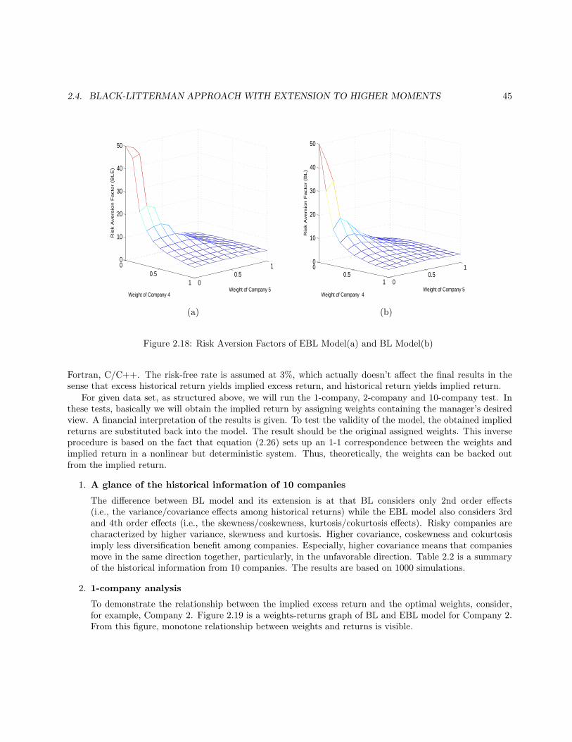
2.4. BLACK-LITTERMAN APPROACH WITH EXTENSION TO HIGHER MOMENTS 45
00.5
1 00.5
10
10
20
30
40
50
Weight of Company 5Weight of Company 4
Ris
k A
ve
rsio
n F
acto
r (B
LE
)
00.5
1 00.5
10
10
20
30
40
50
Weight of Company 5Weight of Company 4
Ris
k A
ve
rsio
n F
acto
r (B
L)
(a) (b)
Figure 2.18: Risk Aversion Factors of EBL Model(a) and BL Model(b)
Fortran, C/C++. The risk-free rate is assumed at 3%, which actually doesn’t affect the final results in thesense that excess historical return yields implied excess return, and historical return yields implied return.
For given data set, as structured above, we will run the 1-company, 2-company and 10-company test. Inthese tests, basically we will obtain the implied return by assigning weights containing the manager’s desiredview. A financial interpretation of the results is given. To test the validity of the model, the obtained impliedreturns are substituted back into the model. The result should be the original assigned weights. This inverseprocedure is based on the fact that equation (2.26) sets up an 1-1 correspondence between the weights andimplied return in a nonlinear but deterministic system. Thus, theoretically, the weights can be backed outfrom the implied return.
1. A glance of the historical information of 10 companies
The difference between BL model and its extension is at that BL considers only 2nd order effects(i.e., the variance/covariance effects among historical returns) while the EBL model also considers 3rdand 4th order effects (i.e., the skewness/coskewness, kurtosis/cokurtosis effects). Risky companies arecharacterized by higher variance, skewness and kurtosis. Higher covariance, coskewness and cokurtosisimply less diversification benefit among companies. Especially, higher covariance means that companiesmove in the same direction together, particularly, in the unfavorable direction. Table 2.2 is a summaryof the historical information from 10 companies. The results are based on 1000 simulations.
2. 1-company analysis
To demonstrate the relationship between the implied excess return and the optimal weights, consider,for example, Company 2. Figure 2.19 is a weights-returns graph of BL and EBL model for Company 2.From this figure, monotone relationship between weights and returns is visible.
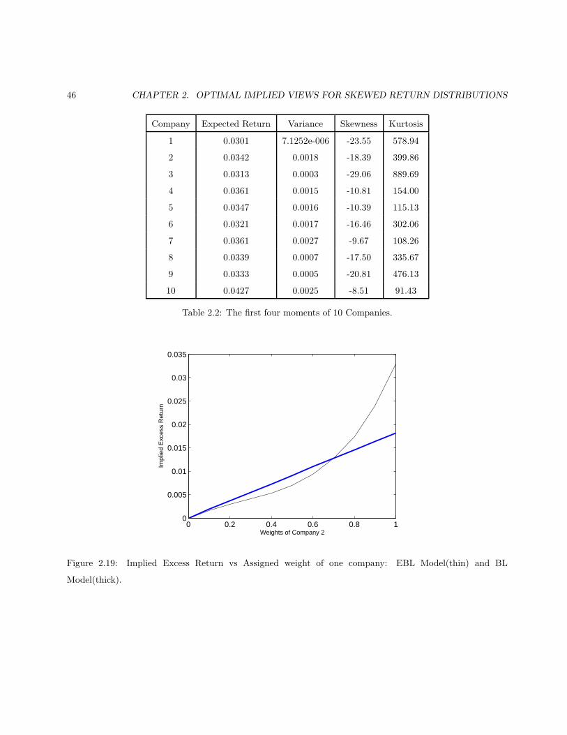
46 CHAPTER 2. OPTIMAL IMPLIED VIEWS FOR SKEWED RETURN DISTRIBUTIONS
Company Expected Return Variance Skewness Kurtosis
1 0.0301 7.1252e-006 -23.55 578.94
2 0.0342 0.0018 -18.39 399.86
3 0.0313 0.0003 -29.06 889.69
4 0.0361 0.0015 -10.81 154.00
5 0.0347 0.0016 -10.39 115.13
6 0.0321 0.0017 -16.46 302.06
7 0.0361 0.0027 -9.67 108.26
8 0.0339 0.0007 -17.50 335.67
9 0.0333 0.0005 -20.81 476.13
10 0.0427 0.0025 -8.51 91.43
Table 2.2: The first four moments of 10 Companies.
0 0.2 0.4 0.6 0.8 10
0.005
0.01
0.015
0.02
0.025
0.03
0.035
Weights of Company 2
Impl
ied
Exc
ess
Ret
urn
Figure 2.19: Implied Excess Return vs Assigned weight of one company: EBL Model(thin) and BL
Model(thick).

2.4. BLACK-LITTERMAN APPROACH WITH EXTENSION TO HIGHER MOMENTS 47
Company Weights Implied Return (EBL) % of Implied Return
4 1 0.0062 1.0112
5 0 0.0002 0.0392
Table 2.3: Manager 1 — Implied Return for heavy weight on company 4 and 0 weight on company 5 (Calibrated
λEBL = 4.9093).
Company Weights Implied Return (EBL) % of Implied Return
4 0 0.0001 0.0199
5 1 0.0049 1.0314
Table 2.4: Manager 2 — Implied Return for heavy weight on company 5 and 0 weight on company 4 (Calibrated
λEBL = 4.5711)
3. 2-company analysis
For the 2-company analysis, consider Company 4 and company 5. The moments of historical returnsare given in Table 2.2. The calculated covariance is 0.000038, which implies the relation of these twocompanies can be ignored. From Table 2.2, Company 4 has higher historical return and lower risk,measured by variance, as compared with Company 5. Consider the following two portfolio determinedby managers with different preference.
Table 2.3 and 2.4 illustrate that Manager 1 is more risky averse as compared with Manager 2 sinceManager 2 invests heavily on a company that has low historical return. We see that λEBL for Manager1 is larger than those for Manager 2. Comparing the implied return under EBL model between the twomanagers, Manager 2’s implied excess returns of Company 5 is larger than those for manager 1. Thismakes sense since Manager 2 invests in a riskier company, implied by higher variance, thus naturally heasks for higher compensation. All of the implied excess returns are positive, which implies a higher ratethan the risk-free rate. Since both managers invested all their money in these two risky companies andno money in the treasury, which is considered risk free, only a higher-than-risk-free-rate will supportsuch an action.
Now, consider two managers who invest partially in companies and the rest at the risk-free rate. Let’sconsider two middle group managers. As expected, Manager 4 is more risk averse since he would ratherinvest in companies than invest at risk-free rate. Company 4 has higher implied excess returns ascompared with Company 5 for both managers since Company 4 is the one that both managers investmost money on.
4. 10-company analysis
The 10 companies used in Section 2 and Section 3 are analyzed. The moments information of historicalreturns are given in Table 2.2.

48 CHAPTER 2. OPTIMAL IMPLIED VIEWS FOR SKEWED RETURN DISTRIBUTIONS
Company Weights Implied Return (EBL) % of Implied Return
4 0.5 0.0062 1.0112
5 0.0 0.0002 0.0393
Table 2.5: Manager 3 — Implied Return for 50% weight on company 4 and 0 weight on company 5, and the
remaining weights on risk-free rate (Calibrated λEBL = 9.8186)
Company Weights Implied Return (EBL) % of Implied Return
4 0.7 0.0065 1.0499
5 0.2 0.0018 0.3817
Table 2.6: Manager 4 — Implied Return for 70% weight on company 4 and 20% weight on company 5, and
remaining 10% on risk-free rate (Calibrated λEBL = 7.1401).
The analysis results are listed in Table 2.7 and Table 2.8. Manager 5 is more conservative since hediversifies his portfolio instead of investing in just a few companies. Thus, his risk aversion factor ishigher. Implied returns are pretty uniform for Manager 5, while for Manager 6, the implied return ofCompany 2, which he invests in the most, is higher.
5. Back testing
Since the BL and EBL models map the weights to the returns through a nonlinear relationship, the opti-mal weights can be recovered if the implied excess returns are used as the inputs. In this test, we incorpo-rate our model with the non-linear solver provided by Matlab, including historical variance/covariance,skewness/coskewness, and kurtosis/cokurtosis of the returns together with the calibrated parameter λ.Weights recovered are consistent with the forward scheme.
2.4.3 Conclusion
The BL and EBL models provide an efficient approach to facilitate the allocation of assets in active hedge fundusing invertible mapping from the implied excess return to the optimal weights. The EBL model, however,is more reliable since it involves high-order moments. Both the forward and backward scheme are verified onthe simulated data provided by Bank of America.

2.4. BLACK-LITTERMAN APPROACH WITH EXTENSION TO HIGHER MOMENTS 49
Company Weights Implied Return (EBL) % of Implied Return
1 0.1 0.0000 0.0629
2 0.1 0.0061 1.4328
3 0.1 0.0005 0.3988
4 0.1 0.0024 0.3898
5 0.1 0.0026 0.5405
6 0.1 0.0052 2.3673
7 0.1 0.0040 0.6354
8 0.1 0.0012 0.3064
9 0.1 0.0007 0.2264
10 0.1 0.0044 0.3395
Table 2.7: Manager 5 — Implied returns when equally 10% weights on all 10 companies (Calibrated λEBL =
18.6232).
Company Weights Implied Return (EBL) % of Implied Return
1 0.0 -0.0000 0.0243
2 0.8 0.0044 1.0564
3 0.0 0.0000 0.0115
4 0.0 0.0002 0.0267
5 0.0 0.0001 0.0162
6 0.0 0.0025 1.1397
7 0.0 0.0002 0.0263
8 0.0 0.0001 0.0183
9 0.0 0.0001 0.0165
10 0.0 0.0001 0.0149
Table 2.8: Implied returns when equally 10% weights on all 10 companies (Calibrated λEBL = 3.5456).

50 CHAPTER 2. OPTIMAL IMPLIED VIEWS FOR SKEWED RETURN DISTRIBUTIONS
2.5 Conclusion
We conclude this paper by comparing the solutions to the model problem obtained by the minimizing CV aRmethod (task 1), the minimizing TE method (task 2), and finally the ELB approach (task 3). Recall themodel problem: given the vector of weights w(i) = 0.1 for 1 ≤ i ≤ 10, the benchmark vector, rb ∈ R400×1, ofthe first 400 scenarios, and the return matrix, R ∈ R400 × R10, of the first 400 scenarios and 10 companies,find how the return matrix must change in order to “optimize” the portfolio return.
1 2 3 4 5 6 7 8 9 100
0.5
1
1.5
2
2.5
3
3.5
4
4.5
Company
Impl
ied
Ret
urn
Mul
tiplie
r
task1task2task3
Figure 2.20: Returns Calculated By Each of the Three Methods
The results are give in Figure 2.20. For each method the graph indicates by what factor the return mustincrease or decrease to obtain an optimal portfolio. As the plot indicates tasks 1 and 2 obtain similar solutions,but task 3 does not follow the same trend. The similarity is not surprising, but neither is the discrepancy. Thisis because in each of the tasks there is a different definition of optimal. For task 1 optimal means minimizingCV aR, in task 2 it is minimizing the tracking error, and in task 3 it is maximizing the utility function. Eachsolution is correct. It is the views of the portfolio managers that must decided what definition of optimal isoptimal.

Bibliography
[1] Black, F. and Litterman, R. (1990) Asset Allocation: Combining Investor Views with Market Equilium,Working Paper, Goldman Sachs, Fixed Income Research.
[2] Martellini, L., Vaissie, M., and Ziemann V.(1999) Investing in hedge funds: adding value through activestyle allocation decision, Edhec Risk and Asset Management Research Center Publication.
[3] Hwang, S. and Satchell, S. (1999) Modelling Emerging Risk Premia Using Higher Moments, InternationalJournal of Finance and Economics, 4:271-296.
[4] Jondeau, E. and Rockinger, M. (2004) Optimal Portfolio Allocation Under Higher Moments, Bank ofFrance Working Papers, 108.
51

52 BIBLIOGRAPHY

Chapter 3
State Vector Estimation in Presence of
Bias
Alvaro Guevara1, Mandar Kulkarni2, Wanying Li3, Wenjin Mao4, Brent Morowitz5, Nebojsa Murisic6
Problem Presenter:Jon C. Kennedy
Lincoln Laboratory, MIT
Faculty Consultants:Dr. Alina Chertock and Dr. Negash Medhin
North Carolina State University
Abstract
Optical sensors have long been part of satellite tracking systems. Imaging telescopes using optical sensors are
well suited for detecting unknown spacecraft, ballistic objects, space debris etc. up to geostationary distances.
The deployment of imaging telescopes in tracking requires one to solve the following inverse problem. Given a
set of angular measurements θk, φk, tk find the best approximation of the vector state ~ψ(t) = (x(t), x(t)) of
1Louisiana State University2University of Alabama at Birmingham3North Carolina State University4University of Colorado at Boulder5Georgetown University6New Jersey Institute of Technology
53

54 CHAPTER 3. STATE VECTOR ESTIMATION IN PRESENCE OF BIAS
the ballistic object. If the exact equations governing the motion of the object are known, as is usually the case,
the inverse problem reduces to merely finding the initial state (x(t0), x(t0)).In this project we have attempted to solve the aforementioned inverse problem by re-formulating it as
an error minimization problem. Two approaches, one involving linearization of the residual vector, and theother using differential evolution were implemented and the results obtained with the two methods compared.A weighted least squares method was developed for noisy measurements. For measurements with noise andperiodic bias, approaches like fast Fourier transforms and low-pass filter design were investigated for removalof the periodic bias from the measurements.
3.1 Introduction and Motivation
Satellites play a very important role in our daily lives, ranging from TV and radio transmission, GPS coordinatedetermination to weather forecasting. In this project, a very important task concerning satellites is studied,namely, determination of its orbital elements. The simplest model to describe the motion of an artificialsatellite around the Earth is the so-called two-body model, a second order ODE, which is fully described inthe next section. Even though more complicated models are used in practice to achieve a higher level ofprecision, the two-body model gives a reasonable approximation. This is due to the fact that the magnitudesof other forces are usually very small compared to the magnitude of the gravitational force produced by theEarth’s mass. The two-body model being a well-posed second order ODE, the problem of determining thelocation of the satellite at all times is thus reduced to the determination of its initial position and velocity.
In our study we try to find the initial state (position and velocity) using a time-stamped set of angularmeasurements provided by an optical sensor. The angular measurements (θk, φk) alone are clearly notsufficient to uniquely determine the initial position of the object because of the freedom in the radial direction.However, time-stamping encodes angular velocity information in the data and the physics (two-body model)constrains the orbit of the object. Thus, in principle, this is a well-posed problem. The challenge stems fromthe fact that the measurements may contain some noise and bias. Furthermore, it is likely that there is no apriori knowledge of the type of noise or bias in the data.
3.2 Mathematical Framework
In this section we develop the mathematical framework for the problem. We assume the two-body model forearth and the satellite. Furthermore, we assume that earth is spherically symmetric, and the mass of thesatellite is negligible compared to that of the Earth. Using Newton’s law of gravity, the acceleration r of thesatellite is given by
r = −GM⊕
r3r (3.1)
where the fraction −r
rdenotes a unit vector pointing towards the center of the Earth,
G = (6.67259± 0.00085) · 10−11m3kg−1s−2
is the gravitational constant and

3.2. MATHEMATICAL FRAMEWORK 55
M⊕ = (5.974) · 1024kg
is the mass of the Earth. In terms of the Euclidean coordinates
r(t) = (x(t), y(t), z(t))
The fact that the force exerted on the satellite always points to the Earth’s center in the the two-body problemhas the immediate consequence that the orbit is confined to a fixed plane for all times. Mathematically, thisamounts to r × r being a constant vector.
The second order ODE described by equation 3.1 can be written as a system of first order equations bythe introduction of an auxiliary variable u. This can be done as follows:
r = u
u = −GM⊕
r3r
(3.2)
The advantage of writing the ODE in equation 3.1 as a system described by equation 3.2 is that the latter isamenable to numerical solution. The initial state determination problem can now be algorithmically describedas follows
(i) Construct the state vector to include, both, the satellite’s position and velocity.
s(t) =
x(t)y(t)z(t)x(t)y(t)z(t)
(ii) Start with a guess for the initial state vector,
s(0)guess = (x(0)guess, y(0)guess, z(0)guess, x(0)guess, y(0)guess, z(0)guess)
and compute the trajectory numerically by solving the ODE described by equation 3.2 subject to theinitial condition given by s(0)guess.
(iii) Obtain the modeled angular measurements from the computed trajectory by a change of variables.
(iv) Calculate the square of the error between modeled observations and actual measurements, i.e. computeJ(s(0)guess) where,
J(s(0)) =
N∑
i=1
(g1 f(s(0), ti) − θi)2 + (g2 f(s(0), ti) − φi)
2
f is the solution of the ODE system subject to the initial conditions given by s(0) and g1 and g2 are themappings on R3 that map (x, y, z) to the spherical co-ordinates θ and φ respectively.

56 CHAPTER 3. STATE VECTOR ESTIMATION IN PRESENCE OF BIAS
(v) Determine the optimal initial state vector by minimizing J .
The last step is critical, as it requires minimization of a non-linear (and possibly non-convex) function. Thefollowing two minimization approaches were investigated.
(a) First an iterative process based on a linearization of the residual vector is considered. The residualvector is obtained as difference between modeled observations and actual measurements.
(b) The second, inspired by genetic algorithms, is the so-called Differential evolution method.
The advantages and drawbacks of each approaches will be commented on in later sections. As a secondstage of the project, noise was considered and the main change in the strategy was to implement a weightedleast squares method. Finally, testing of our procedures is done under the presence of periodic bias.
3.3 Linearization
3.3.1 Linearized Least Squares
The practical solution of the least-squares orbit determination problem is complicated by the fact that h = gfis a highly non-linear function of the unknown vector x0, which makes it difficult or impossible to locate theminimum of the loss function without additional information. An approximate value xapr
0 of the actual epochstate is however, often known, from preliminary orbit determination considerations. We linearize all quantitiesaround a reference state xref
0 , which is initially given by xapr0 , the residual vector is approximately given by
ρ = z − h(x0)
≈ z − h(xref0 ) − ∂h
∂x0(x0 − xref
0 )
= z −Hx0 (3.3)
Here
x0 = x0 − xref0
denotes the difference between x0 and the reference state, while
z = z − h(xref0 )
denotes the difference between the actual observations and the observations predicted from the referencetrajectory. Furthermore, the Jacobian
H =∂h(x0)
∂x0
∣∣∣∣x0=xref
0
gives the partial derivatives of the modeled observations with respect to the state vector at reference epoch t0.Using the above abbreviations, equation 3.3 provides a prediction of the measurement residual after applyinga correction x0 to the reference state and recomputing the modeled observations h.

3.3. LINEARIZATION 57
The orbit determination problem is now reduced to the linear-least squares problems of finding xlsq0 such
that
J(x0) = (z −Hx0)T (z −Hx0)
i.e. the predicted loss function after applying a corrections x0 becomes a minimum. If the Jacobian hasfull rank m, i.e. if the columns of H are linearly independent, this minimum is uniquely determined by thecondition that the partial derivatives of J with respect to x0 vanish:
∂(z −Hx0)T (z −Hx0)
∂x0
∣∣∣∣x0=xlsq
0
= 0.
Using the relation
∂aT b
∂c= aT ∂b
∂c+ bT
∂a
∂c
to compute the derivatives of ρTρ, the general solution of the linear least-squares problem may be written as
xlsq0 = (HTH)−1(HTz)
after a proper rearrangement.Due to the non-linearity of h, the simplified loss function differs slightly from the rigorous one and the
value of xlsq0 = xref
0 +xlsq0 determined so far is not yet the exact solution of the orbit determination problem.
It may, however, be further improved by substituting it for the reference value xref0 and repeating the same
procedure. Based on this idea the non-linear problem is solved by an iteration
xj+10 = xj
0 + (HjTHj)−1HjT (z − h(xj0)) (3.4)
which is started from x00 = xapr
0 and continued until the relative change of the loss function is smaller than aprescribed tolerance for successive approximations. The Jacobian
Hj =∂h(x0)
∂x0
∣∣∣∣x0=xj
0
is updated in each iteration to ensure an optimum convergence. Even though the number of iterations increasesin this case, the total computational effort is reduced, due to the high amount of work that is otherwise requiredfor the integration of the state transition matrix.
3.3.2 Weighted Least Squares
The algorithm developed in the previous section depends on equal weighting of all observations. However,if the measurements are composed of different types of accuracies, a weighting has to be introduced. Eachobservation is weighted with the inverse of the mean measurement error σi, i.e. by replacing the residuals ρi
with the normalized residuals
ρi =1
σi=
1
σi(zi − hi(x0)).

58 CHAPTER 3. STATE VECTOR ESTIMATION IN PRESENCE OF BIAS
Here σi considers the total expected error in the measurement due to both random noise and systematic errors.As a result the basic least-squares equation
xlsq0 = (HT H)−1(HTz)
remains essentially unchanged, except that H and z are replaced by the modified values
H = SH and z = Sz
Here S is a square diagonal matrix
S = diag(σ−11 , · · · , σ−1
n ) =
σ−1
1 0. . .
0 σ−1n
which divides the ith row of a matrix or vector by σi upon multiplication from the left.
Alternatively the solution of the weighted least-squares problem may be written as
xlsq0 = (HTWH)−1(HTWz)
using the weighting matrix
W = S2 = diag(σ−11 , · · · , σ−1
n )
The iteration equation 3.4 in the previous section thus changes to
xj+10 = xj
0 + (HjTWHj)−1HjTW (z − h(xj0)) (3.5)
3.4 Differential Evolution for Optimization
Differential evolution is a stochastic parallel direct search evolution strategy optimization method that isfairly fast and reasonably robust. Differential evolution is capable of handling nondifferentiable, nonlinear andmultimodal objective functions. It has been used to train neural networks having real and constrained integerweights.
In a population of potential solutions within an n-dimensional search space, a fixed number of vectorsare randomly initialized, then evolved over time to explore the search space and to locate the minima of theobjective function.
At each iteration, called a generation, new vectors are generated by the combination of vectors randomlychosen from the current population (mutation). The outcoming vectors are then mixed with a predeterminedtarget vector. This operation is called recombination and produces the trial vector. Finally, the trial vectoris accepted for the next generation if and only if it yields a reduction in the value of the objective function.This last operator is referred to as a selection.

3.4. DIFFERENTIAL EVOLUTION FOR OPTIMIZATION 59
0 200 400 600 800 10002.8
2.85
2.9
2.95
3
3.05
3.1
3.15
3.2
Th
eta
Data without Noise or Bias
0 200 400 600 800 10000.2
0.4
0.6
0.8
1
1.2
1.4
1.6
Ph
i
0 200 400 600 800 10002.8
2.85
2.9
2.95
3
3.05
3.1
3.15
3.2Estimates by LSM
0 200 400 600 800 10000.2
0.4
0.6
0.8
1
1.2
1.4
1.6
0 200 400 600 800 1000−6
−4
−2
0
2
4
6x 10
−9 Errors
0 200 400 600 800 1000−1
−0.5
0
0.5
1
1.5x 10
−8
Figure 3.1: Linearized Least Squares Method for Noiseless Data

60 CHAPTER 3. STATE VECTOR ESTIMATION IN PRESENCE OF BIAS
0 200 400 600 800 10002.8
2.85
2.9
2.95
3
3.05
3.1
3.15
3.2
Th
eta
Data with White Noise
0 200 400 600 800 10000.2
0.4
0.6
0.8
1
1.2
1.4
1.6
Ph
i
0 200 400 600 800 10002.8
2.85
2.9
2.95
3
3.05
3.1
3.15
3.2Estimates by LSM
0 200 400 600 800 10000.2
0.4
0.6
0.8
1
1.2
1.4
1.6
0 200 400 600 800 1000−8
−6
−4
−2
0
2
4
6
8x 10
−6 Errors
0 200 400 600 800 1000−1.5
−1
−0.5
0
0.5
1
1.5
2x 10
−5
Figure 3.2: Linearized Least Squares Method for Data with White Noise

3.4. DIFFERENTIAL EVOLUTION FOR OPTIMIZATION 61
0 200 400 600 800 10002.8
2.85
2.9
2.95
3
3.05
3.1
3.15
3.2
Th
eta
Data with Noise and Bias
0 200 400 600 800 10000.2
0.4
0.6
0.8
1
1.2
1.4
1.6
Ph
i
0 200 400 600 800 10002.8
2.85
2.9
2.95
3
3.05
3.1
3.15
3.2Estimates by LSM
0 200 400 600 800 10000.2
0.4
0.6
0.8
1
1.2
1.4
1.6
0 200 400 600 800 1000−4
−3
−2
−1
0
1
2
3
4x 10
−5 Errors
0 200 400 600 800 1000−5
−4
−3
−2
−1
0
1
2
3
4
5x 10
−5
Figure 3.3: Linearized Least Squares Method for Data with White Noise and time varying bias

62 CHAPTER 3. STATE VECTOR ESTIMATION IN PRESENCE OF BIAS
0 200 400 600 800 10002.8
2.85
2.9
2.95
3
3.05
3.1
3.15
3.2Data with White Noise
Th
eta
0 200 400 600 800 10000.2
0.4
0.6
0.8
1
1.2
1.4
1.6
Ph
i
0 200 400 600 800 10002.8
2.85
2.9
2.95
3
3.05
3.1
3.15
3.2Estimates by Weighted Least Squares
0 200 400 600 800 10000.2
0.4
0.6
0.8
1
1.2
1.4
1.6
0 200 400 600 800 1000−8
−6
−4
−2
0
2
4
6
8x 10
−6 Errors
0 200 400 600 800 1000−2
−1.5
−1
−0.5
0
0.5
1
1.5
2x 10
−5
Figure 3.4: Weighted Least Squares Method for Data with White Noise

3.4. DIFFERENTIAL EVOLUTION FOR OPTIMIZATION 63
0 200 400 600 800 10002.8
2.85
2.9
2.95
3
3.05
3.1
3.15
3.2Data with Noise and Bias
Th
eta
0 200 400 600 800 10000.2
0.4
0.6
0.8
1
1.2
1.4
1.6
Ph
i
0 200 400 600 800 10002.8
2.85
2.9
2.95
3
3.05
3.1
3.15
3.2Estimates by Weighted Least Squares
0 200 400 600 800 10000.2
0.4
0.6
0.8
1
1.2
1.4
1.6
0 200 400 600 800 1000−4
−3
−2
−1
0
1
2
3
4x 10
−5 Errors
0 200 400 600 800 1000−6
−4
−2
0
2
4
6x 10
−5
Figure 3.5: Weighted Least Squares Method for Data with White Noise and Time Varying Bias

64 CHAPTER 3. STATE VECTOR ESTIMATION IN PRESENCE OF BIAS
0 200 400 600 800 10002.8
2.85
2.9
2.95
3
3.05
3.1
3.15
3.2
Th
eta
Data without Noise
0 200 400 600 800 10000.2
0.4
0.6
0.8
1
1.2
1.4
1.6
Ph
i
0 200 400 600 800 10002.8
2.85
2.9
2.95
3
3.05
3.1
3.15
3.2Estimates
0 200 400 600 800 10000.2
0.4
0.6
0.8
1
1.2
1.4
1.6
0 200 400 600 800 1000−6
−4
−2
0
2
4
6x 10
−9 Errors
0 200 400 600 800 1000−1
−0.5
0
0.5
1
1.5x 10
−8
Figure 3.6: Differential Evolution for Noiseless Data

3.5. RESULTS 65
Test Case r1 in m. r2 in m. r3 in m. v1 in m/s. v2 in m/s. v3 in m/s. l2 Error
x0 -6878132.2 1487.636 7548.473 8.965 986.073 7548.469
Data D.E. -6878132.1 1487.634 7548.462 8.965 986.073 7548.469
Without error -0.1038 0.0015 0.0104 0.0001 5.69 × 10⁻⁶ 4.73 × 10⁻⁵ 0.104
Noise or L.S. -6878132.1 1487.634 7548.461 8.965 986.073 7548.469
Bias error -0.1127 0.0015 0.0114 0.0001 6.51 × 10⁻⁶ 5.00 × 10⁻⁵ 0.113
Data L.S. -6878172.9 1487.223 7522.119 9.023 986.075 7548.489
With error 40.642 0.412 -3.645 -0.058 −0.002 -0.019 40.807
White W.L.S. -6878189 1484.859 7550.543 9.037 986.080 7548.512
Noise error 56.821 2.776 -2.070 -0.072 -0.006 -0.042 56.926
Data with L.S. -6877599.4 1477.787 7520.531 8.236 986.038 7548.205
White Noise error -532.820 9.847 27.941 0.728 0.034 0.264 533.644
& Time W.L.S. -6877360 1472.672 7593.816 7.868 986.036 7548.157
Varying bias error -772.241 14.963 56.656 1.097 0.037 0.311 7743.18
Table 3.1: Performance of algorithms for various data sets.
3.5 Results
In this section we present the results of a simulation and comments on this are provided. Orbital data wascreated by using MATLAB ODE solver with the initial condition
s(0) = (−6878132.2, 1487.636, 7548.473, 8.965, 986.073, 7548.469)
Then, the resulting data is converted into angular measurements, using spherical coordinates. An initialguess is chosen, and the least square (L.S.) and differential evolution (D.E.) methods are used to computethe approximation. To simulate data corrupted by white noise an extraneous noise is added, and least squaremethod is compared to the weighted least square (W.L.S.). Finally, some bias is added to the measurementsand we compare these methods again, as reported in the next table.
For the noiseless and unbiased data, we obtain a very small error with both methods. The D.E. methodseems to give a higher level of accuracy, a remarkable fact, considering that, in its heart, it is random searchbased. However, computationally, it is more expensive than L.S. Also, both methods showed small sensitivityto changes in the initial conditions. As a trend, though, for L.S. it usually took more iterations to providethe result, as for D.E. method, the initial condition change demanded longer computational time. Moreover,as for the results of L.S. and W.L.S. approaches , even when L.S. renders a smaller error, W.L.S. is suggestedin the presence of noise due to its robustness. In the presence of bias, both methods deliver a higher error, asexpected.

66 CHAPTER 3. STATE VECTOR ESTIMATION IN PRESENCE OF BIAS
3.6 Future directions
As a starting point, we have done some preliminary investigations for removal of the bias in measurementassuming the bias is bounded and periodic. Periodic bias assumption is not unreasonable due to the natureof the data collection process and in this case, it is said that the data “rides on a periodic wave”. Spectralmethods like Fourier transforms or low pass filter can be used to “filter-out” unwanted frequencies in the data.Then we have reduced the problem to data with noise on which our algorithms perform reasonably well.
Another important issue to address is the computation of the covariance matrix in the presence of bias.The covariance matrix is important as it determines a volume around the estimated initial condition wherethere is a certain probability (usually 95 percent is chosen) to find the actual satellite position. In the unbiasedcase, there are explicit formulas to compute this covariance matrix. However, it is unclear how to introducethe possible filter effect in the covariance matrix when bias is considered.
The next conjecture we have for improving algorithm performance stems from the fact we often encounterednumerical singularities even after the problem was reasonably scaled. Also, the methods are computationallysomewhat expensive. It is conjectured that by modifying the function J to include the time-derivative infor-mation encoded in the data, better performance, can be expected. We propose to use the function J ′ insteadof J where the former is defined as:
J(s(0)) =
N∑
i=1
(g1 f(s(0), ti) − θi)2 + (g2 f(s(0), ti)− φi)
2 + (g1 f ′(s(0), ti) − θ′i)2 + (g2 f ′(s(0), ti)− φ′i)
2
where prime denotes differentiation with respect to time. This idea has been developed and applied to a lotof interesting real-world problems by J. Neuberger in [4].
It would also be of interest to investigate if by fusing two sets of measurements obtained by two differentsensors a better estimate of the initial state can be obtained.

Bibliography
[1] Montenbruck, O. and Gill, E. (2000) Satellite Orbits : Models, Methods and Applications, Springer-Verlag,Heidelberg.
[2] Tapley, B., Schutz, B. and Born, G. (2004) Statistical Orbit Determination, Elsevier Academic Press,London.
[3] Sagan, H. (1992) Introduction to The Calculus of Variations, Dover Publications, INC., New York.
[4] Neuberger, J. Sobolev Gradients and Differential Equations, Preprint
67

68 BIBLIOGRAPHY

Chapter 4
Planning Problem Involving Resource
Constraints
Sergei Belov1, Ye Chen2, Aneesh Hariharan3, David King4, Jenny Law5, Ting Wang6
Problem Presenter:Pierre F. Maldague
Jet Propulsion LaboratoryNASA
Faculty Consultant:Kartik Sivaramakrishnan
North Carolina State University
Abstract
Modern space missions (Galileo, Cassini, and MER Expedition) conducted by NASA require the execution ofa number of activities subject to available resources. Some of the resources like electric power and computermemory are replenishable. Each activity requires a time window for its execution and some activites canconceivably be performed in parallel. The objective in the space mission is to order/schedule the variousactivities so as to minimize the time taken to complete the space mission. We develop a heuristic algorithm
1Duke University2Clarkson University3Auburn University4Arizona State University5Duke University6Kansas State University
69

70 CHAPTER 4. PLANNING PROBLEM INVOLVING RESOURCE CONSTRAINTS
for this problem in this paper and have implemented it in MATLAB. Preliminary computational results withthe algorithm on test instances indicate that it is both fast and robust.
4.1 Introduction
In space operations a satellite or a space vehicle is equipped to perform several operations [1]. But verytypically these operations are constrained by a fixed set of un-replenishable resources. For example in theGalileo mission (Oct 18, 1989) to Jupiter [2], the spacecraft did not have enough fuel to fly directly to Jupiter,but the mission succeeded nevertheless because the spacecraft borrowed energy from Earth and Venus’s gravityand pulled along. Similarly during its flight after passing earth, its umbrella shaped high gain antenna did notopen and once again the mission succeeded in sending the original expected data since a smaller antenna wasused to send back the data. Here and in various other missions such as Cassini [3] and the Mars ExplorationRover (MER) Mission [4], the role of planners and planning has become inevitable since every space mission’sactivities is constrained by a number of resources, both known and unknown. For example, in the abovementioned Galileo expedition, it was planning under resource constraints that had led to a flight plan VEEGA-Venus-Earth-Earth Assisted Gravity that aided Galileo to soar past Venus and twice past Earth, thus aidingit to gain enough momentum to travel up to Jupiter. In every space exploration mission, associated witheach activity is a set of resources and constraints, which have to be thought of and planned for. For example,every spacecraft has a fixed amount of fuel for maneuvering so any maneuvering operation is constrained bya fixed amount of fuel. The electrical power required for various electrical equipment (computers, Radars,transmitters) etc. is constrained by the electrical output provided by the solar panels. The CPU size isconstrained by the size of the computer and the fact that the computer must be designed to withstand solarwind/radioactivity and large magnetic fields. In general we may model the spacecraft as a machine designedto perform certain tasks or activities, wherein each activity consumes a certain amount of a fixed resource andthis resource is either replenishable or non-replenishable. Examples of replenishable resources are electricalpower and computer memory as electrical power can always be replenished by the solar panels, and computermemory can be recovered by removing files from stored memory. Examples of non-replenishable resources arepropellant where once we use this resource the resource is gone. Typically most operations on board a spacevehicle involve activities of the replenishable type.
Once the set of activities and resource constraints are known, the problem does not end there. Thereshould be a way of efficient scheduling of activities, since a serial execution of each of these would lead to awastage of a lot of resources, which is unwarranted. Our task is to produce a method to optimize the timeto complete a fixed set of necessary activities, while simultaneously remaining under a fixed set of resourceconstraints. While this type of a planning problem seems initially to be quite simple and understandable, thisis a problem that NASA continually has to deal with due to the remote nature of the satellite. Also we need torealize that a satellite is at quite some distance from earth, so if anything goes wrong it is impossible to rectifydue to the satellite’s distance from earth. As it turns out and as we get into the mathematics of the problemof optimization of discrete time events under the presence of linear constraints, we end up in a non-trivialexercise. Typically there are a much larger number of constraints compared to the number of activities.
When our team started programming our algorithm, we decided to confine ourselves to the case of re-plenishable resources. In our model we utilized the scheduling of non-consumable activities because this wasthe simple case. And since we succeeded in this, we quickly realized that the same algorithm with slightmodification could be utilized to deal with the case of consumable resources. A series of tasks that can beachieved as a direct consequence of our algorithm have also been enlisted.

4.2. PRELIMINARIES 71
4.2 Preliminaries
4.2.1 Definitions and explanation of terms
Resource: A Resource is a source of aid or support that may be drawn whenever needed (source: WebDefinition). Ex. Power, Data Volume, Battery State of Charge etc. The resources form the constraints inour problem. There are two types of resources (a) Consumable resources: These kind of resources are notreplenished at the end of an activity. Ex: Rocket propellant (b) Non Consumable Resources: These kind ofresources are replenished at the end of an activity. Ex: Electric Power (can be replenished with the use ofsolar panels)
Activity Type: An activity type is a task that a space exploration mission is expected to achieve. Ex.Telecom, CPU ,Radar, Imaging, Chemical Analysis. Every activity type is constrained by an amount ofresource that it consumes. An activity type can be performed more than once in an exploration.
Frequency: The frequency of an activity type is the number of times the particular activity type is performed.Ex. If the frequency for imaging is 3, it means that 3 imaging operations are performed during the mission.
Duration: The duration of an activity type is the time required to finish the activity type under consideration.
Resource Matrix: A Resource Matrix is a matrix with the activity types as the column elements and theresources as the row elements. The entries in the matrix represent the amount of resources that each activitytype consumes. Ex: If Imaging consumes 70 percent of power and radar consumes 80 percent of power, thenthe Resource Matrix is 1x2 matrix with entries 70 and 80.
Plan: A plan is a set of activities performed taking into account the resources under which they are limited.An activity performed as part of plan is expected to be defined by its start time, its end time and its type.
Optimal plan: An optimal plan is a plan with the minimal total time to perform all the activities of amission under the set of resource constraints.
Overlap: Overlap is the amount of time two activity types are performed in parallel compared to the totaltime of these two activity types. In case two activities are incompatible, the overlap is 0. We assume twoactivities of the same type have an overlap of 0.
Thread: The number of threads in a plan signify the number of parallel activities that are feasible. Thenumber of threads could be less than the number of activity types, except that we would be moving away fromthe optimal solution. Ex. If all the activities are performed serially i.e. there are no parallel computations,the number of threads is 1.
Compatible activity types: Any set of activity types are said to be compatible if the resource consumed byeach of them adds up to a number, which is less than the maximum amount that the particular resource typecan have. Typically this maximum value is 100 percent. Ex: If Imaging consumes 70 percent of the availablepower, Radar consumes 80 percent of the available power and Chemical Analysis consumes 20 percent of theavailable power, then activity types Imaging and Chemical Analysis and Radar and Chemical Analysis areindividually said to be compatible with each other whereas Imaging and Radar as far as the power resourcegoes, are said to be incompatible with each other. With respect to the resource constraint matrix, if the sumof a set of column entries in a particular row exceeds 100, the whole set is said to be set of incompatibleactivity types. However, they could be pairwise compatible or triple compatible etc.
Rule of Thumb: The Rule of Thumb matrix is a hypothetical matrix that consist of only 0’s and 1’s as itentries and resembles the behavior or the resource matrix to the largest possible extent.

72 CHAPTER 4. PLANNING PROBLEM INVOLVING RESOURCE CONSTRAINTS
4.2.2 Problem Description
Given a set of activities, resources and the resource matrix, how can we best schedule the set of activities sothat the time required to complete the proposed plan is minimized? What are the corresponding set of nearlyoptimal plans that minimizes the time and what is the value of this time? Once this has been achieved, thenext question that needs to be addressed is how does the convergence of the plan depend on the number ofactivities, the number of resources and the size of the resource matrix? Can we find out the amount of overlapof each of the activities that can occur in parallel in the form of an overlap matrix and if successful what doesthis overlap matrix signify about the Rule of Thumb? Is there any promise for future work by building up onthe proposed ideas?
4.3 Algorithm
Let us illustrate what our algorithm does to optimize the total time of a mission by use of a simple example.Suppose that we have a simple satellite that can perform 3 different types of tasks (N=3) and has threeresource constraints (M=3). Let us assume that our satellite has a Camera, a Transmitter and a Radar forranging. Our activities are therefore Imaging (A1), Telecom (A2), and Ranging (A3) respectively. Supposefor this example the satellites non-consumable resources are Power, CPU, and Data-transfer rate. The matrixbelow contains the percentages that each activity type borrows during operation in units of percentage of totalresource:
Type Imaging Telecom RangingPower (%) 20 90 75CPU (%) 80 90 20Data (%) 60 50 10
(4.1)
That is for example Ranging temporarily uses 75% of Power, 20% of CPU and 10% of Data transferchannel. The above matrix we define to be our resource matrix.
Since we assume that our satellite has only one camera, one transmitter, and one radar only one activityof each type may occur simultaneously. Let us define Ai(t) as a binary variable to be 0 or 1 dependent uponwhether the activity of type i is on or off at time t. Our restriction equations for this satellite are therefore:
0.2A1(t) + 0.9A2(t) + 0.75A3(t) ≤ 1
0.8A1(t) + 0.9A2(t) + 0.2A3(t) ≤ 1
0.6A1(t) + 0.5A2(t) + 0.1A3(t) ≤ 1
for all t ≥ 0.These equations represent the fact that it is not possible to schedule two or more activities which consume
more than maximum available resources (in our example 100%). Analyzing the above matrix we can see thatRanging and Telecom activities cannot occur together as they would for example utilize more power than isavailable. Also Imaging and Telecom activities cannot occur simultaneously as they are constrained by CPUand Data transfer rate. Since we only have one camera, one radar, and one transmitter on our satellite it isnot possible to have more than one imaging, ranging, or transmitting activity occur simultaneously. On theother hand you see from above it is possible to have imaging and ranging activities occur together.

4.3. ALGORITHM 73
Let us suppose that our satellite must perform a certain number of predetermined activities in order forthe mission to be successful. Let Fi be the frequency or the required number of operations for task of type i.For simplicity suppose also that each activity or task of type i has a fixed duration Di.
For illustrative purposes lets choose
F =(
3, 2, 2), D =
(1, 4, 1
)(4.2)
This states that we need to schedule 3 Imaging activities, 2 Telecom activities, and 2 Ranging activities.The mission will be complete when all required activities have been completed. Our task is to minimize thetime required to complete the mission (T). We can think about each activity as a block with given length. Inother words we are looking for an arrangement of 7 blocks which minimizing the total time. Or we want theshortest wall made of these blocks. If the system had no constraints this optimal arrangement would be asfollows: all tasks would be executed in parallel.
This configuration would have 7 threads But this would not satisfy the constraints above. The real taskis to design an algorithm that satisfies the constraints at all times and simultaneously minimizes the time tocomplete this task. This motivates how we designed the algorithm. Ultimately we want to maximize thenumber of threads. So to do this at each step of the way if it is possible to insert a block in a new threadwithout violating our resource constraints we will do so. Here is a block diagram of how the algorithm works.First we randomly choose a block to be inserted at t=0 and thread = 1.
Next as you can see from the diagram (Fig. 4.1) we see if any blocks (or activities) are compatible with thecurrent blocks we just added. The idea is we want to compress as much activity as possible in as little time aspossible. So if we are allowed to put an activity in one more thread we should do so to increase the numberof parallel tasks. First we increase the number of threads as much as possible and then move to next time. Ifthere is more than one type of activity can be allocated at considered spot we make random selection.
Step-by-step this algorithm can be explained as follows: STEP 1: At t = 0 all 3 types available: Imaging,Telecom, Ranging. Suppose the random generator chose type 3 - Ranging.
Next step is to try to add another thread. The list of available types is only one type Imaging - we addit.
Next we still try to add another thread, but the combination Ranging+Imaging uses a lot of resources. Sothe list of compatible types is empty.
Now it is time to update time: we move to the next open right end point and repeat the above procedureagain: build up first, move right by updating time after that.
The following sequence of pictures (Figs. 4.2,4.3) illustrates in a step by step fashion how the programselects blocks.
As you can see since each step along the way we randomly choose an activity type from those which arecompatible it is not hard to see that many different combinations of results are possible. When the number oftypes (N) is small our results indicate that there is little difference in net mission time (T) between repeatedruns of the same algorithm. As the number of types (N) tends to increase we see more differences in missiontimes that the algorithm computes. However there are many different arrangements which produce the sametime T.
If we repeat this algorithm over and over again and select the minimum time of all runs. The minimumtime of L random schedules produced by the algorithm should converge to the true value T ∗ of all possiblecombinations. We argue this claim, since the number of combinations of activity types is finite and since foreach combination of activity types the algorithm minimizes the mission time. We therefore build into ourprogram a process where we may repeat a given random schedule arrangement any given number of times andselect the minimum mission time amongst all runs. In practice we see that it is typical to see little difference
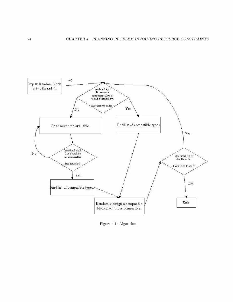
74 CHAPTER 4. PLANNING PROBLEM INVOLVING RESOURCE CONSTRAINTS
Figure 4.1: Algorithm
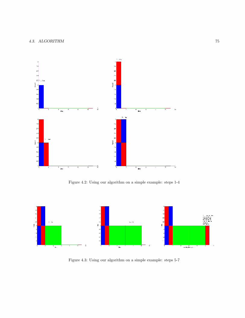
4.3. ALGORITHM 75
Figure 4.2: Using our algorithm on a simple example: steps 1-4
Figure 4.3: Using our algorithm on a simple example: steps 5-7

76 CHAPTER 4. PLANNING PROBLEM INVOLVING RESOURCE CONSTRAINTS
in the minimum value of T once our algorithm has gone through 10 to 20 random iterations even when wehave as much as 100 different activity types. We outline much of these results in the findings section of thispaper.
4.4 Results
Figure 4.4: Simple example with three resources and three types
In this section, we present the results produced by our algorithm described earlier.
1. A simple example
First of all, we go back to the simple example with three resources and three types (imaging, telecomand ranging). Our algorithm runs a hundred trials and finds the plan (out of these trials) with the leastamount of time required to complete.
As we can see, the graph in Fig. 4.4 confirms the fact that imaging and ranging can occur at the sametime.
Next, let us look at the time needed to complete all the activities for each trial. Notice that in Fig. 4.5every trial produces a plan requiring the same time (T = 11) to complete. Thus, for this simple example,our algorithm produces an optimized plan, which is not unique though as shown in Fig. 4.6.
2. A more complicated example
After looking at the simple example earlier, let us look at a more complicated example with 100 resourcesand 100 types of activities. The resource matrix is generated by random with entries being uniformly

4.4. RESULTS 77
Figure 4.5: Time needed for each trial
distributed between 0% and 10%. Durations of these 100 activity types were chosen on random as well -uniformly on [0,1]. And finally we used the all frequencies to be the same: Fi = 20 for all i = 1, ..., 100.The plan produced by our algorithm is shown in Fig. 4.7. Different colors correspond to the differenttypes of activities.
Note that our algorithm is optimizing in some sense, as the plan in Fig. 4.7 shows a short tail at theend. Next, we look at the time needed for plan to complete for each run, for this complicated example.
From Fig. 4.8, we see that the time needed to complete the plan is not the same any more for each ofthe one hundred trials, in this complicated example. But note the fast convergence rate in Fig. 4.9. Wecan see the dramatic decrease of time needed at the beginning of running our trials.
Next, we look at the histogram of the times needed in those one hundred trials. As shown in Fig. 4.10,the most probable time needed is quite close to the minimum time found out of those one hundred trials.
3. Effect of size of resource matrix on the number of threads
Here, we investigate how the number of threads decreases as we increase the average value (of all entries)of the constraint matrix. This makes sense because as we increase value in R, we make more pairs ofactivity types incompatible, thus decreasing the number of threads. We are using 10 activity types and20 resource types generated by random. We also used random durations uniform on [0,1] and Fi = 20for all i = 1, ..., 20. The result is shown in Fig. 4.11. You can see that for small size the resource matrixentries (meaning low resource usage by all activity types) for all activity types are 100% compatible.With the size of R matrix growing, less and less number of potential threads are utilized. At the averageentries of R matrix being approximately 0.4, only one thread out of potential 10 potential threads are inuse meaning that all activities are executed as a sequence without possibility for optimization. Finally

78 CHAPTER 4. PLANNING PROBLEM INVOLVING RESOURCE CONSTRAINTS
Figure 4.6: Another optimized plan for the same simple example
the size of the resource matrix becomes so large that even one thread is is not produced. This signifiesa situation when all of the activity types have too large resource utilization.
Also we try to fit a line to the curve using the function
f(x) =0.0741
x.
This function describes well the curve only on the initial stage. Further investigation is needed to obtaina better model.
4. Measures of pairwise overlaps from the plan
Here, we want to ultimately develop some rules of thumb that can simplify our resource constraintmatrix. As a first step, we form the pairwise overlap matrix S from a plan with minimum time (out of acertain number of trial runs) found by our algorithm. Each entry Si,j in S measures the length of timewhen an activity of type i and an activity of type j overlap, then divided by the length of time takenby the union of activities both of type i and type j. This gives us a sense of how probable it is that anactivity of type i and an activity of type j go together.
For simplicity, we assume for all k, DkFk is approximately constant, where Dk is the duration and Fk isthe frequency for activity of type k. For example, we take F = [2 3 4 5 6 ] and D = [6 4 3 2.4 2]. Andwe take R to be:

4.4. RESULTS 79
Figure 4.7: A more complicated example with 100 resources and 100 types of activities
R =
33.8310 19.0582 38.8168 11.5866 31.999821.9426 1.0509 29.5480 21.4981 26.422214.7475 22.3867 38.7426 14.0382 18.53031.6784 8.1148 42.3460 5.4720 38.030638.4494 35.3126 34.9388 33.3951 0.8647
.
Fig. 4.12 shows a plan produced by our algorithm. We can see that, for example, the activities of typegreen and light green overlap about half of the time; similarly, activities of type purple and light purpleoverlap for one-third of the time. Let us show how the resulting overlap matrix reflects such information:
S =
0 0.5190 0 0.1881 0.33330.5190 0 0.1881 0 0.2500
0 0.1881 0 0.5190 0.33330.1881 0 0.5190 0 0.42860.3333 0.2500 0.3333 0.4286 0
From the histogram for entries in the overlap matrix S, we can see that many entries are zero (Fig. 4.13).This suggests that several pairs here do not overlap. In this way, we can gradually create some rules ofthumb matrix to simplify our problem.
Next, let us look at a more complicated example with a hundred resources and a hundred types ofactivities. Fig. 4.14 shows the plan that our algorithm finds and the histogram for the entries in thecorresponding overlap matrix S (Fig. 4.15). We can see that most entries in S are very small, meaningthat many pairs overlap only for a small fraction of time.

80 CHAPTER 4. PLANNING PROBLEM INVOLVING RESOURCE CONSTRAINTS
Figure 4.8: Time needed for each of the 100 trials
Figure 4.9: Convergence rate

4.5. FUTURE WORK 81
Figure 4.10: Histogram of times needed
4.5 Future work
Our algorithm and solution analyze only non-consumable resources. This work can be furthered on to theallocation of activities under consumable resource constraints or a combination of both, which would thengive a complete outline of planning activities for any mission. This problem would be a slight modification ofour algorithm by making sure that at the end of every activity, we subtract the resource consumed from theinitial value for resources of type consumable and incorporate it in the algorithm.
• We could incorporate science values in our algorithm, which assign a preference to one particular activityover another. The complexity of the algorithm is bound to increase since besides the resource constraints,we have to keep in mind the weights attached to the execution of an activity. However the situationrepresents a more real time problem and its worth tackling.
• Sometimes certain activities (e.g. telecom) need specific ’windows’ for their execution and no otheractivity should hinder their performance in their window of opportunity. So, we could try and incorporatethis idea in our algorithm to give credence to various activities with priorities and their window ofopportunities.
• It may also happen that sometimes there is only a certain order in which certain activities can beperformed. For example only after orbit manoeuvered is achieved can the chemical analysis of elementson a planet be done. Our algorithm does not take this into consideration and is more general in itsapproach. Such specific constraints and priorities based on actual space data could be incorporated.
• Resource constraints can also have negative values. For example, the activity telecom sends data ratherthan consume it and hence we need to assign a direction to its execution since, in a sense it replenishes

82 CHAPTER 4. PLANNING PROBLEM INVOLVING RESOURCE CONSTRAINTS
Figure 4.11: The effect of constraint matrix on number of threads
that resource, which can be used for other activities. Our algorithm does not address this issue, sincethe negative valued resources are exclusive with respect to our case and need separate treatment. Afuture work could be to identify activities that may contribute to negative resources and assign them inthe plan accordingly.
• From the overlap matrix, derive the rule of thumb matrix and compare its properties such as convergenceby increasing the number of resources, activities and resource matrix and see how well it resembles resultsthat operate on the given resource matrix. The aim of this exercise would be that given a set of activitiesand resources, we should be able to predict the behavior just by scanning the incompatible types, thenearly incompatible types, the nearly compatible types and the compatible types from the Rule of Thumband these could save time and form leverage for other dynamic planning activities.
• We could introduce lag times in between execution of activities since our planning gives a crampedoutcome that is not feasible to implement in realtime situations. A lag time could solve this problem. Itcould also lead to optimizing the solution so that we could make the parallel computations in the bestfeasible manner.
• To develop a theoretical derivation that should lead to the actual minimum optimal time and compare itwith our stochastic model and see how well randomizing leads closer to the optimal time. A Mathematicalproof in this regard would be helpful in analyzing the effectiveness of our algorithm. Presumably, thisis not an easy task since in general nobody wants to end up in an NP Complete situation in scheduling,but it’s worth a try!
• To try and implement this algorithm with its enhancements in real time space explorations and measureits success!!

4.5. FUTURE WORK 83
Figure 4.12: A plan with 5 resources and 5 types of activities
Figure 4.13: Histogram for entries of the overlap matrix

84 CHAPTER 4. PLANNING PROBLEM INVOLVING RESOURCE CONSTRAINTS
Figure 4.14: A plan with 100 resources and 100 types of activities
Figure 4.15: Histogram for entries of the 100-by-100 overlap matrix

Bibliography
[1] Jet Propulsion Laboratory, www.jpl.nasa.gov
[2] Galileo Mission, http://solarsystem.nasa.gov/galileo/
[3] Cassini Mission to Saturn and Titan, http://www.nasa.gov/cassini
[4] Mars Exploation Rover Mission, http://marsrovers.nasa.gov/home/
85

86 BIBLIOGRAPHY

Chapter 5
Properties of a Gradient Descent
Algorithm for Active Vibration
Control
Jeff Baker1, Ivan Christov2, Simona Dediu3, Elana Fertig4, Wanda Strychalski5
Problem Presenters:Mark R. Jolly and Daniel Mellinger
Lord Corporation
Faculty Consultants:Dr. H. T. Banks, Dr. Shuhua Hu and Dr. Ralph Smith
North Carolina State University
Abstract
LORD Corporation develops actuators to control vibrations on helicopters. To this end, it is necessaryto find a configuration of actuators that balances a given disturbance best. In doing so, the minimization ofa nonlinear, non-quadratic cost function is required. In this report, we give the physical derivation of the
1University of Alabama at Birmingham2Texas A&M University3Rensselaer Polytechnic Institute4University of Maryland at College Park5University of North Carolina at Chapel Hill
87
88 CHAPTER 5. PROPERTIES OF A GRADIENT DESCENT ALGORITHM
cost function, and study its analytical properties in some special cases. Moreover, we apply two commonoptimization algorithms to the active vibration control problem: the method of steepest (or gradient) descentand the BFGS quasi-Newton method. We study the performance and properties of the latter in the case ofstatic small and large disturbances, the presence of noise and error in the system, and dynamic disturbances.Our study suggests that the BFGS quasi-Newton method performs better and is more robust than steepestdescent.
5.1 Introduction and Motivation
Helicopters frequently experience significant vibrations, or disturbances, as they fly. Therefore, LORD Cor-poration has developed linear and planar actuators to counteract these disturbances and minimize vibrations.While the active vibration control algorithms are well established for linear actuators, they are not as wellunderstood for planar actuators. In order to produce a force that counteracts the disturbance, each planaractuator contains several rotors with distinct phases, each of which spins at the helicopter’s blade-pass fre-quency. The blade-pass frequency is defined as the number of blades times the rotational frequency of theblades. Note that spinning the rotors with different phases is what allows the actuator to generate an arbitraryplanar force. In this report, we explore the theory behind, and several algorithms for, finding the optimalphases given a collection of planar actuators and a disturbance that must be counteracted.
In practice, the force that actuators produce to counteract a given disturbance is represented by a costfunction. The minimum of the cost function is obtained when the planar actuator’s rotors spin at the optimalphases. However, the cost function is non-quadratic in the phases of the rotors. Therefore the optimal phasescannot be obtained analytically via, e.g., the method of least-squares. Consequently, numerical optimizationalgorithms must be used to minimize the cost function. These numerical algorithms must converge to theminimum quickly and consistently, in order for the active vibration control system to be able to deal withdisturbances effectively.
Typically, descent algorithms are employed to find this minimum. These methods perform well and theirconvergence properties are well understood in the case of quadratic cost functions. However, recall that thecost function for the active vibration control problem is non-quadratic. Consequently, the well-known theoryof the convergence of descent algorithms is not directly applicable to our problem. We consider two commonalgorithms for minimizing the cost function: the method of steepest (or gradient) descent and the BFGSquasi-Newton method. Our numerical experiments indicate that the method of steepest descent convergesslowly, while the BFGS quasi-Newton method converges faster and is more robust.
This paper is organized as follows. In Section 5.2, the physical system and governing equations are intro-duced. In Section 5.3, the numerical algorithms used for the optimization of the configuration of actuatorsis described, and an overview of the convergence theory is given. In Section 5.4, the convergence propertiesare explored further through numerical experiments. We state our conclusions in Section 5.5. The MATLABscripts implementing the BFGS active vibration control algorithm are given in Appendix A. Finally, a detailedderivation of the gradient of the cost function is presented in Appendix B.
5.2 Physical and Mathematical Background
A high-level overview of a typical active vibration control system implemented by LORD Corporation isillustrated in Figure 5.1 below. The system consists of a collection of sensors which relay information about
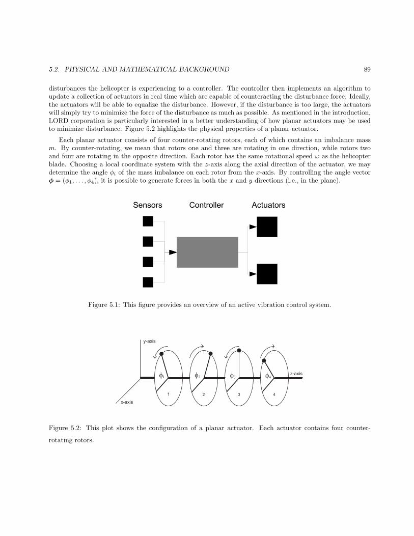
5.2. PHYSICAL AND MATHEMATICAL BACKGROUND 89
disturbances the helicopter is experiencing to a controller. The controller then implements an algorithm toupdate a collection of actuators in real time which are capable of counteracting the disturbance force. Ideally,the actuators will be able to equalize the disturbance. However, if the disturbance is too large, the actuatorswill simply try to minimize the force of the disturbance as much as possible. As mentioned in the introduction,LORD corporation is particularly interested in a better understanding of how planar actuators may be usedto minimize disturbance. Figure 5.2 highlights the physical properties of a planar actuator.
Each planar actuator consists of four counter-rotating rotors, each of which contains an imbalance massm. By counter-rotating, we mean that rotors one and three are rotating in one direction, while rotors twoand four are rotating in the opposite direction. Each rotor has the same rotational speed ω as the helicopterblade. Choosing a local coordinate system with the z-axis along the axial direction of the actuator, we maydetermine the angle φi of the mass imbalance on each rotor from the x-axis. By controlling the angle vectorφ = (φ1, . . . , φ4), it is possible to generate forces in both the x and y directions (i.e., in the plane).
Figure 5.1: This figure provides an overview of an active vibration control system.
x-axis
y-axis
z-axis
1 2 3 4
Figure 5.2: This plot shows the configuration of a planar actuator. Each actuator contains four counter-
rotating rotors.

90 CHAPTER 5. PROPERTIES OF A GRADIENT DESCENT ALGORITHM
5.2.1 Mathematical Formulation of the Active Vibration Control System
Consider the case of n sensors and m planar actuators, where there are more sensors than planar actuators,i.e., n ≥ 2m. The planar force vector F generated by each planar actuator, at frequency ω and time t, hascomponents
Fx(t) = ρ
4∑
j=1
cos((−1)jωt+ φj) (5.1)
Fy(t) = ρ
4∑
j=1
sin((−1)jωt+ φj) (5.2)
where ρ = mbω2, and mb is the rotator imbalance in units of kg·m. By applying the Fourier transform, wemay switch to the frequency domain and express Equations 5.1 and 5.2 in terms of cos(ωt) and sin(ωt) as
Fx = ρ4∑
j=1
[cos(φj) + i(−1)j sin(φj)
](5.3)
Fy = ρ
4∑
j=1
[sin(φj) + i(−1)j−1 cos(φj)
]. (5.4)
Note that the components Fx and Fy, resulting from the Fourier transform, are usually complex numbers.
Generalizing to the case of m actuators, we may express the total counteracting force produced by theplanar actuators as a vector:
u(φ)2m×1 = ρΨΦ (5.5)
where
Φ8m×1 =
cos(φ1,1)sin(φ1,1)cos(φ1,2)sin(φ1,2)
...cos(φm,4)sin(φm,4)
, (5.6)
φ4m×1 = φj,kj=1...m,k=1...4 denotes the angles of the 4m mass balances, and Ψ2m×8m is a block diagonalmatrix of the form
Ψ2m×8m =
ψ2×8 0 . . . 0
0 ψ2×8
......
. . . 00 . . . 0 ψ2×8
(5.7)
with diagonal blocks
ψ2×8 =
(1 −i 1 i 1 −i 1 ii 1 −i 1 i 1 −i 1
). (5.8)

5.2. PHYSICAL AND MATHEMATICAL BACKGROUND 91
We may then model our general system by the equation
e = d + Cu(φ) (5.9)
where dn×1 denotes the disturbance returned from the sensors, Cn×2m denotes the transfer matrix at ω betweenthe controls φ and e, and en×1 measures the difference between the disturbance and the counteracting forceof the planar actuators. The goal of our algorithm is to minimize the cost function
J(φ) = e(φ)∗e(φ). (5.10)
Furthermore, we demonstrate that the cost function J has a unique minimum in the following theorem.
Theorem 5.2.1. The cost function J defined in Equation 5.10 has a global minimum at some point φmin
Proof. The domain of the cost function J is periodic because e is a periodic function of φ. Without loss
of generality, we can choose this domain to be closed by restricting each component of φ to be in the set
φi : 0 ≤ φi ≤ 2π. Furthermore, J is continuous and bounded below by zero. Because J is a bounded
continuous function on a closed and bounded set, it has a global minimum at some point φmin in the domain
of φ.
However, because J is non-quadratic in φ, finding an analytical expression for φmin is a non-trivial task.Therefore, we employ numerical algorithms to find a numerical approximation of the minimum. As thealgorithms used to minimize the cost function will employ descent methods, they require the gradient of J ,denoted by ∇J , which is derived in Appendix B. In full vector notation, the gradient can be written as
∇J = 2ρRe
(∂Φ⊤
∂φΨ∗C∗e
)(5.11)
where
(∂Φ⊤
∂φ
)
4m×8m
=
− sin(φ1,1) cos(φ1,1) 0 0 · · ·0 0 − sin(φ1,2) cos(φ1,2)...
.... . .
. . .
0 0 − sin(φm,4) cos(φm,4)
,
(5.12)where, in addition to the derivation in Appendix B, we have made use of the formula
∂u∗
∂φ=∂Φ⊤
∂φΨ∗. (5.13)
5.2.2 A Comparison of Linear Actuators and Planar Actuators
In the section above, we discussed planar actuators. It is worthwhile to compare the latter to those currentlyused by LORD Corporation, which are linear actuators that generate force in a single direction. Whereasplanar actuators generate force in two directions. A comparison of the the two actuators will illustrate some

92 CHAPTER 5. PROPERTIES OF A GRADIENT DESCENT ALGORITHM
of the dynamic properties of the planar actuator and difficulties in minimizing the cost function defined inEquation 5.10.
For the case of the linear actuators, the system is modeled by the equation
e = d + Cu (5.14)
where u2m×1 is the control parameter denoting the force of the linear actuator, and dn×1 and Cn×2m representthe disturbance and transfer matrix as before. The system is linear with respect to the control parameter u.Moreover, the cost function
J(u) = e(u)∗e(u)
= d∗d + u∗C∗Cu + u∗C∗d + d∗Cu(5.15)
is quadratic in u and positive definite. Therefore J(u) has a unique minimum. The optimal choice of u, i.e.the one which yields the minimum of J , is the well-known solution to the least-squares problem:
uopt = −(C∗C)−1C∗d. (5.16)
A significant difference between the linear actuator and the planar actuator comes from an analysis of thefollowing two sets
U = C2m (5.17)
Φ = φj,k : 0 ≤ φj,k < 2π, j = 1, . . . , 2m, k = 1, . . . , 4. (5.18)
Clearly, u(φ) : φ ∈ Φ is strictly contained in U . Here, u(φ) is defined by Equation 5.5. In practice, linearactuators may not recognize uopt. If there exists φopt ∈ Φ such that u(φopt) = uopt, then clearly the choiceof φopt is the optimal choice for minimizing the cost function J(φ). However, it is not clear under whatcircumstances such a φopt exists. When it does not exist, the force from the optimal configuration of linearactuators does not match that from the optimal configuration of the planar actuators.
A second and more significant difference between the two actuators is that for planar actuators e(φ) is notlinear in the control parameter. Thus, J(φ) is not quadratic in φ. In this scenario, we cannot guarantee thatthe only critical points are at the unique minimum. For example, local minimum or saddle points may occurfor some values of φ. In these cases, numerical algorithms to minimize J(φ) may not converge to the globalminimum.
5.2.3 Saturation
When the magnitude of the disturbance force d becomes too large for the planar actuators to equalize, aninteresting physical and mathematical phenomenon called saturation occurs. In the case of saturation theplanar actuators generate maximum force in one or more directions. Physically, during saturation, pairs ofrotators rotating in the same direction align to the same angle. Mathematically, for the case of a singleactuator, this translates into φ1 = φ3 or φ2 = φ4. If both φ1 = φ3 and φ2 = φ4 we say that the actuator isfully saturated.
Under scenarios where one expects full saturation (i.e. the magnitude of d is large) we may reduce thecost function for a single actuator from four variables to two. This allows significant insight into our problem,as we can plot the cost function as a three dimensional surface. Figure 5.3 contains four contour plots ofthe cost function J(φ1 = φ3, φ2 = φ4) for four randomly generated disturbances d3×1 and respective transfermatrices C3×2. Each component of the disturbance vector d was randomly selected with a zero-mean Gaussian

5.2. PHYSICAL AND MATHEMATICAL BACKGROUND 93
distribution with standard deviation 8. Similarly, the entries of the transfer matrix C were randomly selectedfrom a zero-mean Gaussian distribution with unit standard deviation.
Darker areas represent lower values of the cost function J(φ), while lighter areas represent larger valuesJ(φ). We also note that these plots are periodic in φ1 and φ2 with period 2π because J(φ) is periodic in φ.Two observations are clear from Figure 5.3. First, when the actuator is fully saturated there exists a uniqueminimum and a unique maximum. No local minimum exists. Second, there exist saddle points, i.e. placeswhere the Hessian HJ(φ) has negative eigenvalues. Based on this we offer the following conjecture.
0 1 2 3 4 5 60
1
2
3
4
5
6
JHΦ1,Φ2L
0 1 2 3 4 5 60
1
2
3
4
5
6
JHΦ1,Φ2L
0 1 2 3 4 5 60
1
2
3
4
5
6
JHΦ1,Φ2L
0 1 2 3 4 5 60
1
2
3
4
5
6
JHΦ1,Φ2L
Figure 5.3: Contour Plots of the Cost Function J(φ1 = φ3, φ2 = φ4) For the Case of One Actuator Fully
Saturated
Conjecture 5.2.2. For the case of a fully saturated single actuator, there exists a φopt such that J(φopt) <
J(φ) for all φ 6= φopt. Moreover, any φ 6= φopt satisfying ∇J(φ) = 0 is either a saddle point or the global
maximum.
Numerical investigations of saturation for the case of multiple planar actuators are discussed in Section5.4.

94 CHAPTER 5. PROPERTIES OF A GRADIENT DESCENT ALGORITHM
5.3 Numerical Algorithms
Our optimization problem is defined as follows:
Find φopt such that J(φopt) = minφJ(φ), (5.19)
where no constraints are placed on the 4m×1 real vector φ. Moreover, recall that the cost function J , definedby Equation 5.10 in the previous section, is nonlinear and non-quadratic in φ.
Most numerical algorithms used to minimize (or maximize) a function in the absence of any constraintsproceed by finding a direction along which the cost function decreases (or increases). Then, a step size isminimized (or maximized) along this direction. Therefore, descent algorithms can be decomposed into threedistinct steps:
1. Compute a search direction along which the cost function decreases or increases.
2. Find the optimal step size, and take a step in the search direction.
3. Update the state variable and any supporting quantities.
For our numerical experiments, we modified C. T. Kelley’s implementation6 of the algorithms discussed inhis book [5]. We focused primarily on the steepest (or gradient) descent method and the Broyden–Fletcher–Goldfarb–Shanno (BFGS) quasi-Newton method. In each case, the goal was to minimize the nonlinear costfunction J(φ) given in Equation 5.10. A MATLAB script implementing the BFGS algorithm is included inAppendix A.
5.3.1 The Method of Steepest Descent
The method of steepest descent is one of the most common algorithms for minimizing (or maximizing) adifferentiable function of several variables. Recall that a vector p is a direction of descent of a function J atφ if there is a δ > 0 such that J(φ + µp) < J(φ) for all µ ∈ (0, δ). The method of steepest descent movesalong a direction p such that ‖p‖2 = 1. If the function J is differentiable at φ with a nonzero gradient, thenp = −∇J(φ)/‖∇J(φ)‖2 is the direction of steepest descent.
The steepest descent algorithm for our minimization problem given in Equation 5.19 is summarized asfollows:
1. Chose an initial guess for our solution, φ0.
2. Compute the gradient of the cost function J , ∇J(φk). If the gradient is small, terminate the process.Otherwise, we let the steepest descent direction be pk = −∇J(φk) and compute the iterates as:
φk+1 = φk − µkpk, k ≥ 0 (5.20)
where k is the iteration, pk is the descent direction and µk is the step-size parameter.
If J is quadratic in φ, we can derive constraints on the step size µ in terms of the singular values of theJacobian of J . Unfortunately, since J is not quadratic in φ, we cannot derive the usual restriction on µ.
6The MATLAB scripts are freely available online at http://www4.ncsu.edu/~ctk/matlab darts.html.

5.3. NUMERICAL ALGORITHMS 95
Therefore, we have two options: pick µk = µ ≪ 1, ∀k and hope the iterates computed via Equation 5.20converge, or use a line search to find the best µk for each step k.
Steepest descent usually reduces the cost function dramatically during the early stages of the optimizationprocess, depending on the point of initialization. However, the method usually behaves poorly near thestationary point, taking small, nearly orthogonal steps. Zigzagging and poor convergence for the steepestdescent algorithm can be overcome by deflecting the gradient. That is, instead of moving along the directionp = −∇J(φ), we can move along p = −P∇J(φ) or along p = −P∇J(φ) + v, for some positive definitematrix P and vector v.
Though simple, steepest descent’s convergence is typically slow even in the best case scenarios [7]. Conse-quently, we must consider a better minimization algorithm.
5.3.2 Newton’s Method
Newton’s method is very similar to steepest descent, except that, at each iteration, the search direction isdeflected by premultiplying it by the inverse of the Hessian matrix. The latter is essentially a correction to thesearch direction via a local, quadratic approximation to the cost function. Consequently, the iteration schemefor this algorithm is:
1. Chose a good initial guess, φ0 for the solution.
2. Update the state variable via the iteration scheme φk+1 = φk − [HJ(φk)]−1∇J(φk), k ≥ 0,
where recall that HJ(·) denotes the Hessian of J . As in the previous algorithm, the iteration continues untila suitable termination criterion is met. The main advantage of Newton’s method is that it converges rapidlywhen the initial guess is close to the solution. A disadvantage of this method is that it requires the calculationof the Hessian matrix at each step. Furthermore, it has poor convergence properties if the Hessian at theminimum is positive semidefinite [7].
5.3.3 The BFGS Quasi-Newton Method
Yet another class of widely-used algorithms for nonlinear optimization are the quasi-Newton methods. UnlikeNewton’s method, the latter approximate either the Hessian HJ or its inverse [HJ ]−1, at each iteration, witha matrix that is available at lower cost. In what follows, the approximation to the Hessian is representedby Bk, and the approximation to the Hessian’s inverse is represented by Ck. Quasi-Newton methods thenuse these approximations to compute an approximation to the search direction of Newton’s method, i.e.[HJ(φk)]−1∇J(φk) ≈ B−1
k ∇J(φk) or [HJ(φk)]−1∇J(φk) ≈ Ck∇J(φk).The Broyden–Fletcher–Goldfarb–Shanno (BFGS) method is a particular quasi-Newton method that ap-
proximates the Hessian at each step. The algorithm requires an initial guess for the minimum, φ0, and aninitial positive definite approximation to the Hessian of J , which we denote by B0. Typically, a suitable initialapproximation to the Hessian is the identity matrix, B0 = I (see, e.g., [5, 7]). Then, the BFGS method canbe implemented via the following iteration scheme:
1. Compute a search direction: pk = B−1k ∇J(φk).
2. Use a line search to find an optimal step size µk in the direction of pk.
3. Update the state variable: φk+1 = φk − µkpk.

96 CHAPTER 5. PROPERTIES OF A GRADIENT DESCENT ALGORITHM
4. Update the approximation of the Hessian: Bk+1 = Bk +yky⊤
k
y⊤
ksk
− (Bksk)(Bksk)⊤
s⊤k
Bksk, where yk = ∇J(φk+1)−
∇J(φk) and sk = φk+1 − φk.
The iteration is terminated when ‖∇J(φk)‖2 ≤ ǫ for some ǫ≪ 1.
It can be shown that if Bk is a symmetric positive definite matrix, then Bk+1 is positive definite if andonly if y⊤
k sk > 0 [2, 6]. Performing an appropriate line search can guarantee this condition. If this conditionis met, then BFGS typically has stable convergence properties [7].
Alternately, we could have used a quasi-Newton method like the Davidson–Fletcher–Powell (DFP) one,which approximates the inverse of the Hessian at each iteration. These algorithms avoid the costly inversionof the approximate Hessian. However, though computationally cheaper, these methods can have troubleconverging if the true Hessian at the minimum is singular [7]. Thus, before implementing a method like DFPfor the active vibration control problem, we would need more knowledge of the properties of the Hessian atthe minimum. Furthermore, numerous convergence experiments would have to be run to ensure the stabilityof the DFP algorithm, especially in cases like saturation. Therefore, we believe that BFGS is superior to DFPfor the purposes of our problem.
In addition, it should be noted that the version of the BFGS algorithm that C. T. Kelley implements inhis MATLAB scripts is a different one from the algorithm formulated in his book [5]. Instead of updating Bk
at each iteration, the search direction pk = B−1k ∇J(φk) is updated directly. By doing so, one avoids having
to store the (possibly large) matrix Bk at each step. Finally, the search direction is also modified, thoughslightly, to guarantee that the function being minimized decreases at each step.
5.3.4 Convergence of Descent Methods
The numerical experiments presented in the next section suggest that the steepest descent and BFGS methodsconverge to a local minimum of the cost function J . We wish to demonstrate that they will always convergeto that local minimum. Both steepest descent and BFGS are in a larger class of minimization schemes, knownas descent methods. The convergence of descent methods to fixed points has been well established [2, 5, 6].
Both BFGS and steepest descent are descent methods for minimization. That is, for both these methodsφk+1 = φk − µkpk, where −pk is in a “downhill” direction from the point φk, i.e. it is such that
−p⊤k ∇J(φk) < 0. (5.21)
For the steepest descent method, we choose −pk = −∇J(φk). Therefore, the descent condition in Equa-tion 5.21 is satisfied by construction. For the BFGS method, we choose −pk = −B−1
k ∇J(φk). Bk is definedabove, and by construction is symmetric positive definite at each step k [2]. Therefore, B−1
k is also symmetricpositive definite. By the definition of positive definite matrices, the descent condition in Equation 5.21 issatisfied.
Fletcher [2] proves the global convergence of descent methods under certain conditions.
Theorem 5.3.1 (Global convergence of descent methods). For a descent method with step µk satisfying the
Wolfe–Powell conditions and pk satisfying orthogonality conditions, if ∇J exists and is uniformly continuous
on the level set φ : J(φ) < J(φ0) , and if J is bounded from below, then either ∇J(φk) = 0 or ∇J(φk) → 0.

5.3. NUMERICAL ALGORITHMS 97
Here, the Wolfe–Powell conditions are satisfied when the step µk is a parameter for which
J(φk − µkpk) ≤ J(φk) − σαµk∇J(φk)⊤pk, (5.22)
and∇J(φk − µkpk)⊤pk ≥ σβ∇− J(φk)⊤pk, (5.23)
where 0 < σα < σβ < 1/2. The orthogonality conditions on pk are satisfied when
∇J(φk)⊤pk
‖∇J(φk)‖2 ‖pk‖2
≥ ǫ, (5.24)
for some ǫ > 0.Using Theorem 5.3.1, we can demonstrate that the cost function J we are minimizing in this problem will
converge to a fixed point.
Theorem 5.3.2. Descent methods with a line search will converge to a fixed point of the cost function J
defined in Equation 5.10.
Proof. The cost function J we are minimizing in this problem is smooth and bounded below by zero. Therefore,
it satisfies the conditions of Theorem 5.3.1. If we use a line search to choose µk in the steepest descent method
or the BFGS method, the Wolfe–Powell conditions are satisfied automatically. Furthermore, based on the
discussion above, which shows that BFGS and steepest descent are part of the class of so-called descent
algorithms, we expect that the orthogonality conditions are met for these two methods. We have argued that
all the conditions of Theorem 5.3.1 are met. Therefore, we conclude that in this case the descent methods will
converge to a fixed point of J .
We also observe convergence for fixed step µk = µ in steepest descent. Therefore, we conjecture that itwill converge in this case.
Conjecture 5.3.3. A descent method with a fixed step µ that satisfies appropriate bounds will converge to a
fixed point of the cost function J defined in Equation 5.10.
Finding bounds which ensure that the fixed step µ satisfies the Wolfe–Powell and orthogonality conditionswould verify this conjecture.
It is important to note that Theorem 5.3.1 only guarantees that the descent algorithms will converge to afixed point. There is no guarantee that this fixed point will be a minimum. Nonetheless, Fletcher [2] claimsthat typically the descent methods will converge to a local minimum because the line search reduces the valueof J at each step. Furthermore, because we are observing convergence for a fixed step µ, we also expect thedescent algorithm to converge to a local minimum in this case.
Conjecture 5.3.4. With probability one, a descent method with an appropriate step size µk will converge to
a local minimum φmin of the cost function J defined in Equation 5.10.

98 CHAPTER 5. PROPERTIES OF A GRADIENT DESCENT ALGORITHM
This convergence to a local minimum can be demonstrated if the Hessian of J is symmetric positive definite(see, e.g., [5]). Furthermore, the convergence of BFGS will be superlinear if the Hessian of J is symmetricpositive definite at the fixed point. We therefore explore the behavior of the Hessian in the next section.
5.3.5 The Hessian
To ensure that the algorithm converges to a true minimum and not a saddle point, we would like to show theHessian is positive definite at every numerically computed minimum φmin. In order to make the computationof the analytical Hessian feasible, we made the simplifying assumption that the system consists of one actuator,two sensors, and we have C = 1/m. Note that C is assumed to be a real scalar, not a complex matrix. We letFx = Fx1
+ iFx2and Fy = Fy1
+ iFy2. Then we have
J(φ) =1
m2
(8 + |Fx|2 + |Fy |2 + 4 cos (φ1 − φ3) + 4 cos (φ2 − φ4)
+ 2Fx1
∑
i
cos (φi) + 2Fy1
∑
i
sin (φi) + 2Fy2
∑
i
(−1)i cos (φi)
+ 2Fx2
∑
i
(−1)i−1 sin (φi)).
(5.25)
We can also explicitly compute ∇J(φ) as
∇J(φ) =2
m2
2 sin (φ3 − φ1) − Fx1sin (φ1) + Fy1
cos (φ1) + Fy2sin (φ1) + Fx2
cos (φ1)2 sin (φ4 − φ2) − Fx1
sin (φ2) + Fy1cos (φ2) − Fy2
sin (φ2) − Fx2cos (φ2)
2 sin (φ1 − φ3) − Fx1sin (φ3) + Fy1
cos (φ3) + Fy2sin (φ3) + Fx2
cos (φ3)2 sin (φ4 − φ2) − Fx1
sin (φ4) + Fy1cos (φ4) − Fy2
sin (φ4) − Fx2cos (φ4)
. (5.26)
From the latter we can compute the components of the Hessian, which is the matrix
HJ =
HJ11 HJ12 HJ13 HJ14
HJ21 HJ22 HJ23 HJ24
HJ31 HJ32 HJ33 HJ34
HJ41 HJ42 HJ43 HJ44
, (5.27)

5.3. NUMERICAL ALGORITHMS 99
and its only nonzero entries are
HJ11 =2
m2[−2 cos(φ1 − φ3) + Fy2
cos(φ1) − Fx2sin(φ1) − Fx1
cos(φ1) − Fy1sin(φ1)] ,
HJ13 =4
m2cos(φ1 − φ3),
HJ22 =2
m2[−2 cos(φ2 − φ4) − Fy2
cos(φ2) + Fx2sin(φ2) − Fx1
cos(φ2) − Fy1sin(φ2)] ,
HJ24 =4
m2cos(φ2 − φ4),
HJ31 =4
m2cos(φ1 − φ3),
HJ33 =2
m2[−2 cos(φ1 − φ3) + Fy2
cos(φ3) − Fx2sin(φ3) − Fx1
cos(φ3) − Fy1sin(φ3)] ,
HJ42 =4
m2cos(φ2 − φ4),
HJ44 =2
m2[−2 cos(φ2 − φ4) − Fy2
cos(φ4) + Fx2sin(φ4) − Fx1
cos(φ4) − Fy1sin(φ4)] .
(5.28)
Conjecture 5.3.5. Given J(φ) as above, the Hessian HJ is positive definite at every minimum φmin where
the descent algorithms converge to φmin.
In order to prove this, we would need to show that HJ (φmin) has strictly positive eigenvalues. Numericalexperiments on the system with the Hessian in Equation 5.28 lead us to believe that this conjecture is cor-rect. Note that this condition only guarantees that the proposed solution converges to a local minimum, notnecessarily a global minimum.
5.3.6 Decreasing the Step-Size to Satisfy Angular Constraints
In practice, the planar actuator adjusts its configuration to match the angles suggested by the numericalalgorithm at each iteration. Therefore, it is desirable that none of the angles change “too quickly” betweeniterations. That is, we would like ‖∆φk+1‖∞ ≡ ‖φk+1 −φk‖∞ to be bounded above by some constant ∆φmax
at each step.To this end, we have developed an algorithm to constrain the step size µk. Regardless of the numerical
minimization scheme, φk+1 = φk − µkpk. Therefore, ∆φk+1 = −µkpk and ‖∆φk+1‖∞ = µk‖pk‖∞. If,for some k, we have that µk > ∆φmax/‖pk‖∞, then set µk = ∆φmax/‖pk‖∞. This restriction will ensurethat ‖∆φk+1‖∞ = ∆φmax. If we wish to avoid the cost associated with implementing a line search, we canuse µk = ∆φmax/‖pk‖∞ for each iteration. In this case, ∆φmax should be small enough to ensure that theminimization algorithm will converge.
Whether we use µk with a line search and then constrain it as above or use the constrained µk directly,we observe convergence for both the BFGS and steepest descent. We therefore conjecture that these descentschemes converge for these µk’s.
Conjecture 5.3.6. A descent method using the constrained µk with or without a line search will converge to
a fixed point of the cost function J in Equation 5.10.

100 CHAPTER 5. PROPERTIES OF A GRADIENT DESCENT ALGORITHM
Again, we could verify this conjecture by showing that these constrained µk’s satisfy the Wolfe–Powellconditions in Equations 5.23 and 5.24. For BFGS, we would also have to demonstrate that for this choice ofµk the approximation to the Hessian Bk remains positive definite at each step.
Furthermore, the above fix is roughly equivalent to solving a weakly-constrained optimization problem,which penalizes large changes in the rotor angles. For this case, instead of minimizing the original (uncon-strained) problem of minimizing J , we minimize the following modified cost function
J = e∗e + α‖∆φk+1‖2∞. (5.29)
Here, we would tune α to give an appropriate penalty for large changes in the angle. Recall, ∆φk+1 = −µkpk.Therefore,
J = e∗e + αµ2k‖pk‖2
∞. (5.30)
In implementing the above restrictions on µk, we decrease µk but keep pk fixed. In this case, the algorithm ismoving in a descent direction at each step and the e∗e term of J decreases. The second term also decreasesbecause µk decreases. Therefore, we expect that limiting µk is similar to minimizing J .
In practice, constraining the step size during the steepest descent and BFGS schemes prevents the actuatorfrom changing too dramatically, but increases the number of iterations needed to reach convergence. Further-more, we observe little difference in convergence for using the constrained µk with and without a line search.Therefore, for the numerical experiments below we use the constrained µk without a line search.
5.3.7 Global Minimization Algorithms
To support our conjecture that the above numerical methods are converging to a global minimum, we comparedour solutions to those given by the DIRECT algorithm7 developed in [8, 3].
It should be noted that the stopping criterion that DIRECT most often reaches is not the one that guaranteesa minimum but one on the number of cost function evaluations. Therefore, as expected, the latter is not acompetitive method but it provides a good way to benchmark the BFGS and steepest descent methods.
5.4 Numerical Results
To evaluate the performance of the optimization algorithms described in Section 5.3, we performed numericalexperiments for various combinations of the free parameters (i.e., m, n, ρ, C, d). In this section, we presentsome illustrative numerical simulations for m = 2, n = 5, ρ = 1, and random C and d chosen from a zero-meanGaussian distribution. If the algorithms perform well for a wide range of random C and d, then we can expectthem to perform well in real physical situations.
Furthermore, in the discussion below, the components of a “small disturbance” are chosen with a standarddeviation of 1, while the components of a “large disturbance” are chosen with a standard deviation of 50. Thestandard deviation for the large disturbance case was chosen to be 50 because this value typically leads to fullsaturation. Finally, for all simulations in this section, we used ∆φmax = π/16, and the initial guess for theangles of each actuator is always φj = φ2j = 0, φ3j = φ4j = π, j = 1, . . . ,m.
7We used Daniel Finkel’s implementation of DIRECT available freely online at http://www4.ncsu.edu/~ctk/Finkel Direct/.
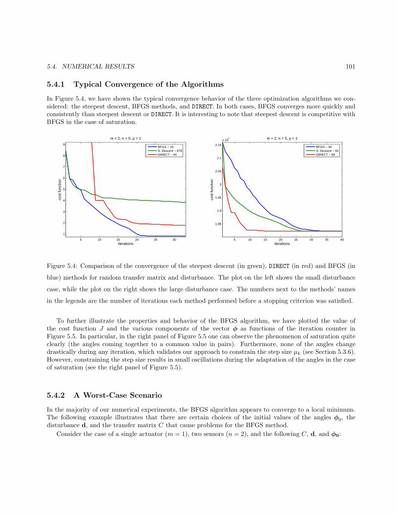
5.4. NUMERICAL RESULTS 101
5.4.1 Typical Convergence of the Algorithms
In Figure 5.4, we have shown the typical convergence behavior of the three optimization algorithms we con-sidered: the steepest descent, BFGS methods, and DIRECT. In both cases, BFGS converges more quickly andconsistently than steepest descent or DIRECT. It is interesting to note that steepest descent is competitive withBFGS in the case of saturation.
5 10 15 20 25 30
1
2
3
4
5
6
7
8
9
iterations
cost
func
tion
m = 2, n = 5, ρ = 1
BFGS − 33S. Descent − 676DIRECT − 44
5 10 15 20 25 30 35 40
1.85
1.9
1.95
2
2.05
2.1
2.15
x 104
iterations
cost
func
tion
m = 2, n = 5, ρ = 1
BFGS − 40S. Descent − 92DIRECT − 68
Figure 5.4: Comparison of the convergence of the steepest descent (in green), DIRECT (in red) and BFGS (in
blue) methods for random transfer matrix and disturbance. The plot on the left shows the small disturbance
case, while the plot on the right shows the large disturbance case. The numbers next to the methods’ names
in the legends are the number of iterations each method performed before a stopping criterion was satisfied.
To further illustrate the properties and behavior of the BFGS algorithm, we have plotted the value ofthe cost function J and the various components of the vector φ as functions of the iteration counter inFigure 5.5. In particular, in the right panel of Figure 5.5 one can observe the phenomenon of saturation quiteclearly (the angles coming together to a common value in pairs). Furthermore, none of the angles changedrastically during any iteration, which validates our approach to constrain the step size µk (see Section 5.3.6).However, constraining the step size results in small oscillations during the adaptation of the angles in the caseof saturation (see the right panel of Figure 5.5).
5.4.2 A Worst-Case Scenario
In the majority of our numerical experiments, the BFGS algorithm appears to converge to a local minimum.The following example illustrates that there are certain choices of the initial values of the angles φ0, thedisturbance d, and the transfer matrix C that cause problems for the BFGS method.
Consider the case of a single actuator (m = 1), two sensors (n = 2), and the following C, d, and φ0:

102 CHAPTER 5. PROPERTIES OF A GRADIENT DESCENT ALGORITHM
5 10 15 20 25
2
3
4
5
6
7
iterations
m = 2, n = 5, ρ = 1
J
|d|
5 10 15 20 25
−1
0
1
2
3
4
iterations
angl
es
5 10 15 20 25 30 35 40
3.5
3.6
3.7
3.8
3.9
4
4.1x 10
4
iterations
m = 2, n = 5, ρ = 1
J
|d|
5 10 15 20 25 30 35 40
0
1
2
3
iterations
angl
esFigure 5.5: Convergence to a minimum and adaptation of the angles via the BFGS method. The plot on
the left shows the small disturbance case, while the plot on the right shows the large disturbance case and
saturation.
C =
0.5508 + i0.1986 0.79241 + i0.67201.2037 + i0.2488 1.21074 + i0.24782.0377 + i0.5197 0.29025 + i0.0998
, d =
−0.0775− i0.0237+1.9558− i1.3703−0.3048 + i0.1139
, φ0 =
5551
. (5.31)
The initial conditions indicate that rotors one and three are saturated. Using these initial conditions, applyingthe BFGS algorithm yields a minimum of 12.06285. However, perturbing the initial conditions only slightly,i.e. taking
φ0′ =
55
5.011
, (5.32)
yields a minimum of 2.82096, which appears to be the global minimum as computed by DIRECT. We believethe issue is not related to the existence of local minima but rather a factor of precision. To support the latteridea, we used Mathematica to run the BFGS algorithm using a precision of 10−75, which is a lot more thanMATLAB’s double precision (10−16), and obtained a minimum of 2.82096. It should be noted that this worstcase scenario was found by trying to break the proposed algorithm. In practice, the initial conditions arealmost as arbitrary as randomly generated ones, thus we do not believe such worst-case scenarios would be anissue. Nevertheless, we cite it as a possibility.
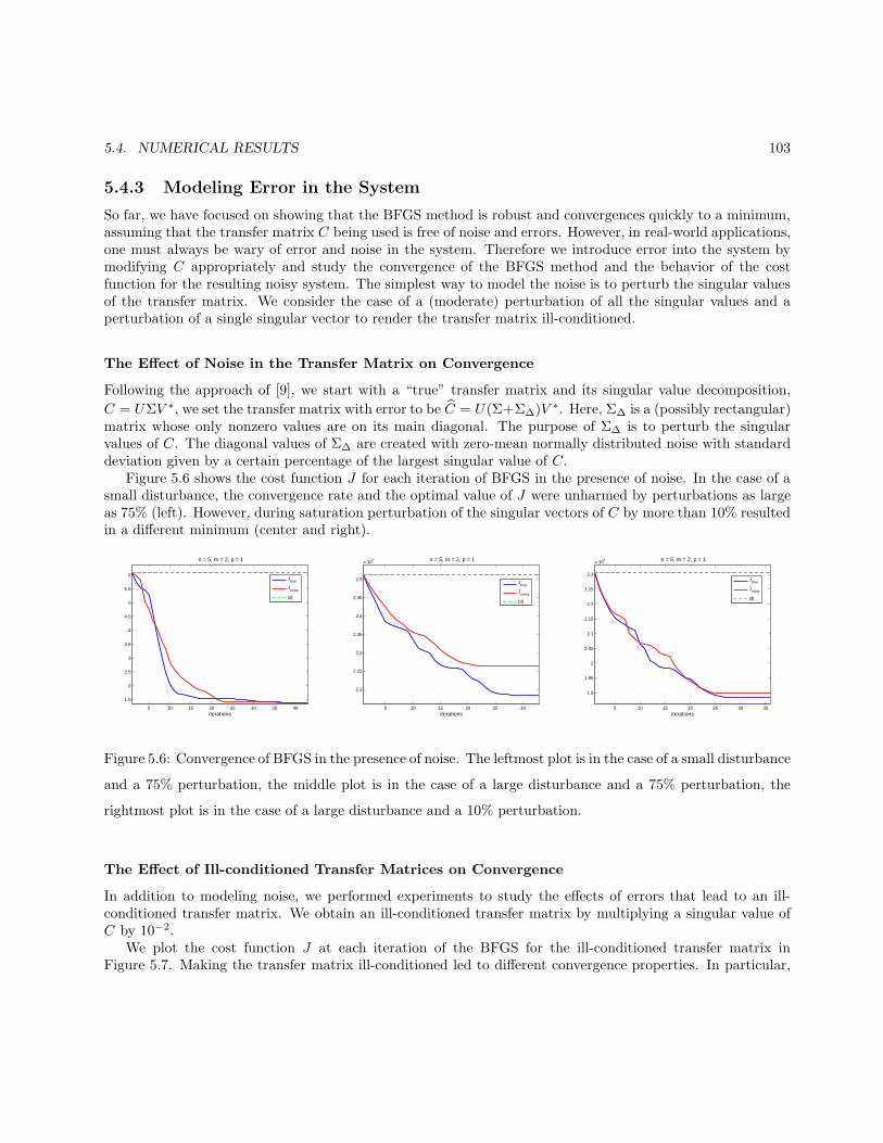
5.4. NUMERICAL RESULTS 103
5.4.3 Modeling Error in the System
So far, we have focused on showing that the BFGS method is robust and convergences quickly to a minimum,assuming that the transfer matrix C being used is free of noise and errors. However, in real-world applications,one must always be wary of error and noise in the system. Therefore we introduce error into the system bymodifying C appropriately and study the convergence of the BFGS method and the behavior of the costfunction for the resulting noisy system. The simplest way to model the noise is to perturb the singular valuesof the transfer matrix. We consider the case of a (moderate) perturbation of all the singular values and aperturbation of a single singular vector to render the transfer matrix ill-conditioned.
The Effect of Noise in the Transfer Matrix on Convergence
Following the approach of [9], we start with a “true” transfer matrix and its singular value decomposition,
C = UΣV ∗, we set the transfer matrix with error to be C = U(Σ+Σ∆)V ∗. Here, Σ∆ is a (possibly rectangular)matrix whose only nonzero values are on its main diagonal. The purpose of Σ∆ is to perturb the singularvalues of C. The diagonal values of Σ∆ are created with zero-mean normally distributed noise with standarddeviation given by a certain percentage of the largest singular value of C.
Figure 5.6 shows the cost function J for each iteration of BFGS in the presence of noise. In the case of asmall disturbance, the convergence rate and the optimal value of J were unharmed by perturbations as largeas 75% (left). However, during saturation perturbation of the singular vectors of C by more than 10% resultedin a different minimum (center and right).
5 10 15 20 25 30 35 40
1.5
2
2.5
3
3.5
4
4.5
5
5.5
6
iterations
n = 5, m = 2, ρ = 1
Jtrue
Jnoisy
|d|
5 10 15 20 25 30
2.2
2.25
2.3
2.35
2.4
2.45
2.5
x 104
iterations
n = 5, m = 2, ρ = 1
Jtrue
Jnoisy
|d|
5 10 15 20 25 30 35
1.9
1.95
2
2.05
2.1
2.15
2.2
2.25
2.3
x 104
iterations
n = 5, m = 2, ρ = 1
Jtrue
Jnoisy
|d|
Figure 5.6: Convergence of BFGS in the presence of noise. The leftmost plot is in the case of a small disturbance
and a 75% perturbation, the middle plot is in the case of a large disturbance and a 75% perturbation, the
rightmost plot is in the case of a large disturbance and a 10% perturbation.
The Effect of Ill-conditioned Transfer Matrices on Convergence
In addition to modeling noise, we performed experiments to study the effects of errors that lead to an ill-conditioned transfer matrix. We obtain an ill-conditioned transfer matrix by multiplying a singular value ofC by 10−2.
We plot the cost function J at each iteration of the BFGS for the ill-conditioned transfer matrix inFigure 5.7. Making the transfer matrix ill-conditioned led to different convergence properties. In particular,

104 CHAPTER 5. PROPERTIES OF A GRADIENT DESCENT ALGORITHM
the minimization schemes converge to a different optimal value for both small and large disturbances. However,the efficiency and rate of convergence of the BFGS method were unaffected.
5 10 15 20 25
1
2
3
4
5
6
7
iterations
n = 5, m = 2, ρ = 1
Jtrue
Jperturbed
|d|
5 10 15 20 25 30
1.6
1.65
1.7
1.75
1.8
1.85
1.9
x 104
iterations
n = 5, m = 2, ρ = 1
Jtrue
Jperturbed
|d|
Figure 5.7: Comparison of the convergence to a minimum when a singular value of the transfer matrix is
perturbed so that C becomes ill conditioned; on the left is the case of a small disturbance, and on the right
is the case of a large disturbance.
5.4.4 Dependence of Jmin on n
Ideally, if the planar actuators are balancing the disturbance the cost function J would be zero. However, inmany cases we observe that the minimum of the cost function is significantly greater than zero. We observe thisparticularly when there are a large number of sensors. We perform several numerical experiments to elucidatethe dependence of the minimum of the cost function J on the number of sensors n. For these experiments,we solved 200 optimization problems (each with a random transfer matrix and initial disturbance) for eachn ≥ 2m (with m fixed), then averaged the minima of the cost function. In Figure 5.8, we have plotted theaverage minimum as a function of n. The figure suggests that Jmin ∼ const. ·n. In the small disturbance case,the constant has been experimentally determined to be 2. In general, we observe that the constant is of theform 2 × 10x, where x depends on the magnitude of the disturbance.
5.4.5 Adapting to a changing disturbance
In practice, the disturbance of the helicopter will change between iterations of the minimization algorithm.Whether these changes are gradual or sudden, the cost function must change at each step to reflect thenew disturbance. As a result, a minimization algorithm that takes dynamic disturbances into account mustimplement the following steps:
1. Compute a search direction along which the cost function decreases.
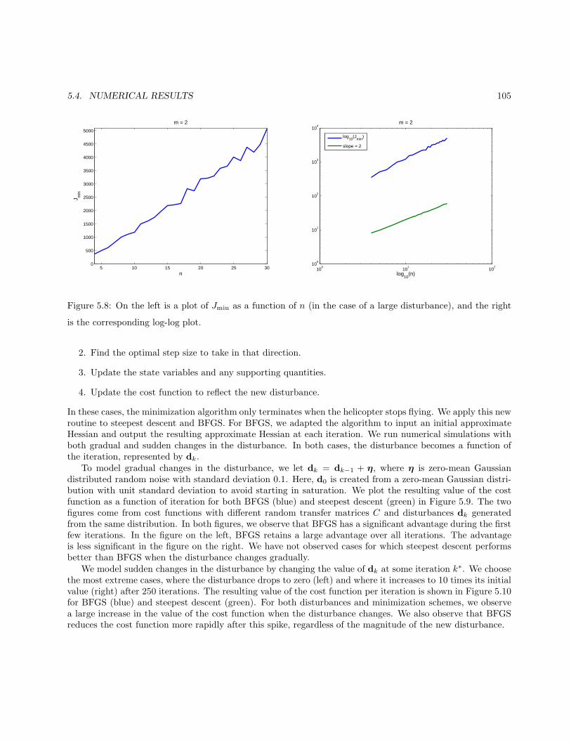
5.4. NUMERICAL RESULTS 105
5 10 15 20 25 300
500
1000
1500
2000
2500
3000
3500
4000
4500
5000
n
J min
m = 2
100
101
102
100
101
102
103
104
log10
(n)
m = 2
log10
(Jmin
)
slope = 2
Figure 5.8: On the left is a plot of Jmin as a function of n (in the case of a large disturbance), and the right
is the corresponding log-log plot.
2. Find the optimal step size to take in that direction.
3. Update the state variables and any supporting quantities.
4. Update the cost function to reflect the new disturbance.
In these cases, the minimization algorithm only terminates when the helicopter stops flying. We apply this newroutine to steepest descent and BFGS. For BFGS, we adapted the algorithm to input an initial approximateHessian and output the resulting approximate Hessian at each iteration. We run numerical simulations withboth gradual and sudden changes in the disturbance. In both cases, the disturbance becomes a function ofthe iteration, represented by dk.
To model gradual changes in the disturbance, we let dk = dk−1 + η, where η is zero-mean Gaussiandistributed random noise with standard deviation 0.1. Here, d0 is created from a zero-mean Gaussian distri-bution with unit standard deviation to avoid starting in saturation. We plot the resulting value of the costfunction as a function of iteration for both BFGS (blue) and steepest descent (green) in Figure 5.9. The twofigures come from cost functions with different random transfer matrices C and disturbances dk generatedfrom the same distribution. In both figures, we observe that BFGS has a significant advantage during the firstfew iterations. In the figure on the left, BFGS retains a large advantage over all iterations. The advantageis less significant in the figure on the right. We have not observed cases for which steepest descent performsbetter than BFGS when the disturbance changes gradually.
We model sudden changes in the disturbance by changing the value of dk at some iteration k∗. We choosethe most extreme cases, where the disturbance drops to zero (left) and where it increases to 10 times its initialvalue (right) after 250 iterations. The resulting value of the cost function per iteration is shown in Figure 5.10for BFGS (blue) and steepest descent (green). For both disturbances and minimization schemes, we observea large increase in the value of the cost function when the disturbance changes. We also observe that BFGSreduces the cost function more rapidly after this spike, regardless of the magnitude of the new disturbance.

106 CHAPTER 5. PROPERTIES OF A GRADIENT DESCENT ALGORITHM
0 50 100 150 200 250 300 350 400 450 5000
1
2
3
4
5
6
7
8
9
10
iterations
cost
func
tion
BFGSsteepest descent
0 50 100 150 200 250 300 350 400 450 5000
2
4
6
8
10
12
14
16
18
20
iterations
cost
func
tion
BFGSsteepest descent
Figure 5.9: This figure shows the value of the cost function at each iteration for BFGS (blue) and steepest
descent (green) when the disturbance changes gradually at each step. The two figures result from two different
choices of transfer matrix C and initial disturbance d0.
5.5 Conclusions
The numerical results presented in Section 5.4, suggest that the BFGS method converges to the minimum ofthe cost function defined in Equation 5.10 faster than the method of steepest descent, and is more robust (i.e.,performs well in a variety of different situations). In particular, the superiority of BFGS over steepest descentis most evident when the system is not saturated. In addition, our numerical experiments suggest that BFGSis converging to the minimum superlinearly, even though we cannot confirm analytically that that Hessian ofthe cost function at the minimum is positive definite. The proof of the latter warrants further work.
Furthermore, we found that the BFGS method is not affected by the presence of noise and/or error in thesystem. When the planar actuators are not saturated, the convergence properties of the BFGS method arepractically unchanged even for large perturbations of the singular values of the transfer matrix. In saturation,on the other hand, though the convergence of the BFGS method is still fast, the minimum found is unchangedonly for small perturbations of the singular values of the transfer matrix. Furthermore, BFGS convergesquickly to a minimum if the transfer matrix is ill-conditioned, regardless of the disturbance. However, thevalue of that minimum changes in this case.
In general, BFGS also converges more rapidly and accurately than steepest descent in the case of a dynamicdisturbance, i.e. when the magnitude of the disturbance changes at each iteration. The BFGS method’ssuperiority over steepest descent is most evident at the beginning of the iteration and immediately followinga dramatic change in the disturbance’s magnitude. If the disturbance changes gradually, the advantage ofBFGS over steepest descent may decrease later in the iteration. We suspect that BFGS is loosing its advantagebecause it is not modifying the approximate Hessian of the cost function appropriately in these later iterations.Further studies would need to be performed to verify this conjecture, and additional theoretical analysis wouldbe needed to determine the convergence properties of both BFGS and steepest descent in the case of a dynamicdisturbance.

5.5. CONCLUSIONS 107
0 50 100 150 200 250 300 350 400 450 5000
1
2
3
4
5
6
7
iterations
cost
func
tion
BFGSsteepest descent
0 50 100 150 200 250 300 350 400 450 5000
10
20
30
40
50
60
70
iterations
cost
func
tion
BFGSsteepest descent
Figure 5.10: This figure plots the value of the cost function at each iteration for BFGS (blue) and steepest
descent (green) when the disturbance changes suddenly at iteration 250. The disturbance drops to zero on
the left and to ten times its initial value on the right.
Furthermore, we found a particular choice of (randomly-generated) transfer matrix and disturbance thatresult in BFGS and steepest descent converging to an incorrect minimum. We suspect that the latter poorconvergence results are due to truncation error in the numerical computations. It should be noted, however,that we only observed the latter undesirable behavior when we tried to break the algorithm. Further theoreticalanalysis is needed to determine if this particular configuration (i.e., choice of transfer matrix and disturbance)can ever be realized physically.
Finally, recall that planar actuators cannot always balance the disturbance perfectly, i.e. the minimumof the cost function is not always zero. This is particularly evident when there is a large number of sensorsor the system is saturated. Future studies should examine bounds on the cost function as a function of thedisturbance. These bounds on the cost function would be particularly useful in determining whether saturationwill occur for a given disturbance.
Appendix A: MATLAB Scripts
Appendix A.1: The Driver Script — sim.m
clear all; close all;
m = 2; % # of actuators
n = 5; % # of sensors
rho = 1; % imbalance force

108 CHAPTER 5. PROPERTIES OF A GRADIENT DESCENT ALGORITHM
% generate random disturbance and transfer matrix
d = 1*(randn(n,1) + i*randn(n,1)); C = randn(n,2*m) + i*randn(n,2*m);
% generate psi
psi1 = [1 -i 1 i 1 -i 1 i; i 1 -i 1 i 1 -i 1]; psi = zeros(2*m,8*m);
for j = 1:m; psi(2*j-1:2*j,8*j-7:8*j) = psi1; end;
% initial conditions
dPdp = zeros(4*m,8*m); p1(:,1) = 1*[0 0 pi pi]’; p0 = []; for j = 1:m; p0 = [p0; p1]; end;
% CTK’s BFGS Quasi-Newton method (bfgswopt.m, polymod.m, polyline.m)
[phis,histout] = bfgswopt(p0, @(x) costfunc(x,m,rho,d,C,psi), ...
pi/16, 1.d-6, 1000);
iter = histout(:,4); Js = histout(:,2);
Appendix A.2: Our Modification of C. T. Kelley’s BFGS Solver — bfgswopt.m
function [xs,histout,costdata] =
bfgswopt(x0,f,dxmax,tol,maxit,hess0)
% C. T. Kelley, July 17, 1997
% Ivan Christov, modified on July 25, 2006 @ IMSM
%
% This code comes with no guarantee or warranty of any kind.
% function [xs,histout] = bfgswopt(x0,f,dxmax,stepred,tol,maxit,hess0)
% steepest descent/bfgs with polynomial line search
% Steve Wright storage of H^-1
% if the BFGS update succeeds
% backtrack on that with a polynomial line search, otherwise we use SD
% Input: x0 = initial iterate

5.5. CONCLUSIONS 109
% f = objective function,
% the calling sequence for f should be
% [fout,gout]=f(x) where fout=f(x) is a scalar
% and gout = grad f(x) is a COLUMN vector
% dxmax = (optional) maximum change in any component of x
% tol = (optional) termination criterion norm(grad) < tol
% default = 1.d-6
% maxit = maximum iterations (optional) default = 20
% hess0 = (optional)
% function that computes the action of the
% initial inverse Hessian on a vector. This is optional. The
% default is H_0 = I (ie no action). The format of hess0 is
% h0v = hess0(v) is the action of H_0^-1 on a vector v
% Output: xs = matrix whose rows are the solution at each iteration
% histout = iteration history
% Each row of histout is
% [norm(grad), f, num step reductions, iteration count]
% costdata = [num f, num grad, num hess]
% (num hess=0 always, in here for compatibility with steep.m)
%
% At this stage all iteration parameters are hardwired in the code.
%
blow=.1; bhigh=.5; numf=0; numg=0; numh=0;
if nargin < 5 %%% modified from original
maxit=20;
end
if nargin < 4 %%% modified from original
tol=1.d-6;
end itc=1; xc=x0; maxarm=10; nsmax=50; debug=0;
%
n=length(x0); userhess=0;

110 CHAPTER 5. PROPERTIES OF A GRADIENT DESCENT ALGORITHM
if nargin == 6 %%% modified from original
userhess=1;
end
%
xs = []; %%% modified from original
[fc,gc]=feval(f,xc); numf=numf+1; numg=numg+1;
ithist=zeros(maxit,3); ithist(1,1)=norm(gc); ithist(1,2) = fc;
ithist(1,4)=itc-1; ithist(1,3)=0; if debug==1
ithist(itc,:)
end go=zeros(n,1); alpha=zeros(nsmax,1); beta=alpha;
sstore=zeros(n,nsmax); ns=0;
%
% dsdp = - H_c^-1 grad_+ if ns > 0
%
while(norm(gc) > tol & itc <= maxit)
xs(end+1,:) = xc; %%% modified from original
dsd=-gc;
dsdp=-gc;
if userhess==1 dsdp=feval(hess0,dsd); end
if (ns>1)
if userhess==1
dsdp=bfgsw(sstore,alpha,beta,ns,dsd,hess0);
else
dsdp=bfgsw(sstore,alpha,beta,ns,dsd);
end
end
%
% compute the direction
%
if (ns==0)
dsd=-gc;

5.5. CONCLUSIONS 111
if userhess==1 dsd=feval(hess0,dsd); end
else
xi=-dsdp;
b0=-1/(y’*s);
zeta=(1-1/lambda)*s+xi;
a1=b0*b0*(zeta’*y);
a1=-b0*(1 - 1/lambda)+b0*b0*y’*xi;
a=-(a1*s+b0*xi)’*gc;
%
% We save go=s’*g_old just so we can use it here
% and avoid some cancellation error
%
alphatmp=a1+2*a/go;
b=-b0*go;
%
%
dsd=a*s+b*xi;
end
%
%
%
if (dsd’*gc > -1.d-6*norm(dsd)*norm(gc))
disp(’ loss of descent’)
[itc, dsd’*gc]
dsd=-gc;
ns=0;
end
lambda=1;
%
% fixup against insanely long steps see (3.50) in the book
%

112 CHAPTER 5. PROPERTIES OF A GRADIENT DESCENT ALGORITHM
lambda=min(1,100/(1 + norm(gc)));
%%% modified from original
%%% constraining the stepsize
if nargin > 2
if lambda > dxmax/norm(dsd,inf)
lambda = dxmax/norm(dsd,inf);
end
end
%%% ----------------------
xt=xc+lambda*dsd; ft=feval(f,xt); numf=numf+1;
itc=itc+1;
old=1;
if old==0
goal=fc+1.d-4*(gc’*dsd); iarm=0;
if ft > goal
[xt,iarm,lambda]=polyline(xc,fc,gc,dsd,ft,f,maxarm);
if iarm==-1 x=xc; histout=ithist(1:itc,:);
disp(’line search failure’); return; end
end
end
if old==1
iarm=0; goalval=.0001*(dsd’*gc);
q0=fc; qp0=gc’*dsd; lamc=lambda; qc=ft;
while(ft > fc + lambda*goalval )
iarm=iarm+1;
if iarm==1
lambda=polymod(q0, qp0, lamc, qc, blow, bhigh);
else
lambda=polymod(q0, qp0, lamc, qc, blow, bhigh, lamm, qm);

5.5. CONCLUSIONS 113
end
qm=qc; lamm=lamc; lamc=lambda;
%%% modified from original
%%% constraining the step size
if nargin > 2
if lambda > dxmax/norm(dsd,inf)
lambda = dxmax/norm(dsd,inf);
end
end
%%% ----------------------
xt=xc+lambda*dsd;
ft=feval(f,xt); qc=ft; numf=numf+1;
if(iarm > maxarm)
x=xc; histout=ithist(1:itc,:);
disp(’ too many backtracks in BFGS line search’);
return; end
end
end
s=xt-xc; y=gc; go=s’*gc;
% norm(s,inf)
% lambda=norm(s)/norm(dsd);
xc=xt; [fc,gc]=feval(f,xc); y = gc-y; numf=numf+1; numg=numg+1;
%
% restart if y’*s is not positive or we’re out of room
%
if (y’*s <= 0) | (ns==nsmax)
%disp(’ loss of positivity or storage’);
%[ns, y’*s]
ns=0;

114 CHAPTER 5. PROPERTIES OF A GRADIENT DESCENT ALGORITHM
else
ns=ns+1; sstore(:,ns)=s;
if(ns>1)
alpha(ns-1)=alphatmp;
beta(ns-1)=b0/(b*lambda);
end
end
ithist(itc,1)=norm(gc); ithist(itc,2) = fc;
ithist(itc,4)=itc-1; ithist(itc,3)=iarm;
if debug==1
ithist(itc,:)
end
end histout=ithist(1:itc,:); costdata=[numf, numg, numh];
%
% bfgsw
%
% C. T. Kelley, Dec 20, 1996
%
% This code comes with no guarantee or warranty of any kind.
%
% This code is used in bfgswopt.m
%
% There is no reason to ever call this directly.
%
% form the product of the bfgs approximate inverse Hessian
% with a vector using the Steve Wright method
%
function dnewt=bfgsw(sstore,alpha,beta,ns,dsd,hess0) userhess=0; if
nargin==6 userhess=1; end dnewt=dsd; if userhess==1
dnewt=feval(hess0,dnewt); end if (ns<=1) return; end; dnewt=dsd;
n=length(dsd); if userhess==1 dnewt=feval(hess0,dnewt); end

5.5. CONCLUSIONS 115
sigma=sstore(:,1:ns-1)’*dsd; gamma1=alpha(1:ns-1).*sigma;
gamma2=beta(1:ns-1).*sigma;
gamma3=gamma1+beta(1:ns-1).*(sstore(:,2:ns)’*dsd);
delta=gamma2(1:ns-2)+gamma3(2:ns-1);
dnewt=dnewt+gamma3(1)*sstore(:,1)+gamma2(ns-1)*sstore(:,ns); if(ns
<=2) return; end dnewt=dnewt+sstore(1:n,2:ns-1)*delta(1:ns-2);
Appendix B: The Derivative of J
To find the derivative ∂J∂φ
, we use Vetter calculus. Recall that
J = e∗e = d∗d + u∗C∗Cu + u∗C∗d + d∗Cu (5.33)
where e, d ∈ Cn×1, C ∈ Cn×2m, u ∈ C2m×1, φ ∈ R4m×1, and J ∈ R. We use the product rule from [10] to get
∂J
∂φ=∂u∗
∂φ(I1 ⊗ C∗Cu) + (I4m ⊗ u∗)
∂
∂φ[C∗Cu] +
∂u∗
∂φC∗d + (I4m ⊗ d∗C)
∂u
∂φ. (5.34)
We can then simplify the first term to obtain
∂J
∂φ=∂u∗
∂φC∗Cu +
∂u∗
∂φC∗d + (I4m ⊗ u∗)
∂
∂φ[C∗Cu] + (I4m ⊗ d∗C)
∂u
∂φ(5.35)
Replacing d + Cu by e we have
∂J
∂φ=∂u∗
∂φC∗e + (I4m ⊗ u∗)
∂
∂φ[C∗Cu] + (I4m ⊗ d∗C)
∂u
∂φ. (5.36)
We can also expand the second term to get
∂J
∂φ=∂u∗
∂φC∗e + (I4m ⊗ u∗) (I4m ⊗ C∗C)
∂u
∂φ+ (I4m ⊗ d∗C)
∂u
∂φ. (5.37)
Using Kronecker algebra, we obtain
∂J
∂φ=∂u∗
∂φC∗e + (I4m ⊗ u∗C∗C)
∂u
∂φ+ (I4m ⊗ d∗C)
∂u
∂φ. (5.38)
Again we can use Kronecker algebra to further simplify:
∂J
∂φ=∂u∗
∂φC∗e + (I4m ⊗ (u∗C∗C + d∗C))
∂u
∂φ. (5.39)
Replacing d∗ + u∗C∗ by e∗, we have
∂J
∂φ=∂u∗
∂φC∗e + (I4m ⊗ e∗C)
∂u
∂φ. (5.40)
Finally noting that each term is a complex conjugate of the other, we obtain
∂J
∂φ= 2 Re
(∂u∗
∂φC∗e
). (5.41)

116 CHAPTER 5. PROPERTIES OF A GRADIENT DESCENT ALGORITHM

Bibliography
[1] Elliott, S. (2001) Signal Processing for Active Control, Academic Press, London.
[2] Fletcher, R. (1987) Practical Methods of Optimization, John Wiley & Sons, New York.
[3] Gablonsky, J. M. (2001) Direct version 2.0 userguide, Technical Report, CRSC-TR01-08, Center forResearch in Scientific Computation, North Carolina State University.
[4] Jolly, M. (2005) Vibration Control Using Planar Actuators Consisting of Four Counter-rotating Imbal-ances, Lord Corporation.
[5] Kelley, C. T. (1999) Iterative Methods for Optimization, SIAM, Philadelphia.
[6] Nash, S. G. and Sofer, A. (1996) Linear and Nonlinear Programming, McGraw Hill.
[7] O’Leary, D. P. (2004) AMSC/CMSC 660 Scientific Computing I – Unit 3: Optimization.
[8] Perttunen, C. D., Jones, D. R. and Stuckman, B. E. (1993) Lipschitzian optimization without the lipschitzconstant, Journal of Optimization Theory and Application, 79(1).
[9] Rossetti, D. J., Jolly, M. R. and Southward, S. C. (1995) On Actuator Weighting in Adaptive ControlSystems, Proceedings of the ASME Dynamics Systems and Control Division, Vol. DSC-52, No. 7.
[10] Vetter, J. W. (1978) Kronecker Products and Matrix Calculus in System Theory, IEEE Transactions onCircuits and Systems, Vol. CAS-25, No. 9.
117

118 BIBLIOGRAPHY

Chapter 6
Analysis of Biological Interaction
Networks for Drug Discovery
FOR DRUG DISCOVERY
Aditi Baker1, Minkyung Jung2, Chung-min Lee3, Inga Maslova4, Maureen Morton5, Jian Wang6
Problem Presenter:Chetan Gadgil and Laura Potter
GlaxoSmithKline, Inc.
Faculty Consultant:Dr. Mette Olufsen
North Carolina State University
AbstractOne of the critical steps in the drug development process is the identification of a “target”, a molecular
species in a signal transduction network in the body whose functioning can potentially be altered by dosing withan external substance. One common approach to validating potential targets is to “knock out” or functionallyremove the target from an animal model and then measure the resulting effects on the biology of interest. Oneway to identify a potential target is to knock out all the participating species in the signal transduction pathway,
1Montana State University2Indiana University3Indiana University4Utah State University5Michigan State University6University of Colorado-Boulder
119

120 CHAPTER 6. ANALYSIS OF BIOLOGICAL INTERACTION NETWORKS
one at a time. The species whose knockout effects are similar to the desired output can be selected to be apotential target. However, this is not always experimentally feasible. Therefore we developed mathematicalmethods to quantify the effects of any single knockout on a responder, including L2 measures for scale changeand shape change, statistical measures using kurtosis and skewness, and wavelet indexing. We used thresholdmeasures to quantify the disruptiveness of knockouts on the network and identify a target based on the previousmeasures. We have used a simple model for MAPK signaling to validate approaches to the problem of automatedquantification of deletions on network properties.
6.1 Introduction and Motivation
Many physiological processes involve complex signal transduction cascades, in which large numbers of speciesinteract with each other. One of the critical steps in the drug development process is the identification ofa “target”, a molecular species in the body whose functioning can potentially be altered by dosing with anexternal substance. The target is just one component of a huge signal transduction network, and it is criticalto understand the potential impact of interventions at the target and any drug-induced changes on the overallnetwork. One common approach to validating potential targets is to “knock out” or functionally removethe target from an animal model and then measure the resulting effects on the biology of interest. Usuallythe effects of the knockout are described in terms of concentration profiles or other physically measurableproperties of biomarkers (other molecular species in the same cascade). These biomarkers will be hereafterreferred to as responders. One way to identify a potential target is to knockout all the participating speciesin the signal transduction pathway, one at a time. The species whose knockout effects are similar to thedesired output can be selected to be a potential target. However, this is always not experimentally feasible.Moreover, it would be an expensive project, given that cascades may contain as many as a thousand or moreinteracting species. Fortunately, with mathematical models of signal transduction networks, an in silico versionof target validation can be conducted by computationally removing a species and predicting the effects onthe system. The disruptiveness of a given knockout on the network then can be determined by examininghow the knockout changes the behavior of other species (responders) in the network. In the computationalversion of the system, almost any molecule can be chosen as a responder. In some cases, it may be desirable todisrupt as much of the network as possible, while in other cases, only a specific region of the network is to bedisrupted. As the models become large, analyzing complex signaling networks becomes increasingly difficult,so that development of general automatable analysis tools is critical.
This project focuses on developing mathematical methods to: (1) quantify the effects of any single knockouton a responder; (2) quantify the disruptiveness of knockouts on the network; (3) devise a method to identifya target based on the previous measures; and (4) to apply the analysis techniques to a small model of signaltransduction. We have used a simple model for MAPK signaling to validate approaches to the problem ofautomated quantification of deletions on network properties. MAPK signaling is important in cell differentia-tion and division responses to growth factor signaling. Aberrant signaling has been implicated in uncontrolledcell division responses, and in particular is associated with certain types of breast cancers. For the purpose ofthis project we identify ERK as the responder of the signal transduction pathway, and quantify differences inERK behavior with and without single deletions of components of the signaling pathway. The project involvessimulation of the responses in the presence and absence of deletions, establishing quantitative measures thatcapture various aspects of the changes in the response, and analysis of responses for different deletions tocompare the effects of different deletions on the ERK response and the network-wide response.

6.2. MAPK (MITOGEN-ACTIVATED PROTEIN KINASE) MODEL 121
6.2 MAPK (Mitogen-Activated Protein Kinase) Model
A mathematical model of the eukaryotic MAPK model was used as a template to test our concepts ([1]). Pleaserefer to Figure 6.1. The MAPK cascade is triggered by the binding of a ligand to a receptor, which results inthe autophosphorylation of the receptor. The phosphorylated residues on the receptor act as docking sites forsignaling proteins, like Grb2-Sos. Sos converts Ras from its GDP bound inactive state to a GTP bound activestate. Activated Ras recruits Raf and localizes it to the membrane where it gets activated. Activated Rafmoves through the cytosol to activate Mek through phosphorylation, which then activates ERK (Extracellularsignal-Regulated Kinase) the same way. Activated ERK translocates into the nucleus to phosphorylate andthus activate the Jun transcription factor. Activated Jun dimerizes with another transcription factor namedFos. Activated Jun/Fos dimers form ideal DNA-binding proteins that recognize specific DNA motifs withinpromoter regions of genes. Once Jun-Fos binds to the specific promoter regions, the transcription of down-stream genes is triggered through the recruitment of general transcription factors and RNA polymerases. RNApolymerases actively transcribe the downstream genes generating specific mRNA transcripts, that translocateout of the nucleus and are eventually translated into specific proteins. This cascade is made of a series ofsignal-activating reactions and negative regulatory mechanisms to transmit information from the ligand (bind-ing to the receptor) to ERK. The protein content is regulated by the levels of activated ERK in the nucleus.Important information resides, at least partly, in the ERK signaling dynamics. ERK concentration profilesin the nucleus have the shape of a transient pulse under normal conditions (depending on the cell type) asshown by the blue curve in Figure 6.2. Under altered conditions the ERK concentration profile has a moresustained character, as shown by the black curve in Figure 6.2. Depending on the cell type, transient pulses ofERK lead to cell division, while sustained releases of ERK result in cell differentiation (a change in the cell’scharacteristics).
The aim for this project involves discovering (in an automated fashion) a target which satisfies the followingproperties: (1) Knocking out the target should disrupt the normal levels of ERK by resulting in a sustainedrelease of ERK. This will be indicative of a condition where cell differentiation occurs in place of cell division.(2) The disruption of the network should be minimal due to the deletion of the target.
6.3 Measures
In order to rank the changes of the response curve of ERK after we knock out different species, we need to definesome sort of a quantitative “score” or “measure”. First, we introduce the measure that uses a combination ofthe L2-norm and windowing. Next, we consider descriptive statistics, such as kurtosis and skewness. Finally,we use wavelet transform to construct a measure that deals with the rate of dynamic changes.
6.3.1 The L2 measures
Measure for scale change
Since we assume all the curves are smooth and lie in some finite time domain [0, T ], the curves can be viewedas graphs of H1 functions (that is, the functions and their derivatives are both square integrable). Therefore,a natural measure of this class of functions is L2−norm. It is defined as

122 CHAPTER 6. ANALYSIS OF BIOLOGICAL INTERACTION NETWORKS
||f ||2 =
(∫ T
0
|f |2 dt)1/2
, (6.1)
for an L2 function f . Usually, if we want to measure the difference between two functions g and h, we replacethe f in (6.1) by g − h. However, in a different model, one might be interested in a part of domain only. Toemphasize the change in a certain part of domain, we employ weight functions w(t). Hence, we can define theweighted change of two functions g and h by
||g − h||2(w) =
(∫ T
0
|g − h|2w dt
)1/2
. (6.2)
Weight functions assign each time point t a value. We consider points with larger weights to be more importantthan points with lower weights.
Equation (6.2) gives an overall measure of change of magnitude. The relative change then can be repre-sented in the following way: (∫ T
0|g − h|2w dt
)1/2
(∫ T
0 |h|2w dt)1/2
, (6.3)
where h is the base function, g is the function we want to compare to h, and w is the weight function. Weassume that support of the base function h has a positive weighted measure.
In our code, we use four kinds of weight functions: uniform unit weight, weight with Blackman window,weight with Bartlett window, and weight with Tukey window. For the Blackman and Bartlett windows, onecan choose the window width and window center. In case of the Tukey window, one can specify window width,window center and the taper-constant ratio. We choose these weight functions because they have zeros atend points of the window, and they provide different shapes of windows. For instance, Blackman window issmooth with a peak, Bartlett window is triangular, and Tukey window has an unit constant region on top.
We thought about another measure in relative form:
(∫ T
0
( |g − h||h|
)2
w dt
)1/2
, (6.4)
with h as the base function. The advantage is that (6.4) represents the total measure of relative local differenceinstead of the relative summed up difference defined in (6.3). Therefore, local scale difference are moreemphasized in this form while local properties are averaged out in the measure (6.3). However, the disadvantageof this measure is that when the base curve vanish at any point, the measure will blow up. Since it is notuncommon that a responder curve starts from 0, this measure needs more careful treatment.
Measure for shape change
Along the line of L2 measure, we construct a weighted L2-norm of the derivatives of functions, i.e.,
||f ′||2 =
(∫ T
0
|f ′|2w dt
)1/2
.

6.3. MEASURES 123
The derivative of function f tells us about the slope of the function. So, an overall amount of shape changecan be detected by this norm. Similar to the weighted L2-norm for difference between two functions, we canwrite the weighted L2-norm for difference between the derivatives of two functions g and h:
||g′ − h′||2(w) =
(∫ T
0
|g′ − h′|2w dt
)1/2
. (6.5)
This can be one of our measures for shape change. If we do not normalize this measure by dividing it to somestandard or base measure, it gives the absolute change. Notice that this shape measure (6.5) have the samevalue if we interchange the functions g and h.
We can also define the relative weighted shape change value by normalizing (6.5) with the weighted shapechange of the base function. The formula will then be
(∫ T
0|g′ − h′|2w dt
)1/2
(∫ T
0|h′|2w dt
)1/2, (6.6)
where h is the base function, and h is not a constant function. It follows that when g ≡ 0, the measure is 1;when g′ = −h′, the measure is 2.
Similarly to the measure for scale changes, we can put the normalization into the integral as
(∫ T
0
( |g′ − h′||h′|
)2
w dt
)1/2
. (6.7)
Or we can change the normalization part so that the derivative of each function is normalized by its scale, i.e.
(∫ T
0
∣∣∣∣g′
g− h′
h
∣∣∣∣2
w dt
)1/2
. (6.8)
Both of these measures (6.7) and (6.8) like the measure discussed in the end of the section 6.3.1, lay morestress on local changes. The same drawback about zero denominator applies, too.
Using either measure, we would like to have an interpretation for the number we get. We want to map ourmeasure into [0, 1] interval, with 0 meaning no change, and 1 meaning great change. Then we can comparevalues across various models and base functions. The normalization can be achieved by plugging the value mwe get from either measure into the following formula:
M = 1 − e−m2
a . (6.9)
This function maps zero to zero, and infinity to one. The denominator a in the exponent part is a parameter.There are two other parameters involved. The first, say b, gives a threshold for M values that reflect what weconsider to be a significant change in the response curve. Values of M larger than b will correspond to thesignificant change. The second, say c, gives a threshold for m values that also reflects what we consider to besignificant change. Values of m larger than c will correspond to the significant change. The denominator awill be chosen in order to establish that M ≥ b if and only if m ≥ c. For example, if we want M ≥ 0.7 if andonly if m ≥ 100, we should set a to be 8305.83.
In the next section we introduce measures that are based on the descriptive statistics that capture thedifferences of distributions’ shapes.

124 CHAPTER 6. ANALYSIS OF BIOLOGICAL INTERACTION NETWORKS
6.3.2 Statistical measures
Difference of kurtosis
Let
Xt , where t = 1, . . . , N (6.10)
be the time series, with mean µ and variance σ2.
Kurtosis is a degree of peakedness of a distribution. This is the same as checking non-Gaussianity of acurve or detecting the concentration of outliers in the curve.
Kurtosis K is defined as a normalized form of the fourth central moment of a distribution.
K =E(X − µ)4
σ4=
1N
∑Ni=1(Xi −X)4
( 1N
∑Ni=1(Xi −X)2)2
Sometimes it is more intuitive to look at kurtosis excess, which is
Kexcess = K −Kstand,
where Kstand = 3 is the kurtosis of a standard normal curve.
A positive kurtosis excess would imply high peakedness, while a negative kurtosis excess would imply aflat topped curve.
Next, we define γ which is a difference of kurtosis excess of the knockout profile of ERK, K(1)excess, and
baseline profile of ERK, K(2)excess.
γ = K(1)excess −K(2)
excess.
It gives the difference of data peakedness with respect to the baseline data, instead of a standard normalcurve. Since we were more interested in how different the curves were from the baseline, the absolute value ofthe score was taken. Thus, the measure M we use to compare the distributions of two data sets is
M = |γ| = |K(1)excess −K(2)
excess|. (6.11)
Finally, in order to get a score that falls in [0, 1] interval, we transform |γ| using a sigmoidal curve.
A high score of M for a particular knockout species would imply that there are too few outliers or a largenumber of outliers for the corresponding responder concentration profile, as compared to the baseline profile.Sometimes a few outliers that are located farther from the mean may also give a higher measure score.
Difference of skewness
Skewness is a measure of the degree of asymmetry of a distribution. If the left probability tail is morepronounced than the right one, the distribution is said to have negative skewness. If the reverse is true, ithas a positive skewness. If the distribution is symmetric, it has zero skewness. In some cases where twodistributions have the same or similar kurtosis but significantly different symmetric features, difference ofkurtosis will fail to capture the changes between them. A measure using difference of skewness is introducedin this section.

6.3. MEASURES 125
The Pearson’s skewness coefficient is given by
S =3(µ−m)
σ,
where µ is the mean, and m is the median, and σ is the standard deviation of the time series defined in (6.10).Since we are more interested in how different the curves are from the baseline, we defined a difference of
skewness score asSdiff = |S1 − S2|, (6.12)
where S1 is the skewness of the knockout profile of a responder, and S2 is the skewness of the baseline profile.If a knockout profile curve has a right skewed distribution, and a baseline curve has a distribution that is
skewed to the left, then S1 > 0, while S2 < 0. So Sdiff will be large. Thus a large score between two curvesimplies that their distributions are skewed very differently, while a small one implies that their distributionsare skewed very similarly and the trends in concentration profiles would be similar. There might be differencesin scale that this method will fail to capture.
Finally, in order to rescale the score to [0, 1], a sigmoidal curve is used.
6.3.3 Skewness based measure within different classes
In this section we introduce a measure that first classifies the time series and then deals with the skewness ofthe distributions within classes. It is a modification of the relative skewness presented in section 6.3.2.
Let Xt, t = 1, . . . , N be a baseline fixed at the beginning of the experiment. Let Yt, t = 1, . . . , N be aresponse series after we knock out a certain species. Define the sample skewness as
gXt
1 =
√n∑N
i=1(xi − x)3
(∑N
i=1(xi − x)2)3/2, (6.13)
where x is the sample mean of Xt. The skewness of Yt is computed the same way.Denote the absolute relative sample skewness change as
g∗1 =
∣∣∣∣∣|gXt
1 | − |gYt
1 |max|gXt
1 |, |gYt
2 |
∣∣∣∣∣ , (6.14)
where gXt
1 and gYt
1 are the skewness of the baseline Xt and the responder Yt, correspondingly, see (6.13).Obviously, g∗1 ∈ [0, 1], and it gets closer to 1 if there is a large difference in the absolute asymmetry of the
curves.The relative difference of skewness is a quantitative measure that tells if the responder is less symmetric
than the baseline chosen at the beginning of the experiment.To get all the information about the behavior of the curves, a class indicator δX,Y is used.
δX,Y =
1, if sign(gXt
1 ) 6= sign(gYt
1 ),
0, otherwise.(6.15)
This allows us to know if there is a major change in the shape of the curve, i.e. if the skewness of the datachanged the sign.

126 CHAPTER 6. ANALYSIS OF BIOLOGICAL INTERACTION NETWORKS
So, as it was mentioned at the beginning of this section the measure introduced here is a two dimensionalvector, G1 = (g∗1 , δX,Y ). First, using δX,Y we classified the knockout data, i.e. found out if there was a changein the concentration profile. After that we compared the differences within each class (see section 6.5.3).
6.3.4 Measure of difference in frequency domain: Wavelet Index of the Change
(WIC)
In this part we discuss a set of measures that would capture the changes in behavior of the responder aftera certain target is knocked out. Since there is no unique way to tell if two outputs are similar or not, onemust specify the type of differences that are of importance. In this section the main focus is on the magnitudechanges, as well as, the changes in the type of the behavior of the signals.
Let Xt, t = 0, . . . , N − 1, be the base line that we fix at the beginning of the experiment, and let Yt,t = 0, . . . , N − 1, denote the response series we observe after knocking out the target. Here, by N we denotethe length of series.
Denote hj(l), 0 ≤ l ≤ Lj as the coefficients of the MODWT filter (as in [2]). The MODWT coefficientsbased on the series Xt are defined by
W j,t =
Lj−1∑
l=0
hj(l)Xt−l, (6.16)
where Lj = (2j − 1)(L− 1) + 1 is the number of the non-boundary wavelet coefficients at level j.Let wavelet index of change (WIC) be defined in the following way:
WIC = M−1j
N−1∑
t=Lj−1
(WX,j,t −WY,j,t)2, (6.17)
where WX,j,t and WY,j,t are the wavelet coefficients of the baseline and the knockout line correspondingly.The main idea of the wavelet transform is similar to the weighted averaging, and the wavelet coefficients
show how fast the series change. So, WIC is the MSE of the wavelet coefficients, and it shows the differencein the change rate between the baseline and the knockout data.
Moreover, since wavelet analysis deals with data changes in frequency domain there are many options forcomparing the data. One can produce WIC for a chosen frequency depending on the certain biological modelat hand.
The advantage of the wavelet analysis is that it works for both stationary and non-stationary data. Thatallows us to deal with a wide variety of biological models.
In section 6.5.4 we present the simulation results of this measure. First we test it on the generated timeseries (see section 6.4.1) and then apply it to the knockout curves of MAPK model described in section 6.4.2.
6.4 Generating Test Curves
In order to test whether all the measures we have proposed above are valid, we created two sets of curves.First, the measures were tested on a set of artificial curves (Figure 6.6) with significant difference meant to besimilar to other possible biological situations. Second, the measures were tested on the curves generated bythe data from the knockout code derived from the MAPK model ([1]).

6.5. SIMULATION RESULTS 127
6.4.1 Generated signal data
Four more curves with significant differences, which might have been sighted in other biological systems, aredescribed in this section. Some of the artificial curves were created by using (or superimposing) sine waves,Gaussian filters, quadratic polynomials, and sigmoidal functions (Figure 6.6). Combined with the knockoutcurves, a signal set is ready for testing our different measures.
6.4.2 MAPK knockout curves
Given the model of MAPK cascade and an original Matlab code describing the model, we modified thealgorithm which uses the ODE solver to generate the profile of a responder (ERK) each time a species isknocked out in the pathway. For the purpose of comparison, the baseline under the initial condition wascreated as well. All the different profiles of ERK for each of the 34 species (exclude ERK and ERK*) knockedout and the baseline are shown in Figure 6.2, apparently from which we can see two kinds of curves createdfrom this model.
6.5 Simulation Results
6.5.1 Results of applying L2 measures
In this section, we want to check the ability of the relative scale and shape L2 measures mentioned earlier.We will demonstrate that the norms can measure the scale and shape changes by applying the norms to thetest curves. Then we will find the measures on all the knockout response curves versus the baseline.
Measures of comparing test curves
We tested the relative L2 scale change measure on the test curves shown in Figure 6.6. The curves 1 and 2are plotted alone for better understanding (see right panel of Figure 6.6).
We use three different weight functions to examine our measure on these curves. The first weight functionis simply a uniform unit function. The second one is the Blackman window function (see Figure 6.7). It iscentered at t = 390 and has width 600. If we use it as our weight function, we can choose the magnitudechange t ∈ [93, 693]. The third weight function we used is the Tukey window with width 3000, taper section toconstant section ratio 0.001, and center at t = 4501 (see Figure 6.8). It is a rectangular window with smootherdecreasing sides. This window focuses on the second half of the curves.
The relative changes of scale obtained using Eq. (6.3) are plotted in Figure 6.9. Each of the six curves canbe the base curve or the response curve. We separated the measures corresponding to different base curvesby colored bars. The horizontal axis is the number of the curve that is being compared. For each color, wecan see that the largest value is given by the biggest scale change which we can see from the graphs in Figure6.6. In the middle graph of Figure 6.9 is the measure employing Blackman window focused at beginning partt ∈ [90, 690] of the whole time span [0, 6000] (see Figure 6.7 for the graph of the Blackman window). We cansee that in the case of curve 1 being the base and curve 2 being the compared curve, the blue bar located onhorizontal coordinate 2 has the value around 0.4 when using uniform unit weight function which gives equalimportance to every point over the time span (see the top panel of Figure 6.9). However, the blue bar locatedon horizontal coordinate 2 has the value smaller than 0.1 when using this Blackman window (see the middle

128 CHAPTER 6. ANALYSIS OF BIOLOGICAL INTERACTION NETWORKS
panel of Figure 6.9). The reason for the discrepancy in values is that when t ∈ [90, 690], the curves 1 and 2are in similar scale; while after t = 1000, curves 1 and 2 have very different scales. Please see the right panelof Figure 6.6. The uniform unit weight function took the whole time span into consideration, thus it got morescale change between curves 1 and 2 than the Blackman window which only catches the interval [90, 690]. Thebottom graph of Figure 6.9 presents the measure results of the Tukey window weight focused on the secondhalf of the time span of the data. Again let curve 1 be the base and curve 2 be the comparing function.The relative scale change obtained by using the Tukey window weight function (the blue bar at horizontalcoordinate 2 in the lower panel of Figure 6.9) has the value very close to 1, while the value obtained by uniformunit weight function (the blue bar at horizontal coordinate 2 in the top panel of the same figure) is around0.4. Recall that a value 1 represents great change in scale. When look at the curves in Figure 6.6, we seethat the scale of curves 1 and 2 are very different in the region t ∈ [3001, 6000] but not as much in the regiont ∈ [0, 1000]. The uniform unit weight function took all the difference over the whole time span into account,but the denominator of Eq. (6.3) is larger in proportion to its numerator. Therefore, the resulting measure isnot as high as the scale change we got from the Tukey window which captures the big scale difference on thesecond half of the domain but with a smaller denominator. From the figure and observations, we show thatthis relative L2 measure for scale change has the desired properties.
Next, we look at the relative L2 norm for shape changes. The formula can be found in Eq. (6.6). We usethe same six test curves from Figure 6.6 and the two weight functions: uniform unit weight and the Tukeywindow focused on the second half of the time domain. The graph of Tukey window function is shown inFigure 6.8.
The top panel of Figure 6.10 shows the shape change measures of knockout curves using uniform unitweight. In Figure 6.6 we see that if curve 1 or curve 2 is the base, then the shapes of curves 3, 4, 5 and 6change a lot. Take curve 3 as a base function, curve 4 and curve 5 oscillate in different frequencies, and curve5 has a higher frequency than curve 4. So the magenta bar at horizontal coordinate 5 (the shape change whencurve 5 is being compared to curve 3) is taller than the magenta bar at horizontal coordinate 4 (the shapechange when curve 4 is being compared to curve 3). In the bottom panel of the same Figure 6.10, we employedthe Tukey window weight which focuses on the second half of the time domain. It shows that if curve 3 isthe base function, the shape changes of curve 4 and 5 in the region t ∈ [3001, 6000] is more intense than theiroverall shape changes over the whole domain. Looking back to the graph of test curves (Figure 6.6), we noticethat in the second half of the domain, curve 3 becomes flatter while curves 4 and 5 fluctuate. The fact thatthe value we calculated for shape change and the shapes of test curves correspond well validates our claimthat the L2 shape measure can detect shape difference.
Despite the fact that the L2 measures do well on detecting scale and shape changes, they have theirlimitations. First, these measures are overall evaluations and cannot detect local changing qualities. Althoughusing windows can let us focus on a smaller section of the domain, the measure would still be somewhataveraged, so canceling might happen. Second, the measures are using the absolute value of difference. Supposeg is the base function, let h and f = 2g − h be other two functions. The L2 scale change measure will givef and h the same measure. Similar situations happen to the shape measure, too. Sometimes it is importantto know that the function or slope is higher or lower than the base curve. Third, a constant zero curve mighthave significant biological meaning. However, these L2 measures do not give a unique value for it. Therefore,other methods are needed for local analysis in addition to the L2 measures for better understanding.

6.5. SIMULATION RESULTS 129
Measures of the knockout curves when ERK is the responder
After testing our measures on the artificial test curves and demonstrating their feasibility, we apply themeasures to the knockout curves when ERK is the responder. There are thirty-six species in our model ofa signal transduction pathway. We knock them out one by one and try to get a sense of the change of theresponse of ERK. The knockout curves are drawn in Figure 6.2. The results of L2 measures for scale andshape changes are plotted in Figure 6.11.
The measures of knockout species 35 and 36 are all zero in both scale and shape L2 norms. Nevertheless,the situations for curve 35 and curve 36 are totally different. Species 35 is ERK, which is the responder inthis model. There is no reason for us to knock out the responder. So there is no measure for knocking outspecies 35. For species 36, the measures for the response curve of ERK are really zero. It means that if weknock out this species, there is no effect on the concentration of ERK.
One can see that knocking out species 33 can make the biggest changes on scale and shape of the basecurve. As mentioned in section 6.5.1, we cannot get the nature of the changes from these measure numbers.They might serve as an indication for people to know which ones are “very different” from the base curve.Then people can use other methods to investigate a smaller set of curves in detail.
6.5.2 Results for applying statistical measures
Difference of kurtosis
For this measure, we tested it on the knockout curves where ERK is the responder. The results are shown inFigure 6.12, in which the horizontal axis represents the number of species from 1 to 36, and the vertical axisrepresents the relative kurtosis as we have described before. Here the measure is highest when the knockoutproduces a “cell-differentiation” profile for ERK. The measure is also considerably high when the ERK profileis close to zero everywhere. And the measure is low for those curves which had “cell division” profiles forERK.
Difference of skewness
We tested this measure on the knockout curves as well. Figure 6.13 shows the values of difference of skewness,Sdiff , defined in (6.12). Here the horizontal axis represents the numbers of species in this model.
A cell division profile of ERK will have a positive skew, while the cell differentiation profile of ERK willhave a negative skew. Thus this measure is highest when the knockout produces a “cell-differentiation” profilefor ERK. This method will fail to predict differences between the two ERK concentration profiles if the profilesinclude a considerable portion of the steady state.
This method can be used to describe the symmetry of the distribution. This is an important measure forthe cases where the kurtosis of two distributions are the same, but the symmetry of the distributions looksconsiderably different. Here, difference of kurtosis will fail to detect changes, and one might use difference ofskewness.
6.5.3 Results for applying skewness based measure within different classes
In this section the results for the modified skewness based measure are presented. Knockout data from MAPKmodel is used. As it was mentioned in section 6.3.3, first we classify the data. Figure 6.14 shows a matrix

130 CHAPTER 6. ANALYSIS OF BIOLOGICAL INTERACTION NETWORKS
where the rows are responders and the columns are the knockout curves. Green color corresponds to δX,Y = 1,i.e. change of the skewness sign, and white means that the skewness sign of the knockout data was the sameas the one of the baseline, i.e. δX,Y = 0.
Next refer to Figure 6.15 that shows the absolute relative sample skewness change defined in Eq. (6.14).Same as before the rows represent the responders, and the columns represent the knockout curves. The valuesof the absolute relative sample skewness are color coded (see the top panel of Figure 6.15). More green thecolor is the higher the value of g∗1 , the bigger the difference between the curves. Based on this graph weconclude that the row labeled “5”, which is ERK changes the most.
Figure 6.16 gives color coded values of g∗1 for class 2, where δX,Y = 0. One can notice several clusters ofthe knockout data where skewness difference is high, e.g. “7, 8”; “14, 15”, and “19, 20”.
So, depending on the problem one can find, for example, which element of the system disturbs all theresponders like “15”, or does almost nothing to it like “36” (Figure 6.16).
6.5.4 Results for applying WIC
In this section we analyze the results for WIC measure introduced in section 6.3.4. Refer to Figure 6.17 thatgives the color coded values of WIC for MAPK model. The idea of the plot is the same as in previous section:the colors of the cells of the matrix represent the values of the dynamic change index, the grid is given on thetop of the matrix.
When ERK is the responder, WIC measure captures small changes for most of the knockout curves. Andthe knockout data which change rate is the highest is “33” when ERK (“5”) is the responder. There are threemore cells that have high scores, e.g. (“1”,“14”), (“3”,“24”), and (“4”, “30”). It means that there is a higherdifference in the change rate of those curves.
The following section gives the summary of all the measures introduced in section 6.3 and develops method-ology to identify a target.
6.6 Measuring the Network Response and Identifying Target
Now from section 6.3 we have six measures of the difference between two curves, or the difference betweenthe knockout state and the normal state. First, consider any one of these measures applied to one responder,ERK, and each of the 36 knockout species we tested in this model. Then the measure of ERK’s disruption byknockout species 1 through n (where n = 36) is represented as a row vector.
Applying the measures from section 6.3 to several other responders in the network in addition to ERK,we can obtain a matrix A = mij of measure values, where the ijth entry represents the measure of thedisruption of the ith responder by the jth target. Each entry of A is between 0 and 1. The columns ofthis matrix present the effect of each target on the system of responders. The rows of the matrix show thesensitivity of each responder to various targets. See Figure 6.3 for an example of this with a 5 by 4 matrix.
In order to examine the information the columns contain, we defined and compared a few measures of thecolumns, designed to have values between 0 and 1. The column measures initially tested were as follows, forcolumn j:
MM =
1 , if mispec,j > α0 , otherwise,
(6.18)

6.6. MEASURING THE NETWORK RESPONSE AND IDENTIFYING TARGET 131
where mispec,j denotes the entry (ithspec) of the jth column corresponding to the main responder the user isinterested in observing. Threshold α denotes the value greater than which the measure mispec,j indicates asignificant disturbance from knocking out target j.
Let
MT =
∑ni=1 Mi
n, and Mi =
1 , if mij > α0 , otherwise,
where i corresponds to the ith entry of column j, α plays a similar role as in MM , and n = number of entriesin jth column = number of rows.
MTX =
∑ni=1 Mi −Mispec
n− 1
where Mi is as in MT and ispec is as in MM (note Mispec= MM).
norm1 =
∑ni=1mij
n
since 0 ≤ mij ≤ 1.
The purpose of the MM column measure is to give a simple yes (1) or no (0) answer to the question: Didtarget j affect the main responder in which the user is interested? The drawback of MM is that informationabout the extent of the target’s effect is lost in the transition from mispec
to MM . MT measures the overalldisruption of the system as a result of knocking out target j. Similarly, norm1 measures the overall disruption.The advantage to MT is that the number of disturbances above the threshold α can be determined, sincenorm1 could give similar results to different scenarios; e.g. one very large disturbance could give the sameresult as multiple smaller disturbances. However, the advantage to norm1 is that the accumulation of thosesmall disturbances can be discovered as a disruption, while these disturbances might be overlooked by MT .
The MTX measure, although similar to MT , serves a different purpose. MTX measures the total distur-bance excluding the effect on the main responder (ispec). This measure could be useful in a situation wherethe main responder, e.g. ERK, needs to be affected, but the rest of the system should remain relativelyunperturbed, analogous to desired treatment response plus minimal side effects. In this case, a high MM anda low MTX is desirable.
We generated random small (5 × 5) matrices, tested the column measures on each column, and comparedthem with each other and with human observance of visually important columns.
The random matrices were generated, using the rand command in Matlab, to have values between 0 and1.
Then some of the column measures (norm2 and normmax) were discarded, and the retained measures(MM , MT , MTX , and norm1)were tested again on 5× 5 matrices designed to have characteristics of certainexpected scenarios. The expected scenarios were, for example: (i) high measure for the main responder andlow measures for the rest of the system, (ii) high measures for every responder, (iii) low measures for everyresponder, (iv) various combinations of high measure for the main responder, high measures for some of theremaining responders and low for other remaining responders.
Sample results of a test of a designed matrix using these column measures and the possible applicabilityof these results appear in Figure 6.4. Here is the matrix

132 CHAPTER 6. ANALYSIS OF BIOLOGICAL INTERACTION NETWORKS
A1 =
0 0.1 0.7 0.7 00.1 0 0.7 0.1 0.30.5 0.9 0 0.8 0.10.1 0.7 0.7 0 0.30.1 0.7 0.7 0.1 0
,
ispec = 3, and α = 0.4.A difficulty arises in choosing the threshold α. Besides the fact that α might even be a function of the
responder, which we ignore for the sake of simplicity, a problem arises in deciding what value indicates asignificant disturbance. In fact, α in all likelihood will be arbitrarily chosen due to lack of information. Inorder to sidestep this difficulty, we combined the advantages of MT and norm1 and constructed a measurethat “softens” the cutoff at α. This “softened” measure MTs is defined as follows:
MTs =
∑ni=1 Mi
n,
where Mi =
1 , if mij > αmij , otherwise,
and n = number of rows of A. Recall mij is the ijth entry of A. Similarly, we softened the cutoff in thecolumn measures MM and MTX , defined:
MMs =
1 , if mispec,j > αmispec,j , otherwise,
and
MTXs =
∑ni=1 Mi −Mispec,j
n− 1,
where Mi are as in MTs, and note Mispec,j = MMs.First the softened column measures (MMs, MTs, and MTXs) were tested on random 5 × 5 matrices and
then on the same matrix A1 on which the original column measures were tested, with the same values ofispec and α, 3 and 0.4, respectively. The softened measures appeared to give the desired results. They reportdisturbances above the threshold as full disturbances and take into account the accumulation of disruptionthat could occur if many responders had a nonzero response below the threshold (see Figure 6.5).
Finally, we tested the applicability of the column measures MMs, MTs, and MTXs on the matrices whoseentries were obtained by the methods in Section 6.3. These methods were applied to the data generated bythe knockout code corresponding to the segment of the MAPK cascade. The matrices are 5 × 36, with rows1 through 5 corresponding to the responders in the MAPK pathway denoted E∗
1 , · · · , E∗5 in paper [1]. In this
case, the main desired responder is E∗5 , which is ERK, so ispec = 5. Columns 1 through 36 correspond to
36 species of targets. Note that responders E∗1 , · · · , E5∗ have target species numbers 12, 17, 22, 27 and 35,
respectively. Also, these methods could be applied to the artificial curves 1 through 6 represented in Figure6.6. For the MAPK matrices, we chose two different values of α, 0.5 and 0.1, with the exception of the waveletmeasure matrix, where we chose α to be 0.01 to better distinguish differences because the entries were allquite small.
The values of MMs, MTs, and MTXs are considered together to decide which targets (corresponding tothe columns) suit the user’s purposes. For example, if the user desires a high disruption of the main responder,

6.7. CONCLUSION AND FURTHER WORK 133
ERK, and a low disruption of the rest of the network, then the targets corresponding to the columns that hada high MMs measure and a low MTXs measure would be chosen as candidate targets. Alternatively, if theuser desires to disrupt ERK as little as possible, but the rest of the system should be highly disrupted, thenthe targets corresponding to the columns that had a low MMs measure and a high MTXs measure would bethe candidate targets. Numerous other situations can be considered in like manner. MMs = 1 was consideredhigh, and other values of MMs were considered low. Determining whether MTXs is high or low is given bya threshold β such that MTXs ≥ β is high and MTXs < β is low. For our tests, we looked for candidatetargets in the case where a high MMs measure and a low MTXs measure were desired, corresponding to ahigh response from ERK and a low disruption to the rest of the system. We arbitrarily chose β = 0.4 and0.5, with α as described in the previous paragraph. In addition to looking at the candidate targets that eachmeasure from section 3 (combined with the column measures) recommends, we considered the intersectionof the candidate targets resulting from each measure matrix to choose the best, or consensus, candidates. Ifall of the candidates should be considered, then take the union of the candidate targets resulting from eachmeasure matrix.
In addition to and analogously to the construction of the column measures, row measures could be con-structed to determine different characteristics of the target-responder-system interactions. For example, if oneresponder in particular is affected by many targets, it could be assigned a higher row measure by a methodsimilar to the column measure MTs that tests for a high total system disruptance by a particular target. Thishigh row measure could indicate, for example, that the responder was sensitive and thus important to thesystem, or that the responder was affected by many targets, so there could exist alternate formulations fordrugs should it be safer or economically cheaper to knockout one target over another.
Further ideas include comparison of the desired healthy state of the system (a column of desired measures,ith position is ith responder for i = 1, · · · , n, where n = number of responders in the system) with the columnsof the matrix A of measures. The goal is to find the column that most closely matches the desired healthystate, and hence the target whose knockout reproduces a state as close to the healthy state as possible. Also,one could construct a measure of the near/far effects of the knockout, e.g. what occurs close to the mainresponder ERK, and what occurs in a location distant from ERK.
Figures 6.3, 6.18, and 6.19 display an example of the results of the above process for the 5 × 4 matrix inFigure 6.3. Suppose that ERK should be highly disrupted, but the rest of the system should be close to theendogenous state. Then note that visually, knockout species 29 has a high MMs measure and a low MTXs
measure, so species 29 is a candidate target. However, applying the algorithm described in section 4 to the5 × 36 matrix, the results are seen in Table 6.1. Note that for α = 0.1 and β = 0.4 (with the exception ofα = 0.01 for the wavelet measure), among the candidate targets, knockout species 33 and 34 are possibilitiesfor all of the measures. Hence we conclude that species 33 and 34 are the “best” candidates to knock out. Wefound that species 35 was also in the intersection of candidate targets, but noting that species 35 is ERK, wedid not include it in the list of candidates.
6.7 Conclusion and Further Work
We computationally concluded that species 33 and 34 were the best candidate targets, which concurs withcommon sense when observing the biological pathway. Species 33 is P5, the last element in the pathwaybefore ERK, so it is a logical conclusion that knocking out species 33 would affect ERK but have a lesserimpact on the preceding part of the pathway. We conclude that, although the measures cannot explain theexact difference between the knocked out system and the normal system, they can show whether or not some

134 CHAPTER 6. ANALYSIS OF BIOLOGICAL INTERACTION NETWORKS
Measure ispec (ERK) α β Candidate Knockout Targets
L2 scale 5 0.5 0.5 30, 31, 33 and 34
L2 scale 5 0.1 0.4 30, 31, 33 and 34
L2 shape 5 0.5 0.5 None
L2 shape 5 0.1 0.4 33 and 34
Kurtosis 5 0.5 0.5 25, 30, 31, 32, 33 and 34
Kurtosis 5 0.1 0.4 31, 32, 33 and 34
Skewness (Baker) 5 0.5 0.5 30, 31, 33 and 34
Skewness (Baker) 5 0.1 0.4 31, 32, 33 and 34
Skewness (Maslova) 5 0.5 0.5 8, 25, 29, 30, 31, 33 and 34
Skewness (Maslova) 5 0.1 0.4 29, 33 and 34
Wavelet 5 0.01† 0.4 33 and 34
† This value of α is different because the wavelet measure gave very small measure matrix values.
Candidate knockout targets are selected from species 8, 25, 29, 30, 31, 32, 33, 34.
Table 6.1: Results of applying algorithms to find candidate knockout targets to matrices generated by each of
the six measures.

6.7. CONCLUSION AND FURTHER WORK 135
difference exists.In an ideal situation, the targets that remain in the intersection are the best candidates for deletion.
However, since each measure from section 6.3 measures a particular (and possibly distinct) aspect of thedifference between the endogenous and knockout curves, it is important to consider the biological interpretationof each measure before deciding whether to use the results from only one of the measures or to consider theintersection of the results from all or some of the measures. Once candidate targets are found, the next stepis to look at them more carefully and perform experiments on this reduced set of targets instead of on allpossible targets, conserving time and resources.
Further testing and refining of each of the measures is important, such as expanding to a larger partof the MAPK signaling pathway model and to other pathway models. We could complete the tests of themeasures on the signal data that represents curves that could appear in other biological systems (in Figure6.6). Also, since each measure was constructed differently, comparing their results is not an error-free process.Additional work is needed to choose effective and appropriate values of the thresholds α and β. We performedour tests under the assumption that their values are entirely arbitrary. Perhaps a more careful comparison ofthe matrices resulting from each of the six measures where the threshold values depend on the measure couldrefine our results, or an investigation of whether or not and why the threshold values should depend on themeasure.

136 CHAPTER 6. ANALYSIS OF BIOLOGICAL INTERACTION NETWORKS
Figure 6.1: Mitogen-Activated Protein Kinase (MAPK) Model.
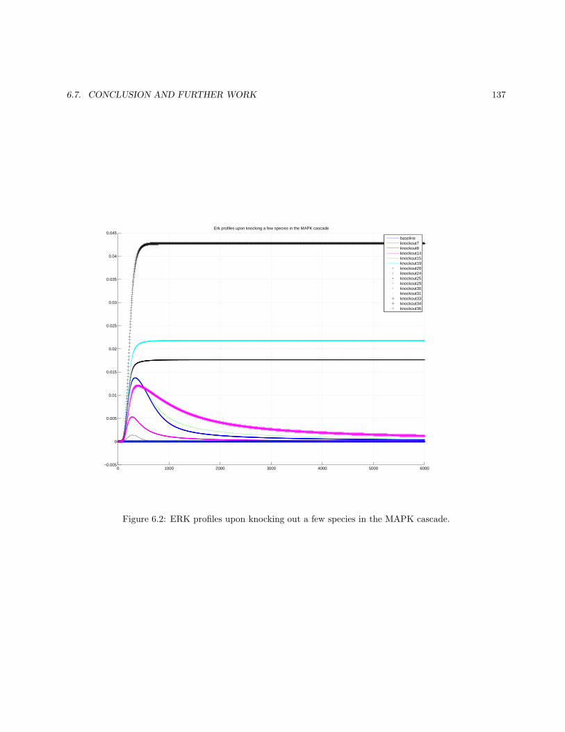
6.7. CONCLUSION AND FURTHER WORK 137
0 1000 2000 3000 4000 5000 6000−0.005
0
0.005
0.01
0.015
0.02
0.025
0.03
0.035
0.04
0.045Erk profiles upon knocking a few species in the MAPK cascade
baselineknockout7knockout8knockout14knockout15knockout19knockout20knockout24knockout25knockout29knockout30knockout31knockout33knockout34knockout36
Figure 6.2: ERK profiles upon knocking out a few species in the MAPK cascade.

138 CHAPTER 6. ANALYSIS OF BIOLOGICAL INTERACTION NETWORKS
Figure 6.3: Going from measures of ERK’s response to four knockout species to a matrix of measures of each
responder’s disruption by each knockout. mn represents one of the six measures. Measure values in this matrix
obtained by Maslova’s skew measure.

6.7. CONCLUSION AND FURTHER WORK 139
0 1 2 3 4 5 60
0.2
0.4
0.6
0.8
1(a)
Target
MM
Mai
n de
sire
d re
spon
se y
es/n
o
0 1 2 3 4 5 60
0.2
0.4
0.6
0.8
1(b)
Target
MT
Tot
al d
isru
ptio
n
0 1 2 3 4 5 60
0.2
0.4
0.6
0.8
1(c)
Target
MT
X T
otal
ext
ra d
isru
ptio
n be
yond
des
ired
resp
onse
0 1 2 3 4 5 60
0.2
0.4
0.6
0.8
1(d)
Targetnorm
1 T
otal
dis
rupt
ion
usin
g no
rmal
ized
one
nor
m
Figure 6.4: (a) Was the desied responder (ERK) significantly affected by knocking out the target? (MM
measure) (b) How much was the entire system affected by knockout of the target? (MT measure) (c) How
many “extra” disrupted responders, excluding ERK, resulted from each knockout? (MTX measure) (d) How
much was the entire system affected by knockout of the target? (norm1)

140 CHAPTER 6. ANALYSIS OF BIOLOGICAL INTERACTION NETWORKS
0 1 2 3 4 5 60
0.2
0.4
0.6
0.8
1
Target
MM
Mai
n de
sire
d re
spon
se y
es/n
o
(e) Softened threshold
0 1 2 3 4 5 60
0.2
0.4
0.6
0.8
1
Target
MT
Tot
al d
isru
ptio
n
(f) Softened threshold
0 1 2 3 4 5 60
0.2
0.4
0.6
0.8
1
Target
MT
X T
otal
ext
ra d
isru
ptio
n be
yond
des
ired
resp
onse
(g) Softened threshold
0 1 2 3 4 5 60
0.2
0.4
0.6
0.8
1
Target
Ext
ent o
f mai
n de
sire
d re
spon
se m
ispec
(h) ispec = 3
Figure 6.5: (e) Was the desired responder (ERK) significantly affected by knocking out the target? (MM
measure) (f) How much was the entire system affected by knockout the target? (MT measure) (g) How many
“extra” disrupted responders, exluding ERK, resulted from each knockout? (MTX measure) (h) How much
was the desired responder (ERK) affected by knocking out the target? (mispec)

6.7. CONCLUSION AND FURTHER WORK 141
0 1000 2000 3000 4000 5000 60000
0.1
0.2
0.3
0.4
0.5
0.6
0.7
0.8
0.9
1
time
various types of curves curve type 1curve type 2curve type 3curve type 4curve type 5curve type 6
0 1000 2000 3000 4000 5000 60000
0.002
0.004
0.006
0.008
0.01
0.012
0.014
0.016
time
1st and 2nd types of curves
Figure 6.6: The test curves.
0 1000 2000 3000 4000 5000 60000
0.5
1
time
The Blackman window centered at 390(location of max for curve 1) with width 600
Figure 6.7: The Blackman window weighted function.

142 CHAPTER 6. ANALYSIS OF BIOLOGICAL INTERACTION NETWORKS
0 1000 2000 3000 4000 5000 60000
0.1
0.2
0.3
0.4
0.5
0.6
0.7
0.8
0.9
1
time
The Tukey window centered at 4500 with width 1500 and taper−constant ratio 0.001
Figure 6.8: The Tukey window weighted function.

6.7. CONCLUSION AND FURTHER WORK 143
1 2 3 4 5 60
0.2
0.4
0.6
0.8
1
compared curve
relative L2 scale measures with uniform unit weight
curve 1 as basecurve 2 as basecurve 3 as basecurve 4 as basecurve 5 as basecurve 6 as base
1 2 3 4 5 60
0.2
0.4
0.6
0.8
1
compared curve
relative L2 scale measures with weight of Blackman window
1 2 3 4 5 60
0.2
0.4
0.6
0.8
1
compared curve
relative L2 scale measures with weight of Tukey window
Figure 6.9: The measures of scale changes in different weight functions.

144 CHAPTER 6. ANALYSIS OF BIOLOGICAL INTERACTION NETWORKS
1 2 3 4 5 60
0.1
0.2
0.3
0.4
0.5
0.6
0.7
0.8
0.9
1
compared curve
relative L2 shape change measures with uniform unit weight
curve 1 as basecurve 2 as basecurve 3 as basecurve 4 as basecurve 5 as basecurve 6 as base
1 2 3 4 5 60
0.1
0.2
0.3
0.4
0.5
0.6
0.7
0.8
0.9
1
compared curve
relative L2 shape change measures with Tukey window weight
Figure 6.10: The measures of relative shape changes in uniform unit weight and Tukey window weight focused
on second half domain.

6.7. CONCLUSION AND FURTHER WORK 145
1 2 3 4 5 6 7 8 9 1011121314151617181920212223242526272829303132333435360
0.1
0.2
0.3
0.4
0.5
0.6
0.7
0.8
0.9
1
knock out species
relative L2 scale changes
1 2 3 4 5 6 7 8 9 1011121314151617181920212223242526272829303132333435360
0.05
0.1
0.15
0.2
0.25
0.3
0.35
0.4
knock out species
relative L2 shape changes
Figure 6.11: The measures for relative scale change and relative shape change for the knockout response curves
with ERK as a responder. The weight function used was uniform unit weight.

146 CHAPTER 6. ANALYSIS OF BIOLOGICAL INTERACTION NETWORKS
0 5 10 15 20 25 30 350
0.1
0.2
0.3
0.4
0.5
0.6
0.7
0.8
0.9
1
Specis #
Rel
ativ
e ku
rtos
is
Relative kurtosis score for ERK knockout data
Figure 6.12: Difference of kurtosis scores for ERK knockout data.
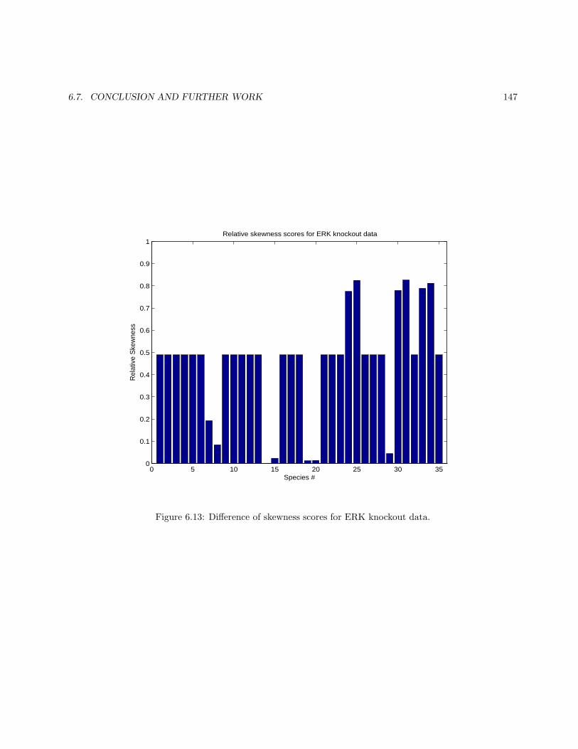
6.7. CONCLUSION AND FURTHER WORK 147
0 5 10 15 20 25 30 350
0.1
0.2
0.3
0.4
0.5
0.6
0.7
0.8
0.9
1
Species #
Rel
ativ
e S
kew
ness
Relative skewness scores for ERK knockout data
Figure 6.13: Difference of skewness scores for ERK knockout data.

148 CHAPTER 6. ANALYSIS OF BIOLOGICAL INTERACTION NETWORKS1 2 3 4 5 6 7 8 9 10 11 12 13 14 15 16 17 18 19 20 21 22 23 24 25 26 27 28 29 30 31 32 33 34 35 36
1
2
3
4
5
Classification
Figure 6.14: Classification that shows whether there was a sign change in skewness or not. Green color
indicates that skewness of the knockout data has changed the sign.

6.7. CONCLUSION AND FURTHER WORK 1491 2 3 4 5 6 7 8 9 10 11 12 13 14 15 16 17 18 19 20 21 22 23 24 25 26 27 28 29 30 31 32 33 34 35 36
1
2
3
4
5
Relative skewness value for class 1
Figure 6.15: Relative skewness of class 1, δX,Y = 1. White color here shows which elements belong to a
different class, hence it should be ignored.

150 CHAPTER 6. ANALYSIS OF BIOLOGICAL INTERACTION NETWORKS1 2 3 4 5 6 7 8 9 10 11 12 13 14 15 16 17 18 19 20 21 22 23 24 25 26 27 28 29 30 31 32 33 34 35 36
1
2
3
4
5
Relative skewness value for class 2
Figure 6.16: Relative skewness of class 2, δX,Y = 0. White color here shows which elements belong to a
different class, hence it should be ignored.
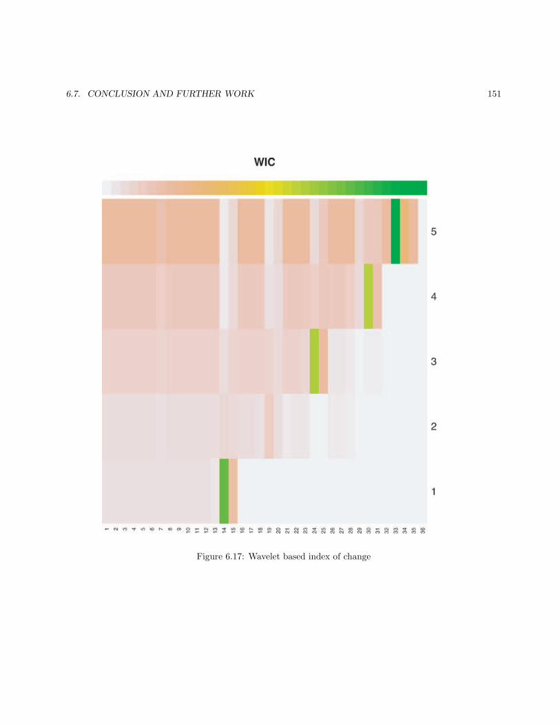
6.7. CONCLUSION AND FURTHER WORK 151
Figure 6.17: Wavelet based index of change
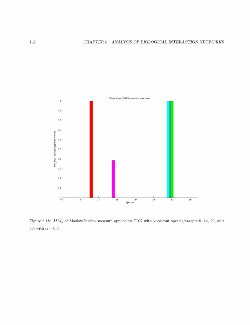
152 CHAPTER 6. ANALYSIS OF BIOLOGICAL INTERACTION NETWORKS
0 5 10 15 20 25 30 350
0.1
0.2
0.3
0.4
0.5
0.6
0.7
0.8
0.9
1
Species
MM
s Mai
n de
sire
d re
spon
se y
es/n
o
Disruption of ERK by species knock−out
Figure 6.18: MMs of Maslova’s skew measure applied to ERK with knockout species/targets 8, 14, 29, and
30, with α = 0.5.

6.7. CONCLUSION AND FURTHER WORK 153
0 5 10 15 20 25 30 350
0.1
0.2
0.3
0.4
0.5
0.6
0.7
0.8
0.9
1
Species
MT
X T
otal
ext
ra d
isru
ptio
n be
yond
des
ired
resp
onse
Disruption of entire system excluding ERK disruption
Figure 6.19: MTXs of Maslova’s skew measure applied to ERK with knockout species/targets 8, 14, 29, and
30, with α = 0.5.

154 CHAPTER 6. ANALYSIS OF BIOLOGICAL INTERACTION NETWORKS
0 2 4 6 8 10−100
−50
0
50
100Function
0 2 4 6 8 100
0.1
0.2
0.3
0.4Curvature
0 2 4 6 8 10−0.2
−0.1
0
0.1
0.2
0.3Curvature difference between x2
0 2 4 6 8 10−0.4
−0.3
−0.2
−0.1
0
0.1Curvature difference between log x
x2
−x2+25log x
log x
−x2+25log x
x2
log x
−x2+25log x
x2
log x
−x2+25log x
Figure 6.20: Four functions, their curvature, and the difference between curvatures.

6.7. CONCLUSION AND FURTHER WORK 155
0 2 4 6 8 10−100
−50
0
50
100Function
0 2 4 6 8 100
0.05
0.1
0.15
0.2
0.25Curvature absolute difference between x2
0 2 4 6 8 100
0.05
0.1
0.15
0.2
0.25
0.3
0.35Curvature absolute difference between log x
x2
−x2+25log x
log x
−x2+25log x
x2
log x
−x2+25log x
Figure 6.21: Four functions and the difference between the absolute curvatures.

156 CHAPTER 6. ANALYSIS OF BIOLOGICAL INTERACTION NETWORKS
6.8 Appendix
Additional possibilities to measure the difference between two curves:Shape is one aspect of the graph of a function that could differ from function to function. There are many
ways to describe shape, but one method is calculation of the curvature of the function. Recall that the secondderivative describes the convexity or concavity of a function’s graph. From calculus, the curvature κ of afunction can be derived, with the result
κ =|y′′|
(1 + (y′)2)(3/2)
Preliminary explorations of how curvature might distinguish between the graphs of two functions includeplotting the graphs of x2, log(x), −x2 + 2, and 5 log(x) and their curvatures. Then, first choosing a baselinefunction as x2 and second choosing a baseline function of log(x), the difference between the curvatures of eachfunction and the baseline, and the absolute value of the difference between the curvatures of each function andthe baseline were plotted graphically. A cursory examination indicates that curvature measures differences infunctions due to stretching and horizontal shifts but not vertical shifts (See Figures 6.20 and 6.21).

Bibliography
[1] Asthagiri, A. R. and Lauffenburger,D. A. (2001) A Computational Study of Feedback Effects on SignalDynamics in a Mitogen-Activated Protein Kinase (MAPK) Pathway Model, Biotechnol. Prog., 17:227-239.
[2] Percival, D. B. and Walden, A. T. (2000) Wavelet methods for time series analysis, Cambridge UniversityPress.
[3] http://www.bio.davidson.edu/courses/Immunology/Flash/MAPK.html
[4] http://biocreations.com/pages/mapk.html
[5] http://mathworld.wolfram.com/Kurtosis.html
[6] http://mathworld.wolfram.com/Skewness.html
[7] http://www.riskglossary.com/link/skewness.htm
[8] http://www.math.hawaii.edu/∼ lee/calculus/curvature.pdf
[9] http://itp.tugraz.at/matlab/toolbox/fuzzy/sigmf.html
157