Tutorial: RNA-Seq Analysis Part I...

Sample to Insight

Tutorial: RNA-Seq Analysis Part I (Tracks): Getting StartedFebruary 24, 2014

Tuto

rial

Tutorial: RNA-Seq Analysis Part I (Tracks): Getting Started

Tutorial: RNA-Seq Analysis Part I (Tracks): Getting StartedThis tutorial is the first part of a series of tutorials about RNA-seq. This tutorial series can beused with CLC Genomics Workbench 7.0 or later versions. If you are using an older version ofCLC Genomics Workbench, you should in stead choose to use the "RNA-Seq Analysis (Legacy)"tutorial series.

The purpose of the tutorial is to help you get acquainted with the CLC Genomics WorkbenchRNA-seq tool. We cover the basics steps of running an RNA-seq analysis and describe the typesof results produced. We also introduce you to how to navigate between the various result types.

The primary objective of the RNA-seq analysis tool is to produce mRNA expression levels forgenes and/or transcripts, from samples of (m)RNA reads. This is done by:

• Mapping the reads to either a reference genome that includes gene annotations and(optionally) mRNA annotations, or to a set of reference sequences (e.g. ESTs). Themapping results are output as a reads track.

• Summarizing the result of the mapping at the gene and transcript level, or the referencesequence level. This results in gene and transcript, or reference level expression tracks,that report expression values at the gene level, transcript level, or reference sequencelevel, respectively.

A track list can be created that contains the reads tracks and expression level tracks. Track listsare useful for navigating and investigating the results in detail.

In this tutorial we look at a simple situation where we analyze one sample.

Related tutorials: If you have analyzed several RNA-seq samples, an experiment can be set upfrom the expression tracks from these samples, and the expression patterns between the samplesin the experiment can be analyzed with the tools in the Transcriptomics Analysis toolbox. This isdescribed in the tutorial RNA-Seq Analysis Part III Tracks (http://www.clcbio.com/files/tutorials/RNA-Seq_analysis_part_III_tracks.pdf). The reads tracks can be ana-lyzed in detail (e.g. for variants, insertions and deletions) by using the tools in the Resequencingtoolbox. How to do this is described in other tutorials such as Resequencing Analysis usingTracks (http://www.clcbio.com/files/tutorials/Resequencing-and-tracks-chrM.pdf).

Download and import data

The data used is from a study reported in http://www.ncbi.nlm.nih.gov/pmc/articles/PMC2868100/. In the study the authors considered three types of mouse tissue: embryonicstem cells (ESC), neuronal precursor cells (NPC), and lung fibroblasts (LFB).

1. Download the sample data from our website: http://download.clcbio.com/testdata/MouseChr7dataset.zip

2. Start the CLC Genomics Workbench.

3. Import the data by going to the toolbar:

Import ( ) | Standard Import ( )

P. 2

http://www.clcbio.com/files/tutorials/RNA-Seq_analysis_part_III_tracks.pdf)

http://www.clcbio.com/files/tutorials/RNA-Seq_analysis_part_III_tracks.pdf)

http://www.clcbio.com/files/tutorials/Resequencing-and-tracks-chrM.pdf

http://www.clcbio.com/files/tutorials/Resequencing-and-tracks-chrM.pdf

http://www.ncbi.nlm.nih.gov/pmc/articles/PMC2868100/

http://www.ncbi.nlm.nih.gov/pmc/articles/PMC2868100/

http://download.clcbio.com/testdata/MouseChr7dataset.zip

http://download.clcbio.com/testdata/MouseChr7dataset.zip

Tuto

rial


4. Choose the zip file called MouseChr7dataset.zip. Leave the Import type set to Automatic.

Included in the dataset provided for this tutorial are

Reads from the ESC and NPC tissue samples There are sequence lists of reads from two bio-logical samples from the ESC and NPC tissue types. These read sets contain only thereads that map to chromosome 7. The sequence lists are called ESC-1, ESC-2, NPC-1, andNPC-2. In this tutorial, we consider only one of the ESC samples. The other ESC sampleand the NPC data are used in a later tutorial in this series1.

Mouse chromosome 7 genome reference and annotations

Once the data has been downloaded and imported, you should have the folders and data in theNavigation Area as shown in figure 1.

Figure 1: The chromosome 7 subset of the full data set has been imported.

Running the RNA-seq analysis

In this first RNA-seq tutorial we analyze one of the ESC samples using the RNA-seq analysis tool.That is, in this section, we will be making use of the following data:

• The sequence reads for the sample ESC-1

• The reference sequence for chromosome 7 of Mus musculus

• The annotated genes on chromosome 7 of Mus musculus (gene annotation track)

1To get the sequence lists containing reads that map to chromosome 7 only, we ran an analysis of the full data set(all reads and the full mouse genome) and then extracted all the reads that matched to chromosome 7 (including tomRNA annotations on chromosome 7). If we were to analyze the full data set, it would include mapping of 40 millionreads per sample to a 2.7 Gb genome (excluding transcripts), which would take too long for this tutorial.

P. 3

Tuto

rial


• The annotated transcripts on chromosome 7 of Mus musculus (mRNA annotation track)

1. To start the analysis of the ESC-1 sample, go to:

Toolbox | Transcriptomics Analysis ( ) | RNA-Seq Analysis ( ) | RNA-Seq Analysis( )

2. In the dialog, select the sequencing read list called ESC-1 by clicking on the Samplesfolder, then the ESC subfolder, then the ESC1 subfolder and finally, click on the ESC-1sequence list and then click on the arrow in the middle pointing to the right to have thisdataset included in the selected elements list at the right hand side. Double clicking onthe sequence list in the left hand side will also register it in the selected elements list (seefigure 2).

Figure 2: Selecting the ESC-1 sample for RNA-seq analysis.

3. Click on the button labeled Next.

Figure 3: Reference options.

At this point, we will specify which references to map the read sequences to (figure 3).We have a mouse sample and a reference sequence with gene and transcript annotationsavailable. Thus, we will choose the Genome annotated with genes and transcripts option.To analyze prokaryotic data, we would usually choose the Genome annotated with genesonly option. To analyze a sample from an organism for which no genome and gene

P. 4

Tuto

rial


annotations were available but where we had e.g. a list of ESTs, we would chose the Onereference sequence per transcript option.

4. Click the browse icon ( ) to the right of the "Reference sequence" area and browse tothe data item called "Mus musculus sequence" (see figure 4). Click on this item and thenclick on the arrow in the middle pointing to the right to have this dataset included in theselected elements list at the right hand side.

Figure 4: Select reference sequence.

5. Click on the button labeled OK.

6. Now click the browse icon ( ) to the right of the "Gene track" area and get the "Musmusculus_Gene" track from the "Tracks" folder. Click on this item and then click on thearrow in the middle pointing to the right to have this dataset included in the selectedelements list at the right hand side.


8. Now click the browse icon ( ) to the right of the "mRNA track" area and get the "Musmusculus_mRNA" track. Click on this item and then click on the arrow in the middle pointingto the right to have this dataset included in the selected elements list at the right handside.


We now need to specify which regions of the reference sequence the reads should bemapped to.

10. Choose the option: Map to gene regions only (fast) option.

With the selected references and parameter options, the Workbench will try to map readsto the reference regions covered by mRNA transcripts in the mRNA track and the referenceregions covered by gene annotations. Inter-genic regions of the reference are not used tomap the reads to in this case. The Also map to inter-genic regions option is considered ina later tutorial.


Now the parameters for the mapping of the reads to the reference can be set.

P. 5

Tuto

rial


Figure 5: Mapping options.

12. Leave all the parameters at their default values except for the Maximum number of hits fora read. Please set this to 1. See figure 5

Setting the Maximum number of hits for a read parameter to 1 means that only reads thatmap uniquely are considered. In other words, any read that maps equally well to two ormore genes or regions in a gene will not be considered. We will examine the effect of thisand other parameters in a later tutorial.

Hint If you have changed some of the values when running tasks in the Workbench andwould like to return to the default settings, just click the ( ) at the bottom of the wizardview. All settings in that particular wizard step are then changed to the defaults.

13. Click on the button labeled Next to go to the next wizard step.

At this point, we specify how we wish the mapped reads to be counted and which expressionvalue should be presented in the output. We can also specify whether we wish a particulartype of expression value, RPKM, to be calculated for genes without transcripts.

14. Leave the settings at this stage to the defaults. That is, neither checkbox is selected andthe expression value selected is Total counts (figure 6).

The options in this wizard step are described in full in the CLC Genomics Workbench manualstarting at:

http://www.clcsupport.com/clcgenomicsworkbench/current/index.php?manual=Calculating_expression_values_from_RNA_Seq.html

In brief:

Expression level options These parameters are related to how reads should be counted.The default option is to count the number of fragments. When you have paired reads, thetwo reads in a pair come from the same fragment and intact paired reads will be countedas one fragment. Broken pair reads are likely to be due to spurious mappings, and usingthis counting scheme would be ignored. Single reads would be indicative of one fragmentand under this scheme would thus be counted as one. The option to Count paired readsas two allows you to count reads rather than fragments. When this option is chosen, eachread, whether belonging to a paired read, a broken pair, or is a single read, is counted asone.

P. 6



Tuto

rial


Figure 6: Expression level options.

Expression value types specify what to put in the special column called "Expression value"in the gene and transcript level expression track. It is the values in this column thatare used when the expression tracks are colored using the heat-map-style. It is also thevalues in this column that a number of the "Transcriptomics Analysis" tools in the CLCGenomics Workbench Toolbox operate on. The choices for the gene level expression tracksare "RPKM", "Unique counts" or "Total counts".

RPKM is a special kind of expression measure that attempts to scale the counts for eachgene by both the total number of mapped reads in the sample and the length of the exonsof the gene. Some genes have no corresponding mRNA annotations, e.g. various types ofnon-coding genes. If you want RPKM values to be generated for the genes without mRNAannotations you check the Calculate RPKM for genes without transcripts box. When thisis done, the full length of the genes is used for genes without transcripts in place of the"total lengths of exons" in the RPKM value (see section "Definition of RPKM" later in thistutorial for an explanation of the RPKM expression measure).

Unique counts and Total counts refer to the counts of fragments or reads mapping toexon-regions of the gene.


At this point, the output options are specified as shown in figure 7.

The RNA-seq algorithm will always produce a reads track. It will also automatically producegene, transcript, or "reference" level expression tracks, depending on which option wasselected as "References" earlier, (figure 3). In this case we have specified both a geneand an mRNA track, and the algorithm will generate both a gene and a transcript levelexpression track. In addition to these automatically generated tracks, it is possible to geta report, a fusion-gene table and a list of the unmapped reads.

We want to make use of the report in a later tutorial, so:

16. Check the box next to Create report. Leave the options Create fusion gene table, Createlist of un-mapped reads, and Open log unchecked.

17. Click on the button labeled Save.

We now specify where to save the results to.

P. 7

Tuto

rial


Figure 7: Selecting the output of the RNA-seq analysis.

18. Browse to your "MouseChr7dataset" folder and add a new folder with the name "RNAseqanalysis". To add a new folder, just click on the Folder icon ( ) near the top of the wizardwindow.

19. Click on the button labeled Finish.

The RNA-seq analysis is now running. If you want to watch its progress, click on theProcesses tab in the bottom left side of the Workbench. The progress bar gives anindication of the stage that an analysis is at. In other words, it does not show the precisepercentage completion of a job, but indicate how far through the various stages you haveprogressed. For complex tasks like RNA-seq analysis, text above the progress bar willlet you know what stage is running, for example, stages like Mapping, Counting matches,Building mappings, Finalizing mappings, Saving results and so on.)

Interpreting the ESC-1 analysis results

After the RNA-seq analysis is finished, the four output types requested will be written to the"RNAseq analysis" folder you have created (see figure 8). In this section we review theseoutputs and how they can be viewed.

Figure 8: The outputs of the RNA-seq analysis.

20. We will now create a track list of the gene level expression track; ESC-1 (GE), the transcriptlevel expression track; ESC-1 (TE), and the reads track; ESC-1 RNA-seq (Reads).

One way to do this is by selecting the three tracks in the Navigation area, depressing theCtrl key so you can select multiple inputs, and then right clicking and selecting New in theright-click menu, and then Track List. This is shown in figure 9.

Another way to do this is to click Ctrl + L to start up the Track List wizard. Then browse tothe tracks you wish to include in that list and move them into the selected elements area,

P. 8

Tuto

rial


as you have done with data earlier in this tutorial.

You can rearrange the order of the tracks in a track list in the viewing area by clicking ona track name, and keeping the mouse button depressed, dragging the track vertically intothe place that you want it.

Figure 9: Creating a track list.

Figure 10: A tracklist containing the gene level expression track ESC-1 (GE), the transcript levelexpression track ESC-1 (TE) and the reads track ESC-1 RNA-seq (Reads) generated by the RNA-seqanalysis tool. The reads track shows the read mapping. Here, the zoom level is set such that weare seeing the coverage graph. Zooming in would allow us to view the mapped reads.

21. Double-click on the name of the gene level expression track "ESC-1 (GE)" within the tracklist. This opens the gene expression track as a table, shown in a split view below the tracklist. Opening the gene expression track this way means that the gene expression tracktable and the track list are linked. That is, if you select a row in the table by clicking on it,the track list will show that region.

22. Click on the "Expression value" column header of the gene expression track table twice toget the rows sorted descendingly by expression value.

P. 9

Tuto

rial


23. Click on the top row in the gene expression track table, that is, click on the row for thegene Ftl1.

When you clicked on the row for the gene Ftl1, a selection was made in the track listcorresponding to the region of the gene Ftl1. To see this more clearly:

24. Click on the zoom-to-selection icon ( ) at the bottom of the track list. The editor will nowzoom in on the selected region. You should now see something similar to figure 11.

Figure 11: The gene expression level track opened in a split view from the track list is linked tothe track list. Here the row for the Ftl1 gene was selected in the gene expression level track. Theregion corresponding to the gene is then automatically selected in the track list. By clicking the"zoom-to-selection" button, the view is moved to display the selected region.

At this zoom level you can see the individual reads mapped. Reads that are mapped inpairs are blue, and the individual reads in the pair are connected by a thin blue line. Forsome reads a thin dotted line connects each end of the read. These are the reads thathave been mapped across exon-exon boundaries.

For this particular gene, there are only reads mapped in intact pairs, so all reads visibleare blue. When there are single reads, these are colored green if they are mapped to theforward strand of the reference sequence and red if they are mapped to the reverse strand.Broken pair reads are colored red and green, like single reads, but here, less bright colorsare used. In the Side Panel in the right-hand side of the Workbench you can "disconnect"the reads that are mapped in pairs; Click on the "Disconnect paired reads" option in the"Reads track" section of the Track List Settings (figure 12). When you do that, the reads ina pair are colored green or red according to the reference strand to which they map. Reads

P. 10

Tuto

rial


that are mapped non-specifically (that is, that could equally well have been mapped to adifferent location) are colored yellow.

Figure 12: You can disconnect pairs in the Side Panel under in the right-hand side of the Workbenchunder "Reads track" by ticking "Disconnect paired reads".

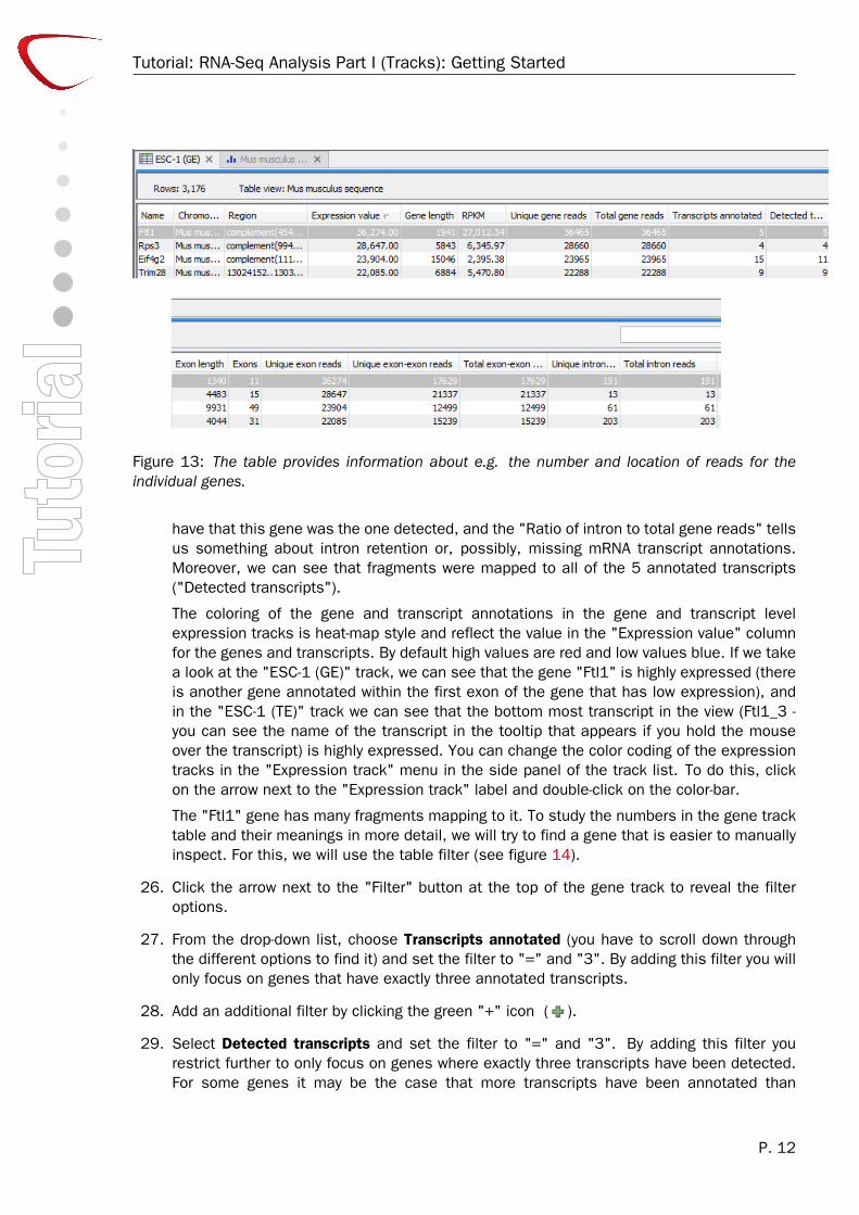
25. Now, take a look at the "ESC-1 (GE)" table as we are now going to examine the geneexpression level track "ESC-1 (GE)" more closely. The rows in the gene expression leveltrack table contains information about the gene and the numbers and types of fragmentsor reads mapping to the gene and its mRNA transcripts. Hence, the table can provideinformation about which chromosome the gene is located on ("Chromosome"), where it islocated ("Region"), what the length of the gene is ("Gene length"), how many transcripts inthe mRNA track that are corresponding to this gene ("Transcripts annotated"), the numberof exons the gene has ("Exons"), and their cumulative length ("Exon length"). Pleasenote that as we have only have used data from chromosome 7 in this example, the"Chromosome" column does not provide information about the chromosome number.

If we look at the Ftl1 gene (see figure 13), we can see that 36,465 fragments were mappedto this region ("Total gene reads") and all of them mapped uniquely to this region ("Uniquegene reads").

36,274 fragments mapped within the exons of the mRNA transcripts for the gene ("Totalexon reads" and "Unique exon reads"). In the run shown, 17,629 mapped across introns("Total exon-exon reads" and "unique exon-exon reads"). Although we run with Maximumnumber of hits for a read = 1, and hence only reads that map uniquely at the gene levelare used, there is some randomness to the assignment of reads among transcripts, andthe exon-exon read numbers in your run may deviate a little from this number, as a readmay in one run be assigned to a transcript for which it is an exon-exon read, and in anotherto a transcript for which it is mapped entirely within an exon (see the manual on RNA-seqanalysis for an in depth discussion of this). 191 mapped (at least partly) to introns ("Totalintron reads" and "Unique intron reads").

The "Ratio of unique to total (exon reads)" tells us something about the confidence that we

P. 11

Tuto

rial


Figure 13: The table provides information about e.g. the number and location of reads for theindividual genes.

have that this gene was the one detected, and the "Ratio of intron to total gene reads" tellsus something about intron retention or, possibly, missing mRNA transcript annotations.Moreover, we can see that fragments were mapped to all of the 5 annotated transcripts("Detected transcripts").

The coloring of the gene and transcript annotations in the gene and transcript levelexpression tracks is heat-map style and reflect the value in the "Expression value" columnfor the genes and transcripts. By default high values are red and low values blue. If we takea look at the "ESC-1 (GE)" track, we can see that the gene "Ftl1" is highly expressed (thereis another gene annotated within the first exon of the gene that has low expression), andin the "ESC-1 (TE)" track we can see that the bottom most transcript in the view (Ftl1_3 -you can see the name of the transcript in the tooltip that appears if you hold the mouseover the transcript) is highly expressed. You can change the color coding of the expressiontracks in the "Expression track" menu in the side panel of the track list. To do this, clickon the arrow next to the "Expression track" label and double-click on the color-bar.

The "Ftl1" gene has many fragments mapping to it. To study the numbers in the gene tracktable and their meanings in more detail, we will try to find a gene that is easier to manuallyinspect. For this, we will use the table filter (see figure 14).

26. Click the arrow next to the "Filter" button at the top of the gene track to reveal the filteroptions.

27. From the drop-down list, choose Transcripts annotated (you have to scroll down throughthe different options to find it) and set the filter to "=" and "3". By adding this filter you willonly focus on genes that have exactly three annotated transcripts.

28. Add an additional filter by clicking the green "+" icon ( ).

29. Select Detected transcripts and set the filter to "=" and "3". By adding this filter yourestrict further to only focus on genes where exactly three transcripts have been detected.For some genes it may be the case that more transcripts have been annotated than

P. 12

Tuto

rial


detected. By adding both filters we ensure that we only focus on genes with the samenumber of annotated and detected transcripts.

30. Click on the button labeled Filter.

31. Choose to sort on "Gene length" by clicking the column header for that column once, sothat the genes are sorted in ascending order by gene length.

Row number 2 is the row for the gene "Nupr1". This gene has a reasonable number offragments mapping to it and has three mRNAs annotated, which are all detected in thisanalysis. This seems to be a good candidate to examine further.

32. Click the row for the Nupr1 gene, and "zoom-to-selection" ( ).

Figure 14: The nupr1 gene.

The transcript level expression track "ESC-1 (TE)" shows the transcripts annotated for thegene (figure 14). The information in the gene table tells us that there are eight exons intotal for this gene. One transcript has only two exons. This transcript shares it’s intronwith one of the other transcripts, which has three exons. This three-exon transcript sharesits second intron with the third transcript, which is also a three exon transcript. For the"Nupr1" gene there are 3 "Intron reads". Those are the reads that map, at least partly,within the first intron. The other intronic regions are also exonic regions of other transcripts.

P. 13

Tuto

rial


According to the table there are 40 exon-exon reads. These are the reads with dashedlines connecting the ends of the reads. Note that we are counting fragments, and there arethree paired reads where both reads in the pair are mapped across exon-exon junctions.Remember that these paired reads only contribute a value of 1 each to the fragment count.In addition to these three paired reads, there are 37 other paired reads where one of thereads is mapped across an exon-exon junction. There are 34 paired reads where eachread in the pair is mapped entirely within an exon. So altogether there are 74 "Total exonreads".

Next we will examine the transcript level expression track.

33. Double-click on the name of the track ESC-1 (TE) in the track list.

The track opens as a table in the split view (figure 15).

34. Filter to see only the rows relating to the "Nupr1" gene by typing "nupr1" in the filter textfield. Click on the second row (Nupr1_2).

35. Click "zoom-to-selection" ( ).

Figure 15: The nupr1 gene: transcript level expression.

We first focus on the "Nupr1_2" transcript. According to the table, this transcript has fourunique transcript reads. The reads that can be uniquely assigned to this particular transcriptare the reads that fall within the region 126,625,034 to 126,625,322 (the second intronicregion).

P. 14

Tuto

rial


The reads that uniquely distinguish the transcript "Nupr1_3" from the other two transcriptsare reads that map across the third intronic region. There is just one such read.

For the transcript "Nupr1_1" the situation is a bit more complex and we need to consider theexpected distance between reads in a pair. This distance was estimated by the algorithmand the estimated distances are reported in the "History" of the results. To see the history,click the ( ) at the bottom of the "ESC-1 (GE)" table. The estimated expected distancesbetween the reads in a pair is between 141 and 371 bp. By considering these restrictionsyou can see that the paired reads mapping on either side of the second intronic regionthat have their first read mapped across the first exon-exon junction must come from the"Nupr1_1" transcript and not the "Nupr1_2" transcript. In addition the paired reads thatmap across both the first and second introns can be uniquely assigned to the "Nupr1_1"transcript. This is the same for reads that map across the second exon-exon junction, andextend further to the left than the first exon of the "Nupr1_3" transcript.

It might be hard at this zoom level to distinguish which reads extend further to the left thanthe first exon of the "Nupr1_3" transcript.

36. To zoom in further on this region, go into "selection mode" and at the top of the track list,select the region around the start of the first exon for the "Nupr1_3" transcript.

37. Click on the zoom-to-selection ( ) tool.

If you have selected a small enough region, you will see the individual nucleotides in thereads, as shown in figure 16.

Figure 16: The nupr1 gene: zoomed in to single base resolution.

If not you cannot see the individual nucleotides, try zooming in a bit more.

P. 15

Tuto

rial


You can then see where there are mismatches, insertions or deletions in the reads relative to thereference. Here, most of the mismatches seem randomly scattered. However, one "G" variantseems to occur at the same position in many reads, and could be caused by the sample carryinga heterozygous allele at this position. The tools in the Resequencing section of the WorkbenchToolbox can help you identify variants in read mappings. These tools are not covered in theRNA-seq tutorial series.

Below, the RPKM value is described in more detail. For more advanced analysis of RNA-seqsamples please see the other tutorials in this series.

Definition of RPKMRPKM, Reads Per Kilobase of exon model per Million mapped reads, is defined in this way[Mortazavi et al., 2008]:

RPKM =total exon reads

mapped reads(millions)× exon length (KB).

Total exon reads This value can be found in the column with header Total exon reads in theexpression track. This is the number of reads that have been mapped to exons (eitherwithin an exon or at the exon junction). When the reference genome is annotated with geneand transcript annotations, the mRNA track defines the exons, and the total exon reads arethe reads mapped to all transcripts for that gene. When only genes are used, each gene inthe gene track is considered an exon. When an un-annotated sequence list is used, eachsequence is considered an exon.

Exon length This is the number in the column with the header Exon length in the expressiontrack, divided by 1000. This is calculated as the sum of the lengths of all exons (seedefinition of exon above). Each exon is included only once in this sum, even if it is presentin more annotated transcripts for the gene. Partly overlapping exons will count with theirfull length, even though they share the same region.

Mapped reads The sum of all mapped reads as listed in the RNA-Seq analysis report. Pleasenote that the option to Map to gene regions only will affect the number of mapped reads,since all intergenic reads will not be mapped if this option is selected. This means thatcomparison of RPKM values between samples should only be carried out if this parameterwas set in the same way for all samples.

P. 16

Tuto

rial

Bibliography

[Mortazavi et al., 2008] Mortazavi, A., Williams, B. A., McCue, K., Schaeffer, L., and Wold,B. (2008). Mapping and quantifying mammalian transcriptomes by rna-seq. Nat Methods,5(7):621--628.

17

Tutorial: RNA-Seq Analysis Part I...

Documents

Transcript of Tutorial: RNA-Seq Analysis Part I...