Tutorial:  Modeling a Centrifugal Compressor Using the Single Reference Frame (SRF) Model  Introduction  Centrifugal compressors are used to achieve a high pressure rise in a single stage, and are commonly seen in aircraft and automotive engines, power generation systems, and gas processing applications.  Computational fluid dynamics is used extensively in the design and analysis of compressors, with the aim of achieving high efficiency for a target pressure rise and flow rate range.  The purpose of this tutorial is to illustrate how to set up a centrifugal compressor model in ANSYS FLUENT.  This example represents the Single Reference Frame (SRF) modeling approach for single blade row turbomachinery analysis, as the entire computational domain is referred to a moving reference frame.  In this tutorial you will: 

• Use the SRF modeling with the density‐based solver and Spalart‐Allmaras turbulence model to solve for the compressor flow field. 

• Use periodic boundary conditions. 

• Define the turbo topology so that turbo post‐processing can be applied to the results.  Prerequisites  This tutorial assumes that you are familiar with the menu structure in FLUENT. The SRF capability of FLUENT is used in this tutorial. For more information on SRF modeling, refer to Tutorial 7: Using a Single Rotating Reference Frame of the ANSYS FLUENT 13 Tutorial Guide.  Problem Description  The problem involves modeling the steady‐state flow of air through a centrifugal compressor running at 14,000 rpm. There are 20 blade rows (a blade row is a passageway between two adjacent blades on the rotor) in this compressor.  To simplify the CFD calculation, the flow is modeled only through a single blade row and uses rotationally periodic boundary conditions on the boundaries between the blade rows.  The governing equations are cast in a SRF moving at the speed of the rotor. Air is treated as an ideal gas with constant values of specific heat, thermal conductivity, and dynamic viscosity. The schematic of a single blade row and the complete rotor (repeating a single blade row 20 times) are shown in Figures 1 and 2 respectively. 

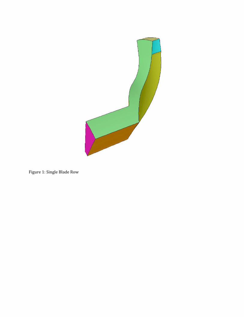
Figure 1: Single Blade Row 

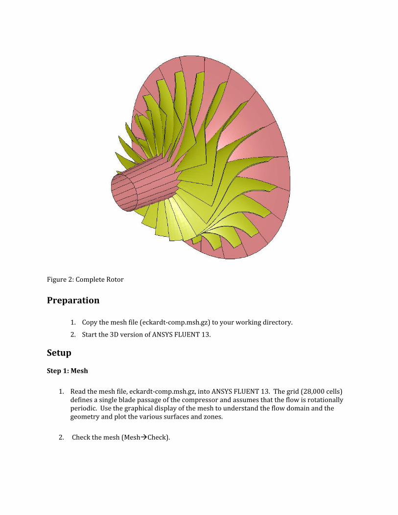
 Figure 2: Complete Rotor  Preparation  

1. Copy the mesh file (eckardt‐comp.msh.gz) to your working directory. 2. Start the 3D version of ANSYS FLUENT 13. 

 

Setup   Step 1: Mesh  

1. Read the mesh file, eckardt‐comp.msh.gz, into ANSYS FLUENT 13.  The grid (28,000 cells) defines a single blade passage of the compressor and assumes that the flow is rotationally periodic.  Use the graphical display of the mesh to understand the flow domain and the geometry and plot the various surfaces and zones. 

 

2.  Check the mesh (Mesh Check).  

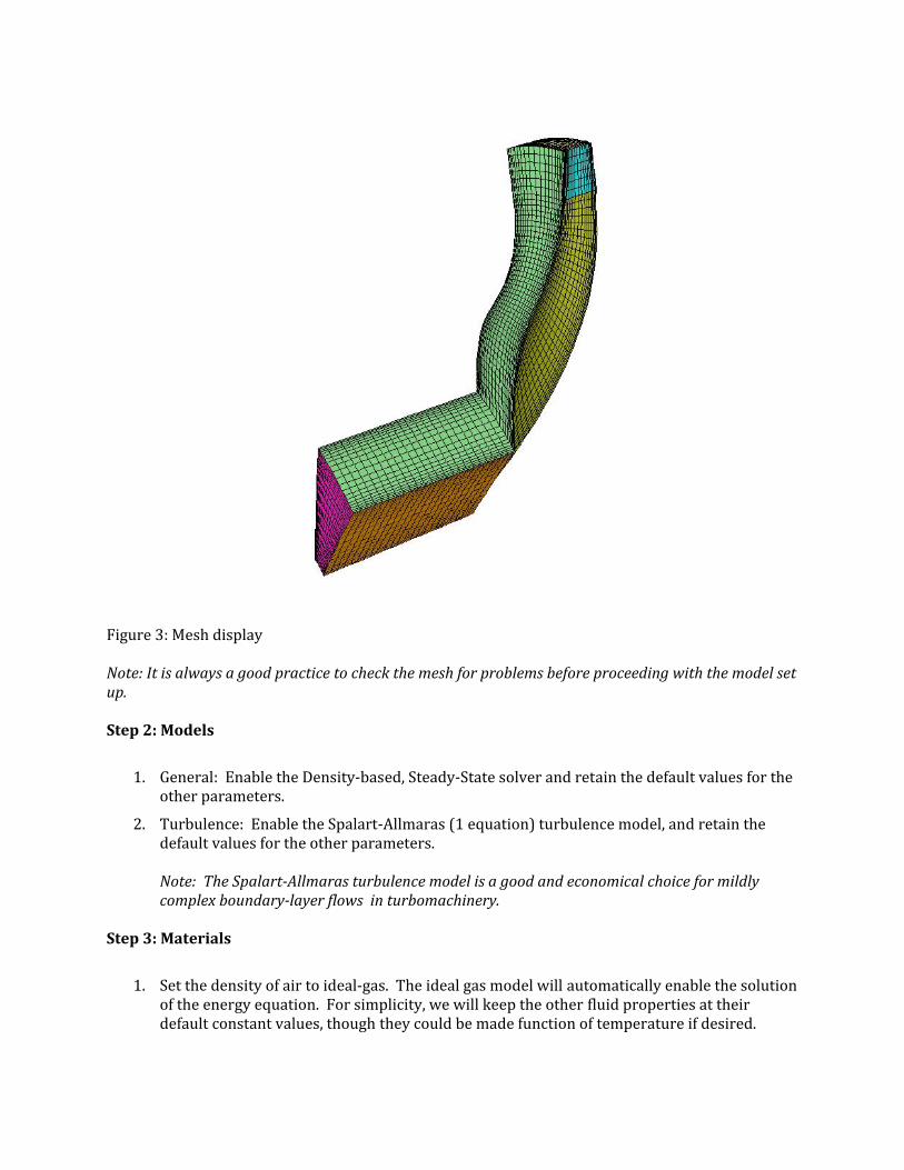
 Figure 3: Mesh display  Note: It is always a good practice to check the mesh for problems before proceeding with the model set up.  Step 2: Models  

1. General:  Enable the Density‐based, Steady‐State solver and retain the default values for the other parameters. 

2. Turbulence:  Enable the Spalart‐Allmaras (1 equation) turbulence model, and retain the default values for the other parameters. 

   Note:  The Spalart­Allmaras turbulence model is a good and economical choice for mildly   complex boundary­layer flows  in turbomachinery.  Step 3: Materials  

1. Set the density of air to ideal‐gas.  The ideal gas model will automatically enable the solution of the energy equation.  For simplicity, we will keep the other fluid properties at their default constant values, though they could be made function of temperature if desired. 

 

Step 4: Operating Conditions  

1. Set the Operating Pressure to 0 Pa, and retain the default values for the other parameters.    Note:  With the operating pressure set to zero, all the pressures will be absolute pressures.    This simplifies the specification pressures for compressible flows in the boundary conditions   panels.  Step 5: Cell Zone Conditions 

 

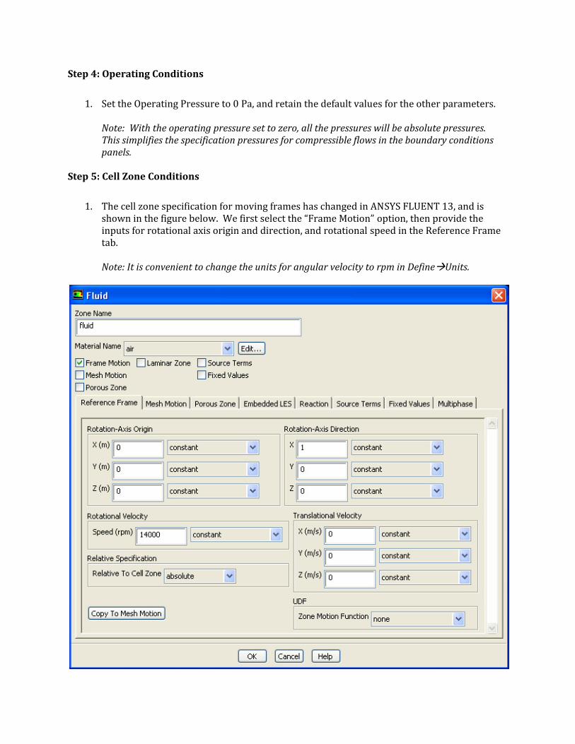
1. The cell zone specification for moving frames has changed in ANSYS FLUENT 13, and is shown in the figure below.  We first select the “Frame Motion” option, then provide the inputs for rotational axis origin and direction, and rotational speed in the Reference Frame tab.  

   Note: It is convenient to change the units for angular velocity to rpm in Define Units.  

 

  Step 6: Boundary Conditions  

1.  Set the boundary conditions for the zone inlet, which is a pressure inlet.  To facilitate the pressure inputs, change the units of pressure to atmospheres (atm) in Define Units. 

 

• Set the Gauge Total Pressure and Supersonic/Initial Gauge Pressure to 1 atm and 0.9   atm respectively. 

• Set the Total Temperature to 288.1 under the Thermal tab. 

• Set Turbulent Viscosity Ratio as the Specification Method for turbulence and the   value to 10. 

 

2. Set the boundary conditions for the zone outlet as follows:  

• Set the Gauge Pressure to 1.59. 

• Set the Backflow Total Temperature to 288 K. 

• Set the Backflow Direction Specification Method as From Neighboring Cell. 

• Set Turbulent Viscosity Ratio as the Turbulence Specification Method.   

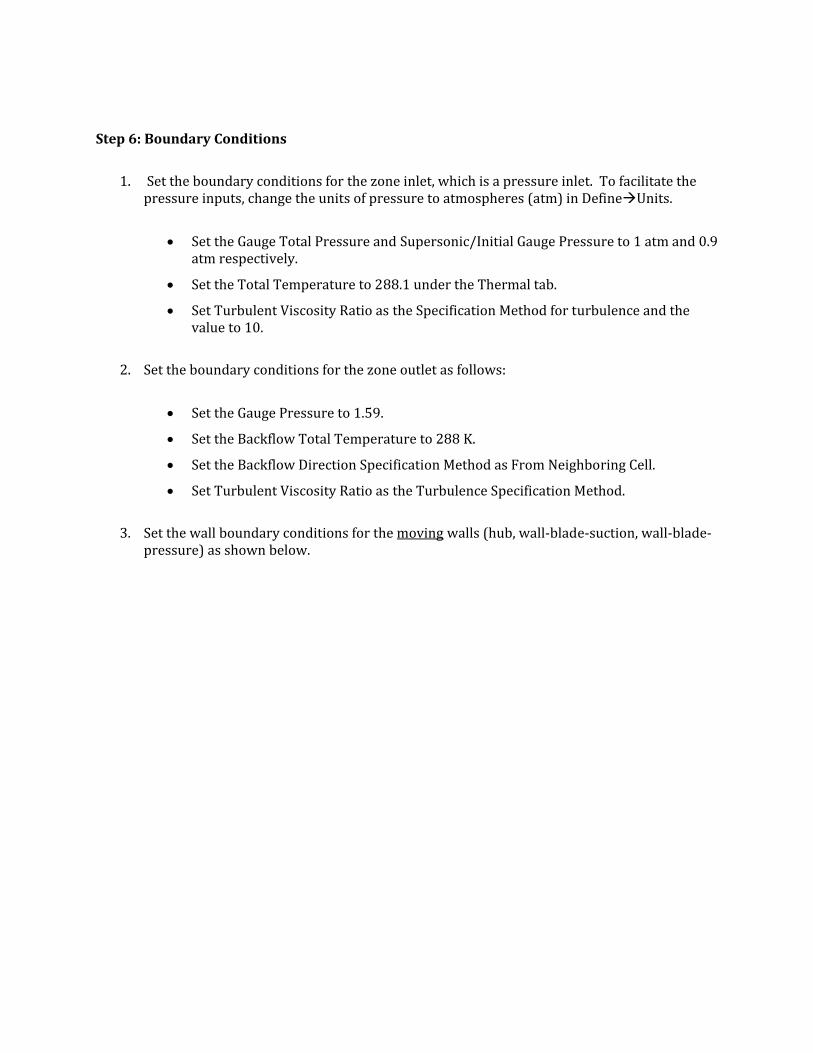
3. Set the wall boundary conditions for the moving walls (hub, wall‐blade‐suction, wall‐blade‐pressure) as shown below. 

 

  

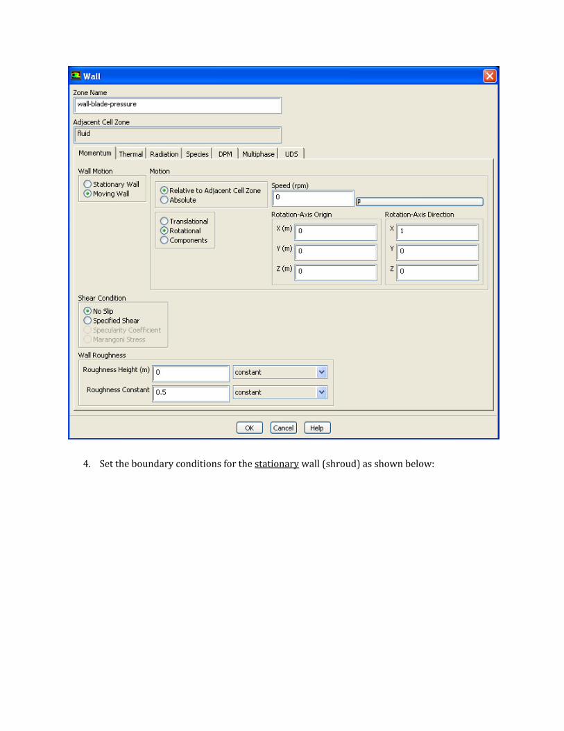
4. Set the boundary conditions for the stationary wall (shroud) as shown below:  

  

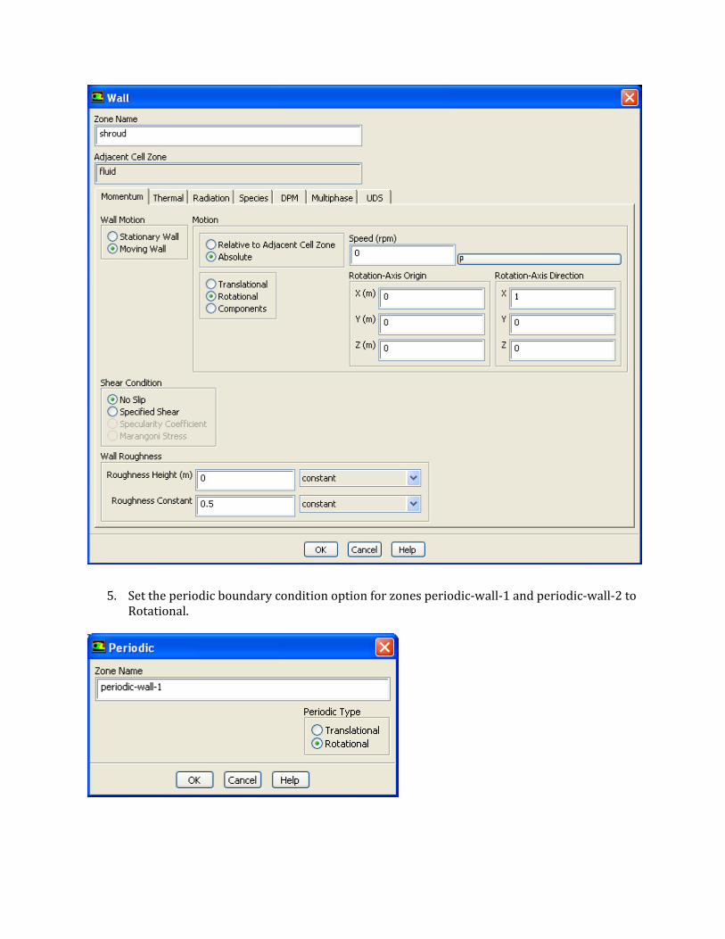
5. Set the periodic boundary condition option for zones periodic‐wall‐1 and periodic‐wall‐2 to Rotational. 

 

   

  Note:  The mesh file used in the present case has the periodic matching defined.  If you are   using a mesh from a source which does not defined the periodic matching, and the   corresponding nodes match one­for­one, you can create the periodic zones using the TUI   command mesh/modify­zones/make­periodic .  If the mesh does not match, you can create a   non­conformal periodic boundary condition using Define Mesh Interfaces.     Step 7: Solver Discretization, Controls, and Monitors  

1. Retain the default solution methods for flow under Solve Methods, and set the turbulence equation to Second Order Upwind.  Activate the Pseudo Transient method. 

2. Retain the default solution controls under Solve Controls. 

3. For the residual convergence, set the convergence criterion for Continuity to 1e‐4.  

4. Create three surface monitors as follows: 

• Mass flow rate at the inlet 

• Mass flow rate at the outlet 

• Mass‐averaged total pressure at the outlet.    Note: These surface monitors will be used to assess the convergence of the solution.  Step 8: Initialization  

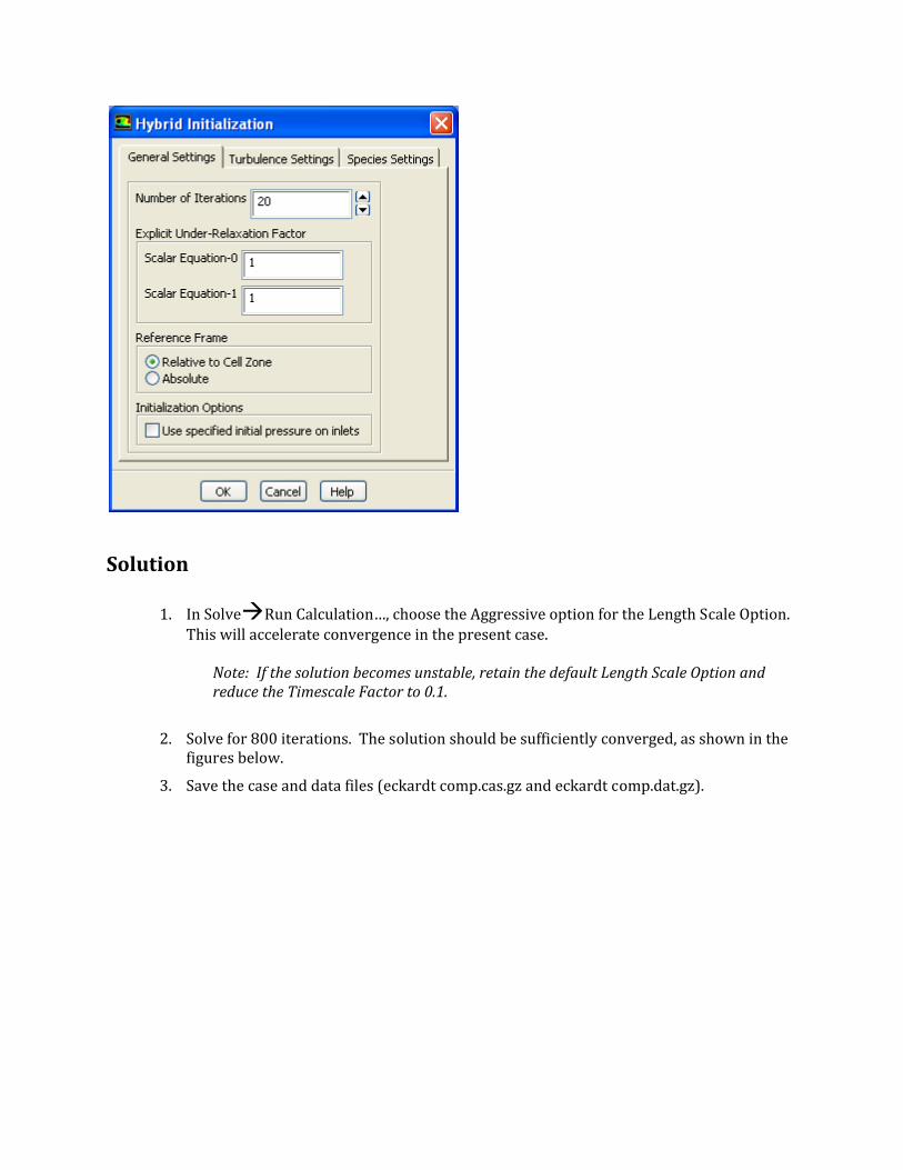
1. Use the hybrid initialization option (new in ANSYS FLUENT 13) to initialize the flow field. 

• Before initializing, click on the More Settings… button and enter 20 for the Number of Iterations as shown below. 

• Close the panel and click on Initialize.      Note: The convergence of the hybrid initialization will be printed to the text        interface. 

   Solution   

1. In Solve Run Calculation…, choose the Aggressive option for the Length Scale Option.  This will accelerate convergence in the present case. 

     Note:  If the solution becomes unstable, retain the default Length Scale Option and      reduce the Timescale Factor to 0.1.  

2. Solve for 800 iterations.  The solution should be sufficiently converged, as shown in the figures below. 

3. Save the case and data files (eckardt comp.cas.gz and eckardt comp.dat.gz).   

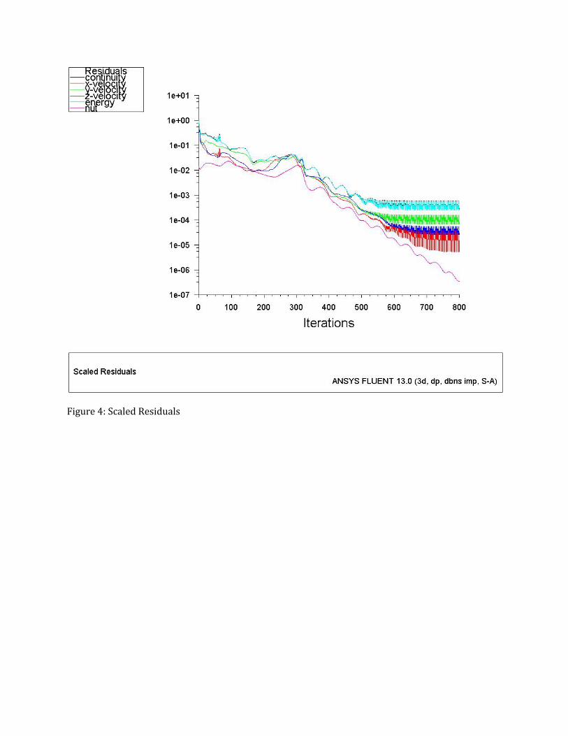
  Figure 4: Scaled Residuals 

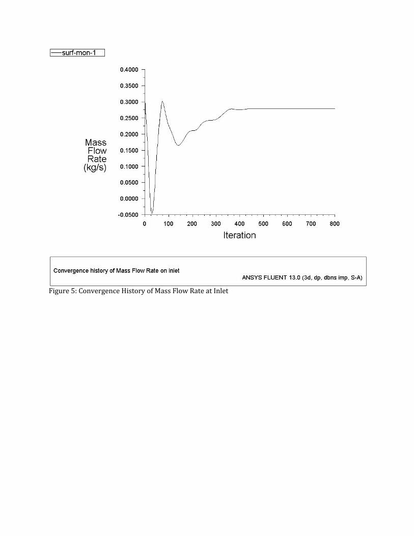
 Figure 5: Convergence History of Mass Flow Rate at Inlet  

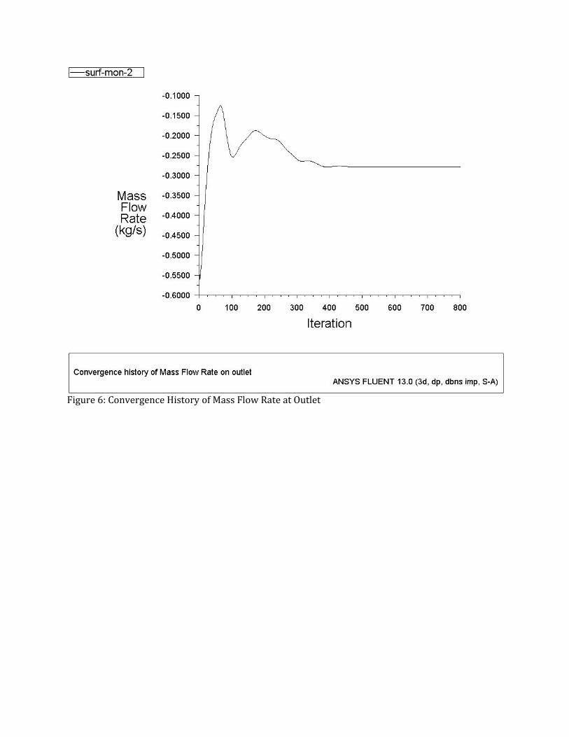
 Figure 6: Convergence History of Mass Flow Rate at Outlet  

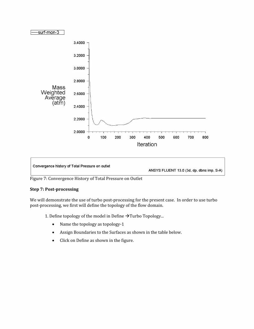
 Figure 7: Convergence History of Total Pressure on Outlet  Step 7: Post­processing  We will demonstrate the use of turbo post‐processing for the present case.  In order to use turbo post‐processing, we first will define the topology of the flow domain.    1. Define topology of the model in Define  Turbo Topology... 

• Name the topology as topology‐1 

• Assign Boundaries to the Surfaces as shown in the table below. 

• Click on Define as shown in the figure.  

   

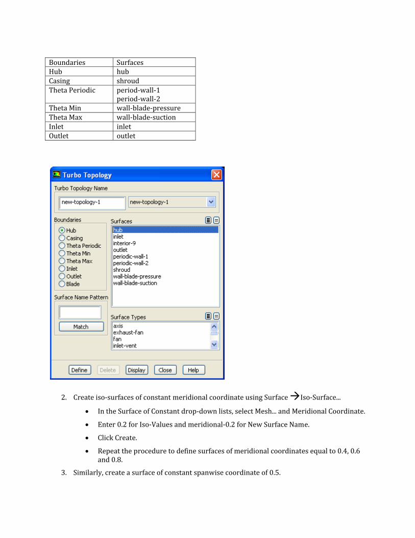
 Boundaries  Surfaces Hub  hub Casing  shroud Theta Periodic  period‐wall‐1 

period‐wall‐2 Theta Min  wall‐blade‐pressureTheta Max  wall‐blade‐suctionInlet  inlet Outlet  outlet    

  

2. Create iso‐surfaces of constant meridional coordinate using Surface  Iso‐Surface... 

• In the Surface of Constant drop‐down lists, select Mesh... and Meridional Coordinate. 

• Enter 0.2 for Iso‐Values and meridional‐0.2 for New Surface Name. 

• Click Create. 

• Repeat the procedure to define surfaces of meridional coordinates equal to 0.4, 0.6 and 0.8. 

3. Similarly, create a surface of constant spanwise coordinate of 0.5.  

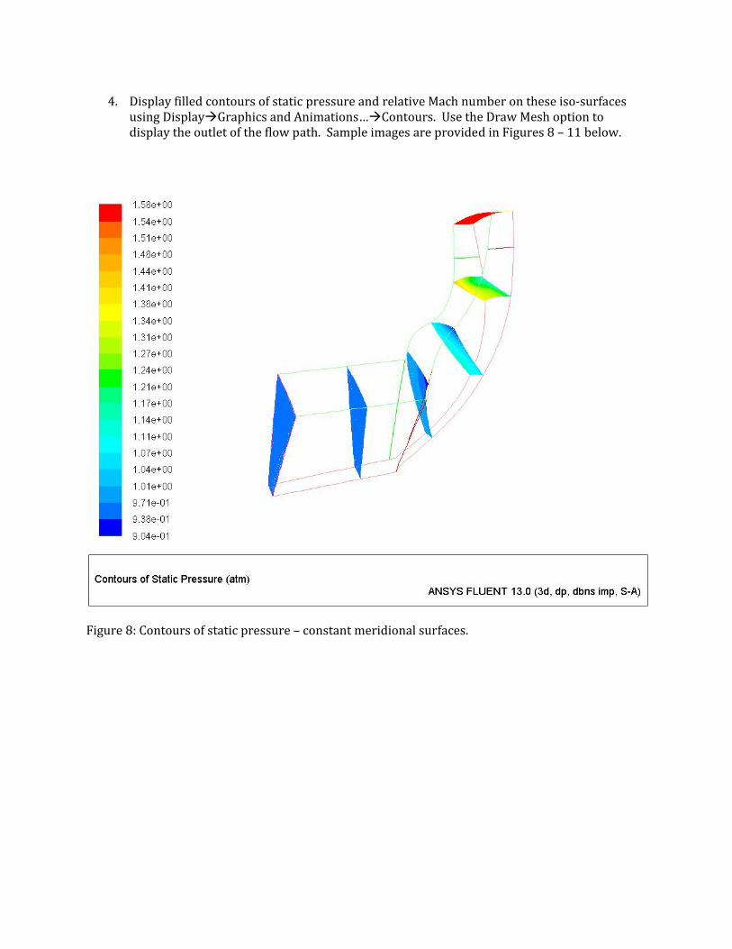
4. Display filled contours of static pressure and relative Mach number on these iso‐surfaces using Display Graphics and Animations… Contours.  Use the Draw Mesh option to display the outlet of the flow path.  Sample images are provided in Figures 8 – 11 below.   

 

  Figure 8: Contours of static pressure – constant meridional surfaces.  

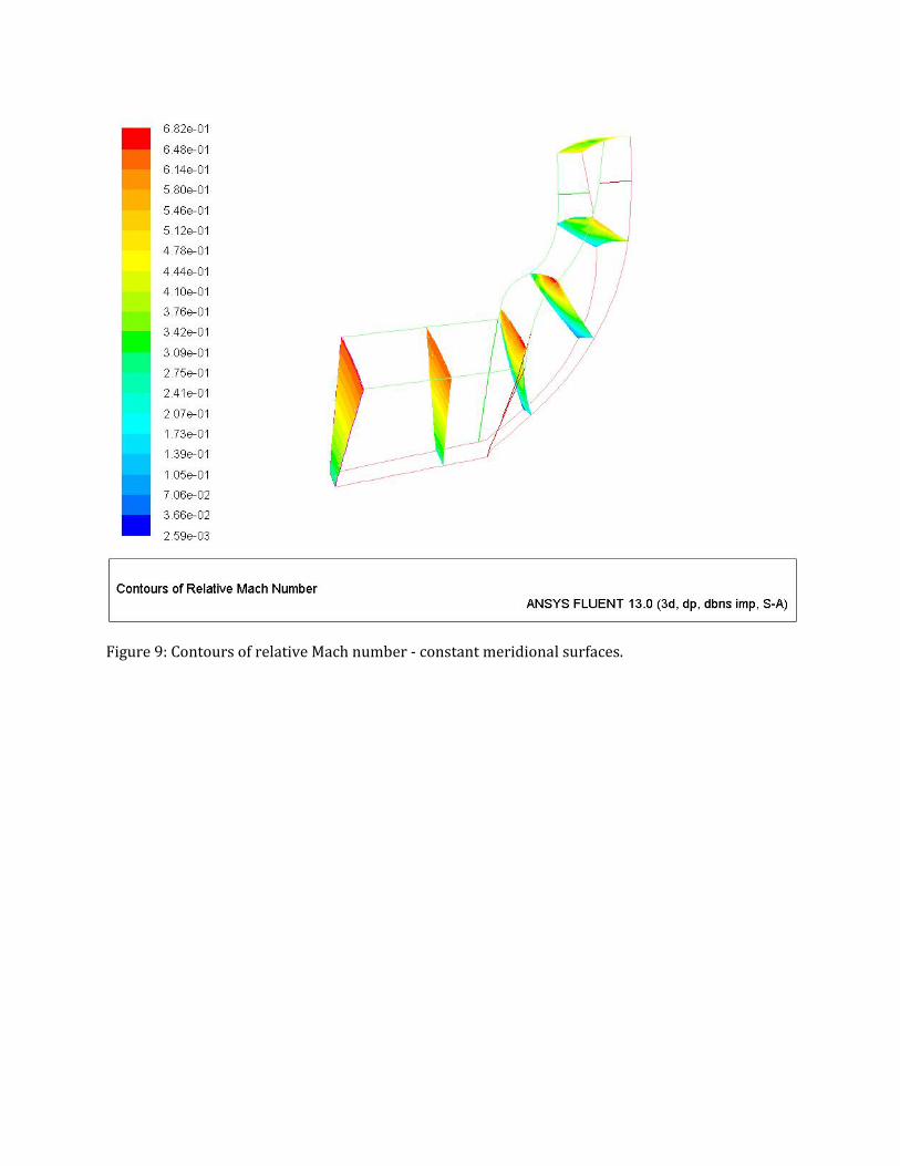
  Figure 9: Contours of relative Mach number ‐ constant meridional surfaces.  

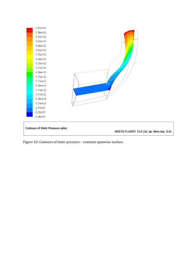
  Figure 10: Contours of static pressure – constant spanwise surface.  

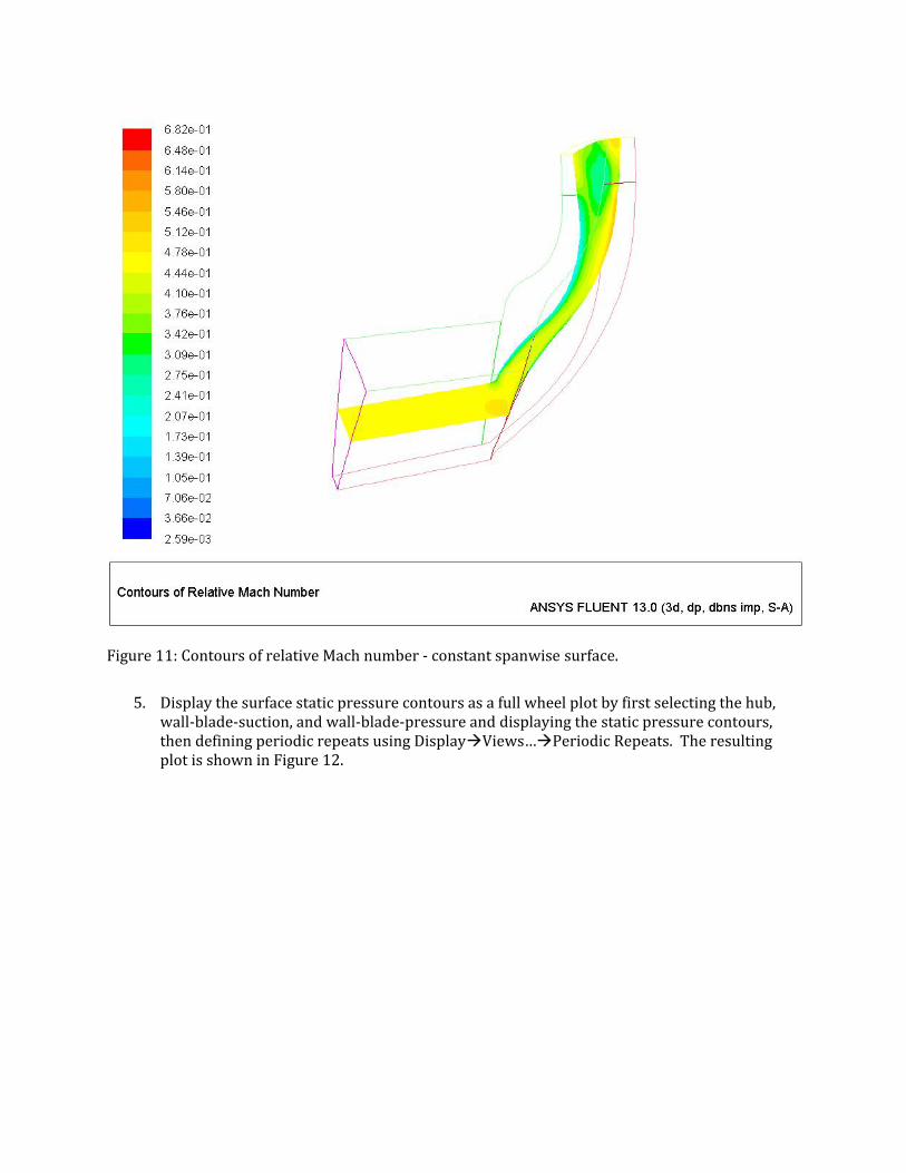
  Figure 11: Contours of relative Mach number ‐ constant spanwise surface.  

5. Display the surface static pressure contours as a full wheel plot by first selecting the hub, wall‐blade‐suction, and wall‐blade‐pressure and displaying the static pressure contours, then defining periodic repeats using Display Views… Periodic Repeats.  The resulting plot is shown in Figure 12. 

 

   

 

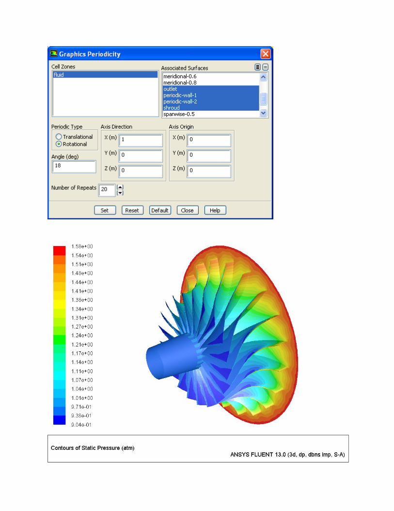
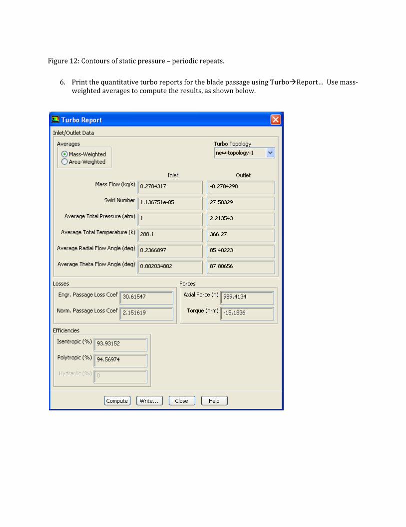
 Figure 12: Contours of static pressure – periodic repeats.  

6. Print the quantitative turbo reports for the blade passage using Turbo Report…  Use mass‐weighted averages to compute the results, as shown below.   

     

Summary  In this tutorial, we considered the SRF modeling for a single blade row turbomachinery analysis of a centrifugal compressor.   The density‐based solver was used to compute the solution, and turbo‐post‐processing tools were used to examine the solution and report quantitative data.  Additional analysis of the present blade row could be performed to examine the performance of the compressor over a range of rotational speeds and pressure ratios, which would yield an estimate of the compressor map for this design.  References  Eckardt, D., “Flow field analysis of radial and backswept centrifugal compressor impellers, Part I : Flow measurements using a laser velocimeter,” ASME 25th Annual International Gas Turbine Conference, March 9‐13, 1988.