Tutorial: Methods for assessing functional responses to ... · PDF fileTutorial: Methods for...

Tutorial: Methods for assessing functional

responses to environmental gradients

Kleyer et al.

June 22, 2009

This tutorial presents the different methods used in the paper. Ashort description of each method is given. We describe the proce-dures to carry out the analyses using the R language and interpretthe results.

Contents

1 Preliminary steps 2

2 Species responses to environmental gradients 3

3 A-”CWM-RDA”: redundancy analysis of community weightedmean trait responses to environmental gradients 4

4 B-”CLUS-MOD”: modelling functional groups on environmen-tal gradients 6

5 C-”RDA-sRTA”and D-”RDA-mRTA”: redundancy analysis andregression tree 14

6 E-”OMI-GAM”: outlying mean index and generalised additivemodel 23

7 F-”RLQ”: RLQ Analysis 32

8 G-”Double CCA”: double canonical correspondence analysis 39

1

1 Preliminary steps

1.1 Reading the data

The data corresponding to the three tables R (sites-by-environmental variables),L (sites-by-species) and Q (species-by-traits) are available in three text files(TAB-separated). The function read.table is used to read the data.

> traits <- read.table(file="data/Species_traits.txt", sep="\t")> spe<- read.table(file="data/Site_species.txt", sep="\t")> env<-read.table("data/Site_env.txt", sep="\t")

1.2 Sourcing the files with R code (functions)

> source("scripts/Inference_modelset.r")> source("scripts/Inference_compute.r")> source("scripts/corratio.R")> source("scripts/calinski.R")> source("scripts/VarScoreOMI.r")> source("scripts/doublerda.R")

1.3 Loading R packages

Several packages must be installed and loaded to perform the analyses presentedin this tutorial:> library(ade4)> library(MASS)> library(vegan)> library(ecodist)> library(maptools)> library(rpart)> library(splines)> library(gam)> library(pgirmess)> library(utils)> library(combinat)> library(mvpart)> library(cluster)> library(fpc)> library(clusterSim)> library(lmtest)> library(Hmisc)> library(gplots)

Other packages are also required by the different scripts associated to this tu-torial.

2

2 Species responses to environmental gradients

As a baseline, we analysed the responses of species to environmental gradientsusing canonical correspondence analysis (ter Braak, 1986). This analysis wasperformed using CANOCO for Windows 4.5 in the article and reproduced usingthe R language in this tutorial. We used the pcaiv function of the ade4 packagebut other functions are also available in other packages (e.g., cca function inpackage vegan).

> coa1 <- dudi.coa(spe, scannf = F)> cca1 <- pcaiv(coa1, env, scannf = F)

The percentage of variation in species composition explained by the threeenvironmental variables:> 100 * sum(cca1$eig) / sum(coa1$eig)

[1] 14.89

The species responses can be interpreted on the biplot (this corresponds toFigure 2 of the article).

> s.label(cca1$c1, clabel = 0)> par(mar = c(0.1, 0.1, 0.1, 0.1))> pointLabel(cca1$c1,row.names(cca1$c1), cex=0.7)> s.arrow(cca1$cor[-1,], add.plot=TRUE)

d = 1

●

●

●

●

●

●

●

●

●

●

●

●

●

●

●

●

●

●

●

●

●●

●

●

●

●

●

●

●

●

●

●●

●

●

●

●

●

●

●

●

●

●

●

●

●

●

●

●

●

ACHIMILL

AGROCAPI

ANTHODOR

BRIZMEDI

BROMHORD

CAPSBURS

CAREFLAC

CAREHIRT

CARENIGR

CENTJACE

CERAARVE

CERAGLOM

CIRSARVE

CYNOCRIS

DAUCCARODESCCESP.CES

EQUIPALU

FESTOVIN

FESTPRAT

FESTRUBR

GALIMOLL

GALIULIG

HIERACIU

HOLCLANA

HYDRVULG

LEONAUTU

LOLIPERE

LOTUULIG

LUZUCAMP

MATRMARI.INO

MOLICAER

PHRAAUST

PLANLANC

POA_ANNU

POTEANSE

POTEEREC

POTEREPT

RANUACRI

RANUREPERUBUIDAE

RUMEACETOSEL

SENEJACO

STELGRAM

TRIFARVE

TRIFPRAT

TRIFREPE

VEROARVE

VEROCHAM

VICICRAC

VIOLTRIC

dist.int

SOIL.P

SOIL.WHC

3

3 A-”CWM-RDA”: redundancy analysis of com-munity weighted mean trait responses to en-vironmental gradients

3.1 Description of the method

A sites-by-traits matrix for analysis of trait-environment relationships was cre-ated from the original L matrix (species-by-sites) and Q matrix (species-by-traits). This matrix was weighted by abundance so that each entry in thematrix was the weighted mean of the trait values of all species present in thatsite (for continuous traits) or the weighted proportion of species with a categor-ical trait (e.g. polycarpic). Initially the sites-by-traits matrix was subjected toredundancy analysis (RDA, Rao, 1964) constrained by the sites-by-environmentmatrix, with no transformation of the response variables (i.e. the trait weightedmeans, ‘species’ data in the CANOCO program terminology), response variablescentred and standardised (no standardisation by samples)and forward selectionof environmental variables. In addition, the relationship between the weightedtrait data with individual environmental parameters was assessed by repeatingthe RDA using the other environmental variables as covariables. This analysiswas performed using CANOCO for Windows 4.5 in the article and reproducedusing the R language in this tutorial.

3.2 Results

The table of weighted means is constructed by matrix multiplication:

> cwm.tab <- prop.table(as.matrix(spe),1)%*%as.matrix(scale(traits))

The redundancy analyis is then perfomed using the pcaiv function of theade4 package. Other functions are also available in other packages (e.g., rdafunction in package vegan). Contrary to the paper, No forward selection isperformed in the tutorial.

> pca.cwm <- dudi.pca(cwm.tab,scannf=FALSE)> rda.cwm <- pcaiv(pca.cwm,env, scannf=FALSE)

The percentage of variation in community traits explained by the three en-vironmental variables:

> 100 * sum(rda.cwm$eig) / sum(pca.cwm$eig)

[1] 32.08

The percentages of explained variation associated to each axis:

> pca.cwm <- dudi.pca(cwm.tab,scannf=FALSE)> 100 * rda.cwm$eig / sum(rda.cwm$eig)

[1] 62.515 35.434 2.052

The relationships between the trait and the environmental variables (thiscorresponds to Figure 3a of the paper)

> s.arrow(rda.cwm$c1, xlim=c(-1,1), boxes = FALSE)> s.label(rda.cwm$cor[-1,], add.plot=T, clab=1.5)

4

d = 0.5 d = 0.5

Polycarpic

Cnratio

seed.mass.log

SLA

height

Onset.flower

dist.int

SOIL.P

SOIL.WHC

5

4 B-”CLUS-MOD”: modelling functional groupson environmental gradients


CLUS-MOD firstly builds species groups from their traits (component 3), thensearches for the trait combination with the best response to the environmentalvariables (component 1 and 2).

� Step 1: Component 3 (grouping; see Table 2 in the main text)

In order to group species according to their traits, we applied Ward’shierarchical clustering (Everitt et al., 2001). Clustering was repeatedlyconducted both based on single traits and based on all possible combina-tions of single traits (i.e. combinations of two to six traits; 63 clusteringsin total). The cophenetic correlation (Legendre and Legendre, 1998) wasused to assess how closely the clustering results correspond to the originalresemblance matrix. It represents the correlation between the pheneticdistances (pair-wise distances across the dendrogram) with the pair-wisedistances in the distance matrix (Sneath and Sokal, 1973). Maximizingthis correlation, will ensure that branch lengths in the dendrogram bestmatch the biological differences measured among the organisms (Petcheyand Gaston, 2006). For each of the 63 combinations, the optimal num-ber of groups (clusters) was determined via Calinski and Harabasz’s index(Gordon, 1999). Group stability we assessed by bootstrapping (Hennig,2007). To this end, many (500) bootstrap samples (drawing with replace-ment) of the data are clustered, and the species of the resulting groups arecompared to those of the original data by calculating the Jaccard index.The higher the average Jaccard index of the bootstrap replications, themore stable the group.

� Step 2: Component 1 (responses of clusters to environmental variables)and B (identification of responsive traits through iteration of A)

In the second step, we modelled group responses to the environmental vari-ables. Since the frequency data are strictly bounded to values between 0and 100, we used logistic regression (Agresti, 2002). For each group, uni-variate models were estimated to determine the shape of the relationship(monotonic or unimodal) to the environmental factor. Based on all sig-nificant variables, multiple models were built. For multiple models, allpossible combinations of parameters were tested. For the data used inthis work (three environmental variables) this led to a maximum of sevenmodels if all three parameters were significant (three univariate models,three models with two variables, one model with three variables). Formodels with more than one parameter, LR-tests were performed to test ifeach variable significantly improved the model. All significant univariateand multiple models were then subjected to model averaging, leading toone averaged model for each group (Burnham and Anderson, 2002; Straussand Biedermann, 2006). Model averaging avoids the often spurious choiceof a single best model and the pitfalls of stepwise variable selection (Whit-tingham et al., 2006; Mac Nally, 2000).

6

� Step 3: Component 2 (identification of responsive traits through iterationof A)

Each clustering could be rated for the quality of the clustering and theresponsiveness of its groups to the environment. This process does notnecessarily imply one best solution, but typically a limited number ofgood clusterings that lead to (often very similar) groups exhibiting strongrelationships to the environment. We used the following criteria to ratethe clustering of each trait combination: (i) the cophenetic correlation co-efficient; (ii) the mean jaccard index indicating group (=cluster) stability;(iii) the mean R2 of the group models, indicating the responsiveness tothe environment across all groups; (iv) the minimum R2 to ensure thateach group had a minimum goodness of fit. For these criteria, the follow-ing thresholds were used: (i) cophenetic correlation coefficient > 0.7, (ii)mean jaccard index of each group > 0.7, (iii) mean R2 ≥ 0.3, (iv) mini-mum r2 ≥ 2. The number of groups per trait combination was taken asan additional criterion. Clusterings with just two groups can sometimeslead to models with high goodness of fit. In this case, within each group,the response is mainly driven by the species with high abundance, themajority of species has only marginal influence. In the case of nominaltraits, these groups are also highly stable. However, more groups can al-low species with lower abundance to be more influential and thus to yielda more subtle picture of the trait – environment relationships. From thetrait combinations meeting all of the above criteria, we selected the oneyielding the highest number of groups.

4.2 Results

The analysis can be perfomed by sourcing the five scripts given in the folderscripts. Several output files are created to perform the complete analysis. Atthe start of the analysis, some parameters must be edited:

� max.traits is the maximum numbers of traits considered at one time.If set to a value exceeding number of traits present in the data, it isautomatically reduced to that value.

� min.cophenetic.corr is the minimum cophenetic correlation coefficient.A reasonable value is 0.7 - 0.8. Set to 0 if all combinations are to beretained in the output.

� max.no.groups is the maximum number of groups within one clustering.A reasonable setting depends on the number of species present.

� noisecut.value represents the minimum number of species within a group

� min.prop is the minimum proportion of species that have to be in stableclusters. Set to 0 if all combinations are to be retained in the output.

� no.boot indicates the bootstrap replications for bootstrapping cluster sta-bility. Should be at least 200, for serious analyses. Even with 500 replica-tions, results are not completely replicable (deviations of 0.03 in mean.jacstill possible).

7

� mean.jac is the minimum mean jaccard index for bootstrapping. Groupsbelow this value are not considered to be stable and will not be consideredfor modelling (step 2). Reasonable setting: 0.65-0.75. In case of veryhomogeneous trait value distributions, lower values might be necessary.Set to 0 if all combinations are to be retained in the output.

� name.output.table is the name of the .txt file where outputs are written.More output is produced to file ”cluster.output.txt”. Do not delete thisfile, it is required for the following steps.

� traits.to.consider refers to the trait to consider in the clustering pro-cedure. There are 3 options on how to set this. To consider all traits inthe table, use traits.to.consider<-"all". To consider only traits in therespective columns, use traits.to.consider<-c(2,3,4). To select traitsby their names, use traits.to.consider<-c("Polycarpic","Cnratio","SLA","height")

> max.traits<-6> min.cophenetic.corr<-0.7> max.no.groups<-10> noisecut.value<-5> min.prop<-0.9> no.boot<-200> mean.jac<-0.7> name.output.table<-"result.cluster.boot.txt"> traits.to.consider<-"all"

Correlations between traits can be investigated. For instance, SLA is nega-tively correlated with canopy height and onset of flowering. Clusterings basedon these traits may be similar in species composition.

> cor(traits)

Polycarpic Cnratio seed.mass.log SLA heightPolycarpic 1.00000 0.17289 0.0824449 -0.28643 0.26878Cnratio 0.17289 1.00000 0.0844576 -0.30082 0.30188seed.mass.log 0.08244 0.08446 1.0000000 0.04623 -0.01168SLA -0.28643 -0.30082 0.0462325 1.00000 -0.50164height 0.26878 0.30188 -0.0116774 -0.50164 1.00000Onset.flower 0.28795 0.25905 -0.0001324 -0.51958 0.34466

Onset.flowerPolycarpic 0.2879485Cnratio 0.2590469seed.mass.log -0.0001324SLA -0.5195817height 0.3446553Onset.flower 1.0000000

Start the clustering procedures with bootstrapping. Print the trait combinationsthat result in stable clusters with a cophenetic correlation coefficient higher thanmin.cophenetic.corr and a Jaccard Index higher than mean.jac. The outputshown here is truncated by the head function.

> source("scripts/script1_cluster_analysis_report.r")

> clus.boot<-read.table("result.cluster.boot.txt",sep="\t",header=TRUE)> head(clus.boot[,c(1:6,13:14)])

no.combi no.traits involved.traits1 12 4 Polycarpic, Cnratio, SLA, Onset.flower2 14 4 Polycarpic, seed.mass.log, SLA, height3 17 4 Polycarpic, SLA, height, Onset.flower4 24 3 Polycarpic, Cnratio, SLA5 25 3 Polycarpic, Cnratio, height6 26 3 Polycarpic, Cnratio, Onset.flower

8

cophenetic.corr no.clusters clust.stable spec.per.clust1 0.74 3 3 21,18,62 0.78 4 4 19,15,8,73 0.80 3 3 28,10,124 0.82 3 3 27,15,85 0.74 4 4 22,12,8,86 0.83 3 3 25,14,6mean.jacc.clust.stable

1 0.83,0.8,0.762 0.71,0.78,0.95,0.753 0.89,0.87,0.794 0.84,0.75,0.975 0.84,0.77,0.98,0.766 0.92,0.91,0.94

In the second step, group responses to environmental variables are mod-elled. Output from Script 1 (i.e. component 3) is required (read in from file”cluster.output.txt”). There are some parameters to be set:

� max.var denotes the maximum number of variables used in multiple mod-els. Reasonable values depend on sample size.

� r2.min is the minimum r2 for variables in univariate models. Significantvariables below this threshold will not be considered for multiple models.Set to 0 if all significant variables are to be retained.

� min.cum.cov: Group has to reach this cumulate frequency or coverage[percent, 0-100] at least in 1 plot so that models will be estimated

� min.prev is the minimum prevalence of a group (=proportion of plotswhere group occurs [0,1]) so that models will be estimated

> max.var<-3> r2.min<-0> min.cum.cov<-0.5> min.prev<-0.1

Thereafter, script 2 - Group models must be invoked. It calculates models forfunctional groups (group frequencies or coverages depending on environmentalparameters).

> source("scripts/script2_group_models_report.r")

Script 3 writes the results of the clustering and modelling scripts into areadable format. Two output files are written in .txt format, they can be readeasily in Excel. The files created by Scripts 1 and 2 are required, so do notdelete them.

Names of output files: ”outputfile.1” contains output for each individualfunctional group. ”outputfile.2” contains summarized output for each trait com-bination.> name.outputfile.1<-"modelling.output.groupwise.txt"> name.outputfile.2<-"modelling.output.clusterwise.txt"> source("scripts/script3_output_tables_report.r")> mod.groupwise<-read.table(name.outputfile.1,sep="\t",header=TRUE)> mod.clusterwise<-read.table(name.outputfile.2,sep="\t",header=TRUE)> head(mod.clusterwise[order(-mod.clusterwise$no.clusters,-mod.clusterwise$r2.av),c(1:9,17)])

no.combi no.traits involved.traits5 25 3 Polycarpic, Cnratio, height20 63 1 Onset.flower2 14 4 Polycarpic, seed.mass.log, SLA, height4 24 3 Polycarpic, Cnratio, SLA15 44 2 Polycarpic, seed.mass.log

9

6 26 3 Polycarpic, Cnratio, Onset.flowercophenetic.corr r2.av r2.min r2.all no.clusters

5 0.74 0.33 0.23 0.23, 0.27, 0.49, 0.32 420 0.88 0.30 0.12 0.3, 0.28, 0.12, 0.49 42 0.78 0.28 0.16 0.16, 0.19, 0.49, 0.29 44 0.82 0.39 0.23 0.23, 0.44, 0.49 315 0.80 0.39 0.14 0.14, 0.49, 0.55 36 0.83 0.38 0.22 0.22, 0.43, 0.49 3

clust.stable mean.jacc.clust.stable5 4 0.84,0.77,0.98,0.7620 4 0.99,1,0.97,12 4 0.71,0.78,0.95,0.754 3 0.84,0.75,0.9715 3 0.84,0.97,0.836 3 0.92,0.91,0.94

> head(mod.groupwise[,1:3])

no.combi trait.combi group.no1 12 Polycarpic, Cnratio, SLA, Onset.flower 12 12 Polycarpic, Cnratio, SLA, Onset.flower 23 12 Polycarpic, Cnratio, SLA, Onset.flower 34 14 Polycarpic, seed.mass.log, SLA, height 15 14 Polycarpic, seed.mass.log, SLA, height 26 14 Polycarpic, seed.mass.log, SLA, height 3

The file ”modelling.output.clusterwise.txt” lists all trait combinations with sta-ble clusters, their cophonetic correlation coefficient and Rsquare (r2). Theoutput shown here is truncated by the head function and shows only selectedcolumns. The table can be sorted according to r2.av which is the average r2 ofall clusters of a certain trait combination.

The second file ”modelling.output.groupwise.txt”gives information regardingthe trait ranges of each cluster, the regression parameters and the weights ofthe parameters. Again, the output is truncated by the head function and showsonly selected columns. Six out of 63 trait combinations passed all thresholds:1. (Polycarpic, CNratio, canopy height); 2. (Polycarpic, CNratio, onset); 3.(Polycarpic, CNratio, SLA); 4. (Polycarpic, SLA, height); 5. (Polycarpic, SLA,height, onset); 6. (Polycarpic, CNratio). The first combination was consideredto match the selection criteria in the best way.

The selected trait combinations should be identified by their combinationnumber (no.combi) and retained for plotting the results.

For each combination, boxplots are produced for the distribution of traitvalues within each functional group. Group models are plotted with respectto each environmental parameter (while all other environmental paramters areheld constant at their median values). If a group does not respond to a param-eter, it is not plotted. Note that model averaging can lead to coefficients closeto 0, resulting in very shallow slopes and thus almost straight lines for someparameters. Here we show the response curves for trait combination no. 25”Polycarpic, Cnratio, canopy height”. This was the only combination yielding4 groups, with a cophenetic correlation coefficient > 0.7, a mean jaccard indexof each group > 0.7, a mean R2 ≥ 0.3, and minimum r2 ≥ 2. The third groupof this combination, small monocarps, increased with soil P while showing noresponse to grazing and a negative response to soil water content (see also Fig.5, main text). The other groups comprised only polycarpic species. The firstgroup consisted of small polycarpic perennials with low CN-ratio. This groupshowed a positive response to grazing (dist.int) and a unimodal response to soilwater content (soil.WHC). The second group, comprising small polycarps withhigh CN-ratio, decreased with soil P and grazing. The fourth group, comprising

10

large polycarpic species, decreased with soil P, increased with soil water andshowed a unimodal response to grazing.

To plot results, the following parameters have to be set or may be set:

� combis.to.plot is used to identify the combinations of traits to be plot-ted. This could be a vector of mode numeric which contains the combina-tion numbers. To plot all combinations, use

combis.to.plot<-as.vector(output.table.2[,"no.combi"]).

� name.pdf is the name of output plot file.

� min.weight is the minimum weight [0,100] of a variable in a group modelso that it is plotted. Small weights mean small coefficients and shallowslopes, thus not much to see but a straight line.

� mycol denotes colours for output.

� plot.points is either 0 or 1. If the original data are also to be plotted,setplot.points<-1. Plots get easily overloaded, use with caution!

> combis.to.plot<-c(25)> min.weight<-10> mycol<-palette()> plot.points<-0> name.table<-"spec.groups.txt"> source("scripts/script4_group_plots_report.r")

11

involved traitsPolycarpicCnratioheight

Combi No. 25

1 2 3 4

0.0

0.4

0.8

n=22 n=12 n=8 n=8

Polycarpic

1 2 3 4

1020

3040 n=22 n=12 n=8 n=8

Cnratio

●●

1 2 3 4

1030

50

n=22 n=12 n=8 n=8

height

GroupGroup 1Group 2Group 3Group 4

R^20.230.270.490.32

Group 1

Group 2

Group 3

Group 4

0 10 20 30 40 50

0.0

0.4

0.8

dist.int

dist.int

Fre

quen

cy /

Cov

erag

e of

gro

up

0.00 0.04 0.08 0.12

0.0

0.4

0.8

SOIL.P

SOIL.P

Fre

quen

cy /

Cov

erag

e of

gro

up

5 10 15 20 25 30 35

0.0

0.4

0.8

SOIL.WHC

SOIL.WHC

Fre

quen

cy /

Cov

erag

e of

gro

up

The following section produces a table where, for selected combinations,group assignements for each species and combination can be compared. A.txt file is produced that can be read. Species marked NA in a certain com-bination were either not in a cluster at all or not in a stable cluster. Notethat for combinations that lead to almost identical groups, comparable groupdo not necessarily have the same number (even though they often do)! The

12

combinations of traits to be compared are identified by combis.to.compare<-c(13,26,43,25,32). The figures in brackets denote the combination number.To compare all combinations with stable clusters, use combis.to.compare<-as.vector(output.table.2[,"no.combi"]). name.table is the name of thetable with the species and their assignment to the functional groups.

> name.table<-"spec.groups.txt" #name of output file> #combis.to.compare<-as.vector(output.table.2[,"no.combi"])> combis.to.compare<-c(25,24,44,26,12,17)> source("scripts/script5_group_assignements_report.r")> spec.in.groups<-read.table("spec.groups.txt",sep="\t",header=TRUE)> head(spec.in.groups)

combis.to.compare X25 X24 X44 X26 X12 X171 no.of.groups 4 3 3 3 3 32 ACHIMILL 1 1 1 1 1 13 AGROCAPI 1 1 1 1 1 14 ANTHODOR 1 1 1 1 1 15 BRIZMEDI 2 2 1 2 2 16 BROMHORD 3 3 2 NA NA 2

Comparing the six combinations revealed that the trait ”polycarpic” was alwaysinvolved and yielded a coarse separation into annual and perennial species. How-ever, when ”onset of flowering” came into play, a few early flowering polycarpicspecies were assigned to the monocarpic group. C:N ratio separated the peren-nials into two groups with either low or high C:N ratios. However, this onlyapplied to low growing perennials. Large plants were indifferent in terms of C:Nratio. Thus, the combination of life cycle, C:N ratio and canopy height led tomore distinct groups. Even though SLA was negatively correlated to C:N ratio,it did not discriminate among the low growing perennials as clearly as C:N ratio.Functional groups resulting from the trait seed mass were either instable and /or showed weak relationships to the environment.

13

5 C-”RDA-sRTA”and D-”RDA-mRTA”: redun-dancy analysis and regression tree


RDA-RTA is a two step procedure. In the first step (component A), the responseof each individual species to each individual environmental gradient (componentA) is calculated using the redundancy analysis (RDA). Then, the response ispredicted by the species traits, using the regression tree method (componentB). Component C, the grouping of species based on responsive traits is a directoutcome of component B. RDA-single RTA (RDA-sRTA) predicts the responseto each environmental gradient separately, whereas RDA-multi RTA (RDA-mRTA) uses multivariate regression tree and predicts the response to both thegradients simultaneously.

� Step 1: Component A (species responses to environmental variables)

The first step, determination of the species response to individual gradi-ents was used for RDA-sRTA only for the environmental variables, whichwere selected as significant in a forward selection procedure (i.e. grazingintensity and soil phosphorus). Consequently, two separate RDAs werecalculated, for grazing intensity and for soil phosphorus as explanatory(environmental) variable; the other variable was used as a covariable. Wehave used the RDA on the correlation matrix (i.e. the option center andstandardize by species), no standardization by samples was applied. Thespecies scores correspond to the species correlation with the environmentalaxis, and can be considered a species response. In the CANOCO imple-mentation, the polarity of axes is arbitrary – consequently, we have alwayschanged the polarity so that the positive values signify positive responseto the gradient (positive correlation with the environmental variable). Asgrazing intensity and soil phosphorus were nearly uncorrelated (see Ap-pendix S1), the effect of using a covariable (i.e. the distinction betweenmarginal and partial effect of the variable) is negligible. In cases withcorrelated environmental variables, the distinction between marginal andpartial effects might be much more pronounced and can change the eco-logical interpretation considerably.

� Step 2: Component B (identification of responsive trait combinations)

Regression trees were used to select the traits predicting individual re-sponses. The regression tree is a non-parametric regression that producesa binary tree built through binary recursive partitioning. In our case, thetraits were predictors and the species response (i.e. RDA species scores)the predicted value. The trait that best distinguishes species’ responsessplits the species into two groups; then, within each subset, another traitsplits the species further. We have used the pruned regression tree ob-tained by reducing a fully grown regression tree, with the extent of thereduction based on the cross-validation procedure. In the univariate re-gression tree (for RDA-sRTA), response to each environmental gradientwas predicted separately (procedure rpart of the package rpart). Forthe RDA-mRTA, the multivariate regression tree, predicting the speciesresponses to the two gradients simultaneously (procedure mvpart of the

14

package mvpart). Component C (forming groups) is a direct outcome ofthe Component B. Nevertheless, it should be noted that the main goal ofthe regression tree analysis is the prediction – and the tree (and conse-quently groups) are formed just as a mean to achieve the main goal.

This analysis was performed using CANOCO for Windows 4.5 in the articleand reproduced using the R language in this tutorial. The forward selection isnot presented in the tutorial.

5.2 Results for C-”RDA-sRTA”

Partial RDAs were perfomed using the rda function of the vegan package:

> rda.phosp <- rda(X=spe, Y=env$SOIL.P, Z=env$dist.int, scale = TRUE)> rda.dist <- rda(X=spe, Y=env$dist.int, Z=env$SOIL.P, scale = TRUE)> rda.both <- rda(X=spe, Y=env[,c("dist.int","SOIL.P")], scale = TRUE)

Each gradient explained roughly the same amount of variation in speciescomposition:

> 100 * rda.phosp$CCA$tot.chi/rda.phosp$tot.chi

[1] 5.499

> 100 * rda.dist$CCA$tot.chi/rda.dist$tot.chi

[1] 5.576

Whereas the values of the environmental parameters are uncorrelated, thespecies response to them is not independent – species responding positively toP tend to respond negatively to disturbance and vice versa – the correlationbetween the species responses to P and Disturbance is -0.4.

> cor(env$SOIL.P,env$dist.int)

[1] -0.03306

> cor(rda.phosp$CCA$v,rda.dist$CCA$v)

RDA1RDA1 -0.3956

The correlation between RDA axis and phosphorous (contrary to the paper,axes are not reversed in the tutorial):

> rda.phosp$CCA$biplot

RDA1[1,] -0.9995

Then, regression trees are constructed with traits as explanatory variablesand RDA species scores as response variables. Note that both packages rpartand mvpart have a rpart function. Thus, we specify by the :: operator thatwe use the function of rpart package. We add the constraint that each leaf ofthe tree must contain at least 3 species:

15

> df.phosp <- cbind(RDA1=rda.phosp$CCA$v[,1],traits)> df.dist <- cbind(RDA1=rda.dist$CCA$v[,1],traits)> rta.dist<-rpart::rpart(RDA1~.,data=df.dist, xval = 100, minbucket = 3)> rta.phosp<-rpart::rpart(RDA1~.,data=df.phosp, xval = 100, minbucket = 3)

With respect to phosphorous, the regression tree selected the monocarpic/polycarpicas the first and best predictor. Seed weight and onset of flowering were thensuggested to improve the fit within polycarpic plants:> rta.phosp

n= 50

node), split, n, deviance, yval* denotes terminal node

1) root 50 0.97400 0.022782) Polycarpic< 0.5 8 0.03345 -0.21040 *3) Polycarpic>=0.5 42 0.42270 0.06720

6) seed.mass.log< -0.7935 5 0.09702 -0.02374 *7) seed.mass.log>=-0.7935 37 0.27870 0.0794914) Onset.flower< 162.5 7 0.04459 0.02671 *15) Onset.flower>=162.5 30 0.21010 0.09180

30) height>=29.32 6 0.11060 0.01863 *31) height< 29.32 24 0.05930 0.11010

62) seed.mass.log< -0.1525 16 0.02913 0.09262124) height>=10.48 9 0.00823 0.07076 *125) height< 10.48 7 0.01107 0.12070 *63) seed.mass.log>=-0.1525 8 0.01551 0.14510 *

To prune the trees, we used cross validation:

> plotcp(rta.phosp)

cp

X−

val R

elat

ive

Err

or

●●

●

●

●

●● ●

●

●

●

●● ●

0.4

0.6

0.8

1.0

1.2

Inf 0.16 0.04 0.022 0.012 0.01

1 2 3 5 6 7

Size of tree

Min + 1 SE

This suggest that the best tree has a size of 2 (i.e. Polycarpic vs monocarpic).The new pruned tree is then:

16

> idx.min <- which.min(rta.phosp$cptable[,4])> rta.phosp.pruned <- prune(rta.phosp, cp = 1e-6+rta.dist$cptable[,1][idx.min])> plot(rta.phosp.pruned, ylim = c(0.28,1.1))> text(rta.phosp.pruned, use.n=T)> arrows(0.9, 0.28, 2, 0.28, length = 0.1)> text(1.5, 0.26, "Species score on RDA axis (phosphorous)", cex = 1)

Polycarpic< 0.5 Polycarpic>=0.5

−0.21n=8

0.067n=42

Species score on RDA axis (phosphorous)

This analysis yielded two functional groups:

> table(rta.phosp.pruned$where)

2 38 42

Group 1 comprised monocarpic species which occurred at high P level.Group 2 was polycarpic. The inclusion of seed weight was not sufficiently sup-ported by crossvalidation. Whereas the Mono/Polycarpy explains itself 53.17 %of variability, the tree with seed mass explains 57.99 %.

> 100 * (1-rta.phosp$cptable[2,3])

[1] 53.17

> 100 * (1-rta.phosp$cptable[3,3])

[1] 57.99

Concerning grazing, the correlation with RDA axis (contrary to the paper,axes are not reversed in the tutorial):

> rda.dist$CCA$biplot

17

RDA1[1,] -0.9995

The regression tree selected C:N ratio as the best splitting rule (the highC>N ratio plants respond negatively to disturbance). Then, the best predictorsdiffer. In low C:N plants, the seed mass is important (surprisingly, the heavierseeds predict more positive response to disturbance). For the high C:N plants,a second split based on Polycarpy is also selected:

> rta.dist

n= 50

node), split, n, deviance, yval* denotes terminal node

1) root 50 0.980800 -0.0195702) Cnratio< 18.19 28 0.391400 -0.088620

4) seed.mass.log>=-0.843 22 0.234900 -0.1233008) Onset.flower< 168.5 15 0.115100 -0.15600016) seed.mass.log< -0.479 4 0.037770 -0.229300 *17) seed.mass.log>=-0.479 11 0.048020 -0.129300

34) seed.mass.log>=0.084 3 0.003994 -0.219700 *35) seed.mass.log< 0.084 8 0.010340 -0.095440 *

9) Onset.flower>=168.5 7 0.069340 -0.053110 *5) seed.mass.log< -0.843 6 0.033370 0.038360 *

3) Cnratio>=18.19 22 0.286000 0.0683106) Polycarpic>=0.5 18 0.144900 0.03205012) height< 16.04 6 0.021510 -0.020480 *13) height>=16.04 12 0.098550 0.058320

26) height>=34.67 4 0.004003 -0.006159 *27) height< 34.67 8 0.069610 0.090560 *

7) Polycarpic< 0.5 4 0.010980 0.231500 *

To prune the trees, we used cross validation:

> plotcp(rta.dist)> cptab <- rta.dist$cptable

cp

X−

val R

elat

ive

Err

or

●

●

●

●

●

●

●

●●

●

●

●

●

●

●

●

0.2

0.4

0.6

0.8

1.0

1.2

1.4

Inf 0.2 0.13 0.08 0.041 0.029 0.016

1 2 3 4 5 7 9

Size of tree

Min + 1 SE

18

According to the method used (1-SE rule or minimization of xerror), theselected size of tree is different. For the minimization of xerror, we obtain:

> idx.min <- which.min(cptab[,4])> rta.dist.pruned <- prune(rta.dist, cp = 1e-6+cptab[,1][idx.min])> plot(rta.dist.pruned, ylim = c(0.33,1.1))> text(rta.dist.pruned, use.n=T)> arrows(0.9, 0.33, 4.1, 0.33, length = 0.1)> text(2.5, 0.31, "Species score on RDA axis (grazing)", cex = 1)

Cnratio< 18.19

seed.mass.log>=−0.843 Polycarpic>=0.5

Cnratio>=18.19

seed.mass.log< −0.843 Polycarpic< 0.5

−0.12n=22

0.038n=6

0.032n=18

0.23n=4

Species score on RDA axis (grazing)

For the 1-SE rule, we obtain:

> idx.min2 <- min((1:nrow(cptab))[cptab[,4]<min(cptab[,4]+cptab[,5])])> rta.dist.pruned2 <- prune(rta.dist, cp = 1e-6+cptab[,1][idx.min2])> plot(rta.dist.pruned2, ylim = c(0.33,1.1))> text(rta.dist.pruned2, use.n=T)> arrows(0.9, 0.33, 2, 0.33, length = 0.1)> text(1.5, 0.31, "Species score on RDA axis (grazing)", cex = 1)

19

Cnratio< 18.19 Cnratio>=18.19

−0.089n=28

0.068n=22

Species score on RDA axis (grazing)

Whereas tree with just one predictor (C:N) explains 30.93 % of variability,the tree selected by the minimization of the xerror explains 56.75 %:

> 100 * (1-cptab[idx.min,3])

[1] 56.75

> 100 * (1-cptab[idx.min2,3])

[1] 30.93

5.3 Results for D-”RDA-mRTA”> rda.both <- rda(X=spe, Y=env[,c("dist.int","SOIL.P")], scale = TRUE)

The amount of variation in species composition explained by both gradientstogether:

> 100 * rda.both$CCA$tot.chi/rda.both$tot.chi

[1] 11.24

The explained variation is decomposed onto two axes:

> 100 * rda.both$CCA$eig/rda.both$CCA$tot.chi

RDA1 RDA271.81 28.19

We can then represent the species and the environment variables on a plot:

20

> plot(rda.both, display=c("bp","sp"))

−0.6 −0.4 −0.2 0.0 0.2 0.4

−0.

4−

0.2

0.0

0.2

0.4

0.6

RDA1

RD

A2

ACHIMILL

AGROCAPI

ANTHODOR

BRIZMEDI

BROMHORD

CAPSBURS

CAREFLAC

CAREHIRT

CARENIGR

CENTJACE

CERAARVE

CERAGLOM

CIRSARVE

CYNOCRISDAUCCARO

DESCCESP.CES

EQUIPALU

FESTOVIN

FESTPRAT

FESTRUBR

GALIMOLL

GALIULIG

HIERACIUHOLCLANA

HYDRVULG

LEONAUTU

LOLIPERE

LOTUULIG

LUZUCAMP

MATRMARI.INO

MOLICAER

PHRAAUST

PLANLANC

POA_ANNU

POTEANSE

POTEEREC

POTEREPT

RANUACRIRANUREPE

RUBUIDAE

RUMEACETOSEL

SENEJACOSTELGRAM

TRIFARVE

TRIFPRAT

TRIFREPE

VEROARVE

VEROCHAM

VICICRAC

VIOLTRIC

dist.intSOIL.P

01

When applying the multivariate regression trees (with cross-validation andpruned using the 1-SE rule) to predict responses to both grazing and phospho-rous together, only one of the predictors was able to improve the prediction ofthe two species responses: Monocarpic/Polycarpic.

> df.both <- cbind(RDA1=rda.both$CCA$v.eig[,1],RDA2=rda.both$CCA$v.eig[,2],traits)> rta.both<-mvpart(data.matrix(df.both[,1:2])~Polycarpic+Cnratio+seed.mass.log

+SLA+height+Onset.flower,data=df.both, xval = 100, xv="1se")

21

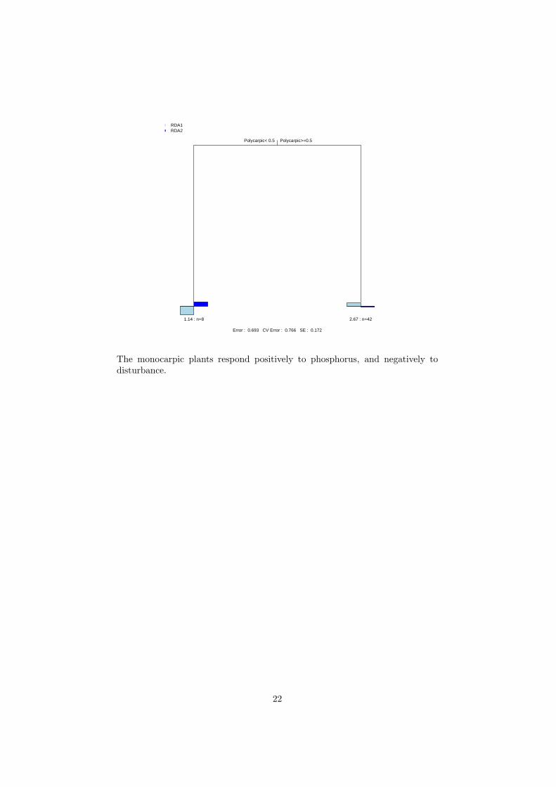
Polycarpic< 0.5 Polycarpic>=0.5

1.14 : n=8 2.67 : n=42

RDA1RDA2

Error : 0.693 CV Error : 0.766 SE : 0.172

The monocarpic plants respond positively to phosphorus, and negatively todisturbance.

22

6 E-”OMI-GAM”: outlying mean index and gen-eralised additive model


The Outlying Mean Index (OMI) is a multivariate method to separate speciesniches and to measure the distance between the mean habitat conditions usedby each species and the mean habitat conditions of the study area (Doledecet al., 2000; Thuiller et al., 2004). OMI-GAM starts by determining the speciesresponse to the environmental gradients (component 1) and models the con-tribution of each trait to the response (component 2). Finally, it clusters thespecies according to the responsive species - trait models (component 3).

� Step 1: Component 1 (species responses to environmental variables)

The Outlying Mean Index makes no assumption about the shape of speciesresponse curves to the environment (e.g. unimodal or linear) and, unlikeCCA and RDA, gives equal weight to species-rich and species-poor sites.The result of this analysis describes the mean position of the species in theenvironmental space (along each environmental axis), which represents ameasure of the distance between the mean habitat conditions used by thespecies and the mean habitat conditions of the study area. It measuresthe propensity of the species to select a specialized environment.

� Step 2: Component 2 (identification of responsive trait combinations)

They are various techniques to analysis the relationship between species’niche position and selected functional traits (e.g. regression-type, classification-type). Here we used inference-based generalized additive models. Stepwiseregression-backward, forward or both–is an obvious method for examiningthe relative importance of each functional trait to explain species nicheposition on the selected axes. However, using usual stepwise regressionto find the optimal combination of explanatory variables to model a re-sponse is often considered to be a high-variance operation because smallperturbations of the response data can sometimes lead to vastly differentsubsets of the variables (Johnson and Omland, 2004). To avoid this prob-lem, and to measure the actual power of each functional trait we usedmultimodal inference based on all-subsets selection of generalised addi-tive models (Burnham and Anderson, 2002; Thuiller et al., 2007). In thecase of six functional traits, there are 26 = 64 possible models in an all-subsets selection. We thus estimated a small-sample (second order) biasadjustment of AIC (AICc) for each submodel. To estimate the weight ofevidence of each functional trait (wpi) to explain species niche positionon each OMI axis, we simply summed the model AICs weights (wi) overall models in which predictor appeared. To derive predicted species nicheposition, we averaged the predictions from each submodel weighted by themodel AICc weight (see also method 2). This procedure was carried outfor the two selected OMI axes.

� Step 3: Component 3 (grouping of species based on responsive traits)

Outputs of inference-based GAM were used to define functional groups.Euclidean distances between species were computed on the predictions

23

from inference-based GAM over the selected axes of OMI analysis andWard’s hiercharchical clustering was then performed. Clusters were ex-tracted from the dendrogram and the optimal number of functional groupswas determined with the Calinsky-Harabasz stopping criterion. Correla-tion ratios were computed to measure the degree of correlation betweenspecies traits and response groups.

6.2 Results

6.2.1 Analysis of environment

Prior to OMI analysis, environmental data must be analysed. Here, we use aPCA on correlation matrix:

> pca.env<-dudi.pca(env, scannf=FALSE)> scatter(pca.env)

d = 1

GE−MNP_1

GE−MNP_10

GE−MNP_11 GE−MNP_12

GE−MNP_13 GE−MNP_14 GE−MNP_15

GE−MNP_17

GE−MNP_18


GE−MNP_20

GE−MNP_21

GE−MNP_22


GE−MNP_25


GE−MNP_29

GE−MNP_3

GE−MNP_31

GE−MNP_33 GE−MNP_34 GE−MNP_35 GE−MNP_36



GE−MNP_40


GE−MNP_43


GE−MNP_47

GE−MNP_48

GE−MNP_5

GE−MNP_6

GE−MNP_7

GE−MNP_8

GE−MNP_9

dist.int

SOIL.P

SOIL.WHC

Eigenvalues

The total variation is decomposed onto othogonal axes. The percentage ofvariation associated to each axis:

> 100 * pca.env$eig/sum(pca.env$eig)

[1] 50.86 33.28 15.85

The correlations between environmental variables and PCA axes:> pca.env$co

Comp1 Comp2dist.int 0.87264 0.02217SOIL.P -0.07431 0.99704SOIL.WHC 0.87113 0.06285

24

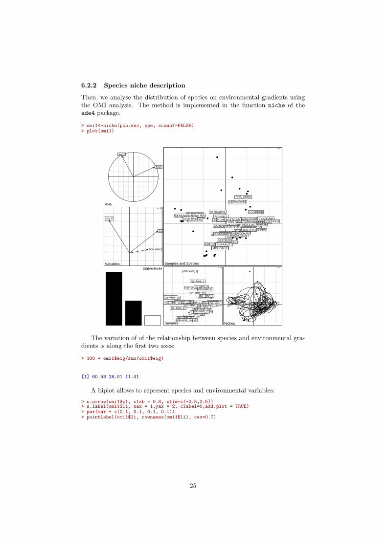
6.2.2 Species niche description

Then, we analyse the distribution of species on environmental gradients usingthe OMI analysis. The method is implemented in the function niche of theade4 package.

> omi1<-niche(pca.env, spe, scannf=FALSE)> plot(omi1)

x1

Axis1

Axis2

Axis d = 0.2

Variables

d = 0.2

dist.int

SOIL.P

SOIL.WHC

Variables Eigenvalues

d = 1

Samples and Species

●

●

●

●

●●

●

● ●

●

●

●

●

●

●●

●

●●

●

●

●

● ●

●

●

●●

●

●

●

●●

●

●●

●

●

●

●

●

●

●

ACHIMILL AGROCAPI

ANTHODOR

BRIZMEDI

BROMHORD

CAPSBURS

CAREFLAC

CAREHIRT

CARENIGR

CENTJACE

CERAARVE

CERAGLOM

CIRSARVE

CYNOCRIS DAUCCARO

DESCCESP.CES

EQUIPALU

FESTOVIN

FESTPRAT

FESTRUBR

GALIMOLL

GALIULIG

HIERACIU

HOLCLANA

HYDRVULG

LEONAUTU

LOLIPERE

LOTUULIG

LUZUCAMP

MATRMARI.INO

MOLICAER PHRAAUST

PLANLANC

POA_ANNU

POTEANSE

POTEEREC

POTEREPT

RANUACRI RANUREPE

RUBUIDAE

RUMEACETOSEL SENEJACO

STELGRAM

TRIFARVE

TRIFPRAT TRIFREPE

VEROARVE

VEROCHAM

VICICRAC

VIOLTRIC

d = 1

Samples

GE−MNP_1

GE−MNP_10


GE−MNP_15


GE−MNP_19

GE−MNP_2

GE−MNP_20



GE−MNP_25


GE−MNP_29

GE−MNP_3

GE−MNP_31



GE−MNP_39

GE−MNP_4

GE−MNP_40

GE−MNP_41 GE−MNP_42 GE−MNP_43 GE−MNP_44 GE−MNP_45

GE−MNP_47

GE−MNP_48

GE−MNP_5

GE−MNP_6

GE−MNP_7

GE−MNP_8

GE−MNP_9

d = 1

Niches

●

●

●

●

●●

●

● ●

●

●

●

●

●

●●

●

●●

●

●

●

● ●

●

●

●●

●

●

●

●●

●

●●

●

●

●

●

●

●

●

The variation of of the relationship between species and environmental gra-dients is along the first two axes:

> 100 * omi1$eig/sum(omi1$eig)

[1] 60.58 28.01 11.41

A biplot allows to represent species and environmental variables:

> s.arrow(omi1$c1, clab = 0.8, xlim=c(-2.5,2.5))> s.label(omi1$li, xax = 1,yax = 2, clabel=0,add.plot = TRUE)> par(mar = c(0.1, 0.1, 0.1, 0.1))> pointLabel(omi1$li, rownames(omi1$li), cex=0.7)

25

d = 1 d = 1

dist.int

SOIL.P

SOIL.WHC

●

●

●

●

●

●

●

●

●

●

●

●

●

●

●

●

●

●

●

●

●

●

●

●

●

●

●

●

●

●

●

●

●

●

●

●

●

●

●

●

●

●

●

●

●

●

●

●

●

● ACHIMILL

AGROCAPI

ANTHODOR

BRIZMEDI

BROMHORD

CAPSBURS

CAREFLAC

CAREHIRT

CARENIGR

CENTJACE

CERAARVE

CERAGLOM

CIRSARVE

CYNOCRIS

DAUCCARO

DESCCESP.CES

EQUIPALUFESTOVIN

FESTPRAT

FESTRUBR

GALIMOLL

GALIULIG

HIERACIU

HOLCLANA

HYDRVULG

LEONAUTU

LOLIPERE

LOTUULIG

LUZUCAMP

MATRMARI.INO

MOLICAER

PHRAAUST

PLANLANC

POA_ANNU

POTEANSE

POTEEREC

POTEREPT

RANUACRI

RANUREPE

RUBUIDAE

RUMEACETOSEL

SENEJACO

STELGRAM

TRIFARVE

TRIFPRAT

TRIFREPE

VEROARVE

VEROCHAM

VICICRAC

VIOLTRIC

The first axis is strongly positively linked to intensity of disturbance and to soilwater holding capacity. The second axis is positively related to soil phosphorous.

Niche position and niche breadth on the first two axes of OMI analysis canbe represented using the sco.distri function:

> par(mfrow=c(1,2))> sco.distri(omi1$ls[,1],spe,clab=0.7)> sco.distri(omi1$ls[,2],spe,clab=0.7)

d = 1

ACHIMILL●AGROCAPI●

ANTHODOR●

BRIZMEDI●

BROMHORD ●

CAPSBURS●

CAREFLAC ●

CAREHIRT●

CARENIGR●

CENTJACE ●

CERAARVE ●

CERAGLOM●

CIRSARVE ●

CYNOCRIS ●DAUCCARO●

DESCCESP.CES ●

EQUIPALU ●

FESTOVIN ●

FESTPRAT ●

FESTRUBR ●

GALIMOLL ●

GALIULIG ●

HIERACIU●

HOLCLANA ●

HYDRVULG●

LEONAUTU ●

LOLIPERE ●

LOTUULIG●

LUZUCAMP ●

MATRMARI.INO●

MOLICAER●

PHRAAUST ●

PLANLANC ●POA_ANNU ●

POTEANSE●

POTEEREC●

POTEREPT ●

RANUACRI ●

RANUREPE ●

RUBUIDAE ●RUMEACETOSEL ●

SENEJACO●

STELGRAM ●

TRIFARVE●

TRIFPRAT ●

TRIFREPE ●

VEROARVE●

VEROCHAM ●

VICICRAC ●

VIOLTRIC●

d = 1

ACHIMILL●

AGROCAPI●

ANTHODOR●

BRIZMEDI●

BROMHORD ●

CAPSBURS●

CAREFLAC●

CAREHIRT●

CARENIGR●

CENTJACE●

CERAARVE ●

CERAGLOM●

CIRSARVE●

CYNOCRIS●

DAUCCARO●

DESCCESP.CES●

EQUIPALU●FESTOVIN●

FESTPRAT●

FESTRUBR●

GALIMOLL●

GALIULIG●

HIERACIU●

HOLCLANA●

HYDRVULG●

LEONAUTU●

LOLIPERE●

LOTUULIG●

LUZUCAMP●

MATRMARI.INO●

MOLICAER●

PHRAAUST●

PLANLANC●

POA_ANNU ●

POTEANSE●

POTEEREC●

POTEREPT●

RANUACRI●

RANUREPE●

RUBUIDAE●

RUMEACETOSEL●

SENEJACO●

STELGRAM●

TRIFARVE●

TRIFPRAT●

TRIFREPE●

VEROARVE●

VEROCHAM●

VICICRAC●

VIOLTRIC●

The niche position of each species (contained in omi1$li) are then extracted foreach axis (species scores) and used as response variable into the inference-basedGAM with functional traits as explanatory variables.

26

6.2.3 Inference based model - GAM

The generalised additive models will relate the mean position of species on OMIaxes to species traits. The list of the 63 possible models (all possible modelsexcept the one which contains only the intercept) is created by the functionInference_modelset. Then, AICc and related measures corresponding to eachmodel, are obtained by the Inference_compute function. Here, the ’Polycarpic’trait is coded as a factor (for a convenient GAM modelling).

> traits[,1]<-as.factor(traits[,1])> modelset<-Inference_modelset(Explanatory=traits)> inf.axis1 <- Inference_compute(Fam="gaussian", combin=modelset[[1]], Mat=modelset[[2]],

Response=omi1$li[,1], Explanatory=traits, Average = TRUE)> inf.axis2 <- Inference_compute(Fam="gaussian", combin=modelset[[1]], Mat=modelset[[2]],

Response=omi1$li[,2], Explanatory=traits, Average = TRUE)

Variable importances from the inference based model (Figure 4a of the pa-per):

> dd.names <- c('Poly- carpic','CN ratio', 'Log(SM)','Height','Onset flowering', 'SLA')

> dd.names.2 <- sapply(dd.names, function(x) gsub("\\s", "\\\n", x))> barplot(inf.axis1$Var.importance[,1], names.arg=dd.names.2)

Poly−carpic

CNratio Log(SM) Height

Onsetflowering SLA

0.0

0.2

0.4

0.6

0.8

Along the OMI axis 1 (intensity of disturbance – soil water holding capac-ity), the GAM inference-based approach together with the permutation testexpressed C:N-ratio and flowering mode (polycarpic vs. monocarpic) as rela-tively important.

Response curves for the OMI axis 1 are then plotted for each trait (Figure4b in the paper).

27

> Limits <- apply(inf.axis1$Plot.response[, seq(2, 12, by=2)], 2, range)> lim <- c(min(Limits[1,]), max(Limits[2,]))> par(mfrow=c(3,2))> plot(as.factor(inf.axis1$Plot.response[,1]), inf.axis1$Plot.response[,2],

ylim=lim, type="l", xlab="Policarpic", ylab="Species position axis 1")> plot(inf.axis1$Plot.response[,3], inf.axis1$Plot.response[,4], ylim=lim,

type="l", xlab="CN ratio", ylab="Species position on OMI axis 1")> plot(inf.axis1$Plot.response[,5], inf.axis1$Plot.response[,6], ylim=lim,

type="l", xlab="Log (Seed mass)", ylab="Species position on OMI axis 1")> plot(inf.axis1$Plot.response[,9], inf.axis1$Plot.response[,10], ylim=lim,

type="l", xlab="Height", ylab="Species position on OMI axis 1")> plot(inf.axis1$Plot.response[,11], inf.axis1$Plot.response[,12], ylim=lim,

type="l", xlab="Onset of flowering", ylab="Species position on OMI axis 1")> plot(inf.axis1$Plot.response[,7], inf.axis1$Plot.response[,8], ylim=lim,

type="l", xlab="SLA", ylab="Species position on OMI axis 1")

0 1

−1.

00.

01.

0

Policarpic

Spe

cies

pos

ition

axi

s 1

10 15 20 25 30 35 40

−1.

00.

01.

0

CN ratio

Spe

cies

pos

ition

on

OM

I axi

s 1

−3 −2 −1 0 1

−1.

00.

01.

0

Log (Seed mass)

Spe

cies

pos

ition

on

OM

I axi

s 1

10 20 30 40 50 60

−1.

00.

01.

0

Height

Spe

cies

pos

ition

on

OM

I axi

s 1

100 120 140 160 180 200

−1.

00.

01.

0

Onset of flowering

Spe

cies

pos

ition

on

OM

I axi

s 1

10 20 30 40

−1.

00.

01.

0

SLA

Spe

cies

pos

ition

on

OM

I axi

s 1

In summary, species on intensely disturbed sites with high soil water holdingcapacity tend to be polycarpic, and to have lower CN ratio than species occur-ring in less intense disturbed places. Along the second axis (soil phosphorousgradient, not shown in the paper and the tutorial), flowering mode, CN ratioare again the most correlated to species position, followed by onset of flowering.Monocarpic species tend to be preferably on sites with high soil phosphorouscontent, with high CN ratio and early onset of flowering than species occurringon lower soil phosphorous content.

We perform the classification using these scores to obtain functional groups:

> Averaged.Pred.1.2<-cbind(inf.axis1$Averaged.Pred, inf.axis2$Averaged.Pred)> hc1 <- hclust(dist(Averaged.Pred.1.2), method = "ward")> plot(hc1)

28

PO

A_A

NN

UC

ER

AG

LOM

MA

TR

MA

RI.I

NO

VE

RO

AR

VE

VIO

LTR

ICB

RO

MH

OR

DC

AP

SB

UR

ST

RIF

AR

VE

AC

HIM

ILL

CA

RE

HIR

TP

OT

EA

NS

EA

NT

HO

DO

RP

OT

ER

EP

TG

ALI

MO

LLR

AN

UR

EP

ET

RIF

PR

AT

LOT

UU

LIG

RU

ME

AC

ET

OS

EL

CE

RA

AR

VE

LUZ

UC

AM

PF

ES

TP

RA

TD

AU

CC

AR

OLO

LIP

ER

EV

ICIC

RA

CR

AN

UA

CR

IT

RIF

RE

PE

CA

RE

FLA

CF

ES

TO

VIN

RU

BU

IDA

EG

ALI

ULI

GC

AR

EN

IGR

MO

LIC

AE

RB

RIZ

ME

DI

PO

TE

ER

EC

SE

NE

JAC

OC

IRS

AR

VE

DE

SC

CE

SP

.CE

SF

ES

TR

UB

RH

IER

AC

IUP

LAN

LAN

CV

ER

OC

HA

MH

YD

RV

ULG

HO

LCLA

NA

CY

NO

CR

ISS

TE

LGR

AM

AG

RO

CA

PI

EQ

UIP

ALU

PH

RA

AU

ST

CE

NT

JAC

ELE

ON

AU

TU

05

1015

Cluster Dendrogram

hclust (*, "ward")dist(Averaged.Pred.1.2)

Hei

ght

We use the Calinsky-Harabasz criteria to find the best partition (try between2 and 6 groups).

> ntest <- 6> res <- rep(0,ntest - 1)> for (i in 2:ntest){

fac <- cutree(hc1, k = i)res[i-1] <- calinski(tab=Averaged.Pred.1.2, fac = fac)[1]

}> par(mfrow=c(1,2))> plot(2:ntest, res, type='b', pch=20, xlab="Number of groups", ylab = "C-H index")> plot(3:ntest, diff(res), type='b', pch=20, xlab="Number of groups", ylab = "Diff in C-H index")

29

●

●

●

●

●

2 3 4 5 6

8010

012

014

016

0

Number of groups

C−

H in

dex

●

●

●

●

3.0 4.0 5.0 6.0

010

2030

40Number of groups

Diff

in C

−H

inde

x

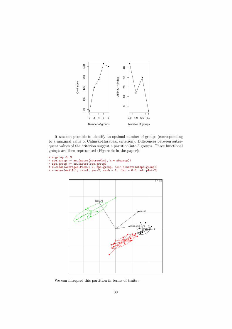
It was not possible to identify an optimal number of groups (correspondingto a maximal value of Calinski-Harabasz criterion). Differences between subse-quent values of the criterion suggest a partition into 3 groups. Three functionalgroups are then represented (Figure 4c in the paper):

> nbgroup <- 3> spe.group <- as.factor(cutree(hc1, k = nbgroup))> spe.group <- as.factor(spe.group)> s.class(Averaged.Pred.1.2, spe.group, col= 1:nlevels(spe.group))> s.arrow(omi1$c1, xax=1, yax=2, csub = 1, clab = 0.8, add.plot=T)

d = 0.5

●●

●

●

●

●

●●

●

●

●●

●

●

●

●

● ●

●

●

●

●

●

●

●

●

●

●

●●

●

●

●

●

●

●●

●

●

●

●

●

●

●

●

●

●

●

●

●

1

2

3 dist.int

SOIL.P

SOIL.WHC

We can interpret this partition in terms of traits :

30

> eta2 <- cor.ratio(traits[,-1], data.frame(spe.group), weights = rep(1, length(spe.group)))> par(mfrow=n2mfrow(ncol(traits)))> plot(table(spe.group,traits[,1]), main =names(traits)[1])> for(i in 2:ncol(traits)){

label <- paste(names(traits)[i], "(cor.ratio =", round(eta2[i-1],3), ")")plot(traits[,i]~spe.group, main = label, border = 1:nlevels(spe.group))

}

Polycarpic

spe.group

1 2 301

1 2 3

1020

3040

Cnratio (cor.ratio = 0.639 )

spe.grouptr

aits

[, i]

●

●

●

1 2 3

−3

−2

−1

01

seed.mass.log (cor.ratio = 0.294 )

spe.group

trai

ts[,

i]

1 2 3

1020

3040

SLA (cor.ratio = 0.32 )

spe.group

trai

ts[,

i]

●

1 2 3

1030

50

height (cor.ratio = 0.381 )

spe.group

trai

ts[,

i]

●

●

●

1 2 3

100

140

180

Onset.flower (cor.ratio = 0.491 )

spe.group

trai

ts[,

i]

The first group contains 18 polycarpic species with a low CN ratio, occurringin very disturbed sites, with a high soil water holding capacity and medium soilphosphorous content. The second group comprises 24 polycarpic species witha higher CN ratio than group 1 and 3, later onset of flowering that the othergroups, and occurring mostly in slightly disturbed sites and soil water content,but a low soil phosphorous content. The third group contains only monocarpicspecies, which have intermediate CN ratio compared to the other groups anda large variance for onset of flowering. These species mostly occur in site withhigh soil phosphorous and low intensity of disturbance and soil water content.

The ’Polycarpic’ trait is then retransformed into a binary variable:

> traits[,1]=as.numeric(traits[,1])

31

7 F-”RLQ”: RLQ Analysis


RLQ analysis (Doledec et al., 1996) is a three-table ordination method thatallows the simultaneous analysis of tables R, L and Q in order to summarizeand represent graphically the main patterns of co-variation between trait dataand environmental parameters (components 1, 2). A subsequent cluster analysisbased on the co-variation then produces functional groups (component 3).

� Step 1, 2: Component 1, 2 (species responses to environmental variablesand identification of responsive trait combinations)

RLQ analysis is an extension of the two-table method of co-inertia analysis(Doledec and Chessel, 1994; Dray et al., 2003). It aims at finding a sitescore (linear combination of environmental variables) and a species score(linear combination of traits) maximizing the co-inertia criterion. Thiscriterion is the product of the variance of the site scores by the variance ofthe species scores and by the squared cross-correlation between the speciesscore and the sites score mediated by table L.


Outputs of RLQ analysis were used to define functional groups. Eu-clidean distances between species were computed on the first two axes ofRLQ analysis and Ward’s hiercharchical clustering was then performed.Clusters were extracted from the dendrogram and the optimal number offunctional groups was determined with the Calinsky-Harabasz stoppingcriterion. Correlation ratios were computed to measure the degree of cor-relation between species traits and response groups.

7.2 Results

Prior to the analysis, the table L must be analysed by correspondence analy-sis. Species and sites weights computed in these analysis are then used in theanalyses of species traits (Q) and environmental variables (R).

> pca.traits <- dudi.pca(traits, row.w = coa1$cw, scannf = FALSE)> pca.env <- dudi.pca(env, row.w = coa1$lw, scannf = FALSE)

The RLQ analysis is performed using the rlq function of the ade4 package:

> rlq1 <- rlq(pca.env, coa1, pca.traits, scannf = FALSE)> summary(rlq1)

Eigenvalues decomposition:eig covar sdR sdQ corr

1 0.3474 0.5894 0.9994 1.317 0.44792 0.2530 0.5030 1.1860 1.136 0.3732

Inertia & coinertia R:inertia max ratio

1 0.9989 1.581 0.631612 2.4054 2.553 0.9423

Inertia & coinertia Q:inertia max ratio

1 1.734 2.223 0.780012 3.025 3.195 0.9467

32

Correlation L:corr max ratio

1 0.4479 0.8483 0.52802 0.3732 0.8160 0.4574

The main outputs of the analysis can be represented:

> plot(rlq1)

d = 1

R row scores


GE−MNP_11



GE−MNP_17

GE−MNP_18

GE−MNP_19

GE−MNP_2

GE−MNP_20

GE−MNP_21


GE−MNP_25


GE−MNP_29

GE−MNP_3

GE−MNP_31


GE−MNP_35


GE−MNP_39

GE−MNP_4

GE−MNP_40




GE−MNP_7

GE−MNP_8

GE−MNP_9

d = 2

Q row scores

ACHIMILL AGROCAPI

ANTHODOR

BRIZMEDI

BROMHORD

CAPSBURS

CAREFLAC

CAREHIRT

CARENIGR

CENTJACE

CERAARVE

CERAGLOM CIRSARVE

CYNOCRIS

DAUCCARO

DESCCESP.CES

EQUIPALU

FESTOVIN

FESTPRAT

FESTRUBR

GALIMOLL

GALIULIG

HIERACIU HOLCLANA HYDRVULG

LEONAUTU

LOLIPERE

LOTUULIG

LUZUCAMP

MATRMARI.INO

MOLICAER

PHRAAUST

PLANLANC

POA_ANNU

POTEANSE

POTEEREC

POTEREPT

RANUACRI RANUREPE

RUBUIDAE

RUMEACETOSEL

SENEJACO

STELGRAM

TRIFARVE

TRIFPRAT

TRIFREPE VEROARVE

VEROCHAM

VICICRAC

VIOLTRIC

x1

Ax1

Ax2

R axes

d = 0.2

R Canonical weights

d = 0.2

dist.int

SOIL.P

SOIL.WHC

R Canonical weights

x1

Ax1 Ax2

Q axes

d = 0.2

Q Canonical weights

d = 0.2 Polycarpic

Cnratio

seed.mass.log SLA

height

Onset.flower Q Canonical weights

Eigenvalues

The co-structure between traits and environment is mainly decomposed ontothe two first axes of RLQ analysis (57.18 % and 41.64 % of the co-inertia criterionfor the first and second RLQ axis respectively):

> ## Percentage of co-Inertia for each axis> 100*rlq1$eig/sum(rlq1$eig)

[1] 57.178 41.642 1.180

To interpret the results, correlations can be computed:

> ## weighted correlations axes / env.> t(pca.env$tab)%*%(diag(pca.env$lw))%*%as.matrix(rlq1$mR)

33

NorS1 NorS2dist.int 0.09551 0.9600SOIL.P -0.99445 -0.1151SOIL.WHC 0.17425 0.7638

> ## weighted correlations axes / traits.> t(pca.traits$tab)%*%(diag(pca.traits$lw))%*%as.matrix(rlq1$mQ)

NorS1 NorS2Polycarpic 0.7171 0.1551Cnratio 0.5583 -0.6262seed.mass.log 0.4932 0.1148SLA -0.6396 0.6372height 0.5221 -0.3725Onset.flower 0.4782 -0.7687

> ## correlations traits / env.> rlq1$tab

Polycarpic Cnratio seed.mass.log SLA heightdist.int 0.1468 -0.2183 0.13662 0.17193 -0.08406SOIL.P -0.4312 -0.1729 -0.25391 0.16159 -0.11785SOIL.WHC 0.1244 -0.1153 0.09662 0.05833 0.05672

Onset.flowerdist.int -0.30212SOIL.P -0.14185SOIL.WHC -0.08219

The first axis is negatively correlated to soil phosophate. It is also negativelyrelated to SLA and positively to all other traits. The second axis is positivelycorrelated to disturbance frequency and soil water content. It is positively re-lated to SLA and negatively to Onset of flowering, C:N ratio.

A biplot representing traits and environmental variables (Figure 3c in thepaper) can be constructed:

> s.arrow(rlq1$c1, xlim=c(-1,1), boxes = FALSE)> s.label(rlq1$li, add.plot=T, clab=1.5)

d = 0.5 d = 0.5

Polycarpic

Cnratio

seed.mass.log SLA

height

Onset.flower

dist.int

SOIL.P

SOIL.WHC

Species scores on the first two axes of RLQ analysis:

34

> s.label(rlq1$lQ, clabel = 0)> par(mar = c(0.1, 0.1, 0.1, 0.1))> pointLabel(rlq1$lQ,row.names(rlq1$lQ), cex=0.7)

d = 2

●

●

●

●

●

●

●

●

●

●

●

●

●

●

●

●

●

●

●

●

●

●

●

●●

●

●

●

●

●

●

●

●

●

●

●

●

●

●

●

●

●

●

●

●

●●

●

●

●

ACHIMILL

AGROCAPI

ANTHODOR

BRIZMEDI

BROMHORD

CAPSBURS

CAREFLAC

CAREHIRT

CARENIGR

CENTJACE

CERAARVE

CERAGLOMCIRSARVE

CYNOCRIS

DAUCCARO

DESCCESP.CES

EQUIPALU

FESTOVIN

FESTPRAT

FESTRUBR

GALIMOLL

GALIULIG

HIERACIU

HOLCLANAHYDRVULG

LEONAUTU

LOLIPERE

LOTUULIG

LUZUCAMP

MATRMARI.INO

MOLICAER

PHRAAUST

PLANLANC

POA_ANNU

POTEANSE

POTEEREC

POTEREPT

RANUACRI

RANUREPE

RUBUIDAE

RUMEACETOSEL

SENEJACO

STELGRAM

TRIFARVE

TRIFPRAT

TRIFREPEVEROARVE

VEROCHAM

VICICRAC

VIOLTRIC

We perform the classification using these scores to obtain functional groups:

> hc2 <- hclust(dist(rlq1$lQ), method = "ward")> plot(hc2)

35

CIR

SA

RV

ER

UB

UID

AE

CA

RE

FLA

CM

OLI

CA

ER

PH

RA

AU

ST

CA

RE

NIG

RF

ES

TO

VIN

DE

SC

CE

SP

.CE

SS

EN

EJA

CO

BR

IZM

ED

IP

OT

EE

RE

CC

EN

TJA

CE

FE

ST

RU

BR

PLA

NLA

NC

BR

OM

HO

RD

AG

RO

CA

PI

TR

IFA

RV

EC

YN

OC

RIS

HIE

RA

CIU

PO

TE

AN

SE

GA

LIU

LIG

LEO

NA

UT

UA

CH

IMIL

LV

ER

OC

HA

MV

ICIC

RA

CG

ALI

MO

LLR

AN

UR

EP

ET

RIF

PR

AT

CA

RE

HIR

TF

ES

TP

RA

TH

OLC

LAN

ALO

TU

ULI

GLO

LIP

ER

ED

AU

CC

AR

OR

AN

UA

CR

IP

OT

ER

EP

TS

TE

LGR

AM

TR

IFR

EP

ER

UM

EA

CE

TO

SE

LA

NT

HO

DO

RH

YD

RV

ULG

EQ

UIP

ALU

CE

RA

GLO

MC

AP

SB

UR

SM

AT

RM

AR

I.IN

OC

ER

AA

RV

ELU

ZU

CA

MP

PO

A_A

NN

UV

ER

OA

RV

EV

IOLT

RIC

05

1015

2025

30

Cluster Dendrogram

hclust (*, "ward")dist(rlq1$lQ)

Hei

ght

We use the Calinsky-Harabasz criteria to find the best partition (try between2 and 6 groups) :> ntest <- 6> res <- rep(0,ntest - 1)> for (i in 2:ntest){

fac <- cutree(hc2, k = i)res[i-1] <- calinski(tab=rlq1$lQ, fac = fac)[1]


●

●

●

●

●

2 3 4 5 6

3540

4550

Number of groups

C−

H in

dex

●

●

●

●

3.0 4.0 5.0 6.0

−5

05

1015

Number of groups

Diff

in C

−H

inde

x

36

The best partition is for 4 groups. In the next figure, each point representsthe modelled species position on RLQ axes 1 and 2 , and each colour the groupfrom the cluster:

> spe.group2 <- as.factor(cutree(hc2, k = which.max(res) +1))> levels(spe.group2) <- c("C","B","D","A")> spe.group2 <- factor(spe.group2, levels=c("A","B","C","D"))> s.class(rlq1$lQ, spe.group2, col= 1:nlevels(spe.group2))> s.arrow(rlq1$c1, add.plot = T,clab=0.8)

d = 2

●

●

●

●

●

●

●

●

●

●

●●

●

●

●

●

●

●●

●

●

●

●

●

●

●

●

●

●

●

●●

●

●

●

●

●

●

●●

●

●

●

●

●

●

●

●

●

●

A

B

C

D

Polycarpic

Cnratio

seed.mass.log SLA

height

Onset.flower


> eta2 <- cor.ratio(traits[,-1], data.frame(spe.group2), weights = rep(1, length(spe.group2)))> par(mfrow=n2mfrow(ncol(traits)))> plot(table(spe.group2,traits[,1]), main =names(traits)[1])> for(i in 2:ncol(traits)){

label <- paste(names(traits)[i], "(cor.ratio =", round(eta2[i-1],3), ")")plot(traits[,i]~spe.group2, main = label, border = 1:nlevels(spe.group2))

}

37

Polycarpic

spe.group2

A B C D1

2

●

●

●

A B C D

1020

3040


spe.group2

trai

ts[,

i]

A B C D

−3

−2

−1

01


spe.group2

trai

ts[,

i]

A B C D

1020

3040


spe.group2

trai

ts[,

i]

●

●

A B C D

1030

50


spe.group2

trai

ts[,

i]

●

●

A B C D

100

140

180


spe.group2

trai

ts[,

i]

A first group (A) contains 5 species with very low value of Onset of flower-ing, low height and high SLA. These species occupied mainly highly disturbedenvironment with high phosphate. A second group (B) of 14 polycarpic speciesis identified. These species have very high C:N ratio, high height, low SLA andhigh value of Onset of flowering and they occupied sites with low phosphateand moderate disturbance intensity. A third intermediate group (C) contains27 species which are mainly polycarpic (25 species), with quite high SLA. Thesespecies occupied mainly highly disturbed environment with low phosphate. Thefourth group (D) with 4 species including 3 monocarpic corresponds to specieswith high value of of Onset of flowering, low seed mass and low SLA that occu-pied sites with high phosphate and low disturbance intensity.

The classification obtained is quite similar to the one obtained with OMI-GAM:> table(spe.group,spe.group2)

spe.group2spe.group A B C D

1 2 0 16 02 0 14 9 13 3 0 2 3

The only difference is that RLQ has an additional group which corresponds tothe splitting of a group of 24 species into two groups of 15 and 9 species.

38

8 G-”Double CCA”: double canonical correspon-dence analysis


� Step 1, 2: Component 1, 2 (species responses to environmental variablesand identification of responsive trait combinations)

Double CCA is a three-table ordination method proposed by Lavorel et al.(1999, 1998). In the classical context, canonical correspondence analysis(CCA) is used to link tables L and R in order to ordinate the communitydata in the light of the environmental variables. It is well known that CCAimplies two main steps: (1) prediction of community data by environmentand (2) ordination of predicted values. Ojeda et al. (1998) performed anunusual CCA in which the ordination of L is constrained by the speciestraits table Q. Lavorel and coauthors proposed to combine these two CCAin one analysis nicknamed ”double CCA”. This approach ordinates L bytaking the effects of R and Q simultaneously into account. Double CCAencompasses also two steps: (1) prediction of community data by bothenvironmental variables and species traits and (2) ordination of predictedvalues.


As in RLQ, functional groups were defined using Ward’s hiercharchicalclustering with the Calinsky-Harabasz stopping criterion using speciesscores for the first two axes of the double CCA. Correlation ratios werecomputed to measure the degree of correlation between species traits andresponse groups.

8.2 Results

Double CCA is based on the correspondence analysis of the species-by-sitestable. In this analysis, the ordination of sites and species is constrained by bothspecies traits and environment:

> dbcca1 <- dbrda(coa1,env, traits, scannf = FALSE)

For the double CCA, the three environmental variables and the six traitsexplain 6.25 % of the variation (14.89 % for the environment in standard CCA).

> ## percentage of explained variation by the environment> sum(cca1$eig)/sum(coa1$eig)*100

[1] 14.89

> ## percentage of explained variation by both traits and env.> sum(dbcca1$eig)/sum(coa1$eig)*100

[1] 6.248

This explained variation is mainly decomposed onto the first two axes of theanalysis (58.2 % and 38.34 % for the first and second axis respectively):

39

> ## Percentage of variation explained by each axis> 100*dbcca1$eig/sum(dbcca1$eig)

[1] 58.196 38.338 3.466

Correlations between axes and traits and environmental variables (Figure 3cin the paper) can then be used to interpret the results:

> s.arrow(dbcca1$corZ[-1,], xlim=c(-1.2,1.2), boxes = FALSE)> s.label(dbcca1$corX[-1,], add.plot=T, clab=1.5)

d = 0.5 d = 0.5

Polycarpic

Cnratio

seed.mass.log

SLA

height

Onset.flower

dist.int

SOIL.P SOIL.WHC

The first axis is positively correlated to soil phosophate and negatively correlatedto disturbance frequency. It is also negatively to polycarpic life history and seedmass. The second axis is negatively correlated to disturbance frequency andalso to soil phosophate and soil water holding capacity. It is negatively relatedto SLA and positively to Onset of flowering, C:N ratio and height.

Species scores on the first two axes of double CCA:

> s.label(dbcca1$co, clabel = 0)> par(mar = c(0.1, 0.1, 0.1, 0.1))> pointLabel(dbcca1$co,row.names(dbcca1$co), cex=0.7)

40

d = 0.5

●

●

●

●

●

●

●

●

●

●

●

●●

●

●

●●

●

●

●

●

●

●

●

●

●

●

●

●

●

●

●

●

●

●

●

●

●

●

●

●

●

● ●

●

●

●

●

●

●

ACHIMILL

AGROCAPI

ANTHODOR

BRIZMEDI

BROMHORD

CAPSBURS

CAREFLAC

CAREHIRT

CARENIGR

CENTJACE

CERAARVE

CERAGLOMCIRSARVE

CYNOCRIS

DAUCCARO

DESCCESP.CES EQUIPALUFESTOVIN

FESTPRAT

FESTRUBR

GALIMOLL

GALIULIG

HIERACIU

HOLCLANA

HYDRVULG

LEONAUTU

LOLIPERE

LOTUULIG

LUZUCAMP

MATRMARI.INO

MOLICAER

PHRAAUST

PLANLANC

POA_ANNU

POTEANSE

POTEEREC

POTEREPT

RANUACRI

RANUREPE

RUBUIDAE

RUMEACETOSEL

SENEJACO

STELGRAM TRIFARVE

TRIFPRAT

TRIFREPE

VEROARVE

VEROCHAM

VICICRACVIOLTRIC

We perform the classification using these scores to obtain functional groups:> hc3 <- hclust(dist(dbcca1$co), method = "ward")> plot(hc3)

CA

PS

BU

RS

MA

TR

MA

RI.I

NO

CE

RA

GLO

ME

QU

IPA

LUP

OA

_AN

NU

VE

RO

AR

VE

VIO

LTR

ICG

ALI

MO

LLC

ER

AA

RV

ELU

ZU

CA

MP

AN

TH

OD

OR

RU

ME

AC

ET

OS

EL

ST

ELG

RA

MC

YN

OC

RIS

HY

DR

VU

LGH

OLC

LAN

AP

OT

ER

EP

TH

IER

AC

IUP

OT

EA

NS

EV

ICIC

RA

CC

AR

EH

IRT

RA

NU

RE

PE

LOT

UU

LIG

TR

IFR

EP

ET

RIF

PR

AT

DA

UC

CA

RO

FE

ST

PR

AT

LOLI

PE

RE

RA

NU

AC

RI

BR

OM

HO

RD

TR

IFA

RV

ED

ES

CC

ES

P.C

ES

PH

RA

AU

ST

AC

HIM

ILL

AG

RO

CA

PI

CA

RE

FLA

CM

OLI

CA

ER

SE

NE

JAC

OB

RIZ

ME

DI

PO

TE

ER

EC

CA

RE

NIG

RF

ES

TO

VIN

RU

BU

IDA

EC

EN

TJA

CE

PLA

NLA

NC

FE

ST

RU

BR

GA

LIU

LIG

VE

RO

CH

AM

CIR

SA

RV

ELE

ON

AU

TU

02

46

810

Cluster Dendrogram

hclust (*, "ward")dist(dbcca1$co)

Hei

ght

We use the Calinsky-Harabasz criteria to find the best partition (try between2 and 6 groups) :

41

> ntest <- 6> res <- rep(0,ntest - 1)> for (i in 2:ntest){

fac <- cutree(hc3, k = i)res[i-1] <- calinski(tab=dbcca1$co, fac = fac)[1]


●

●

●

●

●

2 3 4 5 6

4045

5055

60

Number of groups

C−

H in

dex

●

●

●

●

3.0 4.0 5.0 6.0

5.0

5.5

6.0

6.5

7.0

7.5

Number of groups

Diff

in C

−H

inde

x

It was not possible to identify an optimal number of groups as the Calinski-Harabasz criterion increases (but never decreases) with the number of groups.Differences between subsequent values were not helpful in this case. The numberof groups was then arbitrary set to 4 (i.e., the number of groups identified forthe RLQ analysis).

> nbgroup <- ifelse((which.max(res) + 1) == ntest, nlevels(spe.group2), which.max(res) + 1)> spe.group3 <- as.factor(cutree(hc3, k = nbgroup))> levels(spe.group3) <- c("B","C","D","A")> spe.group3 <- factor(spe.group3, levels=c("A","B","C","D"))> s.class(dbcca1$co, spe.group3, col = 1:nlevels(spe.group3))> s.arrow(dbcca1$corZ[-1,],add.plot=T,clab=0.8)

42

d = 0.5

●

●

●

●

●

●

●

●

●

●

●

●

●

●●

●

●

●

●

●●

●

●

●

●

●

●

●

●

●

●

●

●

●

●

●

●

●●

●

●

●

●

●

●

●

●

●

●

●

A

B

C

D

Polycarpic

Cnratio

seed.mass.log

SLA

height

Onset.flower


> eta2 <- cor.ratio(traits[,-1], data.frame(spe.group3), weights = rep(1, length(spe.group3)))> par(mfrow=n2mfrow(ncol(traits)))> plot(table(spe.group3,traits[,1]), main =names(traits)[1])> for(i in 2:ncol(traits)){

label <- paste(names(traits)[i], "(cor.ratio =", round(eta2[i-1],3), ")")plot(traits[,i]~spe.group3, main = label, border = 1:nlevels(spe.group3))

}

43

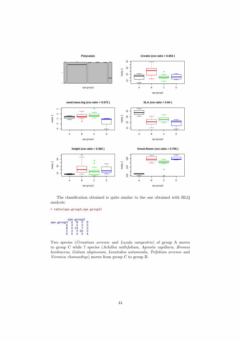
Polycarpic

spe.group3

A B C D1

2

●

A B C D

1020

3040


spe.group3

trai

ts[,

i]●

●

A B C D

−3

−2

−1

01


spe.group3

trai

ts[,

i]

A B C D

1020

3040


spe.group3

trai

ts[,

i]

●

●

●

A B C D

1030

50


spe.group3

trai

ts[,

i]

●

●

●

A B C D

100

140

180


spe.group3

trai

ts[,

i]

The classification obtained is quite similar to the one obtained with RLQanalysis:

> table(spe.group3,spe.group2)

spe.group2spe.group3 A B C D

A 3 0 0 0B 0 14 7 0C 2 0 20 0D 0 0 0 4

Two species (Cerastium arvense and Luzula campestris) of group A movesto group C while 7 species (Achillea millefolium, Agrostis capillaris, Bromushordeaceus, Galium uliginosum, Leontodon autumnalis, Trifolium arvense andVeronica chamaedrys) moves from group C to group B.

44

References

A. Agresti. Categorical data analysis. John Wiley and Sons, 2002.

K. Burnham and D. Anderson. Model selection and multimodel inference. Apractical information-theoretic approach. Springer, 2002.

S. Doledec and D. Chessel. Co-inertia analysis: an alternative method for study-ing species-environment relationships. Freshwater Biology, 31:277–294, 1994.

S. Doledec, D. Chessel, C. ter Braak, and S. Champely. Matching species traitsto environmental variables: a new three-table ordination method. Environ-mental and Ecological Statistics, 3:143–166, 1996.

S. Doledec, D. Chessel, and C. Gimaret-Carpentier. Niche separation in com-munity analysis: a new method. Ecology, 81(10):2914–2927, 2000.

S. Dray, D. Chessel, and J. Thioulouse. Co-inertia analysis and the linking ofecological data tables. Ecology, 84:3078–3089, 2003.

B. Everitt, S. Landau, and M. Leese. Cluster analysis. Arnold, London, 2001.

A. Gordon. Classification. Chapman and Hall, Boca Raton, 1999.

C. Hennig. Cluster-wise assessment of cluster stability. Computational Statisticsand Data Analysis, 52(1):258–271, 2007.

J. Johnson and K. Omland. Model selection in ecology and evolution. Trendsin Ecology & Evolution, 19(2):101–108, 2004.

S. Lavorel, B. Touzard, J. Lebreton, and B. Clement. Identifying functionalgroups for response to disturbance in an abandoned pasture. Acta Oecologica- International Journal of Ecology, 19(3):227–240, 1998.

S. Lavorel, C. Rochette, and J. Lebreton. Functional groups for response todisturbance in Mediterranean old fields. Oikos, 84:480–498, 1999.

P. Legendre and L. Legendre. Numerical Ecology. Elsevier Science, Amsterdam,2nd edition, 1998.

R. Mac Nally. Regression and model-building in conservation biology, biogeog-raphy and ecology: the distinction between–and reconciliation of–‘predictive’and ‘explanatory’ models. Biodiversity and Conservation, 9(5):655–671, 2000.

F. Ojeda, J. Arroyo, and T. Maranon. The phytogeography of European andMediterranean heath species (Ericoideae, Ericaceae): a quantitative analysis.Journal of Biogeography, 25:165–178, 1998.

O. Petchey and K. Gaston. Functional diversity: back to basics and lookingforward. Ecology Letters, 9(6):741–758, 2006.

C. Rao. The use and interpretation of principal component analysis in appliedresearch. Sankhya A, 26:329–359, 1964.

P. Sneath and R. Sokal. Numerical taxonomy: the principles and practice ofnumerical classification. Freeman, San Francisco, 1973.

45

B. Strauss and R. Biedermann. Urban brownfields as temporary habitats: driv-ing forces for the diversity of phytophagous insects. Ecography, 29:928–940,2006.

C. ter Braak. Canonical correspondence analysis: a new eigenvector techniquefor multivariate direct gradient analysis. Ecology, 67:1167–1179, 1986.

W. Thuiller, S. Lavorel, G. Midgley, S. Lavergne, and T. Rebelo. Relating planttraits and species distributions along bioclimatic gradients for 88 Leucaden-dron taxa. Ecology, 85(6):1688–1699, 2004.

W. Thuiller, J. Slingsby, S. Privett, and R. Cowling. Stochastic species turnoverand stable coexistence in a species-rich, fire-prone plant community. PLoSONE, 2:e938, 2007. URL http://dx.plos.org/10.1371%2Fjournal.pone.0000938.

M. Whittingham, P. Stephens, R. Bradbury, and R. Freckleton. Why do we stilluse stepwise modelling in ecology and behaviour? Journal of Animal Ecology,75(5):1182–1189, 2006.

46

Tutorial: Methods for assessing functional responses to ... · PDF fileTutorial: Methods for...

Documents

Transcript of Tutorial: Methods for assessing functional responses to ... · PDF fileTutorial: Methods for...