
Tutorial Math Modeling
54
ÒÉthe very gameÉÓ A Tutorial on Mathematical Modeling Michael P. McLaughlin www.geocities.com/~mikemclaughlin
Transcript of Tutorial Math Modeling

8/14/2019 Tutorial Math Modeling
http://slidepdf.com/reader/full/tutorial-math-modeling 1/54
ÒÉthe very gameÉÓ
A Tutorial on Mathematical Modeling
Michael P. McLaughlinwww.geocities.com/~mikemclaughlin

8/14/2019 Tutorial Math Modeling
http://slidepdf.com/reader/full/tutorial-math-modeling 2/54
ii
© Dr. Michael P. McLaughlin1993-1999
This tutorial is distributed free of charge and may neither be sold nor repackaged for sale inwhole or in part.
Macintosh is a registered trademark of Apple Computer, Inc.

8/14/2019 Tutorial Math Modeling
http://slidepdf.com/reader/full/tutorial-math-modeling 3/54
iii
PREFACE
“OK, I’ve got some data. Now what?”
It is the quintessence of science, engineering, and numerous other disciplines to make
quantitative observations, record them, and then try to make some sense out of the resultingdataset. Quite often, the latter is an easy task, due either to practiced familiarity with thedomain or to the fact that the goals of the exercise are undemanding. However, when workingat the frontiers of knowledge, this is not the case. Here, one encounters unknown territory,with maps that are sometimes poorly defined and always incomplete.
The question posed above is nontrivial; the path from observation to understanding is, ingeneral, long and arduous. There are techniques to facilitate the journey but these are seldomtaught to those who need them most. My own observations, over the past twenty years, havedisclosed that, if a functional relationship is nonlinear, or a probability distribution somethingother than Gaussian, Exponential, or Uniform, then analysts (those who are not statisticians)are usually unable to cope. As a result, approximations are made and reports deliveredcontaining conclusions that are inaccurate and/or misleading.
With scientific papers, there are always peers who are ready and willing to second-guessany published analysis. Unfortunately, there are as well many less mature disciplines whichlack the checks and balances that science has developed over the centuries and which frequentlyaddress areas of public concern. These concerns lead, inevitably, to public decisions andwarrant the best that mathematics and statistics have to offer, indeed, the best that analysts canprovide. Since Nature is seldom linear or Gaussian, such analyses often fail to live up toexpectations.
The present tutorial is intended to provide an introduction to the correct analysis of data. It
addresses, in an elementary way, those ideas that are important to the effort of distinguishinginformation from error. This distinction, unhappily not always acknowledged, constitutes thecentral theme of the material described herein.
Both deterministic modeling (univariate regression) as well as the (stochastic) modeling of random variables are considered, with emphasis on the latter since it usually gets short shrift instandard textbooks. No attempt is made to cover every topic of relevance. Instead, attention isfocussed on elucidating and illustrating core concepts as they apply to empirical data. I am ascientist, not a statistician, and these are my priorities.
This tutorial is taken from the documentation included with the Macintosh software package Regress+ which is copyrighted freeware, downloadable at
http://www.geocities.com/~mikemclaughlin/software/Regress_plus.html
Michael P. McLaughlinMcLean, VAOctober, 1999

8/14/2019 Tutorial Math Modeling
http://slidepdf.com/reader/full/tutorial-math-modeling 4/54
iv
For deeds do die, however nobly done,And thoughts of men do as themselves decay,But wise words taught in numbers for to run,Recorded by the Muses, live for ay.
—E. Spenser [1591]

8/14/2019 Tutorial Math Modeling
http://slidepdf.com/reader/full/tutorial-math-modeling 5/54
“…the very game…”
IS mother was a witch (or so they said). Had she not poisoned the glazier’s wife with
a magic drink and cursed her neighbors’ livestock so that they became mad? Did shenot wander about the town pestering people with her recipes for medicines? Yet, in
spite of such proofs, his filial devotion did not go unrewarded and, with the aid of a goodlawyer plus the support of his friend and patron Rudolph II, Emperor of the Romans, King of Germany, Hungary, Bohemia, &c., Archduke of Austria, &c., the old woman made her finalexit with less flamboyance than some of His Holy Imperial Majesty’s subjects might havewished. However, this is not about the mother but the son—and Mars. Johannes Kepler isremembered, to this day, for his insight and his vision. Even more than his contemporary,Galileo, he is honored not just for what he saw but because he invented a new way of looking.
In astronomy, as in most disciplines, how you look determines what you see and, here,Kepler had a novel approach. He began with data whereas all of his predecessors had begunwith circles. The Aristotelian/Ptolemaic syllogism decreed that perfect motion was circular.Heavenly bodies were perfect. Therefore, they moved in circles, however many it took to saveappearances.
It took a lot. When, more than a quarter of a century before Kepler, Nicolaus Copernicusfinally laid down his compass, he had, quite rightly, placed the Sun in the center of theremaining seven known bodies but he had also increased the number of celestial circles to arecord forty-eight!
Kepler commenced his intellectual journey along the same path. Indeed, in those days, itwas the only path. After many false starts, however, he realized that a collection of circles just
would not work. It was the wrong model; the data demanded something else. Kepler bowedto Nature and, without apology, substituted ellipses for circles. He was the first scientist tosubjugate theory to observation in a way that we would recognize and applaud.
Of course, Kepler was in a unique position. Thanks to Tycho Brahe, he had the best datain the world and he was duly impressed. Still, he could have voted the party line and added yetmore circles. Sooner or later, he would have accumulated enough parameters to satisfy everysignificant figure of every measurement. But it was wrong and it was the wrongness of it thatimpressed Kepler most of all. Although he drew his inspiration from the ancient Pythagoreansand the religious fervor of his own time, his words leave little doubt of his sincerity:
“…Now, as God the maker played,
he taught the game to Naturewhom he created in his image:taught her the very gamewhich he played himself…”
Kepler searched through the data and found the game. He learned the rules and showedthat, if you played well enough, sometimes even emperors take notice. Today, our motivationis different but the game goes on. We begin, of course, with data.
H

8/14/2019 Tutorial Math Modeling
http://slidepdf.com/reader/full/tutorial-math-modeling 6/54
2
DATA
There are two kinds of data: measurements and opinions. This discussion will focusexclusively on the former. In fact, although there are useful exceptions in many disciplines,here we shall discuss only quantitative measurements. Adopting this mild constraint providestwo enormous advantages. The first is the advantage of being able to speak very precisely,
yielding minimal concessions to the vagaries of language. The second is the opportunity toutilize the power of mathematics and, especially, of statistics.
Statistics, albeit a discipline in its own right, is primarily an ever-improving cumulation of mathematical tools for extracting information from data. It is information, not data, that leadsultimately to understanding. Whenever you make measurements, perform experiments, orsimply observe the Universe in action, you are collecting data. However, real data alwaysleave something to be desired. There is an open interval of quality stretching from worthless toperfect and, somewhere in between, will be your numbers, your data. Information, on theother hand, is not permitted the luxury of imperfection. It is necessarily correct, by definition.Data are dirty; information is golden.
To examine data, therefore, is to sift the silt of a riverbed in search of gold. Of course,there might not be any gold but, if there is, it will take some knowledge and considerable skillto find it and separate it from everything else. Not only must you know what gold looks like,but you also have to know what sorts of things masquerade as gold. Whatever the task, youwill need to know the properties of what you seek and what you wish to avoid, the chemistryof gold and not-gold. It is through these properties one can be separated from the other.
An example of real data is shown in Table 1 and Figure 1.1 This dataset consists of valuesfor the duration of daytime (sunrise to sunset) at Boston, Massachusetts over three years. Thefirst day of each month has been tabulated along with the longest and shortest days occurringduring this period. Daytime has been rounded off to the nearest minute.
What can be said about data such as these? It can be safely assumed that they are correct tothe precision indicated. In fact, Kepler’s data, for analogous measurements, were much moreprecise. It is also clear that, at this location, the length of the day varies quite a bit during theyear. This is not what one would observe near the Equator but Boston is a long way fromtropical climes. Figure 1 discloses that daytime is almost perfectly repetitive from year to year,being long in the (Northern hemisphere) Summer and short in the Winter.
Such qualitative remarks, however, are scarcely sufficient. Any dataset as rich as this onedeserves to be further quantified in some way and, moreover, will have to be if the goal is togain some sort of genuine understanding. With scientific data, proof of understanding impliesthe capability to make accurate predictions. Qualitative conclusions are, therefore, inadequate.
Quantitative understanding starts with a set of well-defined metrics. There are several suchmetrics that may be used to summarize/characterize any set of N numbers, y i, such as these
daytime values. The most common is the total-sum-of-squares, TSS, defined in Equation 1.
1 see file Examples:Daytime.in [FAM95]

8/14/2019 Tutorial Math Modeling
http://slidepdf.com/reader/full/tutorial-math-modeling 7/54
3
Table 1. Daytime—Boston, Massachusetts (1995-1997)
Daytime (min.) Day Date
545 1 1 Jan 1995
595 32669 60758 91839 121901 152915 172 21 Jun 1995912 182867 213784 244700 274616 305555 335
540 356 22 Dec 1995544 366 1 Jan 1996595 397671 426760 457840 487902 518915 538 21 Jun 1996912 548865 579782 610
698 640614 671554 701540 721 21 Dec 1996545 732 1 Jan 1997597 763671 791760 822839 852902 883915 903 21 Jun 1997912 913
865 944783 975699 1005615 1036554 1066540 1086 21 Dec 1997545 1097 1 Jan 1998

8/14/2019 Tutorial Math Modeling
http://slidepdf.com/reader/full/tutorial-math-modeling 8/54
4
0 200 400 600 800 1000 1200
Day
500
600
700
800
900
1000
D a y t i m e H m i n L
Figure 1. Raw Daytime Data
Total-sum-of-squares ≡ TSS = y i – y2
Σi = 1
N
1.
where y is the average value of y.
TSS is a positive number summarizing how much the y-values vary about their average(mean). The fact that each x (day) is paired with a unique y (daytime) is completely ignored.By discounting this important relationship, even a very large dataset may be characterized by asingle number, i.e., by a statistic. The average amount of TSS attributable to each point(Equation 2) is known as the variance of the variable, y. Lastly, the square-root of the varianceis the standard deviation, another important statistic.
Variance of y ≡ Var y = 1N
y i – y2
Σi = 1
N
2.
In Figure 1, the y-values come from a continuum but the x-values do not. More often, x isa continuous variable, sampled at points chosen by the observer. For this reason, it is called
the independent variable. The dependent variable, y, describes measurements made at chosenvalues of x and is almost always inaccurate to some degree. Since the x-values are selected inadvance by the observer, they are most often assumed to be known exactly. Obviously, thiscannot be true if x is a real number but, usually, uncertainties in x are negligible compared touncertainties in y. When this is not true, some very subtle complications arise.

8/14/2019 Tutorial Math Modeling
http://slidepdf.com/reader/full/tutorial-math-modeling 9/54
5
Table 2 lists data from a recent astrophysics experiment, with measurement uncertainties
explicitly recorded.2 These data come from observations, made in 1996-1997, of comet Hale-Bopp as it approached the Sun [RAU97]. Here, the independent variable is the distance of thecomet from the Sun. The unit is AU, the average distance (approximately) of the Earth fromthe Sun. The dependent variable is the rate of production of cyanide, CN, a decompositionproduct of hydrogen cyanide, HCN, with units of molecules per second divided by 10 25.
Thus, even when Hale-Bopp was well beyond the orbit of Jupiter (5.2 AU), it was producing
cyanide at a rate of (6 ± 3) x 1025 molecules per second, that is, nearly 2.6 kg/s.
Table 2. Rate of Production of CN in Comet Hale-Bopp
Rate Distance from Sun Uncertainty in Rate(molecules per second)/1025 (AU) (molecules per second)/1025
130 2.9 40190 3.1 70
90 3.3 2060 4.0 2020 4.6 1011 5.0 66 6.8 3
In this example, the uncertainties in the measurements (Table 2, column 3) are a significantfraction of the observations themselves. Establishing the value of the uncertainty for each datapoint and assessing the net effect of uncertainties are crucial steps in any analysis. HadKepler’s data been as poor as the data available to Copernicus, his name would be known onlyto historians.
The data of Table 2 are presented graphically in Figure 2. For each point, the length of theerror bar indicates the uncertainty3 in y. These uncertainties vary considerably and with someregularity. Here, as often happens with observations made by electronic instruments whichmeasure a physical quantity proportional to the target variable, the uncertainty in an observationtends to increase with the magnitude of the observed value.
Qualitatively, these data suggest the hypothesis that the comet produced more and more CNas it got closer to the Sun. This would make sense since all chemical reactions go faster as thetemperature increases. On the other hand, the observed rate at 2.9 AU seems too small. Didthe comet simply start running out of HCN? How likely is it that the rate at 3.1 AU was reallybigger than the rate at 2.9 AU? Are these values correct? Are the uncertainties correct? If theuncertainties are correct, what does this say about the validity of the hypothesis? All of these
are legitimate questions.
2 see file Examples:Hale_Bopp.CN.in
3 In spite of its name, this bar does not indicate error . If it did, the error could be readilyremoved.

8/14/2019 Tutorial Math Modeling
http://slidepdf.com/reader/full/tutorial-math-modeling 10/54
6
2 3 4 5 6 7
Distance HAUL
0
50
100
150
200
250
300
R a t e
Figure 2. Hale-Bopp CN Data
Finally, consider the very “unscientific” data shown in Figure 3. This figure is a plot of thehighest major-league baseball batting averages in the United States, for the years 1901-1997,
as a function of time.4
A player’s batting average is the fraction of his “official at-bats” in which he hit safely.
Thus, it varies continuously from zero to one. It is fairly clear that there is a large differencebetween these data and those shown in Figure 1. The latter look like something from a mathtextbook. One gets the feeling that a daytime value could be predicted rather well from thevalues of its two nearest neighbors. There is no such feeling regarding the data in Figure 3. Atbest, it might be said that batting champions did better before World War II than afterwards.However, this is not an impressive conclusion given nearly a hundred data points.
Considering the data in Figure 3, there can be little doubt that maximum batting average isnot really a function of time. Indeed, it is not a function of anything. It is a random variableand its values are called random variates, a term signifying no pretense whatever that any of
these values are individually predictable.5 When discussing random (stochastic) variables,the terms “independent” and “dependent” have no relevance and are not used, nor are scatterplots such as Figure 3 ever drawn except to illustrate that they are almost meaningless.
4 see files Examples:BattingAvgEq.inand Examples:BattingAvg.in [FAM98]
5 The qualification is crucial; it makes random data comprehensible.

8/14/2019 Tutorial Math Modeling
http://slidepdf.com/reader/full/tutorial-math-modeling 11/54
7
0 20 40 60 80 100
Year - 1900
0.30
0.35
0.40
0.45
B a t t i n g A v e r a g e
Figure 3. Annual Best Baseball Batting Average
Variables appear random for one of two reasons. Either they are inherently unpredictable,in principle, or they simply appear so to an observer who happens to be missing some vitalinformation that would render them deterministic (non-random). Although deterministicprocesses are understandably of primary interest, random variables are actually the morecommon simply because that is the nature of the Universe. In fact, as the next section will
describe in detail, understanding random variables is an essential prerequisite for understandingany real dataset.
Making sense of randomness is not the paradox it seems. Some of the metrics that apply todeterministic variables apply equally well to random variables. For instance, the mean andvariance (or standard deviation) of these batting averages could be computed just as easily aswith the daytime values in Example 1. A computer would not care where the numbers camefrom. No surprise then that statistical methodology may be profitably applied in both cases.Even random data have a story to tell.
Which brings us back to the point of this discussion. We have data; we seek insight andunderstanding. How do we go from one to the other? What’s the connection?
The answer to this question was Kepler’s most important discovery. Data are connected tounderstanding by a model. When the data are quantitative, the model is a mathematical model,in which case, not only does the form of the model lead directly to understanding but one mayquery the model to gain further information and insight.
But, first, one must have a model.
8/14/2019 Tutorial Math Modeling
http://slidepdf.com/reader/full/tutorial-math-modeling 12/54
8
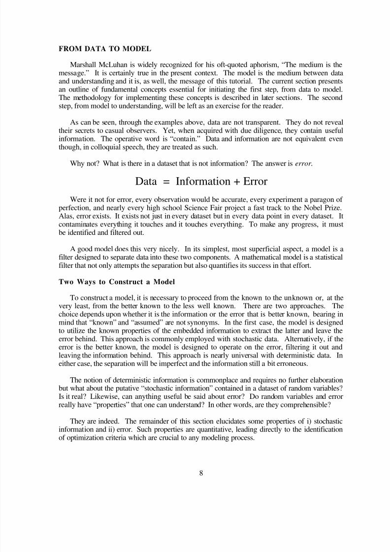
FROM DATA TO MODEL
Marshall McLuhan is widely recognized for his oft-quoted aphorism, “The medium is themessage.” It is certainly true in the present context. The model is the medium between dataand understanding and it is, as well, the message of this tutorial. The current section presentsan outline of fundamental concepts essential for initiating the first step, from data to model.
The methodology for implementing these concepts is described in later sections. The secondstep, from model to understanding, will be left as an exercise for the reader.
As can be seen, through the examples above, data are not transparent. They do not revealtheir secrets to casual observers. Yet, when acquired with due diligence, they contain usefulinformation. The operative word is “contain.” Data and information are not equivalent eventhough, in colloquial speech, they are treated as such.
Why not? What is there in a dataset that is not information? The answer is error .
Data = Information + Error
Were it not for error, every observation would be accurate, every experiment a paragon of perfection, and nearly every high school Science Fair project a fast track to the Nobel Prize.Alas, error exists. It exists not just in every dataset but in every data point in every dataset. Itcontaminates everything it touches and it touches everything. To make any progress, it mustbe identified and filtered out.
A good model does this very nicely. In its simplest, most superficial aspect, a model is afilter designed to separate data into these two components. A mathematical model is a statisticalfilter that not only attempts the separation but also quantifies its success in that effort.
Two Ways to Construct a Model
To construct a model, it is necessary to proceed from the known to the unknown or, at thevery least, from the better known to the less well known. There are two approaches. Thechoice depends upon whether it is the information or the error that is better known, bearing inmind that “known” and “assumed” are not synonyms. In the first case, the model is designedto utilize the known properties of the embedded information to extract the latter and leave theerror behind. This approach is commonly employed with stochastic data. Alternatively, if theerror is the better known, the model is designed to operate on the error, filtering it out andleaving the information behind. This approach is nearly universal with deterministic data. Ineither case, the separation will be imperfect and the information still a bit erroneous.
The notion of deterministic information is commonplace and requires no further elaboration
but what about the putative “stochastic information” contained in a dataset of random variables?Is it real? Likewise, can anything useful be said about error? Do random variables and errorreally have “properties” that one can understand? In other words, are they comprehensible?
They are indeed. The remainder of this section elucidates some properties of i) stochasticinformation and ii) error. Such properties are quantitative, leading directly to the identificationof optimization criteria which are crucial to any modeling process.

8/14/2019 Tutorial Math Modeling
http://slidepdf.com/reader/full/tutorial-math-modeling 13/54
9
Stochastic Information
Stochastic. Information. The juxtaposition seems almost oxymoronic. If something isstochastic (random), does that not imply the absence of information? Can accurate conclusionsreally be induced from random variables?
Well, yes, as a matter of fact. That a variable is stochastic signifies only that its next valueis unpredictable, no matter how much one might know about its history. The data shown inFigure 3 are stochastic in this sense. If you knew the maximum batting average for every yearexcept 1950, that still would not be enough information to tell you the correct value for themissing year. In fact, no amount of ancillary data would be sufficient. This quality is, for allpractical purposes, the quintessence of randomness.
Yet, we have a very practical purpose here. We want to assert something definitive aboutstochastic information. We want to construct models for randomness.
Such models are feasible. Although future values for a random variable are unpredictablein principle, their collective behavior is not. Were it missing from Figure 3, the maximumbatting average for 1950 could not be computed using any algorithm. However, suggestedvalues could be considered and assessed with respect to their probability. For instance, onecould state with confidence that the missing value is probably not less than 0.200 or greaterthan 0.500. One could be quite definite about the improbability of an infinite number of candidate values because any large collection of random variates will exhibit consistency inspite of the randomness of individual variates. It is a matter of experience that the Universe isconsistent even when it is random.
A mathematical model for randomness is expressed as a probability density function(PDF). The easiest way to understand a PDF is to consider the process of computing aweighted average. For example, what is the expectation (average value) resulting from tossing
a pair of ordinary dice if prime totals are discounted? There are six possible outcomes but theyare not equally probable. Therefore, to get the correct answer, one must calculate theweighted average instead of just adding up the six values and dividing the total by six. Thisrequires a set of weights, as shown in Table 3.
Table 3. Weights for Non-prime Totals for Two Dice
Value Weight
4 3/216 5/21
8 5/219 4/2110 3/2112 1/21
The random total, y, has an expected value, denoted <y> or y , given by Equation 3.
8/14/2019 Tutorial Math Modeling
http://slidepdf.com/reader/full/tutorial-math-modeling 14/54
10
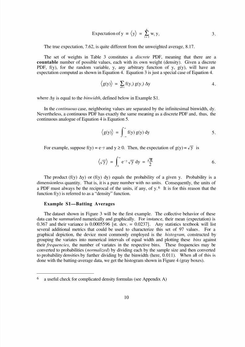
Expectation of y ≡ y = wi y iΣi = 1
6
3.
The true expectation, 7.62, is quite different from the unweighted average, 8.17.
The set of weights in Table 3 constitutes a discrete PDF, meaning that there are a
countable number of possible values, each with its own weight (density). Given a discretePDF, f(y), for the random variable, y, any arbitrary function of y, g(y), will have anexpectation computed as shown in Equation 4. Equation 3 is just a special case of Equation 4.
g(y) = f(y i) g(y i) ∆yΣall i
4.
where ∆y is equal to the binwidth, defined below in Example S1.
In the continuous case, neighboring values are separated by the infinitesimal binwidth, dy.Nevertheless, a continuous PDF has exactly the same meaning as a discrete PDF and, thus, the
continuous analogue of Equation 4 is Equation 5.
g(y) = f(y) g(y) dy
– ∞
∞
5.
For example, suppose f(y) = e–y and y ≥ 0. Then, the expectation of g(y) = y is
y = e– y y dy
0
∞
= π
26.
The product (f(y) ∆y) or (f(y) dy) equals the probability of a given y. Probability is a
dimensionless quantity. That is, it is a pure number with no units. Consequently, the units of a PDF must always be the reciprocal of the units, if any, of y.6 It is for this reason that thefunction f(y) is referred to as a “density” function.
Example S1—Batting Averages
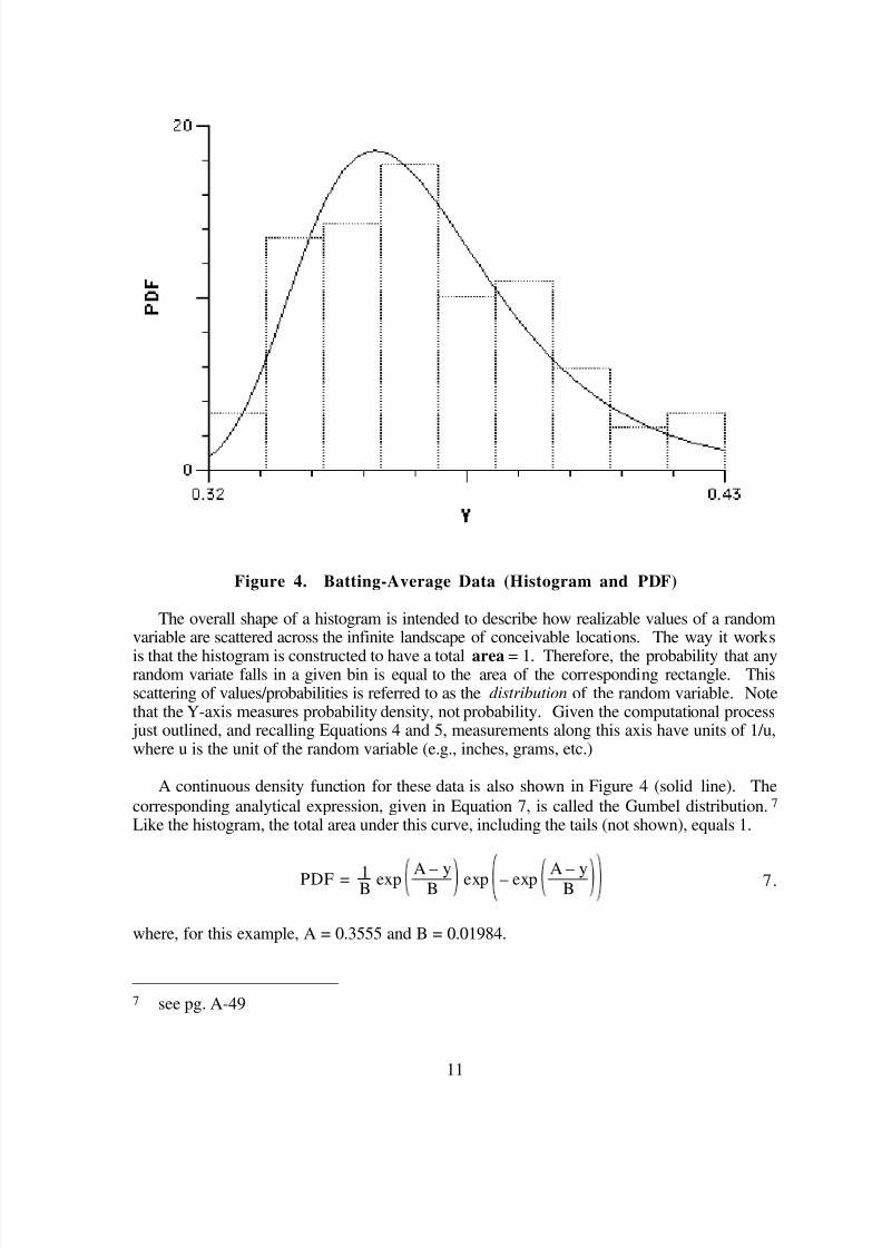
The dataset shown in Figure 3 will be the first example. The collective behavior of thesedata can be summarized numerically and graphically. For instance, their mean (expectation) is0.367 and their variance is 0.0005596 [st. dev. = 0.0237]. Any statistics textbook will listseveral additional metrics that could be used to characterize this set of 97 values. For agraphical depiction, the device most commonly employed is the histogram, constructed bygrouping the variates into numerical intervals of equal width and plotting these bins againsttheir frequencies, the number of variates in the respective bins. These frequencies may beconverted to probabilities (normalized ) by dividing each by the sample size and then convertedto probability densities by further dividing by the binwidth (here, 0.011). When all of this isdone with the batting-average data, we get the histogram shown in Figure 4 (gray boxes).
6 a useful check for complicated density formulas (see Appendix A)
8/14/2019 Tutorial Math Modeling
http://slidepdf.com/reader/full/tutorial-math-modeling 15/54
11
Figure 4. Batting-Average Data (Histogram and PDF)
The overall shape of a histogram is intended to describe how realizable values of a randomvariable are scattered across the infinite landscape of conceivable locations. The way it works
is that the histogram is constructed to have a total area = 1. Therefore, the probability that anyrandom variate falls in a given bin is equal to the area of the corresponding rectangle. Thisscattering of values/probabilities is referred to as the distribution of the random variable. Notethat the Y-axis measures probability density, not probability. Given the computational process just outlined, and recalling Equations 4 and 5, measurements along this axis have units of 1/u,where u is the unit of the random variable (e.g., inches, grams, etc.)
A continuous density function for these data is also shown in Figure 4 (solid line). The
corresponding analytical expression, given in Equation 7, is called the Gumbel distribution.7
Like the histogram, the total area under this curve, including the tails (not shown), equals 1.
PDF = 1B exp A – yB exp – exp A – yB 7.
where, for this example, A = 0.3555 and B = 0.01984.
7 see pg. A-49
8/14/2019 Tutorial Math Modeling
http://slidepdf.com/reader/full/tutorial-math-modeling 16/54
12
We see that Equation 7 does have the proper units. Parameter A has the same units as therandom variable, y. Since any exponent is necessarily dimensionless, parameter B must havethe same units as well. Hence, the entire expression has units of 1/u. Of course, theseparticular data happen to be dimensionless already, but variates described by a PDF usually dohave units of some sort.
The Gumbel distribution is one example of a continuous distribution. [There are manyothers described in Appendix A.] If f(y) is the PDF, the probability of any value of y wouldequal f(y)*dy which, since dy is vanishingly small, is zero. Indeed, intuition demands that theprobability of randomly picking any given value from a continuum must be zero. However,the probability of picking a value in a finite range [a, b] may be greater than zero (Equation 8).
Prob a ≤ y ≤ b = f y dy
a
b
8.
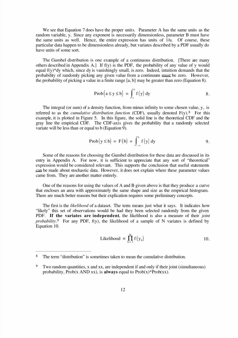
The integral (or sum) of a density function, from minus infinity to some chosen value, y, is
referred to as the cumulative distribution function (CDF), usually denoted F(y).8 For this
example, it is plotted in Figure 5. In this figure, the solid line is the theoretical CDF and thegray line the empirical CDF. The CDF-axis gives the probability that a randomly selectedvariate will be less than or equal to b (Equation 9).
Prob y ≤ b = F b = f y dy
– ∞
b
9.
Some of the reasons for choosing the Gumbel distribution for these data are discussed in itsentry in Appendix A. For now, it is sufficient to appreciate that any sort of “theoretical”expression would be considered relevant. This supports the conclusion that useful statementscan be made about stochastic data. However, it does not explain where these parameter values
came from. They are another matter entirely.
One of the reasons for using the values of A and B given above is that they produce a curvethat encloses an area with approximately the same shape and size as the empirical histogram.There are much better reasons but their explication requires some preliminary concepts.
The first is the likelihood of a dataset. The term means just what it says. It indicates how“likely” this set of observations would be had they been selected randomly from the givenPDF. If the variates are independent, the likelihood is also a measure of their joint
probability.9 For any PDF, f(y), the likelihood of a sample of N variates is defined byEquation 10.
Likelihood ≡ f yk Πk = 1
N
10.
8 The term “distribution” is sometimes taken to mean the cumulative distribution.
9 Two random quantities, x and xx, are independent if and only if their joint (simultaneous)probability, Prob(x AND xx), is always equal to Prob(x)*Prob(xx).

8/14/2019 Tutorial Math Modeling
http://slidepdf.com/reader/full/tutorial-math-modeling 17/54
13
Figure 5. Batting-Average Data (CDF)
The second concept is that of maximum likelihood (ML). This notion is also very intuitive.Given a form for the density function, the ML parameters are those parameters which make the
likelihood as large as possible. In other words, any other set of parameters would make theobserved dataset less likely to have been observed. Since the dataset was observed, the ML
parameters are generally considered to be optimal.10 However, this does not preclude the useof some alternate criterion should circumstances warrant.
The values given above for A and B are the ML parameters. This is an excellent reason forchoosing them to represent the data and it is no coincidence that the theoretical curve in Figure4 matches the histogram so well. Had there been a thousand data points, with proportionatelynarrower histogram bins, the match would have been even better.
Thus, a Gumbel distribution, with these ML parameters, is a model for the data shown inFigure 3. It summarizes and characterizes the stochastic information contained in these data.Not only does it describe the probability density of the data, but one could query the model.One could ask the same questions of the model that could be asked of the data. For example,“What are the average and standard deviation of these data?” or “What is the probability thatnext year’s batting champion will have a batting average within five percent of the historical
10 Their uniqueness is usually taken for granted.

8/14/2019 Tutorial Math Modeling
http://slidepdf.com/reader/full/tutorial-math-modeling 18/54
14
mean?” The answers to such questions may be computed from the model without looking atthe data at all.
For instance, the last question is answered in Equation 11.7
Probability = f y dy
0.95 * mean
1.05 * mean
= F 0.385 – F 0.349 = 0.55 11.
As a check, note that Equation 11 predicts that 53 of the values in Figure 3 are within thegiven range. The data show 52 in this range.
One could even ask questions of the model that one could not ask of the data. For instance,“What is the probability that next year’s batting champion will have a batting average greaterthan the maximum in the dataset (0.424)?” Obviously, there is no such number in the historicaldata and that suggests an answer of zero. However, this is clearly incorrect. Sooner or later,someone is bound to beat 0.424 provided that major-league baseball continues to be played.
It is easy to pose a theoretical question like this to a model and, if the model is good , toobtain a correct answer. This model (Equation 7) gives an answer of three percent, suggestingthat we are already overdue for such a feat.
Whether or not a model is good (valid) is a question yet to be addressed.
Example S2—Rolling Dice
The Gumbel distribution was chosen to model the batting-average data because it is knownto be appropriate, in many cases, for samples of continuous-distribution maxima (so-calledrecord values). However, there is no a priori guarantee that it is valid for these particular data.Occasionally, there is enough known about some type of stochastic information that theory
alone is sufficient to specify one distribution to the exclusion of all others and, perhaps, evenspecify the parameters as well. The second stochastic example illustrates this situation via thefollowing experiment.
Step 1Think of a number, a whole number, from one to six.
Step 2Roll a standard, cubical die repeatedly until your chosen number appears three times.
Step 3Record the number of rolls, Nr, required.
After only a few semesters of advanced mathematics courses, it would be relatively easy to
prove that the random variable, N r, is ~NegativeBinomial(1/6, 3).11 This assertion could be
tested by performing the experiment a very large number of times and comparing the theoreticaldistribution to the empirical data.
11 see pg. A-81; the ~ is read “(is) distributed as”

8/14/2019 Tutorial Math Modeling
http://slidepdf.com/reader/full/tutorial-math-modeling 19/54
15
Carrying out this exercise by hand would be a bit tedious. Fortunately, it is a simple matterto simulate the experiment on a computer. Such simulations are very common. Simulated
results for a 1,000-fold repetition of this experiment are shown in Figure 6.12
Figure 6. Rolls3 Data (Histogram and PDF)
The NegativeBinomial model shown in Figure 6 (solid lines) is another example of adiscrete PDF. Typically, this means that the random variable can take on only integer values.That is the case here since Nr is a count of the number of rolls required.
In computing the model shown, the first parameter was not fixed at its theoretical value,1/6. Instead, it was estimated from the data. The ML estimate = 0.1691, very close to thetheoretical 0.1667. It would have been even closer had the sample size been much larger than1,000. Likewise, the mean predicted by this model = 17.74, very close to the theoreticalmean, 18. The second parameter, 3, was assumed given although it, too, could have beenconsidered unknown and estimated from the data.
The observed data (gray histogram) may be compared to the estimated, ML model using theChi-square statistic, defined in Equation 12.
12 see file Examples:Rolls3.in

8/14/2019 Tutorial Math Modeling
http://slidepdf.com/reader/full/tutorial-math-modeling 20/54
16
Chi–square ≡ χ2 =
o k – e k
2
ek Σall k
12.
where k includes all possible values of the random variable and where o and e are the observedand expected frequencies, respectively.
For this example, Chi-square = 65.235. Again, the question of whether this amount of discrepancy between theory and experiment is “acceptable” is a matter to be discussed below.
Example S3—Normality
We would be remiss in our illustrations of stochastic information were we to omit the mostfamous of all stochastic models, the Normal (Gaussian) distribution. The Normal distributionis a continuous distribution and it arises naturally as a result of the Central Limit Theorem. Inplain English, this theorem states that, provided they exist, averages (means) of any randomvariable or combination of random variables tend to be ~Normal(A, B), where A is the samplemean and B is the unbiased estimate of the population standard deviation. As usual, with
random data, the phrase “tend to” indicates that the validity of this Gaussian model for randommeans increases as the sample size increases.
In Example S2, a thousand experiments were tabulated and individual outcomes recorded.A sample size of 1,000 is certainly large enough to illustrate the Central Limit Theorem. Ourfinal example will, therefore, be a 1,000-fold replication of Example S2, with one alteration.Instead of recording 1,000 values of Nr for each replicate, only their average, N avg, will be
recorded. This new experiment will thus provide 1,000 averages13 which, according to theCentral Limit Theorem, should be normally distributed.
As before, the experiment was carried out in simulation. The observed results and the MLmodel are shown in Figure 7. The estimated values for A and B are 17.991 and 0.2926,
respectively. With a Gaussian model, the ML parameter estimates may be computed directlyfrom the data so one cannot ask how well they match the observed values.
A somewhat better test of the model would be to pick a statistic not formally included in theanalytical form of the distribution. One such statistic is the interquartile range, that is, the rangeincluded by the middle half of the sorted data. In this example, the model predicts a range of
[17.79, 18.19]14 while the data show a range of [17.81, 18.19].
The ideal test would be one that was independent of the exact form of the density function.For continuous distributions, the most common such test is the Kolmogorov-Smirnov (K-S)statistic. The K-S statistic is computed by comparing the empirical CDF to the theoretical
CDF. For example S3, these two are shown in Figure 8. The K-S statistic is simply themagnitude (absolute value) of the maximum discrepancy between the two, measured along theCDF-axis. Here, the K-S statistic = 0.0220.
13 see file Examples:Rolls3avg.in
14 see pg. A-85

8/14/2019 Tutorial Math Modeling
http://slidepdf.com/reader/full/tutorial-math-modeling 21/54
17
Figure 7. Rolls3avg Data (Histogram and PDF)
Figure 8. Rolls3avg Data (CDF)

8/14/2019 Tutorial Math Modeling
http://slidepdf.com/reader/full/tutorial-math-modeling 22/54
18
Once again, the question naturally arises as to whether this result is acceptable and, onceagain, we defer the question until later.
Stochastic Information—Summary
In examples S1 to S3, we have endeavored to show that the term “stochastic information”
is not the contradiction it would appear to be. It should now be clear that random variables arecollectively, if not individually, predictable to a useful extent and that much can be said, withaccuracy, about such variables.
Since much can be said, it follows that it should be possible to use this information to filterout some of the error found in stochastic data. Just because variates are random, it does notmean that they are errorless. The data of Example S1, for instance, appeared to be describedby a Gumbel distribution. However, as with all stochastic datasets, there were discrepanciesbetween model and data. How much of this was due to inherent variation and how much wasdue to error was not discussed. It will be.
Finally, we have described three metrics: the ML criterion, the Chi-square statistic, and theK-S statistic. These three are valid and useful concepts for the description of stochastic dataand it will soon become evident that all may be utilized as optimization criteria as well.
First, however, we discuss deterministic information and the kinds of error commonlyassociated with it.

8/14/2019 Tutorial Math Modeling
http://slidepdf.com/reader/full/tutorial-math-modeling 23/54
19
Deterministic Information and Error
If “stochastic information” seems an oxymoron, “deterministic information” would, forsimilar reasons, appear to be a tautology. Neither is true and, in this discussion, the latter termwill refer to any information gleaned from non-stochastic sources, typically experimentation.Since these sources are prone to error, it is essential to characterize that error in order to attempt
to compensate for it. This section will focus on the kinds of errors found in deterministic data.
The amount of error in a dataset, or even a data point, is generally unknown. The reason,of course, is that error is largely random. We have just seen, however, that randomness doesnot imply total ignorance. To the contrary, modeling of deterministic data usually assumes thatsomething valid is known about the error component of the data, providing a handle withwhich to filter it out. In fact, whenever data of a given type are investigated over an extendedperiod of time, it is not uncommon for associated errors to become as well characterized as theinformation itself.
However, for the purposes of this tutorial, our goals are much less specific. We shall limitour illustrations to a few kinds of error and say something, as well, about error in general. Asin the last section, we seek quantitative metrics that may be employed as optimization criteria.
Components of Error
Empirical datasets, almost without exception, are contaminated with error. Even the datashown in Table 1, which few would dispute, are recorded with limited precision. Therefore,they are subject, at the very least, to quantization error. A dataset without error might beimagined but hardly ever demonstrated.
Not only does a dataset, as a whole, contain an unknown amount of error but every datapoint in it contains some unknown fraction of that total error. Consequently, the amount of
information in a dataset is unknown as well. Each data point makes some contribution to thetotal amount of information but there is no way to tell how much just by looking. Informationand error have the same units and may be physically indistinguishable.
Error comprises some combination of bias and noise. A bias is a systematic deviation fromthe truth due either to a deterministic deviation, consistently applied, or to a random deviationwith a non-zero mean. The former is seen, for instance, when your bathroom scale is notproperly zeroed in. In this case, it will report your apparent weight as too high or too low,depending on the sign of the bias in the zero-point. The latter type of bias is exemplified in thecase of an astronomer who records the image of a distant galaxy by counting the photons thatimpinge on the pixels of a light-sensitive array. Inevitably, each pixel is subject to a counting
error. Such errors are typically random variables ~Poisson(A) and have a mean, A > 0.15
Noise refers either to random, zero-mean errors or to the residual portion of random,biased errors once the bias has been removed. For example, undergraduate chemistrystudents, performing their first quantitative, organic analysis usually get experimental resultsexhibiting lots of errors. These errors are largely random but often have a significant negative
15 see pg. A-101

8/14/2019 Tutorial Math Modeling
http://slidepdf.com/reader/full/tutorial-math-modeling 24/54
20
bias because, in trying to isolate the target substance, some is lost. Quantifying the remainderis a process usually subject to zero-mean, random errors, i.e., noise.
Most often, total error represents the combined effect of several sources of different kindsof error, including biases which can sometimes be identified and removed, as well as noise.To the degree that error is random, only its average effects can be characterized and there is, of
course, no guarantee that a given sample will be average.
As before, we shall eschew theoretical discussions in favor of concrete examples. There isample literature available to anyone wishing to pursue this subject in depth. The examplesbelow all relate to deterministic data.
Example D1—Quantization Error
The daytimes in Table 1 provide an illustration of one kind of error and, at the same time,of the utility of the variance.
One of the most useful properties of the variance statistic is its additivity. Whenever anygiven variance, V, is due to the combined effect of k independent sources of variation, V willequal the sum of the individual variances of these k sources. [Note the recursive nature of thisproperty.]
The variance of the daytimes listed in Table 1 = TSS/N = 836,510/43 = 19,453.72 min 2.As noted above, a portion of this variance derives from the fact that these values, having beenrounded to the nearest minute, have limited precision. This round-off error has nothing to dowith the mechanism responsible for the secular variation in daytime. Hence, the variance dueto rounding (quantization) is independent of all remaining variance, so it can be factored out.
It is easy to demonstrate that quantization error is a random variable ~Uniform[–B, B],
where B is one-half the unit of quantization.16
As such, the variance due to this single sourceof error, Q, is given by Equation 13. For these data, the unit of quantization is one minute.
Therefore, Q = 0.08 min2, only 0.0004 percent of the total variance of the data.
Quantization variance ≡ Q =unit of quantization
2
12 13.
Continually citing squared quantities (with squared units) is inconvenient and the standarddeviation is quoted more often than is the variance. Unfortunately, standard deviations are notadditive. In this example, the “standard deviation of quantization error” is 0.29 min (about 17seconds). Thus, although this quantization error is negligible compared to the overall variation
of the data, it is clearly not negligible when compared to the recorded precision.
If quantization were the only source of error for this dataset, the deterministic informationpresent would constitute 99.9996 percent of the observed variance. It would then be left to thechosen model to “explain” this information. Note that a deterministic model is not expected to
16 see pg. A-113

8/14/2019 Tutorial Math Modeling
http://slidepdf.com/reader/full/tutorial-math-modeling 25/54
21
explain error. That task is delegated to a separate error model, implicitly specified as part of theoptimization procedure.
Finally, the variance statistic is evidently useful not just for computational purposes but, asseen here, as a measure of information. In other words, were the errorless component of thetotal variance equal to zero, there would be nothing to explain. In Example D2, we utilize this
aspect of the variance to develop a quantitative metric for deterministic information explained.
Example D2—Kepler’s First Law
In a deterministic model, the value of the independent variable is supposed to be sufficientto predict the value of the dependent variable to an accuracy matching that of the input. If themodel is important enough, it is often referred to as a law. The implied reverence generallysignifies that something of unusual significance has been discovered about the real world andsummarized in the model so designated. Today, in the physical sciences, laws are particularlyprecise, as are their parameters. In fields related to physics, for instance, it is not uncommonto find model parameters accurate to more than nine significant figures (i.e., one part perbillion). This mathematical approach to understanding we owe, in large part, to the efforts of Johannes Kepler (1571-1630) and Galileo Galilei (1564-1642).
This example was presented by Kepler as an illustration of his First Law, arguably the firstcorrect mathematical model correctly devised. The law states that each planet revolves aboutthe Sun in an ellipse with the Sun at one focus.
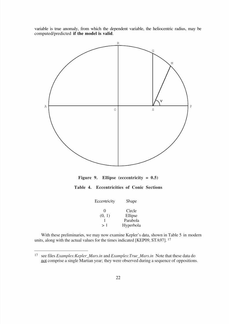
Figure 9 depicts an ellipse, together with some of its more important features. Like anyellipse, its size and shape may be completely specified by two numbers. Usually, one of theseis the length of the semi-major axis, OP, and the other is the eccentricity, which is the ratio of two lengths, OS/OP. The ellipse in the figure has an eccentricity of 0.5 so one focus, S, ishalfway between the center, O, and the circumference at P; the other focus, not shown, is the
mirror image of S through the center.
Kepler spent much of his life investigating the orbit of Mars. This orbit has an eccentricityof only 0.09, so it is much more circular than the ellipse shown in Figure 9 as, indeed, are theorbits of all planets in the Solar System, except Mercury and Pluto. The point P represents thepoint closest to the Sun, S, and is called perihelion; the point farthest from the Sun, A, is calledaphelion. A chord, SG, drawn through a focus and parallel to the semi-minor axis, OR, iscalled the semi-latus rectum. The latter, plus the eccentricity, are the only parameters requiredwhen an ellipse is described in polar coordinates (Equation 14).
radius = A1 + B cos ( ν)
14.
where the origin is at S, from which the radius (e.g., SM) is measured, and where the angle,
ν, measured from perihelion in the direction of motion, is called the true anomaly.
In Equation 14, parameter A is the length of the semi-latus rectum and B is the eccentricity.This equation is actually a general equation describing all of the conic sections—circle, ellipse,parabola, or hyperbola, depending upon the eccentricity (see Table 4). The independent
8/14/2019 Tutorial Math Modeling
http://slidepdf.com/reader/full/tutorial-math-modeling 26/54
22
variable is true anomaly, from which the dependent variable, the heliocentric radius, may becomputed/predicted if the model is valid.
O
A P
M
S
G
R
ν
Figure 9. Ellipse (eccentricity = 0.5)
Table 4. Eccentricities of Conic Sections
Eccentricity Shape
0 Circle(0, 1) Ellipse
1 Parabola
> 1 Hyperbola
With these preliminaries, we may now examine Kepler’s data, shown in Table 5 in modern
units, along with the actual values for the times indicated [KEP09, STA97].17
17 see files Examples:Kepler_Mars.in and Examples:True_Mars.in Note that these data do
not comprise a single Martian year; they were observed during a sequence of oppositions.

8/14/2019 Tutorial Math Modeling
http://slidepdf.com/reader/full/tutorial-math-modeling 27/54
23
Table 5. Orbital Data for Mars
Time Radius (AU) True Anomaly (radians)(JD –
2300000)18
Kepler Predicted Actual Kepler Actual
–789.86 1.58852 1.58853 1.58910 2.13027 2.12831–757.18 1.62104 1.62100 1.62165 2.39837 2.39653–753.19 1.62443 1.62443 1.62509 2.43037 2.42854–726.27 1.64421 1.64423 1.64491 2.64327 2.64152–30.95 1.64907 1.64907 1.64984 2.70815 2.70696
2.84 1.66210 1.66210 1.66288 2.96844 2.9673213.74 1.66400 1.66396 1.66473 3.05176 3.0506549.91 1.66170 1.66171 1.66241 3.32781 3.32675
734.17 1.66232 1.66233 1.66356 3.30693 3.30640772.03 1.64737 1.64738 1.64812 3.59867 3.59818777.95 1.64382 1.64383 1.64456 3.64488 3.64440819.86 1.61027 1.61028 1.61083 3.97910 3.97865
1507.15 1.61000 1.61000 1.61059 3.98145 3.981571542.94 1.57141 1.57141 1.57186 4.28018 4.280351544.97 1.56900 1.56900 1.56944 4.29762 4.297791565.94 1.54326 1.54327 1.54210 4.48063 4.480832303.05 1.47891 1.47889 1.47886 4.94472 4.945652326.98 1.44981 1.44981 1.44969 5.18070 5.181692330.96 1.44526 1.44525 1.44512 5.22084 5.221842348.90 1.42608 1.42608 1.42589 5.40487 5.405913103.05 1.38376 1.38377 1.38332 6.12878 6.130673134.98 1.38463 1.38467 1.38431 0.198457 0.200358
3141.90 1.38682 1.38677 1.38643 0.274599 0.2764973176.80 1.40697 1.40694 1.40676 0.653406 0.6552603891.17 1.43222 1.43225 1.43206 0.940685 0.9432063930.98 1.47890 1.47888 1.47896 1.33840 1.340793937.97 1.48773 1.48776 1.48789 1.40552 1.407883982.80 1.54539 1.54541 1.54583 1.81763 1.81986
Since Kepler intended these data to be illustrative of his law of ellipses, it is reasonable toask whether they are, in fact, described by the model of Equation 14. The graph in Figure 10,
where X is true anomaly and Y is radius, makes it qualitatively apparent that they are.19
This assessment may be quantified by hypothesizing that the information explained by
this model and the residual error constitute independent sources of variation. If this is true,then the total variance of the dataset is the sum of the variances for each of these componentsand it would then be a trivial matter to compare the fraction of the variance/information
18 JD (Julian date) ≡ interval, in days, from Greenwich noon, 1 January 4713 B.C.
19 The ellipse, in this (optimized) model, has A = 1.51043 AU and B = 0.0926388.

8/14/2019 Tutorial Math Modeling
http://slidepdf.com/reader/full/tutorial-math-modeling 28/54
24
explained by this model to the total variance in the dataset. A good model is one that leavesrelatively little unexplained.
Figure 10. Kepler’s Data and Model
Since the number of points is constant throughout this example, we may substitute sums of squares for the respective variances. The information not explained by the model, plus thevariance due to any errors, is then equal to the error-sum-of-squares, ESS, often called theresidual-sum-of-squares, defined in Equation 15.
Error-sum-of-squares ≡ ESS = y i – y i
2
Σi = 1
N
15.
where y is the value predicted by the model.
Therefore, the fraction of the total variance in the dataset that is explained by a given model
is equal to the statistic R-squared , defined in Equation 16.
R-squared = 1 – ESSTSS
16.
Kepler’s data, plus the predictions of the optimum model (Table 5, column 3), produce thefollowing results (computed to six significant figures):

8/14/2019 Tutorial Math Modeling
http://slidepdf.com/reader/full/tutorial-math-modeling 29/54
25
TSS = 0.273586 AU2
ESS = 1.257e–08 AU2
R-squared = 1.00000
In other words, by this statistic/criterion, the model described in Equation 14 and Figure 10explains all of the deterministic information contained in Kepler’s dataset to a precision of one
part in 100,000.
This result is not quite perfection. Since ESS > 0, there remains something, true deviations
or error, yet to be explained.20 Also, the 28 radii listed by Kepler are not really as accurate ashis values indicate. Nevertheless, this degree of success is impressive. There are thousands of sociologists, psychologists, and economists who would be more than delighted with results of such precision.
We shall see later how Kepler’s model was optimized to find parameters yielding this valuefor R-squared.
Example D3—World Track Records
As a measure of information and/or error, the variance statistic reigns supreme in most of contemporary analysis of deterministic data. However, intuition suggests that the “best”deterministic model is the one that minimizes the average deviation, defined in Equation 17.When graphed, this model gives the curve that is as close as possible to all of the data pointssimultaneously, using a statistic with the same units as the dependent variable.
Average Deviation = 1N
y i – y iΣi = 1
N
17.
where y is the value predicted by the model.
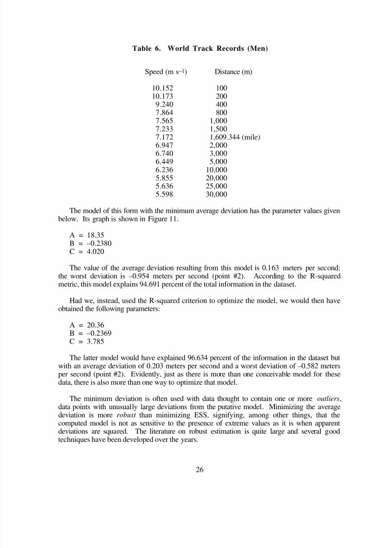
To illustrate this metric, consider the data in Table 6.21 This table lists 14 distances forwhich world track records (for men) are recognized. The corresponding average speed attainedduring each record run is listed as well [YOU97]. The task is to model this speed as a functionof distance.
Not surprisingly, the average speed decreases sharply, at first, but then seems to level off somewhat. Many analytical forms would be suitable but we shall examine the power law givenin Equation 18 (where y is speed and x is distance).
y = A xB + C 18.
20 That this “something” is relatively small does not imply that it is spurious or insignificant.
21 see file Examples:Track.in
8/14/2019 Tutorial Math Modeling
http://slidepdf.com/reader/full/tutorial-math-modeling 30/54
26
Table 6. World Track Records (Men)
Speed (m s–1) Distance (m)
10.152 100
10.173 2009.240 4007.864 8007.565 1,0007.233 1,5007.172 1,609.344 (mile)6.947 2,0006.740 3,0006.449 5,0006.236 10,0005.855 20,0005.636 25,000
5.598 30,000
The model of this form with the minimum average deviation has the parameter values givenbelow. Its graph is shown in Figure 11.
A = 18.35B = –0.2380C = 4.020
The value of the average deviation resulting from this model is 0.163 meters per second;the worst deviation is –0.954 meters per second (point #2). According to the R-squared
metric, this model explains 94.691 percent of the total information in the dataset.
Had we, instead, used the R-squared criterion to optimize the model, we would then haveobtained the following parameters:
A = 20.36B = –0.2369C = 3.785
The latter model would have explained 96.634 percent of the information in the dataset butwith an average deviation of 0.203 meters per second and a worst deviation of –0.582 metersper second (point #2). Evidently, just as there is more than one conceivable model for these
data, there is also more than one way to optimize that model.
The minimum deviation is often used with data thought to contain one or more outliers,data points with unusually large deviations from the putative model. Minimizing the averagedeviation is more robust than minimizing ESS, signifying, among other things, that thecomputed model is not as sensitive to the presence of extreme values as it is when apparentdeviations are squared. The literature on robust estimation is quite large and several goodtechniques have been developed over the years.

8/14/2019 Tutorial Math Modeling
http://slidepdf.com/reader/full/tutorial-math-modeling 31/54
27
Figure 11. World Track Records
Deterministic Information—Summary
In this section, we have described two metrics for deterministic modeling, giving differentanswers. Is the choice a matter of indifference or is one better than the other?
To anyone trying to understand the real world, there can be only one “best” answer becausethere is only one Universe. Nature does not use one set of rules on weekdays and another onweekends. To be credible, a model must eschew arbitrariness to the greatest extent possible.Moreover, it must be completely consistent with whatever is already known about the data itdescribes, including even aspects of the data that are not the subject of the model.
As noted earlier, any deterministic model should be optimized utilizing whatever is knownabout the errors in the data. In Examples D2 and D3, this concern was not addressed. So far,we have considered only the fraction of information explained and average deviation (error),
without considering specific properties of the residual variance. Finally, in discussing thesetwo models, we did not relate much of what we said about stochastic modeling, especially thepowerful concept of maximum likelihood, to the fact that errors in data are largely random.
In the next section we shall put everything together. Our efforts will be rewarded with a setof valid, intuitive, and well-defined criteria for computing optimum model parameters.

8/14/2019 Tutorial Math Modeling
http://slidepdf.com/reader/full/tutorial-math-modeling 32/54
28
FINDING OPTIMUM PARAMETERS
Data, as we have seen, come in two varieties: stochastic and deterministic. Each of thesemay be modeled and that model characterized by one of a number of metrics (statistics) relatingsomething about the quality of the model. Quality implies descriptive or explanatory power,proof of which is manifested in predictive capability. All of this presupposes, of course, that
models exhibiting these desiderata can actually be found.
This section clarifies some relationships among the five metrics described earlier. In doingso, a general technique for finding optimum parameters will be cited. It will be apparent thatthis technique may be readily implemented as a computational algorithm.
Five Criteria
The five metrics/statistics that we shall utilize as modeling criteria are listed in Table 7. Thetwo primary criteria are shown in bold and their preeminence will be discussed.
Table 7. Modeling Criteria
Criterion Applicability
Maximum likelihood All random variatesMinimum K-S statistic Continuous random variates
Minimum chi-square statistic Discrete random variates
Minimum ESS (least squares) Deterministic dataMinimum average deviation Deterministic data
Some of the reasons why these five are desirable criteria were described in the last section.It was taken for granted there that, given an appropriate analytical form for the model, findingparameters that would optimize the chosen metric was practicable. Indeed, most of the valuesfor model parameters given in the text are illustrative.
The methodology described here takes a modeling criterion as a kind of meta-parameter.Partial justification for this approach derives from the fact that these five criteria are moreinterrelated than they might appear. In particular, as first demonstrated by Carl FriedrichGauss (1777-1855) and Adrien Marie Legendre (1752-1833), there are deep, fundamentalconnections linking the criteria for stochastic and deterministic modeling. These relationshipsare due to the randomness of error.
Maximum Likelihood Redux
In the course of any description of modeling and statistics, it is easy to get lost in the almostinevitable deluge of symbology and equations and, in the confusion, lose sight of the originalobjective. One is dealing, presumably, with real data from the real world. Thus, a model isnot just some computational gimmick for reproducing a matrix of numbers. A good modelsays something genuine about the Universe. Its analytical form is discovered, not invented; itsparameters are properties of Nature, not the whim of an analyst.

8/14/2019 Tutorial Math Modeling
http://slidepdf.com/reader/full/tutorial-math-modeling 33/54
29
The ML criterion acknowledges this role, as well as the supremacy of data, in the mostdirect fashion. Given the form for a stochastic model, ML parameters maximize the probabilitythat the observed data came from a parent population described by the model. Deterministicmodeling, on the other hand, attempts to maximize the explanatory power of the model or,occasionally, to minimize the average deviation. It turns out that there is a profound connectionbetween least squares (also, minimum deviation) and maximum likelihood.
We shall start with least squares. This is undoubtedly the most widely used of all modelingcriteria. It is usually presented simply as a technique for generating a curve that is closest to allof the data points. Of course, it isn’t. The minimum-deviation criterion is the one that yieldsthat particular curve. As we have seen, the least-squares technique actually minimizes the errorvariance and, hence, maximizes the fraction of information that is explained by the model. If it did nothing else, one could hardly complain. However, it does much more.
In real life, errors are almost never simple manifestations of a single mechanism. Nearlyalways, the total error in an observation is the net effect of several different errors. As a result,the Central Limit Theorem takes over and stipulates that such errors have a strong tendency tobe ~Normal(A, B). This theorem was illustrated in Example S3.
In devising a deterministic model, suppose that this theorem and the proliferation of errormodes are taken at face value. Then one might ask, “What set of parameter values maximizesthe likelihood of the residuals if they are normally distributed? Also, is this vector unique?”
Thus, assume that the residuals for the data points, εk ≡ yk – yk , are ~Normal(Ak , Bk ). In
addition, assume that these residuals are all unbiased so that Ak is always zero. Then, the
likelihood is given by Equation 19 (cf. Eq. 10 and pg. A-85).
Likelihood ≡ f εk Π
k = 1
N
= 1
Bk 2π
exp – 1
2
εk
Bk
2
Πk = 1
N
19.
Equation 19 can be simplified. The log() function is monotonic, so any set of parametersthat maximizes log(likelihood) will necessarily maximize the likelihood. Taking (natural) logsof both sides of Equation 19 produces Equation 20.
Log-likelihood = – log B k 2 πΣk = 1
N
– 12
εk
Bk
2
Σk = 1
N
20.
Given a set of measurement errors, the first term in Equation 20 is a constant and has nobearing on the maximization. The likelihood will be a maximum if and only if the expression
in Implication 21 is a minimum.
Maximum likelihood ⇒ min
εk
Bk
2
Σk = 1
N
21.
If the errors for all of the points come from the same normal distribution, then all Bk are equal
and, after canceling the units, this constant can be factored out giving Implication 22.

8/14/2019 Tutorial Math Modeling
http://slidepdf.com/reader/full/tutorial-math-modeling 34/54
30
Maximum likelihood ⇒ 1
Bmin εk
2Σk = 1
N
⇒ min yk – yk
2
Σk = 1
N
22.
However, the term on the far right is just ESS! In other words,
if all errors are ~Normal(0, B), then the parametersthat minimize ESS are the very same parameters thatmaximize the likelihood of the residuals.
It turns out that this vector of parameters is almost always unique. The least-squaresparameters have many other useful properties as well but these lie beyond our present scope.
While this is a wonderful result, it falls short of perfection for at least two reasons. First,the fact that the parameters are the ML parameters says nothing about the analytical form of themodel. If the model itself is inappropriate, its parameter values are academic. Second, there isno guarantee that the errors are independent or normally distributed. These hypotheses must beproven for the least-squares method to yield the ML parameters.
However, the strong assumption that all Bk are equal is unnecessary provided that their
true values are known. Minimizing Implication 21, instead of Implication 22, is referred
to as the weighted least-squares technique.22
Finally, what about the minimum-deviation criterion? Can that be related to the maximum-likelihood function as well?
Yes, it can. The second most common distribution for experimental errors is the Laplacedistribution (see pg. A-63). Substituting the Laplace density for the Normal density, thederivation above produces Implication 23 instead of Implication 21.
Maximum likelihood ⇒ min
yk – y k
Bk Σ
k = 1
N
23.
Implication 23 is equivalent to minimizing the (weighted) average deviation, analogous toweighted least squares. Of course, the same caveats apply here as in the case of normal errors.
Alternate Criteria
The two criteria that do not relate directly to maximum likelihood are the minimum K-Scriterion and the minimum chi-square criterion. Nevertheless, the first of these is justified
because it is the most common goodness-of-fit test for continuous random variates, as well asone of the most powerful. The chi-square criterion is the discrete counterpart of the K-Scriterion and any discussion of discrete variates would be very incomplete without it.
22 Some texts discuss only the latter since setting all Bk equal to one is always a possibility.

8/14/2019 Tutorial Math Modeling
http://slidepdf.com/reader/full/tutorial-math-modeling 35/54
31
From this point on, we shall take it as given that the criteria listed in Table 7 are not onlyvalid and appropriate but, in many respects, optimal. The next task is, therefore, to computethe parameters that realize the selected criterion.
Searching for Optima
As noted earlier, a single computational technique will suffice regardless of the selectedcriterion. All optimizations of this sort are essentially a search in a multidimensional parameterspace for values which optimize the objective function specified by this criterion. There aremany generic algorithms from which to choose. One of the most robust is the simplex method
of Nelder and Mead.23
The simplex algorithm traverses the parameter space and locates the local optimum nearestthe starting point. Depending upon the complexity of the parameter space, which increasesrapidly with dimensionality, this local optimum may or may not be the global optimumsought. It is, as always, up to the analyst to confirm that the computer output is, in fact, thedesired solution.
The simplex is a common algorithm and source code is readily available [CAC84, PRE92].
Summary
Three of the five modeling criteria described in the first section have been shown to beclosely linked to the concept of maximum likelihood. Consequently, they are eminentlysuitable as modeling criteria. They are intuitive, valid, and appropriate. Moreover, they almostalways provide unique parameter vectors for any model with which they are employed.
Two other criteria were also listed. Both of these are best known as goodness-of-fit criteriafor random variates with respect to some putative population density. However, they may also
be employed to determine the parameters for this density, not just to test the final result.
The simplex algorithm will prove suitable, in all cases, to compute parameters satisfyingthe chosen criterion in any modeling task that we shall address. The truth of this assertion hasnot yet been demonstrated but it will become evident in the sections to follow. Some of thefigures shown above provide examples.
To this point, we have seen, or at least stated, how models may be specified, optimized,and computed. The stage is now set to evaluate the results of any such endeavor. We shalldiscuss the quality of models in general and of their parameters in particular. Is the model anygood? Are the parameters credible? Does the combination of model and parameters makesense in the light of what we know about this experiment and about the Universe in general?
In other words, are we doing real science/engineering/analysis or are we just playing with data?
23 not to be confused with the linear programming technique of the same name
8/14/2019 Tutorial Math Modeling
http://slidepdf.com/reader/full/tutorial-math-modeling 36/54
32
IS THE MODEL ANY GOOD?
The “goodness” of a model depends not on how well it might serve our purposes but onthe degree to which it tells the truth. Beauty, in this case, is not entirely in the eye of thebeholder. If a model is based upon observed data, especially physical data about the realworld, then the model must be equally real. Several criteria have been established, in earlier
sections, that measure the validity (i.e., the reality) of a model. In this section, we shall focusmainly on the statistical dimension of this reality; the physical dimension is beyond our scope.
Deterministic data and stochastic data will be treated separately because the former case isvery easy but the latter is not. However, as we have seen, it is the modeling of error as arandom variable that lends credence to the aforementioned deterministic criteria. Thus, thevalidity of stochastic models is fundamental to the validity of modeling in general.
In this section, we encounter a new technique—the bootstrap. The bootstrap may be parametric or nonparametric. In the discussions to follow, both forms will be employed. Theutility of these techniques should be self-evident.
The Bootstrap
Since there is ample literature on bootstrap methodology [EFR93], the descriptions herewill be somewhat abbreviated. While the name is fairly new, some of what is now termed“bootstrap” methodology is not. In particular, the parametric bootstrap includes much that wasformerly considered simply a kind of Monte Carlo simulation. However, the nonparametricbootstrap, outlined in the next section, is quite recent.
The bootstrap technique was designed, primarily, to establish confidence intervals for agiven statistic. A confidence interval is a contiguous range of values within which the “true”value of the statistic will be found with some predetermined probability. Thus, the two-sided,
95-percent confidence interval for a given K-S statistic is that range of values within which thetrue K-S statistic will be found in 95 percent of all samples drawn from the given population,being found 2.5 percent of the time in each tail outside the interval. Other things being equal,the width of this interval decreases with increasing sample size.
Sometimes, a confidence interval may be computed from theory alone. For instance,means of large, random samples tend to be unbiased and normally distributed. Therefore, the
95-percent confidence interval for any such mean is just µ ± 1.96 SE, where µ is the observed
mean and SE is the standard error of the mean, given by Equation 24.
SE = σ
N24.
where σ is the population standard deviation for the data and N is the sample size.
As an example, consider again the data exhibited in Figure 7. Theory says that these 1,000means should, themselves, have an (unbiased) mean of 18 and a standard deviation (SE) of
0.30. Hence, 95 percent of them should lie in the interval 18 ± 1.96*0.30 = [17.41, 18.59],
with the remaining five percent divided equally between the two tails. In fact, if you sort thefile Examples:Rolls3avg.in, you will find that these 1,000 means exhibit a 95-percent central

8/14/2019 Tutorial Math Modeling
http://slidepdf.com/reader/full/tutorial-math-modeling 37/54
33
confidence interval of [17.40, 18.55]. The latter interval is, of course, just a sample of sizeone of all similar confidence intervals for similar data. As such, it is expected to deviate a littlebit from theory. If you sense a little recursion going on here, you are quite right.
What we have just done, without saying so, was a form of parametric bootstrap. The fileof 1,000 means was obtained by simulating the original experiment 1,000 times. Each trial
was terminated when an event with a probability of 1/6 was realized 3 times. The simulationused these two parameters to synthesize 1,000 bootstrap samples, each sample containing1,000 trials, with only the sample mean recorded. The explicit use of input parameters makesthis a parametric bootstrap.
Figures 7 and 8, and the accompanying discussion, illustrate not only the Central LimitTheorem but also the validity of the bootstrap technique. This technique has received a greatdeal of scrutiny over the past decade, with very positive results. We shall put it to good use.Almost all of our remaining discussion will derive from the now well-established fact that
bootstrap samples are valid samples.
Whether they are created from theory (parametric bootstrap) or experiment (nonparametricbootstrap), bootstrap samples constitute additional data. These data may be characterized byone or more statistics and the ensuing distribution of these statistics utilized to estimate anydesired confidence intervals. By comparing optimum values, for any model, to the confidenceintervals for these values, the probability of the former may be estimated. In this section, thisprobability will be related to goodness-of-fit; in the following section, it will be employed toestimate parameter uncertainty.
Stochastic Models
Table 7 listed three criteria for optimizing a stochastic model. Unlike their deterministic
counterparts, none of these criteria are self-explanatory. In general, it is not easy to tell, fromthe value of the given statistic, whether or not that value is probable under the hypothesis thatthe optimum model is valid.
For example, the K-S statistic for the best-fit Gumbel distribution to the Batting-Averagedata is 0.057892. This number represents the maximum (unsigned) discrepancy between thetheoretical and empirical CDFs. So much is very clear. What is not at all clear, however, iswhether or not a random sample (N = 97) from a genuine population described bythe same distribution would be likely to exhibit a K-S statistic having the same value. Itcould be that the value 0.057892 is too large to be credible.
How could you tell? The traditional approach would be to look up a table of K-S critical
points in a reference and compare the observed value to some table entry. The problem withthis approach is that nearly all such tables list asymptotic results, i.e., with N = Infinity. Eventhose that have entries for specific sample sizes are not always appropriate in every case. Theremight be hidden dependencies on model form or parameters that could invalidate the recordedcritical points. Ideally, what one would really like is a made-to-order table, conditioned on thesample size, the model form, and the model parameters. Before the advent of fast digitalcomputers, such a table was a rare luxury. Today, it is fairly easy.

8/14/2019 Tutorial Math Modeling
http://slidepdf.com/reader/full/tutorial-math-modeling 38/54
34
To construct such a customized table, we start with the putative parent population. In thiscase, we start with the Gumbel distribution given in Equation 25.
PDF = 1
0.01984exp
0.3555 – y
0.01984exp – exp
0.3555 – y
0.0198425.
From this distribution, which purports to be a good description of our data, draw a randomsample (N = 97) a very large number of times (at least 1,000 times). With each of thesesamples, carry out the same operations that were performed on the original data.Here, we assume that each sample is ~Gumbel(A, B) and we optimize the model, for eachsample, using our original criterion. When all of this is done, we have a vector of 1,000bootstrapped K-S statistics, all of which a) genuinely reflect our candidate population, byconstruction, and b) were obtained exactly as was the original K-S statistic.
There are now several ways to proceed but, here, we shall adopt the simplest approach.First, sort the 1,000 bootstrapped statistics in ascending order. The result will look much like
the histogram in Figure 12 (where Y = K-S statistic).
Figure 12. Distribution of K-S Statistic from Equation 25

8/14/2019 Tutorial Math Modeling
http://slidepdf.com/reader/full/tutorial-math-modeling 39/54
35
The bootstrapped K-S statistic is, itself, a random variable and we could try to model it.
Since each of these continuous variates represents the maximum of 2 x 97 comparisons,24 they
might even be ~Gumbel(A, B)!25 However, we shall instead use just the raw values. It turnsout that our observed value of K-S is found in the 41 st percentile of this specific K-Sdistribution. In other words, if you draw a sample (N = 97) from the distribution given byEquation 25, model it as ~Gumbel(A, B), and recompute the optimum A and B using the MLcriterion then, 59 percent of the time, the K-S statistic you will get will be larger (worse) thanthe one we obtained with the Batting-Average data.
It is customary to require the 95th percentile before rejecting an hypothesis which meansthat we cannot reject the null hypothesis that our data are modeled by Eq. 25. While notrejecting an hypothesis is not quite the same thing as accepting it, in practice, this is the usualinterpretation. Therefore, we conclude that
according to the K-S test, Eq. 25 is an ACCEPTABLE description of our data.
We could go through the same procedure with the 1,000 Log-likelihood statistics that
resulted from this bootstrap process, assessing the observed value in the same fashion. Then,we would have two measures of acceptability. The prudent course would be to require both of them to be acceptable before declaring that the model is good. In this example, the observed
value falls in the 47th percentile of its (bootstrapped) distribution so it, too, is acceptable.
With discrete variates, the usual goodness-of-fit statistic is Chi-square. The sameprocedure would apply there as well. In fact, the bootstrap technique is a very general methodfor assessing goodness-of-fit, no matter what statistic/criterion is used.
There is also a simple rule-of-thumb when using the Chi-square statistic as described. Its
expected value is equal to the number of degrees of freedom.26 Therefore, if the Chi-squarevalue found is less than the range of y-values, it will always be acceptable.
Deterministic Models
Since the bootstrap technique is generally valid, it could be used for assessing goodness-of-fit with deterministic models as well. However, R-squared, the usual statistic in such cases,is self-explanatory. It is equal to the fraction of the variance explained by the model. There isno need to ask about the probability of such a value with a given dataset/model combination.
The minimum-deviation statistic is not quite as transparent. Still, this statistic has the sameunits as the data and it is usually easy to tell if a given minimum deviation is small enough forthe intended purposes.
24 Each end of each “step” in the empirical CDF must be examined.
25 Indeed they are, Gumbel(0.05604, 0.01192) [Fig. 12, solid line]. In fact, this model is aneven better fit than it was with the Batting-Average data. See also, Examples:KStest.in.
26 see pg. A-42

8/14/2019 Tutorial Math Modeling
http://slidepdf.com/reader/full/tutorial-math-modeling 40/54
36
All of the above is true whether the deterministic modeling (regression) is weighted orunweighted. With weighted regressions, the weighted residuals take the place of the usualresiduals since the former are now normalized with respect to their own standard errors.However, the goodness-of-fit metrics, and their meaning, remain the same.
Summary
This section has outlined a general technique for establishing the validity of a mathematicalmodel. If a model is deemed acceptable, it signifies that the equation (or density function) maysubstitute for the original data. Moreover, the model may now be queried, perhaps in waysthat would be impossible with the actual dataset. Deterministic models may likewise be used tointerpolate or extrapolate from the observed values. In short, if a model is acceptable, it isequivalent to any and all past (or future) observations.
With stochastic models, acceptability is assessed by comparing one or more goodness-of-fit statistics (random variables) to their respective distributions, asking whether the valueobserved is too improbable to credit. With deterministic models, the goodness-of-fit statisticsare sufficiently perspicuous that we need not go to so much trouble.
Once again, it must be emphasized that none of this is meant as some kind of mathematicalgimmick. The number of potential models is infinite and, with enough fortitude, any datasetcould be adequately fit to one or more of them. The real goal is to find the model that Natureuses by examining a sample of observations. The techniques described herein are immenselypowerful but they are blind. The necessary vision must be supplied by the analyst.
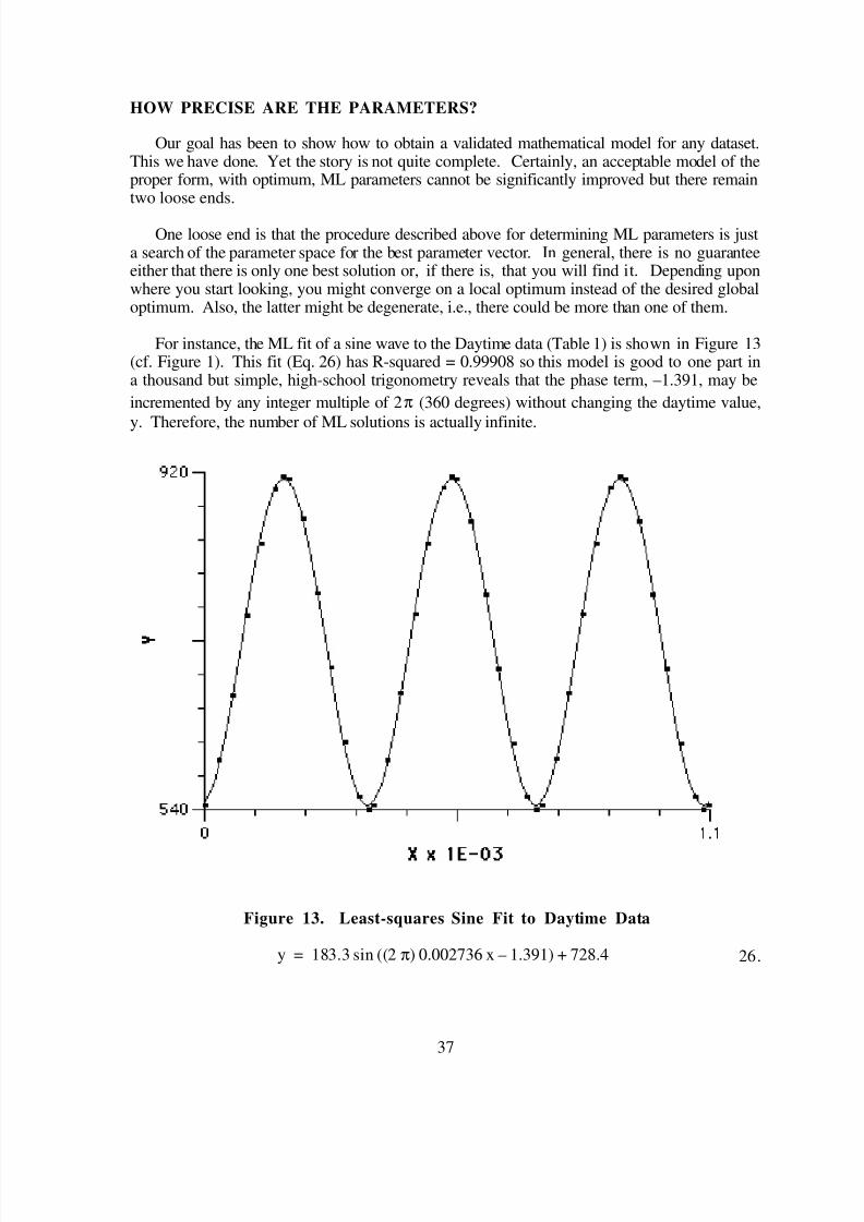
8/14/2019 Tutorial Math Modeling
http://slidepdf.com/reader/full/tutorial-math-modeling 41/54
37
HOW PRECISE ARE THE PARAMETERS?
Our goal has been to show how to obtain a validated mathematical model for any dataset.This we have done. Yet the story is not quite complete. Certainly, an acceptable model of theproper form, with optimum, ML parameters cannot be significantly improved but there remaintwo loose ends.
One loose end is that the procedure described above for determining ML parameters is justa search of the parameter space for the best parameter vector. In general, there is no guaranteeeither that there is only one best solution or, if there is, that you will find it. Depending uponwhere you start looking, you might converge on a local optimum instead of the desired globaloptimum. Also, the latter might be degenerate, i.e., there could be more than one of them.
For instance, the ML fit of a sine wave to the Daytime data (Table 1) is shown in Figure 13(cf. Figure 1). This fit (Eq. 26) has R-squared = 0.99908 so this model is good to one part ina thousand but simple, high-school trigonometry reveals that the phase term, –1.391, may be
incremented by any integer multiple of 2π (360 degrees) without changing the daytime value,
y. Therefore, the number of ML solutions is actually infinite.
Figure 13. Least-squares Sine Fit to Daytime Data
y = 183.3 sin ((2 π) 0.002736 x – 1.391) + 728.4 26.

8/14/2019 Tutorial Math Modeling
http://slidepdf.com/reader/full/tutorial-math-modeling 42/54
38
The other loose end stems from the definition of maximum likelihood. ML parameters are,by definition, more probable than any others—but how probable is that? Suppose you proposeto flip a coin 100 times and bet on the outcome. The wise bet would be 50 Heads and 50 Tailsbecause that is the ML result; every other result is less likely. Suppose, however, that somebystanders are watching all of this and decide to bet, amongst themselves, whether or not youwill win your bet. The wise choice in this case would be to bet that you would lose. Even
though, with a fair coin, a 50:50 outcome is the most probable, its probability is still less thaneight percent. There are just too many other possibilities for any one of them to be at all likely.So your chances of losing are, at best, more than 92 percent.
The probability that the ML parameters in a model are equal to the true parameters is evenworse. Unless theory insists that a given parameter must be a rational number, then you can beabsolutely certain that the optimum value you found for it will always be incorrect. Thereason, noted earlier, is that selecting a specific number from the real domain has a probability
of zero. You can never do it exactly.27
But you can get as close as you like. All it takes is a lot of effort and a very large sample.
Sampling is the key. The model for the radius of the orbit of Mars (Table 5, col. 3) as afunction of true anomaly has two ML parameters: A = 1.51043 AU and B = 0.0926388. TheKeplerian model is an approximation, albeit a very good one, to the true solution.Nevertheless, even if we grant that the elliptical approximation is good enough, these twoparameters are not perfect. Were new data found for exactly the same time frame, theseparameters would be different even though the orbit of Mars was constant . Everydataset is a sample, not the entire population. Therefore, there is always some sampling error.
Nothing can be done to compensate for degenerate global optima except to examine the MLparameters for reasonableness. They must make sense! They must have the correct units andbe consistent with what is known about the real world. This is essential even if the solution is
not degenerate. Likewise, parameter uncertainties due to sampling error, or to deficiencies inthe model, cannot be removed once the ML result has been obtained. However, they can beestimated.
The purpose of this section is to describe a procedure for estimating parameter uncertainty.In addition, parameter correlation is also discussed. The latter is a subtle kind of uncertaintywhich recognizes that parameters are not necessarily independent. We shall take it as given thatthe model is acceptable since a model that is not acceptable is of little interest and its parameterseven less so.
To quantify uncertainty, we shall utilize confidence intervals. Every optimum parametercan be assigned a confidence interval within which the true value of the parameter will be found
with some specified probability. The wider this confidence interval, the more uncertain theparameter value.
27 assuming that you cannot go out and examine every member of the parent population

8/14/2019 Tutorial Math Modeling
http://slidepdf.com/reader/full/tutorial-math-modeling 43/54
39
As we have already seen, confidence intervals may be estimated via the bootstrap. For thisapplication, however, the parametric bootstrap is not suitable. We are not asking now about atheoretical population from which we can select random variates. Rather, we are asking aboutone particular dataset, the one that gave rise to the model. Hence, we need a nonparametricbootstrap that somehow uses this dataset to generate further bootstrap samples. The requisitemethodology is outlined below. As we have done throughout this tutorial, we concentrate on
examples instead of theory, first with stochastic models, then with deterministic models.
The Nonparametric Bootstrap
A nonparametric bootstrap sample is created by resampling the original dataset,with replacement. Imagine that the original data are in a paper bag. Close your eyes andselect one point/variate from the bag, record its value, then put it back . Repeat this selectionuntil you have a sample of the same size as the original. Such a sample is nonparametric; itcomes from the actual data, not from a parametric model of that data. Reusing the data in this
way might seem like cheating28 but it is quite valid, as long as proper corrections are applied.
In the previous section, when we discussed the parametric bootstrap, a simple approachwas used to analyze the bootstrap distributions. For instance, consider the 1,000 K-S statisticsin Figure 12. These 1,000 values constitute an empirical CDF for any K-S statistic computedfor a sample (N = 97) that is ~Gumbel(0.3555, 0.01984). To determine a central, 95-percentconfidence interval for K-S, using the percentile method, we throw away the 25 largest and25 smallest of these 1,000 K-S values. The remaining 0.95*1,000 = 950 values comprise thedesired confidence interval, conditioned on this model and the given sample size . Its range is[0.0401747, 0.0974331]. Its interpretation is that 95 percent of the K-S statistics you wouldobtain with a genuine sample (N = 97) from this Gumbel distribution would fall in this range.Furthermore, 2.5 percent would fall in the range [0, 0.0401747] and the last 2.5 percent in therange [0.0974331, 1].
Were the model or sample size different, the 95-percent confidence interval would bedifferent. The confidence interval would also grow or shrink with the need for increased ordecreased confidence, respectively. Thus, the 90-percent confidence interval in this example is[0.0430050, 0.0901146] and the 99-percent confidence interval is [0.0364837, 0.107393].
With the nonparametric bootstrap, it is better not to use such a simple approach to find aconfidence interval. When the original data are resampled, the resulting bootstrap distributionis biased and skewed. The corrections referred to above compensate for these defects. Insteadof using the 25th and 975th elements of the sorted CDF to demarcate the tails of the bootstrap
distribution, the BCa technique specifies alternate indices.29 Once these have been identified,however, the interpretation of the confidence interval remains the same.
We shall now illustrate the use of these nonparametric confidence intervals to determine theprecision (confidence) that we may ascribe to the ML parameters of any model.
28 or, at least, “pulling oneself up by one’s bootstraps”
29 Computing the latter is well understood but rather complicated [see Technical Details].

8/14/2019 Tutorial Math Modeling
http://slidepdf.com/reader/full/tutorial-math-modeling 44/54
40
Stochastic Models
Repeat the following procedure 50 times:
Step 1Let X and Y be random Cartesian coordinates ~Normal(0, 3).
Step 2Select X and Y, then draw the radius, R, from the origin to the point (X, Y).
Step 3Record the length of R.
At the end of this experiment, we have a sample of 50 values for R.30 Although we shall
not prove it, theory says that R is ~Rayleigh(3) which is the same as ~Chi(3, 2). 31 However,let us pretend that we know that the distribution should be Rayleigh but have forgotten how tocompute the theoretical scale parameter, A. Instead, we shall just determine the ML parameterfor a Rayleigh(A) model (Equation 27), based upon this small sample.
PDF = yA2 exp – 1
2yA
2
27.
The result (see Figure 14, with Y representing R) is quite acceptable, but with A = 2.847instead of 3. What happened? Did we make a mistake? Is the theory wrong? Was ourpseudo-random number generator faulty?
The answer is D, none of the above. Our 50 variates are just one sample out of an infinitenumber of similar samples that this experiment could have produced. It is extremely unlikelythat the ML parameter of the ~Rayleigh model for any such sample would equal the theoreticalprediction to four significant figures. Had the sample size been 1,000,000,000, then perhapsfour significant figures might have been anticipated, but not with N = 50.
We can be certain of this because, using 2,000 nonparametric bootstrap samples, we findthat the estimated 90-percent central confidence interval for A is [2.648, 3.062]. Since eventhis somewhat conservative (narrow) confidence interval includes the value 3,
we cannot reject the null hypothesis that A = 3.
Given the manner in which the 50 radii were created, they necessarily constitute a genuinesample (N = 50), ~Rayleigh(3). The confidence interval given above, therefore, reflects theintrinsic variability of this parameter. Were another sample of 50 radii constructed, its MLparameter would be different from that found for the first sample but the confidence interval
would be much the same. The variability of confidence intervals decreases as the number of bootstrap samples increases. A set of 1,000 bootstrap samples is the minimum for experimentssuch as these.
30 see file Examples:Radii50.in
31 see pg. A-21

8/14/2019 Tutorial Math Modeling
http://slidepdf.com/reader/full/tutorial-math-modeling 45/54
41
Figure 14. ML Fit of 50 Radii to a Chi Distribution
If we repeat this experiment with 5,000 nonparametric bootstrap samples instead of 2,000,in order to achieve greater accuracy, we obtain the following results for parameter A:
90% --> [2.649, 3.072]95% --> [2.597, 3.138]99% --> [2.507, 3.264]
At the same time, the corresponding parametric confidence intervals, determined from themodel and the percentile method, instead of by resampling the data and the BCa method, are asfollows:
90% --> [2.527, 3.186]95% --> [2.460, 3.246]99% --> [2.327, 3.355]
Finally, it is interesting to compare our sample of 50 radii to its theoretical distribution. If we insist that A = 3, we get the theoretical PDF shown in Figure 15 (with Y representing R)along with the empirical histogram representing the data. Using the ML and K-S criteriaestablished in the previous section, plus 2,000 parametric bootstrap samples, it turns out thatthis fit is likewise acceptable, with likelihood and K-S values falling in the 9 th and 35th
percentiles, respectively.
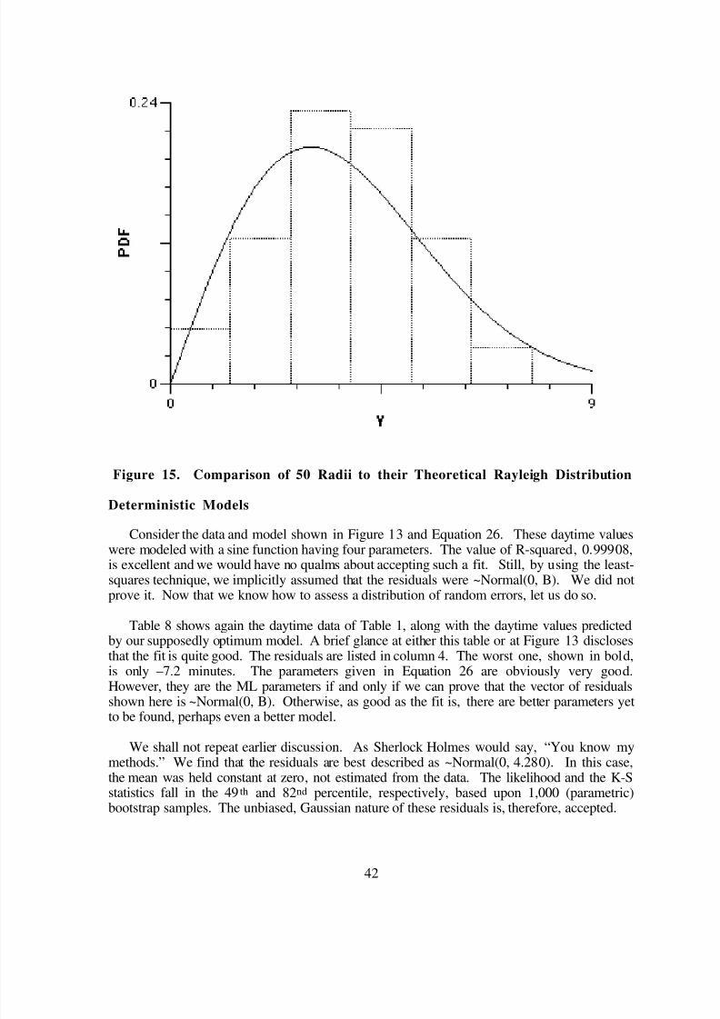
8/14/2019 Tutorial Math Modeling
http://slidepdf.com/reader/full/tutorial-math-modeling 46/54
42
Figure 15. Comparison of 50 Radii to their Theoretical Rayleigh Distribution
Deterministic Models
Consider the data and model shown in Figure 13 and Equation 26. These daytime valueswere modeled with a sine function having four parameters. The value of R-squared, 0.99908,is excellent and we would have no qualms about accepting such a fit. Still, by using the least-squares technique, we implicitly assumed that the residuals were ~Normal(0, B). We did notprove it. Now that we know how to assess a distribution of random errors, let us do so.
Table 8 shows again the daytime data of Table 1, along with the daytime values predictedby our supposedly optimum model. A brief glance at either this table or at Figure 13 disclosesthat the fit is quite good. The residuals are listed in column 4. The worst one, shown in bold,is only –7.2 minutes. The parameters given in Equation 26 are obviously very good.However, they are the ML parameters if and only if we can prove that the vector of residualsshown here is ~Normal(0, B). Otherwise, as good as the fit is, there are better parameters yet
to be found, perhaps even a better model.
We shall not repeat earlier discussion. As Sherlock Holmes would say, “You know mymethods.” We find that the residuals are best described as ~Normal(0, 4.280). In this case,the mean was held constant at zero, not estimated from the data. The likelihood and the K-Sstatistics fall in the 49th and 82nd percentile, respectively, based upon 1,000 (parametric)bootstrap samples. The unbiased, Gaussian nature of these residuals is, therefore, accepted.
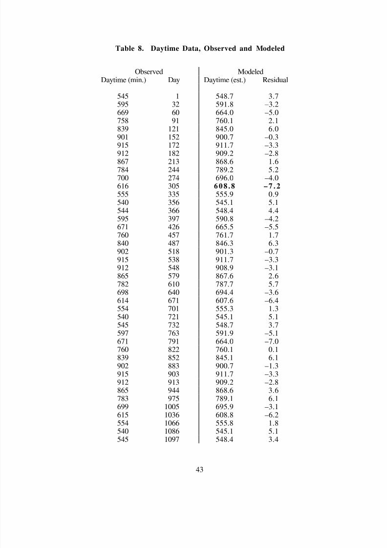
8/14/2019 Tutorial Math Modeling
http://slidepdf.com/reader/full/tutorial-math-modeling 47/54
43
Table 8. Daytime Data, Observed and Modeled
Observed ModeledDaytime (min.) Day Daytime (est.) Residual
545 1 548.7 3.7595 32 591.8 –3.2669 60 664.0 –5.0758 91 760.1 2.1839 121 845.0 6.0901 152 900.7 –0.3915 172 911.7 –3.3912 182 909.2 –2.8867 213 868.6 1.6784 244 789.2 5.2700 274 696.0 –4.0616 305 6 08 .8 – 7 . 2
555 335 555.9 0.9540 356 545.1 5.1544 366 548.4 4.4595 397 590.8 –4.2671 426 665.5 –5.5760 457 761.7 1.7840 487 846.3 6.3902 518 901.3 –0.7915 538 911.7 –3.3912 548 908.9 –3.1865 579 867.6 2.6
782 610 787.7 5.7698 640 694.4 –3.6614 671 607.6 –6.4554 701 555.3 1.3540 721 545.1 5.1545 732 548.7 3.7597 763 591.9 –5.1671 791 664.0 –7.0760 822 760.1 0.1839 852 845.1 6.1902 883 900.7 –1.3915 903 911.7 –3.3
912 913 909.2 –2.8865 944 868.6 3.6783 975 789.1 6.1699 1005 695.9 –3.1615 1036 608.8 –6.2554 1066 555.8 1.8540 1086 545.1 5.1545 1097 548.4 3.4
8/14/2019 Tutorial Math Modeling
http://slidepdf.com/reader/full/tutorial-math-modeling 48/54
44
In saying this, we imply only that the residuals, collectively, could easily have come from azero-mean Normal distribution. “Collectively” signifies that we do not consider the order of the residuals with respect to each other. If you look carefully at Table 8, column 4, you willnotice a suspicious alternation of positive and negative residuals. Such a periodicity would notbe observed in a random sample from any Gaussian distribution. It is, rather, a systematicerror in our model. It appears that we have not, after all, completely characterized the motions
of the Earth and Sun with this simple equation. Kepler could have told us that!
We forego perfection for the moment and take up the matter of uncertainty in the least-squares parameters. To do this, we shall again require a large number of nonparametricbootstrap samples. There are two common methods for obtaining such samples. We couldsimply resample the data points as we did with the 50 radii of the previous example. However,it is more common to use all of the data points and resample the residuals instead. If the latterare independent (hence, uncorrelated), then any residual might have been found associated withany data point. Here, there is some small amount of correlation but, for the sake of thisillustration, we shall ignore it and proceed in the usual fashion, using 1,000 bootstrap samples.
Doing so, we obtain simultaneous confidence intervals for all of the parameters, as follows:
A 90% --> [182.247, 184.318] (cf. Eq. 26, page 37)95% --> [181.944, 184.594]99% --> [181.354, 184.991]
B 90% --> [0.00273247, 0.00273958]95% --> [0.00273152, 0.00274036]99% --> [0.00272935, 0.00274223]
C 90% --> [–1.40549, –1.37757]95% --> [–1.40857, –1.37274]
99% --> [–1.41479, –1.36706]
D 90% --> [727.679, 729.264]95% --> [727.465, 729.569]99% --> [727.030, 729.939]
Note that the widths of these intervals, relative to parameter magnitude, are much narrower(i.e., better) than those seen in the example of the 50 random radii in spite of the fact that thelatter were a genuine sample from a known parent population while the sine model here isknown to be deficient.
It is difficult to predict the variability of parameters. It was not obvious, for instance, that
the uncertainty in the period of these data would be less than the uncertainty in the amplitude.Unless confidence intervals can be computed from theory, only a large bootstrap sample willyield this sort of information.
The interpretation of the confidence intervals is the same with these deterministic data as itwas with the stochastic data in the previous example. Also, the accuracy of the intervals willimprove, ceteris paribus, with bootstrap sample size.
8/14/2019 Tutorial Math Modeling
http://slidepdf.com/reader/full/tutorial-math-modeling 49/54
45
Parameter Correlation
There is one, final comment to make concerning confidence intervals and that concernstheir appearance. A confidence interval is just a range of numbers and it is very easy to fall intothe trap of believing that all of the numbers in that range are equally probable or, if there ismore than one such range for a given model, that any parameter may have any value in the
stated range regardless of the values of the other parameters. Neither of these beliefs is valid.
As an illustration, let us examine the nonparametric bootstrap results for the daytime datamore closely. Given 1,000 bootstrap samples, we may compute the mean of all the bootstrapparameters and, also, the covariance matrix.
The means are as follows:
A = 183.383B = 0.00273601C = –1.39028D = 728.435
Note, first of all, that these means are not quite equal to the ML values of the parameters.Bootstrap distributions are often unsymmetrical, with the mode and mean unequal.
Here is the upper triangle32 of the covariance matrix, with indices from A to D:
6.82581e–01 2.12136e–08 1.06586e–03 5.41600e–028.03571e–12 –2.29840e–08 4.54181e–07
1.19938e–04 –6.43826e–044.14830e–01
The ijth
entry in this matrix is given by Equation 28:
Cov Pij ≡ σ ij
2 = Pi – Pi P j – P j 28.
where P is a parameter.
When i = j, this is just the variance of parameter[j]; when i ≠ j, it is the covariance. As we
have seen before, the variance measures the intrinsic variability of P. The covariance measuresthe variability of one parameter with respect to another. Looking at this matrix, we see thatparameter B, the period, has the smallest variance. No matter what the other parameters might
have been, for any of the 1,000 bootstrap samples, the period stayed almost constant.
The sign of the covariance is an indication of the sense of correlation. Covariances that arepositive indicate that the two parameters in question increased and decreased together, onaverage. Negative covariances mean that, on average, one parameter increased when the otherdecreased. Here, for example, the amplitude of the sine wave, A, is positively correlated with 32 All covariance matrices are symmetric about the main diagonal.

8/14/2019 Tutorial Math Modeling
http://slidepdf.com/reader/full/tutorial-math-modeling 50/54
46
all of the remaining parameters. However, the phase, C, is negatively correlated with D. Toget an idea of how strong these relationships are, it is, perhaps, best simply to compare thecovariances for any parameter to its own variance. Any statistics textbook will discuss thesematters in great detail.
In any case, the implications with regard to confidence intervals is clear:
All combinations of parameters are not equally probable.
Summary
Our goal was to establish a quantitative measure of the variability of model parameters. Wehave succeeded by taking advantage of the power of the nonparametric bootstrap. The measureof variability obtained is a confidence interval which denotes the numerical range wherein thetrue value of the parameter is likely to be found with some specified probability. By usinginformation from the covariance matrix, we gain additional insight into the manner in whichparameters change with respect to each other when the dataset changes.

8/14/2019 Tutorial Math Modeling
http://slidepdf.com/reader/full/tutorial-math-modeling 51/54
47
99.9999999999% PERFECT!
The Rydberg constant describes the colors of atoms. For a hypothetical atom of infinitemass, its limiting value, R∞ = 109,737.3156864 cm–1, has an accuracy of more than twelve
significant figures [UDE97]. Think about that for a moment.
That’s like measuring the average distance between Earth and the Moon with an error lessthan the width of the period at the end of this sentence. Clearly, this is far beyond our currenttechnology. How, then, can we measure R∞ with such perfection?
Kepler, and his eponymous laws of planetary motion are partly responsible. Using thefirst and third of these, it is possible to derive the classical expression for the energy of anelectron in an atom. If this expression is combined with the laws of Quantum Mechanics (QM)and its insistence upon the importance of integers, the result is that an atom cannot have justany color but only a limited (yet still infinite!) set of colors.
Evidence for this conclusion can be illustrated using Hydrogen, the simplest atom, with the
simplest set of colors. The primary colors of Hydrogen are listed in Table 9.33
Table 9. Observed Transitions/Colors for Hydrogen (1H1)
Wavelength (in Angstroms)Nl 1 2 3 4 5 6
Series Lyman Balmer Paschen Brackett Pfund HumphriesNu Ultraviolet Visible Infra-red 2 1215.67 6562.72 18751.0 40511.6 74578.0 123685.3 1025.72 4861.33 12818.1 26251.5 46525.14 972.54 4340.47 10938.1 21655.3
5 949.74 4101.74 10049.46 937.80 3970.07 9546.07 930.75 3889.058 926.23 3835.389 923.15 3797.90
The Rydberg constant describes all of these colors via the model given in Equation 29.
Transition energy ~ RH1
N l2
– 1Nu
2 29.
where Nl and Nu are positive integers and where ~, in this case, means “is proportional to.”
According to the laws of QM, the color, i.e., the wavelength (λ) of the light emitted during
any transition is inversely proportional to its energy. The final model, based on these laws, isgiven by Equation 30. Fitting the data in Table 9 to Equation 30, the (unweighted) least-
33 see file Examples:Rydberg.in [WEA75]
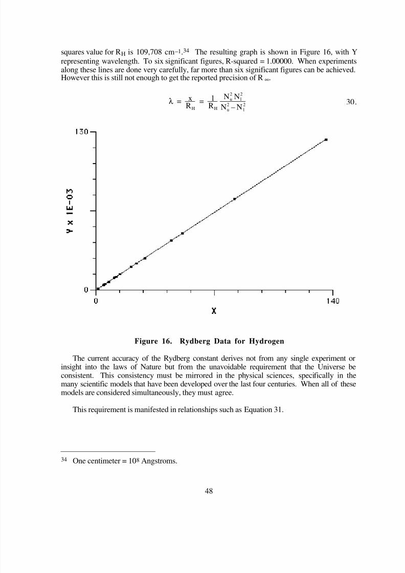
8/14/2019 Tutorial Math Modeling
http://slidepdf.com/reader/full/tutorial-math-modeling 52/54
48
squares value for RH is 109,708 cm–1.34 The resulting graph is shown in Figure 16, with Y
representing wavelength. To six significant figures, R-squared = 1.00000. When experimentsalong these lines are done very carefully, far more than six significant figures can be achieved.However this is still not enough to get the reported precision of R∞.
λ = xRH= 1RH
Nu
2
N l
2
Nu2 – N l
2 30.
Figure 16. Rydberg Data for Hydrogen
The current accuracy of the Rydberg constant derives not from any single experiment orinsight into the laws of Nature but from the unavoidable requirement that the Universe beconsistent. This consistency must be mirrored in the physical sciences, specifically in themany scientific models that have been developed over the last four centuries. When all of thesemodels are considered simultaneously, they must agree.
This requirement is manifested in relationships such as Equation 31.
34 One centimeter = 108 Angstroms.
8/14/2019 Tutorial Math Modeling
http://slidepdf.com/reader/full/tutorial-math-modeling 53/54
49
R∞ =2 π2 m e 4
c h3 31.
where m and e are the mass and charge of the electron, respectively, c is the speed of light, andh is Planck’s constant, the proportionality constant connecting energy to wavelength.
Equation 30 relates a mass, a charge, the speed of light, and several other constants, to theobservable colors of atoms. One can perform a variety of experiments to determine this mass,charge, or speed. In every case, there are still more factors, determinable in yet different ways.Each of these experiments depends upon a model and all of these models interlock. They arelike words in a crossword puzzle. The total solution will break down if even one of them isincorrect.
The physical sciences, which seek this total solution, are not incorrect; they are mature andreliable. One need only turn on a television set or view a CAT scan to appreciate that the lawsof the Universe are very well understood. Except at the frontiers of knowledge, the puzzle allholds together. It does not break down.
It is, in part, this internal consistency which affords the degree of accuracy that is seen inR∞. Whenever any physical experiment is performed, it yields a quantitative answer with some
precision. If sufficient attention has been paid to eliminating sources of error, the experimentwill have high precision. When many such experiments are incorporated into a single analysis,it is possible to compute a vector of means for any quantities, such as those in Equation 30,that their answers might have in common. As we have seen, in Equation 24 for instance, thesemeans will be more precise than any single experimental result. Simply put, the informationfrom many experiments necessarily exceeds the information provided by just one of them.
In our efforts at modeling, we have sought to extract information from data. The examplesdescribed herein illustrate that contemporary methodology is very effective in this task. When
the same methodology is applied to a collection of experiments, it is possible to achieve enoughsynergy to eliminate almost all of the residual error. It is possible to obtain 99.9999999999percent accuracy.
Twelve significant figures do not come about by accident. The techniques described in thistutorial are just the latest in a heritage that goes all the way back to Kepler and Galileo. Thatheritage is one which affirms the primacy of data as well as the power of mathematics andstatistics. These affirmations are implemented in techniques that are based upon the concept of maximum likelihood, techniques that literally construct the best possible match between theoryand experiment, between model and data.
In computing the optimum result, these same techniques explicitly acknowledge the role of
measurement error and sampling error. Even the best measurements are not perfect. Even thebest experiments must examine less than the entire Universe.
Error implies that the models we construct, and their parameters, must always be somewhatuncertain, however much we might like to believe otherwise. No model is complete until thoseuncertainties have been rigorously quantified. A good model knows its limitations…

8/14/2019 Tutorial Math Modeling
http://slidepdf.com/reader/full/tutorial-math-modeling 54/54
…as does a good tutorial.
We began with data, but where do we end? Perhaps T. S. Eliot had the right idea:
“We shall not cease from explorationAnd the end of all our exploring
Will be to arrive where we startedAnd know the place for the first time.”
And be ready to start again on a new adventure, older and wiser, and better prepared—
to experiment,
to analyze,
to play the game one more time.