Tutorial lecture, QFS&MBTNiagara Falls, NY, USA, 15.8.2015

Introduction to Landau’s Fermi Liquid Theory

Erkki Thuneberg

Department of physics

University of Oulu

1. IntroductionThe principal problem of physics is to determine how

bodies behave when they interact. Most basic courses ofclassical and quantum mechanics treat the problem of oneor two particles or bodies. (An external potential can beconsidered as one very heavy body.) The problem gets mo-re difficult when the number of bodies involved is larger.In particular, in condensed matter we are dealing with amacroscopic number N ∼ 1023 of particles, and typicallyhundreds of them directly interact with each other. Thisproblem is commonly known as the many-body problem.

There is no general solution to the many-body problem.Instead there is a great number of approximations thatsuccessfully explain various limiting cases. Here we discussone of them, the Fermi-liquid theory. This type of approxi-mation for a fermion many-body problem was invented byLandau (1957). It was originally proposed for liquid 3Heat very low temperatures. Soon it was realized that a simi-lar approach could be used to other fermion systems, mostnotably to the conduction electrons of metals. The Fermi-liquid theory allows to understand very many propertiesof metals. A generalization of the Fermi-liquid theory al-so allows to understand the superconducting state, whichoccurs in many metals at low temperatures. Even whenLandau’s theory is not valid, it forms the standard againstwhich to compare more sophisticated theories. Thus Fermi-liquid theory is a paradigm of many-body theories, and itis presented in detail in many books and articles discussingthe many-body problem.

• L.D. Landau and E.M. Lifshitz, Statistical Physics,Part 2 (Pergamon, Oxford, 1980).

• P. Nozieres, Theory of interacting Fermi systems (Be-jamin, New York 1964) [N].

• D. Pines and P. Nozieres, The theory of quantumliquids, Vol. 1 Normal Fermi liquids (Bejamin, NewYork 1966).

• G. Baym and C. Pethick, Landau Fermi-liquid theory(Wiley, Ney York 1991) [BP].

• A.A. Abrikosov and I.M. Khalatnikov, Rep. Progr.Phys. 22, 329 (1959), an early review.

• A.J. Leggett, Rev. Mod. Phys. 47, 331 (1975), andQuantum liquids (Oxford, 2006).

In this lecture I present an introduction to the Landautheory. I present the theory as if it could have logicallydeveloped, but this does not necessarily reflect historicalfacts. I will start with the calculation of specific heat in anideal gas, and compare the result with the measurementin liquid 3He. This leads to the concept of quasiparticleswith an effective mass differing from the atomic mass. Itis then shown that in order to make a consistent theory,one has to allow an interaction between the quasiparticles.After having formulated the theory, we shortly mention themain applications. Some more recent results are discussed

in more length. Various generalizations of the theory arebriefly mentioned.

1

2. Preliminary topics

Many-body problem

The many-body problem for identical particles can beformulated as follows. Consider particles of mass m labeledby index i = 1, 2, . . . , N . Their locations and momenta arewritten as rk and pk. The Hamiltonian is

H =

N∑k=1

p2k

2m+ V (r1, r2, . . .). (1)

Here V describes interactions between any particles, andit could in many cases be written as a sum of pairwiseinteractions V = V12 + V13 + . . .+ V23 + . . .. The classicalmany-body problem is to solve the Newton’s equations.

In quantum mechanics the locations and momenta beco-me operators. In the Schrodinger picture pk → −ih∇k,where

∇k = x∂

∂xk+ y

∂

∂yk+ z

∂

∂zk. (2)

An additional feature is that generally particles have spin.This is described by an additional index σ that takes values−s,−s + 1, . . . , s − 1, s for a particle of spin s. Thus theHamiltonian operator is

H = −N∑k=1

h2

2m∇2k + V (r1, σ1, r2, σ2, . . .). (3)

and the state of the system is described by a wave func-tion Ψ(r1, σ1, r2, σ2, . . . ; t). Particles having integral spinare called bosons. Their wave function has to be symmet-ric in the exchange of any pairs of arguments. For example

Ψ(r1, σ1, r2, σ2, r3, σ3, r4, σ4, . . .)

= +Ψ(r3, σ3, r2, σ2, r1, σ1, r4, σ4, . . .), (4)

where coordinates 1 and 3 have been exchanged. Particleshaving half-integral spin are called fermions. Their wavefunction has to be anti-symmetric in the exchange of anypairs of arguments. For example

Ψ(r1, σ1, r2, σ2, r3, σ3, r4, σ4, . . .)

= −Ψ(r3, σ3, r2, σ2, r1, σ1, r4, σ4, . . .). (5)

The quantum many body problem is to solve time-dependent Schrodinger equation

ih∂Ψ

∂t(r1, σ1, . . . , rN , σN , t) = HΨ(r1, σ1, . . . , rN , σN , t)

(6)or to solve energy eigenvalues and eigenstates.

Ideal Fermi gas

As stated in the introduction, there is no general solutionof the many-body problem. What one can do is to studysome limiting cases. One particularly simple case is ideal

gas, where we assume no interactions, V ≡ 0. Below weconcentrate on ideal spin-half (s = 1/2) Fermi gas.

In the absence of interactions we can assume a facto-rizable form

Ψ0(r1, σ1, r2, σ2, . . . ; t) = φa(r1, σ1)φb(r2, σ2) . . . . (7)

consisting of a product of single-particle wave functionsφα(r, σ). This does not yet satisfy the antisymmetry requi-rement (5) but permuting the arguments in Ψ0 and sum-ming them all together multiplied by (−1)nP , where nP isthe number of pairwise permutations in a permutation P ,one can generate a proper wave function

Ψ(r1, σ1, r2, σ2, . . .) =1√N

∑P

(−1)nP

×φa(rP (1), σP (1))φb(rP (2), σP (2))) . . . . (8)

This is known as Slater determinant since it can also bepresented as a determinant

Ψ =1√N

∣∣∣∣∣∣∣φa(r1, σ1) φb(r1, σ1) . . .φa(r2, σ2) φb(r2, σ2) . . .

......

. . .

∣∣∣∣∣∣∣ . (9)

We can now see if any two of the single-particle wavefunctions φa, φb, . . . are identical, the resulting wave func-tion vanishes identically. (Verify this in the case of two fer-mions.) This is the Pauli exclusion principle, which statesthat a single state can be occupied by one fermion only.

The natural choice for wave functions of a single freeparticle are plane wave states. In order to incorporate thespin, we have “spin-up states”

φp↑(r, σ) =

1√Veip·r/h if σ = 1

2

0 if σ = − 12

(10)

and “spin-down states”

φp↓(r, σ) =

0 if σ = 1

21√Veip·r/h if σ = − 1

2

. (11)

Here the wave vector k or the momentum p = hk appearsas a parameter. In order to count the states, it is mostsimple to require that the wave functions are periodic in acube of volume V = L3, which allows the momenta p (jx,jy and jz are integers)

px =2πhjxL

, py =2πhjyL

, pz =2πhjzL

. (12)

We suppose that the volume V is very large. Then we cantake the limit V →∞ in quantities that do not essentiallydepend on V .

The energy of a single-particle states is εp = p2/2m. Thetotal energy is this summed over all occupied states

E(npσ) =∑σ

∑p

p2

2mnpσ, (13)

2

where npσ = 1 for an occupied state and is zero otherwise.

The ground state of a system with N particles has Nlowest energy single-particle states occupied and othersempty. Here the maximal kinetic energy of an occupiedstate is called Fermi energy εF . We also define the Fermiwave vector kF and Fermi momentum pF = hkF so that

εF =p2F

2m=h2k2

F

2m. (14)

In momentum space this defines the Fermi surface (p =pF ). All states inside the Fermi surface (p < pF ) are occu-pied, and the ones outside are empty.

× × × × × × × × × × × × × ×× × × × × × × × × × × × × ×× × × × × × × × × × × × × ×× × × × × × × × × × × × × ×× × × × × × × × × × × × × ×× × × × × × × × × × × × × ×× × × × × × × × × × × × × ×

× × × × × × × × × × × × × ×× × × × × × × × × × × × × ×× × × × × × × × × × × × × ×× × × × × × × × × × × × × ×× × × × × × × × × × × × × ×× × × × × × × × × × × × × ×× × × × × × × × × × × × × ×

px

-

pF

2πhL

py

××××××××

×××××××

× × × × × × × × × × × × × ×

The number of particles can be calculated as

N = 2∑p<pF

1 = 243πp

3F

(2πh/L)3, (15)

where the factor 2 comes from spin. From this we get arelation between the Fermi wave vector and the particledensity,

N

V=

p3F

3π2h3 . (16)

The excited states of the system consist of states whereone or more fermions is excited to higher energy states. Theaverage occupations of the states at a given temperatureT is given by the Fermi-Dirac distribution

n(ε) =1

eβ(ε−µ) + 1. (17)

Here β = 1/kBT and kB = 1.38×10−23 J/K is Boltzmann’sconstant, which is needed to express the temperature T inKelvins, and µ is the chemical potential. At T = 0 thesystem is in its ground state,

n(ε) =

1 for ε < µ0 for ε > µ.

(18)

with µ = εF . When T > 0, the occupation n(ε) gets roun-ded so that the change from n ≈ 1 to n ≈ 0 takes place inthe energy interval ≈ kBT .

ε

n T = 0

T > 0

0 εF

kBT

Next we calculate the specific heat of the ideal Fermi gasat low temperatures. The average energy is given by

E =∑σ

∑p

εpn(εp) =2

(2πh/L)3

∫εpn(εp)d

3p

=8π

(2πh/L)3

∫ ∞0

p2εpn(εp)dp. (19)

Changing ε = p2/2m as the integration variable we get

E

V=

√2m3

π2h3

∫ ∞0

ε3/2n(ε)dε

=

∫ ∞0

g(ε)ε n(ε)dε. (20)

In the second line we have expressed the same result bydefining a density of states g(ε) = m

√2mε/π2h3.

The specific heat is now obtained as the derivative ofenergy

C =∂E(T, V,N)

∂T. (21)

In order eliminate µ appearing in the distribution function(17) one has to simultaneously satisfy

N

V=

∫ ∞0

g(ε)n(ε)dε. (22)

The result calculated with Mathematica is shown below.

0.0 0.5 1.0 1.5 2.0

T

TF

0.2

0.4

0.6

0.8

1.0

2 C

3 N kB

At high temperatures T TF = εF /kB the Fermi gasbehaves like classical gas, where the average energy perparticle is 3kBT/2, known as the equipartition theorem,and this gives the specific heat 3kB/2 per particle. We seethat at lower temperatures T < TF the specific heat isreduced. This can be understood that only the particleswith energies close to the Fermi surface can be excited.Those further than energy kBT from the Fermi surfacecannot be excited, and thus do not contribute to specificheat. At temperatures T TF the specific heat is linearin T :

C =π2

3g(εF )k2

BT +O(T 2). (23)

We see that the linear term is determined by the densityof states at the Fermi surface

g(εF ) =mpF

π2h3 . (24)

3

(For detailed derivation see Ashcroft-Mermin, Solid statephysics.)

Liquid 3He

Helium has two stable isotopes, 4He and 3He. The formeris by far more common in naturally occurring helium. It isa boson since in the ground state both the two electronshave total spin zero, and also the nuclear spin is zero. It hasa lot of interesting properties that could be discussed, buthere we concentrate on the other isotope. 3He is a fermionbecause the nuclear spin is one half, s = 1/2. Studies of 3Hewere started as it became available in larger quantities inthe nuclear age after world war II as the decay product oftritium. The two isotopes of helium are the only substancesthat remain liquid even at the absolute zero of temperature.

Figure: the specific heat of liquid 3He at two differentdensities [D.S. Greywall, Phys. Rev. B 27, 2747 (1983)].

We see that at low temperatures, the specific heat is li-near in temperature. This resembles the ideal gas discussedabove, but is quite puzzling since the atoms in a liquid aremore like hard balls continuously touching each other!

Also, quantitative comparison of the slope with the idealFermi gas gives that the measured slope is by factor 2.7larger.

3. Construction of the theory

Landau’s idea

The experiment above raises the following idea. Could itbe possible that low temperature liquid 3He would effec-tively be like an ideal gas? This was the problem Landaustarted thinking. He had to answer the following questions

• How could dense helium atoms behave like an idealgas?

• If there is explanation to the first question, how onecan understand the difference by 2.7 in the density ofstates?

• If previous questions have positive answers, are anyother modifications needed compared to the ideal gas?

An obvious problem with the ideal gas wave function (8)is that there is too little correlation between the locationsrk of the particles. The Pauli principle prohibits for twoparticles with the same spin to occupy the same location,but there is no such restriction for particles with oppositespins. Thus it is equally likely to find two opposite-spinparticles just at the same place than at any other places inthe ideal gas wave function (8).

Weak interactions

As a first attempt to answer the questions, considerpoint-like particles (instead of real 3He atoms). In an idealgas the particles fly straight trajectories without ever col-liding. If we now allow some small size for the particles,they will collide with each other.

r00

U(r)ac

db

Figure: illustration of various particle-particle potentialsU(r): (a) the potential between two 3He atoms, (b) idealgas potential U ≡ 0, (c) potential used in scattering ap-proach, (d) potential used in perturbation theory.

We have to consider two particles with momenta p1 andp2 colliding and leaving with momenta p′1 and p′2. In sucha process the momentum and energy has to be conserved,

p1 + p2 = p′1 + p′2 (25)

ε1 + ε2 = ε′1 + ε′2. (26)

At least qualitatively the collision rate can be calculatedusing the golden rule

Γ =2π

h

∑f

|〈f |Hint|i〉|2δ(Ef − Ei). (27)

4

We see that the rate is proportional to the number of avai-lable final states f . Consider specifically the case of filledFermi sphere plus one particle at energy ε1 > εF . We wishto estimate the allowed final states when particle 1 collideswith any particle inside the Fermi sphere, ε2 < εF . Thefinal state has to have two particles outside the Fermi sp-here (ε′1 > εF , ε′2 > εF ) since the Pauli principle forbids allstates inside. We see that the number final states gets verysmall when the initial particle is close to the Fermi energy,namely both ε2 and ε′1 have to be chosen in an energy shellof thickness ∝ ε1− εF . This means that the final states arelimited by factor ∝ (ε1 − εF )2. Thus the scattering of lowenergy particles is indeed suppressed and thus resemblesthe one in an ideal gas.

But 3He atoms are not point particles, rather they toucheach other continuously. Thus for one particle to move,the others must give the way. This is one of the hardestproblems in many body theory even today, but one canget some idea of what happens with a model: instead oftrue 3He-3He interaction potential, one assumes a weakpotential, whose effect can be calculated using quantum-mechanical perturbation theory. We will skip this calcula-tion here (see Landau-Lifshitz). The result is that the exci-tation spectrum remains qualitatively similar as in free Fer-mi gas but there is a shift in energies. Consider specificallythe case, already mentioned above, of a filled Fermi sphe-re plus one particle at momentum p, with p > pF . Thisexcited state of the ideal gas corresponds to the excitationenergy

εp − εF =p2

2m− εF ≈

pFm

(p− pF ), (28)

where the approximation is good if p is not far from theFermi surface (p− pF pF ). The effect of the weak inte-ractions is now that the excitation energy still is linear inp−pF , but the coefficient is no more pF /m. It is customaryto write the new excitation energy in the form

εp − εF =pFm∗

(p− pF ), (29)

where we have defined the effective mass m∗. Note thatthe Fermi momentum pF is not changed, equation (16)still remains valid. With the new dispersion relation (29)we get a new density of states

g(εF ) =m∗pF

π2h3 . (30)

This is determined by the effective mass m∗, not the ba-re particle mass m as for ideal gas (24). We now see thatweak interactions can explain that the specific heat coef-ficient (23) differs from its ideal gas value. However, thetheory is valid for small perturbations, say 10%, and thusis insufficient to explain the factor 2.7.

Quasiparticles

Landau now made the following assumptions. i) Even forstrong interactions, the excitation spectrum remains as in

(29). Such excitations are called quasiparticles: they deve-lop continuously from single-particle excitations when theinteractions are ”turned on”, but they consist of correlatedmotion of the whole liquid. ii) The quasiparticles have longlife time at low energy, like in the scattering approximationabove.

It should be noticed that Landau’s theory is phenome-nological. At this stage it has one parameter, m∗, whosevalue is unknown theoretically, but can be obtained fromexperiments.

Although the detailed structure of the quasiparticle re-mained undetermined, we can develop a qualitative pic-ture with a model. Consider a spherical object moving inotherwise stationary liquid. The details of this model arediscussed in the appendix. The main result is that associa-ted with the moving object, there is momentum in the fluidin the same direction. In the literature this is sometimescalled ”back flow”, but I find this name misleading. Rat-her it should be called ”forward flow”or that the movingobject drags with itself part of the surrounding fluid. Thin-king now that the total momentum of the quasiparticle isfixed, this means that switching on the interactions slowsthe original fermion down, since part of the momentumgoes into the surrounding fluid and less is left for the ori-ginal fermion.

The same picture is obtained by quantum mechanicalanalysis. In order to get the velocity of the quasiparticle,we have to form a localized wave packet. This travels withthe group velocity. Based on the dispersion relation (29)the group velocity is

vgroup =dEpdp

=pFm∗

. (31)

This means that the momentum of the original fermion inthe interacting system is mvgroupp = (m/m∗)p, i.e. theoriginal fermion contributes fraction m/m∗ of the momen-tum p and the fraction 1−m/m∗ is contributed by otherfermions surrounding the original one. The velocity of thequasiparticle (31) is known as the Fermi velocity

vF =pFm∗

. (32)

Quasiparticle interactions

Thus far we have arrived at the picture that the lowenergy properties of a Fermi liquid can be understood asan ideal gas with the difference that the effective mass m∗

5

appears instead of the particle mass m. In the followingwe show that this cannot be the whole story, and one moreingredient has to be added in order to arrive at a consistenttheory.

A general requirement of any physical theory is that thepredictions of the theory should be independent of the coor-dinate system chosen. In the present case, one has to payattention to Galilean invariance. That means that the phy-sics should be the same in two coordinate frames that mo-ve at constant velocity with respect to each other. To bespecific consider a coordinate system O, and a second coor-dinate system O′ that moves with velocity u as seen in theframe O. We assume to study a system of N particles (in-teracting or not) of mass m. If the total momentum of thissystem in O′ is P ′, then the momentum seen in frame Ohas to be P = P ′ + Nmu. Now the Galilean invariancerequires that if one determines the state of the system inO′ at fixed total momentum P ′, it is the same as one woulddo in O with momentum P .

The ideal gas obviously satisfies Galilean invariance.However, when we replace the particle mass m by m∗ in(29), the Galilean invariance is broken. The cure for thisproblem is that we have to allow interactions between thequasiparticles. Thus we rewrite (29) into the form

εp − εF =pFm∗

(p− pF ) + δεp, (33)

δεp =1

V

∑σ

∑p′

f(p,p′)(np′ − n(0)p′ ). (34)

Here np is the distribution of the quasiparticles, n(0)p =

Θ(pF − p) is the distribution function in the ground sta-te, where Θ(x) is the step function (Θ(x) = 0 for x < 0and Θ(x) = 1 for x > 0). The function f(p,p′) describesthe interaction energy between two quasiparticles havingmomenta p and p′.

The first thing to notice is that when only one or a fewquasiparticles are excited, the interaction term in (34) is

negligible since np − n(0)p ≈ 0. In this case the excitation

energy εp (34) reduces to its the previous expression (29).

Consider next an uniformly displaced Fermi sphere, np =

n(0)p−mu = Θ(pF − |p−mu|). This is the stationary ground

state in the O′ frame. In order to the theory to be Galileaninvariant, the excitation energy must be changed from (29)to the ideal gas value (28) at the displaced Fermi surface.As a formula

pFmmp ·u =

pFm∗

mp ·u+1

V

∑σ

∑p′

f(p,p′)(n(0)p′−mu−n

(0)p′ ).

(35)We see that this could not be satisfied without the interac-tion term. In order to work (35) further, we need to studyf(p,p′). Because of spherical symmetry, it can depend on-ly on the relative directions of p and p′, i.e. f(p · p′, p, p′).Futher since we are interested only in quasiparticles clo-se to the Fermi surface, we approximate f(p · p′, p, p′) ≈f(p · p′, pF , pF ). This means that f depends only on theangle between p and p′, i.e. f(p · p′). In addition, it is

conventional to define F (p · p′) = g(εF )f(p · p′). Such afunction can be expanded in Legendre polynomials

F (p · p′) =

∞∑l=0

F sl Pl(p · p′), (36)

where P0(x) = 1, P1(x) = x, P2(x) = (3x2 − 1)/2, etc.Using these we can now reduce the requirement (35) to

m∗

m= 1 +

F s13. (37)

We have arrived at the result that in order to havem∗ 6= m, we also should include an interaction betweenthe quasiparticles of the form of the F s1 term in (36). Theother interaction terms with coefficients F sl are not requi-red for internal consistency of the theory but some of themappear as a result of perturbation theory. In order to makegeneral phenomenology, they all should be retained.

Until now we have not considered the fermion spin exceptthat they produced factors of two. In magnetic field the sys-tem becomes spin polarized, and this is no more sufficient.In the general case we have to consider the spin as a fullyquantum object. This means that we have to replace npby a 2 × 2 density matrix in spin space. All the previousanalysis can be generalized to include the spin dependence.This means that also the quasiparticle energy εp becomesa 2× 2 matrix. Equation (33) has to be generalized to

εην(p)− εF δην =pFm∗

(p− pF )δην

+1

V

∑p′

∑α,β

fηα,νβ(p,p′)[nαβ(p′)− n(0)(p′)δαβ ], (38)

where

fηα,νβ(p,p′)

g(εF )=

∞∑l=0

(F sl δηαδνβ + F al σηα · σνβ)Pl(p · p′).

(39)We see that including the spin dependence the theory hastwo sets of parameters, F sl and F al with l = 0, 1, . . .. (Heres denotes symmetric and a antisymmetric.) One of theseparameters F s1 is related to m∗ by (37).

The expression for εp − εF (33) can be seen as the cons-tant and the first order term in the expansion of εp interms of distribution np. In applications these two termsgenerally are of the same order of magnitude even thoughthe deviation from ground state distribution is assumedsmall. The reason that they are of equal magnitude is thatthe first term in (33) vanishes at the Fermi surface p = pFwhereas the latter term remains finite. The situation re-sembles the one in another theory developed by Landau:the Ginzburg-Landau theory. There the free energy is ex-panded in the order parameter as F = α|ψ|2 + β|ψ|4. Alt-hough the latter term is small because of the higher powerin the small |ψ|, the two terms are comparable because thecoefficient α vanishes at the critical temperature whereasβ remains finite.

6

4. Equation of motionThe central quantity in the theory is the quasiparticle

distribution function np(r, t). Its equation of motion is de-rived similarly as the Boltzmann equation, by calculatingthe total time derivative

dnpdt

=∂np∂t

+ r ·∇np + p · ∂np∂p

=∂np∂t

+∂εp∂p·∇np −∇εp ·

∂np∂p

, (40)

where r ≡ dr/dt = ∂εp/∂p and p ≡ dp/dt = −∇εp.Equating this with the rate of change caused by collisionsIp gives the Landau-Boltzmann equation

∂np∂t

+∂εp∂p·∇np −∇εp ·

∂np∂p

= Ip. (41)

This differs from the ordinary Boltzmann equation thatthe energy εp(r, t) contains, in addition to external poten-tials, the interaction energy δεp (34). The collisions haveto conserve the fermion number, momentum and energy.This implies on the collision term the conditions∑

p

Ip = 0,∑p

pIp = 0,∑p

εpIp = 0. (42)

The kinetic equation equation (41) is a nonlinear equa-tion. For most, if not all, applications a linearized form ofit is sufficient. In equilibrium both ∇np and ∇εp vanish,and thus in a linearized theory their multipliers in (41) canbe evaluated in the equilibrium state. Thus linearization ofthe left hand side gives

∂np∂t

+ vFp ·∇(np −

dn(0)p

dεpδεp

)= Ip, (43)

where dn(0)p /dεp denotes the derivative of the equilibrium

distribution function (17) evaluated at the unperturbedenergy (29).

Once we have solved for the distribution functionnp(r, t), we can calculate measurable quantities. Forexample, the mass density and momentum density of thefluid are given by

ρ = ρ0 +m2

V

∑p

(np − n(0)p ), (44)

J =2

V

∑p

p (np − n(0)p ). (45)

Here the factors of 2 come from spin. The momentum den-sity is the same as the mass current density. Because ofconservation of mass and momentum, these have to obeyconservation laws

∂ρ

∂t+ ∇ · J = 0, (46)

∂J

∂t+ ∇ ·Π = 0, (47)

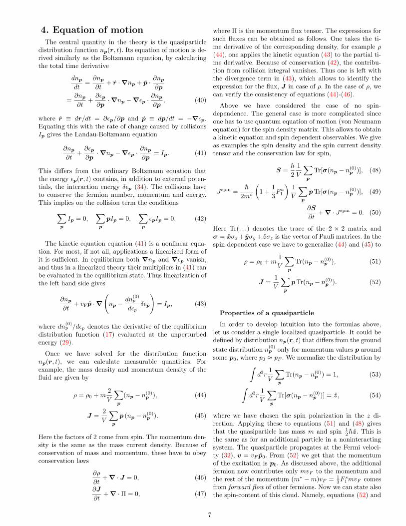
where Π is the momentum flux tensor. The expressions forsuch fluxes can be obtained as follows. One takes the ti-me derivative of the corresponding density, for example ρ(44), one applies the kinetic equation (43) to the partial ti-me derivative. Because of conservation (42), the contribu-tion from collision integral vanishes. Thus one is left withthe divergence term in (43), which allows to identify theexpression for the flux, J in case of ρ. In the case of ρ, wecan verify the consistency of equations (44)-(46).

Above we have considered the case of no spin-dependence. The general case is more complicated sinceone has to use quantum equation of motion (von Neumannequation) for the spin density matrix. This allows to obtaina kinetic equation and spin dependent observables. We giveas examples the spin density and the spin current densitytensor and the conservation law for spin,

S =h

2

1

V

∑p

Tr[σ(np − n(0)p )], (48)

J spin =h

2m∗

(1 +

1

3F a1

)1

V

∑p

pTr[σ(np − n(0)p )], (49)

∂S

∂t+ ∇ · J spin = 0. (50)

Here Tr(. . .) denotes the trace of the 2 × 2 matrix andσ = xσx+ yσy+ zσz is the vector of Pauli matrices. In thespin-dependent case we have to generalize (44) and (45) to

ρ = ρ0 +m1

V

∑p

Tr(np − n(0)p ), (51)

J =1

V

∑p

pTr(np − n(0)p ). (52)

Properties of a quasiparticle

In order to develop intuition into the formulas above,let us consider a single localized quasiparticle. It could bedefined by distribution np(r, t) that differs from the ground

state distribution n(0)p only for momentum values p around

some p0, where p0 ≈ pF . We normalize the distribution by∫d3r

1

V

∑p

Tr(np − n(0)p ) = 1, (53)∫

d3r1

V

∑p

Tr[σ(np − n(0)p )] = z, (54)

where we have chosen the spin polarization in the z di-rection. Applying these to equations (51) and (48) givesthat the quasiparticle has mass m and spin 1

2 hz. This isthe same as for an additional particle in a noninteractingsystem. The quasiparticle propagates at the Fermi veloci-ty (32), v = vF p0. From (52) we get that the momentumof the excitation is p0. As discussed above, the additionalfermion now contributes only mvF to the momentum andthe rest of the momentum (m∗ −m)vF = 1

3Fs1mvF comes

from forward flow of other fermions. Now we can state alsothe spin-content of this cloud. Namely, equations (52) and

7

(49) together imply that the effective number of spin upand spin down particles in the quasiparticle are

n↑ = 1 +1

6(F s1 + F a1 ), n↓ =

1

6(F s1 − F a1 ). (55)

That is, the total mass current in the quasiparticle carriedby spin-up particles is n↑mvF and correspondingly n↓mvFis carried by spin-down particles.

5. ApplicationsThe Fermi-liquid theory can be applied to calculate se-

veral measurable properties of a Fermi liquid. Below we listsome of them. The standard applications are only brieflymentioned as they can be found in most reviews of theFermi-liquid theory [see references mentioned in the intro-duction].

Specific heat. For a Fermi gas this was calculated in Eq.(23):

C =π2

3g(εF )k2

BT +O(T 2). (56)

The effect of interactions is that the density of states isgiven by the effective mass m∗ in (30).

Magnetic susceptibility. In magnetic field the Fermiliquid is spin-polarized. The magnetic susceptibility is

χ = µ0µ2m

g(εF )

1 + F a0, (57)

where µm is the magnetic moment of a particle. This resultdiffers from a Fermi gas by the presence of F a0 .

Sound velocity. An ordinary (longitudinal) sound wavecan propagate in a Fermi liquid. The velocity of the waveis

c = vF

√1

3(1 + F s0 )(1 +

1

3F s1 ). (58)

Once F s1 is extracted from measurement of the specificheat, measuring the sound velocity can give the value ofF s0 . In 3He F s0 ranges from 9 to 90 depending on pressure.The large value reflects the strong repulsion of the atomsupon compression.

Zero sound. Ordinary sound depends on collisions thatkeep the fluid elements in their local equilibrium state. Ina Fermi liquid the collisions get rare at low temperatures,which leads to strong damping of the ordinary sound. Anew type of propagating wave, called zero sound, can ap-pear at low temperatures. Depending on the interactionparameters, it can propagate in total absence of collisions.The velocity of the wave depends in a complicated wayon the interaction parameters. In 3He its velocity is ratherclose to the velocity of the ordinary sound because of thelarge value of F s0 .

8

VGLUMK 17, NUMBER 2 PHYSICAL REVIEW LETTERS 11JULY 1966

400—

I'

I'I

I I ltTI I

'I'I

I I IIII Table I. Values of the coefficients &0 and A~ of Eqs.(1) and (2) for several runs.

300—

200

Cd /27l AoRun (MHz) 106 (K 2 cm) ]

A([].0 sec K /c m]

EC3

I

I- IOO

à sogb 60OOz 400

3O

LLI 20I—

tLIC3

lo

8

196—

I I I I II 'I

T —MILLIDEGREES KELVIN

I94-C3

l92—I

I—

OO 190—

I88—

~0Cn t9~ ~ go000 00 oo0

0 00

oo o 0

08 0DCO 0 O OD0

Also important is the temperature Tmax*at which one finds maximum attenuation or max-imum rate of change with temperature of thevelocity. Under the simplest assumptions thistemperature corresponds to wT = 1, where vis the relaxation time for velocity, which isassumed to have a T ' temperature dependence.However, mare generally one would expect~'"/Tmax* to be a. constant at the maximum.Table II shows the results of an analysis ofthis point, both for the present experimentsand for those of Ref. 3. Inspection of the table

I86 I I iI I I IIII I I I I I IIII I

FIG. 2. Amplitude attenuation coefficient and soundpropagation velocity as a function of magnetic tempera-ture in pure liquid He3 at 0.32 atm and for frequenciesof 15.4 and 45.5 MHz. Each point shown on the graphis the average of several raw data points. The straightline drawn through the low-temperature attenuation da-ta represents Eq. (1), while the straight lines drawnthrough the high-temperature data represent Eq. (2),with u/27r equal to 15.4 and 45.5 MHz. With the presentgap it was not possible to measure the 45.5-MHz atten-uation coefficient above e =200 cm . The smoothcurve just above the attenuation data for 15.5 MHz is aplot of Eq. (6) with cd/27I =15.4 MHz and eo and 0.

& givenby Eqs. (1) and (2).

15.415.445.515.4

1.441.57l.581.62

2.742.652.662.65

shows that, in the case of attenuation measure-ments, in which Tmax* is well determined,the frequency dependence is quantitatively veri-fied. It is difficult to estimate Tm~ fromthe velocity measurements, so the scatter isgreater. However, it seems clear from thesedata that the transition observed in Ref. 3 isindeed to be attributed to a transition from firstto zero sound.Our results can also be compared with the

theory of Khalatnikov and Abrikosov' in whichthe velocity of zero sound is found to be givenby the implicit equation

1 + ,'E, —Eo(l +—,'E, ) + so'E, '

(4)

For the values given above for the parametersin Eq. (4), one finds T,T'=1.5xlp "secK".

where zo(s, ) =1(s,/2) ln[(s, +1)/(s, -l)]f-l, sp=cp/vF, and vF is the Fermi velocity. Recent-ly determined' values of the Fermi-liquid param-eters are Eo:10 77 +,:6 25 and vF:53 8m/sec for a pressure of 0.28 atm (close to thepresent one). At this pressure c, =187.2 m/sec.Solving Eq. (3) for s, one finds s, = 3.597 [andM (s,) = 0.027 033]. This leads to [(cp-cl )/cl]p 28 atm

——0.034, in remarkable agreementwith the measured value at 0.32 atm of 0.035+ 0.003. Using a theory for energy transferfrom a solid to liquid He', Keen, Matthews,and Wilks' found (c,-c,)/c, =0.10+0.03, a largereffect than observed here. Assuming the es-sential correctness both of the experirgentsof Ref. 3 and of the present ones, the discrep-ancy in the value of (co—c,)/c, must be attributedto an inadequacy of the theory explaining ener-gy transfer into the liquid.In regard to attenuation, at high temperatures

one expects'

[W.R. Abel, A.C. Anderson and J.C. Wheatley, Phys.Rev. Lett. 17, 74 (1966).]

Spin waves. Consider a local deviation of spin densityfrom its equilibrium value. In a Fermi gas this relaxes bydiffusion of the particles, called spin diffusion. In a Fermiliquid the interactions intervene so that instead of diffusion,propagating waves of spin density can be generated. Oneparticularly interesting case is the following. Consider sta-tic magnetic field H = Hz and the magnetization vectorM . For M+ = Mx + iMy we can write the equation

iD∇2M+ + ΩM+ = i∂M+

∂t. (59)

At high temperature D is real and this is a simple dif-fusion equation with an additional term −iΩM+ comingfrom precession at the Larmor frequency Ω = γH. At lowtemperature D is imaginary, and Eq. (59) becomes theSchrodinger equation, where Ω is the potential. Thus asa function of temperature one changes continuously from adissipative diffusion equation to a conservative wave equa-tion. The standing waves in a potential well caused by in-homogeneous H(r) nicely show up in the experiment byCandela et al [J. Low Temp. Phys. 63, 369 (1986)].

3 8 2 D . C a n d e l a , N . M a s u h a r a , D. S. Sherrili, and D. O. E d w a r d s

12.3 bar. (Some data at 3 bar can be found in ref. 21.) The data for p = 0 best satisfy the condition ]Im(D)] >> Re(D). This is because the superfluid transition temperature Tc increases rapidly with pressure. The maximum achievable ~ro in the normal phase is roughly proportional t o T c 2, while in the superfluid there are additional contributions increasing Re(D) and decreasing Jim(D) I. For our geometry and static field distribution the most useful Larmor frequency proved to be 2 MHz. Although the spin-wave peaks were sharper at 4 MHz, they were more crowded together.

Figure 3 shows the experimental temperature dependence of the absorp- tion line in the normal phase at p = 0 and 2 MHz. The line is temperature independent for T>~6Tc, with departures from the expected rectangular shape due to imperfections in the static field distribution and sample shape. (Although the measurements were made by sweeping the field at constant frequency, we have chosen to show the equivalent frequency-dependent absorption at fixed field in the figures.) As the temperature is lowered toward Tc, a series of sharp peaks appears at the high-frequency side of the line. The line shape resembles the results of the one-dimensional calculation shown in Fig. 1.

Figures 4-6 show the dependence of the line shape on field gradient and Larmor frequency at T --- 1.01 Tc and p = 0. The figures show a fit to the three-dimensional version of the theory, which is described in Section 3.3.

In the temperature range immediately above To, the spin-wave peak frequencies are nearly constant, while the peak heights continue to grow

i i i i

T/Tc =

I I I

Frequency (1 kHz/div)

Fig. 3. Temperature dependence of the absorption line in the normal phase at zero pressure and a Larmor frequency of 2 MHz. Temperatures are normalized to the superfluid transition temperature T c ~ 1.08 inK.

Kinetic coefficients: viscosity, thermal conductivity, spindiffusion. The general method to calculate the thermal con-ductivity, for example, is to solve the Landau-Boltzmannequation (41). For that one has to take a closer look at thecollision term Ip. A general form for it is

Ip = −∑

p1,p′,p′1

w(p,p1;p′,p′1)

×[npnp1(1− np′)(1− np′1)

−(1− np)(1− np1)np′np′1]. (60)

Here w(p,p1;p′,p′1) is the transition rate between the dif-ferent quasiparticle states, and it has to conserve energyand momentum. The latter factor in Eq. (60) takes in-to account the effect of the occupation of the quasipar-ticle states. The problem is that w(p,p1;p′,p′1) is not wellknown. In some simple cases one can still find an analy-tic solution of Landau-Boltzmann equation (41) with thecollision term (60). This happens when calculating the ki-netic coefficients, viscosity, thermal conductivity and spindiffusion coefficient. In the results, some averages overw(p,p1;p′,p′1) appear [BP]. However, in most cases thisis too complicated. A more practical but approximateapproach is to use a relaxation time approximation. Itssimplest form is

I(np) = −np − nl.e.p

τ, (61)

where τ is the relaxation time. Here nl.e.p is the local equili-

brium distribution, which equals the equilibrium distribu-tion (17) in local rest frame of the fluid and corresponds tothe same density and energy as the local np(r, t). In thismodel the calculation of the kinetic coefficients is simple.For example, viscosity is given by

η =1

5nF vF pF τ (62)

9

where nF = ρ/m is the number density of fermions.

Acoustic impedance. The analytical methods to solve theLandau-Boltzmann equation were developed to high sop-histication in 1960’s. Besides the exact calculation of thekinetic coefficients, another such problem was the acousticimpedance first solved by I. L. Bekarevich and I. M. Kha-latnikov [Sov. Phys. JETP 12, 1187 (1961)] and furtherdeveloped by E. G. Flowers and R. W. Richardson [Phys.Rev. B 17, 1238 (1978)]. Consider a semi-infinite Fermiliquid bounded by a planar wall. Suppose small oscilla-tions of the wall (either transverse or perpendicular to thewall). The acoustic impedance Z is defined as the ratio ofthe force on the liquid F divided by the velocity of the wallu,

F = Zu, (63)

With harmonic time dependence ∝ exp(−iωt), the impe-dance is complex valued, Z = Z ′ + iZ ′′. Here Z ′ gives thedissipation and Z ′′ the mass of the fluid coupled to oscil-lation.

Experimental data from P.R. Roach and J.B. Ketterson[Phys. Rev. Lett. 36, 736 (1976)]. Figure: E. G. Flowers,R. W. Richardson and S.J. Willamson [Phys. Rev. Lett 37,309 (1976)].

5.1 Mechanical forcesBesides the planar semi-infinite geometry, we can consi-

der other oscillating bodies in a Fermi liquid. Special casesare vibrating wires, and two parallel plates at a finite dis-tance. Let us consider generally how the forces arise in aFermi liquid.

Let us first consider the case of liquid in a ground sta-te except that there is a directed beam of quasiparticlesat momentum p0 Let us study the effect of the beam ona quasiparticle trajectory that crosses the beam. We con-sider such a low intensity beam that the collisions can beneglected.

quasiparticle trajectory

quasiparticle beam

pb

ps

In a Fermi gas, a quasiparticle on the trajectory wouldnot react to the beam. In a Fermi liquid it experiences thepotential change δε (34) caused by the beam. In the simplecase that F s0 is the only relevant Fermi-liquid parameter,the potential δε = [F0/2N(0)]δn is determined by the par-ticle density in the beam.

sp

ε

p

ε

εF

µ

p

ε

δε

pF

A basic assumption of the Fermi-liquid theory is that thepotential is small compared to the Fermi energy εF , i.e.δε εF . This means that a quasiparticle is slightly dece-lerated when it enters the beam and it is accelerated backwhen it leaves the crossing region. In the energy point ofview (figure above), the quasiparticle flies at constant ener-gy ε ≈ µ and the potential is effectively compensated bydepletion of fermions with the same momentum directionin the crossing region.

Let us now consider the case that the intensity of thequasiparticle beam is varying in time. This means thatthe potential seen on the crossing trajectory changes. Thischanges the number of particles stored in the crossing re-gion, and thus leads to emission of particle or hole like qua-siparticles from the crossing region. This takes place on allcrossing trajectories.

The effect is similar as sailing in an ocean. Usually oneis not interested how deep the water is, as long as it issufficiently deep. The situation is different if the ocean flooris changing in time: one creates a tsunami.

particle beam

hole beam incoming

trajectoryu

In the case of a vibrating wire, the motion of the wire

10

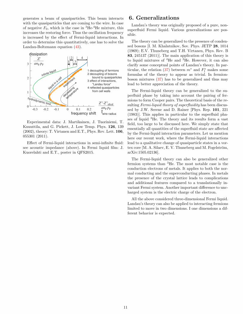
generates a beam of quasiparticles. This beam interactswith the quasiparticles that are coming to the wire. In caseof negative F0, which is the case in 3He-4He mixture, thisincreases the restoring force. Thus the oscillation frequencyis increased by the effect of Fermi-liquid interactions. Inorder to determine this quantitatively, one has to solve theLandau-Boltzmann equation (43).

Z'

anF pF

Z''-Z''ideal

anF pF-0.3 -0.2 -0.1 0 0.1 0.20

1

2

31

2

3

4

frequency shift

dissipation

1 decoupling of fermions

2 decoupling of bosons

bound to quasiparticles

3 effect of interactions,

"Landau force"

4 reflected quasiparticles

from cell wallsliq

uid

in a

cel

l

experim

ent

decr

easing

tem

pera

ture

infinte liquid

wire radius

hydrodynamic limit

Experimental data: J. Martikainen, J. Tuoriniemi, T.Knuuttila, and G. Pickett, J. Low Temp. Phys. 126, 139(2002), theory: T. Virtanen and E.T., Phys. Rev. Lett. 106,055301 (2011).

Effect of Fermi-liquid interactions in semi-infinite fluid:see acoustic impedance (above). In Fermi liquid film: J.Kuorelahti and E.T., poster in QFS2015.

6. GeneralizationsLandau’s theory was originally proposed of a pure, non-

superfluid Fermi liquid. Various generalizations are pos-sible.

The theory can be generalized to the presence of conden-sed bosons [I. M. Khalatnikov, Sov. Phys. JETP 28, 1014(1969); E.V. Thuneberg and T.H. Virtanen, Phys. Rev. B83, 245137 (2011)]. The main application of this theory isto liquid mixtures of 4He and 3He. However, it can alsoclarify some conceptual points of Landau’s theory. In par-ticular, the relation (37) between m∗ and F s1 makes someformulas of the theory to appear as trivial. In fermion-boson mixtures (37) has to be generalized and thus maylead to better appreciation of the theory.

The Fermi-liquid theory can be generalized to the su-perfluid phase by taking into account the pairing of fer-mions to form Cooper pairs. The theoretical basis of the re-sulting Fermi-liquid theory of superfluidity has been discus-sed by J.W. Serene and D. Rainer [Phys. Rep. 101, 221(1983)]. This applies in particular to the superfluid pha-ses of liquid 3He. The theory and its results form a vastfield, too large to be discussed here. We simply state thatessentially all quantities of the superfluid state are affectedby the Fermi-liquid interaction parameters. Let us mentionhere our recent work, where the Fermi-liquid interactionslead to a qualitative change of quasiparticle states in a vor-tex core [M. A. Silaev, E. V. Thuneberg and M. Fogelstrom,arXiv:1505.02136].

The Fermi-liquid theory can also be generalized otherfermion systems than 3He. The most notable case is theconduction electrons of metals. It applies to both the nor-mal conducting and the superconducting phases. In metalsthe presence of the crystal lattice leads to complicationsand additional features compared to a translationally in-variant Fermi system. Another important difference to unc-harged system is the electric charge of the electron.

All the above considered three-dimensional Fermi liquid.Landau’s theory can also be applied to interacting fermionslimited to move in two dimensions. I one dimensions a dif-ferent behavior is expected.

11

7. Derivation and limitationsLandau developed the Fermi-liquid theory intuitively as

the low energy expansion of a Fermi system. What it meansthat the Fermi-liquid state will appear if nothing else hap-pens. The possible alternative is that if the interactions arestrong enough, the particles will be localized and the sys-tem becomes solid instead of a liquid state. An interestingapproach to this is presented by R. Shankar [Rev. Mod.Phys. 66, 129 (1994)]. He uses the renormalization-groupmethod and finds that zooming into the neighborhood ofthe Fermi surface, the Fermi-liquid model appears as onealternative possibility.

The Fermi-liquid theory should appear as the low energylimit of a microscopic many-body theory. This means thatone should be able to calculate the Fermi-liquid parame-ters starting from a microscopic theory. At the moment itseems that the quantum-fluids community is using experi-mental values of the parameters. My hope is that some daythe many-body community would calculate more accuratevalues of the parameters.

8. ConclusionIn this introduction to the Landau’s Fermi-liquid theory

we have concentrated on its starting point. Especially wehave tried to clarify the nature of the quasiparticle. Outof the many applications of the theory to 3He and elsew-here we have only briefly mentioned a few. We hope thatunderstanding the elements of the theory gives good star-ting point to study the known applications, or finding newones.

12

Appendix: hydrodynamic model of a quasipar-ticle

The starting point is Euler’s equation and the equationof continuity

∂v

∂t+ v ·∇v = −1

ρ∇p

∂ρ

∂t+ ∇ · (ρv) = 0, (64)

where p is now the pressure. We assume a small veloci-ty so that the nonlinear term can be dropped and assumeincompressible fluid, ρ = constant. The boundary condi-tion on the surface of a sphere of radius a is n · v = n · u,where u is the velocity of the sphere and n the surfacenormal. We assume that far from the sphere v → 0. Thevelocity can be represented using the potential v = ∇χwhere χ = −a3u · r/2r3. By the Euler equation the pres-sure p = −ρχ, and the force exerted by the sphere on thefluid

F =

∫da p =

2πa3ρ

3u (65)

is proportional to the acceleration u. Therefore, associatedwith a moving sphere, there is momentum in the fluid

p =2πa3ρ

3u (66)

corresponding to half of the fluid displaced by the sphereand moving in the same direction and at the same velocityas the sphere. Note that this may differ from the totalmomentum of the fluid, which is not essential here, and isundetermined in the present limit of unlimited fluid.

13