AUTOMATION SYSTEM OPAC TUTORIAL Submitted by Shontel Howell, Ann Wilkinson,

8/6/2019 Tutorial ANN
http://slidepdf.com/reader/full/tutorial-ann 1/92
Tutorial on Neural
Networks
Prévotet Jean-Christophe
University of Paris VI
FRANCE

8/6/2019 Tutorial ANN
http://slidepdf.com/reader/full/tutorial-ann 2/92
Biological inspirations
Some numbers« The human brain contains about 10 billion nerve cells
(neurons)
Each neuron is connected to the others through10000 synapses
Properties of the brain
It can learn, reorganize itself from experience It adapts to the environment
It is robust and fault tolerant
8/6/2019 Tutorial ANN
http://slidepdf.com/reader/full/tutorial-ann 3/92
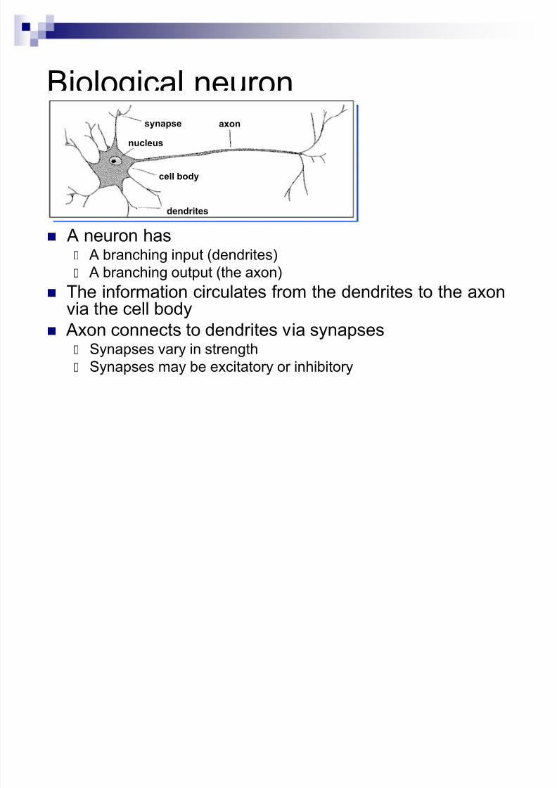
Biological neuron
A neuron has A branching input (dendrites)
A branching output (the axon)
The information circulates from the dendrites to the axonvia the cell body
Axon connects to dendrites via synapses Synapses vary in strength
Synapses may be excitatory or inhibitory
axon
cell body
synapse
nucleus
dendrites

8/6/2019 Tutorial ANN
http://slidepdf.com/reader/full/tutorial-ann 4/92
What is an artificial neuron ?
Definition : Non linear, parameterized function
with restricted output range
¹ º
¸©ª
¨! §
!
1
1
0
n
i
ii xww f y
x1 x2 x3
w0
y

8/6/2019 Tutorial ANN
http://slidepdf.com/reader/full/tutorial-ann 5/92
Activation functions
0 2 4 6 8 10 1 2 14 1 6 18 2 0 0
2
4
6
8
10
12
14
16
18
20
-10 - 8 -6 -4 -2 0 2 4 6 8 1 0 -2
-1.5
-1
-0.5
0
0.5
1
1.5
2
-10 - 8 -6 -4 -2 0 2 4 6 8 10
-2
-1.5
-1
-0.5
0
0.5
1
1.5
2
Linear
Logistic
Hyperbolic tangent
x y !
)exp(1
1
x y
!
)exp()exp(
)exp()exp(
x x
x x y
!
8/6/2019 Tutorial ANN
http://slidepdf.com/reader/full/tutorial-ann 6/92
Neural Networks A mathematical model to solve engineering problems
Group of highly connected neurons to realize compositions of non linear functions
Tasks Classification
Discrimination
Estimation
2 types of networks Feed forward Neural Networks
Recurrent Neural Networks

8/6/2019 Tutorial ANN
http://slidepdf.com/reader/full/tutorial-ann 7/92
Feed Forward Neural Networks The information is
propagated from theinputs to the outputs
Computations of No nonlinear functions from ninput variables bycompositions of Ncalgebraic functions
Time has no role (NOcycle between outputsand inputs)
x1 x2 xn«..
1st hidden
layer
2nd hidden
layer
Output layer

8/6/2019 Tutorial ANN
http://slidepdf.com/reader/full/tutorial-ann 8/92
Recurrent Neural Networks Can have arbitrary topologies
Can model systems withinternal states (dynamic ones)
Delays are associated to aspecific weight
Training is more difficult
Performance may beproblematic
Stable Outputs may be moredifficult to evaluate
Unexpected behavior (oscillation, chaos, «)
x1 x2
1
010
10
00

8/6/2019 Tutorial ANN
http://slidepdf.com/reader/full/tutorial-ann 9/92
Learning The procedure that consists in estimating the parameters of neurons
so that the whole network can perform a specific task
2 types of learning The supervised learning
The unsupervised learning
The Learning process (supervised) Present the network a number of inputs and their corresponding outputs
See how closely the actual outputs match the desired ones Modify the parameters to better approximate the desired outputs

8/6/2019 Tutorial ANN
http://slidepdf.com/reader/full/tutorial-ann 10/92
Supervised learning The desired response of the neural
network in function of particular inputs is
well known.
A ³Professor´ may provide examples and
teach the neural network how to fulfill a
certain task
8/6/2019 Tutorial ANN
http://slidepdf.com/reader/full/tutorial-ann 11/92
Unsupervised learning Idea : group typical input data in function of
resemblance criteria un-known a priori
Data clustering No need of a professor
The network finds itself the correlations between thedata
Examples of such networks : Kohonen feature maps

8/6/2019 Tutorial ANN
http://slidepdf.com/reader/full/tutorial-ann 12/92
Properties of Neural Networks Supervised networks are universal approximators (Non
recurrent networks)
Theorem : Any limited function can be approximated bya neural network with a finite number of hidden neuronsto an arbitrary precision
Type of Approximators Linear approximators : for a given precision, the number of
parameters grows exponentially with the number of variables(polynomials)
Non-linear approximators (NN), the number of parameters growslinearly with the number of variables

8/6/2019 Tutorial ANN
http://slidepdf.com/reader/full/tutorial-ann 13/92
Other properties Adaptivity
Adapt weights to environment and retrained easily
Generalization ability May provide against lack of data
Fault tolerance
Graceful degradation of performances if damaged =>
The information is distributed within the entire net.

8/6/2019 Tutorial ANN
http://slidepdf.com/reader/full/tutorial-ann 14/92
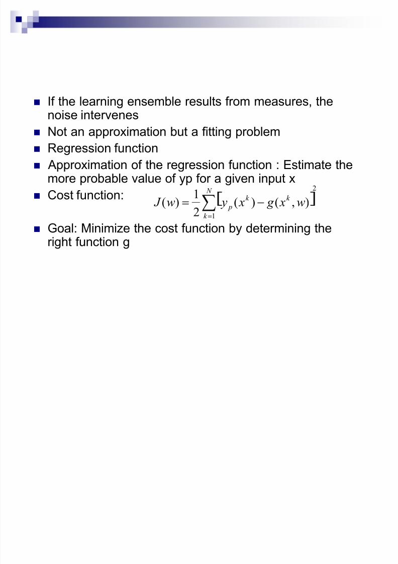
In practice, it is rare to approximate a known
function by a uniform function
³black box´ modeling : model of a process
The y output variable depends on the input
variable x with k=1 to N
Goal : Express this dependency by a function,for example a neural network
Static modeling
_ ak
p
k y x ,
8/6/2019 Tutorial ANN
http://slidepdf.com/reader/full/tutorial-ann 15/92

8/6/2019 Tutorial ANN
http://slidepdf.com/reader/full/tutorial-ann 16/92
Example

8/6/2019 Tutorial ANN
http://slidepdf.com/reader/full/tutorial-ann 17/92
Classification (Discrimination) Class objects in defined categories
Rough decision OR
Estimation of the probability for a certain
object to belong to a specific class
Example : Data mining
Applications : Economy, speech and
patterns recognition, sociology, etc.

8/6/2019 Tutorial ANN
http://slidepdf.com/reader/full/tutorial-ann 18/92
Example
Examples of handwritten postal codes
drawn from a database available from the US Postal service

8/6/2019 Tutorial ANN
http://slidepdf.com/reader/full/tutorial-ann 19/92
What do we need to use NN ?
Determination of pertinent inputs
Collection of data for the learning and testing
phase of the neural network Finding the optimum number of hidden nodes
Estimate the parameters (Learning)
Evaluate the performances of the network
IF performances are not satisfactory then reviewall the precedent points

8/6/2019 Tutorial ANN
http://slidepdf.com/reader/full/tutorial-ann 20/92
Classical neural architectures Perceptron
Multi-Layer Perceptron
Radial Basis Function (RBF)
Kohonen Features maps
Other architectures An example : Shared weights neural networks
8/6/2019 Tutorial ANN
http://slidepdf.com/reader/full/tutorial-ann 21/92
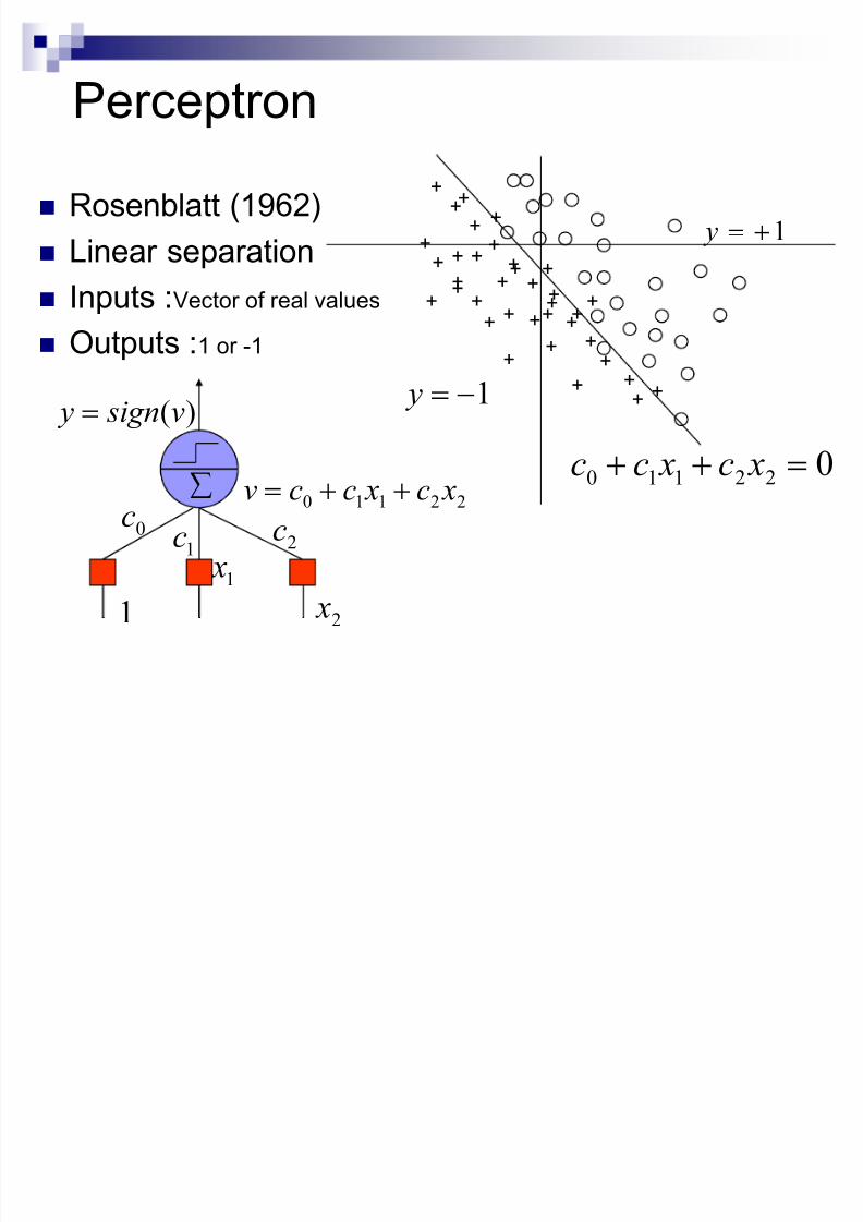
Perceptron
Rosenblatt (1962)
Linear separation
Inputs :Vector of real values
Outputs :1 or -1
022110 ! xc xcc
++
+
+
+
+
+
+
++
+ +
+
+ +
+
+
+++
+
+
++
+
+
+ ++
+
++
+
+
+
+
1! y
1! y
0c
1c 2
c
§
1 x
2 x1
22110xc xccv !
)(v sign y !
8/6/2019 Tutorial ANN
http://slidepdf.com/reader/full/tutorial-ann 22/92
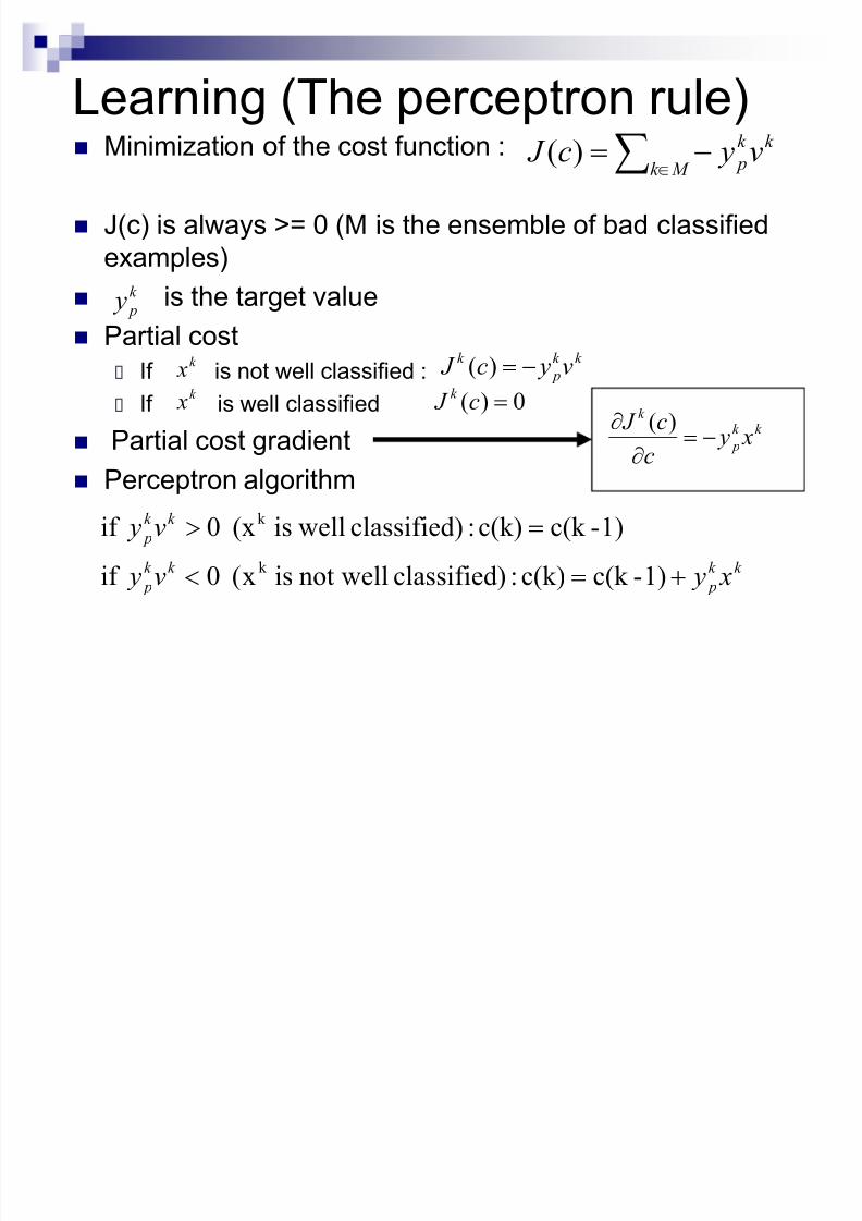
Learning (The perceptron rule) Minimization of the cost function :
J(c) is always >= 0 (M is the ensemble of bad classified
examples)
is the target value Partial cost
If is not well classified :
If is well classified
Partial cost gradient Perceptron algorithm
k x
§ � ! M k
k k
pv yc J )(
k
p y
k k
p
k k
p
k k
p
x yv y
v y
!
!"
1)-c(k c(k):)classifiednot wellisx( 0if
1)-c(k c(k):)classifiedwellis(x 0if
k
k
k x
k k
p
k v yc J !)(
0)( !c J k
k k
p
k
x yc
c J !
x
x )(

8/6/2019 Tutorial ANN
http://slidepdf.com/reader/full/tutorial-ann 23/92
The perceptron algorithm converges if
examples are linearly separable

8/6/2019 Tutorial ANN
http://slidepdf.com/reader/full/tutorial-ann 24/92
Multi-Layer Perceptron One or more hidden
layers
Sigmoid activationsfunctions
1st hidden
layer
2nd hidden
layer
Output layer
Input data

8/6/2019 Tutorial ANN
http://slidepdf.com/reader/full/tutorial-ann 25/92
8/6/2019 Tutorial ANN
http://slidepdf.com/reader/full/tutorial-ann 26/92
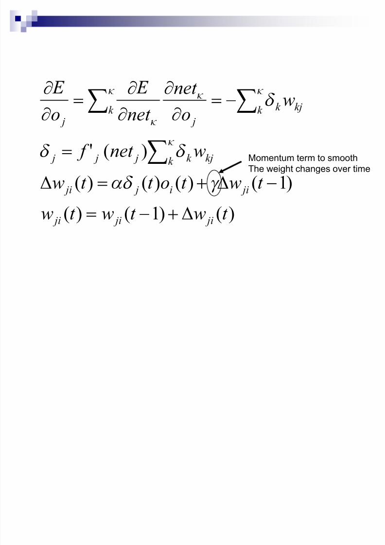
)()1()(
)1()()()(
)(
t wt wt w
t wt ot t w
wnet f
wo
net
net o
ji ji ji
jii j ji
k k jk j j j
k k k jk
j j
(!
(!(
!
!x
x
x
x!
x
x
§
§ §
K EH
H H
H
O
O O O
O
Momentum term to smooth
The weight changes over time

8/6/2019 Tutorial ANN
http://slidepdf.com/reader/full/tutorial-ann 27/92
S tructureTy pes of
Decision Regions
xclusive-OR
Problem
Classes with
eshed regions
ost General
Region S ha pes
S ingle-Layer
T wo-Layer
Three-Layer
Half Plane
Bounded By Hy per plane
Convex O pen
Or
Closed Regions
Abitrary
(Complexity
Limited by No.
o Nodes)
A
AB
B
A
AB
B
A
AB
B
BA
BA
BA
Different non linearly separable
problems
Neural Networks ± An Introduction Dr. Andrew Hunter

8/6/2019 Tutorial ANN
http://slidepdf.com/reader/full/tutorial-ann 28/92
RadialB
asis Functions (RB
Fs) Features
One hidden layer The activation of a hidden unit is determined by the distance between
the input vector and a prototype vector
Radial units
Outputs
Inputs

8/6/2019 Tutorial ANN
http://slidepdf.com/reader/full/tutorial-ann 29/92
RBF hidden layer units have a receptivefield which has a centre
Generally, the hidden unit function is
Gaussian
The output Layer is linear
Realized function
§
!*!
K
jj j c xW x s
1)(
2
exp¹¹¹
º
¸
©©©
ª
¨ !*
j
j
j
c xc x
W

8/6/2019 Tutorial ANN
http://slidepdf.com/reader/full/tutorial-ann 30/92
Learning
The training is performed by deciding on
How many hidden nodes there should be
The centers and the sharpness of the Gaussians
2 steps
In the 1st stage, the input data set is used to
determine the parameters of the basis functions
In the 2nd stage, functions are kept fixed while thesecond layer weights are estimated ( Simple BP
algorithm like for MLPs)

8/6/2019 Tutorial ANN
http://slidepdf.com/reader/full/tutorial-ann 31/92
MLPs versus RBFs Classification
MLPs separate classes viahyperplanes
RBFs separate classes viahyperspheres
Learning MLPs use distributed learning
RBFs use localized learning
RBFs train faster
Structure
MLPs have one or morehidden layers
RBFs have only one layer
RBFs require more hiddenneurons => curse of dimensionality
X2
X1
MLP
X2
X1
RBF

8/6/2019 Tutorial ANN
http://slidepdf.com/reader/full/tutorial-ann 32/92
Self organizing maps
The purpose of SOM is to map a multidimensional inputspace onto a topology preserving map of neurons Preserve a topological so that neighboring neurons respond to
similar »input patterns The topological structure is often a 2 or 3 dimensional space
Each neuron is assigned a weight vector with the samedimensionality of the input space
Input patterns are compared to each weight vector and
the closest wins (Euclidean Distance)

8/6/2019 Tutorial ANN
http://slidepdf.com/reader/full/tutorial-ann 33/92
The activation of theneuron is spread in itsdirect neighborhood
=>neighbors becomesensitive to the sameinput patterns
Block distance
The size of theneighborhood is initiallylarge but reduce over time => Specialization of the network
First neighborhood
2nd neighborhood

8/6/2019 Tutorial ANN
http://slidepdf.com/reader/full/tutorial-ann 34/92
Adaptation
During training, the³winner´ neuron and itsneighborhood adapts to
make their weight vector more similar to the inputpattern that caused theactivation
The neurons are movedcloser to the input pattern
The magnitude of theadaptation is controlledvia a learning parameter which decays over time

8/6/2019 Tutorial ANN
http://slidepdf.com/reader/full/tutorial-ann 35/92
Shared weights neural networks:
Time Delay Neural Networks (TDNNs) Introduced by Waibel in 1989
Properties
Local, shift invariant feature extraction Notion of receptive fields combining local information
into more abstract patterns at a higher level
Weight sharing concept (All neurons in a featureshare the same weights) All neurons detect the same feature but in different position
Principal Applications Speech recognition
Image analysis
8/6/2019 Tutorial ANN
http://slidepdf.com/reader/full/tutorial-ann 36/92
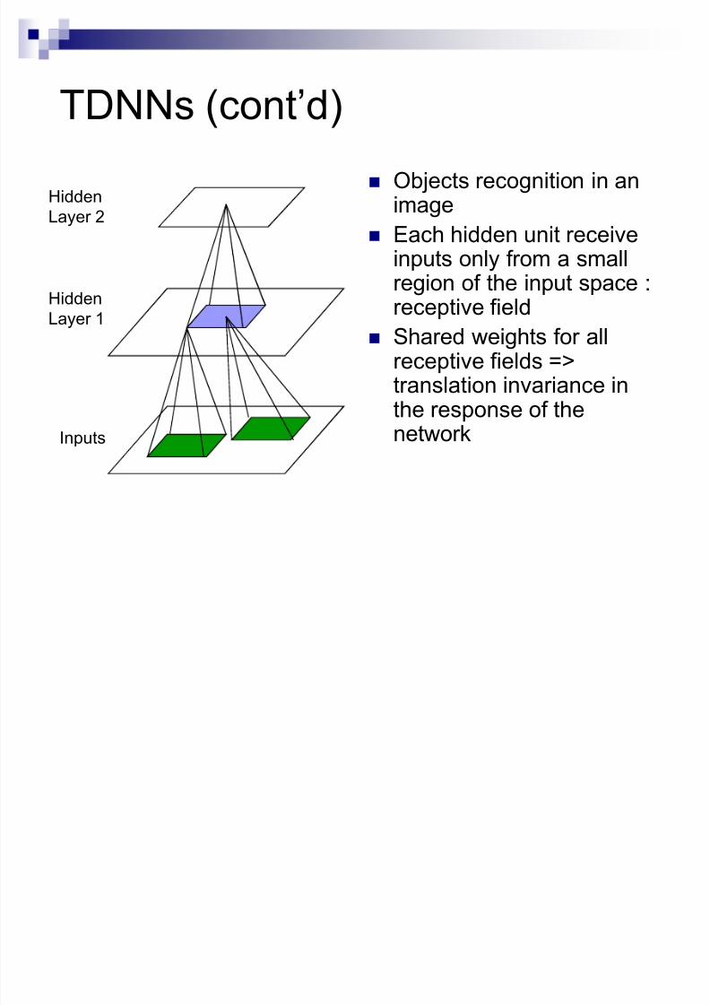
TDNNs (cont¶d)
Objects recognition in animage
Each hidden unit receive
inputs only from a smallregion of the input space :receptive field
Shared weights for allreceptive fields =>translation invariance inthe response of thenetworkInputs
Hidden
Layer 1
Hidden
Layer 2

8/6/2019 Tutorial ANN
http://slidepdf.com/reader/full/tutorial-ann 37/92
Advantages
Reduced number of weights
Require fewer examples in the training set
Faster learning
Invariance under time or space translation
Faster execution of the net (in comparison of full connected MLP)

8/6/2019 Tutorial ANN
http://slidepdf.com/reader/full/tutorial-ann 38/92
Neural Networks (Applications)
Face recognition
Time series prediction
Process identification
Process control
Optical character recognition
Adaptative filtering Etc«

8/6/2019 Tutorial ANN
http://slidepdf.com/reader/full/tutorial-ann 39/92
Conclusion on Neural Networks
Neural networks are utilized as statistical tools Adjust non linear functions to fulfill a task
Need of multiple and representative examples but fewer than in other methods
Neural networks enable to model complex static phenomena (FF) aswell as dynamic ones (RNN)
NN are good classifiers BUT Good representations of data have to be formulated
Training vectors must be statistically representative of the entire inputspace
Unsupervised techniques can help The use of NN needs a good comprehension of the problem

8/6/2019 Tutorial ANN
http://slidepdf.com/reader/full/tutorial-ann 40/92
Preprocessing
8/6/2019 Tutorial ANN
http://slidepdf.com/reader/full/tutorial-ann 41/92
Why Preprocessing ?
The curse of Dimensionality
The quantity of training data grows
exponentially with the dimension of the inputspace
In practice, we only have limited quantity of
input data
Increasing the dimensionality of the problem leads
to give a poor representation of the mapping
8/6/2019 Tutorial ANN
http://slidepdf.com/reader/full/tutorial-ann 42/92
Preprocessing methods
Normalization
Translate input values so that they can be
exploitable by the neural network
Component reduction
Build new input variables in order to reducetheir number
No Lost of information about their distribution

8/6/2019 Tutorial ANN
http://slidepdf.com/reader/full/tutorial-ann 43/92
Character recognition example
Image 256x256 pixels
8 bits pixels values
(grey level)
Necessary to extract
features
imagesdi erent1021580008256256
}vv

8/6/2019 Tutorial ANN
http://slidepdf.com/reader/full/tutorial-ann 44/92
Normalization
Inputs of the neural net are often of different types with different orders of
magnitude (E.g. Pressure, Temperature,etc.)
It is necessary to normalize the data sothat they have the same impact on the
model
Center and reduce the variables

8/6/2019 Tutorial ANN
http://slidepdf.com/reader/full/tutorial-ann 45/92
§ !!
N
n
n
ii x N
x1
1
§ !
!
N
n i
n
ii x x N
1
22
1
1W
i
i
n
in
i
x x
x W
!
Average on all points
Variance calculation
Variables transposition
8/6/2019 Tutorial ANN
http://slidepdf.com/reader/full/tutorial-ann 46/92
Components reduction
Sometimes, the number of inputs is too large to
be exploited
The reduction of the input number simplifies theconstruction of the model
Goal : Better representation of the data in order
to get a more synthetic view without losing
relevant information
Reduction methods (PCA, CCA, etc.)
8/6/2019 Tutorial ANN
http://slidepdf.com/reader/full/tutorial-ann 47/92
Principal Components Analysis
(PCA) Principle
Linear projection method to reduce the number of parameters
Transfer a set of correlated variables into a new set of
uncorrelated variables Map the data into a space of lower dimensionality
Form of unsupervised learning
Properties It can be viewed as a rotation of the existing axes to new
positions in the space defined by original variables New axes are orthogonal and represent the directions with
maximum variability
8/6/2019 Tutorial ANN
http://slidepdf.com/reader/full/tutorial-ann 48/92
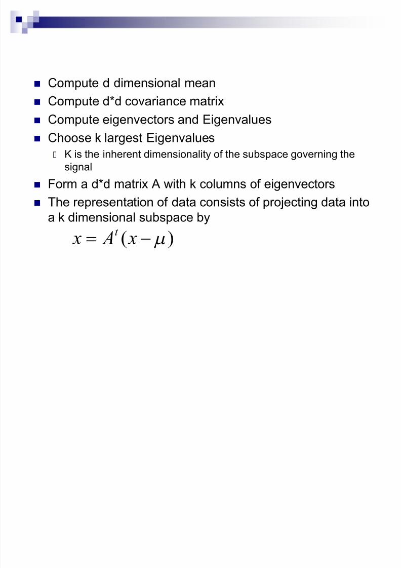
Compute d dimensional mean
Compute d*d covariance matrix
Compute eigenvectors and Eigenvalues
Choose k largest Eigenvalues K is the inherent dimensionality of the subspace governing the
signal
Form a d*d matrix A with k columns of eigenvectors
The representation of data consists of projecting data into
a k dimensional subspace by
)( Q! x A x t

8/6/2019 Tutorial ANN
http://slidepdf.com/reader/full/tutorial-ann 49/92
Example of data representation
using PCA

8/6/2019 Tutorial ANN
http://slidepdf.com/reader/full/tutorial-ann 50/92
Limitations of PCA
The reduction of dimensions for complex
distributions may need non linear
processing
8/6/2019 Tutorial ANN
http://slidepdf.com/reader/full/tutorial-ann 51/92
Curvilinear Components
Analysis Non linear extension of the PCA
Can be seen as a self organizing neural network
Preserves the proximity between the points inthe input space i.e. local topology of the
distribution
Enables to unfold some varieties in the input
data
Keep the local topology
8/6/2019 Tutorial ANN
http://slidepdf.com/reader/full/tutorial-ann 52/92
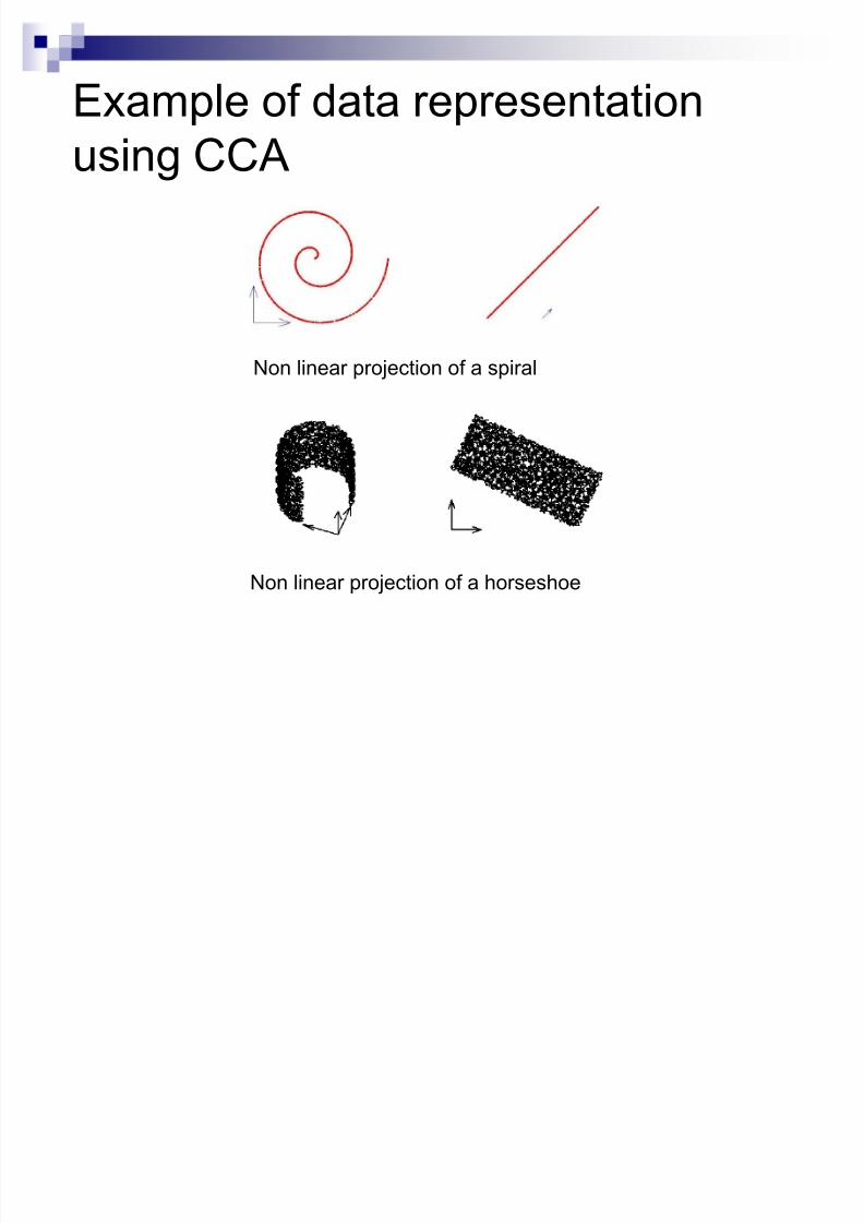
Example of data representation
using CCA
Non linear projection of a horseshoe
Non linear projection of a spiral
8/6/2019 Tutorial ANN
http://slidepdf.com/reader/full/tutorial-ann 53/92
Other methods
Neural pre-processing
Use a neural network to reduce the
dimensionality of the input space
Overcomes the limitation of PCA
Auto-associative mapping => form of
unsupervised training

8/6/2019 Tutorial ANN
http://slidepdf.com/reader/full/tutorial-ann 54/92
x1 x2 xd«.
x1 x2 xd«.
z1 zM
Transformation of a d
dimensional input space
into a M dimensional
output space
Non linear component
analysis
The dimensionality of the
sub-space must bedecided in advance
D dimensional input space
D dimensional output space
M dimensional sub-space
8/6/2019 Tutorial ANN
http://slidepdf.com/reader/full/tutorial-ann 55/92
« Intelligent preprocessing »
Use an ³a priori´ knowledge of the problem
to help the neural network in performing its
task
Reduce manually the dimension of the
problem by extracting the relevant features
More or less complex algorithms toprocess the input data
8/6/2019 Tutorial ANN
http://slidepdf.com/reader/full/tutorial-ann 56/92
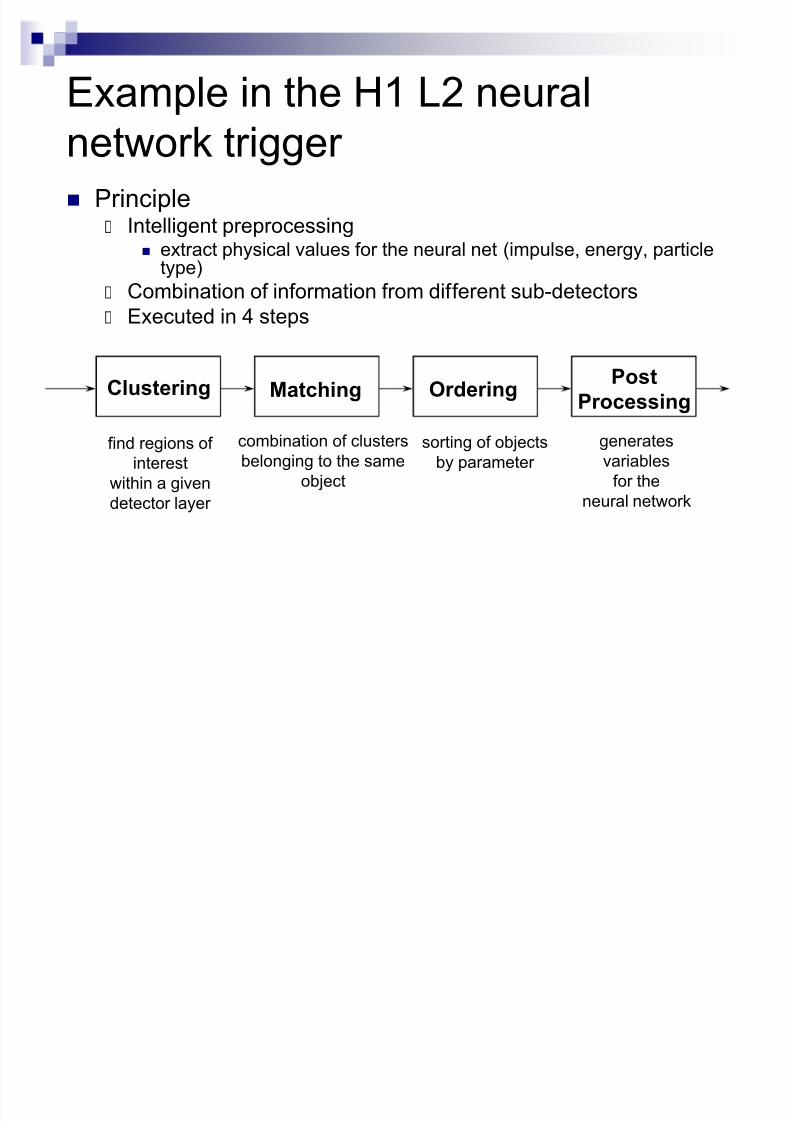
Example in the H1 L2 neural
network trigger Principle
Intelligent preprocessing extract physical values for the neural net (impulse, energy, particle
type)
Combination of information from different sub-detectors Executed in 4 steps
Clustering Matching OrderingPost
Processing
find regions of
interest
within a given
detector layer
combination of clusters
belonging to the same
object
sorting of objects
by parameter
generates
variables
for the
neural network

8/6/2019 Tutorial ANN
http://slidepdf.com/reader/full/tutorial-ann 57/92
Conclusion on the preprocessing
The preprocessing has a huge impact onperformances of neural networks
The distinction between the preprocessing and
the neural net is not always clear The goal of preprocessing is to reduce the
number of parameters to face the challenge of ³curse of dimensionality´
It exists a lot of preprocessing algorithms andmethods Preprocessing with prior knowledge
Preprocessing without

8/6/2019 Tutorial ANN
http://slidepdf.com/reader/full/tutorial-ann 58/92
Implementation of neural
networks

8/6/2019 Tutorial ANN
http://slidepdf.com/reader/full/tutorial-ann 59/92
Motivations and questions
Which architectures utilizing to implement Neural Networks in real-time ? What are the type and complexity of the network ?
What are the timing constraints (latency, clock frequency, etc.)
Do we need additional features (on-line learning, etc.)? Must the Neural network be implemented in a particular environment (
near sensors, embedded applications requiring less consumption etc.) ?
When do we need the circuit ?
Solutions Generic architectures
Specific Neuro-Hardware Dedicated circuits
8/6/2019 Tutorial ANN
http://slidepdf.com/reader/full/tutorial-ann 60/92
Generic hardware architectures
Conventional microprocessors
Intel Pentium, Power PC, etc «
Advantages High performances (clock frequency, etc)
Cheap
Software environment available (NN tools, etc)
Drawbacks Too generic, not optimized for very fast neural
computations
8/6/2019 Tutorial ANN
http://slidepdf.com/reader/full/tutorial-ann 61/92
Specific Neuro-hardware circuits
Commercial chips CNAPS, Synapse, etc.
Advantages Closer to the neural applications
High performances in terms of speed Drawbacks
Not optimized to specific applications
Availability
Development tools
Remark These commercials chips tend to be out of production

8/6/2019 Tutorial ANN
http://slidepdf.com/reader/full/tutorial-ann 62/92
Example :CNAPS Chip
64 x 64 x 1 in 8 µs
(8 bit inputs, 16 bit weight
CNAPS 1064 chip
Adaptive Solutions,
Oregon

8/6/2019 Tutorial ANN
http://slidepdf.com/reader/full/tutorial-ann 63/92

8/6/2019 Tutorial ANN
http://slidepdf.com/reader/full/tutorial-ann 64/92
Dedicated circuits
A system where the functionality is once and for
all tied up into the hard and soft-ware.
Advantages Optimized for a specific application
Higher performances than the other systems
Drawbacks
High development costs in terms of time and money
8/6/2019 Tutorial ANN
http://slidepdf.com/reader/full/tutorial-ann 65/92
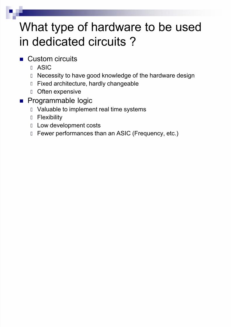
What type of hardware to be used
in dedicated circuits ? Custom circuits
ASIC
Necessity to have good knowledge of the hardware design
Fixed architecture, hardly changeable Often expensive
Programmable logic Valuable to implement real time systems
Flexibility
Low development costs Fewer performances than an ASIC (Frequency, etc.)

8/6/2019 Tutorial ANN
http://slidepdf.com/reader/full/tutorial-ann 66/92
Programmable logic
Field Programmable Gate Arrays (FPGAs)
Matrix of logic cells
Programmable interconnection
Additional features (internal memories +
embedded resources like multipliers, etc.)
Reconfigurability We can change the configurations as many times
as desired

8/6/2019 Tutorial ANN
http://slidepdf.com/reader/full/tutorial-ann 67/92
FPGA Architecture
I/O Ports
Block Rams
Programmableconnections
ProgrammableLogicBlocks
DLL
LUT
LUT
Carry &
Control
Carry &
Control
D Q
D Q
y
yq
x b
x
xq
cin
cout
G4
G3
G2
G1
F4
F3
F2
F1
bx
X ilinx Virtex slice
8/6/2019 Tutorial ANN
http://slidepdf.com/reader/full/tutorial-ann 68/92
Real time Systems
Real-Time SystemsExecution of applications with time constraints.
hard and soft real-time systems
digital fly-by-wire control system of an aircraft:No lateness is accepted Cost. The lives of people depend onthe correct working of the control system of the aircraft.
A soft real-time system can be a vending machine:
Accept lower performance for lateness, it is not catastrophicwhen deadlines are not met. It will take longer to handle oneclient with the vending machine.

8/6/2019 Tutorial ANN
http://slidepdf.com/reader/full/tutorial-ann 69/92
Typical real time processing
problems In instrumentation, diversity of real-time
problems with specific constraints
Problem : Which architecture is adequatefor implementation of neural networks ?
Is it worth spending time on it?

8/6/2019 Tutorial ANN
http://slidepdf.com/reader/full/tutorial-ann 70/92
Some problems and dedicated
architectures ms scale real time system
Architecture to measure raindrops size and
velocity Connectionist retina for image processing
µs scale real time system
Level 1 trigger in a HEP experiment

8/6/2019 Tutorial ANN
http://slidepdf.com/reader/full/tutorial-ann 71/92
Architecture to measure raindrops
size and velocity
2 focalized beams on 2
photodiodes
Diodes deliver a signalaccording to the received
energy
The height of the pulse
depends on the radius Tp depends on the speed
of the droplet
Problematic
Tp

8/6/2019 Tutorial ANN
http://slidepdf.com/reader/full/tutorial-ann 72/92
Input data
High level of noise
Significant variation of
The current baseline
Real dropletNoise
8/6/2019 Tutorial ANN
http://slidepdf.com/reader/full/tutorial-ann 73/92
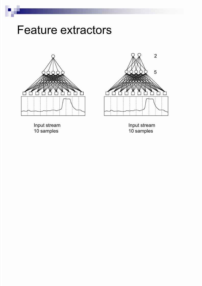
Feature extractors
5
2
Input stream
10 samples
Input stream
10 samples

8/6/2019 Tutorial ANN
http://slidepdf.com/reader/full/tutorial-ann 74/92
Proposed architecture
20 input indo s
Presence o a
droplet
Size
Full interconnectionFull interconnection
Velocity
Feature
extractors

8/6/2019 Tutorial ANN
http://slidepdf.com/reader/full/tutorial-ann 75/92
Performances
Estimated
Radii
(mm)
Actual Radii (mm)
EstimatedVelocities
(m/s)
Actual velocities (m/s)

8/6/2019 Tutorial ANN
http://slidepdf.com/reader/full/tutorial-ann 76/92
Hardware implementation
10 KHz Sampling
Previous times => neuro-hardware
accelerator (Totem chip from Neuricam)
Today, generic architectures are sufficient
to implement the neural network in real-
time

8/6/2019 Tutorial ANN
http://slidepdf.com/reader/full/tutorial-ann 77/92
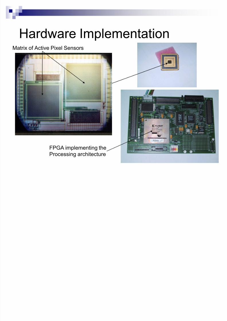
Connectionist Retina
Integration of a neuralnetwork in an artificialretina
Screen Matrix of Active Pixelsensors
CAN (8 bits converter)256 levels of grey
Processing Architecture Parallel system where
neural networks areimplemented
ProcessingArchitecture
CAN
I

8/6/2019 Tutorial ANN
http://slidepdf.com/reader/full/tutorial-ann 78/92
Processing architecture: ³The
maharaja´ chipIntegrated Neural Networks :
WEIGHTHED SUMWEIGHTHED SUM �i wiXi
EUCLIDEANEUCLIDEAN (A ± B)2
MANHATTANMANHATTAN |A ± B|
MAHALANOBISMAHALANOBIS (A ± B) � (A ± B)
Radial Basis function [RBF]
Multilayer Perceptron [MLP]
8/6/2019 Tutorial ANN
http://slidepdf.com/reader/full/tutorial-ann 79/92
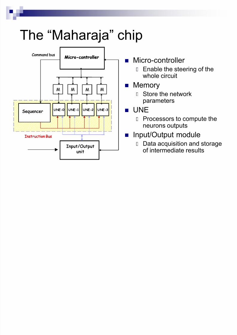
The ³Maharaja´ chip
Micro-controller Enable the steering of the
whole circuit
Memory Store the network
parameters
UNE Processors to compute the
neurons outputs Input/Output module
Data acquisition and storageof intermediate results
MicroMicro--controllercontroller
SequencerSequencer
Command busCommand bus
Input/OutputInput/Outputunitunit
Instruction BusInstruction Bus
UNE-0 UNE-1 UNE-2 UNE-3
M M M M
8/6/2019 Tutorial ANN
http://slidepdf.com/reader/full/tutorial-ann 80/92
Hardware Implementation
FPGA implementing the
Processing architecture
Matrix of Active Pixel Sensors

8/6/2019 Tutorial ANN
http://slidepdf.com/reader/full/tutorial-ann 81/92
Performances
Neural Networks
Performances
Latency(Timing constraints)
Estimatedexecution time
MLP (High Energy Physics)
(4-8-8-4) 10 µs 6,5 µs
RBF (Image processing)(4-10-256) 40 ms
473 µs (Manhattan)23ms
(Mahalanobis)
8/6/2019 Tutorial ANN
http://slidepdf.com/reader/full/tutorial-ann 82/92
Level 1 trigger in a HEP experiment
Neural networks have provided interestingresults as triggers in HEP.
Level 2 : H1 experiment Level 1 : Dirac experiment
Goal : Transpose the complex processingtasks of Level 2 into Level 1
High timing constraints (in terms of latencyand data throughput)
8/6/2019 Tutorial ANN
http://slidepdf.com/reader/full/tutorial-ann 83/92
««..
««..
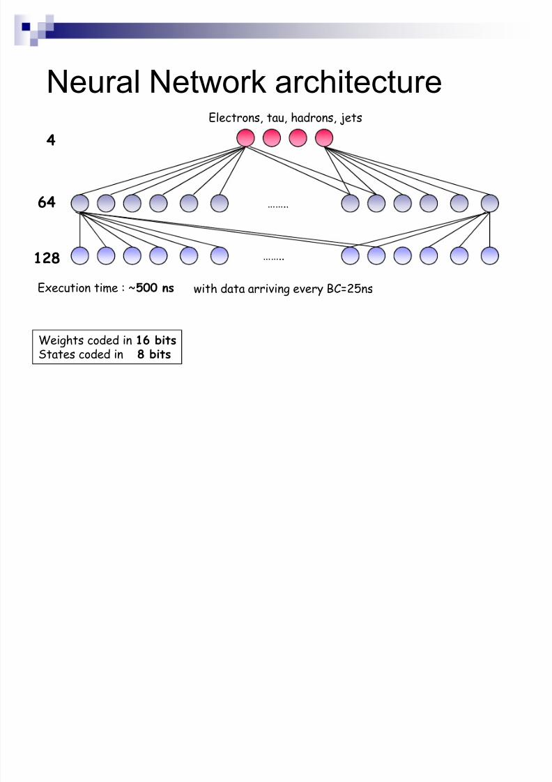
64
128
4
Execution time : ~500 ns
Weights coded in 16 bitsStates coded in 8 bits
with data arriving every BC=25ns
Electrons, tau, hadrons, jets
Neural Network architecture

8/6/2019 Tutorial ANN
http://slidepdf.com/reader/full/tutorial-ann 84/92
Very fast architecture Matrix of n*m matrix
elements
Control unit
I/O module
TanH are stored in
LUTs 1 matrix row
computes a neuron
The results is back-propagated tocalculate the output
layer
TanH
PE
256 PEs for a 128x64x4 network
PE PEPE
PE PE PEPE
PE PE PEPE
PE PE PEPE
TanH
TanH
TanH
ACC
ACC
ACC
ACC
I/O module
Control unit
8/6/2019 Tutorial ANN
http://slidepdf.com/reader/full/tutorial-ann 85/92
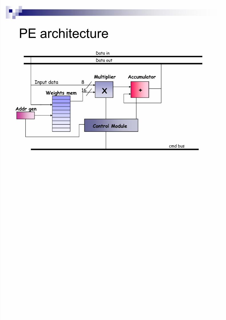
PE architecture
X
AccumulatorMultiplier
Weights mem
Input data 816
Addr gen
+
Data in
cmd bus
Control Module
Data out

8/6/2019 Tutorial ANN
http://slidepdf.com/reader/full/tutorial-ann 86/92
Technological Features
4 input buses (data are coded in 8 bits)
1 output bus (8 bits)
Processing Elements
Signed multipliers 16x8 bits
Accumulation (29 bits)
Weight memories (64x16 bits)
Look Up Tables
Addresses in 8 bitsData in 8 bits
Internal speed
Inputs/Outputs
T argeted to be 120 MHz
8/6/2019 Tutorial ANN
http://slidepdf.com/reader/full/tutorial-ann 87/92
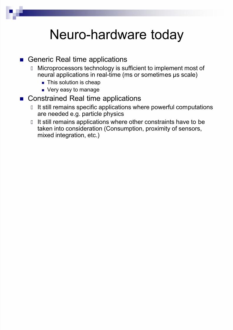
Neuro-hardware today
Generic Real time applications Microprocessors technology is sufficient to implement most of
neural applications in real-time (ms or sometimes µs scale)
This solution is cheap
Very easy to manage
Constrained Real time applications It still remains specific applications where powerful computations
are needed e.g. particle physics
It still remains applications where other constraints have to betaken into consideration (Consumption, proximity of sensors,mixed integration, etc.)
8/6/2019 Tutorial ANN
http://slidepdf.com/reader/full/tutorial-ann 88/92
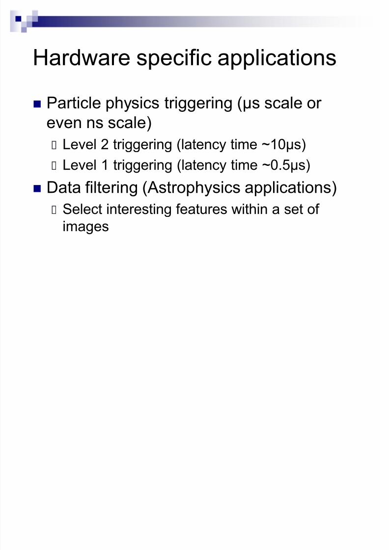
Hardware specific applications
Particle physics triggering (µs scale or
even ns scale)
Level 2 triggering (latency time ~10µs) Level 1 triggering (latency time ~0.5µs)
Data filtering (Astrophysics applications)
Select interesting features within a set of images

8/6/2019 Tutorial ANN
http://slidepdf.com/reader/full/tutorial-ann 89/92
For generic applications : trend of
clustering Idea : Combine performances of different
processors to perform massive parallel
computations
High speed
connection
8/6/2019 Tutorial ANN
http://slidepdf.com/reader/full/tutorial-ann 90/92
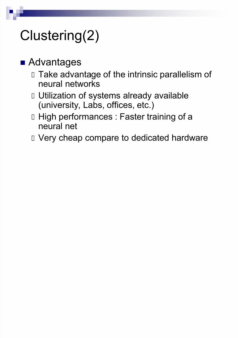
Clustering(2)
Advantages
Take advantage of the intrinsic parallelism of
neural networks Utilization of systems already available
(university, Labs, offices, etc.)
High performances : Faster training of a
neural net Very cheap compare to dedicated hardware

8/6/2019 Tutorial ANN
http://slidepdf.com/reader/full/tutorial-ann 91/92
Clustering(3)
Drawbacks
Communications load : Need of very fast links
between computers Software environment for parallel processing
Not possible for embedded applications

8/6/2019 Tutorial ANN
http://slidepdf.com/reader/full/tutorial-ann 92/92
Conclusion on the Hardware
Implementation Most real-time applications do not need dedicated
hardware implementation Conventional architectures are generally appropriate
Clustering of generic architectures to combine performances Some specific applications require other solutions
Strong Timing constraints
Technology permits to utilize FPGAs
Flexibility
Massive parallelism possible
Other constraints (consumption, etc.)
Custom or programmable circuits