Turbulent boundary layer separation andcontrol

by

Ola Logdberg

December 2008Technical Reports from

Royal Institute of TechnologyKTH Mechanics

SE-100 44 Stockholm, Sweden

Akademisk avhandling som med tillstand av Kungliga Tekniska Hogskolan iStockholm framlagges till offentlig granskning for avlaggande av teknologiedoktorsexamen fredagen den 23 januari 2009 kl 10.15 i F3, Kungliga TekniskaHogskolan, Lindstedtsvagen 26, Stockholm.

c©Ola Logdberg 2008

Universitetsservice US–AB, Stockholm 2008

Ola Logdberg 2008, Turbulent boundary layer separation and controlLinne Flow Centre, KTH Mechanics, SE-100 44 Stockholm, Sweden

AbstractBoundary layer separation is an unwanted phenomenon in most technical ap-plications, as for instance on airplane wings, ground vehicles and in internalflow systems. If separation occurs, it causes loss of lift, higher drag and energylosses. It is thus essential to develop methods to eliminate or delay separation.

In the present experimental work streamwise vortices are introduced in tur-bulent boundary layers to transport higher momentum fluid towards the wall.This enables the boundary layer to stay attached at larger pressure gradients.First the adverse pressure gradient (APG) separation bubbles that are to beeliminated are studied. It is shown that, independent of pressure gradient,the mean velocity defect profiles are self-similar when the scaling proposed byZagarola and Smits is applied to the data. Then vortex pairs and arrays of vor-tices of different initial strength are studied in zero pressure gradient (ZPG).Vane-type vortex generators (VGs) are used to generate counter-rotating vor-tex pairs, and it is shown that the vortex core trajectories scale with the VGheight h and the spanwise spacing of the blades. Also the streamwise evolu-tion of the turbulent quantities scale with h. As the vortices are convecteddownstream they seem to move towards a equidistant state, where the distancefrom the vortex centres to the wall is half the spanwise distance between twovortices. Yawing the VGs up to 20 do not change the generated circulation ofa VG pair. After the ZPG measurements, the VGs where applied in the APGmentioned above. It is shown that that the circulation needed to eliminateseparation is nearly independent of the pressure gradient and that the stream-wise position of the VG array relative to the separated region is not critical tothe control effect. In a similar APG jet vortex generators (VGJs) are shown toas effective as the passive VGs. The ratio VR of jet velocity and test sectioninlet velocity is varied and a control effectiveness optimum is found for VR = 5.At 40 yaw the VGJs have only lost approximately 20 % of the control effect.For pulsed VGJs the pulsing frequency, the duty cycle and VR were varied. Itwas shown that to achieve maximum control effect the injected mass flow rateshould be as large as possible, within an optimal range of jet VRs. For a giveninjected mass flow rate, the important parameter was shown to be the injectiontime t1. A non-dimensional injection time is defined as t+1 = t1Ujet/d, where dis the jet orifice diameter. Here, the optimal t+1 was 100–200.Descriptors: Flow control, adverse pressure gradient (APG), flow separa-tion, vortex generators, jet vortex generators, pulsed jet vortex generators.

iii

Preface

This doctoral thesis in fluid mechanics is a paper-based thesis of experimentalcharacter. The subject of the thesis is turbulent boundary layer separationcontrol by means of longitudinal vortices. The thesis is divided into two partsin where the first part is an overview and summary of the present contributionto the field of fluid mechanics. The second part consists of five papers, which areadjusted to comply with the present thesis format for consistency. In chapter 7of the first part in the thesis the respondent’s contribution to all papers arestated.

December 2008, StockholmOla Logdberg

iv

Contents

Abstract iii

Preface iv

Part I. Overview and summary

Chapter 1. Introduction 11.1. Truck aerodynamics 21.2. Research outline 6

Chapter 2. Separation 72.1. The separated region 72.2. The Zagarola-Smits velocity scale 9

Chapter 3. Vane-type vortex generators 133.1. Vane-type VGs in ZPG 133.2. Vane-type VGs in APG 19

Chapter 4. Jet vortex generators 234.1. Steady jet VGs 234.2. Pulsed jet VGs 27

Chapter 5. Conclusions 315.1. The separated region 315.2. Vane-type VGs 315.3. Jet VGs 32

Chapter 6. Outlook 336.1. Practical applications 336.2. Further research 33

Chapter 7. Papers and authors contributions 35

v

Acknowledgements 38

References 39

Part II. Papers

1. On the scaling of turbulent separating boundary layers 47

2. Streamwise evolution of longitudinal vortices in aturbulent boundary layer 61

3. On the robustness of separation control by streamwisevortices 105

4. Separation control by an array of vortex generator jets.Part 1. Steady jets. 129

5. Separation control by an array of vortex generator jets.Part 2. Pulsed jets. 159

vi

Part I

Overview and summary

CHAPTER 1

Introduction

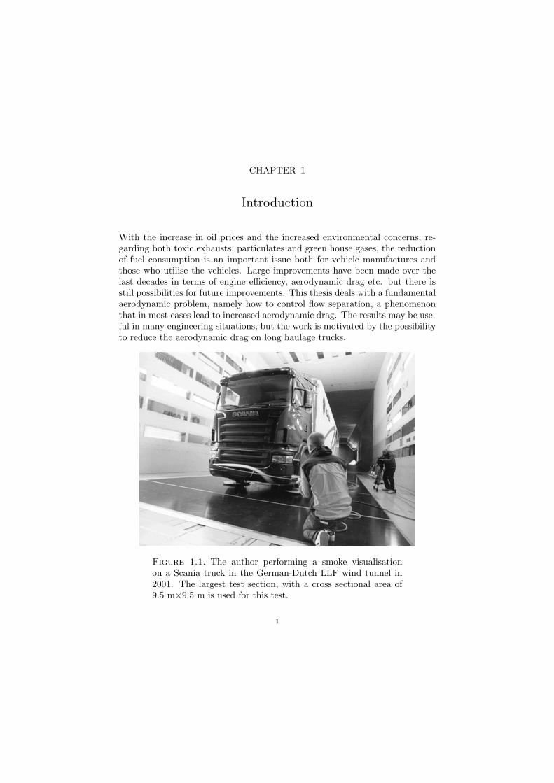
With the increase in oil prices and the increased environmental concerns, re-garding both toxic exhausts, particulates and green house gases, the reductionof fuel consumption is an important issue both for vehicle manufactures andthose who utilise the vehicles. Large improvements have been made over thelast decades in terms of engine efficiency, aerodynamic drag etc. but there isstill possibilities for future improvements. This thesis deals with a fundamentalaerodynamic problem, namely how to control flow separation, a phenomenonthat in most cases lead to increased aerodynamic drag. The results may be use-ful in many engineering situations, but the work is motivated by the possibilityto reduce the aerodynamic drag on long haulage trucks.

Figure 1.1. The author performing a smoke visualisationon a Scania truck in the German-Dutch LLF wind tunnel in2001. The largest test section, with a cross sectional area of9.5 m×9.5 m is used for this test.

1

2 1. INTRODUCTION

0 40 80 1200

100

200

300

400

500

U [km/h]

P [k

W]

P

P

aero

tire

Figure 1.2. The engine power needed to overcome aerody-namic drag Paero and tire rolling resistance Ptire. To producethis approximate plot the coefficients of wind averaged dragand rolling resistance were asumed to be CD,wa = 0.6 and fr= 0.0045.

1.1. Truck aerodynamics

The aerodynamic drag is an important part of the total average tractive re-sistance of a long-haulage truck. A heavy truck (for example the Scania R-series truck shown in figure 1.1), with warm low resistance tires, at a speedUx = 80 km/h on a flat dry road has a rolling resistance which is approximately50 % of the total tractive resistance. The remaining 50 % is aerodynamic drag.The rolling resistance coefficient fr is known to be almost independent of thespeed and therefore the drag caused by the tires increases linearly with thespeed (Fx,tire = frUx). Also the aerodynamic drag coefficient (CD) is fairlyindependent of the speed for a truck, which means that the aerodynamic dragFx,aero = 1

2ρCDU2x , where ρ is the density of the fluid, increases quadratically

with the speed. At speeds above approximately 80 km/h the contribution ofthe aerodynamic drag to the total drag overshadows that of the tires, as canbe seen i figure 1.2.

The analysis above is however oversimplified, since very few long haulageroutes in the real world are completely flat. Furthermore, vehicles occasionallyhave to slow down or even stop. Therefore it is necessary to take into accountboth ”hill climbing” and acceleration. According to simulations performed bythe author the aerodynamic drag constitutes around 30 % of the total drag onmoderately hilly long haulage routes, like Stockholm-Helsingborg. This is for a

1.1. TRUCK AERODYNAMICS 3

22

26

30

34

0.00 0.10 0.20 0.30 0.40 0.50 0.60 0.70500000

600000

700000

800000

D cost = 125 kkr

Scania R-series

Scania Concept Vehicle

CD,wa

Fuel

con

sum

ptio

n [l/

100

km]

Year

ly fu

el c

ost [

kr]

Figure 1.3. Fuel consumption and fuel cost for a truck usedin long haulage operation. The fuel cost is based on an annualmileage of 200000 km and the price of diesel oil in December2008 (11.40 kr/l). This is a slight overestimation since all largetransport companies get discounts on fuel.

truck trailer combination with a relatively smooth-sided trailer, low resistancetires and a modern 420 hp engine.

Since truck manufacturers do not develop tires and cannot change thetopography (although there are systems to store brake energy), or do muchabout the traffic situation, aerodynamic drag is the component of the tractiveresistance that is possible to reduce. Apart from the obvious environmentalbenefits of bringing down the fuel consumption, the economical gains are sub-stantial. Figure 1.3 demonstrates the relation between aerodynamic drag, fuelconsumption and the annual cost of fuel for a long haulage operator. The truckin figure 1.4 was developed at Scania in 1999 as a technology demonstrator andone of the main features was its low CD,wa

1. In figure 1.3 this concept vehicleis chosen to represent the realistic limit for aerodynamic drag reduction. TheScania R-series in figure 1.1 is typical for an aerodynamically well-designedtruck of today and the span of CD,wa given is a conservative estimation of thevariation due to trailer choice.

1Since CD increases with yaw for a normal truck, a wind averaged drag coefficient CD,wa is

calculated by averaging weighted CD measurements at different yaw angles.

4 1. INTRODUCTION

Figure 1.4. A Scania low drag concept truck from 1998. Theshown configuration is without the accompanying trailer.

A truck is a bluff body and a major part of the drag stems from pressure,which means that friction is less important. In the beginning of time, truckswere shaped like bricks, producing massive separation all around the front.During the 70s and 80s the front of the trucks went from sharp cornered torounded and air deflectors were fitted to the roof and the sides to smooth thetransition from the cab to the body. This is illustrated as the change from (a)to (b) in figure 1.5. When the front radii are greater than 300 mm and theair deflector kit is properly designed, there are no major improvements to bemade on the front. However, there are still many areas to improve on the sides,around the wheels and on the underbody, but in order to drastically reduceaerodynamic drag the separation at the end also needs to be addressed.

Early truck Today's truck Low drag truck(a) (b) (c)

Figure 1.5. The aerodynamic development of trucks sincethe 1970s.

1.1. TRUCK AERODYNAMICS 5

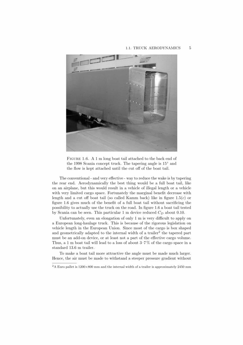
Figure 1.6. A 1 m long boat tail attached to the back end ofthe 1998 Scania concept truck. The tapering angle is 15 andthe flow is kept attached until the cut off of the boat tail.

The conventional - and very effective - way to reduce the wake is by taperingthe rear end. Aerodynamically the best thing would be a full boat tail, likeon an airplane, but this would result in a vehicle of illegal length or a vehiclewith very limited cargo space. Fortunately the marginal benefit decrease withlength and a cut off boat tail (so called Kamm back) like in figure 1.5(c) orfigure 1.6 gives much of the benefit of a full boat tail without sacrificing thepossibility to actually use the truck on the road. In figure 1.6 a boat tail testedby Scania can be seen. This particular 1 m device reduced CD about 0.10.

Unfortunately, even an elongation of only 1 m is very difficult to apply ona European long-haulage truck. This is because of the rigorous legislation onvehicle length in the European Union. Since most of the cargo is box shapedand geometrically adapted to the internal width of a trailer2 the tapered partmust be an add-on device, or at least not a part of the effective cargo volume.Thus, a 1 m boat tail will lead to a loss of about 3–7 % of the cargo space in astandard 13.6 m trailer.

To make a boat tail more attractive the angle must be made much larger.Hence, the air must be made to withstand a steeper pressure gradient without

2A Euro pallet is 1200×800 mm and the internal width of a trailer is approximately 2450 mm

6 1. INTRODUCTION

separation. In 2001 the author performed a wind tunnel test on a boat tail,where the boundary layer was energised using slot blowing. The device wasmounted on the 1:2 scale model shown in figure 1.4. With the blowing turned onthe maximum non-separating tapering angle increased from 15 to 25. Eventhough the concept was implemented in a very crude way the principle wasshown to work. However, the energy consumption of the fans needed to supplyair for the blowing slot was so high that it neutralised the gains from the dragreduction. Furthermore, the fans, valves and tubing needed not only reducesthe cargo volume but impede access. Therefore, it would be desirable to findanother technical solution for the separation control; one that would have asimilar effect but would be easier to implement. Such a possible solution wouldbe to use longitudinal vortices to transport high momentum fluid towards thewall.

1.2. Research outline

This thesis is paper-based, but there is a common storyline.The theme is separation control and paper 1 describes the separated region

that is to be controlled. The scaling of the velocity profiles of the separatedregion is also discussed.

In paper 2 the use of longitudinal vortices as a flow control method is intro-duced. The vortices are here produced by vane-type vortex generators (VGs)and the vortex characteristics are thoroughly investigated in a zero pressuregradient (ZPG) flow.

The next step is to apply the vane-type VGs of paper 2 to control theseparation bubble of paper 1. These experiments are reported in paper 3 andfocus mainly on the robustness of the control method.

In paper 4 and 5 the vane-type VGs are exchanged for jet vortex generatorsVGJs. The same separation bubble is first controlled by steady jets in paper 4and then with pulsed jets in paper 5.

CHAPTER 2

Separation

Separation of boundary layers occurs either due to a strong adverse pressuregradient (APG) or due to a sudden change in the geometry of the surface.Typical examples of the latter is obtained where there is a sharp edge or strongcurvature such as for a backward facing step, bluff bodies (typical truck ge-ometries etc). For strong adverse pressure gradient flows along flat or mildlycurved surfaces the occurrence of separation does however not only depend onthe local pressure gradient but also on the local boundary layer state.

2.1. The separated region

The separation point and the so called ”separated region” or ”separation bub-ble” are not well defined quantities in a turbulent boundary layer. The sep-aration point xs is usually defined as the point where the wall shear stressτw = 0. However in a turbulent boundary layer this means that part of thetime the fluctuating wall shear stress is positive and part of the time negative.Another definition of xs uses the backflow coefficient (χ), i.e. the fraction oftime the flow is in the backward direction. The separation point is then definedas the point on the wall where χ = 0.5. This position does only correspondto the position where τw = 0 in case the probability density distribution ofthe fluctuating wall shear stress is symmetric around zero. The reattachmentpoint, i.e. the position where the boundary layer reattaches to the surface (ifit does), can be defined in a similar way as for the separation point. The valueof the shape factor H12 = δ1/δ2, where δ1 is the displacement thickness and δ2is the momentum loss thickness, can be used as an indication of how close theboundary layer is to separation.

The separated region can be defined as the region where the flow is recir-culating in a time averaged sense. The demarcation line is hence called thedividing or separation streamline. Other definitions of the demarcation lineis the contour line where the streamwise velocity is equal to zero or the con-tour line on which χ = 0.5. The two latter definitions usually give regions ofsimilar size whereas the dividing streamline definition naturally gives a largerseparated region.

Many papers and reviews have been written on APG separation and only afew are mentioned here for further reference. Simpson (1989) reviews the field

7

8 2. SEPARATION

continuous suction

y

xU separation bubble

adjustable backside wall

1.0 2.0 3.0 4.0 m0.0

adjustable flapvortex generator jets

PIV laser

0.3 m PIV image size

Figure 2.1. Schematic of the test section seen from above.

up to 1989 and also references his own extensive research. Later work was doneby Fernholz and co-workers on an axisymmetric body and Kalter & Fernholz(2001) also contain an up-to-date review of the literature.

In the present work, all APG experiments were performed in the KTH BLwind-tunnel, with a free stream velocity of 26.5 m/s at the inlet of the testsection. The test section, which can be seen in figure 2.1 is 4.0 m long and hasa cross-sectional area of 0.75 m×0.50 m (height×width). A vertical flat platemade of Plexiglas, which spans the whole height and length of the test section,is mounted with its back surface 0.3 m from the back side wall of the testsection. The back side wall diverge in order to decelerate the flow and suctionis applied on the curved wall to prevent separation there. The induced APGon the flat plate can be varied by adjusting the suction rate through the curvedwall. All measurements are made with particle image velocimetry (PIV) andfor a detailed description of the experimental set-up the reader is referred toAngele & Muhammad-Klingmann (2005a,b).

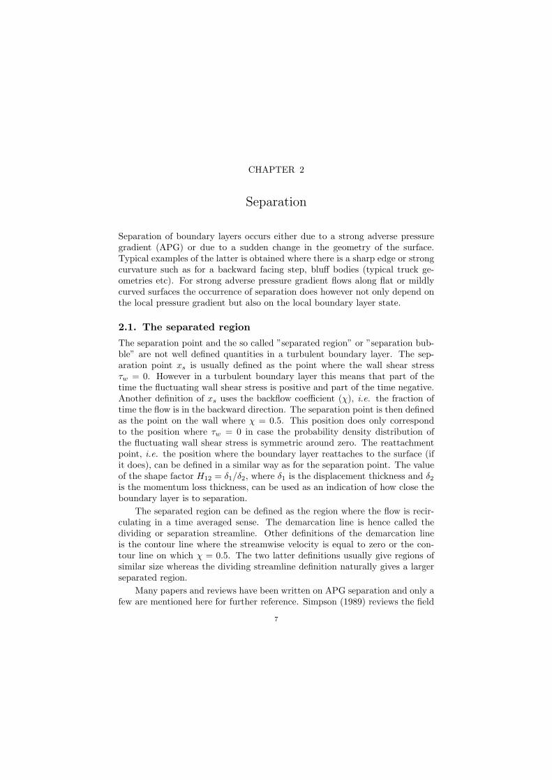
The three pressure gradients shown in figure 2.2(a) are compared in theexperiment. Case I is a weak separation bubble similar to the case of Dengel& Fernholz (1990), whereas case III is the strongest APG and the strengthof case II is approximately in between case I and case III. The separationbubble is here defined as the region where the backflow coefficient is χ > 0.5.Figure 2.2(b) shows the evolution of the shape factor in the three flow casesand figure 2.3 shows the separation bubble for case II. Upstream of x=1.8 m(before separation in all cases) there are no notable differences between thecases, but the maximum value of H12 in the separation bubble varies between4.1 for case I to more than 7 in case III. Furthermore, the value of H12 at thepoint of separation increases with the size of the separation bubble.

2.2. THE ZAGAROLA-SMITS VELOCITY SCALE 9

1 1.5 2 2.5 3

0

0.2

0.4

0.6

0.8

1

x (m)

Cp,

dC

p/d

x

1 1.5 2 2.5 30

2

4

6

8

H12

x (m)

(a) (b)

xhVG positions VG positions

Case IICase III

Case I

Figure 2.2. (a) The pressure distribution (Cp) and its gra-dient in the streamwise direction (dCp/dx). The region wherethe VGs are applied is indicated on the x-axis. (b) The shapefactor.

0 0 0 0 0 0 1.00

50

100

150

y (m

m)

x = 2.17 m x = 2.28 m x = 2.44 m x = 2.58 m x = 2.75 m x = 2.91 m

0.5 0.5 0.5 0.5 0.5 0.5U/Uinlet , χxs xr

hs

Figure 2.3. The separation bubble for the APG case II. Thefull lines show U/Uinlet, the dash-dotted lines show the back-flow coefficient χ. The separation bubble, defined as the regionwhere χ > 0.5, is the area below the lower dashed line. Theregion of χ > 0 is below the higher dashed line.

2.2. The Zagarola-Smits velocity scale

There is still no consensus on the proper mean velocity scaling of the outerregion in a strong APG and separated turbulent boundary layers. According toTownsend (1961), the criterion for similarity to exist in the mean velocity profileis that the ratio between the pressure gradient in the streamwise direction andτw is constant. This ratio is constant when H12 is constant. The validity of

10 2. SEPARATION

0 0.2 0.4 0.6 0.8 1 1.20

0.5

1

1.5

2

y/d95

(U - e

U)/U

ZS

Figure 2.4. Mean velocity profiles for case II. The top threesets of curves show velocity profiles upstream of separation(©), between the separation point and the position of themaximum in H12 () and after the maximum in H12 (4),respectively. The lower three curves show the average of theabove three sets.

Townsend’s criterion has been experimentally verified by Clauser (1954) andSkare & Krogstad (1994).

Turbulent boundary layers developing towards separation clearly do notfulfill this criterion, as τw decreases towards zero and then changes sign, whileH12 monotonically increases. Usually the friction velocity, uτ =

√τw/ρ is used

as the velocity scale. However to avoid the singularity at separation Mellor& Gibson (1966) suggested to instead use the scale up based on the pressuregradient and δ1. A different velocity scale, us, which explicitly depends on themaximum Reynolds shear-stress was suggested by Perry & Schofield (1973)and Schofield (1981). Here us is determined from a fit to the velocity profile.However Angele & Muhammad-Klingmann (2005a) showed that, for their data,up and us scale the same data-set upstream and downstream of separationequally well.

Recently, Maciel et al. (2006b) proved the usefulness of the Zagarola-Smitsvelocity scale (Zagarola & Smits (1998)), which is defined as

2.2. THE ZAGAROLA-SMITS VELOCITY SCALE 11

0 0.2 0.4 0.6 0.8 1 1.2

0

0.4

0.8

1.2

1.6

2

y/d95

x=2.10 m case IIIx=2.18 m case IIIx=2.24 m case IIIx=2.25 m case IIx=2.32 m case IIx=2.49 m case IIx=2.30 m case Ix=2.49 m case I

(U - e

U)/U

ZS

0

0.1

-0.1

Figure 2.5. Mean velocity profiles in the region between theseparation point and the position of the maximum in H12 forcases I, II and III. The insert shows how the velocity profilesdeviate from an average of all profiles. Note that the scale ofthe ordinate is increased in the insert.

UZS = Ueδ1δ, (2.1)

where Ue is the free-stream velocity and δ is the boundary layer thickness.Their data before and after separation show similarity for the outer layer meanvelocity distribution. Panton (2005) points out that uτ is proportional to theZagarola-Smits velocity scale for high Reynolds numbers. Maciel et al. (2006a)reviewed APG data from Perry (1966), Maciel et al. (2006b), Skare & Krogstad(1994), Dengel & Fernholz (1990) and others and showed that the Zagarola-Smits scaling works well.

In figure 2.4, the scaled mean velocity profiles of APG cases I-III are pre-sented in three sets: upstream of xs, in the separated region upstream of theposition of maximum in H12, denoted xh, and after the position of the maxi-mum in H12. In the region upstream of xs, the four plotted profiles do not showself-similarity. However, the three profiles between xs and xh are self-similarwhen scaled with UZS . The four velocity profiles for x > xh are also self-similar, but only within that set of profiles, i.e. they are not self-similar when

12 2. SEPARATION

they are plotted together with the profiles from upstream of xh, as is shownat the bottom of figure 2.4. Thus, there seem to be two different self-similarregions in the separated region: before and after xh.

To investigate whether the similarity holds between different sized separa-tion bubbles, velocity profiles from the region xs < x < xh for flow cases I,II and III are scaled by UZS and plotted together in figure 2.5. In the outerregion all profiles collapse, which is noteworthy since the differences in size ofthe separation bubbles are quite large.

In the recent study of Maciel et al. (2006a), it is shown that the mean-velocity defect profiles display self-similarity at some streamwise positions, butthat data from the different experiments do not collapse. They suggest thatthe reason is the difference in the pressure gradients. The present results onthe other hand, show velocity profiles that are self-similar in all three pressuregradient cases. Both the streamwise positions and the ranges of H12 differbetween the cases. Thus, it is rather the streamwise position relative to thepoint of separation and the bubble maximum that determines the similarity.

CHAPTER 3

Vane-type vortex generators

Control of separation of boundary layer flows can be achieved through differentapproaches. One common method, that has proved to be effective, is to intro-duce longitudinal vortices in the boundary layer. The vortices enhance mixingand transport high momentum fluid towards the wall.

The vortices are normally produced by vane-type VGs, i.e. short wingsattached to the surface with the wingspan in the wall-normal direction and setat an angle α towards the mean flow direction. Such devices are commonlyseen on the wings of commercial aircraft and their blade height (h) are oftenslightly larger than δ. The first experiments on conventional vane-type passiveVGs were reported by Taylor (1947).

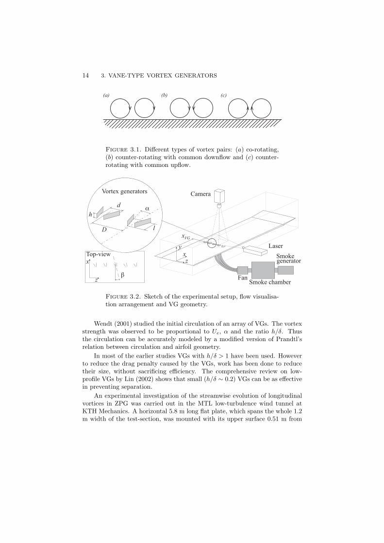
A VG array can be designed to produce different vortex configurations. Thethree basic types are shown in figure 3.1. The main geometrical parameters ofa VG array are shown in figure 3.2.

3.1. Vane-type VGs in ZPG

Pearcy (1961) published a comprehensive VG design guide. Here the vortextrajectories are also analysed, using the inviscid model from Jones (1957).

The evolution of a single vortices and vortex pairs embedded in a turbulentboundary layer was thoroughly investigated by Shabaka, Mehta & Bradshaw(1985) and later Mehta & Bradshaw (1988). They show that single vorticesproduce opposite sign vorticity around the vortex and that vortex pairs withcommon upflow are lifted out of the boundary layer. Another study of a singlevortex in a boundary layer was performed by Westphal, Pauley & Eaton (1987).The overall circulation, when the vortex evolved downstream, either decreasedslowly or remained almost constant depending on the case.

Pauley & Eaton (1988) examined the streamwise development of pairs andarrays of longitudinal vortices embedded in a zero pressure gradient (ZPG)turbulent boundary layer. In this study the blade spacing of VGs and theblade angle were varied, and the difference between counter-rotating vortices,with common upflow and downflow, and co-rotating vortices were examined.The proximity of other vortices does not affect circulation decay, but increasesthe diffusion of vorticity.

13

14 3. VANE-TYPE VORTEX GENERATORS

(a) (b) (c)

Figure 3.1. Different types of vortex pairs: (a) co-rotating,(b) counter-rotating with common downflow and (c) counter-rotating with common upflow.

d

h

D

α

xVG

Camera

Laser

Fan

xy

z

Vortex generators

l

βz

xTop-view Smoke

generator

Smoke chamber

Figure 3.2. Sketch of the experimental setup, flow visualisa-tion arrangement and VG geometry.

Wendt (2001) studied the initial circulation of an array of VGs. The vortexstrength was observed to be proportional to Ue, α and the ratio h/δ. Thusthe circulation can be accurately modeled by a modified version of Prandtl’srelation between circulation and airfoil geometry.

In most of the earlier studies VGs with h/δ > 1 have been used. Howeverto reduce the drag penalty caused by the VGs, work has been done to reducetheir size, without sacrificing efficiency. The comprehensive review on low-profile VGs by Lin (2002) shows that small (h/δ ∼ 0.2) VGs can be as effectivein preventing separation.

An experimental investigation of the streamwise evolution of longitudinalvortices in ZPG was carried out in the MTL low-turbulence wind tunnel atKTH Mechanics. A horizontal 5.8 m long flat plate, which spans the whole 1.2m width of the test-section, was mounted with its upper surface 0.51 m from

3.1. VANE-TYPE VGS IN ZPG 15

0

4

y/h

0

4

−0.5 0 0.50

4

z/D−0.5 0 0.5 −0.5 0 0.5

Figure 3.3. All three mean velocity components (from left toright, streamwise, wall-normal and spanwise) in the boundarylayer in the VGa

10 configuration. From top to bottom the rowscorrespond to (x− xVG)/h = 6, 42, and 167, respectively.

the test-section ceiling at the leading edge. The ceiling was adjusted to give azero streamwise pressure gradient at the nominal free stream velocity. At allvelocity measurements Ue was set to 26.5 m/s and the temperature was keptconstant at 18.1 C. The velocity measurements were performed using hot-wireX-probes with the anemometer operating in constant-temperature mode.

In order to set up the streamwise vortices inside the turbulent boundarylayer traditional vane-type VGs were used (see figure 3.2). Three different sizesof the VGs were used and arranged both as single spanwise pairs (p) as wellas spanwise arrays (a) to create counter-rotating vortices inside the boundarylayer. The design follows the criteria suggested by Pearcy (1961) and usesα = 15. The different VG sizes are geometrically ”self-similar”.

The vortices modify the base flow and in figure 3.3 the three mean velocitycomponents of the VG10 array configuration are contour plotted. The U - andW -components are symmetric, however the asymmetry in the V -component isdue to the large velocity gradients which affect the cooling velocities of the twowires of the X-probe differently. The maximum magnitude of the cross-flowcomponents are approximately 15-25 % of Ue in the measurement plane closestto the VG array.

In figure 3.4(a) the vortex centre paths from VG pairs are projected on they-z plane. The paths of the vortices behind the VGp

10 and the VGp18 seem to

collapse on each other. The downward motion in the beginning is caused bythe induced velocity by the neighbouring vortex. However, as the two vortices

16 3. VANE-TYPE VORTEX GENERATORS

0

1

2

3y/

h4

-0.4 -0.2 0 0.2 0.40

1

2

3

z/D

y/h

4

0.6-0.6

(a)

(b)

Figure 3.4. Vortex centre paths plotted in a y-zplane normalto the stream. (− · ♦ · −, —2—, − − © − −) denote VG6,VG10, and VG18, respectively. (a) The paths downstream ofa VG pair. (b) The same planes for an array of VGs .

move away from each other the influence from neighbouring vortex becomesweaker and the growth of the vortex causes the vortex centre to move awayfrom the wall. An interesting behaviour of the VGp

6 vortex path is that it turnsback towards the centre line.

The corresponding vortex paths of the VG arrays are shown in figure 3.4(b).In the case of the array, when the vortices move away from each other they aremoving closer to the vortex from the neighbouring vortex pair and eventuallyform a new counter-rotating pair – this time with common upflow. The inducedvelocities in the new pair will tend to lift the vortices and according to inviscidtheory (Jones 1957) they will continue to rise from the wall. However, themeasurements show that the vortex centre paths of the original pair, while stillrising, start to move towards each other again. This is probably due to vortexgrowth; when the area of the vortex grows the vortices are forced to a spanwiseequidistant state. The maximum vortex radius in an equidistant system ofcircular vortices is D/4, where D is the spanwise distance between the VGpairs. If the distance from the vortex centre to the wall is D/4 (2.08h), theinduced velocities from the real vortices and the three closest mirrored vortices

3.1. VANE-TYPE VGS IN ZPG 17

x/h

50 100 150 200 250 300

-0.4

0

0.4

(x-x ) /h

z/D

0

-0.4

0

0.4z/

D

(a)

(b)

VG

Figure 3.5. Vortex centre paths plotted in plan view (the x-z plane). (− · ♦ · −, —2—, − −© − −) denote h = (6, 10,18) mm. (a) The paths downstream of a pair of VGs. (b) Thesame planes for a VG array. Note that for the array the pathsof the neighboring vortices are actually within the figure area,but for the sake of clarity they are not shown.

all cancel. Hence, if the assumption holds, the vortex centres should approach(y/h, z/D) = (2.08,±0.25). In figure 3.4(b), these coordinates are markedwith small circles, and there seem to be a tendency for the vortex centres tomove towards the predicted position.

Now, it is possible to explain the peculiar vortex centre path produced bythe VGp

6 in figure 3.4(a). In analogy to the paths of the vortices generatedby the array, the curving back motion indicates the existence of secondaryvortices, outside of the primary pair. At (x− xVG)/h = 445 the circulation ofthe secondary vortices is about 55 % of the primary vortices. The secondaryvortices probably originate from the very thin layer of stress-induced opposingωx under the primary vortex.

In figure 3.5(a) the vortex paths from the single VG pair are shown in planview. A divergence of the paths, from all VG sizes, caused by the mirroredimages can be observed. The angle of divergence increases with vortex strength.Vortex centre paths downstream of VG arrays are plotted in figure 3.5(b). Inplan view it is easy to see how the paths first move apart, roughly at the samerate as in the case of the single pairs, up to about (x− xVG)/h = 50 and then

18 3. VANE-TYPE VORTEX GENERATORS

0 100 200 300 400 500−5

0

5

10

15x 10−3

u iu j/Ue2

0 100 200 300 400 500−5

0

5

10

15x 10−3

(a) (b)

(x-x )/hVG (x-x )/hVG

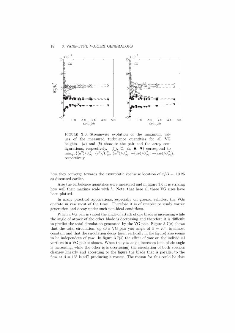
Figure 3.6. Streamwise evolution of the maximum val-ues of the measured turbulence quantities for all VGheights. (a) and (b) show to the pair and the array con-figurations, respectively. (©, 2, 4, , H) correspond tomaxyz〈u2〉/U2

∞, 〈v2〉/U2∞, 〈w2〉/U2

∞, −〈uv〉/U2∞, −〈uw〉/U2

∞,respectively.

how they converge towards the asymptotic spanwise location of z/D = ±0.25as discussed earlier.

Also the turbulence quantities were measured and in figure 3.6 it is strikinghow well their maxima scale with h. Note, that here all three VG sizes havebeen plotted.

In many practical applications, especially on ground vehicles, the VGsoperate in yaw most of the time. Therefore it is of interest to study vortexgeneration and decay under such non-ideal conditions.

When a VG pair is yawed the angle of attack of one blade is increasing whilethe angle of attack of the other blade is decreasing and therefore it is difficultto predict the total circulation generated by the VG pair. Figure 3.7(a) showsthat the total circulation, up to a VG pair yaw angle of β = 20, is almostconstant and that the circulation decay (seen vertically in the figure) also seemsto be independent of yaw. In figure 3.7(b) the effect of yaw on the individualvortices in a VG pair is shown. When the yaw angle increases (one blade angleis increasing, while the other is is decreasing) the circulation of both vorticeschanges linearly and according to the figure the blade that is parallel to theflow at β = 15 is still producing a vortex. The reason for this could be that

3.2. VANE-TYPE VGS IN APG 19

0

0.5

1

1.5

0 4 8 12 16 20β (deg)

qhU

VG

Γ Total circulationStrong vortexWeak vortex

0 4 8 12 16 20β (deg)

(a) (b)

Figure 3.7. (a) The total circulation, i.e. the contributionfrom both the vortices, in the VGp

10 case versus the yaw angleat (x−xVG)/h = 6, 41, 116 shown by (, 2, ♦), respectively.(b) The individual contribution from the two vortices for theVGp

10 case at (x− xVG)/h = 6.

the strong vortex is deflecting the flow to reach the parallel blade at some angleor that this is caused by vorticity induced by the larger vortex.

3.2. Vane-type VGs in APG

Much research on VGs have been done in ZPG, but their real use is in APG.Schubauer & Spangenberg (1960) tried a variety of wall mounted devices toincrease the mixing in the boundary layer. They did this in different APGsand they concluded that the effect of mixing is equivalent to a decrease inpressure gradient.

Godard & Stanislas (2006) made an optimisation study on co- and counter-rotating VGs submerged in a APG boundary layer. They found that thecounter-rotating set-up was twice as effective as the co-rotating in increasingthe wall shear stress. In another recent experiment Angele & Muhammad-Klingmann (2005a) made extensive PIV measurements to show the flow andvortex development inside a turbulent boundary layer with a weak separationbubble.

In the present study the VG arrays of section 3.1 were positioned upstreamof the separation bubbles described in section 2.1. Due to the rapidly growingboundary layer in that region, which causes the velocity at y = h to vary,four different VG arrays could be used to produce any vortex strength up toγe

1 = 4.0 m/s by placing them at different streamwise positions (xVG). Theeffect of the VGs on the separated region was studied with PIV.

1γe is the circulation per unit width, calculated from h and the velocity at y = h.

20 3. VANE-TYPE VORTEX GENERATORS

-0.1 0 0.1 0.3 0.5 0.7 0.90

50

100

150

U/Ue

y (m

m)

γ = 3.8γ = 3.1γ = 1.4γ = 1.0γ = 0.8γ = 0

eeeeee

-0.1 0 0.1 0.3 0.5 0.7 0.9U/Ue

(a) (b)

Figure 3.8. Mean velocity profiles at (a) the spanwise posi-tion of inflow and (b) the position of outflow.

In figure 3.8 the streamwise mean velocity profiles at the positions of inflowand outflow are shown for different VG configurations at xh in APG case II.The uncontrolled case is shown for comparison. At the position of inflow, morestreamwise momentum is transported down, and a larger effect of the VGscan be seen. The two VGs which produce the smallest amount of circulationhave negligible influence on U , but when the circulation is increased to γe =1.4 separation is prevented. This is the most efficient VG configuration foreliminating separation in this particular flow case, in the sense that the draggenerated by the VGs is expected to be less than that generated by the largerVGs. Even though this gives a pronounced efficiency maximum it could alsocause a system designed for maximum efficiency to be sensitive to changes inthe flow conditions.

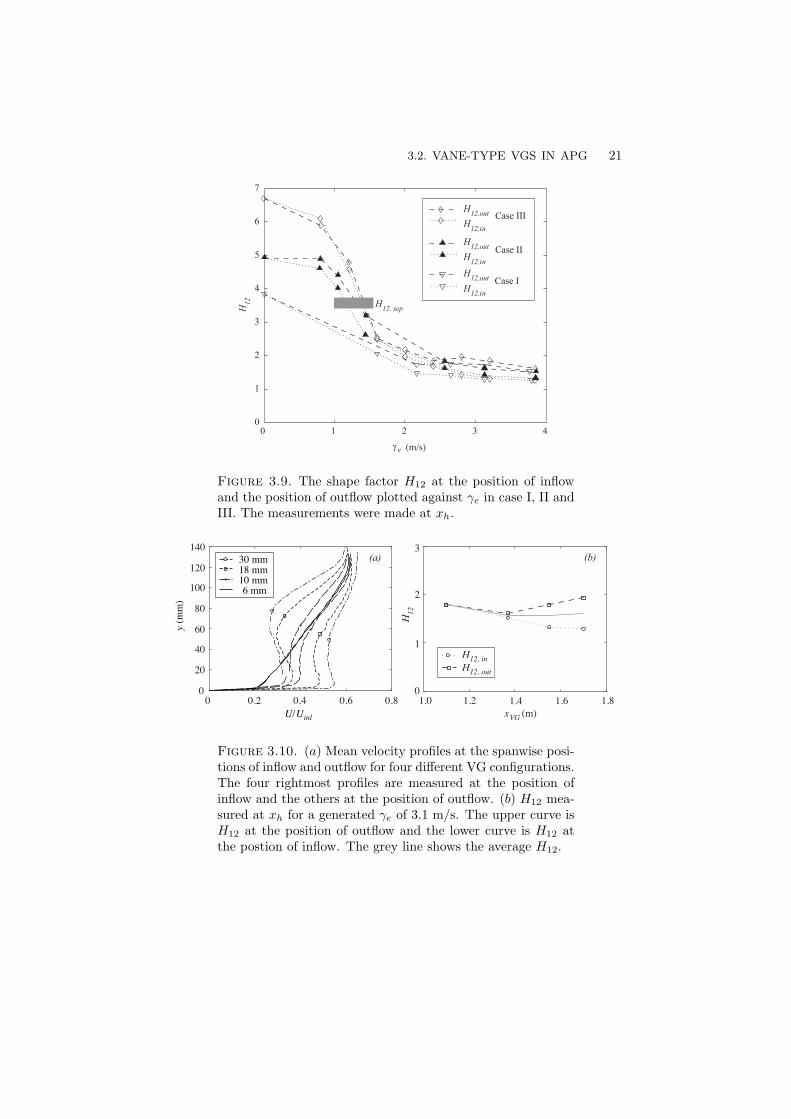
Figure 3.9 summarizes the separation control effectiveness, in terms of H12,of all examined VG configurations. Here H12 at xh for cases I, II and III arecompared for different magnitudes of γe. In the uncontrolled case, H12 is about4, 5 and 7 in the respective cases. The value of γe at which the flow staysattached seems to be fairly insensitive to the pressure gradient, even thoughthe difference in size of the separated region is quite large in the uncontrolledcases. When γe is further increased, the average H12 seems to asymptoticallyapproach 1.4, which is the value of a ZPG turbulent boundary layer.

In order to investigate the influence of xVG, the same level of circulationwas produced at four different x positions. This was accomplished by ap-plying differently sized VGs at different streamwise positions so that Uh aty = h is constant. Two arrays are placed before the pressure gradient peak,one is placed at the peak-position and one is positioned right after the maxi-mum. In figure 3.10(a) the resulting mean streamwise velocity profiles at xh

3.2. VANE-TYPE VGS IN APG 21

0 1 2 3 4 0

1

2

3

4

5

6

7

H12

H12,in

H12,out

H12,in

H12,out

H12,in

H12,out

γ (m/s)e

Case II

Case III

Case I

H12, sep

Figure 3.9. The shape factor H12 at the position of inflowand the position of outflow plotted against γe in case I, II andIII. The measurements were made at xh.

0

1

2

3

H12

xVG

1.0 1.2 1.4 1.6 1.8 (m)

H12, inH12, out

0 0.2 0.4 0.6 0.80

20

40

60

80

100

120

14030 mm18 mm10 mm6 mm

U/Uinl

y (m

m)

+

++

(a) (b)

Figure 3.10. (a) Mean velocity profiles at the spanwise posi-tions of inflow and outflow for four different VG configurations.The four rightmost profiles are measured at the position ofinflow and the others at the position of outflow. (b) H12 mea-sured at xh for a generated γe of 3.1 m/s. The upper curve isH12 at the position of outflow and the lower curve is H12 atthe postion of inflow. The grey line shows the average H12.

22 3. VANE-TYPE VORTEX GENERATORS

are presented. For the case of 6 mm high VGs the boundary layer seems two-dimensional, but the 10 mm VG array shows a fuller profile at the position ofinflow. For the next two cases of larger VGs, the shift of the profiles increases.However, if an average of the profiles at the inflow and outflow positions istaken for each VG size, the curves of the three largest VGs are similar. Hence,the shape factor of the average mean velocity profiles will be similar. Thisis shown in figure 3.10(b), where H12 at the inflow and outflow positions areplotted versus the upstream distance to the VG arrays. From this figure onecan conclude that H12 at xh, i.e. the control effect, is quite insensitive to thestreamwise position of the VGs.

CHAPTER 4

Jet vortex generators

An alternative way of producing the vortices is by jets originating from thewall. Flow control by vortex generator jets (VGJs) was first described by Wallis(1952). He claimed that an array of VGJs could be as effective as passive VGsin suppressing separation on an airfoil. In the following the jet direction is givenby the skew and pitch angle, see figure 4.1 for a definition of the geometry.

4.1. Steady jet VGs

A study by Johnston & Nishi (1990) demonstrated how streamwise vortices areproduced by a VGJ array. A pitch angle of less than 90 was needed in order togenerate vortices effectively. Some success in reducing the size of a separatedregion in an APG, was also demonstrated when the velocity ratio VR, whichis the ratio of jet speed to free stream velocity, was 0.86 or higher. Compton& Johnston (1992) studied VGJs pitched at 45. A skew between 45 and 90

was found to give the strongest vortices. The circulation of the vortices wasalso found to increase as the VR was increased.

In a study on a backward facing 25 ramp, where the flow separates, Selby,Lin & Howard (1992) measured the pressure for different VGJ array configu-rations. The pressure recovery increased up to the highest tested VR ratio of6.8. It was shown that a small pitch angle (15 or 25) is beneficial and thatthe optimum skew angle appears to be between 60 and 90.

According to the review by Johnston (1999) the VR is the dominant pa-rameter in generating circulation. The exact streamwise location of the VGJrow seems less important since the boundary layer reacts likewise independentof where it is energised. Khan & Johnston (2000) performed detailed measure-ments downstream of one VGJ and showed that the flow field is similar to thatof solid VGs.

Zhang (2000) showed that a rectangular jet can produce higher levels ofvorticity and circulation compared to a circular jet of equal hydraulic diameterand VR. Another experiment on the jet orifice shape by Johnston, Moiser &Khan (2002) showed that the inlet geometry affects the near-field but not thefar-field. Zhang (2003) studied co-rotaing vortices produced by a spanwise arrayof VGJs, where both skew and pitch are set to 45, and described the complex

23

24 4. JET VORTEX GENERATORS

U

y

z

x

Side-view

Top-view

β

α Ujet

Ujet

z

α

βL

λ

U

d

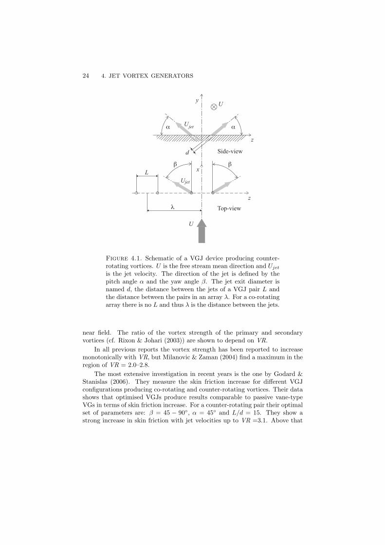
Figure 4.1. Schematic of a VGJ device producing counter-rotating vortices. U is the free stream mean direction and Ujetis the jet velocity. The direction of the jet is defined by thepitch angle α and the yaw angle β. The jet exit diameter isnamed d, the distance between the jets of a VGJ pair L andthe distance between the pairs in an array λ. For a co-rotatingarray there is no L and thus λ is the distance between the jets.

near field. The ratio of the vortex strength of the primary and secondaryvortices (cf. Rixon & Johari (2003)) are shown to depend on VR.

In all previous reports the vortex strength has been reported to increasemonotonically with VR, but Milanovic & Zaman (2004) find a maximum in theregion of VR = 2.0–2.8.

The most extensive investigation in recent years is the one by Godard &Stanislas (2006). They measure the skin friction increase for different VGJconfigurations producing co-rotating and counter-rotating vortices. Their datashows that optimised VGJs produce results comparable to passive vane-typeVGs in terms of skin friction increase. For a counter-rotating pair their optimalset of parameters are: β = 45 − 90, α = 45 and L/d = 15. They show astrong increase in skin friction with jet velocities up to VR =3.1. Above that

4.1. STEADY JET VGS 25

Accumulator tank 2

Precisionregulator

Indicator jet

HW anemometer

VGJ array

Power supply Control computer

Fast-switching valve

x = 1.50 m x = 2.55 m

Measurement plane

Approximate separation line

Figure 4.2. Schematic of VGJ set-up.

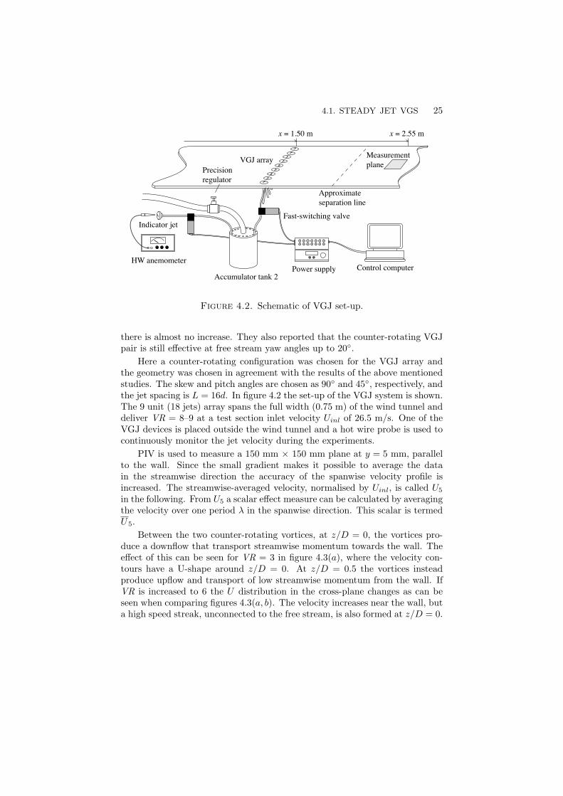
there is almost no increase. They also reported that the counter-rotating VGJpair is still effective at free stream yaw angles up to 20.

Here a counter-rotating configuration was chosen for the VGJ array andthe geometry was chosen in agreement with the results of the above mentionedstudies. The skew and pitch angles are chosen as 90 and 45, respectively, andthe jet spacing is L = 16d. In figure 4.2 the set-up of the VGJ system is shown.The 9 unit (18 jets) array spans the full width (0.75 m) of the wind tunnel anddeliver VR = 8–9 at a test section inlet velocity Uinl of 26.5 m/s. One of theVGJ devices is placed outside the wind tunnel and a hot wire probe is used tocontinuously monitor the jet velocity during the experiments.

PIV is used to measure a 150 mm × 150 mm plane at y = 5 mm, parallelto the wall. Since the small gradient makes it possible to average the datain the streamwise direction the accuracy of the spanwise velocity profile isincreased. The streamwise-averaged velocity, normalised by Uinl, is called U5

in the following. From U5 a scalar effect measure can be calculated by averagingthe velocity over one period λ in the spanwise direction. This scalar is termedU5.

Between the two counter-rotating vortices, at z/D = 0, the vortices pro-duce a downflow that transport streamwise momentum towards the wall. Theeffect of this can be seen for VR = 3 in figure 4.3(a), where the velocity con-tours have a U-shape around z/D = 0. At z/D = 0.5 the vortices insteadproduce upflow and transport of low streamwise momentum from the wall. IfVR is increased to 6 the U distribution in the cross-plane changes as can beseen when comparing figures 4.3(a, b). The velocity increases near the wall, buta high speed streak, unconnected to the free stream, is also formed at z/D = 0.

26 4. JET VORTEX GENERATORS

0.30.32 0.320.34

0.36

0.38

0.4

0.420.44

0.46y

(mm

)

0

20

40

60

0.38 0.380.4 0.40.42

0.44

0.46 0.46

0.460.48

0.48

0.5z/D

−0.5 0 0.5z/D

−0.5 0 0.5

(a) (b)

Figure 4.3. Contours of (a) U/Uinl at VR = 3, (b) U/Uinlat VR = 6. All measurements are taken at xh.

−0.5 0 0.5−0.1

0

0.1

0.2

0.3

0.4

z/D0 2 4 6 8

−0.1

0

0.1

0.2

0.3

0.4

VR

U5

(a) (b)

U 5

Figure 4.4. (a) Velocity profiles at y = 5 mm for differentVR and (b) the corresponding mean velocities U5.

With a fixed geometry the only variable parameter of the VGJs is VR.In figure 4.4(a) the velocity profiles at different jet velocities are shown andin figure 4.4(b) the corresponding U5 is shown. There is almost no changewhen the jets are activated at VR = 0.5. This is possibly because the jets arestill too weak to produce any vortices. A further velocity increase to VR = 1.0eliminates the mean backflow. Thus, there are now longitudinal vortices presentin the boundary layer. From VR = 0.5 to VR = 2.0 the increase in U5 withVR is nearly linear. After that and up to VR = 5.0 the control effectiveness isstill increasing, but at a lower rate. Above VR = 5.0 there is a decrease in U5.

The VGJ array is also tested at yaw. The VGJ devices of the array areyawed individually, at θ = 0−90, and the resulting U5 is shown in figure 4.5.U5 decreases slowly with θ, down to a minimum at θ = 60. For increasing θ >

4.2. PULSED JET VGS 27

0 20 40 60 80

0

0.1

0.2

0.3

0.4

θ ( )

U5

Figure 4.5. Effectiveness at different yaw angles. The opencircles show VR = 3 and the filled circles show VR = 5.

60 U5 increases to a second maximum at θ = 90. This is more pronouncedfor VR = 5

4.2. Pulsed jet VGs

The flow control effect of pulsed VGJs can be due to several different physicalmechanisms. They can influence the flow by amplifying natural frequencies inthe boundary layer, like the shedding of a stalled airfoil. Furthermore, theycan function like steady VGJs and produce longitudinal vortices that transporthigh momentum fluid towards the wall. In the experiment presented in thisarticle pulsed VGJs of the last category are applied. If the VGJ geometry isset, there are three main parameters that decide the performance of a pulsedVGJ. It is the velocity ratio, the pulsing frequency f and the duty cycle Ω.

For steady VGJs the generated circulation depend strongly on VR and thesame is valid for for pulsed VGJs. This has been shown for arrays of VGJs byMcManus et al. (1995) and Kostas et al. (2007). Also similar to steady jetsis the occurrence of an circulation optimum in VR above which the vortex istranslated out of the boundary layer.

In McManus et al. (1995) and Scholz et al. (2008) the frequency had littleeffect on lift and drag, but in McManus et al. (1996) the magnitude of theupper side suction peak was strongly dependent on the pulsing frequency. Theoptimum frequency Strouhal number was found to be of the same order as thatcharacterizing the natural eddy shedding behind blunt objects.

The duty cycle was shown by Scholz et al. (2008) to be important in in-creasing post-stall lift on an airfoil. They found Ω ≤ 0.25 to be most beneficial.

28 4. JET VORTEX GENERATORS

0 0.5 1 1.5 2 2.5 30

1

2

3

4

t/T

VR t1 T

Figure 4.6. Jet pulses at VR = 3 and f = 100 Hz. The datais averaged over 30 cycles.

0 2 4 6 8−0.1

0

0.1

0.2

0.3

0.4

VR, VR

U5

*10−4 10−3 10−2 10−10

0.05

0.1

0.15

0.2

Stjet

U 5/V

R∗

Figure 4.7. (a) U5 vs VR and VR∗. The full line show steadyjet results, the dashed line show average pulsed jet results andthe symbols indicate U5 vs VR∗. (b) U5/VR

∗ vs Stjet at VR =2, 3 and 4.

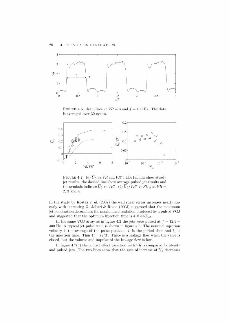
In the study by Kostas et al. (2007) the wall shear stress increases nearly lin-early with increasing Ω. Johari & Rixon (2003) suggested that the maximumjet penetration determines the maximum circulation produced by a pulsed VGJand suggested that the optimum injection time is 4–8 d/Ujet.

In the same VGJ array as in figure 4.2 the jets were pulsed at f = 12.5−400 Hz. A typical jet pulse train is shown in figure 4.6. The nominal injectionvelocity is the average of the pulse plateau. T is the period time and t1 isthe injection time. Thus Ω = t1/T . There is a leakage flow when the valve isclosed, but the volume and impulse of the leakage flow is low.

In figure 4.7(a) the control effect variation with VR is compared for steadyand pulsed jets. The two lines show that the rate of increase of U5 decreases

4.2. PULSED JET VGS 29

0 0.5 1.0−0.1

0

0.1

0.2

0.3

0.4

Ω

U5

Δ

0 500 1000

0.15

0.2

0.25

t1+

U5

/VR∗

Increasing Ω

Figure 4.8. (a) U5 vs Ω for f = 12.5 Hz (), f = 25 Hz(), f = 50 Hz (), f = 100 Hz (4) and f = 200 Hz (O) atVR = 3. (b) ∆U5/VR

∗ vs t+1 for the same data as in (a)

at VR ≈ 2.5− 3 for both configurations. The symbols show the data points atdifferent frequencies and VRs plotted against VR∗ = ΩVR. When the pulseddata is compensated for the lower mass flow by using VR∗ as measure, thecontrol effect is similar to that of the steady jets. In order to study whetherthere is an maximum volume efficiency, the control effect is recalculated asU5/VR

∗. If U5/VR∗ is plotted against the jet based Strouhal number Stjet =

fd/Ujet, there seems to be an optimum, as can be seen in figure 4.7(b).The frequency and Ω were varied at a constant VR = 3. In figure 4.8(a)

the resulting U5 is shown. Compared to Ω, the influence of f is small. A non-dimensional injection time is defined as t+1 = t1Ujet/d, and the variation of thecontrol efficiency ∆U5/VR

∗ with t+1 is shown in figure 4.8(b). There seems tobe a maximum at t+1 = 100− 200

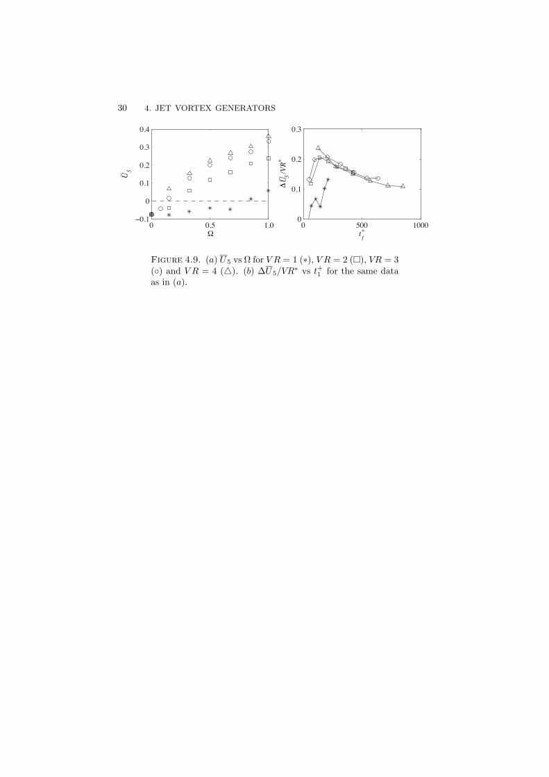
At a constant f = 50 Hz, the VR and Ω is varied. As expected, figure 4.9(a)shows that a higher velocity ratios and longer duty cycles produce more controleffect. If instead, the variation of ∆U5/VR

∗ with t+1 is studied, as shown infigure 4.9(b), it is possible to identfy a maximum at t+1 = 100−150 for VR = 2, 3and 4.

30 4. JET VORTEX GENERATORS

0 0.5 1.0−0.1

0

0.1

0.2

0.3

0.4

Ω

U5

Δ

0 500 10000

0.1

0.2

0.3

t1+

U5

/VR∗

Figure 4.9. (a) U5 vs Ω for V R = 1 (∗), V R = 2 (), VR = 3() and V R = 4 (4). (b) ∆U5/VR

∗ vs t+1 for the same dataas in (a).

CHAPTER 5

Conclusions

In this chapter the main conclusions from the different investigations are sum-marised.

5.1. The separated region• In the separated region the Zagarola-Smits velocity scaling was found

to better scale the mean-velocity defect profiles than the methods sug-gested by Mellor & Gibson (1966), Perry & Schofield (1973) and Schofield(1981).

• There were two regions of similarity: before and after the maximumof H12 and χw in the separation bubble. In these two regions velocitydefect profiles are independent of the pressure gradient.

• H12 increases linearly with increasing χw in the separated region. Down-stream of their maxima, H12 decreases linearly with decreasing χw, butat a higher level of H12.

5.2. Vane-type VGs• The vortex core paths in plan view as well as in the plane normal to the

flow, scale with the VG size in the downstream and spanwise directions.• In this paper an asymptotic limit hypothesis of the vortex array path

is stated and is shown to hold reasonable well. The limiting valuesfor vortices far downstream are (y/h, z/D) = (2.08,±0.25), which theexperimental data seems to approach.

• It is here shown, in the VG pair case, that the vortices are able to induceopposite sign vorticity, which is rolled up into a secondary vortex andstrongly affect the primary vortex path.

• For VG arrays of different sizes, but with self-similar geometry, thegenerated circulation increases linearly with the vane tip velocity.

• In both the pair and the array configurations, the circulation decaysexponentially at approximately the same rate.

• The maxima of the turbulence quantities scale with h in the streamwisedirection.

• The spanwise-averaged shape factor and circulation are unaffected byyaw.

31

32 5. CONCLUSIONS

• In order to capture the evolution of vortex core paths in the far regionbehind an array of counter-rotating vortices it has been shown througha pseudo-viscous vortex model that circulation decay and streamwiseasymptotic limits have to be taken into account.

• For three separation bubbles of different size, separation was preventedat approximately the same λe. For higher λe, H12 for all APGs approacha asymptotic value of 1.4.

• The streamwise position of the vortex generating devices is, within acertain range, of minor importance, which makes separation control byVGs robust and less sensitive to changing boundary conditions.

5.3. Jet VGs• VGJs have been shown to be as effective as vane-type VGs. Further-

more, there seems to be a maximum possible value of U5 ≈ 0.4, that iscommon for both systems.

• The maximum U5 is reached at VR = 5. The maximum volume flowefficiency and the maximum kinetic energy efficiency is obtained atVR = 2.0 and VR = 1.0, respectively.

• At yaw the control effect is decreasing slowly up to θ = 40, where itis still 70–80 % of the non-yawed level. Thus, the system robustness foryaw is good.

• When VR is in the maximum efficiency range and more control isneeded, the VGJ array should, if possible, be made denser instead ofincreasing VR. Similarly, to reduce control the VGJ array is made moresparse.

• The basic mechanism of pulsed VGJs is pulse-width modulation. Thecontrol effectiveness is primarily a function of VR∗ = ΩVR. Thus, formaximum effectiveness at constant VR the duty cycle should be Ω = 1.

• If they can be run at the optimum VR, pulsed jets can be more efficientthan steady jets for a required level of U5.

• For a given Ω there is a optimum Stjet. The optimum Stjet can be seenas a limit for a robust system, due to the rapid decrease in control effectat frequencies higher than the optimum.

• The injection time, and not Ω, is the relevant parameter. Here theoptimal injection time span is 100 < t+1 < 200. The optimum Stjetmentioned above can be expressed in t+1 . Thus, there are only twonon-geometry parameters that determine the efficiency: VR and t+1 .

• Johari & Rixon (2003) suggested that the optimal injection time forpulsed VGJs is in the range of 4–8 d/Ujet. In the present experimentthe optimal t1 has been shown to be approximately 25 times longer.

CHAPTER 6

Outlook

6.1. Practical applications

Flow control systems utilising vane-type VGs, steady VGJs or pulsed VGJshave been shown to be effective and robust. This make them suitable for useon ground vehicles. As mentioned earlier an array can be utilised to energisethe boundary layer upstream of a steep tapering of the vehicle rear end and thusprevent separation. The effectiveness of VGs and VGJs are equal and thereforethe choice can be based on which system is the most practical. Passive VGsare of course simpler, but sharp blades cannot be mounted on a ground vehicledue to safety reasons. Furthermore they can not be turned off while brakingor when driving in a convoy1.

There are other areas on a ground vehicle that can benefit from flow control,as for example the underbody. The internal flow systems can also be improved.The air inlet to the engine should have a low pressure drop even though thepipes are bent. Also the important cooling air flow can be increased if thepressure drop is reduced.

An obvious application of VGJs is on airplanes. Vane-type VGs are alreadyused on wings and in engine air intakes, however also on an airplane it is usefulto be able to turn of the flow control system.

6.2. Further research

There are two main areas of interest that needs to be pursued: the applicationof the VGJ system on a bluff body and the exchange of pulsed jets for syntheticjets.

It would be valuable to study the effect of VGJs on a truck-like bluff bodyand analyse how the energy consumption will change. If the energy consump-tion of the jets is larger than the decrease in energy consumption caused bythe drag reduction the system is less useful.

Synthetic jets are very attractive since they require no air supply and thusmake the installation simple. Since a synthetic jet has little influence on theboundary layer during its suction phase their flow control mechanisms are the

1The total drag of a convoy of trucks can probably be reduced if all vehicles except the last

turn off their flow control systems to increase the wake size.

33

34 6. OUTLOOK

same as for non-synthetic jets. One example of a study using synthetic jets isthe investigation by Amitay et al. (2001). Synthetic jets are probably the wayahead, but injection times in the order of 100–200 d/Ujet requires actuatorswith large reservoirs.

CHAPTER 7

Papers and authors contributions

Paper 1On the scaling of turbulent boundary layers.Ola Logdberg (OL), K. P. Angele (KA) & P. H. Alfredsson (HAL).Phys. Fluids 20, 075104, 2008.

The experiments on APG case I was performed by KA and has already beenreported in Angele & Muhammad-Klingmann (2006). APG cases II and IIIwere measured by OL. The data analysis was done by OL and the writing wasdone by OL and KA jointly, in cooperation with HAL.

Paper 2Streamwise evolution of longitudinal vortices in a turbulent boundary layer.Ola Logdberg, J. H. M. Fransson (JF) & P. H. Alfredsson.J. Fluid Mech. (In press).

The experiment was set up by OL, under the supervision of JF. The experi-ments and the data analysis were performed by OL. The writing was done byOL and JF jointly, in cooperation with HAL. Parts of this work was presentedat the 6th European Fluid Mechanics Conference 2006, Stockholm. Some ofthe results have also been reported in Stillfried, Logdberg, Wallin & Johansson(2009).

Paper 3On the robustness of separation control by streamwise vortices.Ola Logdberg, K. P. Angele & P. H. Alfredsson

The experiments on APG case I was performed by KA and has already beenreported in Angele & Muhammad-Klingmann (2005a). APG cases II and IIIwere measured by OL. The data analysis was done by OL and the writingwas done by OL, in cooperation with KA and HAL. Parts of this work waspresented at the 4th International Symposium of Turbulence and Shear FlowPhenomena 2005, Williamsburg.

35

36 7. PAPERS AND AUTHORS CONTRIBUTIONS

Paper 4Separation control by an array of vortex generator jets. Part 1. Steady jets.Ola Logdberg

Paper 5Separation control by an array of vortex generator jets. Part 2. Pulsed jets.Ola Logdberg

37

Acknowledgements

First I would like to thank my supervisor Prof. Henrik Alfredsson for acceptingme as his student and for his guidance.

I would also like to thank my assistant supervisor Dr. Jens Fransson forteaching me how to set up and perform a nice experiment. Everything is somuch easier if you are well organised.

Furthermore, I would like to thank Dr. Kristian Angele for introducing meto PIV and for his unlimited enthusiasm.

Special thanks to Dr. Olle Tornblom, Tek. Lic. Timmy Sigfrids andDr. Claes Holmqvist for sharing lots of practical and theoretical knowledgeon fluid mechanics. Thanks to Thomas Kurian for helping me with X-probesoldering. Tek. Lic. Ramis Orlu also assisted me with my probes, but he isalso acknowledged for being the most helpful person in the lab. Thanks to Dr.Nils Tillmark for nice discussions and for his quest to bring some order to thelab.

I would like to thank my office-mates Dr. Thomas Hallqvist, Bengt Fall-enius and Malte Kjellander for providing a cosy atmosphere. I also thank allother colleagues in lab for being nice and helpful.

Marcus Gallstedt, Ulf Landen, Joakim Karlstrom and Goran Radberg inthe work shop are all highly acknowledged for good advice and help with myexperimental set-ups.

Scania CV AB is acknowledged for giving me the opportunity to carry outmy doctorial work at KTH Mechanics within the Linne Flow Centre. Manythanks to Per Jonsson and Dr. Per Elofsson for their support.

Tack Cecilia! Livet vore sa mycket trakigare utan dig.

38

References

Amitay, M., Smith, D., Kibens, V., Parekh, D. E. & Glezer, A. 2001 Aerody-namic flow control over an unconventional airfoil using synthetic jet actuators.AIAA J. 39, 361–370.

Angele, K. P. & Muhammad-Klingmann, B. 2005a The effect of streamwise vor-tices on the turbulence structure of a separating boundary layer. Eur. J. Mech.B 24, 539–554.

Angele, K. P. & Muhammad-Klingmann, B. 2005b A simple model for the effectof peak-locking on the accuracy of boundary layer statistics in digital PIV. Exp.Fluids 38, 341–347.

Angele, K. P. & Muhammad-Klingmann, B. 2006 PIV measurements in a weaklyseparating and reattaching turbulent boundary layer. Eur. J. Mech. B 25, 204–222.

Clauser, F. 1954 Turbulent boundary layers in adverse pressure gradients. J. Aero.Sci. 21, 91–108.

Compton, D. & Johnston, J. 1992 Streamwise vortex production by pitched andskewed jets in a turbulent boundary layer. AIAA J. 30, 640–647.

Dengel, P. & Fernholz, H. 1990 An experimental investigation of an incompress-ible turbulent boundary layer in the vicinity of separation. J. Fluid Mech. 212,615–636.

Godard, G. & Stanislas, M. 2006 Control of a decelerating boundary layer. Part1: Optimization of passive vortex generators. Aero. Sci. Tech. 10, 181–191.

Godard, G. & Stanislas, M. 2006 Control of a decelerating boundary layer. part3: Optimization of round jets vortex generators. Aero. Sci. Tech. 10, 455–464.

Johari, H. & Rixon, G. S. 2003 Effects of pulsing on a vortex generator jet. AIAAJ. 41, 2309–2315.

Johnston, J. & Nishi, M. 1990 Vortex generator jets, means for flow separationcontrol. AIAA J. 28, 989–994.

Johnston, J. 1999 Pitched and skewed vortex generator jets for control of turbulentboundary layer separation: a review. In 3rd ASME/JSME Joint Fluids Eng.Conf.

Johnston, J., Moiser, B. & Khan, Z. 2002 Vortex generating jets; effects of jet-hole inlet geometry. Int. J. Heat Fluid Flow 23, 744–749.

39

40 REFERENCES

Jones, J. P. 1957 The calculation of the paths of vortices from a system of vor-tex generators, and a comparison with experiment. Tech Rep. C. P. No. 361.Aeronautical Research Council.

Kalter, M. & Fernholz, H. H. 2001 The reduction and elimination of a closedseparation region by free-stream turbulence. J. Fluid Mech. 446, 271–308.

Khan, Z. U. & Johnston, J. 2000 On vortex generating jets. Int. J. Heat FluidFlow 21, 506–511.

Kostas, J., Foucaut, J. M. & Stanislas, M. 2007 The flow structure produced bypulsed-jet vortex generators in a turbulent boundary layer in an adverse pressuregradient. Flow, Turbul. Combust. 78, 331–363.

Lin, John C. 2002 Review of research on low-profile vortex generators to controlboundary-layer separation. Prog. Aero. Sci. 38, 389–420.

Maciel, Y., Rossignol, K.-S. & Lemay, J. 2006a Self-similarity in the outer regionof adverse-pressure-gradient turbulent boundary layers. AIAA J. 44, 2450–2464.

Maciel, Y., Rossignol, K.-S. & Lemay, J. 2006b A study of a turbulent boundarylayer in stalled-airfoil-type flow conditions. Exp. Fluids 41, 573–590.

McManus, K., Joshi, P., Legner, H. & Davis, S. 1995 Active control of aerody-namic stall using pulsed jet actuators, AIAA paper 95-2187 .

McManus, K., Ducharme, A., Goldey, C. & Magill, J. 1996 Pulsed jet actua-tors for surpressing flow separation, AIAA paper 96-0442 .

Mehta, R. D. & Bradshaw, P. 1988 Longitudinal vortices imbedded in turbulentboundary layers, part 2. vortex pair with ’common flow’ upwards. J. Fluid Mech.188, 529–546.

Mellor, G. L. & Gibson, D. M. 1966 Equilibrium turbulent boundary layers. J.Fluid Mech. 24, 225–253.

Milanovic, I. & Zaman, K. 2004 Fluid dynamics of highly pitched and yawed jetsin crossflow. AIAA J. 42 (5), 874–882.

Panton, R. 2005 Review of wall turbulence as described by composite expansions.Appl. Mech. Rev. 58, 1–36.

Pauley, Wayne R. & Eaton, John K. 1988 Experimental study of the developmentof longitudinal vortex pairs embedded in a turbulent boundary layer. AIAA J.26, 816–823.

Pearcy, H. H. 1961 Boundary Layer and Flow Control, its Principle and Applica-tions, Vol 2 , chap. Shock-Induced Separation and its Prevention, pp. 1170–1344.Pergamon Press, Oxford, England.

Perry, A. 1966 Turbulent boundary layers in decreasing adverse pressure gradients.J. Fluid Mech. 26, 481–506.

Perry, A. & Schofield, W. 1973 Mean velocity and shear stress distribution inturbulent boundary layers. Phys. Fluids 16, 2068–2074.

Rixon, S. G. & Johari, H. 2003 Development of a steady vortex generator jet in aturbulent boundary layer. J. Fluids Eng. 125, 1006–1015.

Schofield, W. 1981 Equilibrium boundary layers in moderate to strong adversepressure gradient. J. Fluid Mech. 113, 91–122.

Scholz, P., Casper, M., Ortmanns, J., Kahler, C. J. & Radespiel, R. 2008

REFERENCES 41

Leading-edge separation control by means of pulsed vortex generator jets. AIAAJ. 46, 837–846.

Schubauer, G. B. & Spangenberg, W. G. 1960 Forced mixing in boundary layers.J. Fluid Mech. 8, 10–32.

Selby, G., Lin, J. & Howard, F. 1992 Control of low-speed turbulent separatedflow using jet vortex generators. Exp. Fluids 12, 394–400.

Shabaka, I. M. M. A., Mehta, R. D. & Bradshaw, P. 1985 Longitudinal vorticesimbedded in turbulent boundary layers. Part 1. Single vortex. J. Fluid Mech.155, 37–57.

Simpson, R. 1989 Turbulent boundary-layer separation. Annu. Rev. Fluid Mech. 21,205–234.

Skare, P. & Krogstad, P. 1994 A turbulent equilibrium boundary layer nearseparation. J. Fluid Mech. 272, 319–348.

von Stillfried, F., Logdberg, O., Wallin, S. & Johansson, A. 2009 Statisticalmodelling of the influence of turbulent flow separation control devices, AIAApaper 2009-1501 .

Taylor, H.D. 1947 The elimination of diffuser separation by vortex generators. Re-port R-4012-3. United Aircraft Corporation.

Townsend, A. A. 1961 Equilibrium layers and wall turbulence. J. Fluid Mech. 11,97–120.

Wallis, R. 1952 The use of air jets for boundary layer control. Aero note 110.Aerodynamics Research Laboratories, Australia.

Wendt, Bruce J. 2001 Initial circulation and peak vorticity behavior of vorticesshed from airfoil vortex generators. Tech Rep. NASA/CR 2001-211144. NASA.

Westphal, R.V., Pauley, W.R. & Eaton, J.K. 1987 Interaction between a vortexand a turbulent boundary layer. Part 1: Mean flow evolution and turbulenceproperties. Tech Rep. TM 88361, NASA.

Zagarola, M. & Smits, A. 1998 Mean-flow scaling of turbulent pipe flow. J. FluidMech. 373, 33–79.

Zhang, X. 2000 An inclined rectangular jet in a turbulent boundary layer-vortexflow. Exp. Fluids 28, 344–354.

Zhang, X. 2003 The evolution of co-rotating vortices in a canonical boundary layerwith inclined jets. Phys. Fluids 15, 3693–3702.