TURBOCHARGER MATCHING METHODOLOGY FOR IMPROVED EXHAUST ENERGY RECOVERY A. Pesiridis, W. S-I. W. Salim and R.F. Martinez-Botas Department of Mechanical Engineering Imperial College London SW7 2AZ Exhibition Road, London Abstract Current engine simulation codes rely on user-input turbine maps to predict the performance of turbocharged engines. These experimentally obtained maps are limited in range as they are typically obtained through the use of an aerodynamically limited turbine loading device, the compressor. In order to extend the range of the map for simulation, several fitting techniques are utilized in order to obtain the values of efficiency and mass flow over the entire range of pressure ratio for all speeds. This investigation compares predicted turbine maps, obtained from narrow ranges of pressure ratio with more reliable, wider maps obtained experimentally for the same turbines by replacing the compressor with a dynamometer. The outcome of this investigation can be used to improve the fitting of efficiency and mass flow rate curves in engine simulation software.

1 INTRODUCTION Zero-dimensional turbocharger models utilized by modern control-based gas dynamics engine simulation codes rely on maps entered as look-up tables. During a simulation, it is not uncommon for the operating engine or the turbocharger component to operate beyond the points defined in these maps. This will numerically destabilize the solution and lead to calculation errors. To prevent this, the maps have to be extended to include the range of operations that are beyond those in the data. The current method of map prediction used by engine simulation software is based on various curve fitting techniques which are used to interpolate and extrapolate the original data. While extending the range of the map is needed to ensure the stability of the simulation, the map extension methods are developed based on limited range of experimental data, hence the need for experimental validation against wider data range. Therefore, the current study aims at identifying areas in the procedures that can be improved so that it the actual physical behaviour of the turbine can be realistically represented. 1.1 Turbocharger Turbine Performance Parameters The performance of a turbine can be represented by five main dimensionless and pseudo-dimensionless parameters shown in Table 1.

Table 1 Turbine performance parameters

Parameter Formula (unit) Speed parameter (Nred) 푁 푇 ,⁄

√ (1.1)

Pressure ratio (PR) 푃 , 푃 ,⁄ (1.2) Mass flow parameter (φ) 푚̇ 푇 , 푃 , ∙ √ (1.3) Total-to-static efficiency (ηts ) 푊 푊⁄ (1.4) Velocity ratio (BSR) 푈 퐶⁄ (1.5)

The speed parameter is the speed of the turbine reduced by the square root of the total inlet temperature. The term reduced speed is also commonly used hence the Nred notation used here. The pressure ratio (PR) is the ratio of the turbine inlet to exit pressures. The mass flow parameter or reduced mass flow (φ) is the mass flow rate

reduced by the ratio of the square root of inlet total temperature to the inlet total pressure. The total to static efficiency of the turbine ηts is defined by the enthalpy change across the turbine divided by the isentropic enthalpy change at static condition. Velocity ratio or the blade speed ratio (BSR) is the ratio between the rotor blade speed and the isentropic velocity calculated respectively as follows:

Blade Tip Speed,푈 = (1.6)

Isentropic Speed,퐶 = 2푐 푇 , 1 − 푃푅 (1.7)

where, D is the turbine rotor diameter and N is turbine rotational speed in revolution per minute, cp is the specific heat, T0,in is inlet total temperature and γ is the specific heat ratio. A turbocharger turbine performance is represented by a set of data called “maps”. The range of data in a typical turbine map is limited by points of experimental measurements, which include turbine isentropic efficiency and air mass flow at various speeds and pressure ratios. Maps are entered in engine simulation codes in a form of look-up tables. During an engine simulation, it is not uncommon for the operating conditions of the running engine or the turbocharger to extend beyond the points that are defined in the maps that are entered by the user. This will numerically destabilize the solution and lead to calculation errors. To prevent this, the maps have to be extended to include the range of operations that are beyond those in the data range. In other words, there is a need for these maps to be pre-processed prior to a simulation such that turbocharger component in the software reads these extended maps rather than the original user-input versions. 1.2 Objective The current method of map prediction used by engine simulation software is based on various curve fitting techniques which are used to interpolate and extrapolate the original data. While extending the range of the map is needed to ensure the stability of the simulation, the map extension methods are developed based on limited range of experimental data, hence the need for experimental validation against wider data range. Therefore, the current study aims at identifying areas in the procedures that can be improved so that it the actual physical behaviour of the turbine can be realistically represented. Road vehicle engines are developed and tested by means of experiments and simulations using state-of-the-art tools; the most common are engine dynamometers and various simulation codes. The latter, which exist commercially in the form of one-dimensional gas dynamic codes, rely on turbocharger maps for simulations of turbocharged engines. Since the engine intake air properties are determined by the performance of the turbocharger, the quality of these maps will directly affect the outcome of the simulation. Therefore, this investigation is carried out to implement the map extension procedure on different map data ranges and to evaluate the impact of map data ranges on the prediction of engine performance in commercial engine simulation software The main task involves the use of an existing turbine performance data (maps) obtained via steady state experiments at the turbocharger facility at Imperial College [1]. Several data points are removed from this map so that its range is equal to that of a typical turbine manufacturer’s map that is commonly used by engine developers. In the context of this report, the original map having the full data range is designated as the “wide map” whereas the maps with data removed from it is designated as the “narrow map”. These maps are then scaled to match a turbine that is pre-selected for an engine model. The GT-Power engine simulation software is used for this investigation. This software comes with a built in turbine map processor which allows users to have some degree of control over the map processor. The basic layout of the engine model used for performance simulation is a 6-cylinder, 4.7liter, turbocharged, direct injected (DI) Diesel engine which is readily available in the software template library as an example base engine. The simulation is carried out to predict basic engine performance characteristics such the brake power and torque, specific fuel consumption and pertinent turbocharger parameters. It may be noted at this stage that the effort for better simulation of the engine-turbocharger interaction involves the closer focus in a number of other areas of turbocharger simulation which are sources of inaccuracy. Apart from the present paper’s focus on the extrapolation technique, which is essentially a mathematical error due to shortage of experimental data to provide an accurate basis for extrapolation, the other areas of present uncertainty are the unaccounted heat transfer effects on both the turbine and compressor, the fact that the efficiency of the turbine in much of the published experimental work incorporates the mechanical efficiency of the bearings and lastly the fact that the efficiencies used in simulation efforts are derived through steady flow experiments, in dedicated turbine test facilities, whereas the actual turbine efficiency is in fact significantly affected by flow unsteadiness as a result of the exhaust valve operation [2].

2 LITERATURE REVIEW The most common types of turbocharger performance prediction models that are used in gas dynamics codes are the one-dimensional (1D) and the zero-dimensional (0D) models as discussed by [3]. One-dimensional models of turbocharger performance are developed based on physical gas dynamics equations which are correlated with experimental data. Models utilizing this approach often require, to a certain extent, inputs of turbine aerodynamic and geometrical properties. A classic example of this approach is to model the turbine as an adiabatic nozzle of effective area equal to that of the corresponding turbine. The basic concept of this model is elaborated in [4] and its application in control based engine simulation codes was first demonstrated by [5], which is amongst the most widely referred to by the industry and more recently by [6]. In 0D modelling turbine performance maps are stored in the form of reference (look-up) tables. Then, mathematical algorithms are used to interpolate and extrapolate these data points and extend the range of the maps. This approach to modelling turbocharger performance is, therefore, independent of geometrical variations in the values of the aero-thermal properties of the turbine at hand. Virtually all manufacturers use variations of 1D gas dynamics code to simulate the engine-turbocharger environment. The 0D approach was originally used for engine system modelling but has now been largely superseded by solutions of the 1D unsteady gas dynamic equations, which are able to predict the spatial and time variations in the fluid state and velocity in pipes and manifolds more successfully than 0D methods [7]. An interesting case of application of 0D modeling can be found in [8] as well as [3]. In what is relevant to this discussion, commercial gas dynamics codes such as the one used in this investigation use look-up table to process turbine performance information. These are, therefore, by definition, 0D. For practical purposes, commercial gas dynamics codes such as the one used in this study are 0D when it comes to the processing of turbine performance within the overall engine model. As mentioned above, the model utilized by [4] which is based on the adiabatic nozzle concept is considered as a standard model to which many authors compare their results. The same model for mass flow prediction was later adopted by subsequent authors, amongst them, [3], [8] and [9]. Based on the relationships between turbine performance parameters, a third order polynomial is used to fit the isentropic efficiency from existing experimental data as a function of velocity ratio. With regards to turbine mass flow, Jensen et al. (1991) utilizes the concept of effective area which is imposed as a multiplier to the isentropic flow (adiabatic nozzle) mass flow parameter equation as shown below:

∅ = 퐴( )

−( )

< 푃 (2.1)

∅ = 퐴( )

(푃 ) − (푃 )( )

> 푃 (2.2)

where Pcrit is the critical pressure ratio defined as:

푃 = = ( ) (2.3)

and At is the effective turbine area as a function of turbine ratio and is given as:

퐴 = 푘 + 푘 (2.4)

with kt1 and kt2 as constants [5]. This approach was further augmented by Eriksson (2007) in his control code [6]. The author assumed the degree of reaction for radial turbines to be 0.5 whereby the total pressure ratio is halved between the stator and the rotor. The choking condition therefore takes place when flow reaches critical pressure ratio either in the stator or the rotor. The predicted mass flow using this approach has seen to show better agreement to experimental data compared to [5]. A similar concept was adopted in [10] where the turbine is represented by two nozzles, which reproduce the pressure drops across the stator and the rotor, and at an intermediate cavity where mass accumulation in the system takes place. The efficiency prediction proposed in [8] is carried out, firstly, by establishing a fit between pressure ratio and mass flow at various turbine rotational speeds and extrapolation of the fit towards lower rotational speed. Once the fit is obtained, the value of specific enthalpy and efficiency are calculated. The main limitation of the adiabatic nozzle assumption can be traced back to the definition of critical pressure ratio Pcrit whereby choke conditions are predicted to occur at substantially lower pressure ratios using this model for a radial turbine than in reality [4]. To obtain a good agreement with a turbine mass flow, the specific heat ratio has to be set to a value of ≈5, which renders the model non-physical [6].

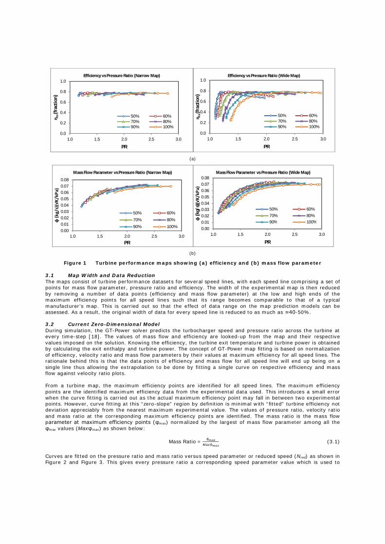
Moraal and Komanovsky (1999) provided an overview of different parameterization methods of turbocharger modelling. A method worth mentioning is the use of artificial neural network for mass flow prediction [3]. Here, the network output which is the mass flow parameter is predicted with speeds, pressure ratios and, if needed, the nozzle vane settings as inputs. The network is trained to associate the output with trained input patterns and subsequently predict the parameter values for given new maps. This method was applied to a compressor and was reported by [11]. The disadvantage of this method is that the training of the input neurons will have to rely heavily on a great quantity of existing data in order to accurately predict new map. With the absence of such data, the model will not offer reliable results. An accurate one-dimensional modelling of turbine performance is described by Romagnoli and Martinez-Botas (2011) for turbines with and without nozzles [12]. This mean line loss model is based on conservation of mass and energy calculations of flow parameters at several stations throughout the turbine assembly. Coefficients of losses are calculated for each station and imposed on the calculated flow parameters. Although the model was validated against experimental data with a broad operating range, no further attempt was made by the authors to extend the mean line map. Nonetheless, these models could serve as a basis for development of a complete turbocharger model for use in one-dimensional gas dynamics engine performance prediction codes. The preceding discussion signifies the importance of turbine map accuracy and range. With regards to the latter aspect, turbocharger experimental facilities which use compressors to balance the turbine power fall short. As acknowledged by [3] and [13], this shortcoming is due to the lack of sensor resolution and sensitivity to capture flow characteristics at low speeds. In addition, discussions thus far have been mainly on steady state maps and methods to predict and extend them. Little information is available in the public domain for methods of modelling unsteady turbine operation. It is a well-known fact that there is a high degree of interaction between the engine and the turbocharger. The former imposes an unsteady, periodic flow onto the turbocharger turbine the flow characteristics of which are, therefore, widely varying and which deviate substantially from the single, optimum, steady-state operating flow condition of the turbine. The maps generated for unsteady turbine operations are not commonly available. Unsteady turbocharger experiments such as those reported in [1] [14], [15] and [16]. Reviews by [17] show that the performance parameters exhibits hysteresis loops around the steady flow points on the maps due to the filling and emptying nature of the flow inside the turbine. It is crucial to point out that the reliability of any map prediction methods is only as good as the experimental data that validates them. In most cases, the range of experimental data is small due to the lack of accurate measuring tools at extreme operating ranges; an issue addressed by [4] and [8]. The majority of models that have been discussed in the preceding section fall short in this aspect. The availability of test facilities which yield a wider data range means that existing methods can be revised and improved if necessary. One-dimensional models require substantial amount of geometrical information, making them less robust for use in simulation software, although having an accurate model as an alternative for users to opt for could be proposed. Classic models such as the adiabatic nozzle are too simplified and cannot realistically represent actual turbine behaviour. Perhaps, a more crucial argument in the context of the present work is that most models are developed and validated against narrow experimental data maps. In cases where the models are purely based on mathematical manipulations of the data, the actual behaviour of the turbine might be misrepresented, consequently affecting the output engine performance calculations. This has been the case with the software used for the presented simulation results. By using a significantly wider, physical efficiency information basis the extrapolation within the software better correlates with the physical reality of flow in the turbine. This serves as a bypass of the fact that the 0D reality of the simulation does not capture the physical reality of the turbine stage expansion process in instances such as where the degree of reaction for example influences the relationship between BSR and efficiency beyond the single-curve representation typical in such simulations. By focusing on the direct correlation between narrow and wide-range turbine experimental data map extrapolation capabilities, this investigation bypasses the requirement for accurate physical representation of the turbocharger turbine itself, which through these 0D models can never be captured fully, anyway; instead the focus is on the effect of extrapolation itself, not on the possible improvement of the representation of the turbine operating characteristic in the overall engine simulation (through, for example, better representation of the degree of reaction or other parameters). 3 MAP PREDICTION METHOD The selection of the turbines in this study depends primarily on the boost requirement for the engine at hand. Two maps obtained from the same turbine are used in this study; one with a wider data range (wide map) and another with several data points removed (narrow map). The original map was obtained tests carried out at the Imperial College turbocharger facility [1]. The efficiency and swallowing capacity (mass flow parameter) of these two maps are shown in Figure 1 below. The map was obtained from a cold flow test at an average inlet total temperature range of 333K to 344K and, therefore, heat transfer effects were not evaluated in this investigation as they were considered to have negligible effect at the temperature range covered. The overall uncertainty for efficiency is ±0.9 – 7.0% with the torque measurement uncertainty at low turbine powers being the main source of error. The uncertainty for mass flow is in the range of 0.87 – 1.9%.

(a)

(b)

Figure 1 Turbine performance maps showing (a) efficiency and (b) mass flow parameter

3.1 Map Width and Data Reduction The maps consist of turbine performance datasets for several speed lines, with each speed line comprising a set of points for mass flow parameter, pressure ratio and efficiency. The width of the experimental map is then reduced by removing a number of data points (efficiency and mass flow parameter) at the low and high ends of the maximum efficiency points for all speed lines such that its range becomes comparable to that of a typical manufacturer’s map. This is carried out so that the effect of data range on the map prediction models can be assessed. As a result, the original width of data for every speed line is reduced to as much as ≈40-50%. 3.2 Current Zero-Dimensional Model During simulation, the GT-Power solver predicts the turbocharger speed and pressure ratio across the turbine at every time-step [18]. The values of mass flow and efficiency are looked-up from the map and their respective values imposed on the solution. Knowing the efficiency, the turbine exit temperature and turbine power is obtained by calculating the exit enthalpy and turbine power. The concept of GT-Power map fitting is based on normalization of efficiency, velocity ratio and mass flow parameters by their values at maximum efficiency for all speed lines. The rationale behind this is that the data points of efficiency and mass flow for all speed line will end up being on a single line thus allowing the extrapolation to be done by fitting a single curve on respective efficiency and mass flow against velocity ratio plots. From a turbine map, the maximum efficiency points are identified for all speed lines. The maximum efficiency points are the identified maximum efficiency data from the experimental data used. This introduces a small error when the curve fitting is carried out as the actual maximum efficiency point may fall in between two experimental points. However, curve fitting at this “zero-slope” region by definition is minimal with “fitted” turbine efficiency not deviation appreciably from the nearest maximum experimental value. The values of pressure ratio, velocity ratio and mass ratio at the corresponding maximum efficiency points are identified. The mass ratio is the mass flow parameter at maximum efficiency points (φmax) normalized by the largest of mass flow parameter among all the φmax values (Maxφmax) as shown below:

Mass Ratio = ∅∅

(3.1)

Curves are fitted on the pressure ratio and mass ratio versus speed parameter or reduced speed (Nred) as shown in Figure 2 and Figure 3. This gives every pressure ratio a corresponding speed parameter value which is used to

0.0

0.2

0.4

0.6

0.8

1.0

1.0 1.5 2.0 2.5 3.0

η ts (

frac

tion)

PR

Efficiency vs Pressure Ratio (Narrow Map)

50% 60%70% 80%90% 100%

0.0

0.2

0.4

0.6

0.8

1.0

1.0 1.5 2.0 2.5 3.0

η ts (

frac

tion)

PR

Efficiency vs Pressure Ratio (Wide Map)

50% 60%70% 80%90% 100%

0.000.010.020.030.040.050.060.070.08

1.0 1.5 2.0 2.5 3.0

φ(k

g/s)

(√K/

kPa)

PR

Mass Flow Parameter vs Pressure Ratio (Narrow Map)

50% 60%70% 80%90% 100% 0.00

0.010.020.030.040.050.060.070.08

1.0 1.5 2.0 2.5 3.0

φ(k

g/s)

(√K/

kPa)

PR

Mass Flow Parameter vs Pressure Ratio (Wide Map)

50% 60%70% 80%90% 100%

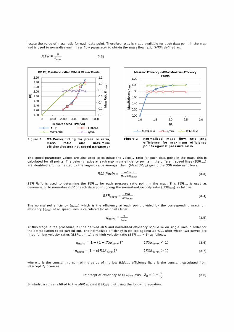
locate the value of mass ratio for each data point. Therefore, φmax is made available for each data point in the map and is used to normalize each mass flow parameter to obtain the mass flow ratio (MFR) defined as:

푀퐹푅 = ∅∅

(3.2)

Figure 2 GT-Power fitting for pressure ratio,

mass ratio and maximum efficiencies against speed parameter

Figure 3 Normalized mass flow rate and

efficiency for maximum efficiency points against pressure ratio

The speed parameter values are also used to calculate the velocity ratio for each data point in the map. This is calculated for all points. The velocity ratios at each maximum efficiency points in the different speed lines (BSRmax) are identified and normalized by the largest value amongst them (MaxBSRmax) giving the BSR Ratio as follows:

퐵푆푅 푅푎푡푖표 = (3.3)

BSR Ratio is used to determine the BSRmax for each pressure ratio point in the map. This BSRmax is used as denominator to normalize BSR of each data point, giving the normalized velocity ratio (BSRnorm) as follows:

퐵푆푅 = (3.4)

The normalized efficiency (ηnorm) which is the efficiency at each point divided by the corresponding maximum efficiency (ηmax) of all speed lines is calculated for all points from:

휂 = (3.5)

At this stage in the procedure, all the derived MFR and normalized efficiency should lie on single lines in order for the extrapolation to be carried out. The normalized efficiency is plotted against BSRnorm after which two curves are fitted for low velocity ratios (BSRnorm < 1) and high velocity ratio (BSRnorm > 1) as follows:

휂 = 1− (1 −퐵푆푅 ) (퐵푆푅 < 1) (3.6)

휂 = 1 − 푐(퐵푆푅 ) (퐵푆푅 ≥ 1) (3.7)

where b is the constant to control the curve of the low BSRnorm efficiency fit, c is the constant calculated from intercept Z0 given as:

Intercept of efficiency at BSRnorm axis, 푍 = 1 +√

(3.8)

Similarly, a curve is fitted to the MFR against BSRnorm plot using the following equation:

0.0

0.2

0.4

0.6

0.8

1.0

1.2

1.001.201.401.601.802.002.202.402.60

0 1000 2000 3000 4000 5000

Mas

s Ra

tio &

ηm

ax

PR

Reduced Speed (RPM/√K)

PR, Eff, MassRatio vs Red RPM at Eff.max Points

PR Fit PR DataMassRatio ηmax

0.00

0.20

0.40

0.60

0.80

1.00

1.20

1.0 1.5 2.0 2.5 3.0

Mas

sRat

io a

nd η

max

PR

Mass and Efficiency vs PR at Maximum Efficiency Points

MassRatio ηmax BSR Ratio

푀퐹푅 = 푐푚 +퐵푆푅 (1− 푐푚) (3.9) where cm is the intercept of the curve at 0.0 BSRnorm and m is an exponent coefficient that controls the curvature of the curve. The values of efficiency and mass flow are extrapolated over the entire range of pressure ratio. The procedure described above is carried out for both the wide and narrow maps prior to the engine simulation. 3.3 Engine Model The engine model that is used in this study is a 4.7 litre direct injection (DI) Diesel engine with some pertinent specifications shown in Table 2. To isolate the effects of turbine maps on the performance of the engine, the engine layout is kept as basic as possible without additional turbine control devices such as wastegates or bypass systems.

Table 2 Basic engine specification

Parameters Specification Combustion System 4-Stroke, V6, Diesel DI Capacity 4.7 litres Compression Ratio 16.5 Bore x Stroke Dimension 100 x 100 mm Induction System Single stage turbocharger

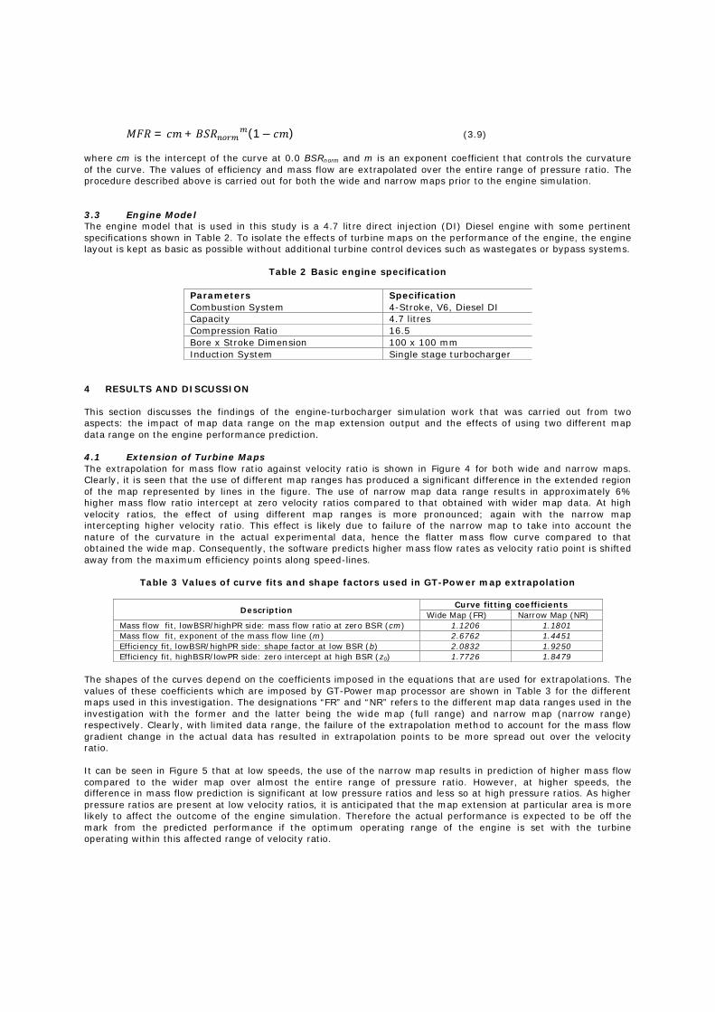
4 RESULTS AND DISCUSSION This section discusses the findings of the engine-turbocharger simulation work that was carried out from two aspects: the impact of map data range on the map extension output and the effects of using two different map data range on the engine performance prediction. 4.1 Extension of Turbine Maps The extrapolation for mass flow ratio against velocity ratio is shown in Figure 4 for both wide and narrow maps. Clearly, it is seen that the use of different map ranges has produced a significant difference in the extended region of the map represented by lines in the figure. The use of narrow map data range results in approximately 6% higher mass flow ratio intercept at zero velocity ratios compared to that obtained with wider map data. At high velocity ratios, the effect of using different map ranges is more pronounced; again with the narrow map intercepting higher velocity ratio. This effect is likely due to failure of the narrow map to take into account the nature of the curvature in the actual experimental data, hence the flatter mass flow curve compared to that obtained the wide map. Consequently, the software predicts higher mass flow rates as velocity ratio point is shifted away from the maximum efficiency points along speed-lines.

Table 3 Values of curve fits and shape factors used in GT-Power map extrapolation

Description Curve fitting coefficients Wide Map (FR) Narrow Map (NR)

Mass flow fit, lowBSR/highPR side: mass flow ratio at zero BSR (cm) 1.1206 1.1801 Mass flow fit, exponent of the mass flow line (m) 2.6762 1.4451 Efficiency fit, lowBSR/highPR side: shape factor at low BSR (b) 2.0832 1.9250 Efficiency fit, highBSR/lowPR side: zero intercept at high BSR (z0) 1.7726 1.8479

The shapes of the curves depend on the coefficients imposed in the equations that are used for extrapolations. The values of these coefficients which are imposed by GT-Power map processor are shown in Table 3 for the different maps used in this investigation. The designations “FR” and “NR” refers to the different map data ranges used in the investigation with the former and the latter being the wide map (full range) and narrow map (narrow range) respectively. Clearly, with limited data range, the failure of the extrapolation method to account for the mass flow gradient change in the actual data has resulted in extrapolation points to be more spread out over the velocity ratio. It can be seen in Figure 5 that at low speeds, the use of the narrow map results in prediction of higher mass flow compared to the wider map over almost the entire range of pressure ratio. However, at higher speeds, the difference in mass flow prediction is significant at low pressure ratios and less so at high pressure ratios. As higher pressure ratios are present at low velocity ratios, it is anticipated that the map extension at particular area is more likely to affect the outcome of the engine simulation. Therefore the actual performance is expected to be off the mark from the predicted performance if the optimum operating range of the engine is set with the turbine operating within this affected range of velocity ratio.

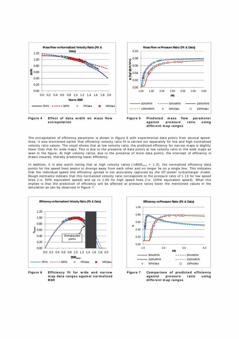
Figure 4 Effect of data width on mass flow extrapolation

Figure 5 Predicted mass flow parameter against pressure ratio using different map ranges

The extrapolation of efficiency parameter is shown in Figure 6 with experimental data points from several speed-lines. It was mentioned earlier that efficiency-velocity ratio fit is carried out separately for low and high normalized velocity ratio values. The result shows that at low velocity ratio, the predicted efficiency for narrow maps is slightly lower than that for wide maps. This is due to the presence of data points at low velocity ratio in the wide maps as seen in the figure. At high velocity ratios, due to the presence of more data points, the intercept of efficiency is drawn inwards, thereby predicting lower efficiency. In addition, it is also worth noting that at high velocity ratios (≈BSRnorm > 1.3), the normalized efficiency data points for the speed lines seems to diverge away from each other and no longer lie on a single line. This indicates that the individual speed line efficiency spread is not accurately captured by the GT-power turbocharger model. Rough estimates indicate that this normalized velocity ratio corresponds to the pressure ratio of 1.13 for low speed lines (i.e. 50% equivalent speed) and up to 1.60 for high speed lines (i.e. 100% equivalent speed). What this implies is that the prediction of efficiency will be affected at pressure ratios lower the mentioned values in the simulation as can be observed in Figure 7.

Figure 6 Efficiency fit for wide and narrow

map data ranges against normalized BSR

Figure 7 Comparison of predicted efficiency

against pressure ratio using different map ranges

0.00

0.20

0.40

0.60

0.80

1.00

1.20

0.0 0.2 0.4 0.6 0.8 1.0 1.2 1.4 1.6 1.8 2.0

MFR

Norm. BSR

Mass Flow vs Normalized Velocity Ratio (Fit & Data)

FR Fit NR Fit FR Data NR Data

0.00

0.02

0.04

0.06

0.08

0.10

1.00 1.50 2.00 2.50 3.00 3.50 4.00

φ(k

g/s)

(√K/

kPa)

PR

Mass Flow vs Pressure Ratio (Fit & Data)

50% FR Fit 50% NR Fit 100% FR Fit

100% NR Fit 50% Data 100% Data

0.00

0.20

0.40

0.60

0.80

1.00

1.20

0.0 0.2 0.4 0.6 0.8 1.0 1.2 1.4 1.6 1.8 2.0

η nor

m

BSRnorm

Efficiency vs Normalized Velocity Ratio (Fit & Data)

FR Fit NR Fit FR Data NR Data

Diverging data points

0.00

0.20

0.40

0.60

0.80

1.00

1.0 2.0 3.0 4.0

η

PR

Efficiency vs Pressure Ratio (Fit & Data)

50% FR Fit 50% NR Fit100% FR Fit 100% NR Fit50% Data 100% Data

4.2 Engine Performance Prediction The engine simulation was carried out for engine speeds ranging from 1000 to 5000 RPM to capture the behaviour of turbine over a wide operating range. Figure 8 shows the basic predicted performance characteristics of the turbocharged engine in terms of brake power and torque whereas Figure 9 shows the volumetric efficiency obtained using the different map ranges. The volumetric efficiency indicates the difference in the breathing capability of the engine. It has to be stated here that due to the unavailability of a directly matching turbocharger turbine map the results of power, volumetric efficiency, BMEP and BSFC start to deviate out of realistic range at the lower half of the engine speed range. The discussion, however, especially as it is based on comparison of methods, stands for some significant trends to be observed, regardless.

Figure 8 Comparison of engine power output and brake torque for simulations using different map data ranges

Figure 9 Comparison of predicted engine volumetric efficiency from using different map data ranges

The brake power and torque are directly related to the engine brake mean effective pressure (BMEP) as shown in Figure 10. BMEP represents the parameter used to compare the engine power regardless of its capacity. It is interesting to note that although the maximum BMEP predicted using both maps are almost the same, the wide map achieves this value at a lower engine speed at approximately 3000 RPM compared to 3500 RPM for the narrow map thus affecting the rating of the engine, although this could be a case of simulation speed point resolution. The use of narrow map resulted in the prediction of lower BMEP with a maximum prediction being 9.8% lower than that for a wider map at 2600RPM.

Figure 10 Predicted engine BMEP for different turbocharger map data range and baseline engine

Figure 11 Comparison of predicted engine BSFC using different map data range

0100200300400500600700

050

100150200250300350400

0 1000 2000 3000 4000 5000 6000

Torq

ue (N

m)

Pow

er (b

hp)

Engine Speed (RPM)

Power Output and Torque vs Engine Speed

T01 FR - Power T01 NR - Power

T01 FR - Torque T01 NR - Torque

0.00.10.20.30.40.50.60.70.80.91.0

0 1000 2000 3000 4000 5000 6000

η vol

Engine Speed (RPM)

Volumetric Efficiency vs Engine Speed

T01 FR - Vol.Eff T01 NR - Vol.Eff

02468

1012141618

0 1000 2000 3000 4000 5000 6000

BMEP

(bar

)

Engine Speed (RPM)

BMEP vs Engine Speed

T01 FR - BMEP T01 NR - BMEP

0

100

200

300

400

500

600

0 1000 2000 3000 4000 5000 6000

BSFC

(g/k

Whr

)

Engine Speed (RPM)

BSFC vs Engine Speed

T01 FR - BSFC T01 NR - BSFC

The increase in volumetric efficiency also affects the fuel consumption of the engine as can be seen in Figure 11. As a result of the increase in brake power in a turbocharged engine, the brake specific fuel consumption, which is the ratio of fuel mass to power, is subsequently reduced when using the wider range map. 4.3 The Effect of Different Map Ranges on Engine Performance Simulation This investigation was set out to analyze the effect of map data range on the engine simulation output. As can be seen in Figure 8 to Figure 11 above, the use of wide and narrow maps indeed affects the predicted engine performance particularly in the region of 2000 to 3000 RPM engine speed despite the fact that the maps used are of the same turbine. For instance, the maximum differences in performance are 9.8% and 10.8% in BMEP and BSFC respectively at 2600 RPM engine speed.

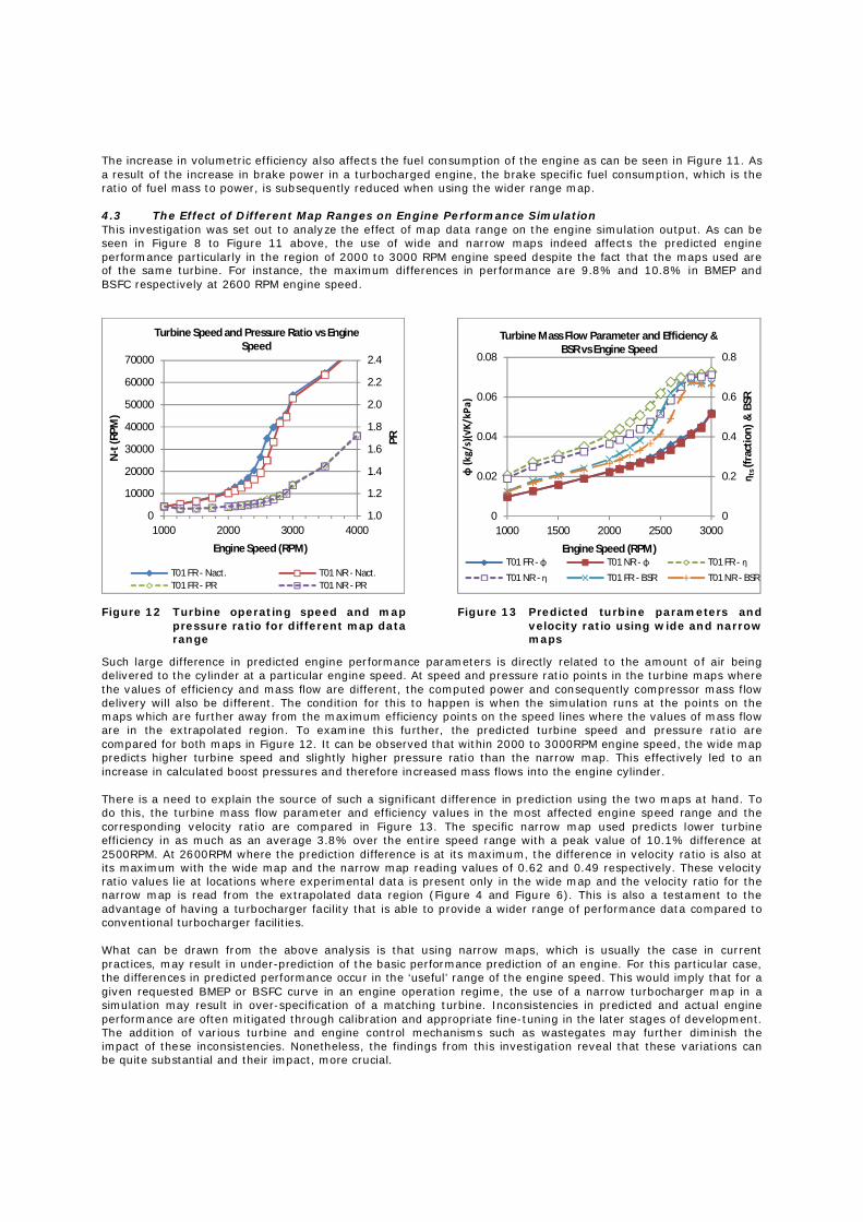
Figure 12 Turbine operating speed and map pressure ratio for different map data range

Figure 13 Predicted turbine parameters and velocity ratio using wide and narrow maps

Such large difference in predicted engine performance parameters is directly related to the amount of air being delivered to the cylinder at a particular engine speed. At speed and pressure ratio points in the turbine maps where the values of efficiency and mass flow are different, the computed power and consequently compressor mass flow delivery will also be different. The condition for this to happen is when the simulation runs at the points on the maps which are further away from the maximum efficiency points on the speed lines where the values of mass flow are in the extrapolated region. To examine this further, the predicted turbine speed and pressure ratio are compared for both maps in Figure 12. It can be observed that within 2000 to 3000RPM engine speed, the wide map predicts higher turbine speed and slightly higher pressure ratio than the narrow map. This effectively led to an increase in calculated boost pressures and therefore increased mass flows into the engine cylinder. There is a need to explain the source of such a significant difference in prediction using the two maps at hand. To do this, the turbine mass flow parameter and efficiency values in the most affected engine speed range and the corresponding velocity ratio are compared in Figure 13. The specific narrow map used predicts lower turbine efficiency in as much as an average 3.8% over the entire speed range with a peak value of 10.1% difference at 2500RPM. At 2600RPM where the prediction difference is at its maximum, the difference in velocity ratio is also at its maximum with the wide map and the narrow map reading values of 0.62 and 0.49 respectively. These velocity ratio values lie at locations where experimental data is present only in the wide map and the velocity ratio for the narrow map is read from the extrapolated data region (Figure 4 and Figure 6). This is also a testament to the advantage of having a turbocharger facility that is able to provide a wider range of performance data compared to conventional turbocharger facilities. What can be drawn from the above analysis is that using narrow maps, which is usually the case in current practices, may result in under-prediction of the basic performance prediction of an engine. For this particular case, the differences in predicted performance occur in the ‘useful’ range of the engine speed. This would imply that for a given requested BMEP or BSFC curve in an engine operation regime, the use of a narrow turbocharger map in a simulation may result in over-specification of a matching turbine. Inconsistencies in predicted and actual engine performance are often mitigated through calibration and appropriate fine-tuning in the later stages of development. The addition of various turbine and engine control mechanisms such as wastegates may further diminish the impact of these inconsistencies. Nonetheless, the findings from this investigation reveal that these variations can be quite substantial and their impact, more crucial.

1.0

1.2

1.4

1.6

1.8

2.0

2.2

2.4

0

10000

20000

30000

40000

50000

60000

70000

1000 2000 3000 4000

PR

N-t

(RPM

)

Engine Speed (RPM)

Turbine Speed and Pressure Ratio vs Engine Speed

T01 FR - Nact. T01 NR - Nact.T01 FR - PR T01 NR - PR

0

0.2

0.4

0.6

0.8

0

0.02

0.04

0.06

0.08

1000 1500 2000 2500 3000

η ts

(frac

tion)

& B

SR

φ(k

g/s)

(√K/

kPa)

Engine Speed (RPM)

Turbine Mass Flow Parameter and Efficiency & BSR vs Engine Speed

T01 FR - φ T01 NR - φ T01 FR - η

T01 NR - η T01 FR - BSR T01 NR - BSR

5 CONCLUSION The map extension procedure in commercial one-dimensional-based engine simulation software, namely GT-Power, has been implemented using maps of a turbine with different data range and the predicted basic engine performance characteristics has been compared for the two maps used. It was found that for this specific simulation, the use of the narrow maps (in the mid velocity ratio range) resulted in prediction of lower BMEP with a maximum prediction being 9.8% lower than that for a wider map. In this particular investigation, the associated brake power and torque are significantly under-predicted especially at mid-range engine speeds (2000 – 3000RPM). The use of narrow maps also results in over-prediction of the engine’s BSFC at the said engine speeds to as much as 10.8% (at 2600RPM). Such substantial inconsistencies will result in larger uncertainties in the later stage of engine calibration and drive cycle evaluation. More inconsistencies in the prediction can be expected when load simulations are carried out. The variation in performance prediction can be traced back to how the range of data affects the extension of the map. Here, GT-Power map processor fails to capture the gradient changes in mass flow and efficiency curves as the GT-Power fitting procedure is carried out. At points which are further away from maximum efficiency points along the speed lines, the performance values for each maps digress away from one another. As a consequence, the difference in the values of turbine mass flow and efficiency looked-up from the predicted maps becomes more apparent, in particular, at low pressure ratios. Although the map extension method employed by GT-Power is robust enough for use in one-dimensional software, in this case, it is the range of data entered into the turbocharger component within the software that has the most profound effect on the outcome of the simulation. This calls for an improved modelling method that is able to represent the complete physical behaviour of a turbine as an alternative to the current methods in a gas dynamics code in the future. The ultimate goal would be to have a model that is able to incorporate steady and unsteady performance parameters of a turbocharger turbine and the same time being compatible with the platform of current engine simulation codes. Nomenclature BMEP = brake mean effective pressure BSFC = brake specific fuel consumption BSR = blade speed ratio (velocity ratio) Cis = isentropic speed cp = specific heat at constant pressure D = diameter FR = wide data range ṁ = mass flow rate MaxBSR = largest value of maximum velocity ratio MFR = mass flow ratio N = rotational speed NR = narrow data range Nred = speed parameter (reduced speed) N-t = turbine actual speed P = pressure PR = pressure ratio R = gas constant T0 = total temperature U = blade tip speed W = turbine work γ = specific heat ratio ηts = total-to-static efficiency ηvol = volumetric efficiency φ = mass flow parameter Subscripts act = actual condition crit = critical condition

in = inlet condition is = isentropic condition max = maximum value norm = normalized value out = exit condition

REFERENCES

[1] S. Szymko, “The Development of an Eddy Current Dynamometer for Evaluation of Steady and Pulsating Turbocharger Turbine Performance,” Imperial College London, 2006.

[2] T. Otobe, P. Grigoriadis, M. Sens, and R. Berndt, “Method of Performance Measurement for Low Turbocharger Speeds,” in 9th International Conference on Turbochargers and Turbocharging, pp. 409-419.

[3] P. Moraal and I. Kolmanovsky, “Turbocharger Modeling for Automotive Control Applications,” SAE Technical Paper Series, no. 1999-01-0908, 1999.

[4] N. Watson and M. S. Janota, Turbocharging the Internal Combustion Engine. London: MacMillan Press, 1982.

[5] J. P. Jensen, A. F. Kristensen, S. C. Sorenson, N. Houbak, and E. Hendricks, “Mean Value Modeling of a Small Turbocharged Diesel Engine,” SAE Technical Paper Series, no. 910070, 1991.

[6] L. Eriksson, “Modeling and Control of Turbocharged SI and DI Engines,” in IFP International Conference, 2007, vol. 62, no. 4, pp. 523-538.

[7] N. C. Baines, “Turbocharger turbine pulse flow performance and modelling – 25 years on,” in 9th International Conference on Turbochargers and Turbocharging, 2010, no. 7, pp. 347-362.

[8] G. Martin, V. Talon, P. Higelin, A. Charlet, and C. Caillol, “Implementing Turbomachinery Physics into Data Map-Based Turbocharger Models,” SAE International Journal of Engines, vol. 2, no. 1, pp. 211-229, 2009.

[9] L. Jiang, J. Vanier, and H. Yilmaz, “Parameterization and Simulation for a Turbocharged Spark Ignition Direct Injection Engine with Variable Valve Timing,” SAE Technical Paper Series, no. 2009-01-0680, 2009.

[10] J. Serrano, F. Arnau, V. Dolz, A. Tiseira, and C. Cervello, “A Model of Turbocharger Radial Turbines Appropriate to be used in Zero- and One-Dimensional Gas Dynamics Codes for Internal Combustion Engines Modelling,” Energy Conversion and Management, vol. 49, pp. 3729-3745, Dec. 2008.

[11] K. Ghorbanian and M. Gholamrezaei, “An Artificial Neural Network Approach to Compressor Performance Prediction,” Applied Energy, vol. 86, no. 7-8, pp. 1210-1221, Jul. 2009.

[12] A. Romagnoli and R. Martinez-Botas, “Performance Prediction of a Nozzled and Nozzleless Mixed-flow Turbine in Steady Conditions,” International Journal of Mechanical Sciences, vol. 53, no. 8, pp. 557-574, Aug. 2011.

[13] M. Jung, R. Ford, K. Glover, N. Collings, U. Christen, and M. J. Watts, “Parameterization and Transient Validation of a Variable Geometry Turbocharger for Mean-value Modeling at Low and Medium Speed-load Points,” SAE Technical Paper Series, no. 2002-01-2729, Citeseer, 2002.

[14] S. Rajoo, “Steady and Pulsating Performance of a Variable Geometry Mixed Flow Turbocharger Turbine,” 2007.

[15] N. Karamanis and R. F. Martinez-Botas, “Mixed-Flow Turbines for Automotive Turbochargers: Steady and Unsteady Performance,” Int. J. Engine Res., vol. 3, no. 3, pp. 127-138, 2002.

[16] C. D. Copeland, R. Martinez-Botas, and M. Seiler, “Comparison Between Steady and Unsteady Double-Entry Turbine Performance Using the Quasi-Steady Assumption,” Journal of Turbomachinery, vol. 133, no. 3, p. 031001, 2011.

[17] S. Rajoo and R. Martinez-Botas, “Mixed Flow Turbine Research: A Review,” Journal of Turbomachinery, vol. 130, no. 4, p. 044001, 2008.

[18] Gamma-Technologies, GT-Suite Flow Theory Manual, V 7.1 ed. 2010.