Rotating Cyclic Systems with Order-Tuned Vibration Absorbers.
University of LiègeFaculty of Applied Sciences
Aerospace and Mechanical Engineering DepartmentStructural Dynamics Research Group
Tuning Methodology of
Nonlinear Vibration Absorbers
Coupled to Nonlinear Mechanical Systems
PhD Thesis Dissertation
by
Viguié Régis
September 2010
Author’s Coordinates
Régis Viguié, Ir.
Structural Dynamics Research GroupAerospace and Mechanical Engineering DepartmentUniversity of LiègeChemin des chevreuils, 14000 LiègeBelgiumOffice phone : + 32 (0)4 366 48 54Email: [email protected]
Rue du Fond d’Or, 3B214300 WaremmeMobile phone : +32 (0)475 21 79 46Email: [email protected]
i
Members of the Examination Committee
Jean-Claude GOLINVAL (President of the committee)Professor - University of LiègeEmail: [email protected]
Gaëtan Kerschen (Thesis Supervisor)Professor - University of LiègeEmail: [email protected]
Olivier BrülsProfessor - University of Liège
Bruno CochelinProfessor - Ecole Centrale de Marseille (Marseille - France)
Vincent DenoëlProfessor - University of Liège
Massimo RuzzeneProfessor - Georgia Institute of Technology (Atlanta - U.S.A.)
Rodolphe SepulchreProfessor - University of Liège
Olivier ThomasProfessor - Conservatoire National des Arts et des Métiers (Paris - France)
ii
Abstract
A large body of literature exists regarding linear and nonlinear dynamic absorbers,but the vast majority of it deals with linear primary structures. However, nonlinearity isa frequency occurrence in engineering applications. Therefore, the present thesis focuseson the mitigation of vibrations of nonlinear primary systems using nonlinear dynamicabsorbers. Because most existing contributions about their design rely on optimizationand sensitivity analysis procedures, which are computationally demanding, or on analyticmethods, which may be limited to small-amplitude motions, this thesis sets the empha-sis on a tuning procedure of nonlinear vibration absorbers that can be computationallytractable and treat strongly nonlinear regimes of motion.
The proposed methodology is a two-step procedure relying on a frequency-energybased approach followed by a bifurcation analysis. The first step, carried out in the freevibration case, imposes the absorber to possess a qualitatively similar dependence onenergy as the primary system. This gives rise to an optimal nonlinear functional formand an initial set of absorber parameters. Based upon these initial results, the secondstep, carried out in the forced vibration case, exploits the relevant information containedwithin the nonlinear frequency response functions, namely, the bifurcation points. Theirtracking in parameter space enables the adjustment of the design parameter values toreach a suitable tuning of the absorber.
The use of the resulting integrated tuning methodology on nonlinear vibration ab-sorbers coupled to systems with nonlinear damping is then investigated. The objectivelies in determining an appropriate functional form for the absorber so that the limit cycleoscillation suppression is maximized.
Finally, the proposed tuning methodology of nonlinear vibration absorbers may im-pose the use of complicated nonlinear functional forms whose practical realization, usingmechanical elements, may be difficult. In this context, an electro-mechanical nonlinearvibration absorber relying on piezoelectric shunting possesses attractive features as vari-ous functional forms for the absorber nonlinearity can be achieved through proper circuitdesign. The foundation of this new approach are laid down and the perspectives arediscussed.
iii

Acknowledgments
I wish to acknowledge the Belgian National Fund for Scientific Research (F.R.I.A.Grant) for its financial support to this research. This disseration is the result of severalyears of research at the University of Liège and I am deeply indebted to a number of peoplewho directly or indirectly helped me pursuing and finishing this doctoral dissertation.
First of all I would like to express my gratitude to my advisor Professeur Gaëtan Ker-schen for the constant help, guidance and encouragement provided during the course ofmy research. I also would like to thank him for giving me so many opportunities of workand life experience with internationally recognized professors in world famous universitiesand conferences.
I also would like to acknowledge Professor Jean-Claude Golinval without whom thestarting of my PhD would not have been possible. I thank him for the confidence he placedin me and the help he brought to me to get the F.R.I.A. grant.
I am pleased to acknowledge my colleagues at the Structural Dynamics Research Groupwho created a pleasant working atmosphere. Particular acknowledgements are given toMaxime Peeters and Fabien Poncelet with whom I had a lot of helpful scientific discus-sions but also and foremost a friendly support.
I have also enjoyed my stays with Professor Massimo Ruzzene at Georgia Instituteof Technology, Professor Erik Johnson at University of Southern California and Dr.Emmanuel Collet at University of Franche-Comté. I am especially grateful to MassimoRuzzene and Erik Johnson for their warm hospitality during my stays in Atlanta and LosAngeles.
I would like to thank Professors Jean-Claude Golinval, Rodolphe Sepulchre, OlivierBrüls, Vincent Denoël, Olivier Thomas, Bruno Cochelin and Massimo Ruzzene for serv-ing on my dissertation examination committee. I am grateful to all of them for acceptingthe heavy task of going through this work.
I am deeply in debt to my parents, grand-parents, brother, sister and family-in-law foralways encouraging me throughout this PhD Thesis.
Finally and foremost, I would like to express my love and gratitude to Dorothée forher infinite patience and understanding and for always being there for me.
iv

In Loving Memory of
My Grandmother, Mamy Odile
My Uncle, Tonton Jean-Marie
v

Contents
1 Introduction 11.1 Vibration Mitigation of Mechanical Structures . . . . . . . . . . . . . . . . 21.2 Linear Vibration Absorbers : The Tuned Mass
Damper . . . . . . . . . . . . . . . . . . . . . . . . . . . . . . . . . . . . . 21.2.1 Linear Single-Degree-of-Freedom Primary Structure . . . . . . . . . 3
1.2.1.1 H∞ Optimization . . . . . . . . . . . . . . . . . . . . . . . 51.2.1.2 H2 Optimization . . . . . . . . . . . . . . . . . . . . . . . 71.2.1.3 Stability Maximization . . . . . . . . . . . . . . . . . . . . 71.2.1.4 Summary of the Optimization Procedures . . . . . . . . . 71.2.1.5 Tuned Mass Damper Performance . . . . . . . . . . . . . 8
1.2.2 Linear Multi-Degree-of-Freedom Primary Structure . . . . . . . . . 111.2.3 Nonlinear Single-Degree-of-Freedom Primary Structure . . . . . . . 11
1.3 Nonlinear Vibration Absorbers . . . . . . . . . . . . . . . . . . . . . . . . . 121.3.1 Pendulum and Impact Vibration Absorbers . . . . . . . . . . . . . 121.3.2 Autoparametric Vibration Absorbers . . . . . . . . . . . . . . . . . 131.3.3 The Nonlinear Energy Sink . . . . . . . . . . . . . . . . . . . . . . 14
1.3.3.1 Linear Single-Degree-of-Freedom Primary Structure . . . . 151.3.3.2 Linear Multi-Degree-of-Freedom Primary Structure . . . . 201.3.3.3 Nonlinear Primary Structure . . . . . . . . . . . . . . . . 23
1.4 Motivation of this Doctoral Dissertation . . . . . . . . . . . . . . . . . . . 251.5 Outline of the Thesis . . . . . . . . . . . . . . . . . . . . . . . . . . . . . . 25
2 Energy Transfer and Dissipation in a Duffing Oscillator Coupled to aNonlinear Attachment 272.1 Introduction . . . . . . . . . . . . . . . . . . . . . . . . . . . . . . . . . . . 282.2 Dynamics of a Duffing Oscillator Coupled to a Nonlinear Energy Sink . . . 28
2.2.1 Nonlinear Energy Sink Performance . . . . . . . . . . . . . . . . . . 282.2.2 Underlying Hamiltonian System . . . . . . . . . . . . . . . . . . . . 322.2.3 Basic Mechanisms for Energy Transfer and Dissipation . . . . . . . 39
2.3 Concluding Remarks . . . . . . . . . . . . . . . . . . . . . . . . . . . . . . 42
3 Tuning Methodology of a Nonlinear Vibration Absorber Coupled to aNonlinear System : Free Vibration 433.1 Introduction . . . . . . . . . . . . . . . . . . . . . . . . . . . . . . . . . . . 44
vi
CONTENTS vii
3.2 Qualitative Tuning Procedure . . . . . . . . . . . . . . . . . . . . . . . . . 443.2.1 Basic Philosophy . . . . . . . . . . . . . . . . . . . . . . . . . . . . 443.2.2 Essentially Nonlinear Primary Structure . . . . . . . . . . . . . . . 45
3.2.2.1 Computation of the Nonlinear Absorber Parameters . . . 453.2.2.2 Results . . . . . . . . . . . . . . . . . . . . . . . . . . . . 473.2.2.3 Further Analysis of the Coupled System . . . . . . . . . . 50
3.2.3 General Nonlinear Primary Structure . . . . . . . . . . . . . . . . . 523.2.3.1 Computation of the Nonlinear Absorber Parameters . . . 523.2.3.2 Results . . . . . . . . . . . . . . . . . . . . . . . . . . . . 533.2.3.3 Further Analysis of the Coupled System . . . . . . . . . . 58
3.3 Quantitative Analysis . . . . . . . . . . . . . . . . . . . . . . . . . . . . . . 593.3.1 Assessment of the Dynamical Absorber Functional Form . . . . . . 59
3.3.1.1 Performance of the Tuned Mass Damper . . . . . . . . . . 593.3.1.2 Performance of the Absorber with Softening Nonlinearity . 673.3.1.3 Performance of the Absorber with Hardening Nonlinearity 67
3.3.2 Determination of the Nonlinear Coefficient kcub . . . . . . . . . . . 673.3.3 Validation of the Results for a Primary Oscillator with Softening
Nonlinearity . . . . . . . . . . . . . . . . . . . . . . . . . . . . . . . 723.4 Concluding Remarks . . . . . . . . . . . . . . . . . . . . . . . . . . . . . . 72
4 Energy-Invariant Nonsimilar Nonlinear Normal Modes in EssentiallyNonlinear Homogeneous Systems 774.1 Introduction . . . . . . . . . . . . . . . . . . . . . . . . . . . . . . . . . . . 784.2 Fundamental Dynamics of an Essentially Nonlinear Two-Degree-of-Freedom
System . . . . . . . . . . . . . . . . . . . . . . . . . . . . . . . . . . . . . . 784.2.1 Linear-Like Dynamics . . . . . . . . . . . . . . . . . . . . . . . . . 794.2.2 Analytical Development . . . . . . . . . . . . . . . . . . . . . . . . 794.2.3 Numerical Approach . . . . . . . . . . . . . . . . . . . . . . . . . . 82
4.2.3.1 Frequency-Energy Plot . . . . . . . . . . . . . . . . . . . . 824.2.3.2 Analysis of the Nonlinear Normal Mode Motions . . . . . 844.2.3.3 Nonlinear Normal Mode Stability . . . . . . . . . . . . . . 87
4.3 Concluding Remarks . . . . . . . . . . . . . . . . . . . . . . . . . . . . . . 87
5 Tuning Methodology of a Nonlinear Vibration Absorber Coupled to aNonlinear System : Forced Vibration 905.1 Introduction . . . . . . . . . . . . . . . . . . . . . . . . . . . . . . . . . . . 915.2 Bifurcation Analysis of an Essentially Nonlinear Two-degree-of-Freedom
System . . . . . . . . . . . . . . . . . . . . . . . . . . . . . . . . . . . . . . 915.2.1 Computation of Nonlinear Frequency Response Functions . . . . . . 915.2.2 Optimization of the Nonlinear Absorber Parameters . . . . . . . . . 95
5.2.2.1 Continuation of Limit Point Bifurcations versus (knl2 ,ω) . 955.2.2.2 Continuation of Limit Point Bifurcations versus (c2,ω) . . 995.2.2.3 Subsequent Iterations . . . . . . . . . . . . . . . . . . . . 995.2.2.4 Other Tuning Conditions . . . . . . . . . . . . . . . . . . 103
CONTENTS viii
5.2.3 Influence of the Forcing Level: Performance-Robustness Analysis . . 1035.3 Extension of the Methodology to Free Response . . . . . . . . . . . . . . . 1065.4 General Nonlinear Primary Structure . . . . . . . . . . . . . . . . . . . . . 1105.5 Concluding Remarks . . . . . . . . . . . . . . . . . . . . . . . . . . . . . . 113
6 Tuning of a Nonlinear Vibration Absorber to Suppress Limit Cycle Os-cillations 1156.1 Introduction . . . . . . . . . . . . . . . . . . . . . . . . . . . . . . . . . . . 1166.2 Drill-String System Dynamics . . . . . . . . . . . . . . . . . . . . . . . . . 1166.3 Suppression of Friction-Induced Limit Cycling by Means of a Nonlinear
Energy Sink : Bifurcation Analysis . . . . . . . . . . . . . . . . . . . . . . 1196.4 Determination of the Functional Form of the Nonlinear Absorber . . . . . 1286.5 Concluding Remarks . . . . . . . . . . . . . . . . . . . . . . . . . . . . . . 128
7 Toward a Practical Realization of a Nonlinear Vibration Absorber 1317.1 Introduction . . . . . . . . . . . . . . . . . . . . . . . . . . . . . . . . . . . 1327.2 Linear Piezoelectric Shunting . . . . . . . . . . . . . . . . . . . . . . . . . 132
7.2.1 Piezoelectric Damping . . . . . . . . . . . . . . . . . . . . . . . . . 1327.2.2 Multimodal and Broadband Damping . . . . . . . . . . . . . . . . . 1337.2.3 Finite Element Formulation . . . . . . . . . . . . . . . . . . . . . . 134
7.3 Nonlinear Piezoelectric Shunting . . . . . . . . . . . . . . . . . . . . . . . . 1357.3.1 Basics . . . . . . . . . . . . . . . . . . . . . . . . . . . . . . . . . . 1357.3.2 Electro-Mechanical System Modeling . . . . . . . . . . . . . . . . . 136
7.4 Qualitative Analysis of a Beam Coupled to a Nonlinear Vibration Absorber 1377.5 Electrical Nonlinear Vibration Absorber Perspectives . . . . . . . . . . . . 140
7.5.1 Short-Term Perspectives . . . . . . . . . . . . . . . . . . . . . . . . 1407.5.1.1 Semi-Experimental Approach . . . . . . . . . . . . . . . . 1407.5.1.2 Essentially Nonlinear Piezoelectric Shunting . . . . . . . . 140
7.5.2 Long-Term Perspectives . . . . . . . . . . . . . . . . . . . . . . . . 1417.6 Concluding Remarks . . . . . . . . . . . . . . . . . . . . . . . . . . . . . . 141
Conclusion 143Directions for Future Work . . . . . . . . . . . . . . . . . . . . . . . . . . . . . . 144
A Solutions of the Tuned Mass Damper Optimization Problems 145A.1 H∞ Optimization . . . . . . . . . . . . . . . . . . . . . . . . . . . . . . . . 145A.2 H2 Optimization . . . . . . . . . . . . . . . . . . . . . . . . . . . . . . . . 146
B Computation of Nonlinear Normal Modes using Numerical Continua-tion 148B.1 Shooting Method . . . . . . . . . . . . . . . . . . . . . . . . . . . . . . . . 148B.2 Continuation of Periodic Solutions . . . . . . . . . . . . . . . . . . . . . . . 149
B.2.1 Predictor step . . . . . . . . . . . . . . . . . . . . . . . . . . . . . . 149B.2.2 Corrector step . . . . . . . . . . . . . . . . . . . . . . . . . . . . . . 150
B.3 NNM Stability . . . . . . . . . . . . . . . . . . . . . . . . . . . . . . . . . 151

ix

CONTENTS x
List of Acronyms
BHA Bottom Hole Assembly
DOF Degree-Of-Freedom
DVA Dynamical Vibration Absorber
FEP Frequency-Energy Plot
FRF Frequency Response Function
LCO Limit Cycle Oscillation
LNM Linear Normal Mode
LO Linear Oscillator
LP Limit Point
LVA Linear Vibration Absorber
MDOF Multi-Degree-Of-Freedom
NES Nonlinear Energy Sink
NLFRF Nonlinear Frequency Response Function
NLVA Nonlinear Vibration Absorber
NNM Nonlinear Normal Mode
NS Neimarck-Sacker
PD Period Doubling
RCC Resonance Cascade Capture
SDOF Single-Degree-Of-Freedom
TET Targeted Energy Transfer
TRC Transient Resonance Capture
TMD Tuned Mass Damper
WT Wavelet Transform
Chapter 1
Introduction
Abstract
This introductory chapter focuses on the necessity of mitigating the vibrationsof mechanical structures targeting better reliability and longer lifespan. Thedifferent classes of vibration mitigation devices are briefly discussed amongwhich the case of passive vibration mitigation is investigated in greater detail.In particular, a review of linear and nonlinear dynamical absorbers is carriedout. The properties, drawbacks and advantages of each absorber type arehighlighted. A particular emphasis is set upon the lack of amplitude robustnessassociated with nonlinear absorbers. Finally, the objectives and the outline ofthe thesis are presented.
1
Chapter 1. Introduction 2
1.1 Vibration Mitigation of Mechanical Structures
Throughout their life, engineering structures undergo multiple sources of vibrations.The control of these vibrations in mechanical systems is still a flourishing research fieldas it enables resistance improvement as well as noise reduction and thereby comfort en-hancement. Vibration reduction methods are classified into three distinct categories :
1. active control has been widely developed throughout the last fifteen years, despitethe simplicity of the underlying principle [1]. Schematically, the goal lies in reducingan undesirable perturbation by generating an out-of-phase motion so that destruc-tive interferences are generated. Active control generally gives the best vibrationreduction performance, but it is not widely used due to its related cost, the necessityto have an external energy supply and its lack of robustness and reliability in anindustrial environment.
2. semi-active control of flexible structures using electro- and magneto-rheological flu-ids was recently proposed [2,3]. The particularity of these fluids lies in their varyingviscosity with respect to the electric or magnetic field in which they are plunged.Since no energy is transferred to the controlled system, these techniques are robustand reliable while offering a vibration reduction level similar to active techniques.However, the modeling of the fluid behaviors as well as the development of the con-troller represent major challenges that still complicate the use of the systems forreal-life structures.
3. passive vibration mitigation methods imply a structural modification by adding ei-ther a dissipative material (e.g., viscoelastic material [4]) or a dynamical vibrationabsorber (DVA) [5, 6]. They represent a very interesting alternative to the afore-mentioned methods as their performance is acceptable without requiring externalenergy supply.
Because this thesis focuses on passive vibration mitigation, a detailed description oflinear and nonlinear DVAs is carried out in the coming sections.
1.2 Linear Vibration Absorbers : The Tuned Mass
Damper
The tuned mass damper (TMD) is probably the most popular device for passive vi-bration mitigation of mechanical structures. It is commonly used for civil (e.g., Milleniumbridge, Taipei 101 and Burj-el-Arab buildings) and electromechanical engineering struc-tures (e.g., cars and high-tension lines). Its broad range of applications is mainly dueto its linear character and thereby the solid theoretical and mathematical foundationson which it relies. Despite the well-established theory for simple primary systems, thedesign of such an absorber is still a challenging problem when it is coupled to morecomplex structures. The present section aims to review the existing tuning procedures
Chapter 1. Introduction 3
k1 k2
m1 m2
x1
F cos ωt
x2
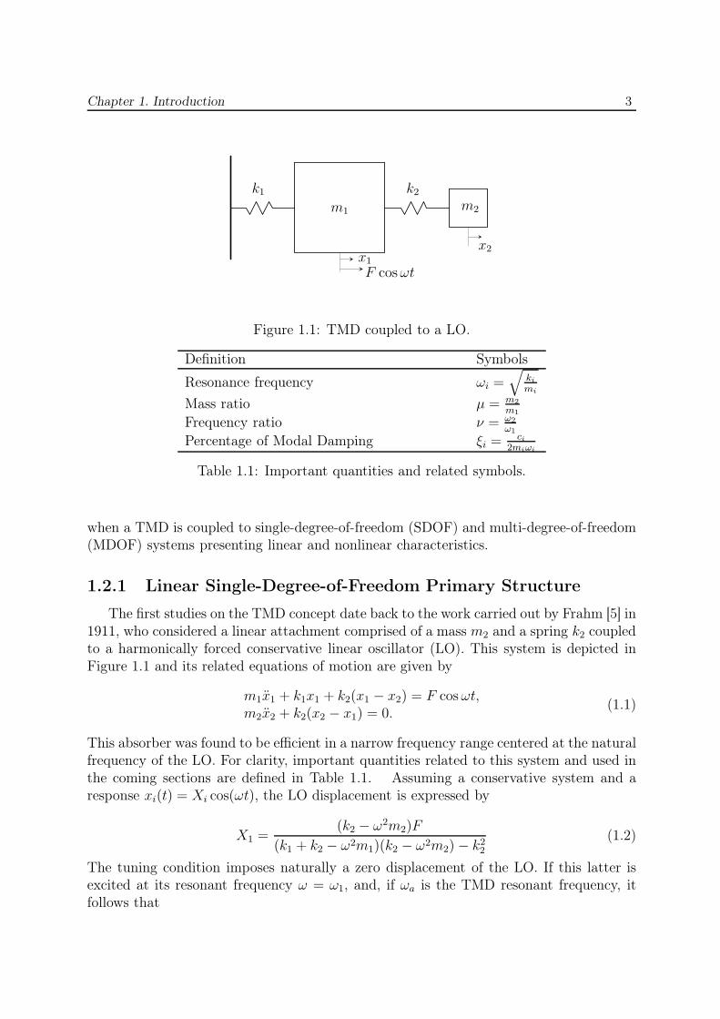
Figure 1.1: TMD coupled to a LO.
Definition Symbols
Resonance frequency ωi =√
ki
mi
Mass ratio µ = m2
m1
Frequency ratio ν = ω2
ω1
Percentage of Modal Damping ξi = ci
2miωi
Table 1.1: Important quantities and related symbols.
when a TMD is coupled to single-degree-of-freedom (SDOF) and multi-degree-of-freedom(MDOF) systems presenting linear and nonlinear characteristics.
1.2.1 Linear Single-Degree-of-Freedom Primary Structure
The first studies on the TMD concept date back to the work carried out by Frahm [5] in1911, who considered a linear attachment comprised of a mass m2 and a spring k2 coupledto a harmonically forced conservative linear oscillator (LO). This system is depicted inFigure 1.1 and its related equations of motion are given by
m1x1 + k1x1 + k2(x1 − x2) = F cos ωt,m2x2 + k2(x2 − x1) = 0.
(1.1)
This absorber was found to be efficient in a narrow frequency range centered at the naturalfrequency of the LO. For clarity, important quantities related to this system and used inthe coming sections are defined in Table 1.1. Assuming a conservative system and aresponse xi(t) = Xi cos(ωt), the LO displacement is expressed by
X1 =(k2 − ω2m2)F
(k1 + k2 − ω2m1)(k2 − ω2m2) − k22
(1.2)
The tuning condition imposes naturally a zero displacement of the LO. If this latter isexcited at its resonant frequency ω = ω1, and, if ωa is the TMD resonant frequency, itfollows that
Chapter 1. Introduction 4
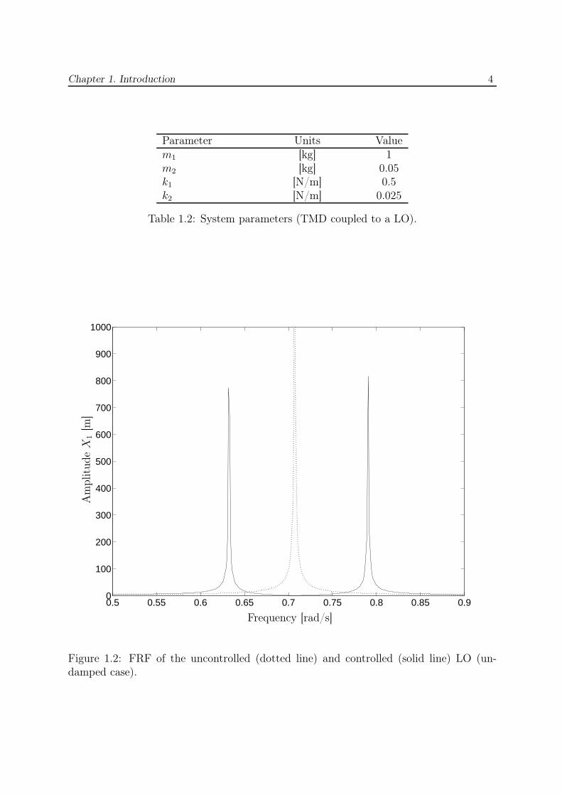
Parameter Units Valuem1 [kg] 1m2 [kg] 0.05k1 [N/m] 0.5k2 [N/m] 0.025
Table 1.2: System parameters (TMD coupled to a LO).
0.5 0.55 0.6 0.65 0.7 0.75 0.8 0.85 0.90
100
200
300
400
500
600
700
800
900
1000
Frequency [rad/s]
Am
plitu
de
X1
[m]
Figure 1.2: FRF of the uncontrolled (dotted line) and controlled (solid line) LO (un-damped case).
Chapter 1. Introduction 5
ωa =
√
k2
m2
=
√
k1
m1
= ω1 (1.3)
This formula is the key relation associated with the tuning of a TMD coupled to a LO.Using the parameter values in Table 1.2, the absorber efficiency can be assessed throughthe computation of the frequency response functions (FRFs) depicted in Figure 1.2. Thesolid line shows the isolation of the primary structure (x1 = 0) at its resonant frequency(ω = 0.707 [rad/s]). However, this tuning condition presents frequency robustness limi-tations. Indeed, the coupled system possesses two resonance peaks in the direct neighbor-hood (ω = 0.63 and = 0.79 [rad/s]) of the antiresonance frequency (ωa = 0.707 [rad/s]).This implies the occurrence of large displacements for slightly varying natural frequencies(i.e., mistuning phenomenon).
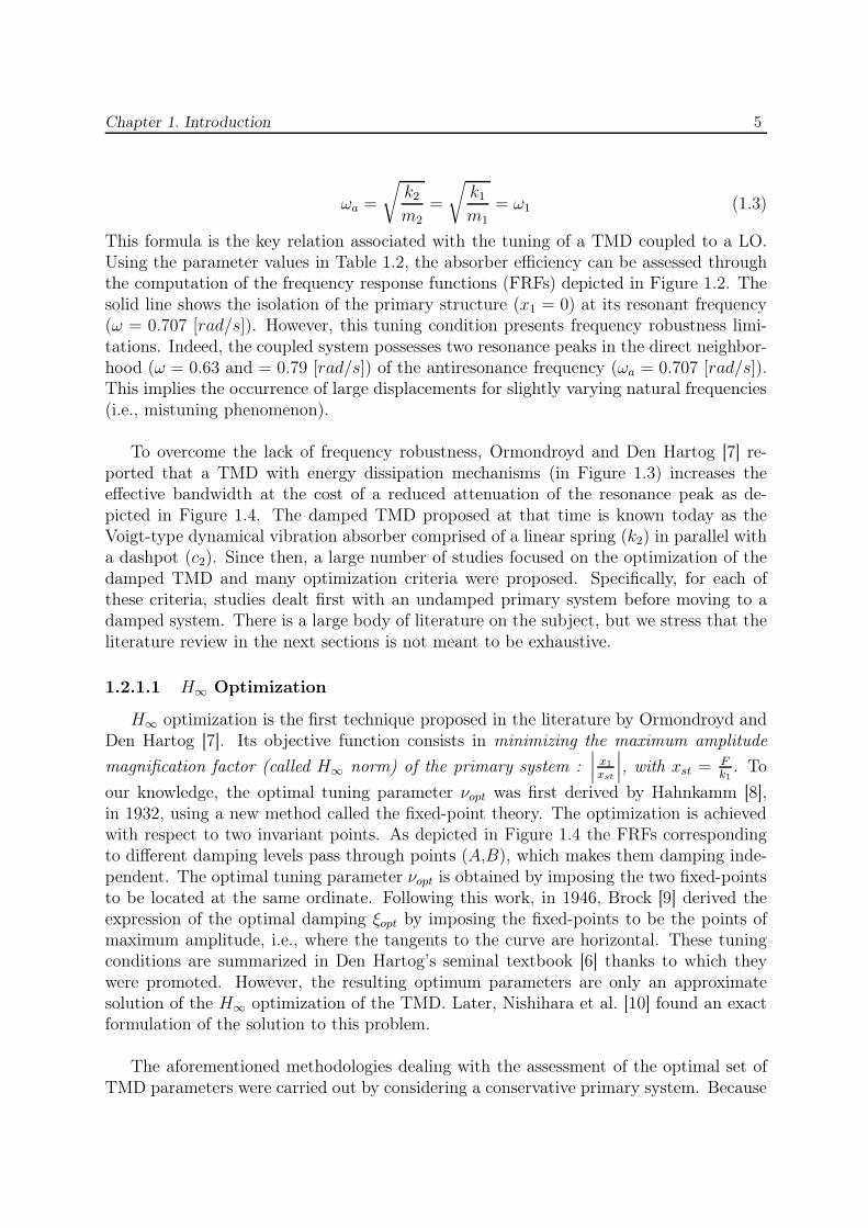
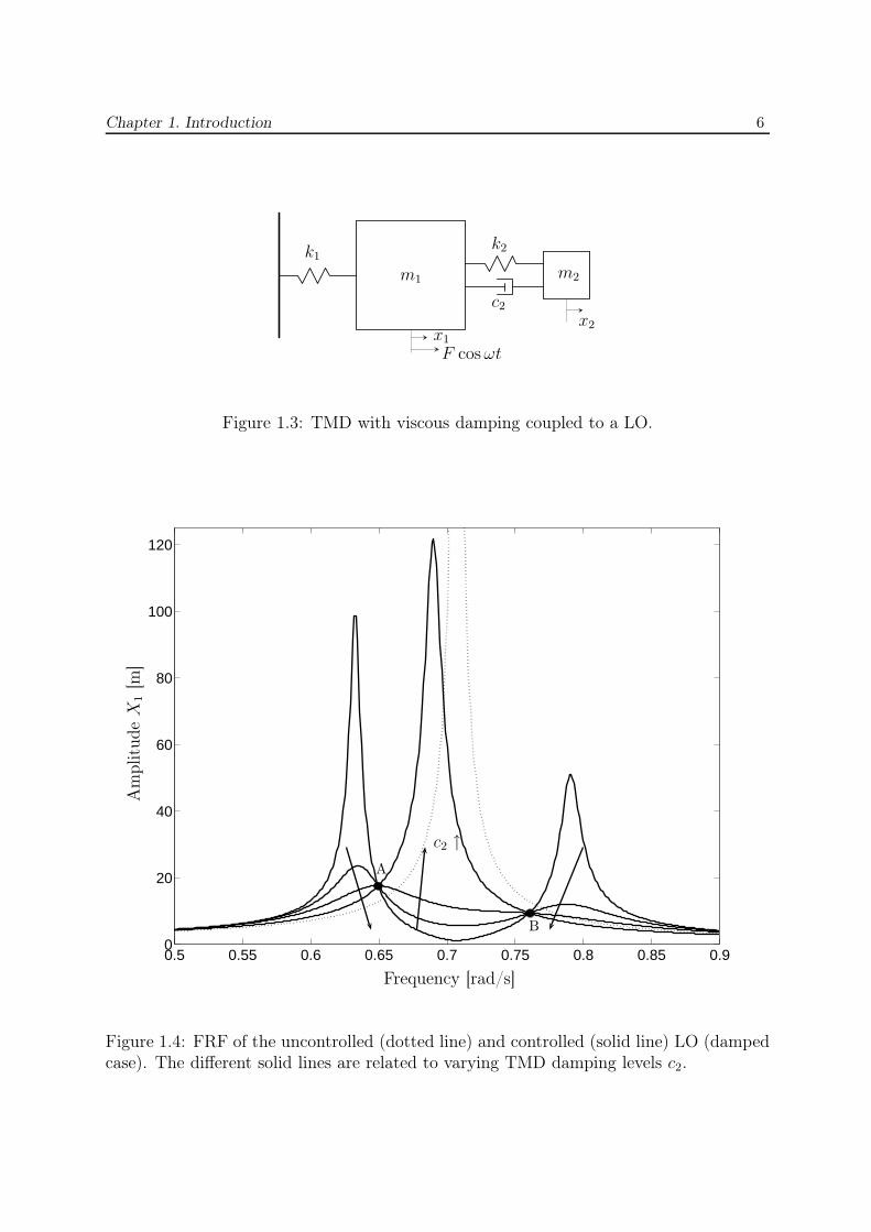
To overcome the lack of frequency robustness, Ormondroyd and Den Hartog [7] re-ported that a TMD with energy dissipation mechanisms (in Figure 1.3) increases theeffective bandwidth at the cost of a reduced attenuation of the resonance peak as de-picted in Figure 1.4. The damped TMD proposed at that time is known today as theVoigt-type dynamical vibration absorber comprised of a linear spring (k2) in parallel witha dashpot (c2). Since then, a large number of studies focused on the optimization of thedamped TMD and many optimization criteria were proposed. Specifically, for each ofthese criteria, studies dealt first with an undamped primary system before moving to adamped system. There is a large body of literature on the subject, but we stress that theliterature review in the next sections is not meant to be exhaustive.
1.2.1.1 H∞ Optimization
H∞ optimization is the first technique proposed in the literature by Ormondroyd andDen Hartog [7]. Its objective function consists in minimizing the maximum amplitude
magnification factor (called H∞ norm) of the primary system :∣
∣
∣
x1
xst
∣
∣
∣, with xst = F
k1. To
our knowledge, the optimal tuning parameter νopt was first derived by Hahnkamm [8],in 1932, using a new method called the fixed-point theory. The optimization is achievedwith respect to two invariant points. As depicted in Figure 1.4 the FRFs correspondingto different damping levels pass through points (A,B), which makes them damping inde-pendent. The optimal tuning parameter νopt is obtained by imposing the two fixed-pointsto be located at the same ordinate. Following this work, in 1946, Brock [9] derived theexpression of the optimal damping ξopt by imposing the fixed-points to be the points ofmaximum amplitude, i.e., where the tangents to the curve are horizontal. These tuningconditions are summarized in Den Hartog’s seminal textbook [6] thanks to which theywere promoted. However, the resulting optimum parameters are only an approximatesolution of the H∞ optimization of the TMD. Later, Nishihara et al. [10] found an exactformulation of the solution to this problem.
The aforementioned methodologies dealing with the assessment of the optimal set ofTMD parameters were carried out by considering a conservative primary system. Because
Chapter 1. Introduction 6
k1k2
c2
m1 m2
x1
F cos ωt
x2
Figure 1.3: TMD with viscous damping coupled to a LO.
0.5 0.55 0.6 0.65 0.7 0.75 0.8 0.85 0.90
20
40
60
80
100
120
B
A
Frequency [rad/s]
Am
plitu
de
X1
[m]
c2 ↑
Figure 1.4: FRF of the uncontrolled (dotted line) and controlled (solid line) LO (dampedcase). The different solid lines are related to varying TMD damping levels c2.
Chapter 1. Introduction 7
this assumption is too restrictive, damping is to be introduced into the primary structure,and H∞ optimization of the TMD is reconsidered. In this context, the fixed-point theoryis no longer available, because the invariant points do not exist anymore. Surprisingly, aclosed-from solution cannot be worked out even though a seemingly simple 2DOF linearsystem is studied. Therefore, many studies focused on the assessment of the optimalabsorber parameters when the primary system has significant damping. Pennestri [11]applied Chebyshev’s min-max criterion, whereas Thompson [12, 13] tackled the problemfrom a control perspective using a frequency locus approach to minimize the systemresponses. Other works focused on the derivation of series solutions using perturbationmethods [14–16]. As an example of the related complex formulation, these solutions aregiven in Appendix A. Finally, most of the efforts were devoted to numerical approachesassociated with the optimization of performance variables or nonlinear programming [13,16–21].
1.2.1.2 H2 Optimization
If the primary system is subjected to broadband random excitation, it is not of inter-est to consider only the resonant frequency of the system. Indeed, a slight mistuning ofthis latter would modify the resonant frequency to another locus and render the TMDinefficient. Therefore, an optimization criterion is to be developed so that the frequencyrobustness associated with acceptable performance is ensured. The so-called H2 opti-mization of DVAs was proposed by Crandall and Mark [22] in 1963. The underlyingobjective is to reduce the total vibration energy of the system over all frequencies. In thisoptimization criterion, the area (called H2 norm) under the frequency response curve ofthe system is minimized. The exact solution for the DVA attached to undamped primarysystems was derived by Iwata [19] and Asami [14]. In the general case including damping,numerical, series and exact algebraic solutions detailed in Appendix A were introducedby Asami in [14], [23] and [15], respectively.
1.2.1.3 Stability Maximization
The objective of H∞ and H2 optimizations is to improve the steady-state response ofthe primary system. On the other hand, the objective of stability maximization lies in theimprovement of the transient vibration of the system. This criterion was first proposedby Yamagushi [24] in 1988. Additional developments were carried out by Nishihara etal. [25], who found that the method was fulfilled when the poles of the system transferfunction are located as far as possible from the imaginary axis in the left-hand plane.Exact solutions are available for both undamped and damped cases.
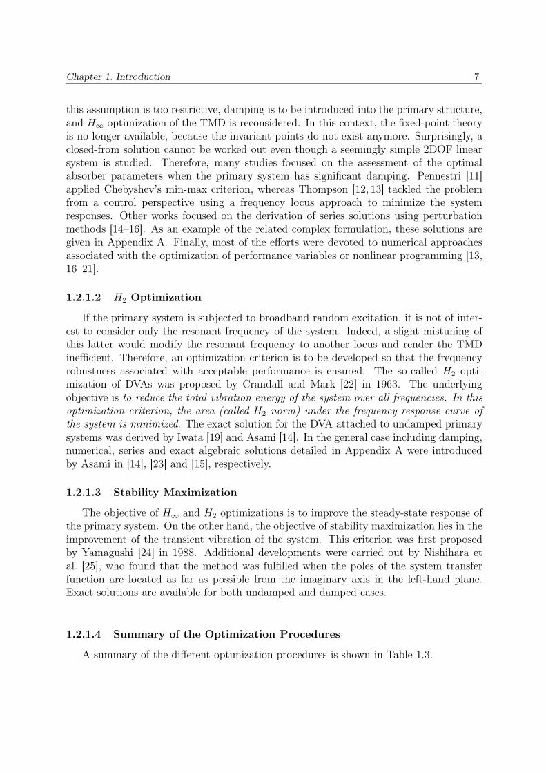
1.2.1.4 Summary of the Optimization Procedures
A summary of the different optimization procedures is shown in Table 1.3.
Chapter 1. Introduction 8
Optimi-
zation
Undamped primary system Damped primary systemApproximation Exact Numerical Series Exact
H∞
Frahm [5]Den Hartog [6, 7]Hahnkamm [8]Brock [9]
Nishihara [25]
Ikeda [26]Randall [27]Thomson[12, 13]Jordanov [20,21]Soom [28]Sekiguchi [17]
Asami [15]
Fujino [16]
Probably
Impossible
H2 /Iwata [19]
Asami [14]Asami [14] Asami [23] Asami [15]
Stabi-lity
/Yamaguchi [24]
Nishihara [25]/ /
Nishihara
[25]
Table 1.3: Summary of the DVA optimization.
1.2.1.5 Tuned Mass Damper Performance
Considering the basic tuning condition, expressed in Equation (1.3), and assumingthat weak damping (c1 = c2 = 0.002 [Ns/m]) is introduced in both oscillators so thatenergy dissipation can be induced, the TMD performance is examined. The resultingsystem is governed by the following equations of motion :
m1x1 + c1x1 + c2(x1 − x2) + k1x1 + k2(x1 − x2) = F cos ωt,m2x2 + c2(x2 − x1) + k2(x2 − x1) = 0.
(1.4)
whose parameter values are listed in Table 1.2, and direct impulsive forcing of the LO isachieved by imparting a non-zero initial velocity to the LO (x1(0) 6= 0, x1(0) = x2(0) =x2(0) = 0). The performance of the absorber is computed using numerical integrationand assessed using the ratio between the energy dissipated in the TMD and the inputenergy :
Ediss,absorber,%(t) = 100
c2
t∫
0
(x1(τ) − x2(τ))2dτ
12m1x1(0)2
(1.5)
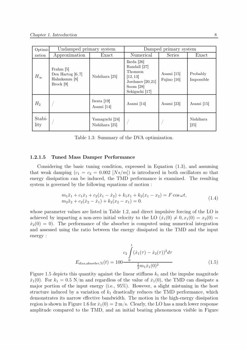
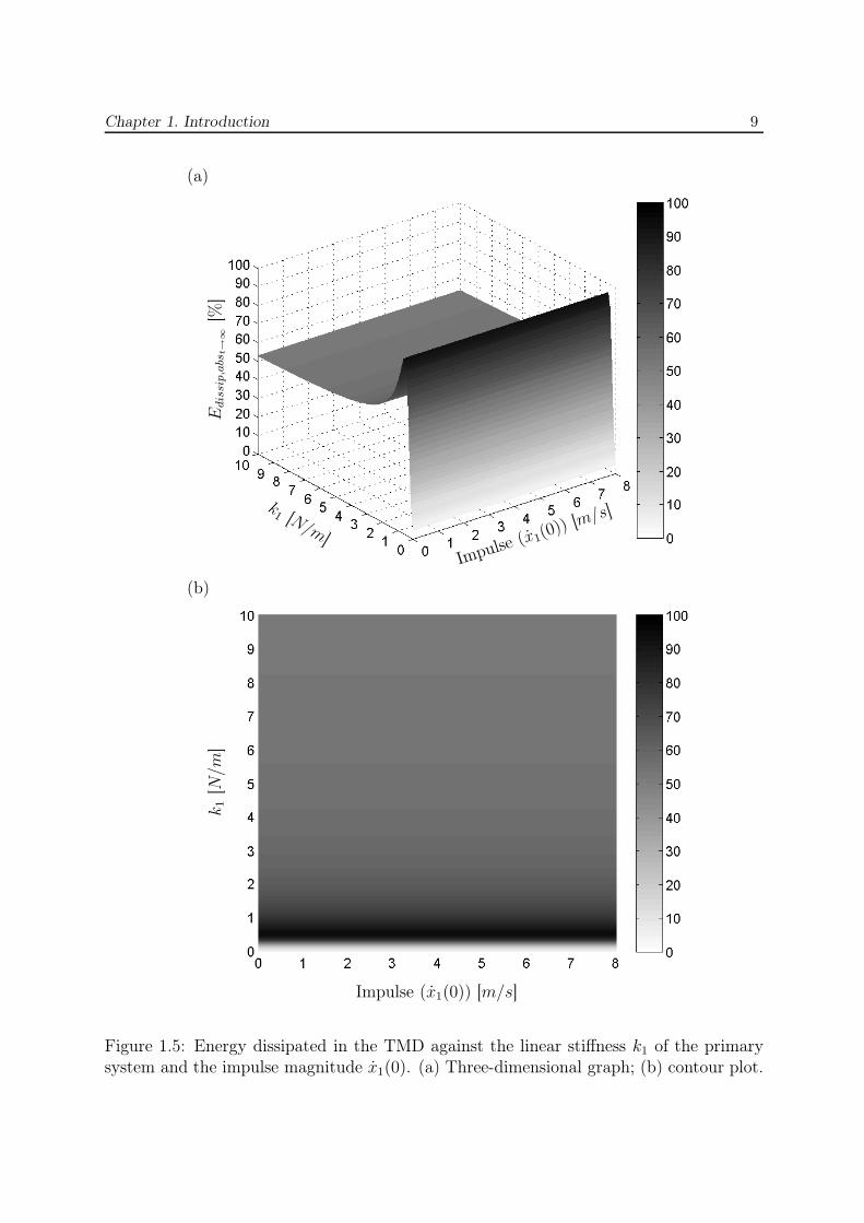
Figure 1.5 depicts this quantity against the linear stiffness k1 and the impulse magnitudex1(0). For k1 = 0.5 N/m and regardless of the value of x1(0), the TMD can dissipate amajor portion of the input energy (i.e., 95%). However, a slight mistuning in the hoststructure induced by a variation of k1 drastically reduces the TMD performance, whichdemonstrates its narrow effective bandwidth. The motion in the high-energy dissipationregion is shown in Figure 1.6 for x1(0) = 2 m/s. Clearly, the LO has a much lower responseamplitude compared to the TMD, and an initial beating phenomenon visible in Figure
Chapter 1. Introduction 9
Impulse (x1(0)) [m/s]
k1 [N/m]
Edis
sip,a
bst→
∞[%
]
(a)
Impulse (x1(0)) [m/s]
k1
[N/m
]
(b)
Figure 1.5: Energy dissipated in the TMD against the linear stiffness k1 of the primarysystem and the impulse magnitude x1(0). (a) Three-dimensional graph; (b) contour plot.
Chapter 1. Introduction 10
0 100 200 300 400 500 600 700 800 900 1000−8
−6
−4
−2
0
2
4
6
8
Time [s]
Am
plitu
de
[m]
(a)
0 50 100 150 200 250 300−8
−6
−4
−2
0
2
4
6
8
Time [s]
Am
plitu
de
[m]
(b)
0 100 200 300 400 500 600 700 800 900 10000
10
20
30
40
50
60
70
80
90
100
Time [s]
Inst
anta
neo
us
Ener
gy
[%]
(c)
0 100 200 300 400 500 600 700 800 900 10000
10
20
30
40
50
60
70
80
90
100
Time [s]
Tota
lD
iss
Ener
gy
[%]
(d)
Figure 1.6: Dynamics of a TMD coupled to a LO. The dotted and solid lines correspondto the TMD and LO, respectively. (a) Displacement responses; (b) close-up for early-timeresponse; (c) percentage of instantaneous total energy in both oscillators; (d) percentageof total energy dissipated in the absorber.
Chapter 1. Introduction 11
1.6(b) is followed by a 1 : 1 in-phase motion of the two masses. Looking at Figure 1.6(d)reveals the importance of the beating regime in the TMD performance. Strong energyexchanges occur between both oscillators and allow most of the energy initially impartedto the LO to be dissipated into the absorber.
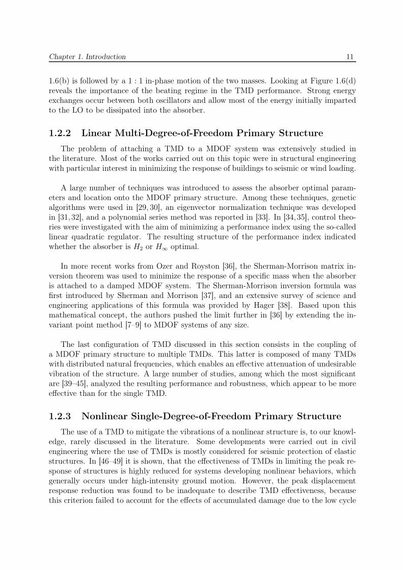
1.2.2 Linear Multi-Degree-of-Freedom Primary Structure
The problem of attaching a TMD to a MDOF system was extensively studied inthe literature. Most of the works carried out on this topic were in structural engineeringwith particular interest in minimizing the response of buildings to seismic or wind loading.
A large number of techniques was introduced to assess the absorber optimal param-eters and location onto the MDOF primary structure. Among these techniques, geneticalgorithms were used in [29, 30], an eigenvector normalization technique was developedin [31,32], and a polynomial series method was reported in [33]. In [34,35], control theo-ries were investigated with the aim of minimizing a performance index using the so-calledlinear quadratic regulator. The resulting structure of the performance index indicatedwhether the absorber is H2 or H∞ optimal.
In more recent works from Ozer and Royston [36], the Sherman-Morrison matrix in-version theorem was used to minimize the response of a specific mass when the absorberis attached to a damped MDOF system. The Sherman-Morrison inversion formula wasfirst introduced by Sherman and Morrison [37], and an extensive survey of science andengineering applications of this formula was provided by Hager [38]. Based upon thismathematical concept, the authors pushed the limit further in [36] by extending the in-variant point method [7–9] to MDOF systems of any size.
The last configuration of TMD discussed in this section consists in the coupling ofa MDOF primary structure to multiple TMDs. This latter is composed of many TMDswith distributed natural frequencies, which enables an effective attenuation of undesirablevibration of the structure. A large number of studies, among which the most significantare [39–45], analyzed the resulting performance and robustness, which appear to be moreeffective than for the single TMD.
1.2.3 Nonlinear Single-Degree-of-Freedom Primary Structure
The use of a TMD to mitigate the vibrations of a nonlinear structure is, to our knowl-edge, rarely discussed in the literature. Some developments were carried out in civilengineering where the use of TMDs is mostly considered for seismic protection of elasticstructures. In [46–49] it is shown, that the effectiveness of TMDs in limiting the peak re-sponse of structures is highly reduced for systems developing nonlinear behaviors, whichgenerally occurs under high-intensity ground motion. However, the peak displacementresponse reduction was found to be inadequate to describe TMD effectiveness, becausethis criterion failed to account for the effects of accumulated damage due to the low cycle
Chapter 1. Introduction 12
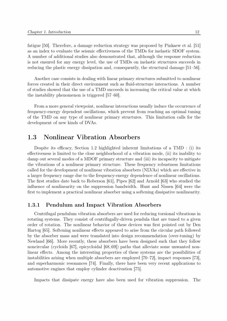
fatigue [50]. Therefore, a damage reduction strategy was proposed by Pinkaew et al. [51]as an index to evaluate the seismic effectiveness of the TMDs for inelastic SDOF system.A number of additional studies also demonstrated that, although the response reductionis not ensured for any energy level, the use of TMDs on inelastic structures succeeds inreducing the plastic energy dissipation and, consequently, the structural damage [51–56].
Another case consists in dealing with linear primary structures submitted to nonlinearforces created in their direct environment such as fluid-structure interactions. A numberof studies showed that the use of a TMD succeeds in increasing the critical value at whichthe instability phenomenon is triggered [57–60].
From a more general viewpoint, nonlinear interactions usually induce the occurrence offrequency-energy dependent oscillations, which prevent from reaching an optimal tuningof the TMD on any type of nonlinear primary structures. This limitation calls for thedevelopment of new kinds of DVAs.
1.3 Nonlinear Vibration Absorbers
Despite its efficacy, Section 1.2 highlighted inherent limitations of a TMD : (i) itseffectiveness is limited to the close neighborhood of a vibration mode, (ii) its inability todamp out several modes of a MDOF primary structure and (iii) its incapacity to mitigatethe vibrations of a nonlinear primary structure. These frequency robustness limitationscalled for the development of nonlinear vibration absorbers (NLVAs) which are effective ina larger frequency range due to the frequency-energy dependence of nonlinear oscillations.The first studies date back to Roberson [61], Pipes [62] and Arnold [63] who studied theinfluence of nonlinearity on the suppression bandwidth. Hunt and Nissen [64] were thefirst to implement a practical nonlinear absorber using a softening dissipative nonlinearity.
1.3.1 Pendulum and Impact Vibration Absorbers
Centrifugal pendulum vibration absorbers are used for reducing torsional vibrations inrotating systems. They consist of centrifugally-driven pendula that are tuned to a givenorder of rotation. The nonlinear behavior of these devices was first pointed out by DenHartog [65]. Softening nonlinear effects appeared to arise from the circular path followedby the absorber mass and were translated into design recommendation (over-tuning) byNewland [66]. More recently, these absorbers have been designed such that they follownoncircular (cycloids [67], epicycloidal [68, 69]) paths that alleviate some unwanted non-linear effects. Among the interesting properties of these systems are the possibilities ofinstabilities arising when multiple absorbers are employed [70–72], impact responses [73],and superharmonic resonances [74]. Finally, there have been very recent applications toautomotive engines that employ cylinder deactivation [75].
Impacts that dissipate energy have also been used for vibration suppression. The
Chapter 1. Introduction 13
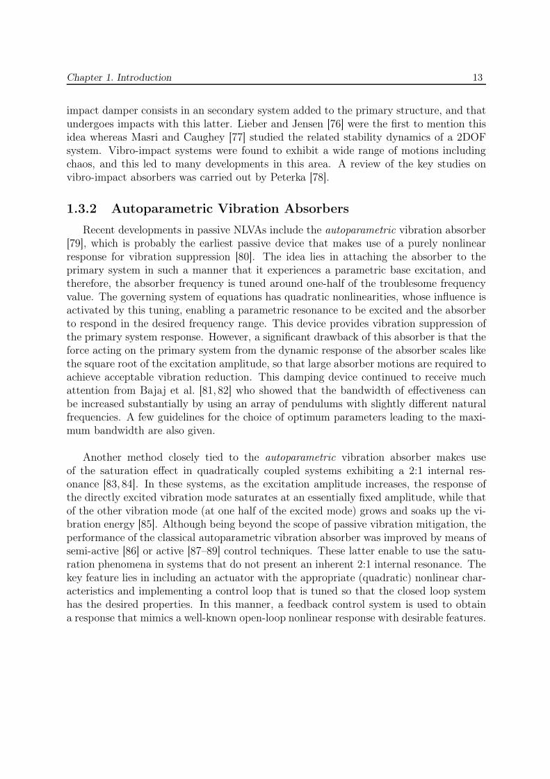
impact damper consists in an secondary system added to the primary structure, and thatundergoes impacts with this latter. Lieber and Jensen [76] were the first to mention thisidea whereas Masri and Caughey [77] studied the related stability dynamics of a 2DOFsystem. Vibro-impact systems were found to exhibit a wide range of motions includingchaos, and this led to many developments in this area. A review of the key studies onvibro-impact absorbers was carried out by Peterka [78].
1.3.2 Autoparametric Vibration Absorbers
Recent developments in passive NLVAs include the autoparametric vibration absorber[79], which is probably the earliest passive device that makes use of a purely nonlinearresponse for vibration suppression [80]. The idea lies in attaching the absorber to theprimary system in such a manner that it experiences a parametric base excitation, andtherefore, the absorber frequency is tuned around one-half of the troublesome frequencyvalue. The governing system of equations has quadratic nonlinearities, whose influence isactivated by this tuning, enabling a parametric resonance to be excited and the absorberto respond in the desired frequency range. This device provides vibration suppression ofthe primary system response. However, a significant drawback of this absorber is that theforce acting on the primary system from the dynamic response of the absorber scales likethe square root of the excitation amplitude, so that large absorber motions are required toachieve acceptable vibration reduction. This damping device continued to receive muchattention from Bajaj et al. [81, 82] who showed that the bandwidth of effectiveness canbe increased substantially by using an array of pendulums with slightly different naturalfrequencies. A few guidelines for the choice of optimum parameters leading to the maxi-mum bandwidth are also given.
Another method closely tied to the autoparametric vibration absorber makes useof the saturation effect in quadratically coupled systems exhibiting a 2:1 internal res-onance [83, 84]. In these systems, as the excitation amplitude increases, the response ofthe directly excited vibration mode saturates at an essentially fixed amplitude, while thatof the other vibration mode (at one half of the excited mode) grows and soaks up the vi-bration energy [85]. Although being beyond the scope of passive vibration mitigation, theperformance of the classical autoparametric vibration absorber was improved by means ofsemi-active [86] or active [87–89] control techniques. These latter enable to use the satu-ration phenomena in systems that do not present an inherent 2:1 internal resonance. Thekey feature lies in including an actuator with the appropriate (quadratic) nonlinear char-acteristics and implementing a control loop that is tuned so that the closed loop systemhas the desired properties. In this manner, a feedback control system is used to obtaina response that mimics a well-known open-loop nonlinear response with desirable features.
Chapter 1. Introduction 14
1.3.3 The Nonlinear Energy Sink
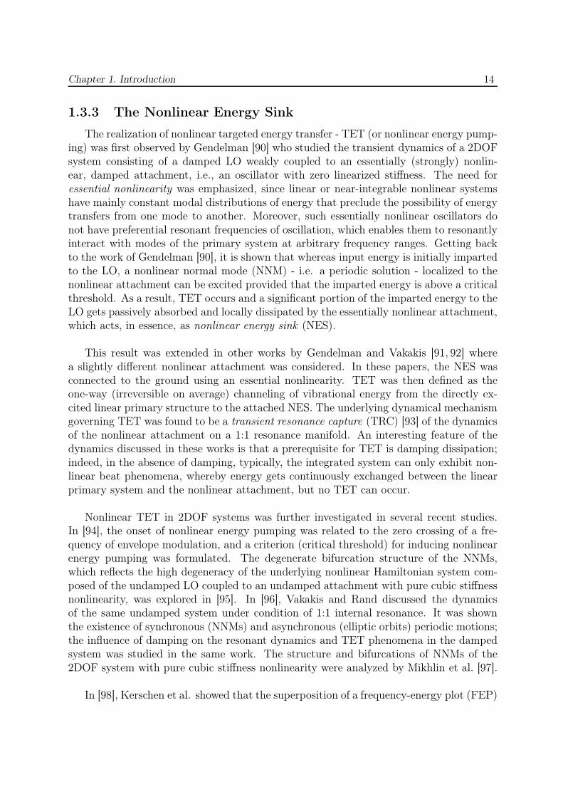
The realization of nonlinear targeted energy transfer - TET (or nonlinear energy pump-ing) was first observed by Gendelman [90] who studied the transient dynamics of a 2DOFsystem consisting of a damped LO weakly coupled to an essentially (strongly) nonlin-ear, damped attachment, i.e., an oscillator with zero linearized stiffness. The need foressential nonlinearity was emphasized, since linear or near-integrable nonlinear systemshave mainly constant modal distributions of energy that preclude the possibility of energytransfers from one mode to another. Moreover, such essentially nonlinear oscillators donot have preferential resonant frequencies of oscillation, which enables them to resonantlyinteract with modes of the primary system at arbitrary frequency ranges. Getting backto the work of Gendelman [90], it is shown that whereas input energy is initially impartedto the LO, a nonlinear normal mode (NNM) - i.e. a periodic solution - localized to thenonlinear attachment can be excited provided that the imparted energy is above a criticalthreshold. As a result, TET occurs and a significant portion of the imparted energy to theLO gets passively absorbed and locally dissipated by the essentially nonlinear attachment,which acts, in essence, as nonlinear energy sink (NES).
This result was extended in other works by Gendelman and Vakakis [91, 92] wherea slightly different nonlinear attachment was considered. In these papers, the NES wasconnected to the ground using an essential nonlinearity. TET was then defined as theone-way (irreversible on average) channeling of vibrational energy from the directly ex-cited linear primary structure to the attached NES. The underlying dynamical mechanismgoverning TET was found to be a transient resonance capture (TRC) [93] of the dynamicsof the nonlinear attachment on a 1:1 resonance manifold. An interesting feature of thedynamics discussed in these works is that a prerequisite for TET is damping dissipation;indeed, in the absence of damping, typically, the integrated system can only exhibit non-linear beat phenomena, whereby energy gets continuously exchanged between the linearprimary system and the nonlinear attachment, but no TET can occur.
Nonlinear TET in 2DOF systems was further investigated in several recent studies.In [94], the onset of nonlinear energy pumping was related to the zero crossing of a fre-quency of envelope modulation, and a criterion (critical threshold) for inducing nonlinearenergy pumping was formulated. The degenerate bifurcation structure of the NNMs,which reflects the high degeneracy of the underlying nonlinear Hamiltonian system com-posed of the undamped LO coupled to an undamped attachment with pure cubic stiffnessnonlinearity, was explored in [95]. In [96], Vakakis and Rand discussed the dynamicsof the same undamped system under condition of 1:1 internal resonance. It was shownthe existence of synchronous (NNMs) and asynchronous (elliptic orbits) periodic motions;the influence of damping on the resonant dynamics and TET phenomena in the dampedsystem was studied in the same work. The structure and bifurcations of NNMs of the2DOF system with pure cubic stiffness nonlinearity were analyzed by Mikhlin et al. [97].
In [98], Kerschen et al. showed that the superposition of a frequency-energy plot (FEP)
Chapter 1. Introduction 15
depicting the periodic orbits of the underlying Hamiltonian system to the wavelet trans-form (WT) spectra of the corresponding weakly damped responses represents a suitabletool for analyzing energy exchanges and transfers taking place in the damped system.A procedure for designing passive nonlinear energy pumping devices was developed byMusienko et al. [99] whereas the robustness of energy pumping in the presence of un-certain parameters was assessed by Gourdon and Lamarque [100]. In [101], Koz’min etal. performed studies on the optimal transfer of energy from a LO to a weakly coupledgrounded nonlinear attachment, using global optimization techniques. Additional the-oretical, numerical and experimental results on nonlinear TET were reported in recentworks from Gourdon et al. [102, 103].
The first experimental evidence of nonlinear energy pumping was provided by McFar-land et al. [104]. TRCs leading to TET were further analyzed experimentally by Kerschenet al. [105] whereas application of nonlinear energy pumping to problems in acoustics, wasdemonstrated experimentally by Cochelin et al. [106, 107].
In most of the aforementioned studies, grounded and relatively heavy nonlinear at-tachments (NESs) were considered, which clearly limits their applicability to practicalcases. Gendelman et al. [108] introduced a lightweight and ungrounded NES which ledto efficient nonlinear energy pumping from the LO to which it was attached. Althoughthere is no complete equivalence between the grounded and ungrounded NES, Kerschenet al. [98] showed that the governing equations (and dynamics) of these two NESs can berelated. In particular, an ungrounded NES with a small mass ratio ǫ and coupled throughessential nonlinearity to a LO is equivalent to a grounded NES with a large mass ratio(1+ǫ)/ǫ and stiff grounding nonlinearity.
The coming sections aim to present the essential characteristics related to the dynam-ics of an ungrounded NES coupled to linear SDOF, MDOF and nonlinear systems.
1.3.3.1 Linear Single-Degree-of-Freedom Primary Structure
The dynamics of a 2DOF system composed of a LO coupled to an ungrounded andlight-weight NES was analyzed in a series of recent papers [109–112]. The related resultsare of particular interest as the structural configuration can directly be compared to thatof a LO coupled to a TMD.
Energy Dissipation in the Damped System
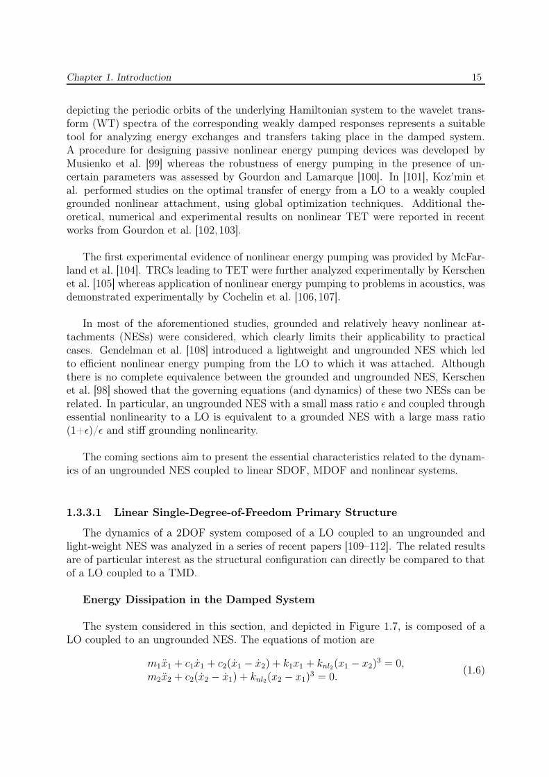
The system considered in this section, and depicted in Figure 1.7, is composed of aLO coupled to an ungrounded NES. The equations of motion are
m1x1 + c1x1 + c2(x1 − x2) + k1x1 + knl2(x1 − x2)3 = 0,
m2x2 + c2(x2 − x1) + knl2(x2 − x1)3 = 0.
(1.6)
Chapter 1. Introduction 16
k1
c1
knl2
c2
m1 m2
x1
x2
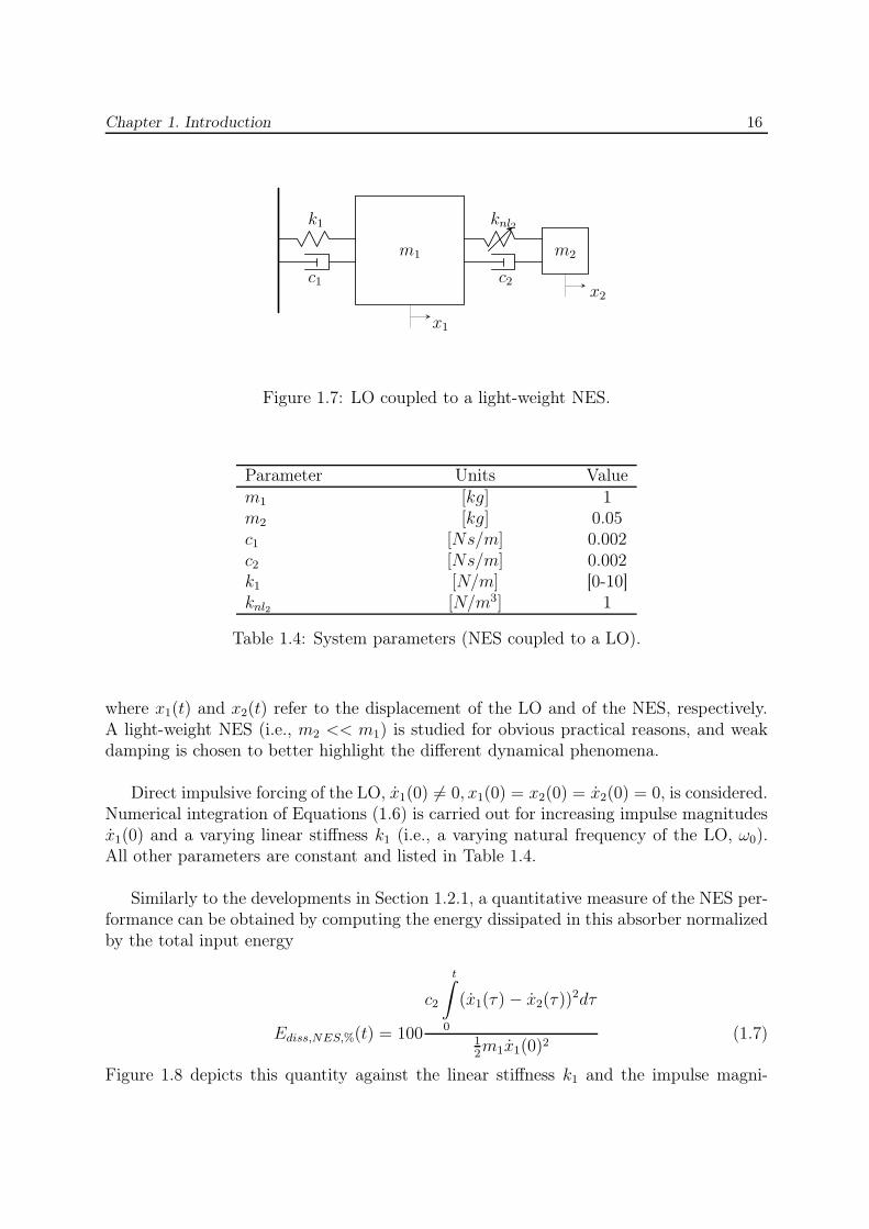
Figure 1.7: LO coupled to a light-weight NES.
Parameter Units Valuem1 [kg] 1m2 [kg] 0.05c1 [Ns/m] 0.002c2 [Ns/m] 0.002k1 [N/m] [0-10]knl2 [N/m3] 1
Table 1.4: System parameters (NES coupled to a LO).
where x1(t) and x2(t) refer to the displacement of the LO and of the NES, respectively.A light-weight NES (i.e., m2 << m1) is studied for obvious practical reasons, and weakdamping is chosen to better highlight the different dynamical phenomena.
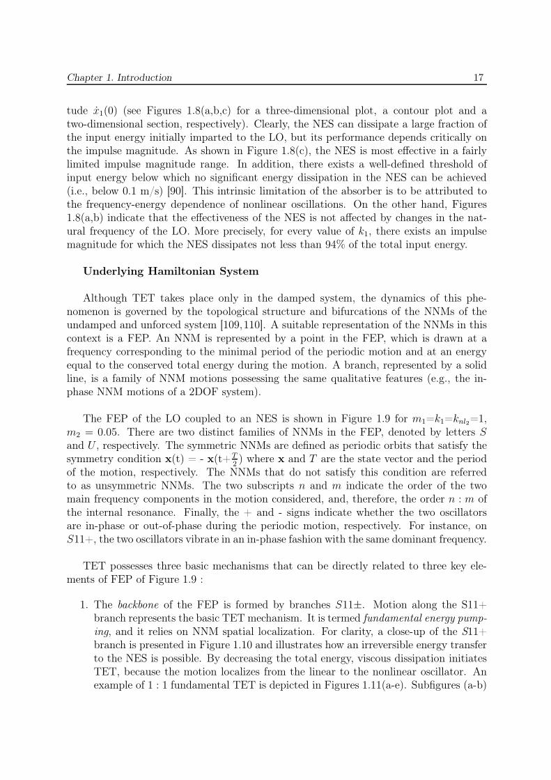
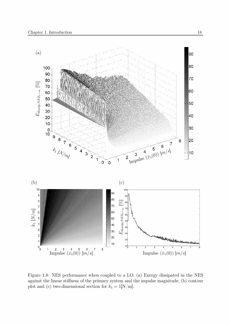
Direct impulsive forcing of the LO, x1(0) 6= 0, x1(0) = x2(0) = x2(0) = 0, is considered.Numerical integration of Equations (1.6) is carried out for increasing impulse magnitudesx1(0) and a varying linear stiffness k1 (i.e., a varying natural frequency of the LO, ω0).All other parameters are constant and listed in Table 1.4.
Similarly to the developments in Section 1.2.1, a quantitative measure of the NES per-formance can be obtained by computing the energy dissipated in this absorber normalizedby the total input energy
Ediss,NES,%(t) = 100
c2
t∫
0
(x1(τ) − x2(τ))2dτ
12m1x1(0)2
(1.7)
Figure 1.8 depicts this quantity against the linear stiffness k1 and the impulse magni-
Chapter 1. Introduction 17
tude x1(0) (see Figures 1.8(a,b,c) for a three-dimensional plot, a contour plot and atwo-dimensional section, respectively). Clearly, the NES can dissipate a large fraction ofthe input energy initially imparted to the LO, but its performance depends critically onthe impulse magnitude. As shown in Figure 1.8(c), the NES is most effective in a fairlylimited impulse magnitude range. In addition, there exists a well-defined threshold ofinput energy below which no significant energy dissipation in the NES can be achieved(i.e., below 0.1 m/s) [90]. This intrinsic limitation of the absorber is to be attributed tothe frequency-energy dependence of nonlinear oscillations. On the other hand, Figures1.8(a,b) indicate that the effectiveness of the NES is not affected by changes in the nat-ural frequency of the LO. More precisely, for every value of k1, there exists an impulsemagnitude for which the NES dissipates not less than 94% of the total input energy.
Underlying Hamiltonian System
Although TET takes place only in the damped system, the dynamics of this phe-nomenon is governed by the topological structure and bifurcations of the NNMs of theundamped and unforced system [109,110]. A suitable representation of the NNMs in thiscontext is a FEP. An NNM is represented by a point in the FEP, which is drawn at afrequency corresponding to the minimal period of the periodic motion and at an energyequal to the conserved total energy during the motion. A branch, represented by a solidline, is a family of NNM motions possessing the same qualitative features (e.g., the in-phase NNM motions of a 2DOF system).
The FEP of the LO coupled to an NES is shown in Figure 1.9 for m1=k1=knl2=1,m2 = 0.05. There are two distinct families of NNMs in the FEP, denoted by letters Sand U , respectively. The symmetric NNMs are defined as periodic orbits that satisfy thesymmetry condition x(t) = - x(t+T
2) where x and T are the state vector and the period
of the motion, respectively. The NNMs that do not satisfy this condition are referredto as unsymmetric NNMs. The two subscripts n and m indicate the order of the twomain frequency components in the motion considered, and, therefore, the order n : m ofthe internal resonance. Finally, the + and - signs indicate whether the two oscillatorsare in-phase or out-of-phase during the periodic motion, respectively. For instance, onS11+, the two oscillators vibrate in an in-phase fashion with the same dominant frequency.
TET possesses three basic mechanisms that can be directly related to three key ele-ments of FEP of Figure 1.9 :
1. The backbone of the FEP is formed by branches S11±. Motion along the S11+branch represents the basic TET mechanism. It is termed fundamental energy pump-ing, and it relies on NNM spatial localization. For clarity, a close-up of the S11+branch is presented in Figure 1.10 and illustrates how an irreversible energy transferto the NES is possible. By decreasing the total energy, viscous dissipation initiatesTET, because the motion localizes from the linear to the nonlinear oscillator. Anexample of 1 : 1 fundamental TET is depicted in Figures 1.11(a-e). Subfigures (a-b)
Chapter 1. Introduction 18
Impulse (x1(0)) [m/s]
k1 [N/m]
Edis
sip,N
ES
t→
∞[%
]
(a)
0 1 2 3 4 5 6 7 810
20
30
40
50
60
70
80
90
100
Impulse (x1(0)) [m/s]Impulse (x1(0)) [m/s]
k1
[N/m
]
(b)
Edis
sip,N
ES
t→
∞[%
]
(c)
Figure 1.8: NES performance when coupled to a LO. (a) Energy dissipated in the NESagainst the linear stiffness of the primary system and the impulse magnitude; (b) contourplot and (c) two-dimensional section for k1 = 1[N/m].
Chapter 1. Introduction 19
10-6 10-5 10-4 10-3 10-2 10-1 100 1010,0
0,5
1,0
1,5
2,0
2,5
3,0
S31
U21
S11−
U32
U12
S13U14
S15
S11+Puls
atio
n[r
ad/s
]
Energy [log]
Manifold ofImpulsive
orbits
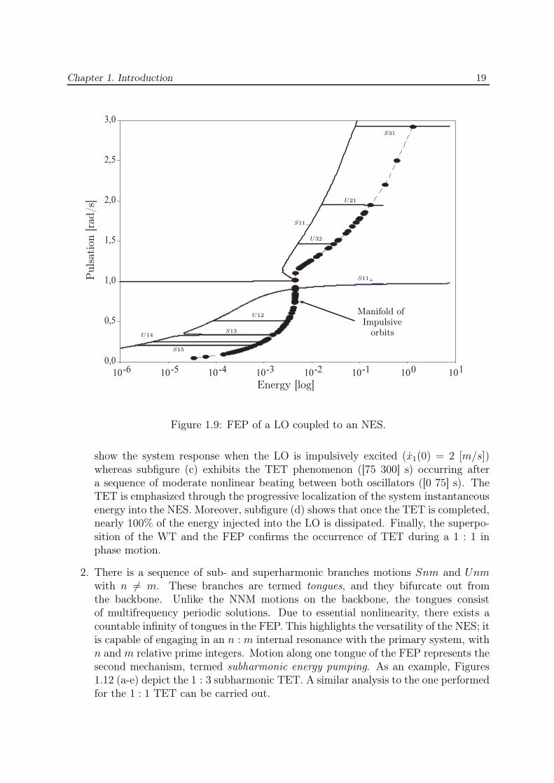
Figure 1.9: FEP of a LO coupled to an NES.
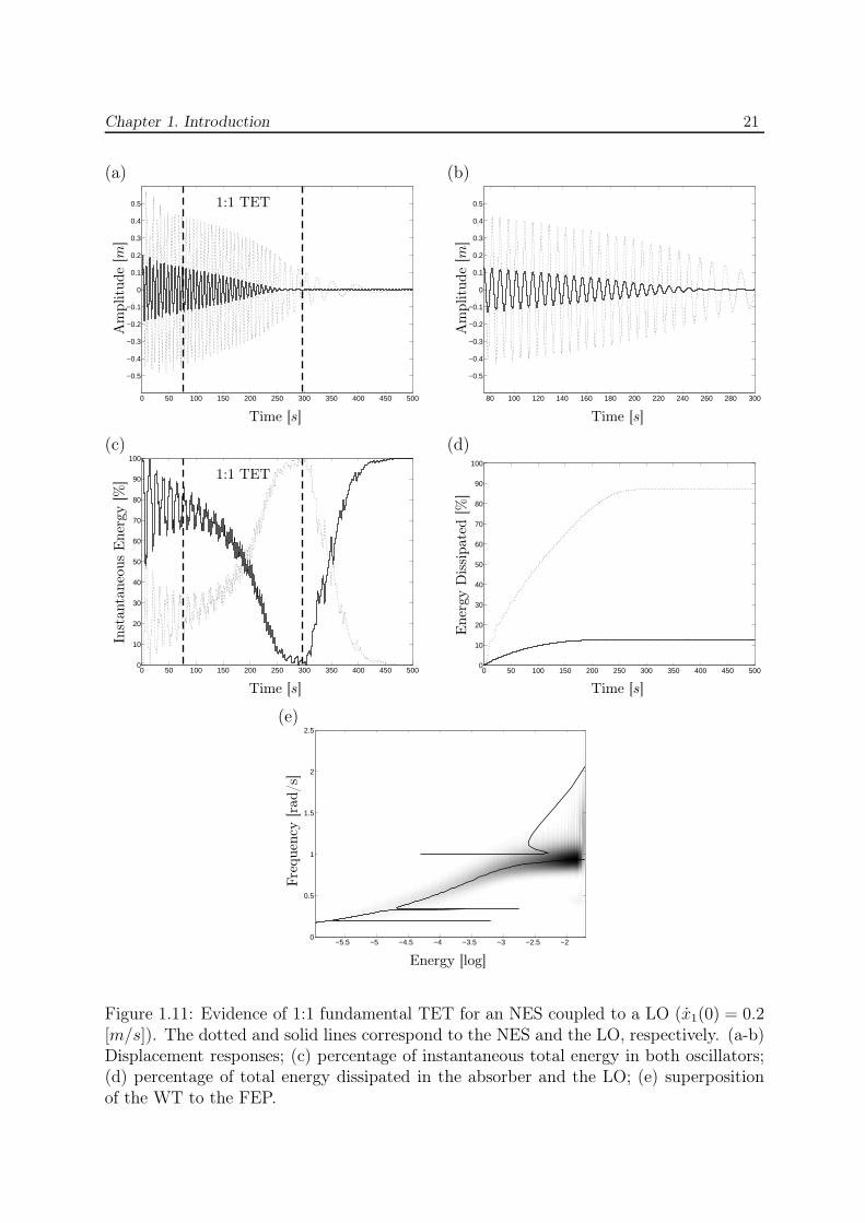
show the system response when the LO is impulsively excited (x1(0) = 2 [m/s])whereas subfigure (c) exhibits the TET phenomenon ([75 300] s) occurring aftera sequence of moderate nonlinear beating between both oscillators ([0 75] s). TheTET is emphasized through the progressive localization of the system instantaneousenergy into the NES. Moreover, subfigure (d) shows that once the TET is completed,nearly 100% of the energy injected into the LO is dissipated. Finally, the superpo-sition of the WT and the FEP confirms the occurrence of TET during a 1 : 1 inphase motion.
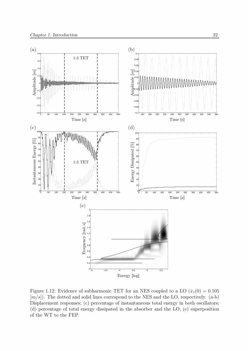
2. There is a sequence of sub- and superharmonic branches motions Snm and Unmwith n 6= m. These branches are termed tongues, and they bifurcate out fromthe backbone. Unlike the NNM motions on the backbone, the tongues consistof multifrequency periodic solutions. Due to essential nonlinearity, there exists acountable infinity of tongues in the FEP. This highlights the versatility of the NES; itis capable of engaging in an n : m internal resonance with the primary system, withn and m relative prime integers. Motion along one tongue of the FEP represents thesecond mechanism, termed subharmonic energy pumping. As an example, Figures1.12 (a-e) depict the 1 : 3 subharmonic TET. A similar analysis to the one performedfor the 1 : 1 TET can be carried out.
Chapter 1. Introduction 20
Fre
quen
cyIn
dex
[rad/s]
Total energy [log]
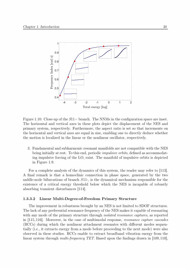
Figure 1.10: Close-up of the S11+ branch. The NNMs in the configuration space are inset.The horizontal and vertical axes in these plots depict the displacement of the NES andprimary system, respectively. Furthermore, the aspect ratio is set so that increments onthe horizontal and vertical axes are equal in size, enabling one to directly deduce whetherthe motion is localized in the linear or the nonlinear oscillator, respectively.
3. Fundamental and subharmonic resonant manifolds are not compatible with the NESbeing initially at rest. To this end, periodic impulsive orbits, defined as accommodat-ing impulsive forcing of the LO, exist. The manifold of impulsive orbits is depictedin Figure 1.9.
For a complete analysis of the dynamics of this system, the reader may refer to [113].A final remark is that a homoclinic connection in phase space, generated by the twosaddle-node bifurcations of branch S11-, is the dynamical mechanism responsible for theexistence of a critical energy threshold below which the NES is incapable of robustlyabsorbing transient disturbances [114].
1.3.3.2 Linear Multi-Degree-of-Freedom Primary Structure
The improvement in robustness brought by an NES is not limited to SDOF structures.The lack of any preferential resonance frequency of the NES makes it capable of resonatingwith any mode of the primary structure through isolated resonance captures, as reportedin [115, 116]. Moreover, in the case of multimodal response, resonance capture cascades(RCCs) during which the nonlinear attachment resonates with different modes sequen-tially (i.e., it extracts energy from a mode before proceeding to the next mode) were alsoobserved in these studies. RCCs enable to extract broadband vibration energy from thelinear system through multi-frequency TET. Based upon the findings drawn in [109,110],
Chapter 1. Introduction 21
0 50 100 150 200 250 300 350 400 450 500
−0.5
−0.4
−0.3
−0.2
−0.1
0
0.1
0.2
0.3
0.4
0.5
Time [s]
Am
plitu
de
[m]
(a)
80 100 120 140 160 180 200 220 240 260 280 300
−0.5
−0.4
−0.3
−0.2
−0.1
0
0.1
0.2
0.3
0.4
0.5
Time [s]
Am
plitu
de
[m]
(b)
0 50 100 150 200 250 300 350 400 450 5000
10
20
30
40
50
60
70
80
90
100
Time [s]
Inst
anta
neo
us
Ener
gy
[%]
(c)
0 50 100 150 200 250 300 350 400 450 5000
10
20
30
40
50
60
70
80
90
100
Time [s]
Ener
gy
Dis
sipate
d[%
](d)
−5.5 −5 −4.5 −4 −3.5 −3 −2.5 −20
0.5
1
1.5
2
2.5
Energy [log]
Fre
quen
cy[r
ad/s]
(e)
1:1 TET
1:1 TET
Figure 1.11: Evidence of 1:1 fundamental TET for an NES coupled to a LO (x1(0) = 0.2[m/s]). The dotted and solid lines correspond to the NES and the LO, respectively. (a-b)Displacement responses; (c) percentage of instantaneous total energy in both oscillators;(d) percentage of total energy dissipated in the absorber and the LO; (e) superpositionof the WT to the FEP.
Chapter 1. Introduction 22
0 50 100 150 200 250 300 350 400 450 500−0.4
−0.3
−0.2
−0.1
0
0.1
0.2
0.3
0.4
Time [s]
Am
plitu
de
[m]
(a)
160 180 200 220 240 260 280 300 320 340 360−0.1
−0.08
−0.06
−0.04
−0.02
0
0.02
0.04
0.06
0.08
0.1
Time [s]
Am
plitu
de
[m]
(b)
0 50 100 150 200 250 300 350 400 450 5000
10
20
30
40
50
60
70
80
90
100
Time [s]
Inst
anta
neo
us
Ener
gy
[%]
(c)
0 50 100 150 200 250 300 350 400 450 5000
10
20
30
40
50
60
70
80
90
100
Time [s]
Ener
gy
Dis
sipate
d[%
](d)
−5 −4.5 −4 −3.5 −3 −2.50
0.2
0.4
0.6
0.8
1
1.2
1.4
1.6
1.8
2
Energy [log]
Fre
quen
cy[r
ad/s]
(e)
1:3 TET
1:3 TET
Figure 1.12: Evidence of subharmonic TET for an NES coupled to a LO (x1(0) = 0.105[m/s]). The dotted and solid lines correspond to the NES and the LO, respectively. (a-b)Displacement responses; (c) percentage of instantaneous total energy in both oscillators;(d) percentage of total energy dissipated in the absorber and the LO; (e) superpositionof the WT to the FEP.
Chapter 1. Introduction 23
TET occurring between a 2DOF structure and an NES were described in [117].
As an example, let us consider the 6DOF system composed of a 5DOF linear primarystructure coupled to a SDOF NES. The related equations of motion are given by :
x1 + 0.014x1 + 2x1 − x2 = 0x2 + 0.014x2 + 2x2 − x1 − x3 = 0x3 + 0.014x3 + 2x3 − x2 − x4 = 0x4 + 0.014x4 + 2x4 − x3 − x5 = 0x5 + 0.014x5 − 0.0001ν + 2x5 − x4 + (x5 − ν)3 = 00.05ν + 0.0001(ν − x5) + (ν − x5)
3 = 0
(1.8)
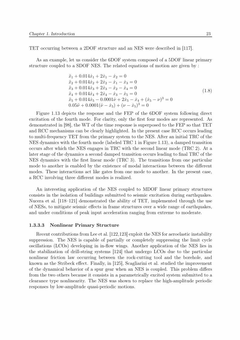
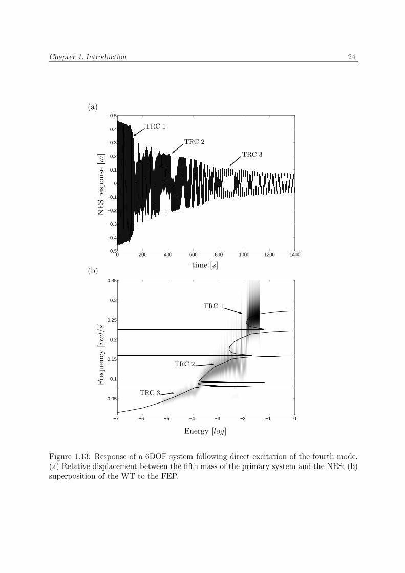
Figure 1.13 depicts the response and the FEP of the 6DOF system following directexcitation of the fourth mode. For clarity, only the first four modes are represented. Asdemonstrated in [98], the WT of the time response is superposed to the FEP so that TETand RCC mechanisms can be clearly highlighted. In the present case RCC occurs leadingto multi-frequency TET from the primary system to the NES. After an initial TRC of theNES dynamics with the fourth mode (labeled TRC 1 in Figure 1.13), a damped transitionoccurs after which the NES engages in TRC with the second linear mode (TRC 2). At alater stage of the dynamics a second damped transition occurs leading to final TRC of theNES dynamics with the first linear mode (TRC 3). The transitions from one particularmode to another is enabled by the existence of modal interactions between the differentmodes. These interactions act like gates from one mode to another. In the present case,a RCC involving three different modes is realized.
An interesting application of the NES coupled to MDOF linear primary structuresconsists in the isolation of buildings submitted to seismic excitation during earthquakes.Nucera et al. [118–121] demonstrated the ability of TET, implemented through the useof NESs, to mitigate seismic effects in frame structures over a wide range of earthquakes,and under conditions of peak input acceleration ranging from extreme to moderate.
1.3.3.3 Nonlinear Primary Structure
Recent contributions from Lee et al. [122,123] exploit the NES for aeroelastic instabilitysuppression. The NES is capable of partially or completely suppressing the limit cycleoscillations (LCOs) developing in in-flow wings. Another application of the NES lies inthe stabilization of drill-string systems [124] that undergo LCOs due to the particularnonlinear friction law occurring between the rock-cutting tool and the borehole, andknown as the Stribeck effect. Finally, in [125], Scagliarini et al. studied the improvementof the dynamical behavior of a spur gear when an NES is coupled. This problem differsfrom the two others because it consists in a parametrically excited system submitted to aclearance type nonlinearity. The NES was shown to replace the high-amplitude periodicresponses by low-amplitude quasi-periodic motions.
Chapter 1. Introduction 24
0 200 400 600 800 1000 1200 1400−0.5
−0.4
−0.3
−0.2
−0.1
0
0.1
0.2
0.3
0.4
0.5
−7 −6 −5 −4 −3 −2 −1 0
0.05
0.1
0.15
0.2
0.25
0.3
0.35
time [s]
NE
Sre
spon
se[m
](a)
Energy [log]
Fre
quen
cy[r
ad/s
]
(b)
TRC 1
TRC 2
TRC 3
TRC 1
TRC 2
TRC 3
Figure 1.13: Response of a 6DOF system following direct excitation of the fourth mode.(a) Relative displacement between the fifth mass of the primary system and the NES; (b)superposition of the WT to the FEP.
Chapter 1. Introduction 25
1.4 Motivation of this Doctoral Dissertation
As discussed in Sections 1.2 and 1.3, a large body of literature exists regarding linearand nonlinear dynamic absorbers, but the vast majority of it deals with linear primarystructures. However, nonlinearity is a frequency occurrence in engineering applications.For instance, in an aircraft, besides nonlinear fluid-structure interaction, typical non-linearities include backlash and friction in control surfaces, hardening nonlinearities inengine-to-pylon connections, saturation effects in hydraulic actuators, plus any underly-ing distributed nonlinearity in the structure.
The present thesis focuses on the mitigation of vibrations of nonlinear primary systemsusing nonlinear dynamic absorbers. One potential limitation of these absorbers is thattheir performance depends critically on the total energy present in the system or, equiv-alently, on the amplitude of the external forcing. This stems from the frequency-energydependence of nonlinear oscillations, which is one typical feature of nonlinear dynamicalsystems. For instance, the NES is effective in a fairly limited range of impulse magni-tudes, as shown in Figure 1.8(c). A first objective of this thesis is therefore to developa nonlinear dynamic absorber that can mitigate the vibrations of a specific mode of anonlinear primary structure in a wide range of input energies.
In this context, it is interesting to note that the determination of an optimal functionalform for the absorber nonlinearity is rarely addressed in the literature. For instance, acubic stiffness is often selected, because its practical realization is fairly simple. A secondobjective of the thesis is to propose a tuning procedure, which determines the absorberparameters (i.e., mass, damping and stiffness) together with an appropriate functionalform for the absorber nonlinearity. Because most existing contributions about the designof NLVAs rely on optimization and sensitivity analysis procedures (e.g., [20, 126–128]),which are computationally demanding, or on analytic methods, which may be limited tosmall-amplitude motions, a particular attention will be paid so that the tuning procedurecan be computationally tractable and treat strongly nonlinear regimes of motion.
1.5 Outline of the Thesis
The first part of the thesis (Chapters 2 to 5) is devoted to the development of a tuningmethodology of NLVAs coupled to nonlinear mechanical structures.
Chapter 2 characterizes the dynamics created by the coupling of a grounded Duffingoscillator and an NES. The underlying Hamiltonian system is first considered and thefundamental dynamics of the strongly nonlinear 2DOF is analyzed. The damped systemis then investigated and the basic mechanisms for energy transfer and dissipation areanalyzed. This study aims to highlight essential properties that will be exploited for thetuning of an amplitude-robust NLVA.
Chapter 1. Introduction 26
Chapter 3 addresses the development of a qualitative tuning procedure to enlarge therange of input energies for which a NLVA is effective. In particular, an optimal functionalform for the NLVA is sought. The proposed methodology arises from an analogy with thetuning of a TMD coupled with a LO, and is based on the frequency-energy dependence ofboth nonlinear oscillators. The findings are then validated using a quantitative approachin which a nonlinear oscillator is coupled to different DVAs possessing various functionalforms.
The dynamics of an essentially nonlinear 2DOF homogeneous system is investigatedin Chapter 4. In particular, the emphasis is set upon the analysis of a linear-like behavioras well as energy-invariant NNMs taking place in these systems. They appear to play animportant role in the amplitude-robustness property of the developed NLVA.
Finally, Chapter 5 extends the frequency-energy-based tuning methodology to the caseof forced oscillations using bifurcation analysis. In particular, the tracking of bifurcationsis achieved in the parameter space so that accurate values of the NLVA stiffness anddamping coefficients are determined.
The second part of the thesis (Chapters 6 and 7) discusses the challenges that are stillto be addressed and highlights future research directions.
Chapter 6 focuses on the tuning of a NLVA to suppress self-sustained vibrations, alsocalled limit cycle oscillations (LCOs), arising in systems presenting nonlinear damping. Inparticular, the case of torsional vibrations occurring in drill-string systems is investigatedin detail.
Chapter 7 addresses the practical realization of a NLVA. The tuning procedure devel-oped in the first part of the thesis may lead to NLVAs possessing complicated nonlinearfunctional forms which may be difficult to realize mechanically. In this context, the devel-opment of nonlinear piezoelectric shunting strategies is relevant, because electrical circuitsmay enable the realization of nearly any nonlinear functional forms. A preliminary anal-ysis is performed using a beam coupled to an electrical NLVA.
Finally, conclusions regarding the completed research and the associated contributionsto the field are drawn. A discussion of the ways in which this research may be extendedis also given.
Chapter 2
Energy Transfer and Dissipation in a
Duffing Oscillator Coupled to a
Nonlinear Attachment
Abstract
The dynamics of a two-degree-of-freedom nonlinear system consisting of agrounded Duffing oscillator coupled to an ungrounded essentially nonlinearattachment is examined in the present chapter. The underlying Hamiltoniansystem is first considered, and its nonlinear normal modes are computed us-ing numerical continuation and gathered in a frequency-energy plot. Basedon these results, the damped system is considered, and the basic mechanismsfor energy transfer and dissipation are analyzed. Throughout this chapter theemphasis is set upon the comparison with the dynamics of a linear oscillatorcoupled to an essentially nonlinear attachment reviewed in Section 1.3.3.
27
Chapter 2. Duffing Oscillator coupled to a Nonlinear Attachment 28
2.1 Introduction
As reported in Section 1.3.3.1, even dynamical systems of simple configuration (suchas a linear oscillator (LO)) possess very rich and complicated dynamics when an essen-tially nonlinear oscillator (NES) is attached to them (see, e.g., [109]). An appropriatetheoretical framework, including analytic developments [91, 92], nonlinear normal mode(NNM) computation [109], and time-frequency analysis [110], was necessary to get a pro-found understanding of these complex phenomena.
As mentioned in Section 1.3.3, the vast majority of existing studies about the NESexamined its dynamics when coupled to linear primary structures. Moreover, because ofthe frequency-energy dependence of their oscillations, the use of a nonlinear absorber tomitigate the vibrations of nonlinear primary systems seems to be particularly relevant.This is why the present chapter builds upon the existing theoretical framework to carefullyanalyze the dynamics of a Duffing oscillator attached to an NES, and highlight fundamen-tal properties. Among the other contributions of this study, we note that a more robustalgorithm for the NNM computation is utilized. This algorithm was first proposed in [129]and relies on the combination of a shooting algorithm with pseudo-arclength continuation,as detailed in Appendix B.
2.2 Dynamics of a Duffing Oscillator Coupled to a Non-
linear Energy Sink
2.2.1 Nonlinear Energy Sink Performance
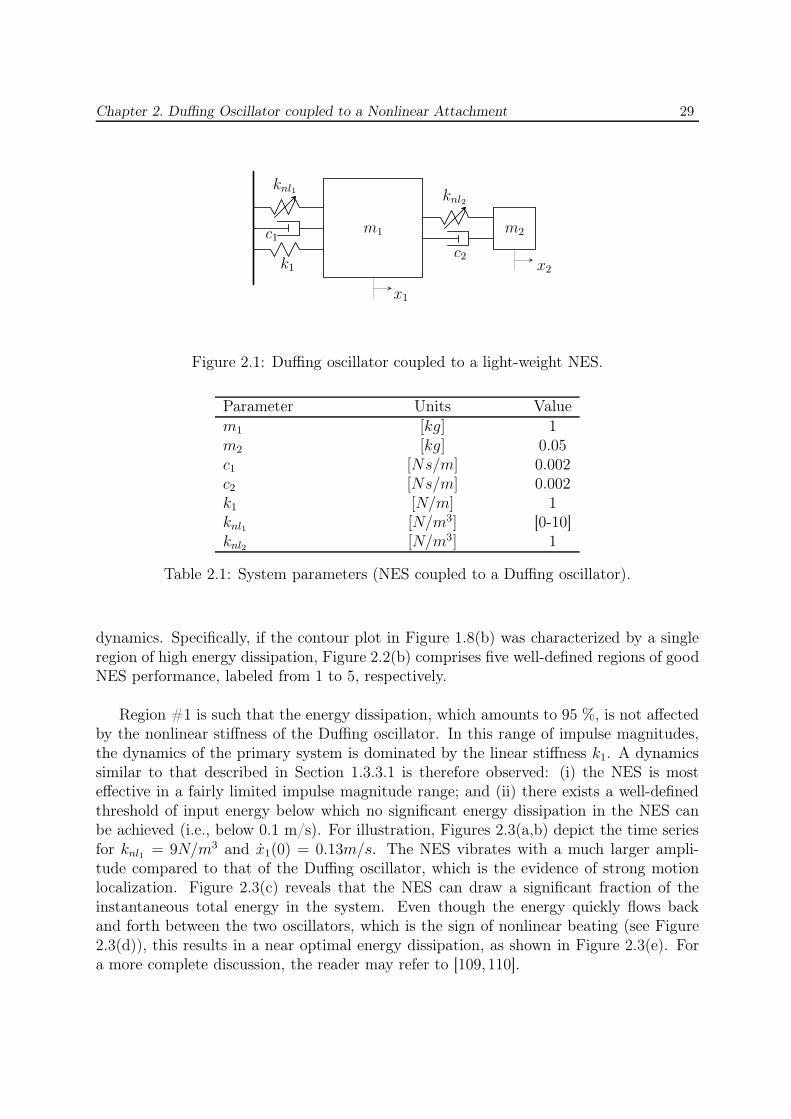
The performance of a nonlinear energy sink (NES) coupled to a nonlinear primarysystem is investigated. The system is depicted in Figure 2.1 and its equations of motionare given by :
m1x1 + c1x1 + c2(x1 − x2) + k1x1 + knl1x31 + knl2(x1 − x2)
3 = 0,m2x2 + c2(x2 − x1) + knl2(x2 − x1)
3 = 0.(2.1)
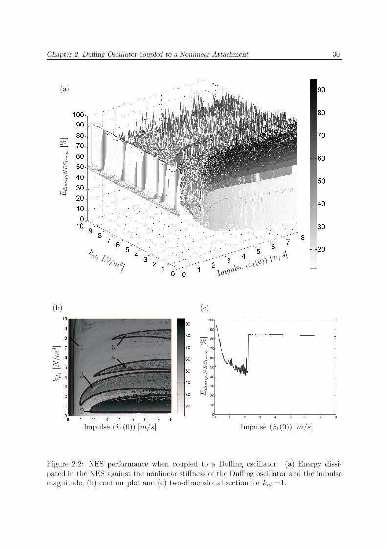
Direct impulsive forcing of the Duffing oscillator is considered by imposing a non-zero ini-tial velocity of the primary structure : x1(0) 6= 0, x1(0) = x2(0) = x2(0) = 0. The systemparameters are given in Table 2.1 and, based upon the formula established in Equation(1.7), the amount of energy initially imparted to the Duffing oscillator and dissipated inthe absorber can be determined.
Figure 2.2 depicts the energy dissipated in the NES against the impulse magnitudex1(0) and the nonlinear stiffness knl1 of the primary system (see Figures 2.2(a,b,c) for athree-dimensional plot, a contour plot and a two-dimensional section, respectively). Itappears that the NES can dissipate a large fraction of the input energy initially impartedto the Duffing oscillator. The comparison of Figures 1.8 and 2.2 reveals that the intro-duction of a nonlinear stiffness in the primary system gives rise to fundamentally different
Chapter 2. Duffing Oscillator coupled to a Nonlinear Attachment 29
knl1
c1
k1
knl2
c2
m1 m2
x1
x2
Figure 2.1: Duffing oscillator coupled to a light-weight NES.
Parameter Units Valuem1 [kg] 1m2 [kg] 0.05c1 [Ns/m] 0.002c2 [Ns/m] 0.002k1 [N/m] 1knl1 [N/m3] [0-10]knl2 [N/m3] 1
Table 2.1: System parameters (NES coupled to a Duffing oscillator).
dynamics. Specifically, if the contour plot in Figure 1.8(b) was characterized by a singleregion of high energy dissipation, Figure 2.2(b) comprises five well-defined regions of goodNES performance, labeled from 1 to 5, respectively.
Region #1 is such that the energy dissipation, which amounts to 95 %, is not affectedby the nonlinear stiffness of the Duffing oscillator. In this range of impulse magnitudes,the dynamics of the primary system is dominated by the linear stiffness k1. A dynamicssimilar to that described in Section 1.3.3.1 is therefore observed: (i) the NES is mosteffective in a fairly limited impulse magnitude range; and (ii) there exists a well-definedthreshold of input energy below which no significant energy dissipation in the NES canbe achieved (i.e., below 0.1 m/s). For illustration, Figures 2.3(a,b) depict the time seriesfor knl1 = 9N/m3 and x1(0) = 0.13m/s. The NES vibrates with a much larger ampli-tude compared to that of the Duffing oscillator, which is the evidence of strong motionlocalization. Figure 2.3(c) reveals that the NES can draw a significant fraction of theinstantaneous total energy in the system. Even though the energy quickly flows backand forth between the two oscillators, which is the sign of nonlinear beating (see Figure2.3(d)), this results in a near optimal energy dissipation, as shown in Figure 2.3(e). Fora more complete discussion, the reader may refer to [109, 110].
Chapter 2. Duffing Oscillator coupled to a Nonlinear Attachment 30
Impulse (x1(0)) [m/s]
knl1 [N/m 3]
Edis
sip,N
ES
t→
∞[%
]
(a)
0 1 2 3 4 5 6 7 80
10
20
30
40
50
60
70
80
90
100
Impulse (x1(0)) [m/s]Impulse (x1(0)) [m/s]
k,l1
[N/m
3]
(b)
Edis
sip,N
ES
t→
∞[%
]
(c)
2
3
54
1
Figure 2.2: NES performance when coupled to a Duffing oscillator. (a) Energy dissi-pated in the NES against the nonlinear stiffness of the Duffing oscillator and the impulsemagnitude; (b) contour plot and (c) two-dimensional section for knl1=1.
Chapter 2. Duffing Oscillator coupled to a Nonlinear Attachment 31
0 50 100 150 200 250 300 350 400 450 500
−0.1
−0.05
0
0.05
0.1
0.15
Time [s]
Am
plitu
de
[m]
(a)
0 50 100 150 200 250 300 350 400 450 500−0.5
−0.4
−0.3
−0.2
−0.1
0
0.1
0.2
0.3
0.4
0.5
Time [s]
Am
plitu
de
[m]
(b)
0 50 100 150 200 250 300 350 400 450 5000
10
20
30
40
50
60
70
80
90
100
Time [s]
Ein
stant,
NE
S[%
]
(c)
0 5 10 15 20 25 30 35 40 45 50−0.4
−0.3
−0.2
−0.1
0
0.1
0.2
0.3
0.4
0.5
Duffing OscillatorNES
Time [s]
Am
plitu
de
[m]
(d)
0 50 100 150 200 250 300 350 400 450 5000
10
20
30
40
50
60
70
80
90
100
Time [s]
Edis
sip,N
ES
[%]
(e)
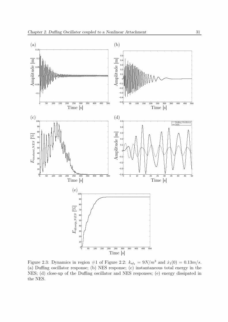
Figure 2.3: Dynamics in region #1 of Figure 2.2: knl1 = 9N/m3 and x1(0) = 0.13m/s.(a) Duffing oscillator response; (b) NES response; (c) instantaneous total energy in theNES; (d) close-up of the Duffing oscillator and NES responses; (e) energy dissipated inthe NES.
Chapter 2. Duffing Oscillator coupled to a Nonlinear Attachment 32
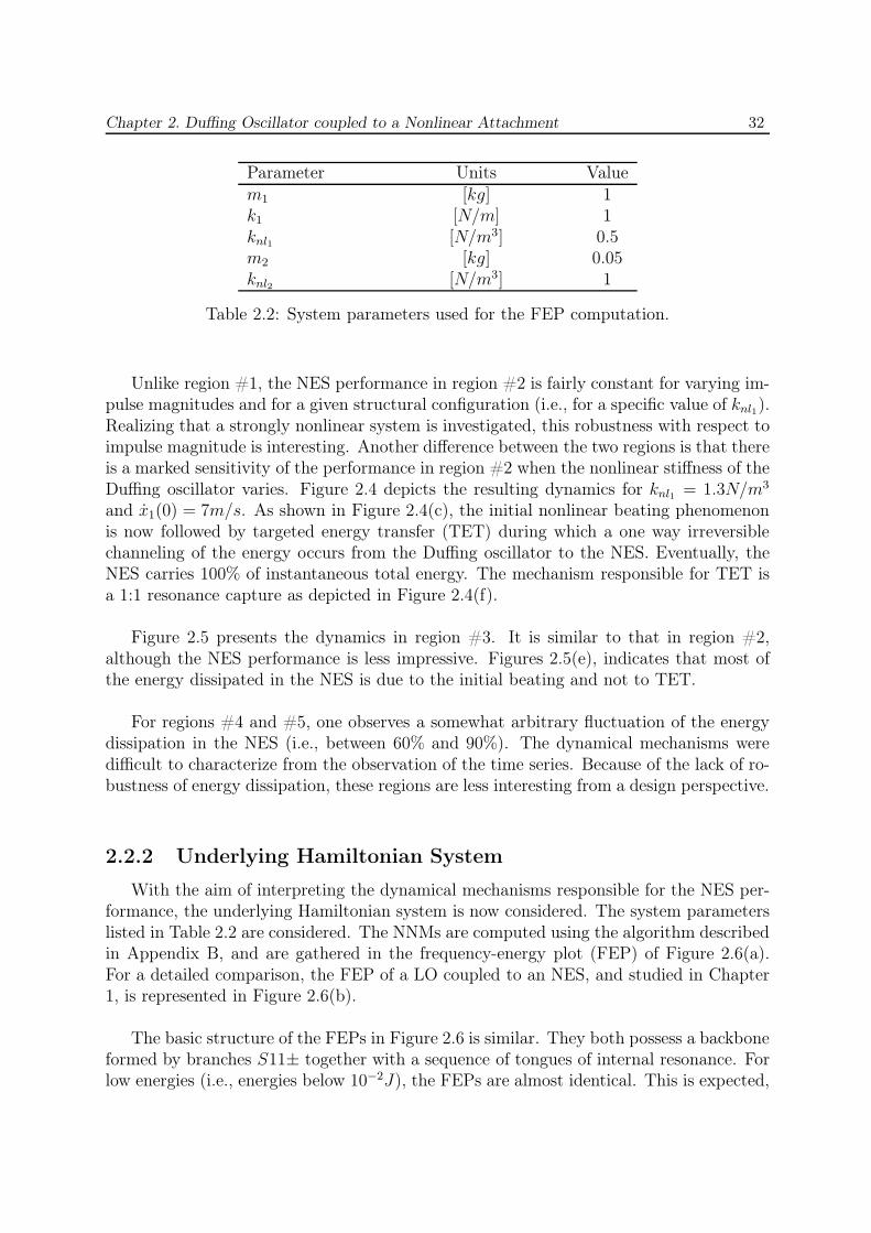
Parameter Units Valuem1 [kg] 1k1 [N/m] 1knl1 [N/m3] 0.5m2 [kg] 0.05knl2 [N/m3] 1
Table 2.2: System parameters used for the FEP computation.
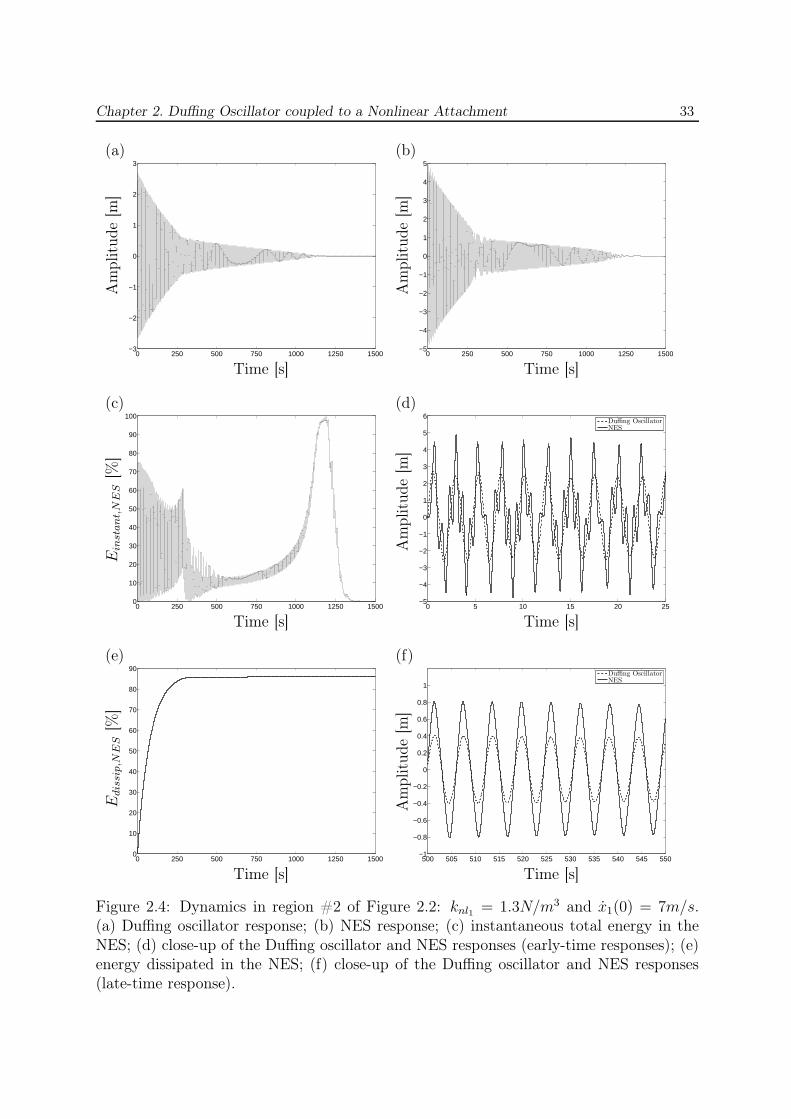
Unlike region #1, the NES performance in region #2 is fairly constant for varying im-pulse magnitudes and for a given structural configuration (i.e., for a specific value of knl1).Realizing that a strongly nonlinear system is investigated, this robustness with respect toimpulse magnitude is interesting. Another difference between the two regions is that thereis a marked sensitivity of the performance in region #2 when the nonlinear stiffness of theDuffing oscillator varies. Figure 2.4 depicts the resulting dynamics for knl1 = 1.3N/m3
and x1(0) = 7m/s. As shown in Figure 2.4(c), the initial nonlinear beating phenomenonis now followed by targeted energy transfer (TET) during which a one way irreversiblechanneling of the energy occurs from the Duffing oscillator to the NES. Eventually, theNES carries 100% of instantaneous total energy. The mechanism responsible for TET isa 1:1 resonance capture as depicted in Figure 2.4(f).
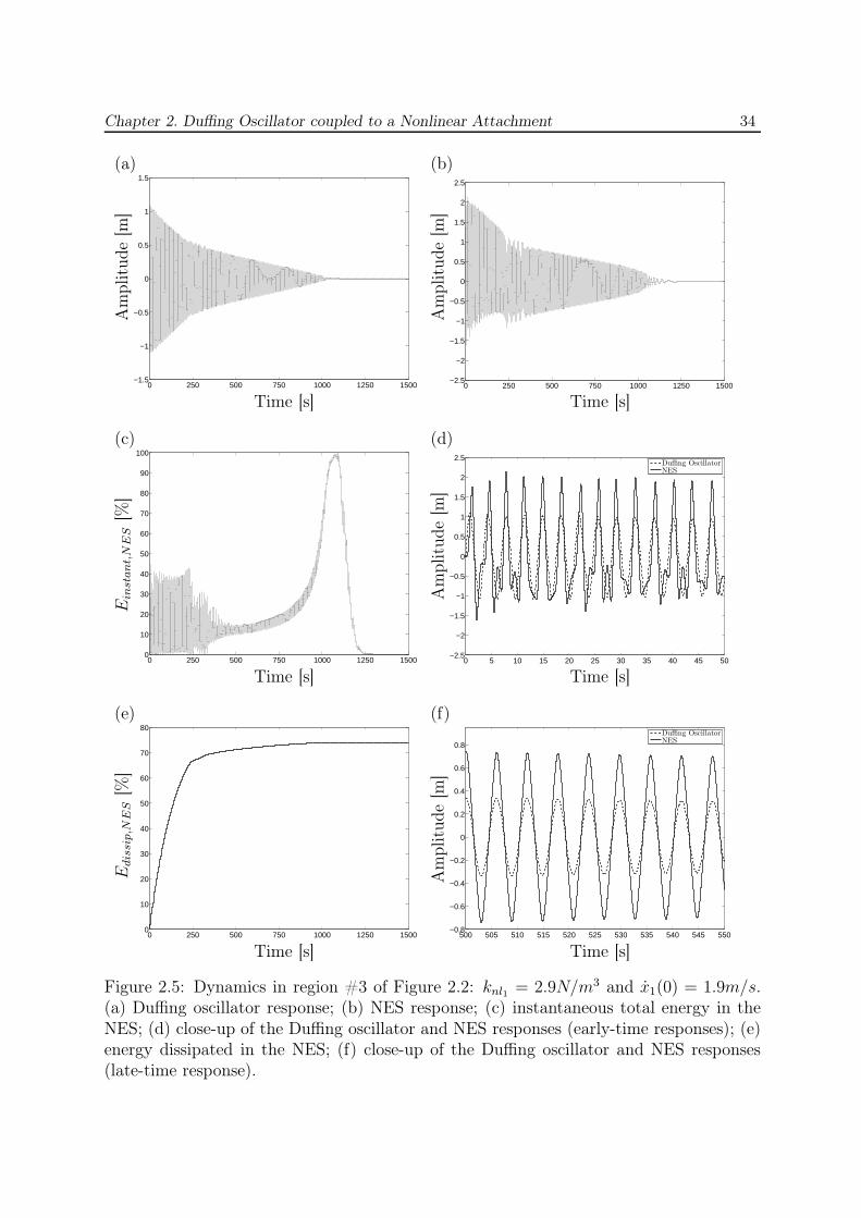
Figure 2.5 presents the dynamics in region #3. It is similar to that in region #2,although the NES performance is less impressive. Figures 2.5(e), indicates that most ofthe energy dissipated in the NES is due to the initial beating and not to TET.
For regions #4 and #5, one observes a somewhat arbitrary fluctuation of the energydissipation in the NES (i.e., between 60% and 90%). The dynamical mechanisms weredifficult to characterize from the observation of the time series. Because of the lack of ro-bustness of energy dissipation, these regions are less interesting from a design perspective.
2.2.2 Underlying Hamiltonian System
With the aim of interpreting the dynamical mechanisms responsible for the NES per-formance, the underlying Hamiltonian system is now considered. The system parameterslisted in Table 2.2 are considered. The NNMs are computed using the algorithm describedin Appendix B, and are gathered in the frequency-energy plot (FEP) of Figure 2.6(a).For a detailed comparison, the FEP of a LO coupled to an NES, and studied in Chapter1, is represented in Figure 2.6(b).
The basic structure of the FEPs in Figure 2.6 is similar. They both possess a backboneformed by branches S11± together with a sequence of tongues of internal resonance. Forlow energies (i.e., energies below 10−2J), the FEPs are almost identical. This is expected,
Chapter 2. Duffing Oscillator coupled to a Nonlinear Attachment 33
0 250 500 750 1000 1250 1500−3
−2
−1
0
1
2
3
Time [s]
Am
plitu
de
[m]
(a)
0 250 500 750 1000 1250 1500−5
−4
−3
−2
−1
0
1
2
3
4
5
Time [s]
Am
plitu
de
[m]
(b)
0 250 500 750 1000 1250 15000
10
20
30
40
50
60
70
80
90
100
Time [s]
Ein
stant,
NE
S[%
]
(c)
0 5 10 15 20 25−5
−4
−3
−2
−1
0
1
2
3
4
5
6
Duffing OscillatorNES
Time [s]
Am
plitu
de
[m]
(d)
0 250 500 750 1000 1250 15000
10
20
30
40
50
60
70
80
90
Time [s]
Edis
sip,N
ES
[%]
(e)
500 505 510 515 520 525 530 535 540 545 550−1
−0.8
−0.6
−0.4
−0.2
0
0.2
0.4
0.6
0.8
1
Duffing OscillatorNES
Time [s]
Am
plitu
de
[m]
(f)
Figure 2.4: Dynamics in region #2 of Figure 2.2: knl1 = 1.3N/m3 and x1(0) = 7m/s.(a) Duffing oscillator response; (b) NES response; (c) instantaneous total energy in theNES; (d) close-up of the Duffing oscillator and NES responses (early-time responses); (e)energy dissipated in the NES; (f) close-up of the Duffing oscillator and NES responses(late-time response).
Chapter 2. Duffing Oscillator coupled to a Nonlinear Attachment 34
0 250 500 750 1000 1250 1500−1.5
−1
−0.5
0
0.5
1
1.5
Time [s]
Am
plitu
de
[m]
(a)
0 250 500 750 1000 1250 1500−2.5
−2
−1.5
−1
−0.5
0
0.5
1
1.5
2
2.5
Time [s]
Am
plitu
de
[m]
(b)
0 250 500 750 1000 1250 15000
10
20
30
40
50
60
70
80
90
100
Time [s]
Ein
stant,
NE
S[%
]
(c)
0 5 10 15 20 25 30 35 40 45 50−2.5
−2
−1.5
−1
−0.5
0
0.5
1
1.5
2
2.5
Duffing OscillatorNES
Time [s]
Am
plitu
de
[m]
(d)
0 250 500 750 1000 1250 15000
10
20
30
40
50
60
70
80
Time [s]
Edis
sip,N
ES
[%]
(e)
500 505 510 515 520 525 530 535 540 545 550−0.8
−0.6
−0.4
−0.2
0
0.2
0.4
0.6
0.8
Duffing OscillatorNES
Time [s]
Am
plitu
de
[m]
(f)
Figure 2.5: Dynamics in region #3 of Figure 2.2: knl1 = 2.9N/m3 and x1(0) = 1.9m/s.(a) Duffing oscillator response; (b) NES response; (c) instantaneous total energy in theNES; (d) close-up of the Duffing oscillator and NES responses (early-time responses); (e)energy dissipated in the NES; (f) close-up of the Duffing oscillator and NES responses(late-time response).
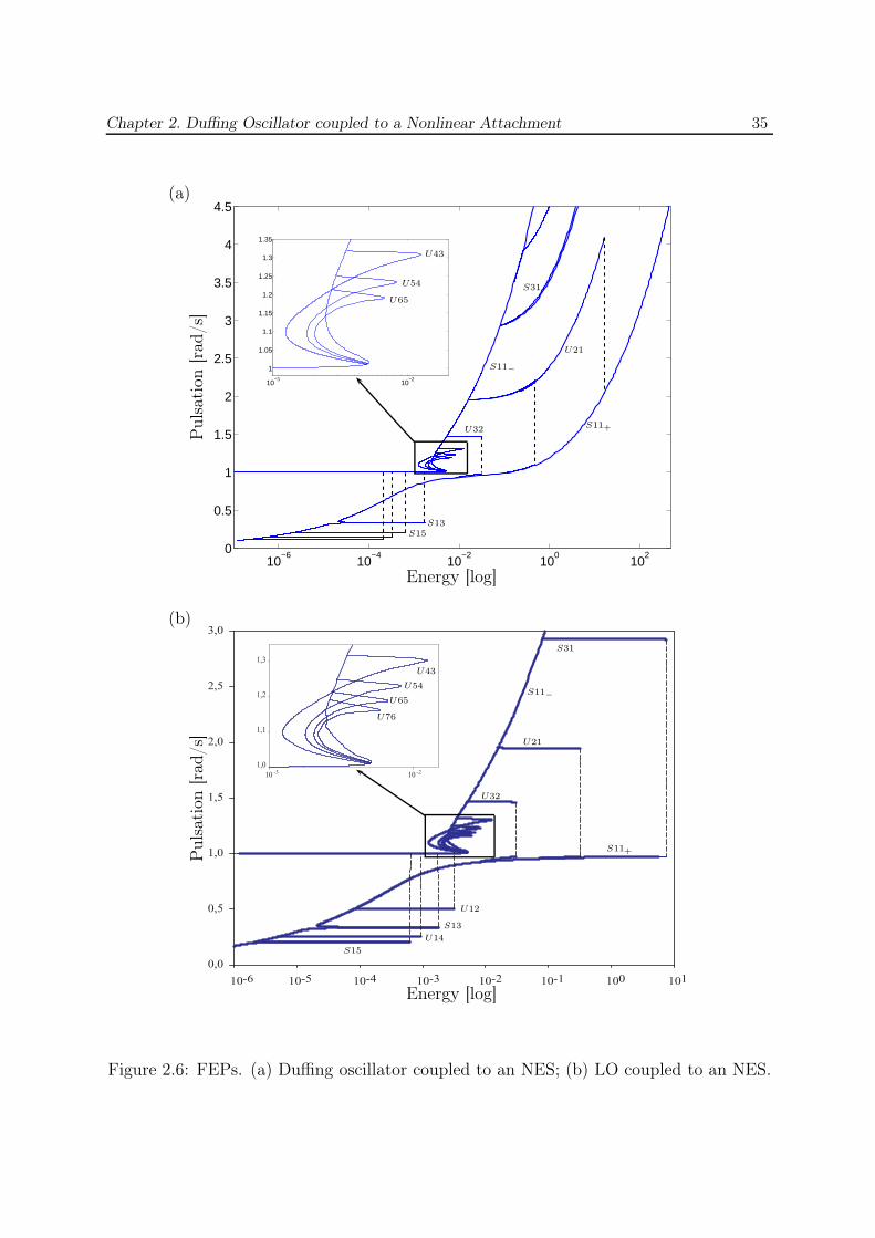
Chapter 2. Duffing Oscillator coupled to a Nonlinear Attachment 35
10-6
0,0
0,5
1,0
1,5
2,0
2,5
3,0
10-3
1,3
10-5 10-4 10-3 10-2 10-1 100 101
1,2
1,1
1,0
10-2
(b)
S31
U21
S11−
U32
U43
U54
U65
U76
U12
S13
U14
S15
S11+Puls
atio
n[r
ad/s
]
Energy [log]
10−6
10−4
10−2
100
1020
0.5
1
1.5
2
2.5
3
3.5
4
4.5
10−3
10−2
1
1.05
1.1
1.15
1.2
1.25
1.3
1.35
(a)
S31
U21
S11−
U32
U43
U54
U65
S13S15
S11+
Puls
atio
n[r
ad/s
]
Energy [log]
Figure 2.6: FEPs. (a) Duffing oscillator coupled to an NES; (b) LO coupled to an NES.
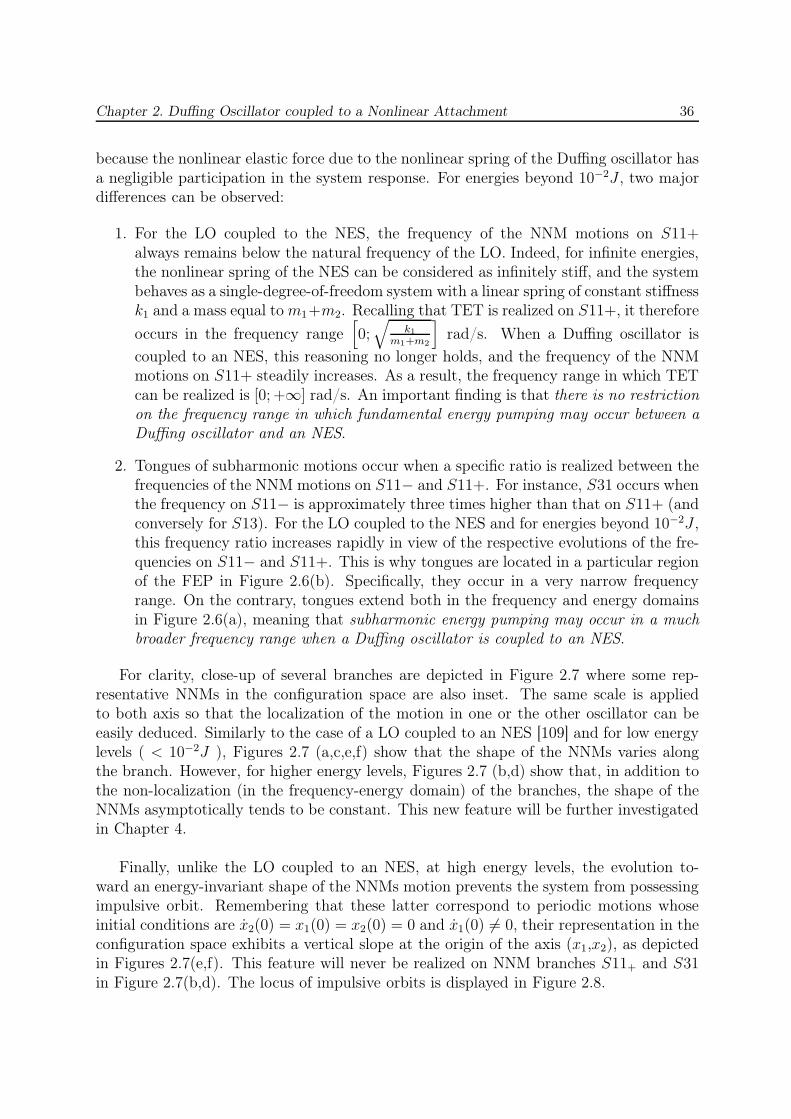
Chapter 2. Duffing Oscillator coupled to a Nonlinear Attachment 36
because the nonlinear elastic force due to the nonlinear spring of the Duffing oscillator hasa negligible participation in the system response. For energies beyond 10−2J , two majordifferences can be observed:
1. For the LO coupled to the NES, the frequency of the NNM motions on S11+always remains below the natural frequency of the LO. Indeed, for infinite energies,the nonlinear spring of the NES can be considered as infinitely stiff, and the systembehaves as a single-degree-of-freedom system with a linear spring of constant stiffnessk1 and a mass equal to m1+m2. Recalling that TET is realized on S11+, it therefore
occurs in the frequency range[
0;√
k1
m1+m2
]
rad/s. When a Duffing oscillator is
coupled to an NES, this reasoning no longer holds, and the frequency of the NNMmotions on S11+ steadily increases. As a result, the frequency range in which TETcan be realized is [0; +∞] rad/s. An important finding is that there is no restrictionon the frequency range in which fundamental energy pumping may occur between aDuffing oscillator and an NES.
2. Tongues of subharmonic motions occur when a specific ratio is realized between thefrequencies of the NNM motions on S11− and S11+. For instance, S31 occurs whenthe frequency on S11− is approximately three times higher than that on S11+ (andconversely for S13). For the LO coupled to the NES and for energies beyond 10−2J ,this frequency ratio increases rapidly in view of the respective evolutions of the fre-quencies on S11− and S11+. This is why tongues are located in a particular regionof the FEP in Figure 2.6(b). Specifically, they occur in a very narrow frequencyrange. On the contrary, tongues extend both in the frequency and energy domainsin Figure 2.6(a), meaning that subharmonic energy pumping may occur in a muchbroader frequency range when a Duffing oscillator is coupled to an NES.
For clarity, close-up of several branches are depicted in Figure 2.7 where some rep-resentative NNMs in the configuration space are also inset. The same scale is appliedto both axis so that the localization of the motion in one or the other oscillator can beeasily deduced. Similarly to the case of a LO coupled to an NES [109] and for low energylevels ( < 10−2J ), Figures 2.7 (a,c,e,f) show that the shape of the NNMs varies alongthe branch. However, for higher energy levels, Figures 2.7 (b,d) show that, in addition tothe non-localization (in the frequency-energy domain) of the branches, the shape of theNNMs asymptotically tends to be constant. This new feature will be further investigatedin Chapter 4.
Finally, unlike the LO coupled to an NES, at high energy levels, the evolution to-ward an energy-invariant shape of the NNMs motion prevents the system from possessingimpulsive orbit. Remembering that these latter correspond to periodic motions whoseinitial conditions are x2(0) = x1(0) = x2(0) = 0 and x1(0) 6= 0, their representation in theconfiguration space exhibits a vertical slope at the origin of the axis (x1,x2), as depictedin Figures 2.7(e,f). This feature will never be realized on NNM branches S11+ and S31in Figure 2.7(b,d). The locus of impulsive orbits is displayed in Figure 2.8.
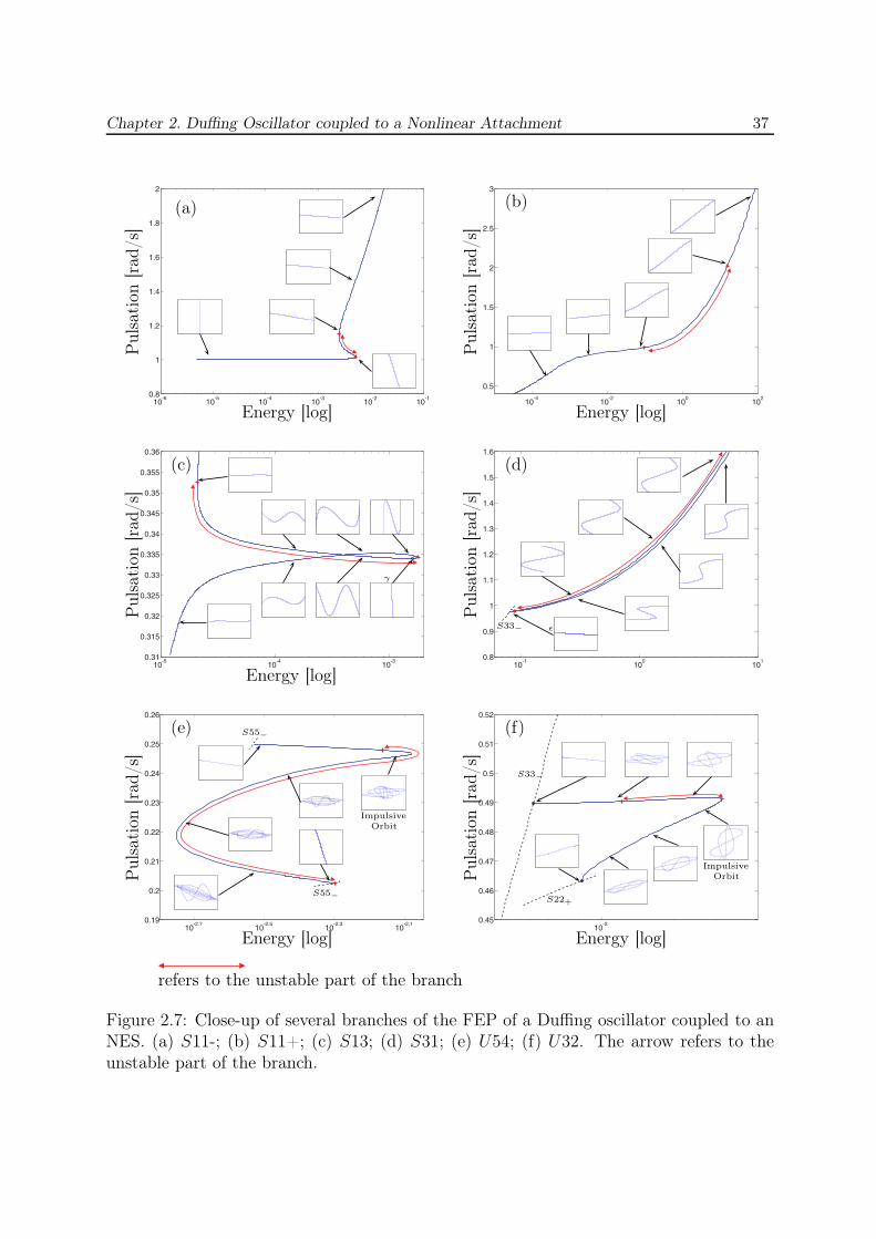
Chapter 2. Duffing Oscillator coupled to a Nonlinear Attachment 37
Energy [log]
Puls
atio
n[r
ad/s
]
(a)
Energy [log]
Puls
atio
n[r
ad/s
]
(b)
Energy [log]
Puls
atio
n[r
ad/s
]
γ
(c)P
uls
atio
n[r
ad/s
]
ǫ
(d)
S33−
Energy [log]
Puls
atio
n[r
ad/s
]
ImpulsiveOrbit
(e) S55−
S55−
Energy [log]
Puls
atio
n[r
ad/s
]
ImpulsiveOrbit
(f)
S33−
S22+
refers to the unstable part of the branch
Figure 2.7: Close-up of several branches of the FEP of a Duffing oscillator coupled to anNES. (a) S11-; (b) S11+; (c) S13; (d) S31; (e) U54; (f) U32. The arrow refers to theunstable part of the branch.
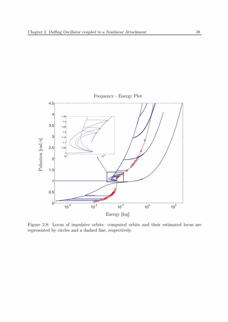
Chapter 2. Duffing Oscillator coupled to a Nonlinear Attachment 38
Puls
atio
n[r
ad/s
]
Frequency - Energy Plot
Energy [log]
Figure 2.8: Locus of impulsive orbits: computed orbits and their estimated locus arerepresented by circles and a dashed line, respectively.
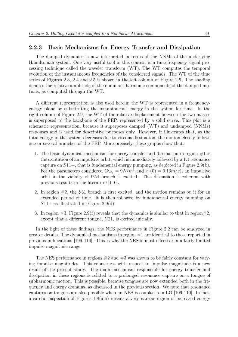
Chapter 2. Duffing Oscillator coupled to a Nonlinear Attachment 39
2.2.3 Basic Mechanisms for Energy Transfer and Dissipation
The damped dynamics is now interpreted in terms of the NNMs of the underlyingHamiltonian system. One very useful tool in this context is a time-frequency signal pro-cessing technique called the wavelet transform (WT). The WT computes the temporalevolution of the instantaneous frequencies of the considered signals. The WT of the timeseries of Figures 2.3, 2.4 and 2.5 is shown in the left column of Figure 2.9. The shadingdenotes the relative amplitude of the dominant harmonic components of the damped mo-tions, as computed through the WT.
A different representation is also used herein; the WT is represented in a frequency-energy plane by substituting the instantaneous energy in the system for time. In theright column of Figure 2.9, the WT of the relative displacement between the two massesis superposed to the backbone of the FEP, represented by a solid curve. This plot is aschematic representation, because it superposes damped (WT) and undamped (NNMs)responses and is used for descriptive purposes only. However, it illustrates that, as thetotal energy in the system decreases due to viscous dissipation, the motion closely followsone or several branches of the FEP. More precisely, these graphs show that:
1. The basic dynamical mechanism for energy transfer and dissipation in region #1 isthe excitation of an impulsive orbit, which is immediately followed by a 1:1 resonancecapture on S11+, that is fundamental energy pumping, as depicted in Figure 2.9(b).For the parameters considered (knl1 = 9N/m3 and x1(0) = 0.13m/s), an impulsiveorbit in the vicinity of U54 branch is excited. This discussion is coherent withprevious results in the literature [110].
2. In region #2, the S31 branch is first excited, and the motion remains on it for anextended period of time. It is then followed by fundamental energy pumping onS11+ as illustrated in Figure 2.9(d).
3. In region #3, Figure 2.9(f) reveals that the dynamics is similar to that in region#2,except that a different tongue, U21, is excited initially.
In the light of these findings, the NES performance in Figure 2.2 can be analyzed ingreater details. The dynamical mechanisms in region #1 are identical to those reported inprevious publications [109, 110]. This is why the NES is most effective in a fairly limitedimpulse magnitude range.
The NES performance in regions #2 and #3 was shown to be fairly constant for vary-ing impulse magnitudes. This robustness with respect to impulse magnitude is a newresult of the present study. The main mechanism responsible for energy transfer anddissipation in these regions is related to a prolonged resonance capture on a tongue ofsubharmonic motion. This is possible, because tongues are now extended both in the fre-quency and energy domains, as discussed in the previous section. We note that resonancecaptures on tongues are also possible when an NES is coupled to a LO [109,110]. In fact,a careful inspection of Figures 1.8(a,b) reveals a very narrow region of increased energy

Chapter 2. Duffing Oscillator coupled to a Nonlinear Attachment 40
0 50 100 150 200 250 300 350 400 450 5000
0.1
0.2
0.3
0.4
0.5
0 50 100 150 200 250 300 350 400 450 5000
0.1
0.2
0.3
0.4
0.5
Time [s]
Inst
ant.
freq
uen
cy[H
z] Duffing
NES
(a)
−6 −5.5 −5 −4.5 −4 −3.5 −3 −2.5 −2 −1.5 −10
0.2
0.4
0.6
0.8
1
1.2
1.4
1.6
1.8
2
Energy [log]
Puls
atio
n[r
ad/s
]
S11+
S11−
S13
U43
U54
U65
(b)
U54 1 : 1 Escape
Time [s]
Inst
ant.
freq
uen
cy[H
z] Duffing
NES
(c)
−6 −5 −4 −3 −2 −1 0 10
1
2
3
4
5
6
7
8
9
Energy [log]
Puls
atio
n[r
ad/s
]
S11+
S11−U21
S31
(d)
S31 1 : 1 Escape
Time [s]
Inst
ant.
freq
uen
cy[H
z] Duffing
NES
(e)
−6 −5 −4 −3 −2 −1 00
0.5
1
1.5
2
2.5
3
3.5
4
4.5
5
Energy [log]
Puls
atio
n[r
ad/s
]
S11+
S11−
U21
(f)
U21 1 : 1 Escape
Figure 2.9: Interpretation of the dynamical mechanisms related to high energy dissipation.Left column: WT; right column: WT superposed to the FEP. (a,b): knl1 = 9N/m3 andx1(0) = 0.13m/s (region #1); (c,d): knl1 = 1.3N/m3 and x1(0) = 7m/s (region #2);(e,f): knl1 = 2.9N/m3 and x1(0) = 1.9m/s (region #3).
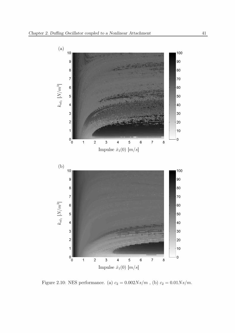
Chapter 2. Duffing Oscillator coupled to a Nonlinear Attachment 41
Impulse x1(0) [m/s]
knl 1
[N/m
3]
(a)
Impulse x1(0) [m/s]
knl 1
[N/m
3]
(b)
Figure 2.10: NES performance. (a) c2 = 0.002Ns/m , (b) c2 = 0.01Ns/m.
Chapter 2. Duffing Oscillator coupled to a Nonlinear Attachment 42
dissipation, which is located on the left of the region where the NES performs best. Inthis region, a 3:1 resonance capture is responsible for energy dissipation. However, therobustness of this dynamical mechanism is clearly questionable.
Finally, a higher NES damping coefficient c2 has been considered to assess the NESperformance under varying damping conditions. The results in Figure 2.10 demonstratethe robustness of energy dissipation in regions #1 and #2 in a fixed range of energiesx1(0) = [1; 8] [m/s]. On the contrary, energy dissipation in region #3 seems to be lessrobust, whereas regions #4 and #5 do no longer exist. From this analysis, it appears thatdamping tends to annihilate or delay the nonlinear effects to higher energy levels. Thisobservation will be further investigated in Chapters 3 and 5.
2.3 Concluding Remarks
The dynamics of a Duffing oscillator coupled to an NES was analyzed in this chapter.The dynamics of a LO coupled to an NES, reported in previous publications [90–92, 94,98, 100, 104–106, 108–110, 113, 130], and reviewed in Section 1.3.3.1, was considered as abaseline. The comparison revealed the presence of new regions of high-energy dissipation,characterized by robustness with respect to a wide range of impulse magnitudes. This isclearly an interesting finding of this chapter and paves the way for the design of nonlineardynamical absorbers which can be efficient for varying input energies.
An algorithm combining a shooting procedure with pseudo-arclength continuation wasalso introduced for the computation of a FEP. This algorithm was found to be more ro-bust and computationally efficient than that used in [109]. The combination of the FEPwith the WT showed that subharmonic energy pumping in a broad frequency range is themechanism governing the dynamics in the new regions of high-energy dissipation.
Finally, throughout this chapter, three-dimensional plots of energy dissipation werecalculated for the interpretation of the dynamics. Their computation is extremely time-consuming, and their use for NES design in real-life applications might be prohibitive.The development of a more effective design methodology is therefore required and is in-vestigated in Chapter 3.
Chapter 3
Tuning Methodology of a Nonlinear
Vibration Absorber Coupled to a
Nonlinear System : Free Vibration
Abstract
This chapter addresses the problem of mitigating the vibrations of nonlinearmechanical systems using nonlinear dynamical absorbers. One particular fea-ture of the absorber proposed in this chapter is that it is effective in a widerange of forcing amplitudes. A qualitative tuning methodology is developed andvalidated using numerical simulations. A quantitative approach targeting theassessment of an optimal functional form for the absorber is then performed.
43
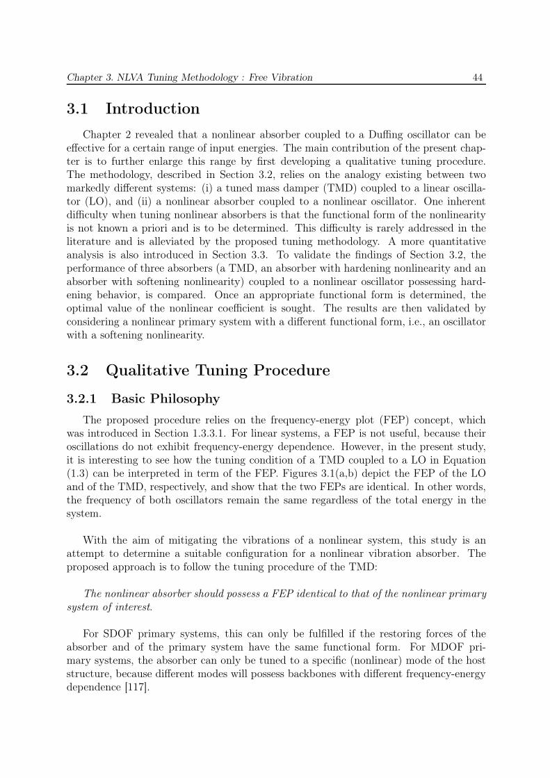
Chapter 3. NLVA Tuning Methodology : Free Vibration 44
3.1 Introduction
Chapter 2 revealed that a nonlinear absorber coupled to a Duffing oscillator can beeffective for a certain range of input energies. The main contribution of the present chap-ter is to further enlarge this range by first developing a qualitative tuning procedure.The methodology, described in Section 3.2, relies on the analogy existing between twomarkedly different systems: (i) a tuned mass damper (TMD) coupled to a linear oscilla-tor (LO), and (ii) a nonlinear absorber coupled to a nonlinear oscillator. One inherentdifficulty when tuning nonlinear absorbers is that the functional form of the nonlinearityis not known a priori and is to be determined. This difficulty is rarely addressed in theliterature and is alleviated by the proposed tuning methodology. A more quantitativeanalysis is also introduced in Section 3.3. To validate the findings of Section 3.2, theperformance of three absorbers (a TMD, an absorber with hardening nonlinearity and anabsorber with softening nonlinearity) coupled to a nonlinear oscillator possessing hard-ening behavior, is compared. Once an appropriate functional form is determined, theoptimal value of the nonlinear coefficient is sought. The results are then validated byconsidering a nonlinear primary system with a different functional form, i.e., an oscillatorwith a softening nonlinearity.
3.2 Qualitative Tuning Procedure
3.2.1 Basic Philosophy
The proposed procedure relies on the frequency-energy plot (FEP) concept, whichwas introduced in Section 1.3.3.1. For linear systems, a FEP is not useful, because theiroscillations do not exhibit frequency-energy dependence. However, in the present study,it is interesting to see how the tuning condition of a TMD coupled to a LO in Equation(1.3) can be interpreted in term of the FEP. Figures 3.1(a,b) depict the FEP of the LOand of the TMD, respectively, and show that the two FEPs are identical. In other words,the frequency of both oscillators remain the same regardless of the total energy in thesystem.
With the aim of mitigating the vibrations of a nonlinear system, this study is anattempt to determine a suitable configuration for a nonlinear vibration absorber. Theproposed approach is to follow the tuning procedure of the TMD:
The nonlinear absorber should possess a FEP identical to that of the nonlinear primarysystem of interest.
For SDOF primary systems, this can only be fulfilled if the restoring forces of theabsorber and of the primary system have the same functional form. For MDOF pri-mary systems, the absorber can only be tuned to a specific (nonlinear) mode of the hoststructure, because different modes will possess backbones with different frequency-energydependence [117].
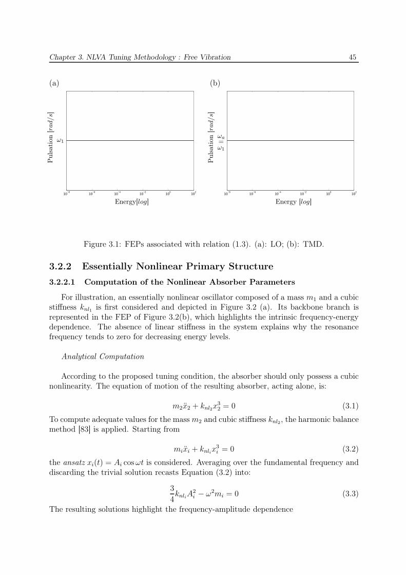
Chapter 3. NLVA Tuning Methodology : Free Vibration 45
10−8
10−6
10−4
10−2
100
102
Energy[log]
Puls
ation
[rad/s]
(a)
ω1
10−8
10−6
10−4
10−2
100
102
Energy [log]
Puls
ation
[rad/s]
ωa=ω1
(b)
Figure 3.1: FEPs associated with relation (1.3). (a): LO; (b): TMD.
3.2.2 Essentially Nonlinear Primary Structure
3.2.2.1 Computation of the Nonlinear Absorber Parameters
For illustration, an essentially nonlinear oscillator composed of a mass m1 and a cubicstiffness knl1 is first considered and depicted in Figure 3.2 (a). Its backbone branch isrepresented in the FEP of Figure 3.2(b), which highlights the intrinsic frequency-energydependence. The absence of linear stiffness in the system explains why the resonancefrequency tends to zero for decreasing energy levels.
Analytical Computation
According to the proposed tuning condition, the absorber should only possess a cubicnonlinearity. The equation of motion of the resulting absorber, acting alone, is:
m2x2 + knl2x32 = 0 (3.1)
To compute adequate values for the mass m2 and cubic stiffness knl2, the harmonic balancemethod [83] is applied. Starting from
mixi + knlix3i = 0 (3.2)
the ansatz xi(t) = Ai cos ωt is considered. Averaging over the fundamental frequency anddiscarding the trivial solution recasts Equation (3.2) into:
3
4knliA
2i − ω2mi = 0 (3.3)
The resulting solutions highlight the frequency-amplitude dependence
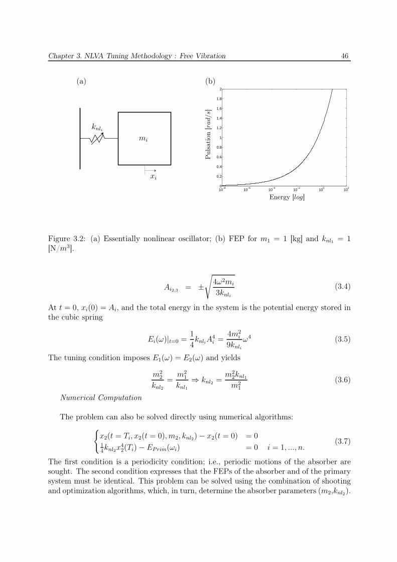
Chapter 3. NLVA Tuning Methodology : Free Vibration 46
(a)
10−8
10−6
10−4
10−2
100
1020
0.2
0.4
0.6
0.8
1
1.2
1.4
1.6
1.8
2
Energy [log]
Puls
ation
[rad/s]
(b)
knli
mi
xi
Figure 3.2: (a) Essentially nonlinear oscillator; (b) FEP for m1 = 1 [kg] and knl1 = 1[N/m3].
Ai2,3 = ±√
4ω2mi
3knli
(3.4)
At t = 0, xi(0) = Ai, and the total energy in the system is the potential energy stored inthe cubic spring
Ei(ω)|t=0 =1
4knliA
4i =
4m2i
9knli
ω4 (3.5)
The tuning condition imposes E1(ω) = E2(ω) and yields
m22
knl2
=m2
1
knl1
⇒ knl2 =m2
2knl1
m21
(3.6)
Numerical Computation
The problem can also be solved directly using numerical algorithms:
{
x2(t = Ti, x2(t = 0), m2, knl2) − x2(t = 0) = 014knl2x
42(Ti) − EPrim(ωi) = 0 i = 1, ..., n.
(3.7)
The first condition is a periodicity condition; i.e., periodic motions of the absorber aresought. The second condition expresses that the FEPs of the absorber and of the primarysystem must be identical. This problem can be solved using the combination of shootingand optimization algorithms, which, in turn, determine the absorber parameters (m2,knl2).
Chapter 3. NLVA Tuning Methodology : Free Vibration 47
knl1 knl2
c1 c2
m1 m2
x1
x2
Figure 3.3: Essentially nonlinear absorber coupled to an essentially nonlinear oscillator.
This procedure gives accurate results, but the optimization algorithm is fairly sensitiveto the initial guess (non-convex problem).
3.2.2.2 Results
The impulsive response of the resulting coupled, damped system depicted in Figure3.3 is now analyzed. The equations of motion are:
m1x1 + c1x1 + c2(x1 − x2) + knl1x31 + knl2(x1 − x2)
3 = 0,m2x2 + c2(x2 − x1) + knl2(x2 − x1)
3 = 0.(3.8)
The parameters of the primary system are m1 = 1 [kg] and knl1 = 1 [N/m3]. For obviouspractical reasons, a light-weight absorber is adopted, m2 = 0.05 [kg]. The nonlinear stiff-ness of the absorber is computed according to relation (3.6), and knl2 = 0.0025 [N/m3].Weak damping c1 = c2 = 0.002 [Ns/m] is also introduced to induce energy dissipation.
The performance of the nonlinear tuned absorber is examined by numerically integrat-ing the equations of motion (3.8). A three-dimensional plot showing the energy dissipatedin the absorber against the nonlinear stiffness knl1 and the impulse magnitude x1(0) isdisplayed in Figure 3.4. Interestingly, this figure bears a strong resemblance with Figure1.5, which corresponds to a TMD coupled to a LO. For knl1 ≈ 0.3 [N/m3] and regardlessof the value of x1(0), the tuned nonlinear absorber can dissipate a major portion of theinput energy (i.e., 95%). In addition, the region of high-energy dissipation is not local-ized to a particular value of knl1 , but it extends over the interval knl1 = [0.1−0.35] [N/m3].
These results seem to validate the proposed tuning procedure, at least qualitatively:a nonlinear absorber that can mitigate the vibrations of a nonlinear primary structurein a wide range of forcing amplitudes is obtained. The quantitative agreement is lessconvincing, because the high-energy dissipation appears around knl1 = 0.3 [N/m3] andnot around knl1 = 1 [N/m3]. If the nonlinear stiffness is fixed at a value of knl2 = 0.0075[N/m3] instead of knl2 = 0.0025 [N/m3], high-energy energy dissipation appears around
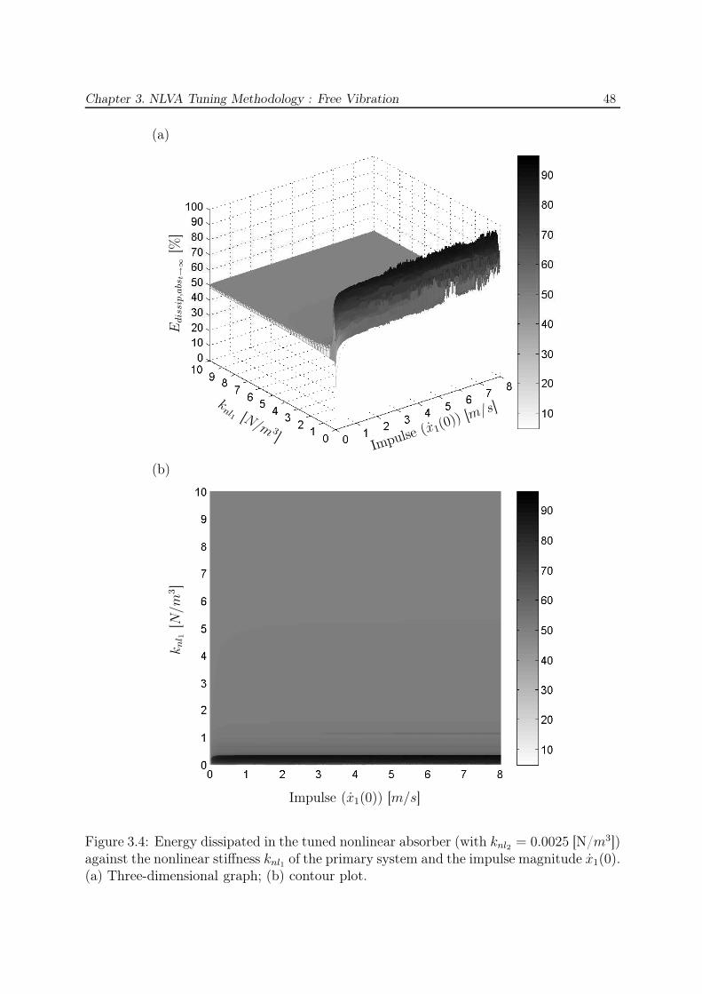
Chapter 3. NLVA Tuning Methodology : Free Vibration 48
Impulse (x1(0)) [m/s]
knl1 [N/m 3
]
Edis
sip,a
bst→
∞[%
]
(a)
Impulse (x1(0)) [m/s]
knl 1
[N/m
3]
(b)
Figure 3.4: Energy dissipated in the tuned nonlinear absorber (with knl2 = 0.0025 [N/m3])against the nonlinear stiffness knl1 of the primary system and the impulse magnitude x1(0).(a) Three-dimensional graph; (b) contour plot.

Chapter 3. NLVA Tuning Methodology : Free Vibration 49
Impulse (x1(0)) [m/s]
knl1 [N/m 3
]
Edis
sip,a
bst→
∞[%
]
(a)
Impulse (x1(0)) [m/s]
knl 1
[N/m
3]
(b)
Figure 3.5: Energy dissipated in the tuned nonlinear absorber (with knl2 = 0.0075 [N/m3])against the nonlinear stiffness (knl1) of the primary system and the impulse magnitude(x1(0)). (a) Three-dimensional graph; (b) contour plot.
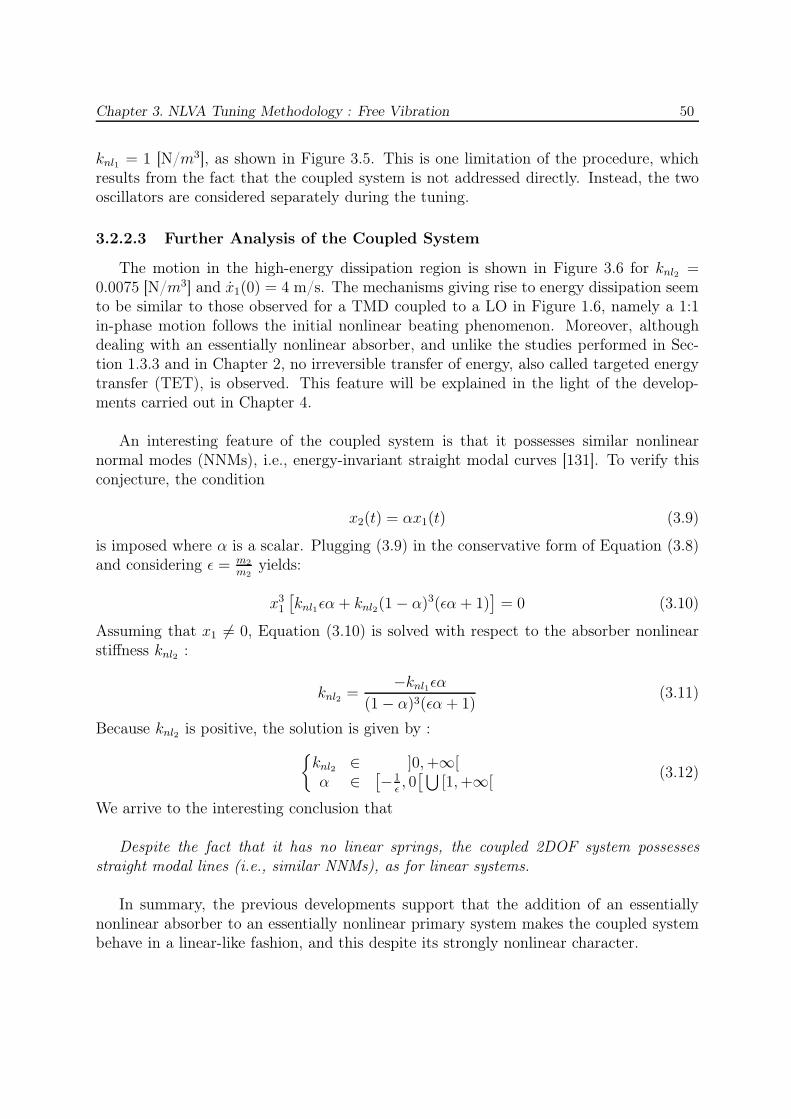
Chapter 3. NLVA Tuning Methodology : Free Vibration 50
knl1 = 1 [N/m3], as shown in Figure 3.5. This is one limitation of the procedure, whichresults from the fact that the coupled system is not addressed directly. Instead, the twooscillators are considered separately during the tuning.
3.2.2.3 Further Analysis of the Coupled System
The motion in the high-energy dissipation region is shown in Figure 3.6 for knl2 =0.0075 [N/m3] and x1(0) = 4 m/s. The mechanisms giving rise to energy dissipation seemto be similar to those observed for a TMD coupled to a LO in Figure 1.6, namely a 1:1in-phase motion follows the initial nonlinear beating phenomenon. Moreover, althoughdealing with an essentially nonlinear absorber, and unlike the studies performed in Sec-tion 1.3.3 and in Chapter 2, no irreversible transfer of energy, also called targeted energytransfer (TET), is observed. This feature will be explained in the light of the develop-ments carried out in Chapter 4.
An interesting feature of the coupled system is that it possesses similar nonlinearnormal modes (NNMs), i.e., energy-invariant straight modal curves [131]. To verify thisconjecture, the condition
x2(t) = αx1(t) (3.9)
is imposed where α is a scalar. Plugging (3.9) in the conservative form of Equation (3.8)and considering ǫ = m2
m2yields:
x31
[
knl1ǫα + knl2(1 − α)3(ǫα + 1)]
= 0 (3.10)
Assuming that x1 6= 0, Equation (3.10) is solved with respect to the absorber nonlinearstiffness knl2 :
knl2 =−knl1ǫα
(1 − α)3(ǫα + 1)(3.11)
Because knl2 is positive, the solution is given by :
{
knl2 ∈ ]0, +∞[α ∈
[
−1ǫ, 0
[⋃
[1, +∞[(3.12)
We arrive to the interesting conclusion that
Despite the fact that it has no linear springs, the coupled 2DOF system possessesstraight modal lines (i.e., similar NNMs), as for linear systems.
In summary, the previous developments support that the addition of an essentiallynonlinear absorber to an essentially nonlinear primary system makes the coupled systembehave in a linear-like fashion, and this despite its strongly nonlinear character.
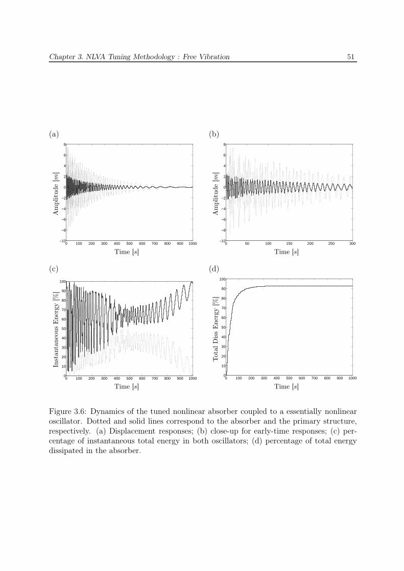
Chapter 3. NLVA Tuning Methodology : Free Vibration 51
0 100 200 300 400 500 600 700 800 900 1000−10
−8
−6
−4
−2
0
2
4
6
8
Time [s]
Am
plitu
de
[m]
(a)
0 50 100 150 200 250 300−10
−8
−6
−4
−2
0
2
4
6
8
Time [s]
Am
plitu
de
[m]
(b)
0 100 200 300 400 500 600 700 800 900 10000
10
20
30
40
50
60
70
80
90
100
Time [s]
Inst
anta
neo
us
Ener
gy
[%]
(c)
0 100 200 300 400 500 600 700 800 900 10000
10
20
30
40
50
60
70
80
90
100
Time [s]
Tota
lD
iss
Ener
gy
[%]
(d)
Figure 3.6: Dynamics of the tuned nonlinear absorber coupled to a essentially nonlinearoscillator. Dotted and solid lines correspond to the absorber and the primary structure,respectively. (a) Displacement responses; (b) close-up for early-time responses; (c) per-centage of instantaneous total energy in both oscillators; (d) percentage of total energydissipated in the absorber.
Chapter 3. NLVA Tuning Methodology : Free Vibration 52
(a)
10−4
10−3
10−2
10−1
100
101
1020
0.5
1
1.5
2
2.5
3
3.5
4
4.5
5
Energy [log]P
uls
ation
[rad/s]
(b)
knli
mi
ki
xi
Figure 3.7: Duffing oscillator. (a) Configuration; (b) FEP.
Parameter Units Valuem1 [kg] 1knl1 [N/m3] 4k1 [N/m] 1
Table 3.1: Parameters of the Duffing oscillator.
3.2.3 General Nonlinear Primary Structure
The tuning methodology of the previous section is extended to nonlinear primarysystems comprising both linear and nonlinear springs as in Figure 3.7(a). This systemmay also represents the motion of one specific nonlinear mode of a MDOF nonlinearprimary system. The frequency-energy dependence of this system is shown in the FEP ofFigure 3.7 (b) for the parameters listed in Table 3.1. At low-energy level, the dynamics isgoverned by the underlying linear system, and the oscillator exhibits a constant resonantfrequency at ω = 1 [rad/s]. For increasing energy levels, the nonlinear character of themotion becomes dominant, and the resonant frequency increases.
3.2.3.1 Computation of the Nonlinear Absorber Parameters
Analytical Computation
The equation of motion of the Duffing oscillator is
mixi + kixi + knlix3i = 0 (3.13)

Chapter 3. NLVA Tuning Methodology : Free Vibration 53
A straightforward application of the harmonic balance method gives
Ai2,3 = ±√
4(ω2mi − ki)
3knli
(3.14)
The total energy in the system is
Ei(ω)|t=0 =1
4knliA
4i +
1
2knliA
2i =
4
9knli
(
m2i ω
4 − 1
2ki(miω
2 + ki)
)
(3.15)
The tuning methodology imposes E1(ω) = E2(ω), which results in:
m21
knl1
=m2
2
knl2
,k1m1
knl1
=k2m2
knl2
, (3.16)
which can be recast into
k1
m1
=k2
m2
,m2
1
knl1
=m2
2
knl2
(3.17)
The first and second conditions are related to the tuning condition of a TMD coupled toa LO (discussed in Section 1.2) and of an essentially nonlinear absorber coupled to anessentially nonlinear oscillator (discussed in Section 3.2.2), respectively. Therefore, thetuning of the linear and nonlinear springs of the absorber can be performed by separatingexplicitly the linear and nonlinear dynamics.
Numerical Computation
The problem consists in solving the following system of equations
{
x2(t = Ti, x2(t = 0), m2, k2, knl2) − x2(t = 0) = 014knl2x
42(Ti) + 1
2k2x
22(Ti) − EPrim(ωi) = 0 i = 1, ..., n.
(3.18)
3.2.3.2 Results
The impulsive response of the coupled, damped system depicted in Figure 3.8 whoseequations of motions are :
m1x1 + c1x1 + c2(x1 − x2) + k1x1 + knl1x31 + knl2(x1 − x2)
3 + k2(x1 − x2) = 0,m2x2 + c2(x2 − x1) + k2(x2 − x1) + knl2(x2 − x1)
3 = 0.(3.19)
is now analyzed. The system parameters are given in Table 3.2 where the absorber mass issmall, and the other absorber parameters have been chosen according to Equation (3.17).Weak damping (c1 = c2 = 0.002 [Ns/m]) is also introduced in both oscillators.
A three-dimensional plot of the energy dissipated in the absorber against the nonlinearstiffness knl1 and the impulse magnitude x1(0) is numerically computed and illustrated
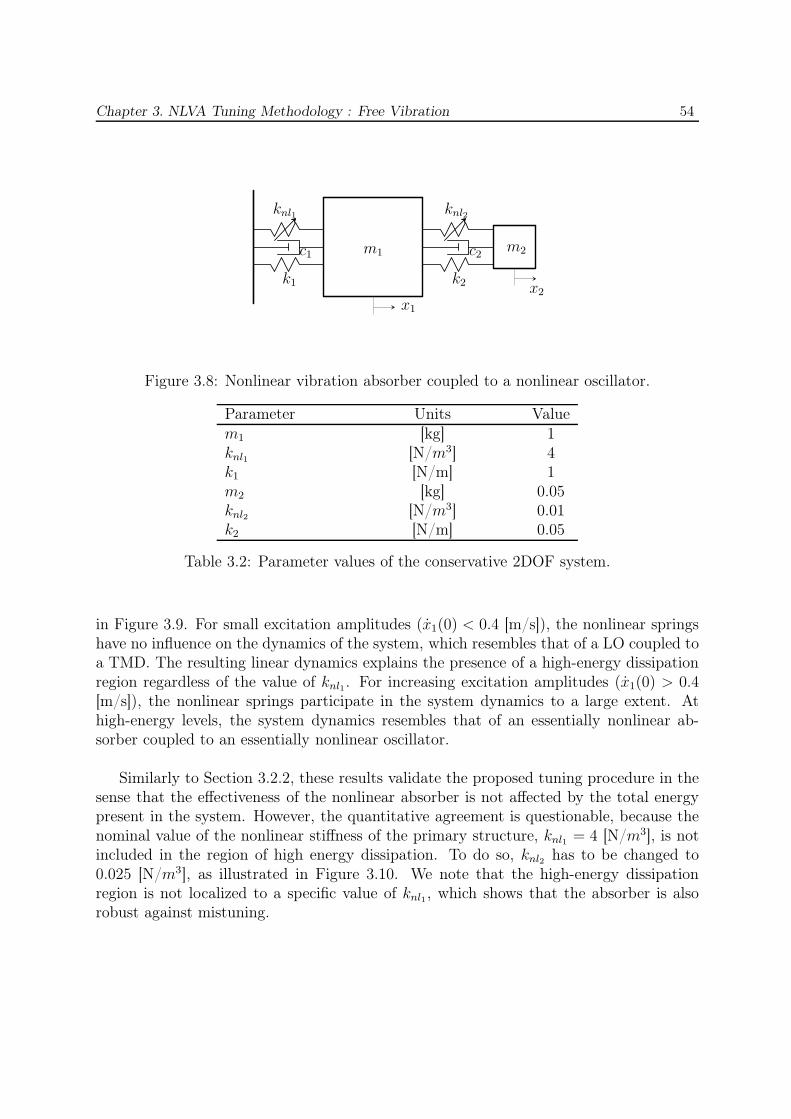
Chapter 3. NLVA Tuning Methodology : Free Vibration 54
knl1 knl2
c1 c2
k1 k2
m1 m2
x1
x2
Figure 3.8: Nonlinear vibration absorber coupled to a nonlinear oscillator.
Parameter Units Valuem1 [kg] 1knl1 [N/m3] 4k1 [N/m] 1m2 [kg] 0.05knl2 [N/m3] 0.01k2 [N/m] 0.05
Table 3.2: Parameter values of the conservative 2DOF system.
in Figure 3.9. For small excitation amplitudes (x1(0) < 0.4 [m/s]), the nonlinear springshave no influence on the dynamics of the system, which resembles that of a LO coupled toa TMD. The resulting linear dynamics explains the presence of a high-energy dissipationregion regardless of the value of knl1. For increasing excitation amplitudes (x1(0) > 0.4[m/s]), the nonlinear springs participate in the system dynamics to a large extent. Athigh-energy levels, the system dynamics resembles that of an essentially nonlinear ab-sorber coupled to an essentially nonlinear oscillator.
Similarly to Section 3.2.2, these results validate the proposed tuning procedure in thesense that the effectiveness of the nonlinear absorber is not affected by the total energypresent in the system. However, the quantitative agreement is questionable, because thenominal value of the nonlinear stiffness of the primary structure, knl1 = 4 [N/m3], is notincluded in the region of high energy dissipation. To do so, knl2 has to be changed to0.025 [N/m3], as illustrated in Figure 3.10. We note that the high-energy dissipationregion is not localized to a specific value of knl1, which shows that the absorber is alsorobust against mistuning.
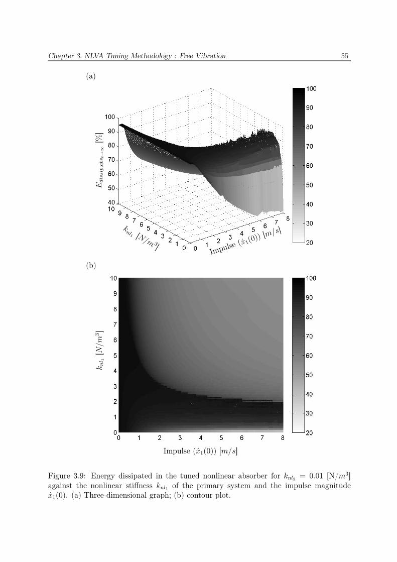
Chapter 3. NLVA Tuning Methodology : Free Vibration 55
Impulse (x1(0)) [m/s]
knl1 [N/m 3
]
Edis
sip,a
bst→
∞[%
]
(a)
Impulse (x1(0)) [m/s]
knl 1
[N/m
3]
(b)
Figure 3.9: Energy dissipated in the tuned nonlinear absorber for knl2 = 0.01 [N/m3]against the nonlinear stiffness knl1 of the primary system and the impulse magnitudex1(0). (a) Three-dimensional graph; (b) contour plot.
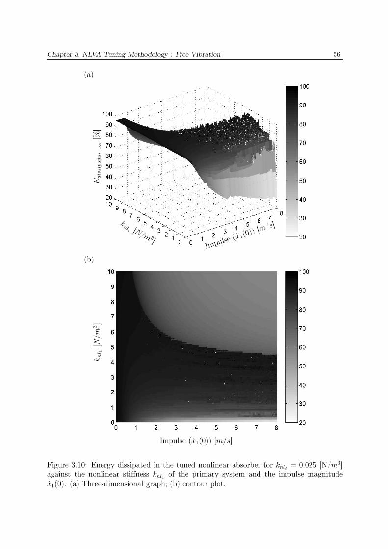
Chapter 3. NLVA Tuning Methodology : Free Vibration 56
Impulse (x1(0)) [m/s]
knl1 [N/m 3
]
Edis
sip,a
bst→
∞[%
]
(a)
Impulse (x1(0)) [m/s]
knl 1
[N/m
3]
(b)
Figure 3.10: Energy dissipated in the tuned nonlinear absorber for knl2 = 0.025 [N/m3]against the nonlinear stiffness knl1 of the primary system and the impulse magnitudex1(0). (a) Three-dimensional graph; (b) contour plot.
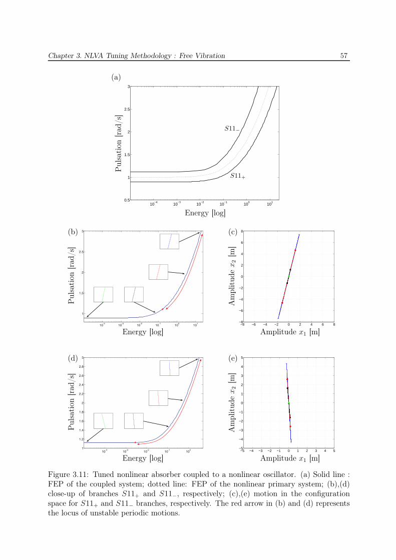
Chapter 3. NLVA Tuning Methodology : Free Vibration 57
10−4
10−3
10−2
10−1
100
101
0.5
1
1.5
2
2.5
3
S11+
S11−
Energy [log]
Puls
atio
n[r
ad/s
]
(a)
Energy [log]
Puls
atio
n[r
ad/s
]
(b)
−8 −6 −4 −2 0 2 4 6 8−8
−6
−4
−2
0
2
4
6
8
Amplitude x1 [m]
Am
plitu
de
x2
[m]
(c)
Energy [log]
Puls
atio
n[r
ad/s
]
(d)
−5 −4 −3 −2 −1 0 1 2 3 4 5−5
−4
−3
−2
−1
0
1
2
3
4
5
Amplitude x1 [m]
Am
plitu
de
x2
[m]
(e)
Figure 3.11: Tuned nonlinear absorber coupled to a nonlinear oscillator. (a) Solid line :FEP of the coupled system; dotted line: FEP of the nonlinear primary system; (b),(d)close-up of branches S11+ and S11−, respectively; (c),(e) motion in the configurationspace for S11+ and S11− branches, respectively. The red arrow in (b) and (d) representsthe locus of unstable periodic motions.
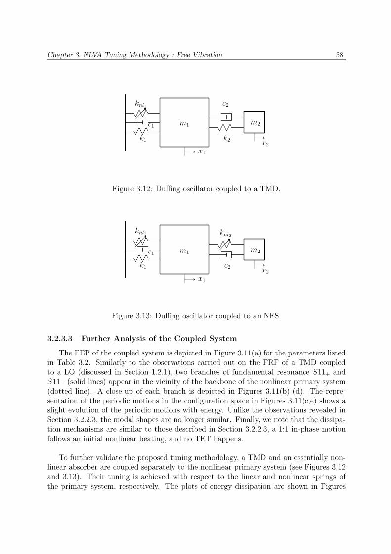
Chapter 3. NLVA Tuning Methodology : Free Vibration 58
knl1 c2
c1
k1 k2
m1 m2
x1
x2
Figure 3.12: Duffing oscillator coupled to a TMD.
knl1 knl2
c1
k1 c2
m1 m2
x1
x2
Figure 3.13: Duffing oscillator coupled to an NES.
3.2.3.3 Further Analysis of the Coupled System
The FEP of the coupled system is depicted in Figure 3.11(a) for the parameters listedin Table 3.2. Similarly to the observations carried out on the FRF of a TMD coupledto a LO (discussed in Section 1.2.1), two branches of fundamental resonance S11+ andS11− (solid lines) appear in the vicinity of the backbone of the nonlinear primary system(dotted line). A close-up of each branch is depicted in Figures 3.11(b)-(d). The repre-sentation of the periodic motions in the configuration space in Figures 3.11(c,e) shows aslight evolution of the periodic motions with energy. Unlike the observations revealed inSection 3.2.2.3, the modal shapes are no longer similar. Finally, we note that the dissipa-tion mechanisms are similar to those described in Section 3.2.2.3, a 1:1 in-phase motionfollows an initial nonlinear beating, and no TET happens.
To further validate the proposed tuning methodology, a TMD and an essentially non-linear absorber are coupled separately to the nonlinear primary system (see Figures 3.12and 3.13). Their tuning is achieved with respect to the linear and nonlinear springs ofthe primary system, respectively. The plots of energy dissipation are shown in Figures
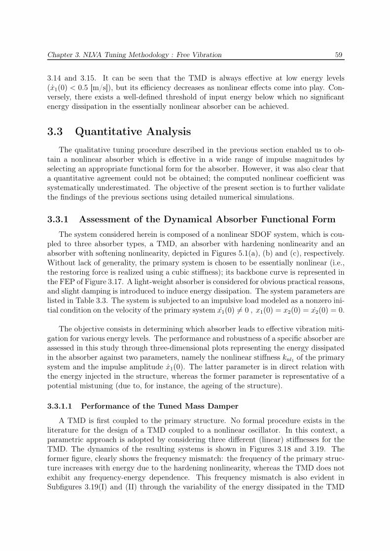
Chapter 3. NLVA Tuning Methodology : Free Vibration 59
3.14 and 3.15. It can be seen that the TMD is always effective at low energy levels(x1(0) < 0.5 [m/s]), but its efficiency decreases as nonlinear effects come into play. Con-versely, there exists a well-defined threshold of input energy below which no significantenergy dissipation in the essentially nonlinear absorber can be achieved.
3.3 Quantitative Analysis
The qualitative tuning procedure described in the previous section enabled us to ob-tain a nonlinear absorber which is effective in a wide range of impulse magnitudes byselecting an appropriate functional form for the absorber. However, it was also clear thata quantitative agreement could not be obtained; the computed nonlinear coefficient wassystematically underestimated. The objective of the present section is to further validatethe findings of the previous sections using detailed numerical simulations.
3.3.1 Assessment of the Dynamical Absorber Functional Form
The system considered herein is composed of a nonlinear SDOF system, which is cou-pled to three absorber types, a TMD, an absorber with hardening nonlinearity and anabsorber with softening nonlinearity, depicted in Figures 5.1(a), (b) and (c), respectively.Without lack of generality, the primary system is chosen to be essentially nonlinear (i.e.,the restoring force is realized using a cubic stiffness); its backbone curve is represented inthe FEP of Figure 3.17. A light-weight absorber is considered for obvious practical reasons,and slight damping is introduced to induce energy dissipation. The system parameters arelisted in Table 3.3. The system is subjected to an impulsive load modeled as a nonzero ini-tial condition on the velocity of the primary system x1(0) 6= 0 , x1(0) = x2(0) = x2(0) = 0.
The objective consists in determining which absorber leads to effective vibration miti-gation for various energy levels. The performance and robustness of a specific absorber areassessed in this study through three-dimensional plots representing the energy dissipatedin the absorber against two parameters, namely the nonlinear stiffness knl1 of the primarysystem and the impulse amplitude x1(0). The latter parameter is in direct relation withthe energy injected in the structure, whereas the former parameter is representative of apotential mistuning (due to, for instance, the ageing of the structure).
3.3.1.1 Performance of the Tuned Mass Damper
A TMD is first coupled to the primary structure. No formal procedure exists in theliterature for the design of a TMD coupled to a nonlinear oscillator. In this context, aparametric approach is adopted by considering three different (linear) stiffnesses for theTMD. The dynamics of the resulting systems is shown in Figures 3.18 and 3.19. Theformer figure, clearly shows the frequency mismatch: the frequency of the primary struc-ture increases with energy due to the hardening nonlinearity, whereas the TMD does notexhibit any frequency-energy dependence. This frequency mismatch is also evident inSubfigures 3.19(I) and (II) through the variability of the energy dissipated in the TMD
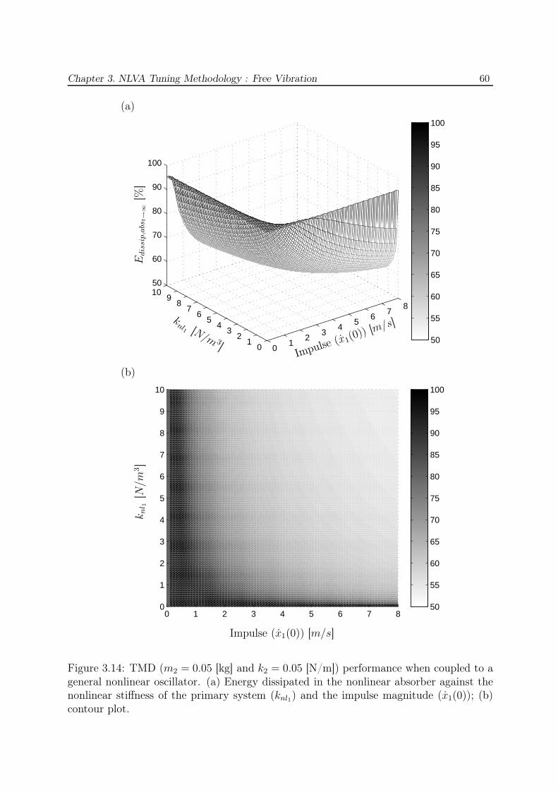
Chapter 3. NLVA Tuning Methodology : Free Vibration 60
01
23
45
67
8
01
23
45
67
89
1050
60
70
80
90
100
50
55
60
65
70
75
80
85
90
95
100
Impulse (x1(0)) [m/s]
knl1 [N/m 3
]
Edis
sip,a
bst→
∞[%
]
(a)
0 1 2 3 4 5 6 7 80
1
2
3
4
5
6
7
8
9
10
50
55
60
65
70
75
80
85
90
95
100
Impulse (x1(0)) [m/s]
knl 1
[N/m
3]
(b)
Figure 3.14: TMD (m2 = 0.05 [kg] and k2 = 0.05 [N/m]) performance when coupled to ageneral nonlinear oscillator. (a) Energy dissipated in the nonlinear absorber against thenonlinear stiffness of the primary system (knl1) and the impulse magnitude (x1(0)); (b)contour plot.
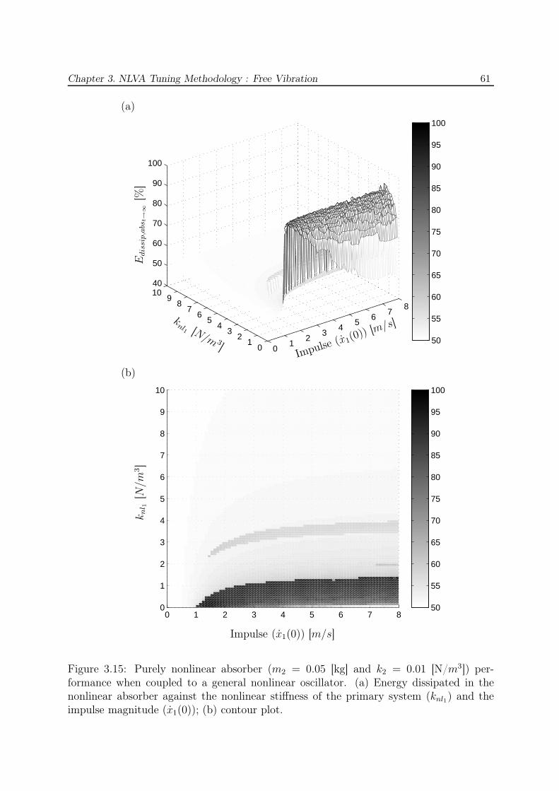
Chapter 3. NLVA Tuning Methodology : Free Vibration 61
01
23
45
67
8
01
23
45
67
89
1040
50
60
70
80
90
100
50
55
60
65
70
75
80
85
90
95
100
Impulse (x1(0)) [m/s]
knl1 [N/m 3
]
Edis
sip,a
bst→
∞[%
]
(a)
0 1 2 3 4 5 6 7 80
1
2
3
4
5
6
7
8
9
10
50
55
60
65
70
75
80
85
90
95
100
Impulse (x1(0)) [m/s]
knl 1
[N/m
3]
(b)
Figure 3.15: Purely nonlinear absorber (m2 = 0.05 [kg] and k2 = 0.01 [N/m3]) per-formance when coupled to a general nonlinear oscillator. (a) Energy dissipated in thenonlinear absorber against the nonlinear stiffness of the primary system (knl1) and theimpulse magnitude (x1(0)); (b) contour plot.
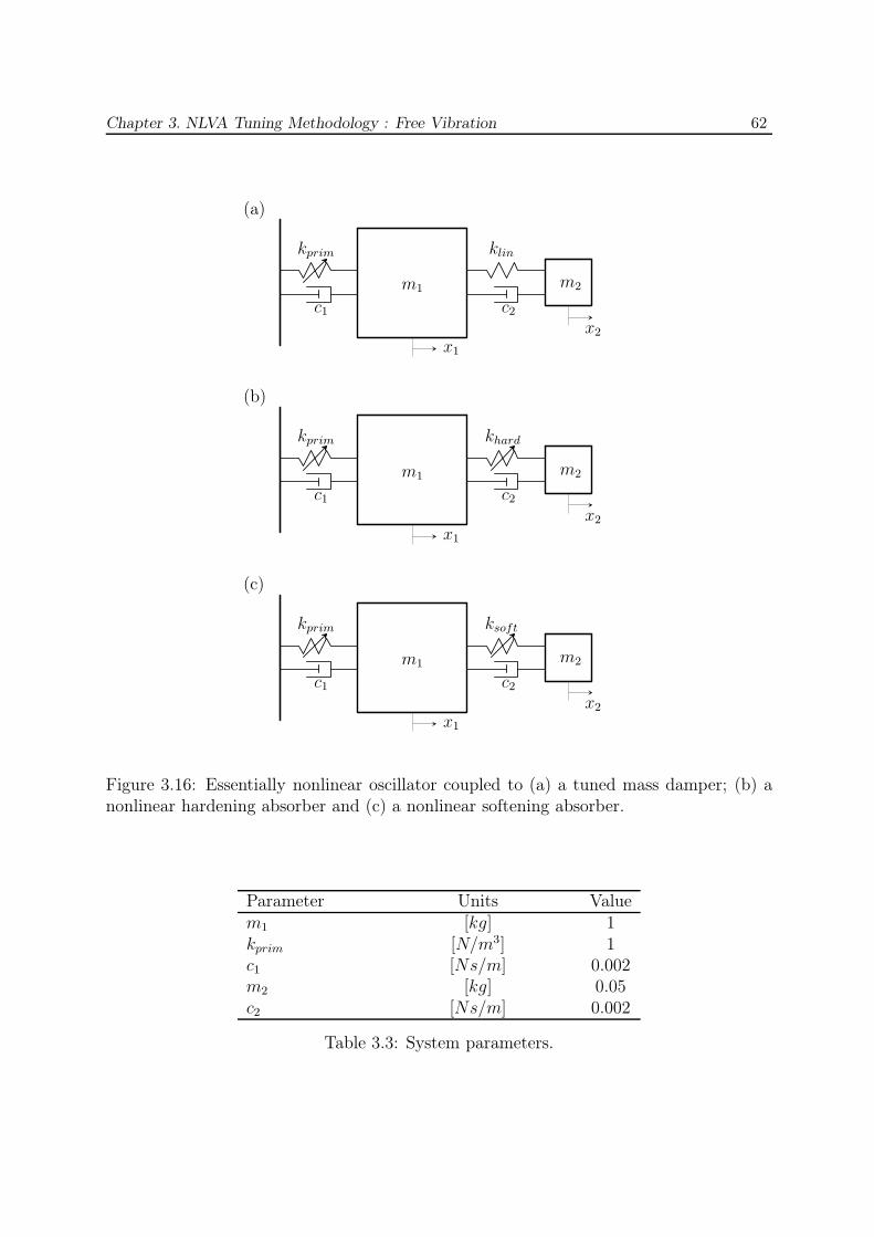
Chapter 3. NLVA Tuning Methodology : Free Vibration 62
kprim klin
c1 c2
m1 m2
x1
x2
(a)
kprim khard
c1 c2
m1 m2
x1
x2
(b)
kprim ksoft
c1 c2
m1 m2
x1
x2
(c)
Figure 3.16: Essentially nonlinear oscillator coupled to (a) a tuned mass damper; (b) anonlinear hardening absorber and (c) a nonlinear softening absorber.
Parameter Units Valuem1 [kg] 1kprim [N/m3] 1c1 [Ns/m] 0.002m2 [kg] 0.05c2 [Ns/m] 0.002
Table 3.3: System parameters.
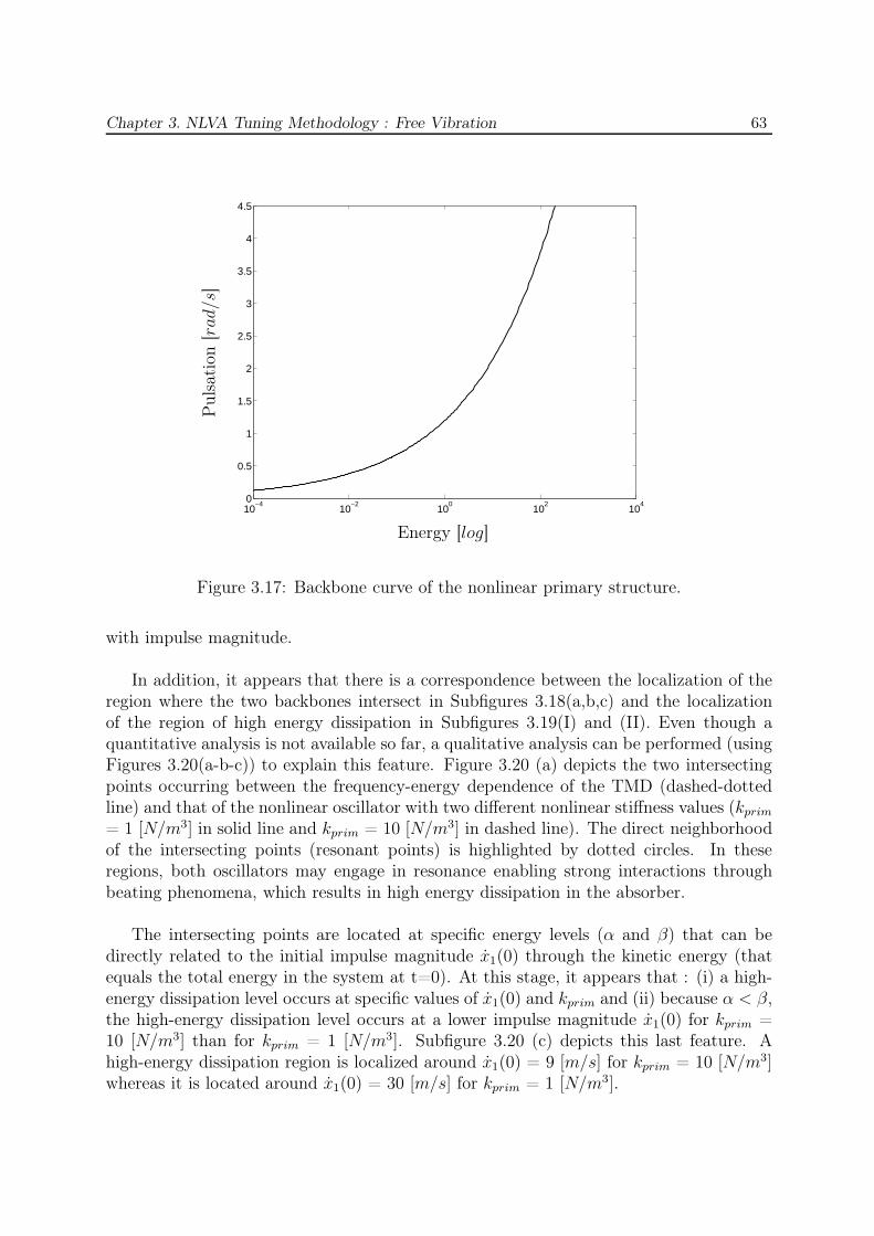
Chapter 3. NLVA Tuning Methodology : Free Vibration 63
10−4
10−2
100
102
104
0
0.5
1
1.5
2
2.5
3
3.5
4
4.5
Energy [log]
Puls
atio
n[r
ad/s
]
Figure 3.17: Backbone curve of the nonlinear primary structure.
with impulse magnitude.
In addition, it appears that there is a correspondence between the localization of theregion where the two backbones intersect in Subfigures 3.18(a,b,c) and the localizationof the region of high energy dissipation in Subfigures 3.19(I) and (II). Even though aquantitative analysis is not available so far, a qualitative analysis can be performed (usingFigures 3.20(a-b-c)) to explain this feature. Figure 3.20 (a) depicts the two intersectingpoints occurring between the frequency-energy dependence of the TMD (dashed-dottedline) and that of the nonlinear oscillator with two different nonlinear stiffness values (kprim
= 1 [N/m3] in solid line and kprim = 10 [N/m3] in dashed line). The direct neighborhoodof the intersecting points (resonant points) is highlighted by dotted circles. In theseregions, both oscillators may engage in resonance enabling strong interactions throughbeating phenomena, which results in high energy dissipation in the absorber.
The intersecting points are located at specific energy levels (α and β) that can bedirectly related to the initial impulse magnitude x1(0) through the kinetic energy (thatequals the total energy in the system at t=0). At this stage, it appears that : (i) a high-energy dissipation level occurs at specific values of x1(0) and kprim and (ii) because α < β,the high-energy dissipation level occurs at a lower impulse magnitude x1(0) for kprim =10 [N/m3] than for kprim = 1 [N/m3]. Subfigure 3.20 (c) depicts this last feature. Ahigh-energy dissipation region is localized around x1(0) = 9 [m/s] for kprim = 10 [N/m3]whereas it is located around x1(0) = 30 [m/s] for kprim = 1 [N/m3].
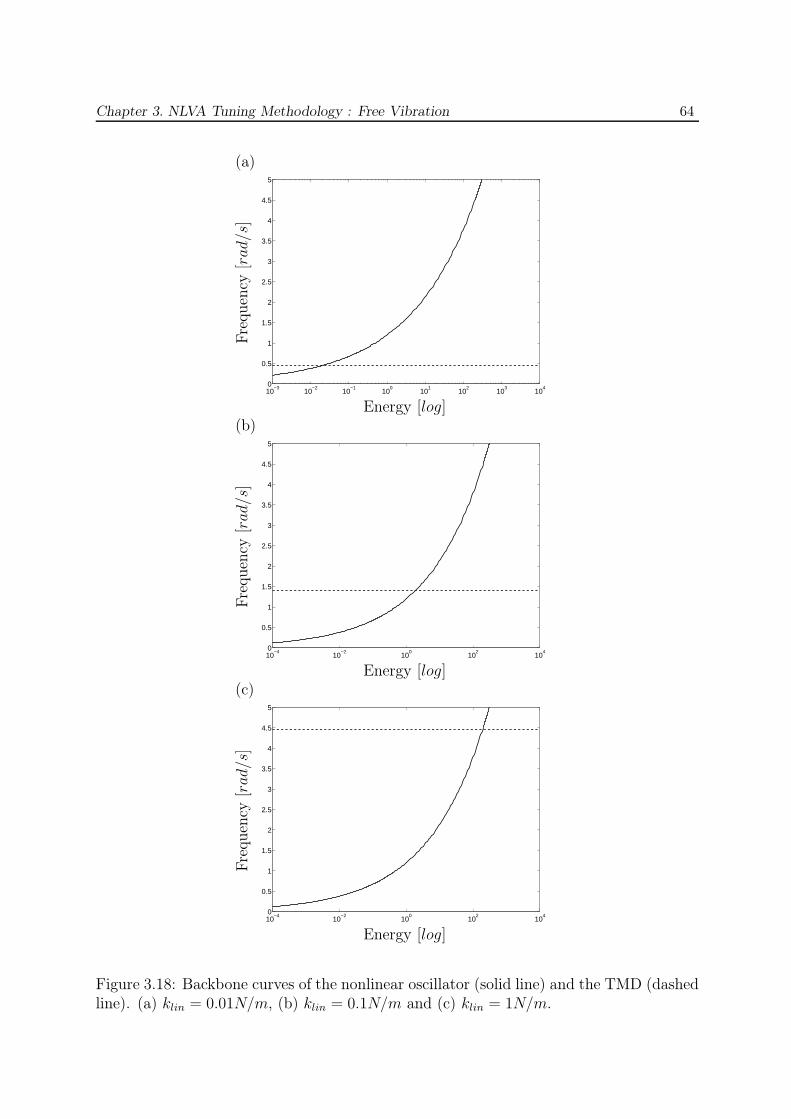
Chapter 3. NLVA Tuning Methodology : Free Vibration 64
10−3
10−2
10−1
100
101
102
103
104
0
0.5
1
1.5
2
2.5
3
3.5
4
4.5
5
10−4
10−2
100
102
104
0
0.5
1
1.5
2
2.5
3
3.5
4
4.5
5
10−4
10−2
100
102
104
0
0.5
1
1.5
2
2.5
3
3.5
4
4.5
5
(a)
(b)
(c)
Fre
quen
cy[r
ad/s
]
Energy [log]
Fre
quen
cy[r
ad/s
]
Energy [log]
Fre
quen
cy[r
ad/s
]
Energy [log]
Figure 3.18: Backbone curves of the nonlinear oscillator (solid line) and the TMD (dashedline). (a) klin = 0.01N/m, (b) klin = 0.1N/m and (c) klin = 1N/m.
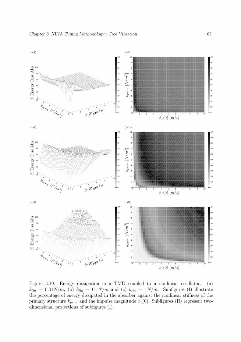
Chapter 3. NLVA Tuning Methodology : Free Vibration 65
02
46
810
0
2
4
6
8
100
20
40
60
80
100
0
10
20
30
40
50
60
70
80
90
100
02
46
810
0
2
4
6
8
100
20
40
60
80
100
0
10
20
30
40
50
60
70
80
90
100
02
46
810
0
2
4
6
8
100
20
40
60
80
100
0
10
20
30
40
50
60
70
80
90
100
0 1 2 3 4 5 6 7 8 9 100
1
2
3
4
5
6
7
8
9
10
0
10
20
30
40
50
60
70
80
90
100
0 1 2 3 4 5 6 7 8 9 100
1
2
3
4
5
6
7
8
9
10
0
10
20
30
40
50
60
70
80
90
100
0 1 2 3 4 5 6 7 8 9 100
1
2
3
4
5
6
7
8
9
10
0
10
20
30
40
50
60
70
80
90
100
(a-I) (a-II)
%E
ner
gy
Dis
sA
bs
kprim [N/m 3
] x1(0)[m/s]
kprim
[N/m
3]
x1(0) [m/s]
(b-I) (b-II)
%E
ner
gy
Dis
sA
bs
kprim [N/m 3
] x1(0)[m/s]
kprim
[N/m
3]
x1(0) [m/s]
(c-I) (c-II)
%E
ner
gy
Dis
sA
bs
kprim [N/m 3
] x1(0)[m/s]
kprim
[N/m
3]
x1(0) [m/s]
Figure 3.19: Energy dissipation in a TMD coupled to a nonlinear oscillator. (a)klin = 0.01N/m, (b) klin = 0.1N/m and (c) klin = 1N/m. Subfigures (I) illustratethe percentage of energy dissipated in the absorber against the nonlinear stiffness of theprimary structure kprim and the impulse magnitude x1(0). Subfigures (II) represent two-dimensional projections of subfigures (I).
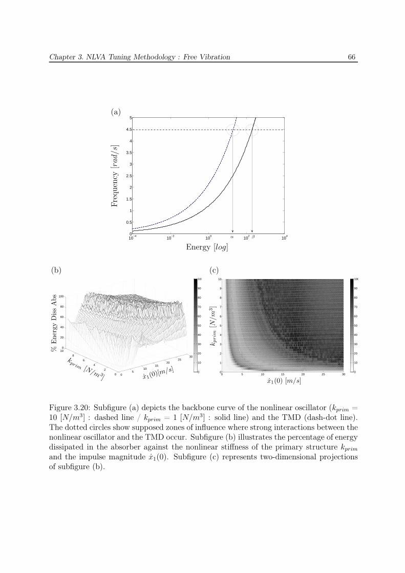
Chapter 3. NLVA Tuning Methodology : Free Vibration 66
10−4
10−2
100
102
104
0
0.5
1
1.5
2
2.5
3
3.5
4
4.5
5
05
1015
2025
30
0
2
4
6
8
100
20
40
60
80
100
0
10
20
30
40
50
60
70
80
90
100
0 5 10 15 20 25 300
1
2
3
4
5
6
7
8
9
10
0
10
20
30
40
50
60
70
80
90
100
(a)
α β
Fre
quen
cy[r
ad/s
]
Energy [log]
(b) (c)
%E
ner
gy
Dis
sA
bs
kprim [N/m 3
] x1(0)[m/s]
kprim
[N/m
3]
x1(0) [m/s]
Figure 3.20: Subfigure (a) depicts the backbone curve of the nonlinear oscillator (kprim =10 [N/m3] : dashed line / kprim = 1 [N/m3] : solid line) and the TMD (dash-dot line).The dotted circles show supposed zones of influence where strong interactions between thenonlinear oscillator and the TMD occur. Subfigure (b) illustrates the percentage of energydissipated in the absorber against the nonlinear stiffness of the primary structure kprim
and the impulse magnitude x1(0). Subfigure (c) represents two-dimensional projectionsof subfigure (b).
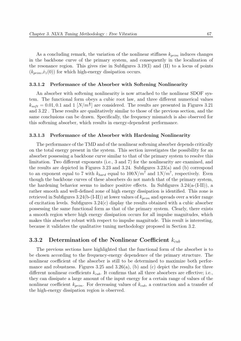
Chapter 3. NLVA Tuning Methodology : Free Vibration 67
As a concluding remark, the variation of the nonlinear stiffness kprim induces changesin the backbone curve of the primary system, and consequently in the localization ofthe resonance region. This gives rise in Subfigures 3.19(I) and (II) to a locus of points(kprim,x1(0)) for which high-energy dissipation occurs.
3.3.1.2 Performance of the Absorber with Softening Nonlinearity
An absorber with softening nonlinearity is now attached to the nonlinear SDOF sys-tem. The functional form obeys a cubic root law, and three different numerical valuesksoft = 0.01, 0.1 and 1 [N/m
13 ] are considered. The results are presented in Figures 3.21
and 3.22 . These results are qualitatively similar to those of the previous section, and thesame conclusions can be drawn. Specifically, the frequency mismatch is also observed forthis softening absorber, which results in energy-dependent performance.
3.3.1.3 Performance of the Absorber with Hardening Nonlinearity
The performance of the TMD and of the nonlinear softening absorber depends criticallyon the total energy present in the system. This section investigates the possibility for anabsorber possessing a backbone curve similar to that of the primary system to resolve thislimitation. Two different exponents (i.e., 3 and 7) for the nonlinearity are examined, andthe results are depicted in Figures 3.23 and 3.24. Subfigures 3.23(a) and (b) correspondto an exponent equal to 7 with khard equal to 100N/m7 and 1N/m7, respectively. Eventhough the backbone curves of these absorbers do not match that of the primary system,the hardening behavior seems to induce positive effects. In Subfigures 3.24(a-(I-II)), arather smooth and well-defined zone of high energy dissipation is identified. This zone isretrieved in Subfigures 3.24(b-(I-II)) at lower values of kprim and spreads over a wider rangeof excitation levels. Subfigures 3.24(c) display the results obtained with a cubic absorberpossessing the same functional form as that of the primary system. Clearly, there existsa smooth region where high energy dissipation occurs for all impulse magnitudes, whichmakes this absorber robust with respect to impulse magnitude. This result is interesting,because it validates the qualitative tuning methodology proposed in Section 3.2.
3.3.2 Determination of the Nonlinear Coefficient kcub
The previous sections have highlighted that the functional form of the absorber is tobe chosen according to the frequency-energy dependence of the primary structure. Thenonlinear coefficient of the absorber is still to be determined to maximize both perfor-mance and robustness. Figures 3.25 and 3.26(a), (b) and (c) depict the results for threedifferent nonlinear coefficients kcub. It confirms that all three absorbers are effective; i.e.,they can dissipate a large amount of the input energy for a certain range of values of thenonlinear coefficient kprim. For decreasing values of kcub, a contraction and a transfer ofthe high-energy dissipation region is observed.
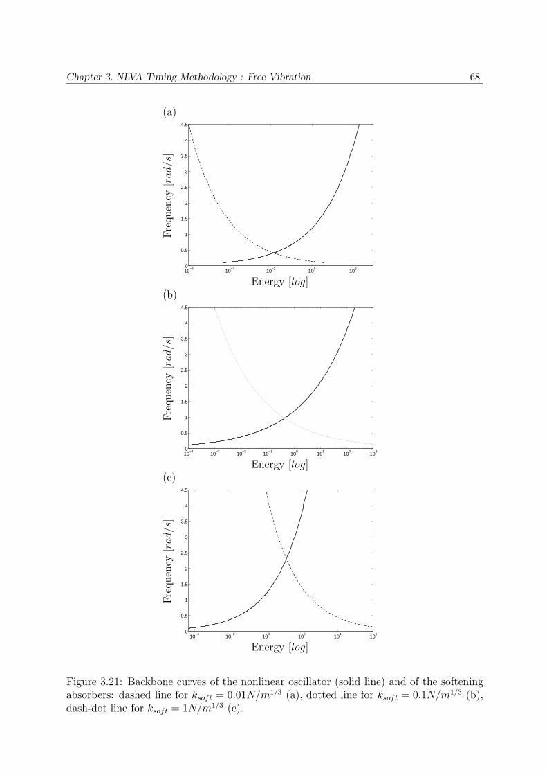
Chapter 3. NLVA Tuning Methodology : Free Vibration 68
10−6
10−4
10−2
100
102
0
0.5
1
1.5
2
2.5
3
3.5
4
4.5
10−4
10−3
10−2
10−1
100
101
102
103
0
0.5
1
1.5
2
2.5
3
3.5
4
4.5
10−4
10−2
100
102
104
106
0
0.5
1
1.5
2
2.5
3
3.5
4
4.5
(a)
(b)
(c)
Fre
quen
cy[r
ad/s
]
Energy [log]
Fre
quen
cy[r
ad/s
]
Energy [log]
Fre
quen
cy[r
ad/s
]
Energy [log]
Figure 3.21: Backbone curves of the nonlinear oscillator (solid line) and of the softeningabsorbers: dashed line for ksoft = 0.01N/m1/3 (a), dotted line for ksoft = 0.1N/m1/3 (b),dash-dot line for ksoft = 1N/m1/3 (c).

Chapter 3. NLVA Tuning Methodology : Free Vibration 69
02
46
810
0
2
4
6
8
100
20
40
60
80
100
0
10
20
30
40
50
60
70
80
90
100
02
46
810
0
2
4
6
8
100
20
40
60
80
100
0
10
20
30
40
50
60
70
80
90
100
02
46
810
0
2
4
6
8
100
20
40
60
80
100
0
10
20
30
40
50
60
70
80
90
100
0 1 2 3 4 5 6 7 8 9 100
1
2
3
4
5
6
7
8
9
10
0
10
20
30
40
50
60
70
80
90
100
0 1 2 3 4 5 6 7 8 9 100
1
2
3
4
5
6
7
8
9
10
0
10
20
30
40
50
60
70
80
90
100
0 1 2 3 4 5 6 7 8 9 100
1
2
3
4
5
6
7
8
9
10
0
10
20
30
40
50
60
70
80
90
100
(a-I) (a-II)
%E
ner
gy
Dis
sA
bs
kprim [N/m 3
] x1(0)[m/s]
kprim
[N/m
3]
x1(0) [m/s]
(b-I) (b-II)
%E
ner
gy
Dis
sA
bs
kprim [N/m 3
] x1(0)[m/s]
kprim
[N/m
3]
x1(0) [m/s]
(c-I) (c-II)
%E
ner
gy
Dis
sA
bs
kprim [N/m 3
] x1(0)[m/s]
kprim
[N/m
3]
x1(0) [m/s]
Figure 3.22: Energy dissipation in an absorber with softening nonlinearity coupled toa nonlinear oscillator. (a) ksoft = 0.01N/m1/3, (b) ksoft = 0.1N/m1/3 and (c) ksoft =1N/m1/3. Subfigures (I) illustrate the percentage of energy dissipated in the absorberagainst the nonlinear stiffness of the primary structure kprim and the impulse magnitudex1(0). Subfigures (II) represent two-dimensional projections of subfigures (I).
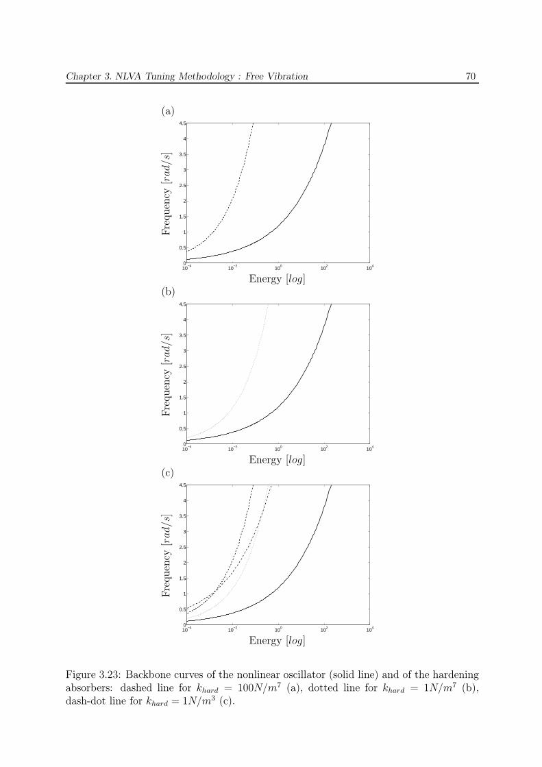
Chapter 3. NLVA Tuning Methodology : Free Vibration 70
10−4
10−2
100
102
104
0
0.5
1
1.5
2
2.5
3
3.5
4
4.5
10−4
10−2
100
102
104
0
0.5
1
1.5
2
2.5
3
3.5
4
4.5
10−4
10−2
100
102
104
0
0.5
1
1.5
2
2.5
3
3.5
4
4.5
(a)
(b)
(c)
Fre
quen
cy[r
ad/s
]
Energy [log]
Fre
quen
cy[r
ad/s
]
Energy [log]
Fre
quen
cy[r
ad/s
]
Energy [log]
Figure 3.23: Backbone curves of the nonlinear oscillator (solid line) and of the hardeningabsorbers: dashed line for khard = 100N/m7 (a), dotted line for khard = 1N/m7 (b),dash-dot line for khard = 1N/m3 (c).
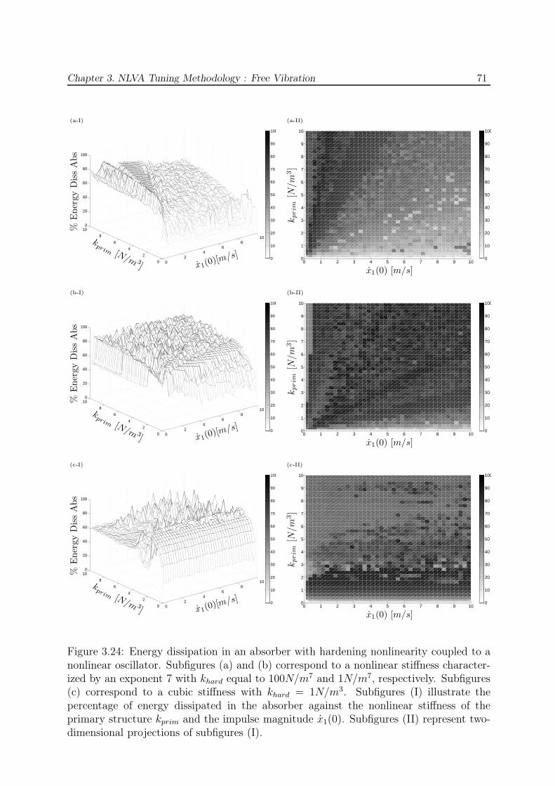
Chapter 3. NLVA Tuning Methodology : Free Vibration 71
02
46
810
0
2
4
6
8
100
20
40
60
80
100
0
10
20
30
40
50
60
70
80
90
100
02
46
810
0
2
4
6
8
100
20
40
60
80
100
0
10
20
30
40
50
60
70
80
90
100
02
46
810
0
2
4
6
8
100
20
40
60
80
100
0
10
20
30
40
50
60
70
80
90
100
0 1 2 3 4 5 6 7 8 9 100
1
2
3
4
5
6
7
8
9
10
0
10
20
30
40
50
60
70
80
90
100
0 1 2 3 4 5 6 7 8 9 100
1
2
3
4
5
6
7
8
9
10
0
10
20
30
40
50
60
70
80
90
100
0 1 2 3 4 5 6 7 8 9 100
1
2
3
4
5
6
7
8
9
10
0
10
20
30
40
50
60
70
80
90
100
(a-I) (a-II)
%E
ner
gy
Dis
sA
bs
kprim [N/m 3
] x1(0)[m/s]
kprim
[N/m
3]
x1(0) [m/s]
(b-I) (b-II)
%E
ner
gy
Dis
sA
bs
kprim [N/m 3
] x1(0)[m/s]
kprim
[N/m
3]
x1(0) [m/s]
(c-I) (c-II)
%E
ner
gy
Dis
sA
bs
kprim [N/m 3
] x1(0)[m/s]
kprim
[N/m
3]
x1(0) [m/s]
Figure 3.24: Energy dissipation in an absorber with hardening nonlinearity coupled to anonlinear oscillator. Subfigures (a) and (b) correspond to a nonlinear stiffness character-ized by an exponent 7 with khard equal to 100N/m7 and 1N/m7, respectively. Subfigures(c) correspond to a cubic stiffness with khard = 1N/m3. Subfigures (I) illustrate thepercentage of energy dissipated in the absorber against the nonlinear stiffness of theprimary structure kprim and the impulse magnitude x1(0). Subfigures (II) represent two-dimensional projections of subfigures (I).
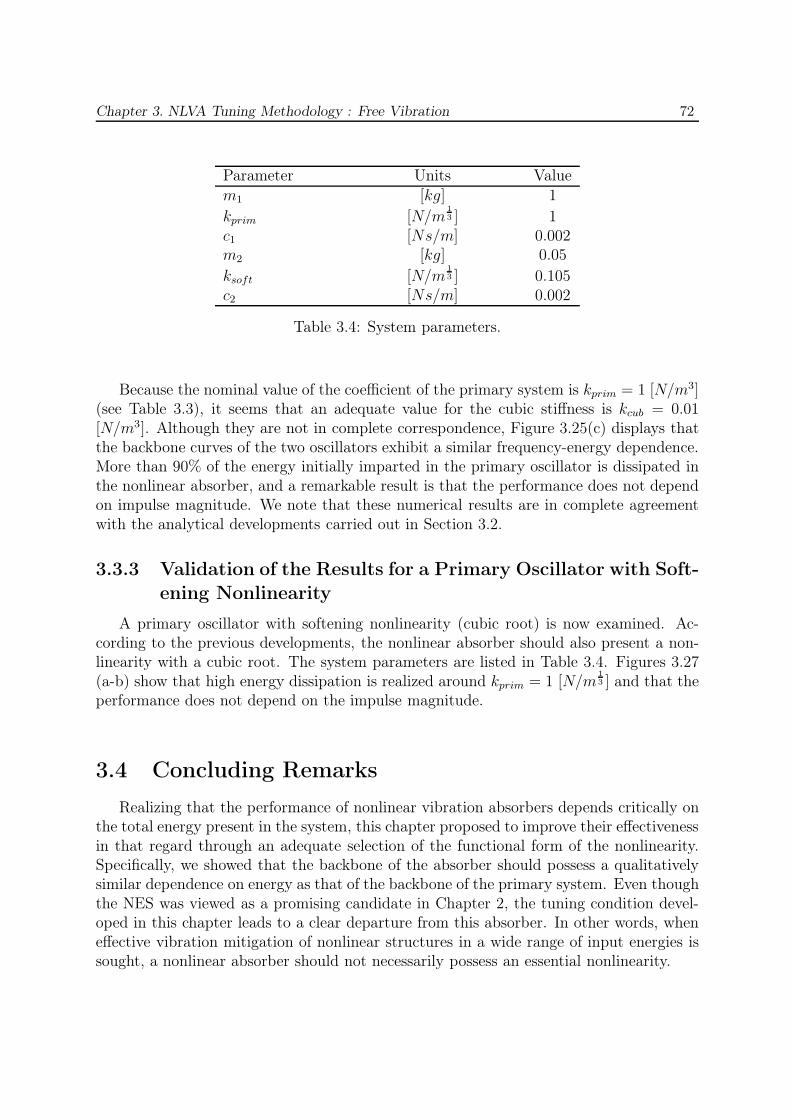
Chapter 3. NLVA Tuning Methodology : Free Vibration 72
Parameter Units Valuem1 [kg] 1
kprim [N/m13 ] 1
c1 [Ns/m] 0.002m2 [kg] 0.05
ksoft [N/m13 ] 0.105
c2 [Ns/m] 0.002
Table 3.4: System parameters.
Because the nominal value of the coefficient of the primary system is kprim = 1 [N/m3](see Table 3.3), it seems that an adequate value for the cubic stiffness is kcub = 0.01[N/m3]. Although they are not in complete correspondence, Figure 3.25(c) displays thatthe backbone curves of the two oscillators exhibit a similar frequency-energy dependence.More than 90% of the energy initially imparted in the primary oscillator is dissipated inthe nonlinear absorber, and a remarkable result is that the performance does not dependon impulse magnitude. We note that these numerical results are in complete agreementwith the analytical developments carried out in Section 3.2.
3.3.3 Validation of the Results for a Primary Oscillator with Soft-
ening Nonlinearity
A primary oscillator with softening nonlinearity (cubic root) is now examined. Ac-cording to the previous developments, the nonlinear absorber should also present a non-linearity with a cubic root. The system parameters are listed in Table 3.4. Figures 3.27(a-b) show that high energy dissipation is realized around kprim = 1 [N/m
13 ] and that the
performance does not depend on the impulse magnitude.
3.4 Concluding Remarks
Realizing that the performance of nonlinear vibration absorbers depends critically onthe total energy present in the system, this chapter proposed to improve their effectivenessin that regard through an adequate selection of the functional form of the nonlinearity.Specifically, we showed that the backbone of the absorber should possess a qualitativelysimilar dependence on energy as that of the backbone of the primary system. Even thoughthe NES was viewed as a promising candidate in Chapter 2, the tuning condition devel-oped in this chapter leads to a clear departure from this absorber. In other words, wheneffective vibration mitigation of nonlinear structures in a wide range of input energies issought, a nonlinear absorber should not necessarily possess an essential nonlinearity.
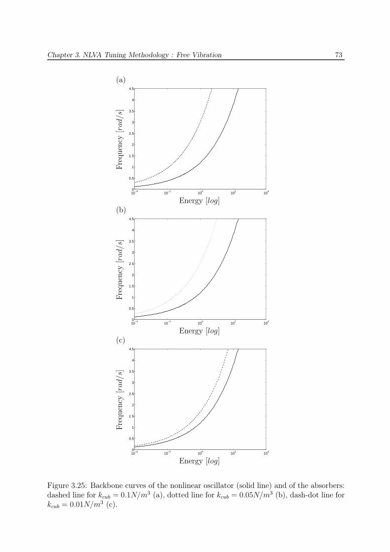
Chapter 3. NLVA Tuning Methodology : Free Vibration 73
10−4
10−2
100
102
104
0
0.5
1
1.5
2
2.5
3
3.5
4
4.5
10−4
10−2
100
102
104
0
0.5
1
1.5
2
2.5
3
3.5
4
4.5
10−4
10−2
100
102
104
0
0.5
1
1.5
2
2.5
3
3.5
4
4.5
(a)
(b)
(c)
Fre
quen
cy[r
ad/s
]
Energy [log]
Fre
quen
cy[r
ad/s
]
Energy [log]
Fre
quen
cy[r
ad/s
]
Energy [log]
Figure 3.25: Backbone curves of the nonlinear oscillator (solid line) and of the absorbers:dashed line for kcub = 0.1N/m3 (a), dotted line for kcub = 0.05N/m3 (b), dash-dot line forkcub = 0.01N/m3 (c).
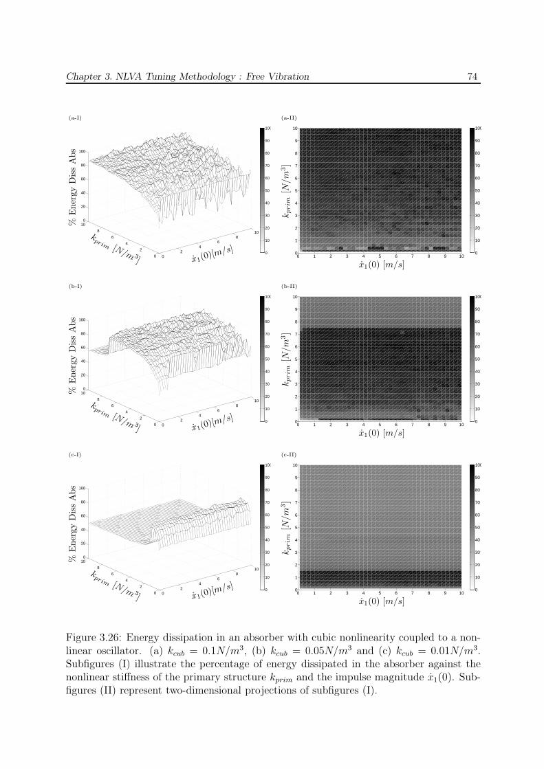
Chapter 3. NLVA Tuning Methodology : Free Vibration 74
02
46
810
0
2
4
6
8
100
20
40
60
80
100
0
10
20
30
40
50
60
70
80
90
100
02
46
810
0
2
4
6
8
100
20
40
60
80
100
0
10
20
30
40
50
60
70
80
90
100
02
46
810
0
2
4
6
8
100
20
40
60
80
100
0
10
20
30
40
50
60
70
80
90
100
0 1 2 3 4 5 6 7 8 9 100
1
2
3
4
5
6
7
8
9
10
0
10
20
30
40
50
60
70
80
90
100
0 1 2 3 4 5 6 7 8 9 100
1
2
3
4
5
6
7
8
9
10
0
10
20
30
40
50
60
70
80
90
100
0 1 2 3 4 5 6 7 8 9 100
1
2
3
4
5
6
7
8
9
10
0
10
20
30
40
50
60
70
80
90
100
(a-I) (a-II)
%E
ner
gy
Dis
sA
bs
kprim [N/m 3
] x1(0)[m/s]
kprim
[N/m
3]
x1(0) [m/s]
(b-I) (b-II)
%E
ner
gy
Dis
sA
bs
kprim [N/m 3
] x1(0)[m/s]
kprim
[N/m
3]
x1(0) [m/s]
(c-I) (c-II)
%E
ner
gy
Dis
sA
bs
kprim [N/m 3
] x1(0)[m/s]
kprim
[N/m
3]
x1(0) [m/s]
Figure 3.26: Energy dissipation in an absorber with cubic nonlinearity coupled to a non-linear oscillator. (a) kcub = 0.1N/m3, (b) kcub = 0.05N/m3 and (c) kcub = 0.01N/m3.Subfigures (I) illustrate the percentage of energy dissipated in the absorber against thenonlinear stiffness of the primary structure kprim and the impulse magnitude x1(0). Sub-figures (II) represent two-dimensional projections of subfigures (I).
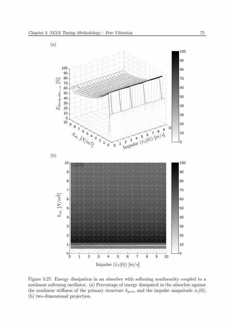
Chapter 3. NLVA Tuning Methodology : Free Vibration 75
0 1 2 3 4 5 6 7 8 9 10
01
23
45
67
89
100
102030405060708090
100
0
10
20
30
40
50
60
70
80
90
100
Impulse (x1(0)) [m/s]
knl1 [N/m 1
3 ]
Edis
sip,a
bst→
∞[%
]
(a)
0 1 2 3 4 5 6 7 8 9 100
1
2
3
4
5
6
7
8
9
10
0
10
20
30
40
50
60
70
80
90
100
Impulse (x1(0)) [m/s]
knl 1
[N/m
1 3]
(b)
Figure 3.27: Energy dissipation in an absorber with softening nonlinearity coupled to anonlinear softening oscillator. (a) Percentage of energy dissipated in the absorber againstthe nonlinear stiffness of the primary structure kprim and the impulse magnitude x1(0);(b) two-dimensional projection.
Chapter 3. NLVA Tuning Methodology : Free Vibration 76
Although these results are encouraging, several questions still need to be addressed:
1. Because the nonlinear coefficient was systematically underestimated by the method-ology described in this chapter, the next logical step is to improve the procedure sothat an accurate value for the nonlinear coefficient can be computed.
2. So far, only weak damping was introduced in the coupled system. The effects ofincreased damping are to be carefully investigated.
3. Our attention was focused on the free response of the coupled system. The consis-tency of the proposed procedure is also to be assessed in the case of forced excitation.
These issues are discussed in Chapter 5.
Finally, an interesting observation of this chapter is that, despite its strongly nonlinearcharacter, a 2DOF system comprising only essential nonlinearities possesses a linear-likebehavior. For instance, this system exhibits similar modes, i.e., energy-invariant straightmodal lines. Chapter 4 studies the dynamics of this peculiar system in more detail.
Chapter 4
Energy-Invariant Nonsimilar Nonlinear
Normal Modes in Essentially Nonlinear
Homogeneous Systems
Abstract
The present chapter analyzes the dynamical behavior of an essentially nonlineartwo-degree-of-freedom system using the nonlinear normal modes theory. Thesystem considered has a simple configuration but possesses very rich dynamics,including linear-like dynamics for some regimes of motion. In addition, thisstudy reveals the existence of energy-invariant nonsimilar nonlinear normalmodes on tongues of internal resonances.
77
Chapter 4. Energy-Invariant Nonsimilar NNMs in Essentially NL Homogeneous Systems 78
4.1 Introduction
The analysis reported in Section 2.2.2. revealed that the nonlinear normal modes(NNMs) of an essentially nonlinear attachment coupled to a Duffing oscillator tend to beenergy-invariant for increasing energies. Along the same lines, Section 3.2.2. showed thata 2DOF system comprising only essential nonlinearities may exhibit linear-like dynamicswith energy-invariant straight modal lines.
Before the present chapter analyzes this interesting dynamics more carefully, a briefreview of the NNM concept is achieved. The first definition of an NNM dates back to theseminal work carried out by Rosenberg in the 1960s [132–134] who extended the conceptof linear normal mode (LNM) to nonlinear systems. He defined an NNM as a vibration inunison of the system (i.e., a synchronous motion), which requires that all material pointsof the system reach their extreme value and pass through zero simultaneously. As pro-posed in [109,135], an extension of Rosenberg’s definition is considered herein to accountfor internally resonant NNMs; an NNM motion is therefore defined as a (non-necessarilysynchronous) periodic motion of an undamped mechanical system.
NNMs possess dynamical features that are markedly different from those of LNMsincluding frequency-energy dependence, modal interactions on branches of internal res-onances, mode bifurcations leading to a number of NNMs greater than the number ofdegrees of freedom (DOFs), the possibility to be either stable or unstable. NNMs can beclassified into two categories namely similar NNMs and nonsimilar NNMs. As discussedin [136], similar NNMs correspond to straight modal lines in configuration space and areenergy-invariant. They are not generic in nonlinear systems, because they require specialsymmetry conditions. Nonsimilar NNMs correspond to modal curves, and their shapesdepend on the total (conserved) energy present in the system. A second classification ofNNMs, as already mentioned in the introduction, can be made. Fundamental NNMs cor-respond to 1 : 1 resonant motion of the system and occur on backbone branches, whereassubharmonic NNMs imply a n : m resonant motion on tongues of internal resonances(with n 6= m).
4.2 Fundamental Dynamics of an Essentially Nonlinear
Two-Degree-of-Freedom System
The system considered herein, and depicted in Figure 4.1, is composed of two coupledessentially nonlinear oscillators. They both possess the same functional form, i.e., a cubicdependence on the displacement. The equations of motion are given by:
m1x1 + knl1x31 + knl2(x1 − x2)
3 = 0,m2x2 + knl2(x2 − x1)
3 = 0.(4.1)
and the system parameters are listed in Table 4.1.

Chapter 4. Energy-Invariant Nonsimilar NNMs in Essentially NL Homogeneous Systems 79
knl1 knl2
m1 m2
x1
x2
Figure 4.1: Essentially Nonlinear 2DOF.
Parameter Units Valuem1 [kg] 1knl1 [N/m3] 1m2 [kg] 0.05knl2 [N/m3] 0.00714
Table 4.1: Parameter values of the essentially nonlinear 2DOF system.
4.2.1 Linear-Like Dynamics
Periodic solutions of this system (i.e., NNMs) were computed numerically using analgorithm relying on a shooting procedure [129, 137]. Figure 4.2 shows some representa-tive time series. Figures 4.2(I)(a-c) depict the time series corresponding to an in-phasefundamental NNM motion (denoted S11+) and subharmonic NNM motions (1:3 internalresonance, S13, and 1:2 internal resonance, U12), respectively. Figures 4.2(II)(a-c) depictthe time series obtained when the initial conditions generating the periodic solutions (I)(a-c) are multiplied by a factor of 2. Interestingly enough, the motion amplitudes (II)(a-c)have also doubled, which reveals the occurrence of linear-like behavior for this system.Besides this feature and unlike linear systems, the frequency is also affected by the sameamplification factor.
4.2.2 Analytical Development
Based on this numerical observation, the system response to initial conditions
x1(0) = X1 x1(0) = V1
x2(0) = X2 x2(0) = V2(4.2)
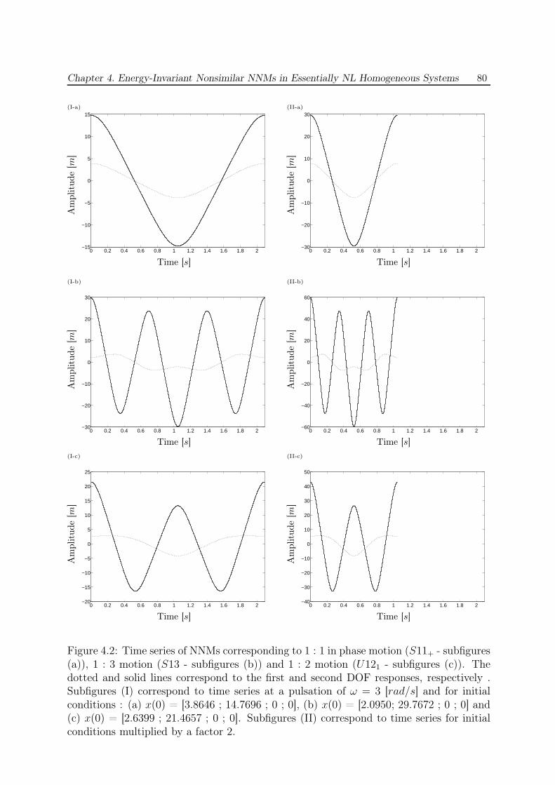
Chapter 4. Energy-Invariant Nonsimilar NNMs in Essentially NL Homogeneous Systems 80
0 0.2 0.4 0.6 0.8 1 1.2 1.4 1.6 1.8 2−15
−10
−5
0
5
10
15
Time [s]
Am
plitu
de
[m]
(I-a)
0 0.2 0.4 0.6 0.8 1 1.2 1.4 1.6 1.8 2−30
−20
−10
0
10
20
30
Time [s]
Am
plitu
de
[m]
(II-a)
0 0.2 0.4 0.6 0.8 1 1.2 1.4 1.6 1.8 2−30
−20
−10
0
10
20
30
Time [s]
Am
plitu
de
[m]
(I-b)
0 0.2 0.4 0.6 0.8 1 1.2 1.4 1.6 1.8 2−60
−40
−20
0
20
40
60
Time [s]
Am
plitu
de
[m]
(II-b)
0 0.2 0.4 0.6 0.8 1 1.2 1.4 1.6 1.8 2−20
−15
−10
−5
0
5
10
15
20
25
Time [s]
Am
plitu
de
[m]
(I-c)
0 0.2 0.4 0.6 0.8 1 1.2 1.4 1.6 1.8 2−40
−30
−20
−10
0
10
20
30
40
50
Time [s]
Am
plitu
de
[m]
(II-c)
Figure 4.2: Time series of NNMs corresponding to 1 : 1 in phase motion (S11+ - subfigures(a)), 1 : 3 motion (S13 - subfigures (b)) and 1 : 2 motion (U121 - subfigures (c)). Thedotted and solid lines correspond to the first and second DOF responses, respectively .Subfigures (I) correspond to time series at a pulsation of ω = 3 [rad/s] and for initialconditions : (a) x(0) = [3.8646 ; 14.7696 ; 0 ; 0], (b) x(0) = [2.0950; 29.7672 ; 0 ; 0] and(c) x(0) = [2.6399 ; 21.4657 ; 0 ; 0]. Subfigures (II) correspond to time series for initialconditions multiplied by a factor 2.
Chapter 4. Energy-Invariant Nonsimilar NNMs in Essentially NL Homogeneous Systems 81
is denoted xA1 (t) and xA
2 (t), respectively. On the other hand, the response to initialconditions multiplied by a factor β:
x1(0) = βX1 x1(0) = βV1
x2(0) = βX2 x2(0) = βV2(4.3)
is denoted xB1 (t) and xB
2 (t), respectively. If the linear change of variable
τ = βtx1(t) = βy1(τ)x2(t) = βy2(τ)
(4.4)
is considered, the velocity and acceleration signals become :
xi = βyi = β dyi
dτdτdt
= β2y′
i
xi = β2y′′
idτdt
= β3y′′
i
(4.5)
where apostrophe represents the differentiation with respect to the new time variable τ .The equations of motion (4.1) are transformed into:
m1y′′
1 + knl1y31 + knl2(y1 − y2)
3 = 0,m2y
′′
2 + knl2(y2 − y1)3 = 0.
(4.6)
with initial conditions (4.3) written as
y1(0) = X1 y′
1(0) = 1βV1
y2(0) = X2 y′
2(0) = 1βV2
(4.7)
If V1 = V2 = 0, the system governed by Equations (4.6) and subject to initial condi-tions (4.7) is identical to the system governed by Equations (4.1) and subject to initialconditions (4.2), which implies
y1(τ) = xA1 (t)
y2(τ) = xA2 (t)
(4.8)
Remembering the change of variable 4.4, it follows that
xB1 (t) = βxA
1 (βt)xB
2 (t) = βxA2 (βt)
(4.9)
which explains the linear-like behavior observed in Figure 4.2. Equations (4.9) expressthat the amplification of initial conditions on the displacement variables result in the sameamplification of the system response with a motion frequency increased by the same factor.
Further analytical developments were attempted to solve Equations (4.1). Refer-ence [138] shows that Jacobi elliptic functions [139] offer an exact solution of the equationof motion governing a 1DOF undamped Duffing oscillator with a linear stiffness. A num-ber of more recent studies [140–143] developed closed-form solutions for 2DOF systemswith either slight or strong nonlinearities. In the present study, the system differs from
Chapter 4. Energy-Invariant Nonsimilar NNMs in Essentially NL Homogeneous Systems 82
those previously analyzed as it is homogeneous, spatially nonsymmetric and essentiallynonlinear. Only particular solutions corresponding to 1 : 1 resonance can be found ex-plicitly with the help of elliptic functions, using ansatz described below in Section 4.2.3.2.We would prefer to obtain more general picture of possible periodic orbits and thereforehave to resort on numeric methods.
Asymptotic approaches were also considered [144,145], but the nonlinearizable natureof the system gives rise to a specific bifurcation structure (quadruple zero eigenvalue),which complicates the application of such approaches.
4.2.3 Numerical Approach
4.2.3.1 Frequency-Energy Plot
The failure of conventional analytical approaches in characterizing the dynamics of theconsidered system calls for the use of a numerical approach. This approach used hereinis based upon reference [129] and combines a shooting procedure with pseudo-arclengthcontinuation for the computation of NNMs. Eventually, the complete frequency-energydependence of NNMs can be assessed and is depicted in a FEP.
The FEP of system (4.1) is represented in Figure 4.3. A first observation is that allNNM branches arise from the origin (0; 0) of the FEP. This can be explained by the workof Gendelman et al. [146] who discussed the degeneracy of the bifurcation structure (i.e.,the existence of a pair of zero eigenfrequencies) for coupled oscillators with essential non-linearities. They demonstrated the occurrence of NNM bifurcations in the neighborhoodof stationary solutions, one of which was localized at the origin of the FEP. In our study,the absence of linear stiffness terms induces four zero eigenfrequencies, and as a result,all NNMs families bifurcate at the FEP origin.
Among the depicted branches, four of them correspond to 1 : 1 fundamental resonance,which are spread over a wide range of frequencies and energies. The other branches (i.e.,U12, S13 and S15) are associated with internally resonant NNMs [109,129]. These modalinteractions may take place between different harmonics of the fundamental NNMs, whichgenerates a countable infinity of branches of internal resonances. One interesting findingis that these branches are not localized to a particular region of the FEP, which is incontrast with previous studies performed on nonlinear systems possessing linear stiffnesscomponents [109,113,129,147]. This property also stems from the occurrence of four zeroeigenfrequencies resulting in the presence of bifurcation points at zero and infinite energylevels. A similar, but not identical, behavior was already evidenced by Tzakirtis et al.in [148] while studying the dynamics of a LO coupled to a MDOF essentially nonlinearattachment. In addition to branches of fundamental and internal resonances, an infinitenumber of singular branches consisting of subharmonic motions were identified over anextended region of the FEP. Therefore, this type of dynamical phenomena seems to berelated to the interactions occurring between essentially nonlinear oscillators.
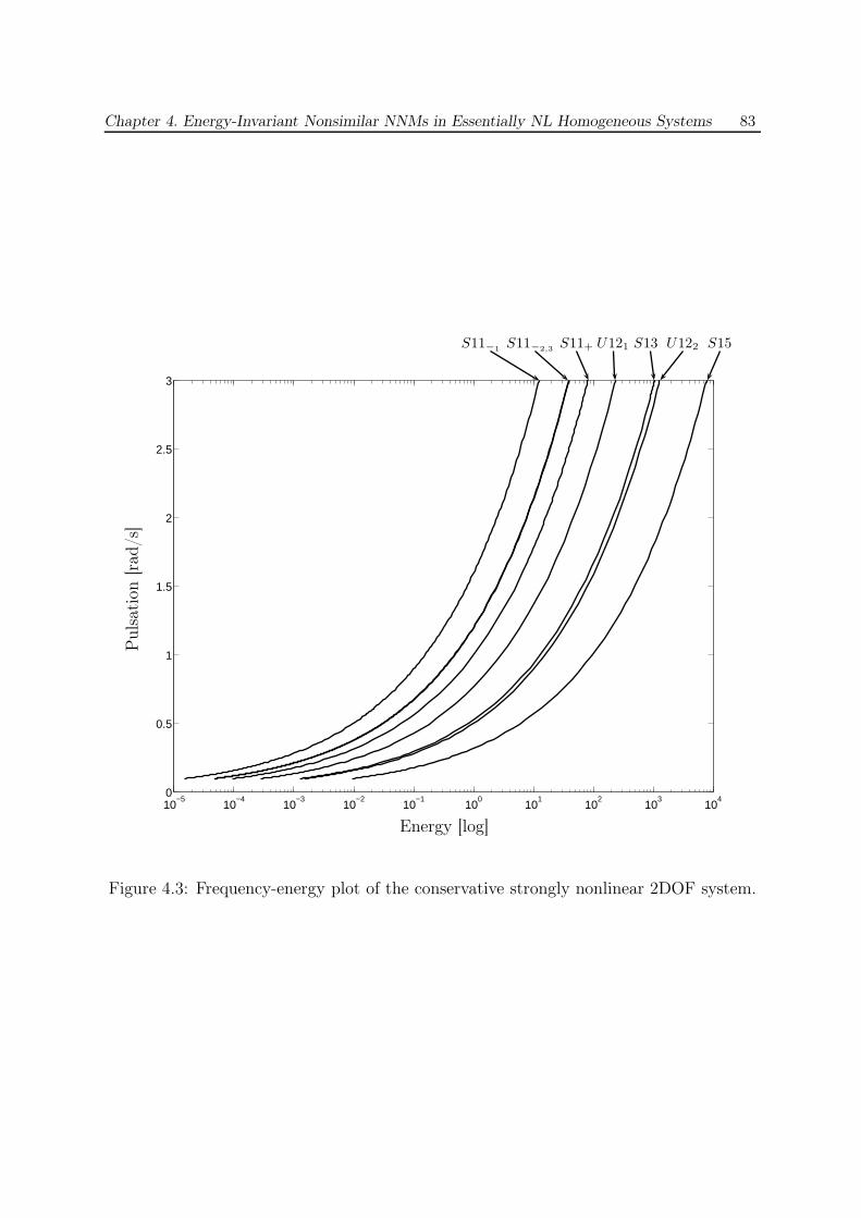
Chapter 4. Energy-Invariant Nonsimilar NNMs in Essentially NL Homogeneous Systems 83
10−5
10−4
10−3
10−2
10−1
100
101
102
103
104
0
0.5
1
1.5
2
2.5
3
S11−1
S11−2,3
S11+ U121 S13 U122 S15
Energy [log]
Puls
atio
n[r
ad/s
]
Figure 4.3: Frequency-energy plot of the conservative strongly nonlinear 2DOF system.
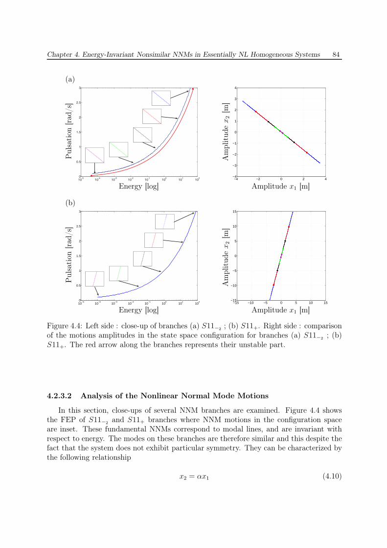
Chapter 4. Energy-Invariant Nonsimilar NNMs in Essentially NL Homogeneous Systems 84
Energy [log]
Puls
atio
n[r
ad/s
]
(a)
−4 −2 0 2 4−4
−3
−2
−1
0
1
2
3
4
Amplitude x1 [m]
Am
plitu
de
x2
[m]
10−5
10−4
10−3
10−2
10−1
100
101
102
0
0.5
1
1.5
2
2.5
3
Energy [log]
Puls
atio
n[r
ad/s
]
(b)
−15 −10 −5 0 5 10 15−15
−10
−5
0
5
10
15
Amplitude x1 [m]
Am
plitu
de
x2
[m]
Figure 4.4: Left side : close-up of branches (a) S11−2 ; (b) S11+. Right side : comparisonof the motions amplitudes in the state space configuration for branches (a) S11−2 ; (b)S11+. The red arrow along the branches represents their unstable part.
4.2.3.2 Analysis of the Nonlinear Normal Mode Motions
In this section, close-ups of several NNM branches are examined. Figure 4.4 showsthe FEP of S11−2 and S11+ branches where NNM motions in the configuration spaceare inset. These fundamental NNMs correspond to modal lines, and are invariant withrespect to energy. The modes on these branches are therefore similar and this despite thefact that the system does not exhibit particular symmetry. They can be characterized bythe following relationship
x2 = αx1 (4.10)
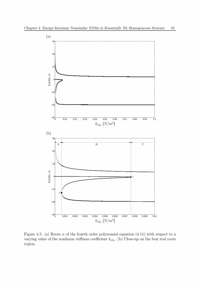
Chapter 4. Energy-Invariant Nonsimilar NNMs in Essentially NL Homogeneous Systems 85
0 0.01 0.02 0.03 0.04 0.05 0.06 0.07 0.08 0.09 0.1−30
−20
−10
0
10
20
30
knl2 [N/m3]
root
sα
(a)
0 0.001 0.002 0.003 0.004 0.005 0.006 0.007 0.008 0.009 0.01−30
−20
−10
0
10
20
30
A B C
γ
β
knl2 [N/m3]
root
sα
(b)
Figure 4.5: (a) Roots α of the fourth order polynomial equation (4.11) with respect to avarying value of the nonlinear stiffness coefficient knl2 . (b) Close-up on the four real rootsregion.
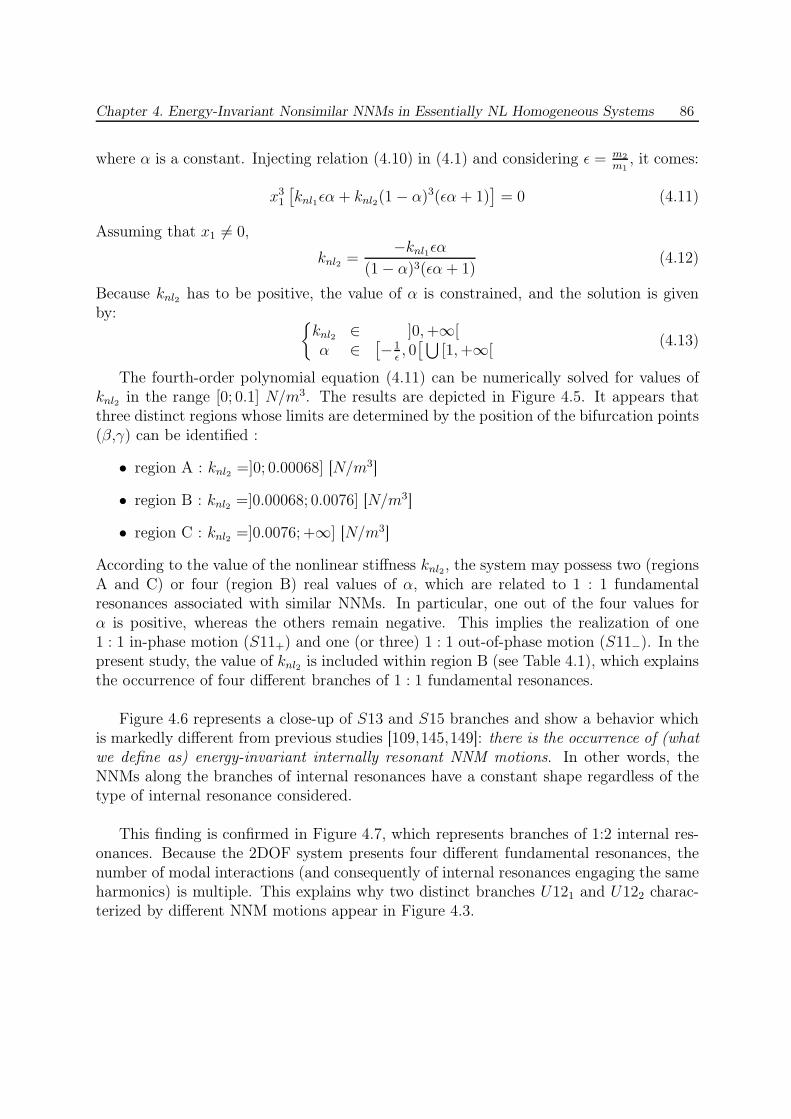
Chapter 4. Energy-Invariant Nonsimilar NNMs in Essentially NL Homogeneous Systems 86
where α is a constant. Injecting relation (4.10) in (4.1) and considering ǫ = m2
m1, it comes:
x31
[
knl1ǫα + knl2(1 − α)3(ǫα + 1)]
= 0 (4.11)
Assuming that x1 6= 0,
knl2 =−knl1ǫα
(1 − α)3(ǫα + 1)(4.12)
Because knl2 has to be positive, the value of α is constrained, and the solution is givenby:
{
knl2 ∈ ]0, +∞[α ∈
[
−1ǫ, 0
[⋃
[1, +∞[(4.13)
The fourth-order polynomial equation (4.11) can be numerically solved for values ofknl2 in the range [0; 0.1] N/m3. The results are depicted in Figure 4.5. It appears thatthree distinct regions whose limits are determined by the position of the bifurcation points(β,γ) can be identified :
• region A : knl2 =]0; 0.00068] [N/m3]
• region B : knl2 =]0.00068; 0.0076] [N/m3]
• region C : knl2 =]0.0076; +∞] [N/m3]
According to the value of the nonlinear stiffness knl2, the system may possess two (regionsA and C) or four (region B) real values of α, which are related to 1 : 1 fundamentalresonances associated with similar NNMs. In particular, one out of the four values forα is positive, whereas the others remain negative. This implies the realization of one1 : 1 in-phase motion (S11+) and one (or three) 1 : 1 out-of-phase motion (S11−). In thepresent study, the value of knl2 is included within region B (see Table 4.1), which explainsthe occurrence of four different branches of 1 : 1 fundamental resonances.
Figure 4.6 represents a close-up of S13 and S15 branches and show a behavior whichis markedly different from previous studies [109,145,149]: there is the occurrence of (whatwe define as) energy-invariant internally resonant NNM motions. In other words, theNNMs along the branches of internal resonances have a constant shape regardless of thetype of internal resonance considered.
This finding is confirmed in Figure 4.7, which represents branches of 1:2 internal res-onances. Because the 2DOF system presents four different fundamental resonances, thenumber of modal interactions (and consequently of internal resonances engaging the sameharmonics) is multiple. This explains why two distinct branches U121 and U122 charac-terized by different NNM motions appear in Figure 4.3.
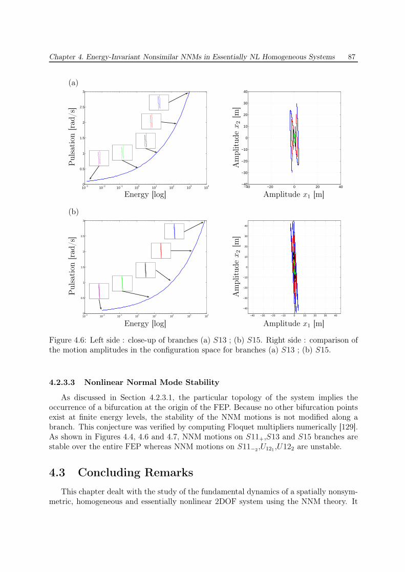
Chapter 4. Energy-Invariant Nonsimilar NNMs in Essentially NL Homogeneous Systems 87
10−3
10−2
10−1
100
101
102
103
104
0
0.5
1
1.5
2
2.5
3
Energy [log]
Puls
atio
n[r
ad/s
]
(a)
−40 −20 0 20 40−40
−30
−20
−10
0
10
20
30
40
Amplitude x1 [m]
Am
plitu
de
x2
[m]
10−3
10−2
10−1
100
101
102
103
104
0
0.5
1
1.5
2
2.5
3
Energy [log]
Puls
atio
n[r
ad/s
]
(b)
−40 −30 −20 −10 0 10 20 30 40
−40
−30
−20
−10
0
10
20
30
40
Amplitude x1 [m]
Am
plitu
de
x2
[m]
Figure 4.6: Left side : close-up of branches (a) S13 ; (b) S15. Right side : comparison ofthe motion amplitudes in the configuration space for branches (a) S13 ; (b) S15.
4.2.3.3 Nonlinear Normal Mode Stability
As discussed in Section 4.2.3.1, the particular topology of the system implies theoccurrence of a bifurcation at the origin of the FEP. Because no other bifurcation pointsexist at finite energy levels, the stability of the NNM motions is not modified along abranch. This conjecture was verified by computing Floquet multipliers numerically [129].As shown in Figures 4.4, 4.6 and 4.7, NNM motions on S11+,S13 and S15 branches arestable over the entire FEP whereas NNM motions on S11−2,U121 ,U122 are unstable.
4.3 Concluding Remarks
This chapter dealt with the study of the fundamental dynamics of a spatially nonsym-metric, homogeneous and essentially nonlinear 2DOF system using the NNM theory. It
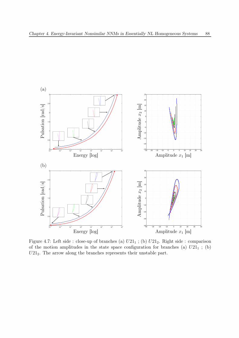
Chapter 4. Energy-Invariant Nonsimilar NNMs in Essentially NL Homogeneous Systems 88
10-4
10-3
10-2
10-1
100
101
102
103
0
0.5
1
1.5
2
2.5
3
Energy [log]
Puls
atio
n[r
ad/s
]
(a)
−25 −20 −15 −10 −5 0 5 10 15 20 25−25
−20
−15
−10
−5
0
5
10
15
20
25
Amplitude x1 [m]
Am
plitu
de
x2
[m]
10-3
10-2
10-1
100
101
102
103
104
0
0.5
1
1.5
2
2.5
3
Energy [log]
Puls
atio
n[r
ad/s
]
(b)
−40 −30 −20 −10 0 10 20 30 40−40
−30
−20
−10
0
10
20
30
40
Amplitude x1 [m]
Am
plitu
de
x2
[m]
Figure 4.7: Left side : close-up of branches (a) U211 ; (b) U212. Right side : comparisonof the motion amplitudes in the state space configuration for branches (a) U211 ; (b)U212. The arrow along the branches represents their unstable part.
Chapter 4. Energy-Invariant Nonsimilar NNMs in Essentially NL Homogeneous Systems 89
appeared that similar NNMs can be observed in such nonsymmetric systems. In addition,a new class of NNMs was highlighted, namely, energy-invariant internally resonant NNMs.It was also shown that all NNM families bifurcate out from the origin of the FEP, extendover the complete frequency-energy range and do not undergo any changes in stability.Consequently, the homogeneous and essentially nonlinear character of the system is atthe origin of a linear-like dynamical behavior for some regimes of motions observed inChapters 2 and 3. In addition to nonlinear vibration absorbers, other applications thatcould potentially benefit from the present developments are, for instance, one-dimensionalmedia composed of spherical granular beads in Hertzian contact [150]. If there is the ab-sence of pre-compression between beads, such systems will exhibit dynamics similar tothose discussed herein.
Finally, Section 3.2.2 revealed that targeted energy transfer (TET) does not occur inthe 2DOF system. Because the underlying dynamical mechanism is intimately relatedto the frequency-energy dependence of the NNMs, the absence of TET in this systemcan be directly related to the existence of energy-invariant (fundamentally and internallyresonant) NNMs.
Chapter 5
Tuning Methodology of a Nonlinear
Vibration Absorber Coupled to a
Nonlinear System : Forced Vibration
Abstract
The present chapter extends the frequency-energy-based tuning methodologyintroduced in Chapter 3 to the case of forced oscillations. The extension re-lies extensively on bifurcation analysis, and, more precisely, on the tracking ofbifurcation points in parameter space using MATCONT software. The deter-mination of accurate nonlinear coefficients for the absorber together with ap-propriate absorber damping values is also addressed. The resulting integratedtuning procedure is then presented and validated.
90
Chapter 5. NLVA Tuning Methodology : Forced Vibration 91
5.1 Introduction
The development of a tuning methodology of a nonlinear vibration absorber coupledto a nonlinear primary structure was investigated in Chapter 3 for free vibrating systems.A frequency-energy-based procedure was proposed and validated both qualitatively andquantitatively. As a result, once the frequency-energy dependence of the primary structureis known, an almost optimal configuration of the absorber can be determined. However,several improvements to the methodology still need to be brought, among which the de-termination of the nonlinear and damping coefficients of the absorber. This is the firstobjective of the present chapter. A second objective is to extend the methodology to thecase of forced oscillations.
The analysis of nonlinear systems submitted to forced excitations is performed throughthe computation of nonlinear frequency response functions (NLFRFs) for specific energylevels. The NLFRFs are characterized by a number of singularities called bifurcationpoints. In the context of nonlinear absorber tuning, these points represent relevantinformation, because they express fundamental modifications in the system dynamics.Therefore, bifurcation tracking in parameter space avoids repetitive and time-consumingcomputations of NLFRFs for varying parameters and is one important tool of this study.
The present chapter is organized as follows. Section 5.2 considers the forced responseand exploits bifurcation analysis to accurately assess the value of the absorber nonlinearstiffness and damping coefficients. The procedure is first applied to an essentially nonlinear2DOF system from which a perfectly tuned and amplitude-robust absorber arises. Basedupon these results, Section 5.3 investigates the free response of the same 2DOF systemwith the tuned absorber. The procedure is then extended to a more general nonlinearprimary structure in Section 5.4.
5.2 Bifurcation Analysis of an Essentially Nonlinear
Two-degree-of-Freedom System
5.2.1 Computation of Nonlinear Frequency Response Functions
The analysis of forced vibration is usually performed through the computation of fre-quency response functions (FRFs), which express the evolution of the motion amplitudewith excitation frequency. If their computation is straightforward for linear systems, itis more demanding in the presence of nonlinearity. As evidenced in the previous chap-ters, this dissertation relies on the extensive use of numerical techniques. Unlike analyticapproaches, computational methods are capable of (i) providing accurate solutions and(ii) dealing with strongly nonlinear regimes of motion. In this context, algorithms forthe continuation of periodic solutions are really quite sophisticated and advanced (see,e.g., AUTO [151] and MATCONT [152] software) and can be directly exploited for thecomputation of NLFRFs.
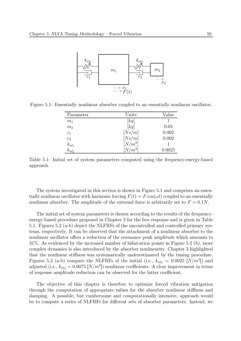
Chapter 5. NLVA Tuning Methodology : Forced Vibration 92
knl1 knl2
c1 c2
m1 m2
x1
x2
F (t)
Figure 5.1: Essentially nonlinear absorber coupled to an essentially nonlinear oscillator.
Parameter Units Valuem1 [kg] 1m2 [kg] 0.05c1 [Ns/m] 0.002c2 [Ns/m] 0.002knl1 [N/m3] 1knl2 [N/m3] 0.0025
Table 5.1: Initial set of system parameters computed using the frequency-energy-basedapproach.
The system investigated in this section is shown in Figure 5.1 and comprises an essen-tially nonlinear oscillator with harmonic forcing F (t) = F cos(ωt) coupled to an essentiallynonlinear absorber. The amplitude of the external force is arbitrarily set to F = 0.1N .
The initial set of system parameters is chosen according to the results of the frequency-energy-based procedure proposed in Chapter 3 for the free response and is given in Table5.1. Figures 5.2 (a-b) depict the NLFRFs of the uncontrolled and controlled primary sys-tems, respectively. It can be observed that the attachment of a nonlinear absorber to thenonlinear oscillator offers a reduction of the resonance peak amplitude which amounts to31%. As evidenced by the increased number of bifurcation points in Figure 5.2 (b), morecomplex dynamics is also introduced by the absorber nonlinearity. Chapter 3 highlightedthat the nonlinear stiffness was systematically underestimated by the tuning procedure.Figures 5.3 (a-b) compare the NLFRFs of the initial (i.e., knl2 = 0.0025 [N/m3]) andadjusted (i.e., knl2 = 0.0075 [N/m3]) nonlinear coefficients. A clear improvement in termsof response amplitude reduction can be observed for the latter coefficient.
The objective of this chapter is therefore to optimize forced vibration mitigationthrough the computation of appropriate values for the absorber nonlinear stiffness anddamping. A possible, but cumbersome and computationally intensive, approach wouldbe to compute a series of NLFRFs for different sets of absorber parameters. Instead, we
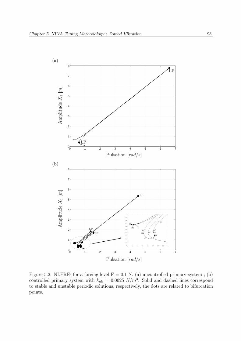
Chapter 5. NLVA Tuning Methodology : Forced Vibration 93
0 1 2 3 4 5 6 70
1
2
3
4
5
6
7
8
LP
LP
0 1 2 3 4 5 6 70
1
2
3
4
5
6
7
8
LP
LP
LP
0.2 0.3 0.4 0.5 0.6 0.7 0.8 0.9 10
0.1
0.2
0.3
0.4
0.5
0.6
0.7
0.8
0.9
1
LP
LP
LP
NS
NS
NS
PDNS
NS
LPLP
Pulsation [rad/s]
Am
plitu
de
X1
[m]
(a)
Pulsation [rad/s]
Am
plitu
de
X1
[m]
(b)
Figure 5.2: NLFRFs for a forcing level F = 0.1 N. (a) uncontrolled primary system ; (b)controlled primary system with knl2 = 0.0025 N/m3. Solid and dashed lines correspondto stable and unstable periodic solutions, respectively, the dots are related to bifurcationpoints.
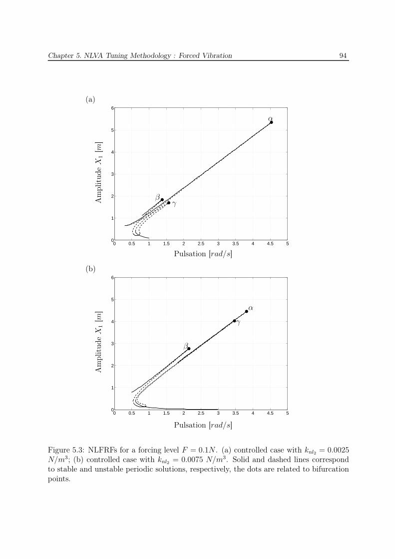
Chapter 5. NLVA Tuning Methodology : Forced Vibration 94
0 0.5 1 1.5 2 2.5 3 3.5 4 4.5 50
1
2
3
4
5
6
0 0.5 1 1.5 2 2.5 3 3.5 4 4.5 50
1
2
3
4
5
6
Pulsation [rad/s]
Am
plitu
de
X1
[m]
(a)
Pulsation [rad/s]
Am
plitu
de
X1
[m]
(b)
βγ
α
β
γ
α
Figure 5.3: NLFRFs for a forcing level F = 0.1N . (a) controlled case with knl2 = 0.0025N/m3; (b) controlled case with knl2 = 0.0075 N/m3. Solid and dashed lines correspondto stable and unstable periodic solutions, respectively, the dots are related to bifurcationpoints.
Chapter 5. NLVA Tuning Methodology : Forced Vibration 95
propose to track in parameter space the evolution of bifurcation points of NLFRFs (e.g.,α, β and γ in Figure 5.3), which contain key information about the dynamics. This isperformed next using MATCONT software.
5.2.2 Optimization of the Nonlinear Absorber Parameters
Even though a complete description of bifurcations is beyond the scope of this disser-tation (see, e.g., [153,154] for a more complete treatment), the existence of three familiesof bifurcation points in Figures 5.2 and 5.3 can be pointed out:
1. For a limit point (LP) : a pair of Floquet multipliers leaves the unit circle alongthe real axis through +1. A LP bifurcation generally indicates coexisting periodicsolutions.
2. For a Neimarck-Sacker (NS) bifurcation, a pair of Floquet multipliers leaves theunit circle in the complex plane. A NS bifurcation generally indicates coexistingquasi-periodic solutions.
3. For a period doubling (PD) bifurcation, a pair of Floquet multipliers leaves the unitcircle along the real axis through -1. A PD bifurcation may indicate the existenceof chaotic solutions.
The point of maximum amplitude of the primary structure, denoted α in Figure 5.3,corresponds to a LP bifurcation. Points β and γ corresponding to the maximum of sec-ondary resonance peaks are also LP bifurcations. These points are associated with 1:1fundamental resonances of the coupled system. Tracking the evolution of these bifur-cations for varying absorber parameters knl2 and c2 therefore enables to optimize theeffectiveness of the nonlinear absorber through the reduction of resonance peak ampli-tudes. As for the classical TMD, a possible tuning condition is to determine the absorberparameters which minimize the maximum amplitude magnification of the primary system.
However, because the excitation frequency is also a necessary parameter during nu-merical continuation, a codimension three continuation problem is to be solved, which isbeyond the current capability of MATCONT. The proposed solution is to first optimizethe absorber performance with respect to the nonlinear stiffness, which is a codimensiontwo problem. The same procedure can then be carried out for damping, and the wholeprocess can be repeated until convergence is reached.
5.2.2.1 Continuation of Limit Point Bifurcations versus (knl2,ω)
The continuation of bifurcations α, β and γ of Figure 5.3(a) with respect to nonlinearstiffness knl2 and pulsation ω is shown in Figure 5.4. Figure 5.4(a) shows the three-dimensional space whereas two-dimensional projections are depicted in Figures 5.4(b,c).
The first interesting feature is that there exists a value of the nonlinear coefficient,knl2 = 0.007601 N/m3, above which the bifurcation point γ is eliminated. At point R1,
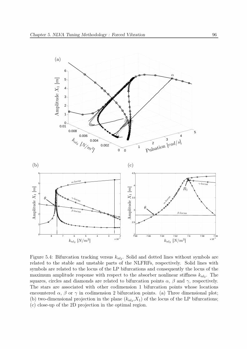
Chapter 5. NLVA Tuning Methodology : Forced Vibration 96
01
23
45
00.002
0.0040.006
0.0080.01
0
1
2
3
4
5
6
Pulsation [rad/
s]knl2 [N/m 3
]
Am
plitu
de
X1
[m]
(a)
β γ
α
2345678
x 10−3
0
1
2
3
4
5
6
knl2 [N/m3]
Am
plitu
de
X1
[m]
θ
(b)
7.567.587.67.627.647.667.68
x 10−3
2
2.5
3
3.5
4
4.5
knl2 [N/m3]
Am
plitu
de
X1
[m]
θ
(c)
R1
α-locus
β-locus
γ-locus
α-loc
us
β-locus
γ-locus
Figure 5.4: Bifurcation tracking versus knl2. Solid and dotted lines without symbols arerelated to the stable and unstable parts of the NLFRFs, respectively. Solid lines withsymbols are related to the locus of the LP bifurcations and consequently the locus of themaximum amplitude response with respect to the absorber nonlinear stiffness knl2 . Thesquares, circles and diamonds are related to bifurcation points α, β and γ, respectively.The stars are associated with other codimension 1 bifurcation points whose locationsencountered α, β or γ in codimension 2 bifurcation points. (a) Three dimensional plot;(b) two-dimensional projection in the plane (knl2,X1) of the locus of the LP bifurcations;(c) close-up of the 2D projection in the optimal region.
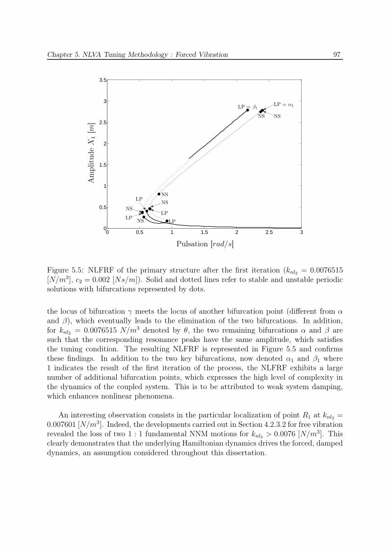
Chapter 5. NLVA Tuning Methodology : Forced Vibration 97
0 0.5 1 1.5 2 2.5 30
0.5
1
1.5
2
2.5
3
3.5
NS
LP
NS
LP = β1
LP = α1
NS
NS
LPLP
NS
LP
NS
Pulsation [rad/s]
Am
plitu
de
X1
[m]
Figure 5.5: NLFRF of the primary structure after the first iteration (knl2 = 0.0076515[N/m3], c2 = 0.002 [Ns/m]). Solid and dotted lines refer to stable and unstable periodicsolutions with bifurcations represented by dots.
the locus of bifurcation γ meets the locus of another bifurcation point (different from αand β), which eventually leads to the elimination of the two bifurcations. In addition,for knl2 = 0.0076515 N/m3 denoted by θ, the two remaining bifurcations α and β aresuch that the corresponding resonance peaks have the same amplitude, which satisfiesthe tuning condition. The resulting NLFRF is represented in Figure 5.5 and confirmsthese findings. In addition to the two key bifurcations, now denoted α1 and β1 where1 indicates the result of the first iteration of the process, the NLFRF exhibits a largenumber of additional bifurcation points, which expresses the high level of complexity inthe dynamics of the coupled system. This is to be attributed to weak system damping,which enhances nonlinear phenomena.
An interesting observation consists in the particular localization of point R1 at knl2 =0.007601 [N/m3]. Indeed, the developments carried out in Section 4.2.3.2 for free vibrationrevealed the loss of two 1 : 1 fundamental NNM motions for knl2 > 0.0076 [N/m3]. Thisclearly demonstrates that the underlying Hamiltonian dynamics drives the forced, dampeddynamics, an assumption considered throughout this dissertation.
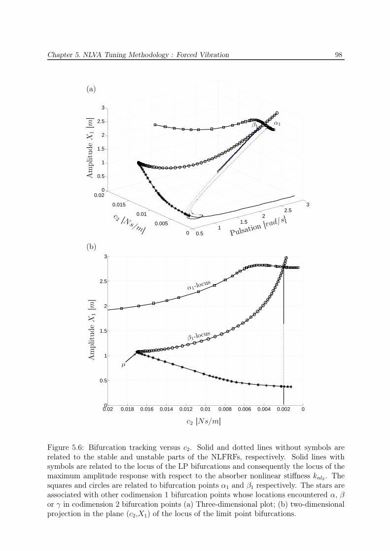
Chapter 5. NLVA Tuning Methodology : Forced Vibration 98
0.51
1.52
2.53
0
0.005
0.01
0.015
0.020
0.5
1
1.5
2
2.5
3
Pulsation [rad/
s]c2 [Ns/m]
Am
plitu
de
X1
[m]
(a)
00.0020.0040.0060.0080.010.0120.0140.0160.0180.020
0.5
1
1.5
2
2.5
3
c2 [Ns/m]
Am
plitu
de
X1
[m]
µ
(b)
β1α1
α1-locus
β1-locus
Figure 5.6: Bifurcation tracking versus c2. Solid and dotted lines without symbols arerelated to the stable and unstable parts of the NLFRFs, respectively. Solid lines withsymbols are related to the locus of the LP bifurcations and consequently the locus of themaximum amplitude response with respect to the absorber nonlinear stiffness knl2 . Thesquares and circles are related to bifurcation points α1 and β1 respectively. The stars areassociated with other codimension 1 bifurcation points whose locations encountered α, βor γ in codimension 2 bifurcation points (a) Three-dimensional plot; (b) two-dimensionalprojection in the plane (c2,X1) of the locus of the limit point bifurcations.

Chapter 5. NLVA Tuning Methodology : Forced Vibration 99
Iteration Variable knl2 c2 % of X1 reduction0 / 0.0025 0.002 311 knl2 0.0076515 0.002 652 c2 0.0076515 0.016973 743 knl2 0.01025 0.016973 85
Table 5.2: Iterative procedure for knl2 and c2 optimization.
5.2.2.2 Continuation of Limit Point Bifurcations versus (c2,ω)
The optimization of the damping coefficient is the next step of the procedure, andthe initial guess is the point computed by the previous iteration, i.e., knl2 = 0.0076515[N/m3] and c2 = 0.002 [Ns/m]. One important remark is that another tuning conditionis considered for damping optimization. Going back to the TMD, it is well-known that,for the optimal damping value, two resonance peaks still coexist. Beyond this value, thetwo peaks tend to merge, resulting in higher peak amplitude and, hence, in less effectivevibration mitigation. By analogy, we propose to select the damping coefficient of thenonlinear absorber when the NLFRF starts presenting a single resonance.
The continuation of the two bifurcations α1 and β1 with respect to damping c2 andpulsation ω is shown in Figure 5.6. For c2 = 0.016973 [Ns/m] denoted by µ, the locusof bifurcation point β1 meets the locus of another bifurcation point, which results in theelimination of bifurcation β1. According to our tuning condition, the result of the seconditeration is knl2 = 0.0076515 [N/m3] and c2 = 0.016973 [Ns/m], and the correspondingNLFRF is depicted in Figure 5.7. A substantial improvement in terms of peak reductioncan be observed with respect to Figure 5.5. An important observation is that bifurcationpoint γ, which was eliminated by the previous iteration, now reappears with an amplitudehigher than that of point β2. These two bifurcations generate an unstable isolated loopof periodic solutions displayed in the close-up of Figure 5.7. Figure 5.8 tracks bifurcationγ against damping and shows that it exists for a limited interval (i.e., c2 = [0.007 −0.018] [Ns/m]). Even though the reappearance of bifurcation γ is not detrimental, thisdiscussion illustrates the importance of computing the NLFRF after each iteration toobtain a complete characterization of the system dynamics.
5.2.2.3 Subsequent Iterations
The sequential optimization of the absorber nonlinear and damping coefficients canbe continued until one tuning condition can no longer be satisfied; convergence is thenreached. Table 5.2 shows that the process stops after three iterations and that the com-puted absorber coefficients give rise to 85% amplitude reduction with respect to the uncon-trolled case. Figure 5.9 compares the NLFRFs of the uncontrolled and controlled primarysystem and confirms that the nonlinear absorber indeed performs large peak reduction.

Chapter 5. NLVA Tuning Methodology : Forced Vibration 100
0.5 1 1.5 20
0.2
0.4
0.6
0.8
1
1.2
1.4
1.6
1.8
2LP = α2
LP
Pulsation [rad/s]
Am
plitu
de
X1
[m]
0.85 0.9 0.95 1 1.05 1.11.05
1.1
1.15
1.2
1.25
LP = γNS
LPNS
LP = β′
2
LP = β2
Figure 5.7: NLFRF of the primary structure after the second iteration (knl2 = 0.0076515[N/m3], c2 = 0.016973 [Ns/m]). Solid and dotted lines refer to stable and unstableperiodic solutions with the bifurcations points represented by the dots.

Chapter 5. NLVA Tuning Methodology : Forced Vibration 101
00.5
11.5
22.5
3
0
0.005
0.01
0.015
0.020
0.5
1
1.5
2
2.5
3
Pulsation [rad/
s]c2 [Ns/m]
Am
plitu
de
X1
[m]
(a)
00.0020.0040.0060.0080.010.0120.0140.0160.0180.020
0.5
1
1.5
2
2.5
3
c2 [Ns/m]
Am
plitu
de
X1
[m]
µ
(b)
β1α1
α1-locus
β1-locus
γ1-lo
cus
Figure 5.8: Bifurcation tracking versus c2. Solid and dotted lines without symbols arerelated to the stable and unstable parts of the NLFRFs, respectively. Solid lines withsymbols are related to the locus of the LP bifurcations and consequently the locus of themaximum amplitude response with respect to the absorber nonlinear stiffness knl2 . Thesquares, circles and diamonds are related to bifurcation points α1, β1 and γ1 respectively.The stars are associated with other codimension 1 bifurcation points whose locationsencountered α, β or γ in codimension 2 bifurcation points (a) Three dimensional plot; (b)two dimensional projection in the plane (c2,X1) of the locus of the limit point bifurcations.
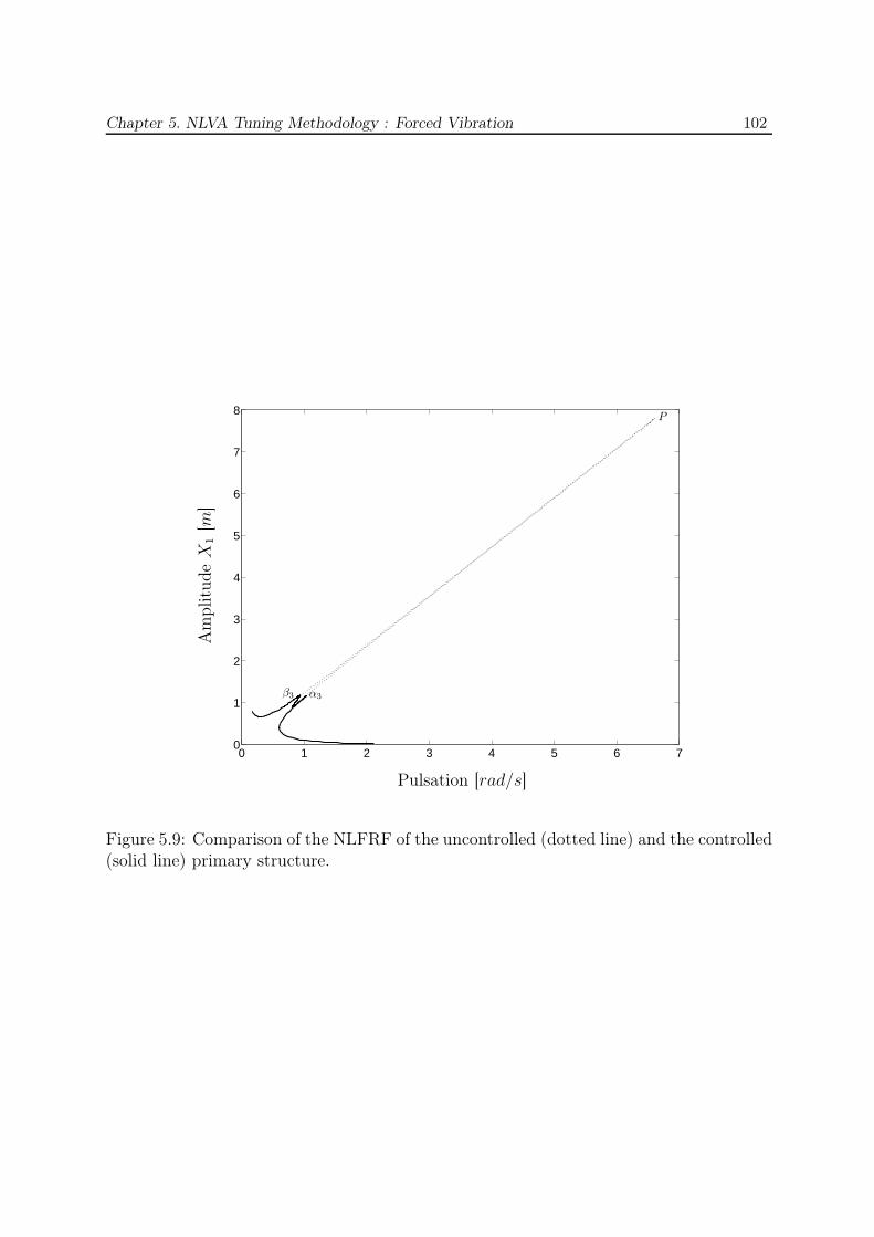
Chapter 5. NLVA Tuning Methodology : Forced Vibration 102
0 1 2 3 4 5 6 70
1
2
3
4
5
6
7
8
α3β3
P
Pulsation [rad/s]
Am
plitu
de
X1
[m]
Figure 5.9: Comparison of the NLFRF of the uncontrolled (dotted line) and the controlled(solid line) primary structure.
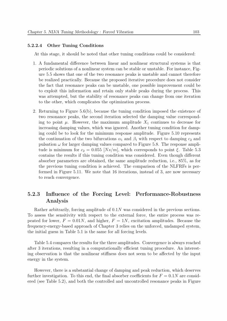
Chapter 5. NLVA Tuning Methodology : Forced Vibration 103
5.2.2.4 Other Tuning Conditions
At this stage, it should be noted that other tuning conditions could be considered:
1. A fundamental difference between linear and nonlinear structural systems is thatperiodic solutions of a nonlinear system can be stable or unstable. For instance, Fig-ure 5.5 shows that one of the two resonance peaks is unstable and cannot thereforebe realized practically. Because the proposed iterative procedure does not considerthe fact that resonance peaks can be unstable, one possible improvement could beto exploit this information and retain only stable peaks during the process. Thiswas attempted, but the stability of resonance peaks can change from one iterationto the other, which complicates the optimization process.
2. Returning to Figure 5.6(b), because the tuning condition imposed the existence oftwo resonance peaks, the second iteration selected the damping value correspond-ing to point µ. However, the maximum amplitude X1 continues to decrease forincreasing damping values, which was ignored. Another tuning condition for damp-ing could be to look for the minimum response amplitude. Figure 5.10 representsthe continuation of the two bifurcations α1 and β1 with respect to damping c2 andpulsation ω for larger damping values compared to Figure 5.8. The response ampli-tude is minimum for c2 = 0.055 [Ns/m], which corresponds to point ξ. Table 5.3contains the results if this tuning condition was considered. Even though differentabsorber parameters are obtained, the same amplitude reduction, i.e., 85%, as forthe previous tuning condition is achieved. The comparison of the NLFRFs is per-formed in Figure 5.11. We note that 16 iterations, instead of 3, are now necessaryto reach convergence.
5.2.3 Influence of the Forcing Level: Performance-Robustness
Analysis
Rather arbitrarily, forcing amplitude of 0.1N was considered in the previous sections.To assess the sensitivity with respect to the external force, the entire process was re-peated for lower, F = 0.01N , and higher, F = 1N , excitation amplitudes. Because thefrequency-energy-based approach of Chapter 3 relies on the unforced, undamped system,the initial guess in Table 5.1 is the same for all forcing levels.
Table 5.4 compares the results for the three amplitudes. Convergence is always reachedafter 3 iterations, resulting in a computationally efficient tuning procedure. An interest-ing observation is that the nonlinear stiffness does not seem to be affected by the inputenergy in the system.
However, there is a substantial change of damping and peak reduction, which deservesfurther investigation. To this end, the final absorber coefficients for F = 0.1N are consid-ered (see Table 5.2), and both the controlled and uncontrolled resonance peaks in Figure
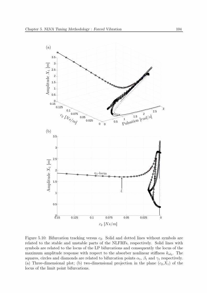
Chapter 5. NLVA Tuning Methodology : Forced Vibration 104
00.5
11.5
22.5
3
00.025
0.050.075
0.10.125
0.150
0.5
1
1.5
2
2.5
3
3.5
Pulsation [rad/
s]c2 [Ns/m]
Am
plitu
de
X1
[m]
(a)
00.0250.050.0750.10.1250.150
0.5
1
1.5
2
2.5
3
3.5
c2 [Ns/m]
Am
plitu
de
X1
[m]
ξ
(b)
α1-locus
Figure 5.10: Bifurcation tracking versus c2. Solid and dotted lines without symbols arerelated to the stable and unstable parts of the NLFRFs, respectively. Solid lines withsymbols are related to the locus of the LP bifurcations and consequently the locus of themaximum amplitude response with respect to the absorber nonlinear stiffness knl2 . Thesquares, circles and diamonds are related to bifurcation points α1, β1 and γ1 respectively.(a) Three-dimensional plot; (b) two-dimensional projection in the plane (c2,X1) of thelocus of the limit point bifurcations.

Chapter 5. NLVA Tuning Methodology : Forced Vibration 105
Iteration Variable knl2 c2 % of X1 reduction0 knl2 0.0076515 0.0020 651 c2 0.0076515 0.0550 772 knl2 0.0400 0.0550 81.53 c2 0.0400 0.0425 824 knl2 0.0280 0.0425 82.55 c2 0.0280 0.0355 836 knl2 0.0215 0.0355 83.38 c2 0.0215 0.0310 83.68 knl2 0.0174 0.0310 83.99 c2 0.0174 0.0275 84.110 knl2 0.0161 0.0275 84.311 c2 0.0161 0.0263 84.312 knl2 0.0135 0.0263 84.613 c2 0.0135 0.0238 84.814 knl2 0.0126 0.0238 84.915 c2 0.0126 0.0228 84.916 knl2 0.01222 0.0228 85
Table 5.3: Iterative procedure for knl2 and c2 optimization with minimal amplitude re-sponse as tuning condition for damping.
0 0.25 0.5 0.75 1 1.25 1.50
0.2
0.4
0.6
0.8
1
1.2
1.4
Pulsation [rad/s]
Am
plitu
de
X1
[m]
Figure 5.11: Comparison of the NLFRFs of the primary structure for two different tuningconditions applied to the damping (solid line and dotted line refers to Tables 5.3 and 5.2,respectively).
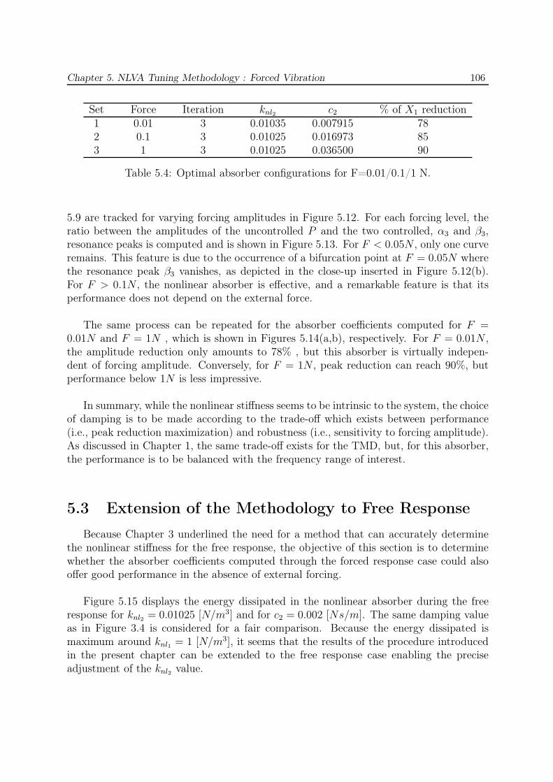
Chapter 5. NLVA Tuning Methodology : Forced Vibration 106
Set Force Iteration knl2 c2 % of X1 reduction1 0.01 3 0.01035 0.007915 782 0.1 3 0.01025 0.016973 853 1 3 0.01025 0.036500 90
Table 5.4: Optimal absorber configurations for F=0.01/0.1/1 N.
5.9 are tracked for varying forcing amplitudes in Figure 5.12. For each forcing level, theratio between the amplitudes of the uncontrolled P and the two controlled, α3 and β3,resonance peaks is computed and is shown in Figure 5.13. For F < 0.05N , only one curveremains. This feature is due to the occurrence of a bifurcation point at F = 0.05N wherethe resonance peak β3 vanishes, as depicted in the close-up inserted in Figure 5.12(b).For F > 0.1N , the nonlinear absorber is effective, and a remarkable feature is that itsperformance does not depend on the external force.
The same process can be repeated for the absorber coefficients computed for F =0.01N and F = 1N , which is shown in Figures 5.14(a,b), respectively. For F = 0.01N ,the amplitude reduction only amounts to 78% , but this absorber is virtually indepen-dent of forcing amplitude. Conversely, for F = 1N , peak reduction can reach 90%, butperformance below 1N is less impressive.
In summary, while the nonlinear stiffness seems to be intrinsic to the system, the choiceof damping is to be made according to the trade-off which exists between performance(i.e., peak reduction maximization) and robustness (i.e., sensitivity to forcing amplitude).As discussed in Chapter 1, the same trade-off exists for the TMD, but, for this absorber,the performance is to be balanced with the frequency range of interest.
5.3 Extension of the Methodology to Free Response
Because Chapter 3 underlined the need for a method that can accurately determinethe nonlinear stiffness for the free response, the objective of this section is to determinewhether the absorber coefficients computed through the forced response case could alsooffer good performance in the absence of external forcing.
Figure 5.15 displays the energy dissipated in the nonlinear absorber during the freeresponse for knl2 = 0.01025 [N/m3] and for c2 = 0.002 [Ns/m]. The same damping valueas in Figure 3.4 is considered for a fair comparison. Because the energy dissipated ismaximum around knl1 = 1 [N/m3], it seems that the results of the procedure introducedin the present chapter can be extended to the free response case enabling the preciseadjustment of the knl2 value.
Chapter 5. NLVA Tuning Methodology : Forced Vibration 107
05
1015
2025
00.2
0.40.6
0.810
5
10
15
20
25
Pulsation [rad/
s]Force [N ]
Am
plitu
de
X1
[m]
(a)
00.10.20.30.40.50.60.70.80.910
5
10
15
20
25
Force [n]
Am
plitu
de
X1
[m]
(b)
00.020.040.060.080.10.120.140.160.180.20
1
2
3
4
5
6
7
8
9
α3-locus
β3-locus
P -locus
α3-locus
β3-locus
P-locus
Figure 5.12: Locus of the primary structure maximum response amplitude (P ,α3,β3). Theline with circles stands for the locus of maxima in the uncontrolled configuration whereasthe lines with squares correspond to the locus of maxima in the controlled configuration(a) Three-dimensional graph; (b) 2D projection in the plane (X1,F ).

Chapter 5. NLVA Tuning Methodology : Forced Vibration 108
0 0.1 0.2 0.3 0.4 0.5 0.6 0.7 0.8 0.9 10
10
20
30
40
50
60
70
80
90
100
Force [N ]
Per
centa
geof
amplitu
de
X1
reduct
ion
[%]
Figure 5.13: Percentage of maximal amplitude reduction with respect to the excitationlevel F. Dotted and solid lines refer to peaks α3 and β3 of Figure 5.9, respectively.
0 1 2 3 4 5 6 7 8 9 100
10
20
30
40
50
60
70
80
90
100
Force [N ]
%ofX
1re
duct
ion
(a)
0 0.1 0.2 0.3 0.4 0.5 0.6 0.7 0.8 0.9 10
10
20
30
40
50
60
70
80
90
100
Force [N ]
%ofX
1re
duct
ion
(b)
Figure 5.14: (a) Performance - robustness curves of the nonlinear absorber with the solid,dashed and dotted lines corresponding to the set of absorber parameter 1, 2 and 3 (Table5.4), respectively. (b) Close-up for low energy levels.
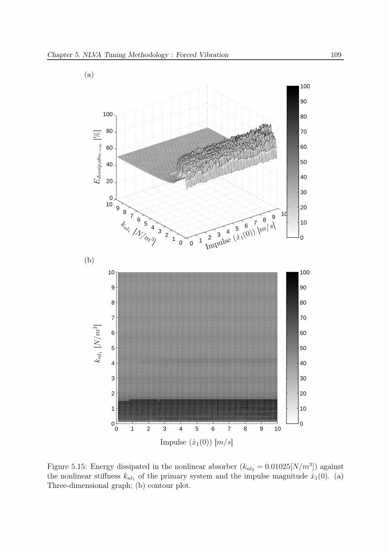
Chapter 5. NLVA Tuning Methodology : Forced Vibration 109
0 1 2 3 4 5 6 7 8 9 10
01
23
45
67
89
100
20
40
60
80
100
0
10
20
30
40
50
60
70
80
90
100
Impulse (x1(0)) [m/s]
knl1 [N/m 3
]
Edis
sip,a
bst→
∞[%
]
(a)
0 1 2 3 4 5 6 7 8 9 100
1
2
3
4
5
6
7
8
9
10
0
10
20
30
40
50
60
70
80
90
100
Impulse (x1(0)) [m/s]
knl 1
[N/m
3]
(b)
Figure 5.15: Energy dissipated in the nonlinear absorber (knl2 = 0.01025[N/m3]) againstthe nonlinear stiffness knl1 of the primary system and the impulse magnitude x1(0). (a)Three-dimensional graph; (b) contour plot.
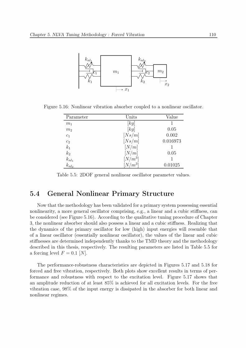
Chapter 5. NLVA Tuning Methodology : Forced Vibration 110
knl1 knl2
c1 c2
k1 k2
m1 m2
x1
x2
Figure 5.16: Nonlinear vibration absorber coupled to a nonlinear oscillator.
Parameter Units Valuem1 [kg] 1m2 [kg] 0.05c1 [Ns/m] 0.002c2 [Ns/m] 0.016973k1 [N/m] 1k2 [N/m] 0.05knl1 [N/m3] 1knl2 [N/m3] 0.01025
Table 5.5: 2DOF general nonlinear oscillator parameter values.
5.4 General Nonlinear Primary Structure
Now that the methodology has been validated for a primary system possessing essentialnonlinearity, a more general oscillator comprising, e.g., a linear and a cubic stiffness, canbe considered (see Figure 5.16). According to the qualitative tuning procedure of Chapter3, the nonlinear absorber should also possess a linear and a cubic stiffness. Realizing thatthe dynamics of the primary oscillator for low (high) input energies will resemble thatof a linear oscillator (essentially nonlinear oscillator), the values of the linear and cubicstiffnesses are determined independently thanks to the TMD theory and the methodologydescribed in this thesis, respectively. The resulting parameters are listed in Table 5.5 fora forcing level F = 0.1 [N ].
The performance-robustness characteristics are depicted in Figures 5.17 and 5.18 forforced and free vibration, respectively. Both plots show excellent results in terms of per-formance and robustness with respect to the excitation level. Figure 5.17 shows thatan amplitude reduction of at least 85% is achieved for all excitation levels. For the freevibration case, 98% of the input energy is dissipated in the absorber for both linear andnonlinear regimes.
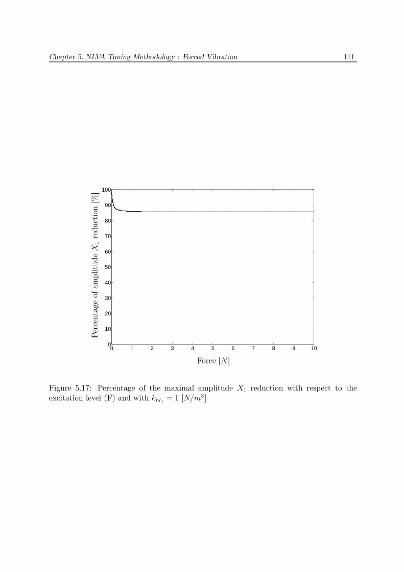
Chapter 5. NLVA Tuning Methodology : Forced Vibration 111
0 1 2 3 4 5 6 7 8 9 100
10
20
30
40
50
60
70
80
90
100
Force [N ]
Per
centa
geof
amplitu
de
X1
reduct
ion
[%]
Figure 5.17: Percentage of the maximal amplitude X1 reduction with respect to theexcitation level (F) and with knl1 = 1 [N/m3]
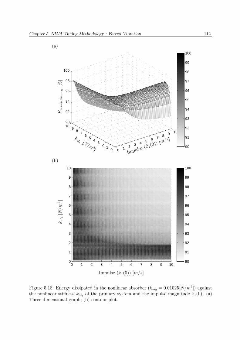
Chapter 5. NLVA Tuning Methodology : Forced Vibration 112
0 1 2 3 4 5 6 7 8 9 10
01
23
45
67
89
1090
92
94
96
98
100
90
91
92
93
94
95
96
97
98
99
100
Impulse (x1(0)) [m/s]
knl1 [N/m 3
]
Edis
sip,a
bst→
∞[%
]
(a)
0 1 2 3 4 5 6 7 8 9 100
1
2
3
4
5
6
7
8
9
10
90
91
92
93
94
95
96
97
98
99
100
Impulse (x1(0)) [m/s]
knl 1
[N/m
3]
(b)
Figure 5.18: Energy dissipated in the nonlinear absorber (knl2 = 0.01025[N/m3]) againstthe nonlinear stiffness knl1 of the primary system and the impulse magnitude x1(0). (a)Three-dimensional graph; (b) contour plot.
Chapter 5. NLVA Tuning Methodology : Forced Vibration 113
5.5 Concluding Remarks
This chapter proposed an integrated methodology for tuning NLVAs possessing lin-ear and nonlinear stiffnesses. The key feature of this methodology is that both free andforced vibrations of a nonlinear primary system can be mitigated in a wide range of inputenergies.
As illustrated in Figure 5.19, the first step of the procedure consists in identifying theparameters of the primary structure, i.e., m1 and c1 together with the functional form ofthe nonlinear stiffness. If the primary system possesses a linear stiffness k1, the tuning ofa TMD on the underlying linear primary system is carried out, which determines the ab-sorber linear stiffness k2opt and damping c2optl
. The absorber mass m2 is chosen accordingto practical constraints, e.g., it can be set to 5% of the total system mass.
The procedure continues by considering the undamped, unforced dynamics of the un-derlying nonlinear system, as reported in Chapter 3. An appropriate functional form forthe absorber nonlinearity is selected by matching the backbone of the absorber FEP withthat (the mode of interest) of a SDOF (MDOF) primary system. Through this backbonematch, an initial guess for the absorber nonlinear stiffness knl2 is also calculated. Theabsorber damping c2nl
is chosen to be equal to the damping of the primary structure c1.
To refine the values of the absorber nonlinear stiffness and damping, the forced re-sponse is considered, as proposed in the present chapter. The forcing amplitude is selectedby keeping in mind that the absorber will be robust for larger forcing amplitudes. A NL-FRF is computed, and its bifurcation points are localized. The optimization of the non-linear stiffness knl2 is performed through bifurcation tracking by reducing the amplitudeX1 of the primary system while ensuring two resonance peaks with the same amplitude.Damping optimization is also achieved through bifurcation tracking by reducing the am-plitude X1 until a single resonance peak remains. The sequential optimization of knl2 andc2nl
is continued until one tuning condition can no longer be satisfied, which leads to theset of parameters (knl2opt
,c2optnl).
At this stage, two different absorber damping values c2optland c2optnl
are computed;damping selection results from a tradeoff. Choosing the absorber damping to be c2optl
gives more importance to the dynamics at low-energy level and ensures that the per-formance will be insensitive to TMD mistuning. Conversely, by choosing the absorberdamping to be c2optnl
, the performance for higher energies will be more robust againstvariation of input energy. Eventually, an adequate set of absorber parameters is obtained,namely k2opt, knl2opt
and c2opt .

Chapter 5. NLVA Tuning Methodology : Forced Vibration 114
Primary
system identification
Stiffness functional form,
m1,c1
L = 0NO Presence
ofLinearity ?
YESL = 1
NLVA tuning for the under-
lying nonlinear primary system
TMD tuning for the under-
lying linear primary system
Optimal stiffness k2
k2m2
=k1m1
, or
cf Tables A.1 and A.3
Optimal damping c2l
cf Tables A.1 and A.3
Optimal
tuning of the TMD
k2opt, c2optl
Fundamental dynamics
characterization
Frequency-energy plot
computation
Initial guess
absorber parameters
knl2through FEP Matching
c2nl= c1
Choice of the
Excitation Level F
Robustness for
forcing amplitudes > F
Bifurcation points
localization
NLFRF computation
with related bifurcation points
Bifurcations tracking
knl2optimization
X1 reduction and 2 resonance
peaks at same amplitude
Bifurcations tracking
c2nloptimization
X1 reduction and
existence of 2 resonance peaksYES
YES
NO
NO
Optimal
tuning of the NLVA
knl2opt, c2optnl
Damping selection
If L=0 If L=1
c2opt
=c2optnl
c2opt
=[c2optl
,c2optnl]
Optimal
tuning of the absorber
k2opt, knl2opt
,
c2opt
Free
Vib
ratio
n
Frequency-Energy
Procedure
Forced
Vib
ratio
n
Bifurcatio
nA
naly
sis
Figure 5.19: Flowchart of the NLVA integrated tuning procedure.
Chapter 6
Tuning of a Nonlinear Vibration
Absorber to Suppress Limit Cycle
Oscillations
Abstract
This chapter proposes to suppress limit cycle oscillations, which are a persis-tent problem in engineering applications, using a nonlinear vibration absorber.Specifically, the stabilization of torsional vibrations of a drill-string system isaddressed. A nonlinear vibration absorber with cubic stiffness is first consid-ered, and bifurcation analysis is exploited for computing adequate absorber pa-rameters. The determination of an appropriate functional form for the absorberbased on the tuning procedure of the previous chapters is briefly discussed.
115
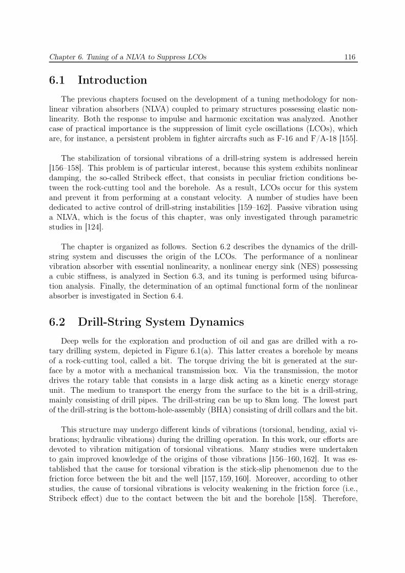
Chapter 6. Tuning of a NLVA to Suppress LCOs 116
6.1 Introduction
The previous chapters focused on the development of a tuning methodology for non-linear vibration absorbers (NLVA) coupled to primary structures possessing elastic non-linearity. Both the response to impulse and harmonic excitation was analyzed. Anothercase of practical importance is the suppression of limit cycle oscillations (LCOs), whichare, for instance, a persistent problem in fighter aircrafts such as F-16 and F/A-18 [155].
The stabilization of torsional vibrations of a drill-string system is addressed herein[156–158]. This problem is of particular interest, because this system exhibits nonlineardamping, the so-called Stribeck effect, that consists in peculiar friction conditions be-tween the rock-cutting tool and the borehole. As a result, LCOs occur for this systemand prevent it from performing at a constant velocity. A number of studies have beendedicated to active control of drill-string instabilities [159–162]. Passive vibration usinga NLVA, which is the focus of this chapter, was only investigated through parametricstudies in [124].
The chapter is organized as follows. Section 6.2 describes the dynamics of the drill-string system and discusses the origin of the LCOs. The performance of a nonlinearvibration absorber with essential nonlinearity, a nonlinear energy sink (NES) possessinga cubic stiffness, is analyzed in Section 6.3, and its tuning is performed using bifurca-tion analysis. Finally, the determination of an optimal functional form of the nonlinearabsorber is investigated in Section 6.4.
6.2 Drill-String System Dynamics
Deep wells for the exploration and production of oil and gas are drilled with a ro-tary drilling system, depicted in Figure 6.1(a). This latter creates a borehole by meansof a rock-cutting tool, called a bit. The torque driving the bit is generated at the sur-face by a motor with a mechanical transmission box. Via the transmission, the motordrives the rotary table that consists in a large disk acting as a kinetic energy storageunit. The medium to transport the energy from the surface to the bit is a drill-string,mainly consisting of drill pipes. The drill-string can be up to 8km long. The lowest partof the drill-string is the bottom-hole-assembly (BHA) consisting of drill collars and the bit.
This structure may undergo different kinds of vibrations (torsional, bending, axial vi-brations; hydraulic vibrations) during the drilling operation. In this work, our efforts aredevoted to vibration mitigation of torsional vibrations. Many studies were undertakento gain improved knowledge of the origins of those vibrations [156–160, 162]. It was es-tablished that the cause for torsional vibration is the stick-slip phenomenon due to thefriction force between the bit and the well [157, 159, 160]. Moreover, according to otherstudies, the cause of torsional vibrations is velocity weakening in the friction force (i.e.,Stribeck effect) due to the contact between the bit and the borehole [158]. Therefore,
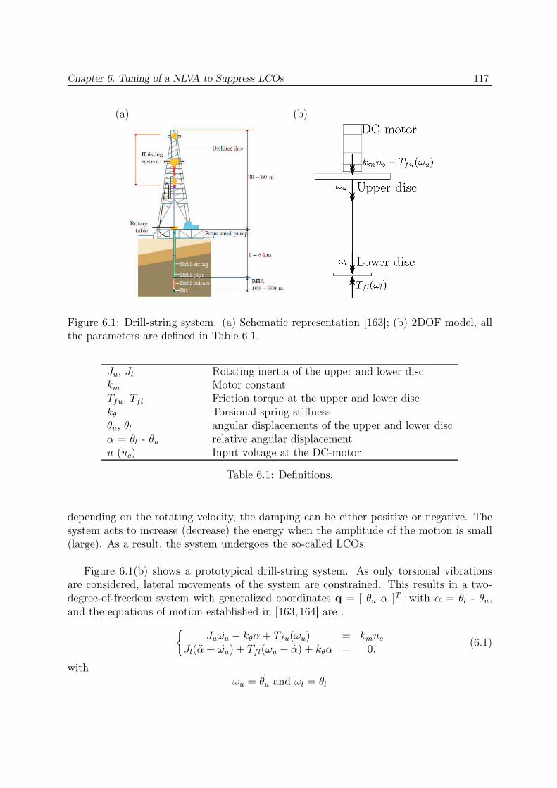
Chapter 6. Tuning of a NLVA to Suppress LCOs 117
(a) (b)
Figure 6.1: Drill-string system. (a) Schematic representation [163]; (b) 2DOF model, allthe parameters are defined in Table 6.1.
Ju, Jl Rotating inertia of the upper and lower disckm Motor constantTfu, Tfl Friction torque at the upper and lower disckθ Torsional spring stiffnessθu, θl angular displacements of the upper and lower discα = θl - θu relative angular displacementu (uc) Input voltage at the DC-motor
Table 6.1: Definitions.
depending on the rotating velocity, the damping can be either positive or negative. Thesystem acts to increase (decrease) the energy when the amplitude of the motion is small(large). As a result, the system undergoes the so-called LCOs.
Figure 6.1(b) shows a prototypical drill-string system. As only torsional vibrationsare considered, lateral movements of the system are constrained. This results in a two-degree-of-freedom system with generalized coordinates q = [ θu α ]T , with α = θl - θu,and the equations of motion established in [163, 164] are :
{
Juωu − kθα + Tfu(ωu) = kmuc
Jl(α + ωu) + Tfl(ωu + α) + kθα = 0.(6.1)
withωu = θu and ωl = θl
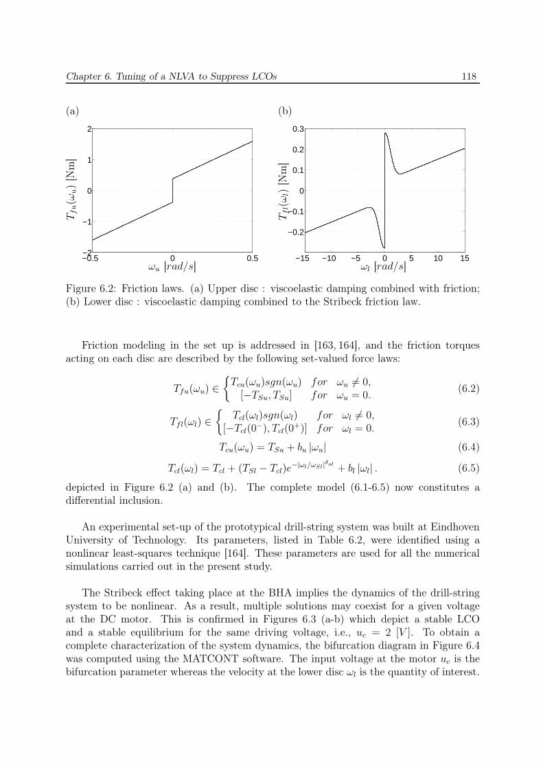
Chapter 6. Tuning of a NLVA to Suppress LCOs 118
−0.5 0 0.5−2
−1
0
1
2
−15 −10 −5 0 5 10 15
−0.2
−0.1
0
0.1
0.2
0.3
(a) (b)
ωu [rad/s]
Tfu(ω
u)
[Nm
]
ωl [rad/s]
Tfl(ω
l)[N
m]
Figure 6.2: Friction laws. (a) Upper disc : viscoelastic damping combined with friction;(b) Lower disc : viscoelastic damping combined to the Stribeck friction law.
Friction modeling in the set up is addressed in [163, 164], and the friction torquesacting on each disc are described by the following set-valued force laws:
Tfu(ωu) ∈{
Tcu(ωu)sgn(ωu) for ωu 6= 0,[−TSu, TSu] for ωu = 0.
(6.2)
Tfl(ωl) ∈{
Tcl(ωl)sgn(ωl) for ωl 6= 0,[−Tcl(0
−), Tcl(0+)] for ωl = 0.
(6.3)
Tcu(ωu) = TSu + bu |ωu| (6.4)
Tcl(ωl) = Tcl + (TSl − Tcl)e−|ωl/ωSl|δsl
+ bl |ωl| . (6.5)
depicted in Figure 6.2 (a) and (b). The complete model (6.1-6.5) now constitutes adifferential inclusion.
An experimental set-up of the prototypical drill-string system was built at EindhovenUniversity of Technology. Its parameters, listed in Table 6.2, were identified using anonlinear least-squares technique [164]. These parameters are used for all the numericalsimulations carried out in the present study.
The Stribeck effect taking place at the BHA implies the dynamics of the drill-stringsystem to be nonlinear. As a result, multiple solutions may coexist for a given voltageat the DC motor. This is confirmed in Figures 6.3 (a-b) which depict a stable LCOand a stable equilibrium for the same driving voltage, i.e., uc = 2 [V ]. To obtain acomplete characterization of the system dynamics, the bifurcation diagram in Figure 6.4was computed using the MATCONT software. The input voltage at the motor uc is thebifurcation parameter whereas the velocity at the lower disc ωl is the quantity of interest.
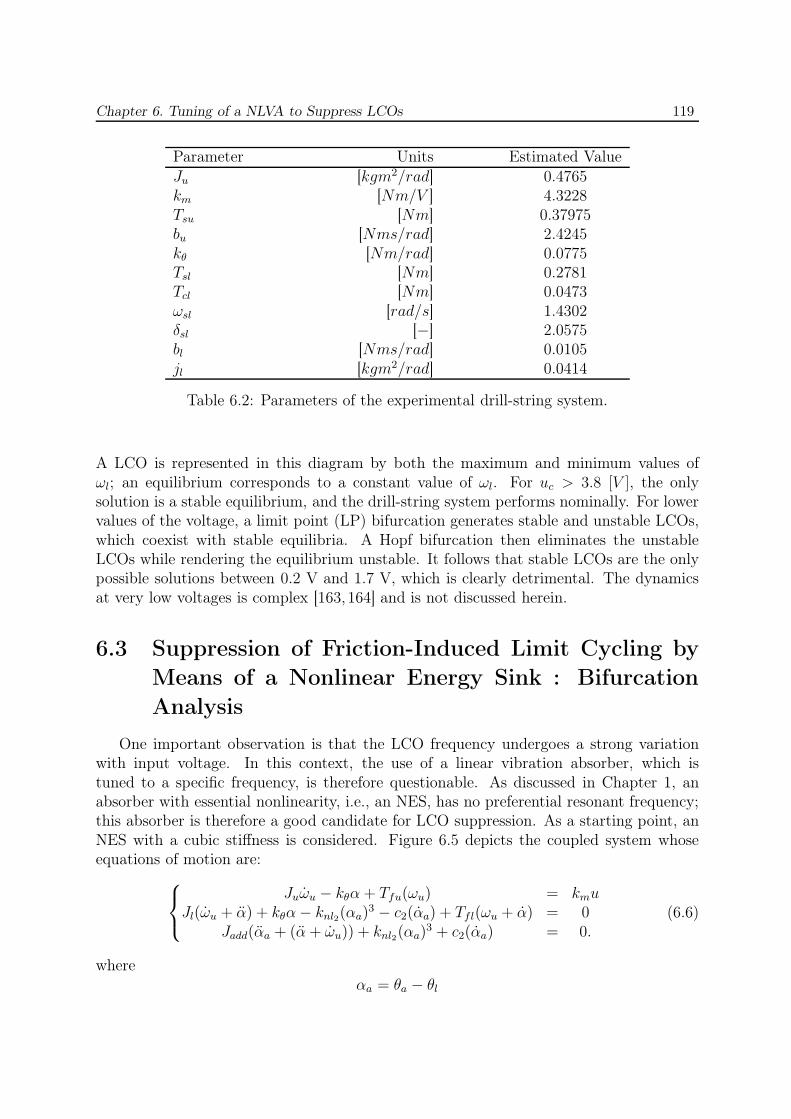
Chapter 6. Tuning of a NLVA to Suppress LCOs 119
Parameter Units Estimated ValueJu [kgm2/rad] 0.4765km [Nm/V ] 4.3228Tsu [Nm] 0.37975bu [Nms/rad] 2.4245kθ [Nm/rad] 0.0775Tsl [Nm] 0.2781Tcl [Nm] 0.0473ωsl [rad/s] 1.4302δsl [−] 2.0575bl [Nms/rad] 0.0105jl [kgm2/rad] 0.0414
Table 6.2: Parameters of the experimental drill-string system.
A LCO is represented in this diagram by both the maximum and minimum values ofωl; an equilibrium corresponds to a constant value of ωl. For uc > 3.8 [V ], the onlysolution is a stable equilibrium, and the drill-string system performs nominally. For lowervalues of the voltage, a limit point (LP) bifurcation generates stable and unstable LCOs,which coexist with stable equilibria. A Hopf bifurcation then eliminates the unstableLCOs while rendering the equilibrium unstable. It follows that stable LCOs are the onlypossible solutions between 0.2 V and 1.7 V, which is clearly detrimental. The dynamicsat very low voltages is complex [163, 164] and is not discussed herein.
6.3 Suppression of Friction-Induced Limit Cycling by
Means of a Nonlinear Energy Sink : Bifurcation
Analysis
One important observation is that the LCO frequency undergoes a strong variationwith input voltage. In this context, the use of a linear vibration absorber, which istuned to a specific frequency, is therefore questionable. As discussed in Chapter 1, anabsorber with essential nonlinearity, i.e., an NES, has no preferential resonant frequency;this absorber is therefore a good candidate for LCO suppression. As a starting point, anNES with a cubic stiffness is considered. Figure 6.5 depicts the coupled system whoseequations of motion are:
Juωu − kθα + Tfu(ωu) = kmuJl(ωu + α) + kθα − knl2(αa)
3 − c2(αa) + Tfl(ωu + α) = 0Jadd(αa + (α + ωu)) + knl2(αa)
3 + c2(αa) = 0.(6.6)
whereαa = θa − θl
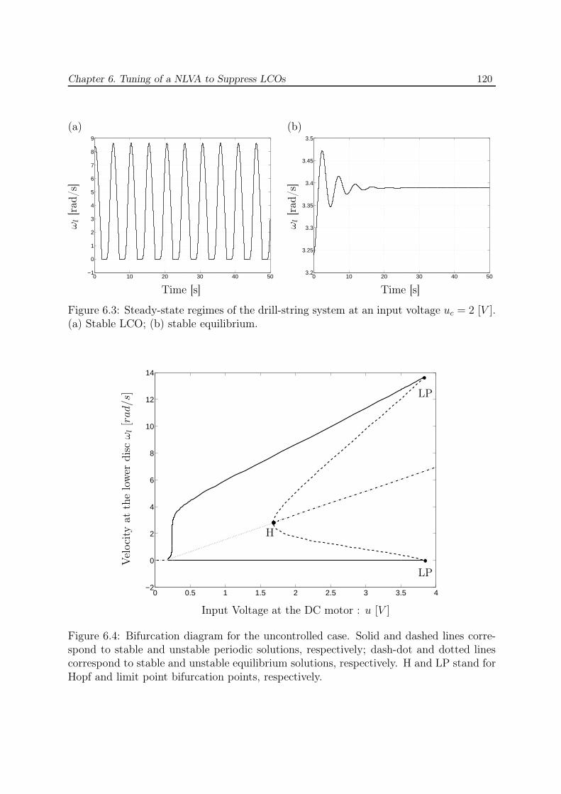
Chapter 6. Tuning of a NLVA to Suppress LCOs 120
0 10 20 30 40 50−1
0
1
2
3
4
5
6
7
8
9
0 10 20 30 40 503.2
3.25
3.3
3.35
3.4
3.45
3.5
(a) (b)
Time [s]
ωl[r
ad/s
]
Time [s]ω
l[r
ad/s
]
Figure 6.3: Steady-state regimes of the drill-string system at an input voltage uc = 2 [V ].(a) Stable LCO; (b) stable equilibrium.
0 0.5 1 1.5 2 2.5 3 3.5 4−2
0
2
4
6
8
10
12
14
Input Voltage at the DC motor : u [V ]
Vel
oci
tyat
the
low
erdis
cω
l[r
ad/s
]
LP
LP
H
Figure 6.4: Bifurcation diagram for the uncontrolled case. Solid and dashed lines corre-spond to stable and unstable periodic solutions, respectively; dash-dot and dotted linescorrespond to stable and unstable equilibrium solutions, respectively. H and LP stand forHopf and limit point bifurcation points, respectively.
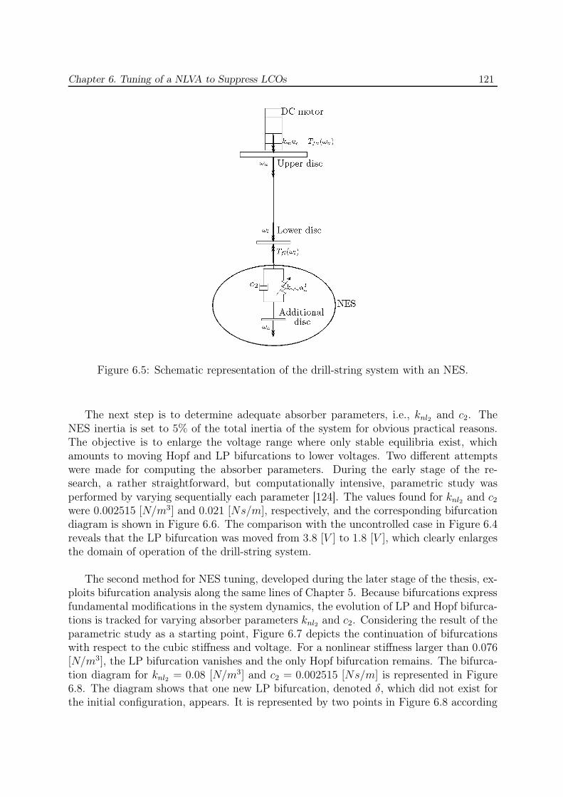
Chapter 6. Tuning of a NLVA to Suppress LCOs 121
Figure 6.5: Schematic representation of the drill-string system with an NES.
The next step is to determine adequate absorber parameters, i.e., knl2 and c2. TheNES inertia is set to 5% of the total inertia of the system for obvious practical reasons.The objective is to enlarge the voltage range where only stable equilibria exist, whichamounts to moving Hopf and LP bifurcations to lower voltages. Two different attemptswere made for computing the absorber parameters. During the early stage of the re-search, a rather straightforward, but computationally intensive, parametric study wasperformed by varying sequentially each parameter [124]. The values found for knl2 and c2
were 0.002515 [N/m3] and 0.021 [Ns/m], respectively, and the corresponding bifurcationdiagram is shown in Figure 6.6. The comparison with the uncontrolled case in Figure 6.4reveals that the LP bifurcation was moved from 3.8 [V ] to 1.8 [V ], which clearly enlargesthe domain of operation of the drill-string system.
The second method for NES tuning, developed during the later stage of the thesis, ex-ploits bifurcation analysis along the same lines of Chapter 5. Because bifurcations expressfundamental modifications in the system dynamics, the evolution of LP and Hopf bifurca-tions is tracked for varying absorber parameters knl2 and c2. Considering the result of theparametric study as a starting point, Figure 6.7 depicts the continuation of bifurcationswith respect to the cubic stiffness and voltage. For a nonlinear stiffness larger than 0.076[N/m3], the LP bifurcation vanishes and the only Hopf bifurcation remains. The bifurca-tion diagram for knl2 = 0.08 [N/m3] and c2 = 0.002515 [Ns/m] is represented in Figure6.8. The diagram shows that one new LP bifurcation, denoted δ, which did not exist forthe initial configuration, appears. It is represented by two points in Figure 6.8 according
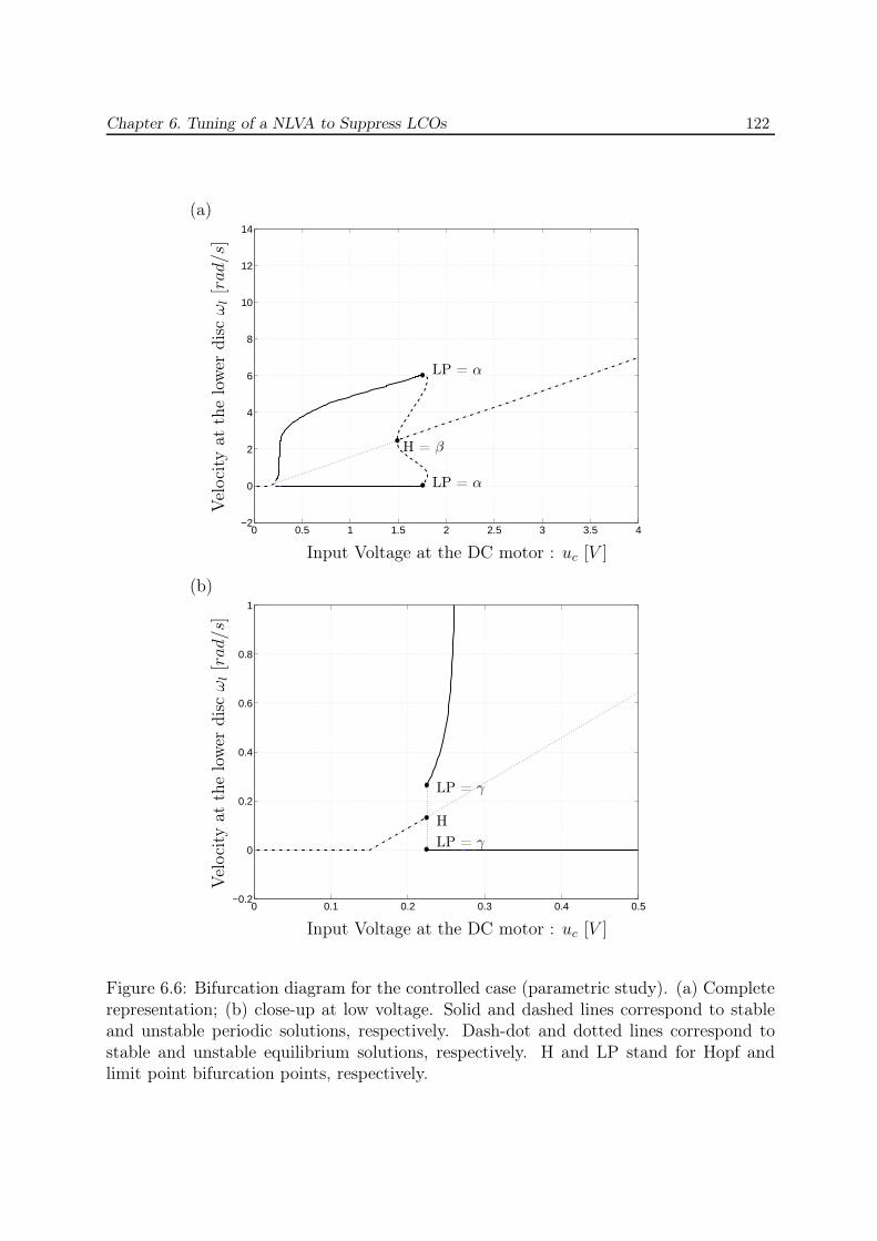
Chapter 6. Tuning of a NLVA to Suppress LCOs 122
0 0.5 1 1.5 2 2.5 3 3.5 4−2
0
2
4
6
8
10
12
14
0 0.1 0.2 0.3 0.4 0.5−0.2
0
0.2
0.4
0.6
0.8
1
Input Voltage at the DC motor : uc [V ]
Vel
oci
tyat
the
low
erdis
cω
l[r
ad/s
](a)
Input Voltage at the DC motor : uc [V ]
Vel
oci
tyat
the
low
erdis
cω
l[r
ad/s
]
(b)
LP = α
LP = α
H = β
LP = γ
LP = γ
H
Figure 6.6: Bifurcation diagram for the controlled case (parametric study). (a) Completerepresentation; (b) close-up at low voltage. Solid and dashed lines correspond to stableand unstable periodic solutions, respectively. Dash-dot and dotted lines correspond tostable and unstable equilibrium solutions, respectively. H and LP stand for Hopf andlimit point bifurcation points, respectively.
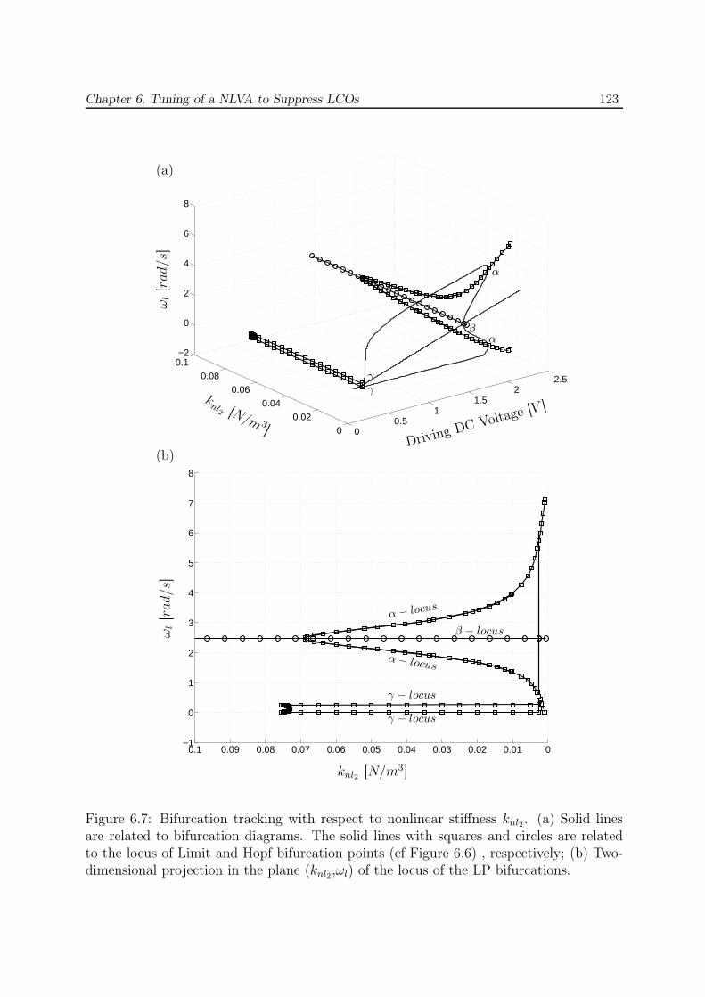
Chapter 6. Tuning of a NLVA to Suppress LCOs 123
00.5
11.5
22.5
00.02
0.040.06
0.080.1−2
0
2
4
6
8
Driving DC Voltage [V ]
knl2 [N/m 3
]
ωl[r
ad/s
](a)
00.010.020.030.040.050.060.070.080.090.1−1
0
1
2
3
4
5
6
7
8
knl2 [N/m3]
ωl[r
ad/s
]
(b)
α
αβ
γγ
α − locus
α − locus
β − locus
γ − locus
γ − locus
Figure 6.7: Bifurcation tracking with respect to nonlinear stiffness knl2. (a) Solid linesare related to bifurcation diagrams. The solid lines with squares and circles are relatedto the locus of Limit and Hopf bifurcation points (cf Figure 6.6) , respectively; (b) Two-dimensional projection in the plane (knl2,ωl) of the locus of the LP bifurcations.

Chapter 6. Tuning of a NLVA to Suppress LCOs 124
0 0.5 1 1.5 2 2.5 3 3.5−2
0
2
4
6
8
10
12
Input Voltage at the DC motor : u [V ]
Vel
oci
tyat
the
low
erdis
cω
l[r
ad/s
]
δ=LP
δ=LP
Figure 6.8: Bifurcation diagram for the controlled case (first iteration of bifurcation track-ing, knl2 = 0.0035 [N/m3], c2 = 0.021 [Ns/m]).
the chosen convention (i.e., a LCO is drawn at both the maximum and minimum valuesof ωl). This highlights the importance of computing the bifurcation diagram after eachiteration so as not to miss any dynamics. We also note that a similar observation wasmade in Section 5.2.2.2. This new LP bifurcation should therefore be tracked back inparameter space, which is carried out in Figure 6.9. The close-up in Figure 6.9(b) illus-trates that the new bifurcation is generated from knl2 = 0.00351 [N/m3]. Summarizing,if knl2 = 0.0035 [N/m3], the new LP bifurcation does not yet exist, but the original LPbifurcation is associated with a lower voltage (1.75 [V ] instead of 1.8 [V ]), which resultsin an (admittedly small) improvement.
Now that the first iteration is finalized, subsequent iterations can be performed byvarying damping and cubic stiffness sequentially. The results are displayed in Table 6.3and in Figure 6.10. A comparison between the bifurcation diagrams of the uncontrolled,controlled (parametric study and bifurcation analysis) is plotted in Figure 6.11. It pointsout that (i) the NES can substantially enlarge the domain of operation of the drill-string system; (ii) the amplitudes of the remaining LCOs are smaller than those of theuncontrolled case, and (iii) bifurcation analysis leads to better results than the parametricstudy with much less computational burden.
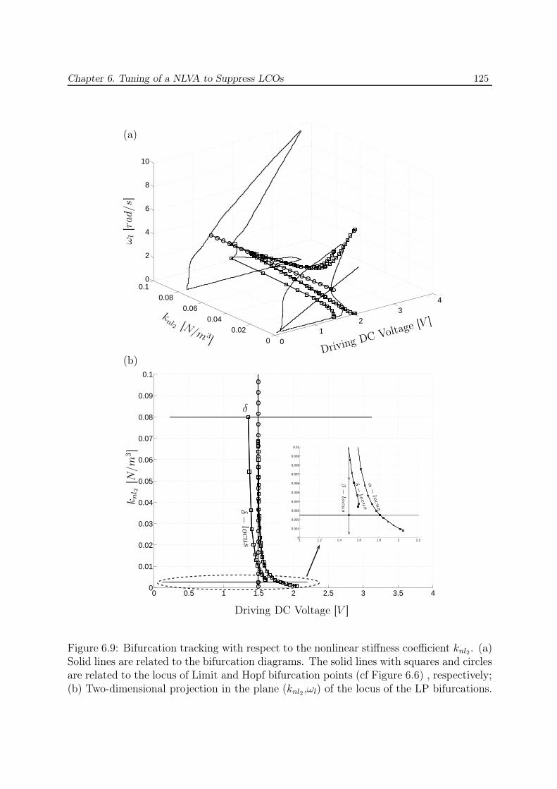
Chapter 6. Tuning of a NLVA to Suppress LCOs 125
01
23
4
00.02
0.040.06
0.080.1
0
2
4
6
8
10
Driving DC Voltage [V ]
knl2 [N/m 3
]
ωl[r
ad/s
](a)
0 0.5 1 1.5 2 2.5 3 3.5 40
0.01
0.02
0.03
0.04
0.05
0.06
0.07
0.08
0.09
0.1
Driving DC Voltage [V ]
knl 2
[N/m
3]
(b)
1 1.2 1.4 1.6 1.8 2 2.20
0.001
0.002
0.003
0.004
0.005
0.006
0.007
0.008
0.009
0.01
δ
δ −locu
s
α−
locu
s
δ−
locu
s
β−
locu
s
Figure 6.9: Bifurcation tracking with respect to the nonlinear stiffness coefficient knl2. (a)Solid lines are related to the bifurcation diagrams. The solid lines with squares and circlesare related to the locus of Limit and Hopf bifurcation points (cf Figure 6.6) , respectively;(b) Two-dimensional projection in the plane (knl2 ,ωl) of the locus of the LP bifurcations.
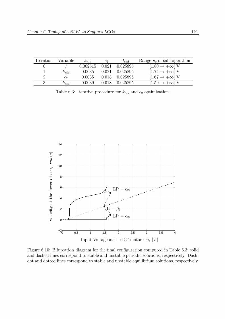
Chapter 6. Tuning of a NLVA to Suppress LCOs 126
Iteration Variable knl2 c2 Jadd Range uc of safe operation0 / 0.002515 0.021 0.025895 [1.80 → +∞[ V1 knl2 0.0035 0.021 0.025895 [1.74 → +∞[ V2 c2 0.0035 0.018 0.025895 [1.67 → +∞[ V3 knl2 0.0039 0.018 0.025895 [1.59 → +∞[ V
Table 6.3: Iterative procedure for knl2 and c2 optimization.
0 0.5 1 1.5 2 2.5 3 3.5 4−2
0
2
4
6
8
10
12
14
Input Voltage at the DC motor : uc [V ]
Vel
oci
tyat
the
low
erdis
cω
l[r
ad/s
]
LP = α3
LP = α3
H = β3
Figure 6.10: Bifurcation diagram for the final configuration computed in Table 6.3; solidand dashed lines correspond to stable and unstable periodic solutions, respectively. Dash-dot and dotted lines correspond to stable and unstable equilibrium solutions, respectively.
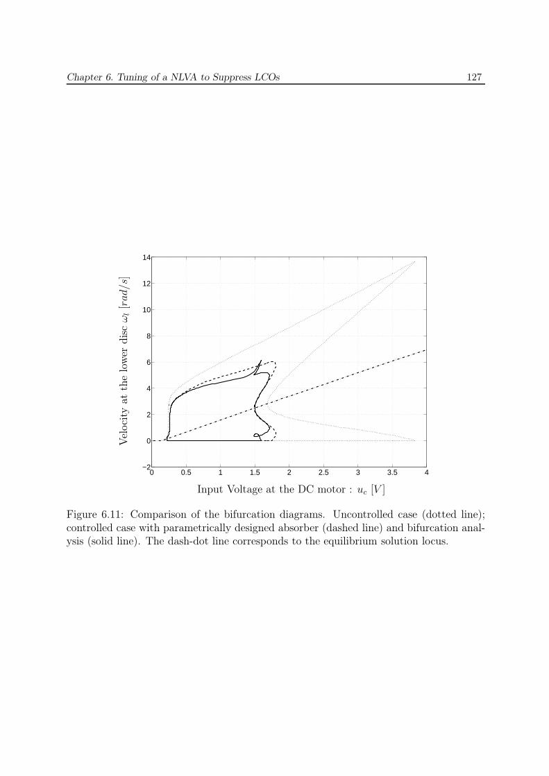
Chapter 6. Tuning of a NLVA to Suppress LCOs 127
0 0.5 1 1.5 2 2.5 3 3.5 4−2
0
2
4
6
8
10
12
14
Input Voltage at the DC motor : uc [V ]
Vel
oci
tyat
the
low
erdis
cω
l[r
ad/s
]
Figure 6.11: Comparison of the bifurcation diagrams. Uncontrolled case (dotted line);controlled case with parametrically designed absorber (dashed line) and bifurcation anal-ysis (solid line). The dash-dot line corresponds to the equilibrium solution locus.
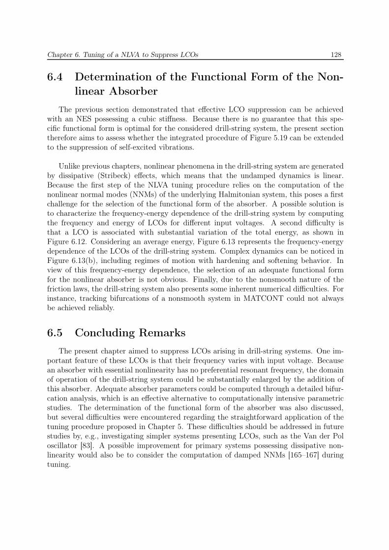
Chapter 6. Tuning of a NLVA to Suppress LCOs 128
6.4 Determination of the Functional Form of the Non-
linear Absorber
The previous section demonstrated that effective LCO suppression can be achievedwith an NES possessing a cubic stiffness. Because there is no guarantee that this spe-cific functional form is optimal for the considered drill-string system, the present sectiontherefore aims to assess whether the integrated procedure of Figure 5.19 can be extendedto the suppression of self-excited vibrations.
Unlike previous chapters, nonlinear phenomena in the drill-string system are generatedby dissipative (Stribeck) effects, which means that the undamped dynamics is linear.Because the first step of the NLVA tuning procedure relies on the computation of thenonlinear normal modes (NNMs) of the underlying Halmitonian system, this poses a firstchallenge for the selection of the functional form of the absorber. A possible solution isto characterize the frequency-energy dependence of the drill-string system by computingthe frequency and energy of LCOs for different input voltages. A second difficulty isthat a LCO is associated with substantial variation of the total energy, as shown inFigure 6.12. Considering an average energy, Figure 6.13 represents the frequency-energydependence of the LCOs of the drill-string system. Complex dynamics can be noticed inFigure 6.13(b), including regimes of motion with hardening and softening behavior. Inview of this frequency-energy dependence, the selection of an adequate functional formfor the nonlinear absorber is not obvious. Finally, due to the nonsmooth nature of thefriction laws, the drill-string system also presents some inherent numerical difficulties. Forinstance, tracking bifurcations of a nonsmooth system in MATCONT could not alwaysbe achieved reliably.
6.5 Concluding Remarks
The present chapter aimed to suppress LCOs arising in drill-string systems. One im-portant feature of these LCOs is that their frequency varies with input voltage. Becausean absorber with essential nonlinearity has no preferential resonant frequency, the domainof operation of the drill-string system could be substantially enlarged by the addition ofthis absorber. Adequate absorber parameters could be computed through a detailed bifur-cation analysis, which is an effective alternative to computationally intensive parametricstudies. The determination of the functional form of the absorber was also discussed,but several difficulties were encountered regarding the straightforward application of thetuning procedure proposed in Chapter 5. These difficulties should be addressed in futurestudies by, e.g., investigating simpler systems presenting LCOs, such as the Van der Poloscillator [83]. A possible improvement for primary systems possessing dissipative non-linearity would also be to consider the computation of damped NNMs [165–167] duringtuning.
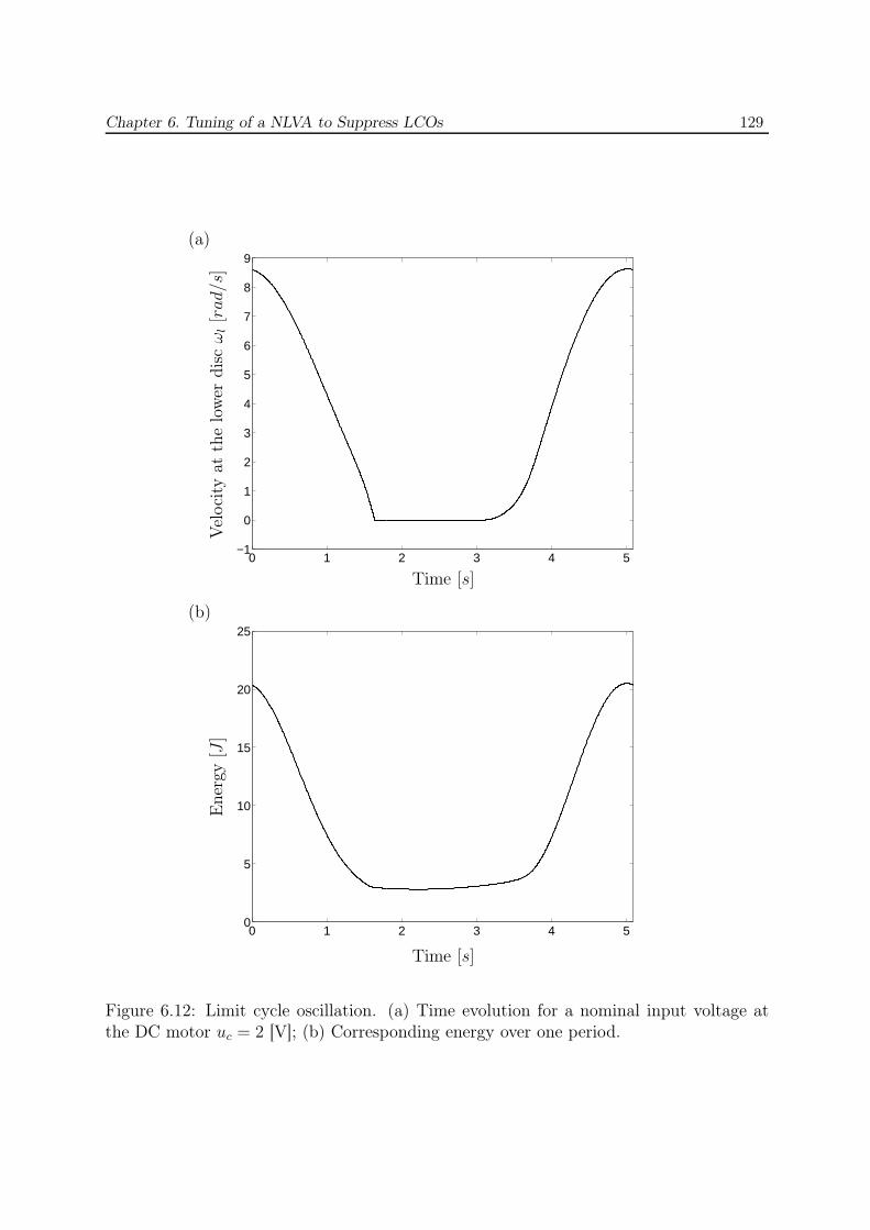
Chapter 6. Tuning of a NLVA to Suppress LCOs 129
0 1 2 3 4 5−1
0
1
2
3
4
5
6
7
8
9
0 1 2 3 4 50
5
10
15
20
25
Time [s]
Vel
oci
tyat
the
low
erdis
cω
l[r
ad/s
]
(a)
Time [s]
Ener
gy[J
]
(b)
Figure 6.12: Limit cycle oscillation. (a) Time evolution for a nominal input voltage atthe DC motor uc = 2 [V]; (b) Corresponding energy over one period.
Chapter 6. Tuning of a NLVA to Suppress LCOs 130
0 0.5 1 1.5 2 2.5 3 3.5 4−2
0
2
4
6
8
10
12
14
10−2
10−1
100
101
102
0.2
0.4
0.6
0.8
1
1.2
1.4
1.6
Input Voltage at the DC motor : u [V ]
Vel
oci
tyat
the
low
erdis
cω
l[r
ad/s
]
(a)
Energy [log]
Puls
atio
n[r
ad/s
]
(b)
α
α
β
β
β
Figure 6.13: Frequency-energy characterization of the drill-string system. (a) Bifurcationdiagram of the drill-string system with respect to the driving voltage uc, only the LCOlocus is represented (solid and dotted lines for stable and unstable solution, respectively);(b) Frequency-energy dependence of the LCOs, the solid, dash-dot and dashed lines cor-respond to the maximum, average and minimum of energy over one period. Finally, thedotted segments delimited by star corresponds to the energy information related to theunstable LCOs.

Chapter 7
Toward a Practical Realization of a
Nonlinear Vibration Absorber
Abstract
This chapter lays down the foundations of a practical realization of a nonlin-ear vibration absorber using nonlinear piezoelectric shunting. Specifically, theprinciple and theoretical bases on which the procedure relies are explained andapplied to a primary system consisting of a free vibrating beam. The dynamicscreated by the mechanical and electrical versions of the nonlinear vibrationabsorber are compared. Finally, future research directions are detailed.
131
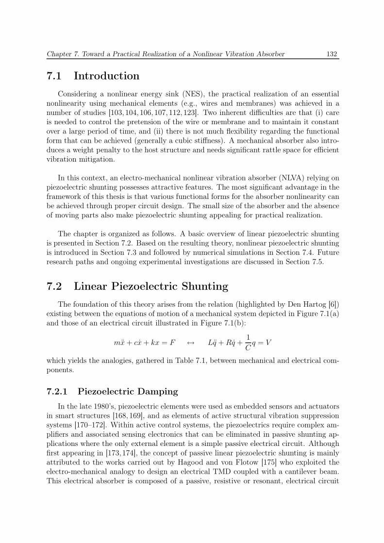
Chapter 7. Toward a Practical Realization of a Nonlinear Vibration Absorber 132
7.1 Introduction
Considering a nonlinear energy sink (NES), the practical realization of an essentialnonlinearity using mechanical elements (e.g., wires and membranes) was achieved in anumber of studies [103, 104, 106, 107, 112, 123]. Two inherent difficulties are that (i) careis needed to control the pretension of the wire or membrane and to maintain it constantover a large period of time, and (ii) there is not much flexibility regarding the functionalform that can be achieved (generally a cubic stiffness). A mechanical absorber also intro-duces a weight penalty to the host structure and needs significant rattle space for efficientvibration mitigation.
In this context, an electro-mechanical nonlinear vibration absorber (NLVA) relying onpiezoelectric shunting possesses attractive features. The most significant advantage in theframework of this thesis is that various functional forms for the absorber nonlinearity canbe achieved through proper circuit design. The small size of the absorber and the absenceof moving parts also make piezoelectric shunting appealing for practical realization.
The chapter is organized as follows. A basic overview of linear piezoelectric shuntingis presented in Section 7.2. Based on the resulting theory, nonlinear piezoelectric shuntingis introduced in Section 7.3 and followed by numerical simulations in Section 7.4. Futureresearch paths and ongoing experimental investigations are discussed in Section 7.5.
7.2 Linear Piezoelectric Shunting
The foundation of this theory arises from the relation (highlighted by Den Hartog [6])existing between the equations of motion of a mechanical system depicted in Figure 7.1(a)and those of an electrical circuit illustrated in Figure 7.1(b):
mx + cx + kx = F ↔ Lq + Rq +1
Cq = V
which yields the analogies, gathered in Table 7.1, between mechanical and electrical com-ponents.
7.2.1 Piezoelectric Damping
In the late 1980’s, piezoelectric elements were used as embedded sensors and actuatorsin smart structures [168, 169], and as elements of active structural vibration suppressionsystems [170–172]. Within active control systems, the piezoelectrics require complex am-plifiers and associated sensing electronics that can be eliminated in passive shunting ap-plications where the only external element is a simple passive electrical circuit. Althoughfirst appearing in [173,174], the concept of passive linear piezoelectric shunting is mainlyattributed to the works carried out by Hagood and von Flotow [175] who exploited theelectro-mechanical analogy to design an electrical TMD coupled with a cantilever beam.This electrical absorber is composed of a passive, resistive or resonant, electrical circuit
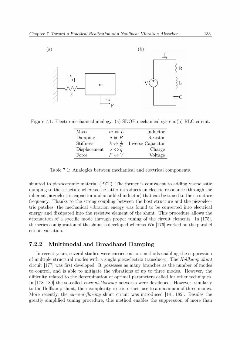
Chapter 7. Toward a Practical Realization of a Nonlinear Vibration Absorber 133
k
c
m
x
F
C
R
L
I
V
(a) (b)
Figure 7.1: Electro-mechanical analogy. (a) SDOF mechanical system;(b) RLC circuit.
Mass m ⇔ L InductorDamping c ⇔ R ResistorStiffness k ⇔ 1
CInverse Capacitor
Displacement x ⇔ q ChargeForce F ⇔ V Voltage
Table 7.1: Analogies between mechanical and electrical components.
shunted to piezoceramic material (PZT). The former is equivalent to adding viscoelasticdamping to the structure whereas the latter introduces an electric resonance (through theinherent piezoelectric capacitor and an added inductor) that can be tuned to the structurefrequency. Thanks to the strong coupling between the host structure and the piezoelec-tric patches, the mechanical vibration energy was found to be converted into electricalenergy and dissipated into the resistive element of the shunt. This procedure allows theattenuation of a specific mode through proper tuning of the circuit elements. In [175],the series configuration of the shunt is developed whereas Wu [176] worked on the parallelcircuit variation.
7.2.2 Multimodal and Broadband Damping
In recent years, several studies were carried out on methods enabling the suppressionof multiple structural modes with a single piezoelectric transducer. The Hollkamp shuntcircuit [177] was first developed. It possesses as many branches as the number of modesto control, and is able to mitigate the vibrations of up to three modes. However, thedifficulty related to the determination of optimal parameters called for other techniques.In [178–180] the so-called current-blocking networks were developed. However, similarlyto the Hollkamp shunt, their complexity restricts their use to a maximum of three modes.More recently, the current-flowing shunt circuit was introduced [181, 182]. Besides thegreatly simplified tuning procedure, this method enables the suppression of more than
Chapter 7. Toward a Practical Realization of a Nonlinear Vibration Absorber 134
three modes, simultaneously.
The aforementioned multimodal damping methods are characterized by an increasingcomplexity of the electrical scheme with the number of modes to be damped out. Thisfeature limits their application to a couple of modes and called for the introduction ofbroadband damping procedures. Therefore, the use of resistive damping [175], negativecapacitor [183–185] or periodic array of piezoelectric patches [186–188] was investigated.Although these solutions are of interest in many cases, they also possess drawbacks. In-deed, the first one presents limited effects whereas the two others are characterized by theloss of the passive properties and the need for multiple piezoelectric elements and shunts,respectively.
The validation of experimental results on continuous structures such as beams or platesrequire numerical simulations. These are carried out using a finite element formulation ofthe electro-mechanical system, which is described in the next section.
7.2.3 Finite Element Formulation
In [189], Allik et al. discretized the equations of motion of the electro-mechanicalsystem using a variational principle :
Muuδ + Kuuδ + Kuφφ = f (7.1)
Kφuδ + Kφφφ = q
where δ and φ are the displacements and voltages submitted to the piezoelectric element,respectively. Matrices Muu, Kuu, Kuφ (= KT
φu), Kφφ are, the structural mass, structuralstiffness, coupling, and the electrical matrices computed through the use of given shapefunctions and interpolation matrices, respectively.
Let us assume that the voltage varies harmonically with a frequency ω, φ = φ0eiωt,
then Equations (7.1) can be recast into :
[Kuu − ω2Muu + SZe(ω)] δ0 = f0, (7.2)
with the shunting matrix
SZe(ω) = −iωKuφ
(
iωKφφ −1
Ze(ω)
)−1
Kφu, (7.3)
Equations (7.2) and (7.3) govern the whole dynamics of the electro-mechanical system aslong as the compounds elements keep behaving in a linear fashion, enabling an algebraicresolution. Moreover, the impedance Ze(ω) gathers all the electrical effects arising fromthe shunt, for the methods presented in Sections 7.2.1 and 7.2.2.

Chapter 7. Toward a Practical Realization of a Nonlinear Vibration Absorber 135
7.3 Nonlinear Piezoelectric Shunting
In addition to the necessity of realizing a practical NLVA, the drawbacks related tolinear multimodal and broadband damping techniques (complexity of electrical scheme,multiple piezoelectric patches and shunts, energy supply) speak in favor of the develop-ment of new techniques such as the electrical NLVAs.
In particular, one of the main limitations occurs when attempting to damp out low fre-quency modes with small piezoelectric capacitor. In this case, the need for inductors withvalues greater than 1000 Henries may be required whereas the largest physical inductanceavailable today is approximatively 1 Henry. Therefore, virtual inductors were developedin [190] using differential amplifiers. In this context, the first nonlinear shunts were devel-oped. Some attempts focused on the possibility to alleviate the need for large inductorsusing the so-called switched shunt of switched stiffness (nonlinear) techniques [191–193].However, these techniques are not passive as an energy supply is required, and are, there-fore, classified as semi-active nonlinear methods.
Finally, in [194], the possibility to use nonlinear piezoelectric shunting for structuraldamping was investigated. The shunting components may be realized to allow the vibra-tional energy removed from the structure to be recovered in a usable form. The shuntingcircuits examined in this work are a rectified DC voltage source and a time-varying re-sistor. The study focused on the achievable damping levels, amplitude dependence, andpotential undesirable motions induced at higher harmonics of resonance or disturbancefrequencies by the electrical nonlinearities.
7.3.1 Basics
The developments carried out in the previous chapters focused on elastic nonlinearities.In particular, the case of an essentially nonlinear vibration absorber, depicted in Figure7.2 (a), was investigated. Its equation of motion, when acting alone, is given by :
mx + cx + knlx3 = F (7.4)
The electro-mechanical analogy presented in Section 7.2 suggests that the governing equa-tion of the analogous electrical circuit is expressed by :
Lq + Rq +1
Cnl
q3 = V (7.5)
which, therefore, imposes the presence of a nonlinear capacitor within the circuit, asdepicted in Figure 7.2 (b). Now, the study of a NLVA using nonlinear piezoelectricshunting can be carried out by first modeling the resulting electro-mechanical system.
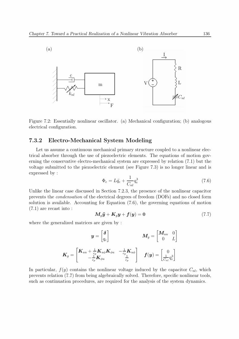
Chapter 7. Toward a Practical Realization of a Nonlinear Vibration Absorber 136
knl
c
m
x
F
Cnl
R
L
I
V
(a) (b)
Figure 7.2: Essentially nonlinear oscillator. (a) Mechanical configuration; (b) analogouselectrical configuration.
7.3.2 Electro-Mechanical System Modeling
Let us assume a continuous mechanical primary structure coupled to a nonlinear elec-trical absorber through the use of piezoelectric elements. The equations of motion gov-erning the conservative electro-mechanical system are expressed by relation (7.1) but thevoltage submitted to the piezoelectric element (see Figure 7.3) is no longer linear and isexpressed by :
Φe = Lqe +1
Cnl
q3e (7.6)
Unlike the linear case discussed in Section 7.2.3, the presence of the nonlinear capacitorprevents the condensation of the electrical degrees of freedom (DOFs) and no closed formsolution is available. Accounting for Equation (7.6), the governing equations of motion(7.1) are recast into :
Mgy + Kgy + f (y) = 0 (7.7)
where the generalized matrices are given by :
y =
[
δ
qe
]
Mg =
[
Muu 00 L
]
Kg =
[
Kuu + 1cp
KuφKφu − 1cp
Kuφ
− 1cp
Kφu1cp
]
f (y) =
[
01
Cnlq3e
]
In particular, f(y) contains the nonlinear voltage induced by the capacitor Cnl, whichprevents relation (7.7) from being algebraically solved. Therefore, specific nonlinear tools,such as continuation procedures, are required for the analysis of the system dynamics.
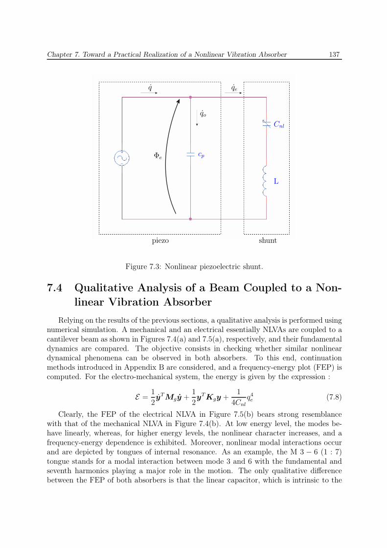
Chapter 7. Toward a Practical Realization of a Nonlinear Vibration Absorber 137
cp
Cnl
L
qeq
qo
Φe
piezo shunt
Figure 7.3: Nonlinear piezoelectric shunt.
7.4 Qualitative Analysis of a Beam Coupled to a Non-
linear Vibration Absorber
Relying on the results of the previous sections, a qualitative analysis is performed usingnumerical simulation. A mechanical and an electrical essentially NLVAs are coupled to acantilever beam as shown in Figures 7.4(a) and 7.5(a), respectively, and their fundamentaldynamics are compared. The objective consists in checking whether similar nonlineardynamical phenomena can be observed in both absorbers. To this end, continuationmethods introduced in Appendix B are considered, and a frequency-energy plot (FEP) iscomputed. For the electro-mechanical system, the energy is given by the expression :
E =1
2yTMgy +
1
2yTKgy +
1
4Cnl
q4e (7.8)
Clearly, the FEP of the electrical NLVA in Figure 7.5(b) bears strong resemblancewith that of the mechanical NLVA in Figure 7.4(b). At low energy level, the modes be-have linearly, whereas, for higher energy levels, the nonlinear character increases, and afrequency-energy dependence is exhibited. Moreover, nonlinear modal interactions occurand are depicted by tongues of internal resonance. As an example, the M 3 − 6 (1 : 7)tongue stands for a modal interaction between mode 3 and 6 with the fundamental andseventh harmonics playing a major role in the motion. The only qualitative differencebetween the FEP of both absorbers is that the linear capacitor, which is intrinsic to the
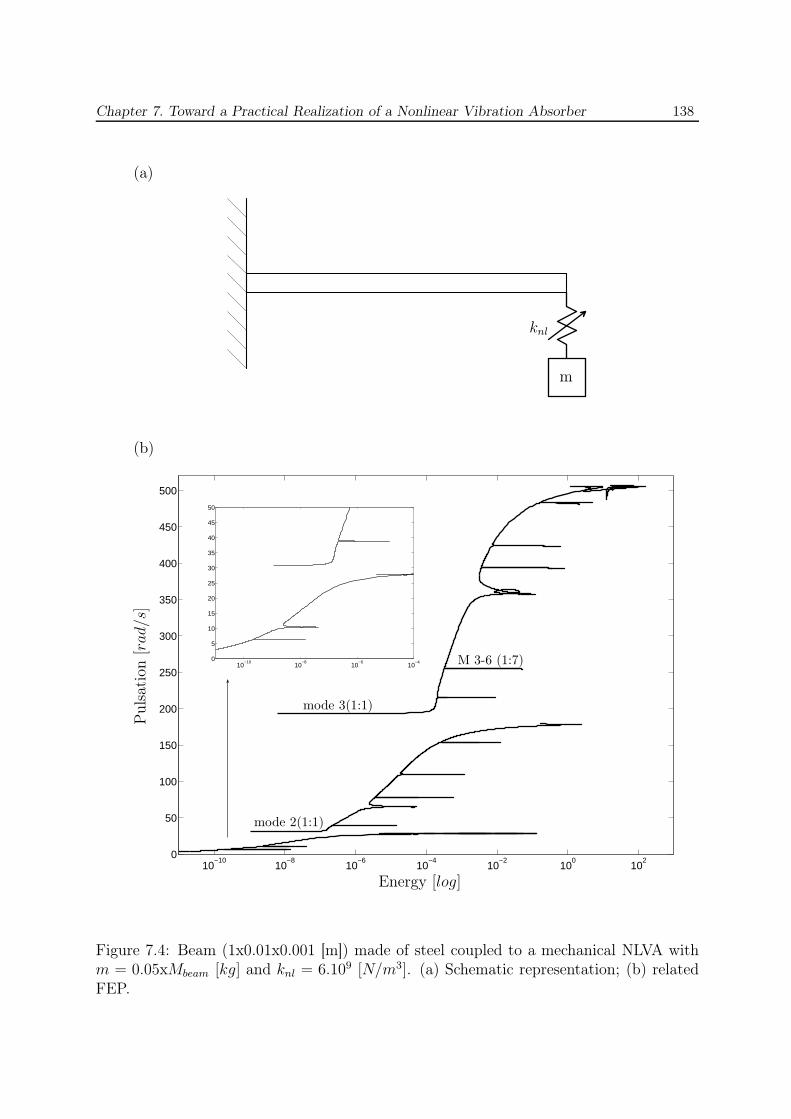
Chapter 7. Toward a Practical Realization of a Nonlinear Vibration Absorber 138
10−10
10−8
10−6
10−4
10−2
100
102
0
50
100
150
200
250
300
350
400
450
500
10−10
10−8
10−6
10−40
5
10
15
20
25
30
35
40
45
50
M 3-6 (1:7)
mode 2(1:1)
mode 3(1:1)
m
knl
(a)
(b)
Energy [log]
Puls
atio
n[r
ad/s
]
Figure 7.4: Beam (1x0.01x0.001 [m]) made of steel coupled to a mechanical NLVA withm = 0.05xMbeam [kg] and knl = 6.109 [N/m3]. (a) Schematic representation; (b) relatedFEP.
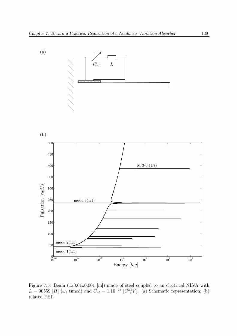
Chapter 7. Toward a Practical Realization of a Nonlinear Vibration Absorber 139
10−6
10−4
10−2
100
102
104
106
0
50
100
150
200
250
300
350
400
450
500
Cnl L
(a)
(b)
Energy [log]
Puls
atio
n[r
ad/s
]
mode 2(1:1)
mode 3(1:1)
mode 1(1:1)
M 3-6 (1:7)
Figure 7.5: Beam (1x0.01x0.001 [m]) made of steel coupled to an electrical NLVA withL = 90559 [H ] (ω1 tuned) and Cnl = 1.10−21 [C3/V ]. (a) Schematic representation; (b)related FEP.
Chapter 7. Toward a Practical Realization of a Nonlinear Vibration Absorber 140
piezoelectric element, introduces at low energy level a non-zero frequency for the firstmode.
In summary, it seems that it is possible to reproduce, using an electrical absorber, thedynamics created by an essentially nonlinear mechanical system, which paves the way fora practical realization of a NLVA.
7.5 Electrical Nonlinear Vibration Absorber Perspec-
tives
7.5.1 Short-Term Perspectives
7.5.1.1 Semi-Experimental Approach
A first step toward the practical realization of an electrical NLVA should rely on asemi-experimental approach. This consists in working directly on an experimental set-upwith a control law that mimics the electrical circuit. This is implemented numericallythanks to the use of a dedicated control software, dSPACE. This methodology is interest-ing for its flexibility; i.e., it enables straightforward modifications of the electrical circuit.
Figure 7.6 shows a schematic representation of the set-up. A source is applied at thefree end of the cantilever beam. One piezoelectric patch acts as a sensor; the associ-ated charge is converted by a charge amplifier, and the signal is injected in the dSPACEcontroller. The control law, initially created in Simulink, is imported in dSPACE andapplied to the incoming signal. The output signal passes through a voltage amplifier andis applied to an actuating piezoelectric patch. Finally, the beam response is measuredusing a laser vibrometer to avoid mass addition to the host structure.
A finite element model of the beam with piezoelectric elements can be created insoftware such as COMSOL and OOFELIE. The model can be reduced on specific DOFssuch as the potential on the piezoelectric electrodes and the DOFs at the beam end.A state-space formulation of the reduced model can then be injected into the Simulinkmodel, so that numerical validation of the semi-experimental set-up can be performed.
7.5.1.2 Essentially Nonlinear Piezoelectric Shunting
Even though the NLVA proposed in this thesis is not necessarily essentially nonlinear,the presence of the inherent capacitance of the piezoelectric element may complicate therealization of an essentially nonlinear absorber, i.e. an NES. A possible solution to thisproblem would be to consider a negative capacitor.

Chapter 7. Toward a Practical Realization of a Nonlinear Vibration Absorber 141
Chargeamplifier
Voltageamplifier
dSPACECONTROLLER
Source
Measurement
q1
V2
Figure 7.6: Schematic representation of the experimental setup.
7.5.2 Long-Term Perspectives
In addition to the aforementioned short-term perspectives, additional challenges shouldbe addressed to evolve toward a fully analogical piezoelectric shunt:
1. the optimization of the shape and localization of the piezoelectric elements;
2. the practical realization of the electrical components, namely a synthetic inductorand nonlinear capacitor;
3. the possible need of energy sources, such as operational amplifiers, to feed the syn-thetic elements;
4. the possibility to exploit energy harvesting to replace operational amplifiers.
The ultimate objective of this research should be to develop a nonlinear shunt incor-porated in a numerical chip.
7.6 Concluding Remarks
Realizing that a nonlinear absorber may be difficult to realize mechanically, the objec-tive of this chapter is to progress toward the development of an electrical absorber throughnonlinear piezoelectric shunting. The coupling of an electrical absorber to a cantilever

Chapter 7. Toward a Practical Realization of a Nonlinear Vibration Absorber 142
beam revealed that a dynamics similar to that of the same beam coupled to a mechanicalabsorber can be created. A number of short-term and long-term perspectives were alsoproposed for the continuation of this research work.
Conclusions
Nonlinear mechanical systems are characterized by the frequency-energy dependenceof their oscillations. This renders their vibration control and, hence, the design of non-linear vibration absorbers (NLVAs) challenging. In this context, the objective of thisdoctoral dissertation is to mitigate the vibrations of nonlinear mechanical systems usingNLVAs.
The first contribution of this thesis is to develop an absorber which can mitigate thevibrations of a nonlinear system in a wide range of input energies. Based on the resultsin Chapters 2 and 3, we showed that the backbone of the absorber should possess a quali-tatively similar dependence on energy as that of the backbone of the primary system. Tofulfill this frequency-energy-based tuning condition, the functional form of the absorbernonlinearity is to be carefully selected, which is an important result of this research work.
A departure from an absorber with essential nonlinearity, which was the starting pointof this thesis, was therefore necessary. Chapter 4 highlighted that, due to the existence ofenergy-invariant (fundamental and internally resonant) nonlinear normal modes, targetedenergy transfer from the primary structure to the NLVA can no longer be observed. Toour knowledge, it is also the first time that energy-invariant internally resonant nonlinearnormal modes are evidenced in a nonlinear system.
In addition to the qualitative tuning procedure, a quantitative methodology was pro-posed in Chapter 5, which targets the computation of adequate values for the absorbernonlinear coefficient and damping. To this end, the forced response was considered, andbifurcation analysis was exploited. Specifically, bifurcation tracking in parameter spacewas shown to be an effective alternative to computationally intensive parametric studies,and its use for NLVA tuning is another contribution of this thesis. Chapter 5 ended byproposing an integrated tuning procedure of a NLVA, which can deal with both free andforced vibration. Indeed, the underlying Hamiltonian dynamics drives the forced damped,dynamics, an assumption considered throughout this dissertation.
The possibility to extend the tuning methodology to primary systems presenting non-linear damping was investigated in Chapter 6. In this context, the suppression of the limitcycle oscillations of a drill-string system was considered. Assuming an essential nonlinear-ity for the absorber, adequate absorber parameters could be computed using bifurcationtracking, which substantially enlarged the domain of operation of the drill-string system.
143
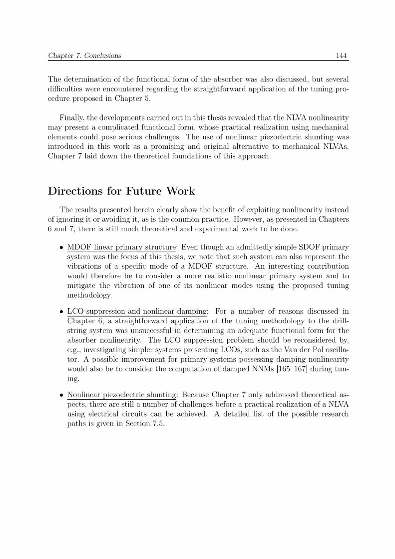
Chapter 7. Conclusions 144
The determination of the functional form of the absorber was also discussed, but severaldifficulties were encountered regarding the straightforward application of the tuning pro-cedure proposed in Chapter 5.
Finally, the developments carried out in this thesis revealed that the NLVA nonlinearitymay present a complicated functional form, whose practical realization using mechanicalelements could pose serious challenges. The use of nonlinear piezoelectric shunting wasintroduced in this work as a promising and original alternative to mechanical NLVAs.Chapter 7 laid down the theoretical foundations of this approach.
Directions for Future Work
The results presented herein clearly show the benefit of exploiting nonlinearity insteadof ignoring it or avoiding it, as is the common practice. However, as presented in Chapters6 and 7, there is still much theoretical and experimental work to be done.
• MDOF linear primary structure: Even though an admittedly simple SDOF primarysystem was the focus of this thesis, we note that such system can also represent thevibrations of a specific mode of a MDOF structure. An interesting contributionwould therefore be to consider a more realistic nonlinear primary system and tomitigate the vibration of one of its nonlinear modes using the proposed tuningmethodology.
• LCO suppression and nonlinear damping: For a number of reasons discussed inChapter 6, a straightforward application of the tuning methodology to the drill-string system was unsuccessful in determining an adequate functional form for theabsorber nonlinearity. The LCO suppression problem should be reconsidered by,e.g., investigating simpler systems presenting LCOs, such as the Van der Pol oscilla-tor. A possible improvement for primary systems possessing damping nonlinearitywould also be to consider the computation of damped NNMs [165–167] during tun-ing.
• Nonlinear piezoelectric shunting: Because Chapter 7 only addressed theoretical as-pects, there are still a number of challenges before a practical realization of a NLVAusing electrical circuits can be achieved. A detailed list of the possible researchpaths is given in Section 7.5.
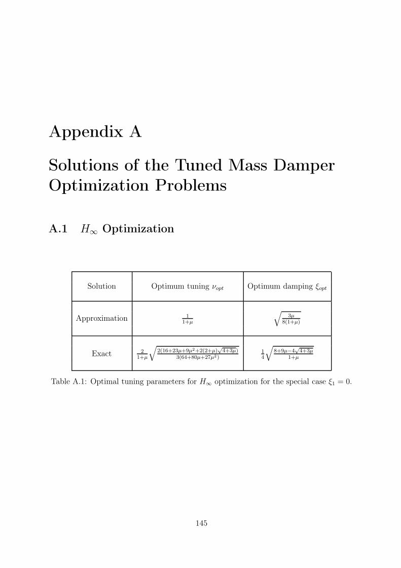
Appendix A
Solutions of the Tuned Mass Damper
Optimization Problems
A.1 H∞ Optimization
Solution Optimum tuning νopt Optimum damping ξopt
Approximation 11+µ
√
3µ8(1+µ)
Exact 21+µ
√
2(16+23µ+9µ2+2(2+µ)√
4+3µ)3(64+80µ+27µ2)
14
√
8+9µ−4√
4+3µ1+µ
Table A.1: Optimal tuning parameters for H∞ optimization for the special case ξ1 = 0.
145
Appendix A. Solutions of the Tuned Mass Damper Optimization Problems 146
Parameter νopt ξopt
SeriesSolution
11+ν
−ξ1
11+ν
√
12(1+µ)
(3 + 4µ − AB2+µ
) +
ξ21
C0−4(5+2µ)AB4(1+µ)2(2+µ)(9+4µ)
√
3µ8(1+µ)
+
ξ160+63µ+16µ2−2(3+2µ)AB
8(1+µ)(2+µ)(9+4µ)+
ξ21
C1(A+B)√
2+µ+C2(A−B)√
µ
32(1+µ)(2+µ)2(9+4µ)3√
2µ(1+µ)
Constants
A =√
3(2 + µ) −√
µ(2 + µ), B =√
3(2 + µ) +√
µ(2 + µ)
Force Excitation Motion Excitation
C0 = 52 + 41µ + 8µ2
C1 = −1296 + 2124µ + 6509µ2 +5024µ3 + 1616µ4 + 192µ5
C2 = 48168 + 112887µ + 105907µ2 +49664µ3 + 11632µ4 + 1088µ5
C0 = 52 + 113µ + 76µ2 + 16µ3
C1 = −1296 + 2124µ + 7157µ2 +5924µ3 + 2032µ4 + 256µ5
C2 = 48168 + 105111µ + 91867µ2 +40172µ3 + 8784µ4 + 768µ5
Table A.2: Optimal tuning parameters for H∞ optimization for the general case ξ1 6= 0.
A.2 H2 Optimization
Optimum tuning νopt Optimum damping ξopt
11+µ
√
2+µµ
√
µ(4+3µ)8(1+µ)(2+µ)
Table A.3: Optimal tuning parameters for H2 optimization for the special case ξ1 = 0.
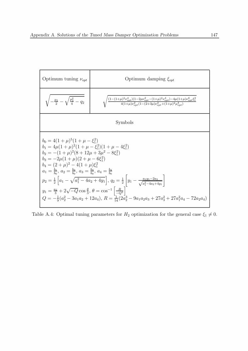
Appendix A. Solutions of the Tuned Mass Damper Optimization Problems 147
Optimum tuning νopt Optimum damping ξopt
√
−p2
2−
√
p22
4− q2
√
(1−(1+µ)2ν4opt)(1−2µν2
opt−(1+µ)2ν4opt)−4µ(1+µ)ν6
optξ21
4(1+µ)ν2opt(1−(2+3µ)ν2
opt+(1+µ)2µ4opt)
Symbols
b0 = 4(1 + µ)5(1 + µ − ξ21)
b1 = 4µ(1 + µ)2(1 + µ − ξ21)(1 + µ − 4ξ2
1)b2 = −(1 + µ)2(8 + 12µ + 3µ2 − 8ξ2
1)b3 = −2µ(1 + µ)(2 + µ − 6ξ2
1)b4 = (2 + µ)2 − 4(1 + µ)ξ2
1
a1 = b1b0
, a2 = b2b0
, a3 = b3b0
, a4 = b4b0
p2 = 12
[
a1 −√
a21 − 4a2 + 4y1
]
, q2 = 12
[
y1 − a1y1−2a3√a21−4a2+4y1
]
y1 = a2
3+ 2
√−Q cos θ3, θ = cos−1
[
R−Q3
]
Q = −19(a2
2 − 3a1a2 + 12a4), R = 154
(2a32 − 9a1a2a3 + 27a2
3 + 27a21a4 − 72a2a4)
Table A.4: Optimal tuning parameters for H2 optimization for the general case ξ1 6= 0.
Appendix B
Computation of Nonlinear Normal
Modes using Numerical Continuation
Compared to reference [109], a more robust and efficient algorithm for the NNMcomputation is utilized herein. This algorithm was first proposed in [129] and relies onthe combination of a shooting algorithm with pseudo-arclength continuation.
B.1 Shooting Method
The equations of motion of system (1.7) can be recast into state space form
x = f(x) (B.1)
where x is the state vector, and f is the vector field. The NNM computation is carried outby finding the periodic solutions of equations (B.1). In this context, the shooting methodsolves numerically the two-point boundary-value problem defined by the periodicity con-dition
H(xp0, T ) ≡ xp(T,xp0) − xp0 = 0 (B.2)
H(x0, T ) = x(T,x0) − x0 is called the shooting function and represents the differencebetween the initial conditions x0 and the system response at time T , x(T,x0). Starting
from some assumed initial conditions x(0)p0 , the motion x
(0)p (t,x
(0)p0 ) at the assumed period
T (0) can be obtained by numerical time integration methods (e.g., Runge-Kutta or New-
mark schemes). In general, the initial guess (x(0)p0 , T (0)) does not satisfy the periodicity
condition (B.2). A Newton-Raphson iteration scheme is therefore to be used to correct
an initial guess and to converge to the actual solution. The corrections ∆x(0)p0 and ∆T (0)
are found by expanding the nonlinear function
H(
x(0)p0 + ∆x
(0)p0 , T (0) + ∆T (0)
)
= 0 (B.3)
in Taylor series and neglecting higher-order terms.
148
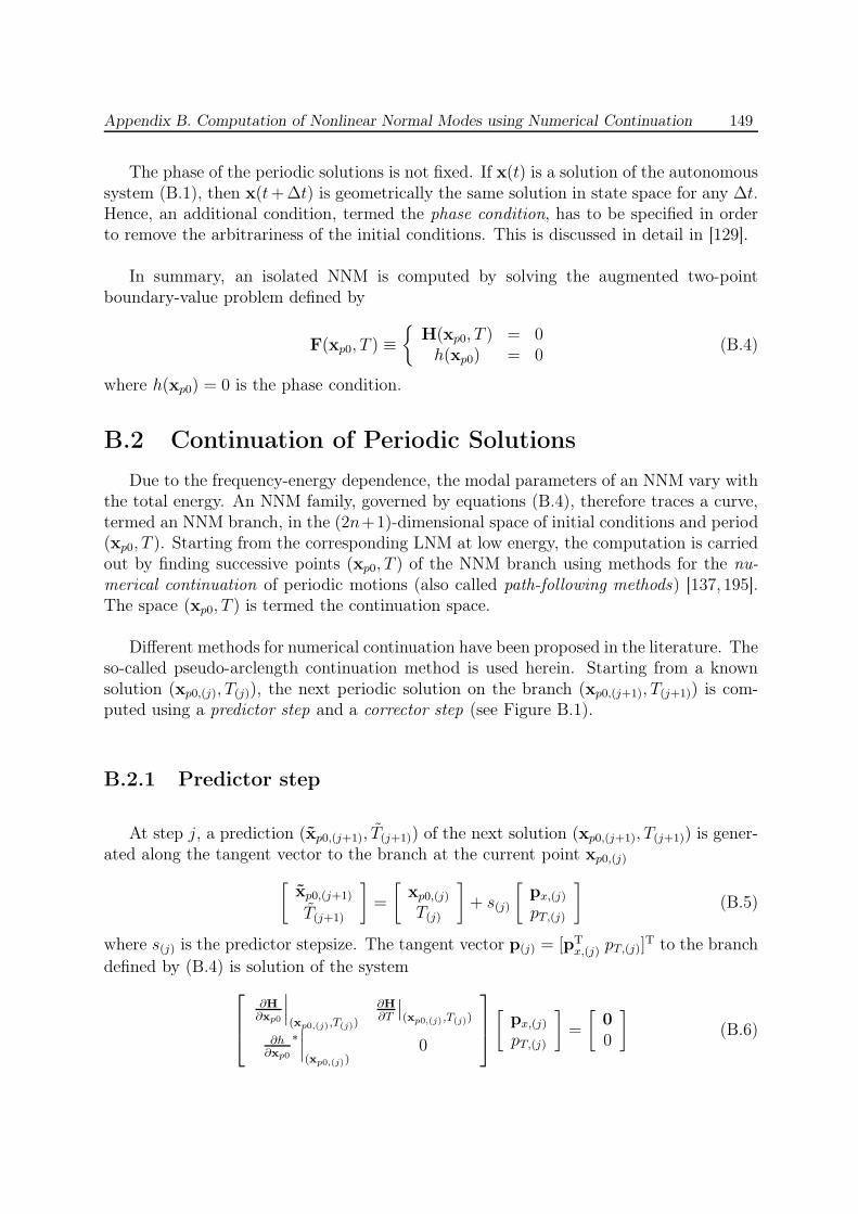
Appendix B. Computation of Nonlinear Normal Modes using Numerical Continuation 149
The phase of the periodic solutions is not fixed. If x(t) is a solution of the autonomoussystem (B.1), then x(t+∆t) is geometrically the same solution in state space for any ∆t.Hence, an additional condition, termed the phase condition, has to be specified in orderto remove the arbitrariness of the initial conditions. This is discussed in detail in [129].
In summary, an isolated NNM is computed by solving the augmented two-pointboundary-value problem defined by
F(xp0, T ) ≡{
H(xp0, T ) = 0h(xp0) = 0
(B.4)
where h(xp0) = 0 is the phase condition.
B.2 Continuation of Periodic Solutions
Due to the frequency-energy dependence, the modal parameters of an NNM vary withthe total energy. An NNM family, governed by equations (B.4), therefore traces a curve,termed an NNM branch, in the (2n+1)-dimensional space of initial conditions and period(xp0, T ). Starting from the corresponding LNM at low energy, the computation is carriedout by finding successive points (xp0, T ) of the NNM branch using methods for the nu-merical continuation of periodic motions (also called path-following methods) [137, 195].The space (xp0, T ) is termed the continuation space.
Different methods for numerical continuation have been proposed in the literature. Theso-called pseudo-arclength continuation method is used herein. Starting from a knownsolution (xp0,(j), T(j)), the next periodic solution on the branch (xp0,(j+1), T(j+1)) is com-puted using a predictor step and a corrector step (see Figure B.1).
B.2.1 Predictor step
At step j, a prediction (xp0,(j+1), T(j+1)) of the next solution (xp0,(j+1), T(j+1)) is gener-ated along the tangent vector to the branch at the current point xp0,(j)
[
xp0,(j+1)
T(j+1)
]
=
[
xp0,(j)
T(j)
]
+ s(j)
[
px,(j)
pT,(j)
]
(B.5)
where s(j) is the predictor stepsize. The tangent vector p(j) = [pTx,(j) pT,(j)]
T to the branch
defined by (B.4) is solution of the system
∂H
∂xp0
∣
∣
∣
(xp0,(j),T(j))
∂H
∂T
∣
∣
(xp0,(j) ,T(j))
∂h∂xp0
∗∣
∣
∣
(xp0,(j))0
[
px,(j)
pT,(j)
]
=
[
0
0
]
(B.6)
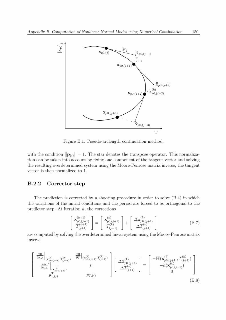
Appendix B. Computation of Nonlinear Normal Modes using Numerical Continuation 150
6
-T
[xp0] j
xp0,(j+1)
xp0,(j)
xp0,(j+2)
xp0,(j+3)
xp0,(j+1)
xp0,(j+2)
xp0,(j+3)
Pj
k
k + 1
x(k)p0,(j+2)
Figure B.1: Pseudo-arclength continuation method.
with the condition∥
∥p(j)
∥
∥ = 1. The star denotes the transpose operator. This normaliza-tion can be taken into account by fixing one component of the tangent vector and solvingthe resulting overdetermined system using the Moore-Penrose matrix inverse; the tangentvector is then normalized to 1.
B.2.2 Corrector step
The prediction is corrected by a shooting procedure in order to solve (B.4) in whichthe variations of the initial conditions and the period are forced to be orthogonal to thepredictor step. At iteration k, the corrections
[
x(k+1)p0,(j+1)
T(k+1)(j+1)
]
=
[
x(k)p0,(j+1)
T(k)(j+1)
]
+
[
∆x(k)p0,(j+1)
∆T(k)(j+1)
]
(B.7)
are computed by solving the overdetermined linear system using the Moore-Penrose matrixinverse
∂H
∂xp0
∣
∣
∣
(x(k)p0,(j+1)
,T(k)(j+1)
)
∂H
∂T
∣
∣
(x(k)p0,(j+1)
,T(k)(j+1)
)
∂h∂xp0
∗∣
∣
∣
(x(k)p0,(j+1)
)0
pTx,(j) pT,(j)
[
∆x(k)p0,(j+1)
∆T(k)(j+1)
]
=
−H(x(k)p0,(j+1), T
(k)(j+1))
−h(x(k)p0,(j+1))
0
(B.8)
Appendix B. Computation of Nonlinear Normal Modes using Numerical Continuation 151
where the prediction is used as initial guess, i.e, x(0)p0,(j+1) = xp0,(j+1) and T
(0)(j+1) = T(j+1).
The last equation in (B.8) corresponds to the orthogonality condition for the correctorstep.
This iterative process is carried out until convergence is achieved. The convergencetest is based on the relative error of the periodicity condition:
‖H(xp0, T )‖‖xp0‖
=‖xp(T,xp0) − xp0‖
‖xp0‖< ǫ (B.9)
where ǫ is the prescribed relative precision.
B.3 NNM Stability
The monodromy matrix being a by-product of the algorithm, the Floquet multipliers,and therefore the stability of the NNM motions, can be calculated in a straightforwardmanner [129].
Bibliography
[1] A. Preumont, Vibration Control of Active Structures : An introduction. KluwerAcademic Publishers, 1997.
[2] S. J. Dyke, B. F. Spencer, M. K. Sain, and J. D. Carlson, “Modeling and control ofmagnetorheological dampers for seismic response reduction,” Smart Materials andStructures, vol. 5, pp. 565–575, 1996.
[3] S. B. Choi and W. K. Kim, “Vibration control of a semi-active suspension featuringelectrorheological fluid dampers,” Journal of Sound and Vibration, vol. 234, pp. 537–546, 2000.
[4] B. C. Nakra, “Vibration control in machines and structures using viscoelastic damp-ing,” Journal of Sound and Vibration, vol. 211, pp. 449–465, 1998.
[5] H. Frahm, A Device for Damping Vibrations of Bodies. US Patent 989958, 1911.
[6] J. P. Den Hartog, Mechanical Vibrations. Dover Books on Engineering, 4th ed.,1985.
[7] J. Ormondroyd and J. P. Den Hartog, “The theory of the dynamical vibrationabsorber,” ASME Journal of Applied Mechanics, vol. 50(7), pp. 9–22, 1928.
[8] E. Hahnkamm, “Die dämpfung von fundamentschwingungen bei veränderlicher er-regergrequenz,” Engineering Architecture, vol. 4, pp. 192–201, 1932.
[9] J. E. Brock, “A note on the damped vibration absorber,” ASME Journal of AppliedMechanics, vol. 13(4), p. A284, 1946.
[10] O. Nishihara and H. Matsuhisa, “Design and tuning of vibration control devicesvia stability criterion,” Japanese Society of Mechanical Engineering, vol. 97-10-1,pp. 165–168, 1997.
[11] E. Pennestri, “An application of chebyshev’s min-max criterion to the optimal designof a damped dynamic vibration absorber,” Journal of Sound and Vibration, vol. 217,pp. 757–765, 1998.
[12] A. Thompson, “Auxiliary mass throw in a tuned and damped vibration absorber,”Journal of Sound and Vibration, vol. 70, pp. 481–486, 1980.
152
BIBLIOGRAPHY 153
[13] A. G. Thompson, “Optimum tuning and damping of a dynamic vibration absorberapplied to a force excited and damped primary system,” Journal of Sound andVibration, vol. 77(3), pp. 403–415, 1981.
[14] T. Asami, “Optimum design of dynamic absorbers for a system subjected to randomexcitation,” Japanese Society of Mechanical Engineering, vol. 34(2), pp. 218–226,1991.
[15] T. Asami, O. Nishihara, and A. M. Baz, “Analytical solutions to H∞ and H2 opti-mization of dynamic vibration absorbers attached to damped linear systems,” Jour-nal of Vibration and Acoustics, Transactions of the ASME, vol. 124, pp. 284–295,2002.
[16] Y. Fujino and M. Abe, “Design formulas for tuned mass dampers based on a per-turbation technique,” Earthquake Engineering and Structural Dynamics, vol. 22,pp. 833–854, 1993.
[17] H. Sekiguhi and T. Asami, “Theory of vibration isolation of a system with twodegrees of freedom,” Japanese Society of Mechanical Engineering, vol. 27-234,pp. 2839–2846, 1984.
[18] T. Asami and Y. Hosokawa, “Approximate expression for design of optimal dynamicabsorbers attached to damped linear systems (2nd report, optimization processbased on the fixed-points theory),” Japanese Society of Mechanical Engineering,vol. 61-583, pp. 915–921, 1995.
[19] Y. Iwata, “On the construction of the dynamic vibration absorbers,” Japanese So-ciety of Mechanical Engineering, vol. 820-8, pp. 150–152, 1982.
[20] I. N. Jordanov and B. I. Cheshankov, “Optimal design of linear and nonlinear dy-namical vibration absorbers,” Journal of Sound and Vibration, vol. 123, pp. 157–170,1988.
[21] I. N. Jordanov and B. I. Cheshankov, “Optimal design of linear and nonlineardynamical vibration absorbers, reply,” Journal of Sound and Vibration, vol. 132,pp. 157–159, 1989.
[22] S. H. Crandall and W. D. Mark, Random Vibration in Mechanical Systems. Aca-demic Press.
[23] T. Asami, K. Momose, and Y. Hosokawa, “Approximate expression for design ofoptimal dynamic absorbers attached to damped linear systems (optimization pro-cess based on the minimum variance criterion),” Japanese Society of MechanicalEngineering, vol. 59-566, pp. 2962–2967, 1993.
[24] H. Yamaguchi, “Damping transient vibration by a dynamic absorber,” JapaneseSociety of Mechanical Engineering, vol. 54-499, pp. 561–568, 1988.
BIBLIOGRAPHY 154
[25] O. Nishihara and H. Matsuhisa, “Design of a dynamic vibration absorber for mini-mization of maximum amplitude magnification factor (derivation of algebraic exactsolution),” Japanese Society of Mechanical Engineering, vol. 63-614, pp. 3438–3445,1997.
[26] K. Ikeda and T. Loi, “On the dynamic vibration damped absorber of the vibrationsystem,” Japanese Society of Mechanical Engineering, vol. 21-151, pp. 64–71, 1978.
[27] S. E. Randall, D. M. Halsted, and D. L. Taylor, “Optimum vibration absorbers forlinear damped systems,” ASME Journal of Mechanical Design, vol. 103-4, pp. 908–913, 1981.
[28] A. Soom and M. Lee, “Optimal design of linear and nonlinear vibration absorbers fordamped systems,” ASME Journal of Vibration and Acoustics, vol. 105-1, pp. 112–119, 1983.
[29] M. N. S. Hadi and Y. Arfiadi, “Optimum design of absorbers for MDOF structures,”Journal of Structural Engineering, vol. 124, pp. 1272–1280, 1998.
[30] M. P. Singh and L. M. Moreschi, “Optimal placement of dampers for passive responsecontrol,” Earthquake Engineering and Structural Dynamics, vol. 31, pp. 955–976,2002.
[31] R. Rana and T. T. Soong, “Parametric study and simplified design of tuned massdampers,” Engineering Structures, vol. 20, pp. 193–204, 1998.
[32] F. Sadek, B. Mohraz, A. W. Taylor, and R. M. Chung, “A method of estimatingthe parameters of tuned mass dampers for seismic applications,” Earthquake Engi-neering and Structural Dynamics, vol. 26, pp. 617–635, 1997.
[33] A. F. Vakakis and S. A. Paipetis, “The effect of a viscously damped dynamic ab-sorber on a linear multi-degree-of-freedom system,” Journal of Sound and Vibration,vol. 105, pp. 49–60, 1986.
[34] W. M. Haddad and A. Razavi, “H2, mixed H2/H∞, H2/L1 optimally tuned passiveisolators and absorbers,” ASME Journal of Dynamic Systems, Measurement, andControl, vol. 120, pp. 282–287, 1998.
[35] D. J. Stech, “H2 approach for optimally tuning passive vibration absorbers to flexiblestructures,” Journal of Guidance, Control and Dynamics, vol. 17, pp. 636–638, 1994.
[36] M. B. Ozer and T. J. Royston, “Application of Sherman-Morrison matrix inver-sion formula to damped vibration absorbers attached to multi-degree-of-freedomsystems,” Journal of Sound and Vibration, vol. 283, pp. 1235–1249, 2005.
[37] J. Sherman and W. J. Morrison, “Adjustment of an inverse matrix correspondingto changes in the elements of a given column of a given row of the original matrix,”Annals of Mathematical Statistics, vol. 20, p. 621, 1949.
BIBLIOGRAPHY 155
[38] W. W. Hager, “Updating the inverse of a matrix,” Society for Industrial and AppliedMathematics Review, vol. 31, pp. 221–239, 1989.
[39] H. Yamaguchi and N. Hampornchai, “Fundamental characteristics of multiple tunedmass dampers for suppressing harmonically forced oscillations,” Earthquake Engi-neering and Structural Dynamics, vol. 22, pp. 51–62, 1993.
[40] M. Abe and Y. Fujino, “Dynamic characteriszation of multiple tuned mass dampersand some design forumlas,” Earthquake Engineering and Structural Dynamics,vol. 23, pp. 813–835, 1994.
[41] K. Xu and T. Igusa, “Vibration control using multiple tuned mass dampers,” Journalof Sound and Vibration, vol. 175, pp. 491–503, 1994.
[42] A. Kareem and S. Kline, “Performance of multiple mass dampers under randomloading,” Journal of Structural Engineering ASCE, vol. 121, pp. 348–361, 1995.
[43] R. S. Jangid, “Dynamic characteristics of structures with multiple tuned massdampers,” Journal of Structural Engineering and Mechanics, vol. 3, pp. 497–509,1995.
[44] C. Li, “Performance of multiple tuned mass dampers for attenuating undesirableoscillations of structures under the ground acceleration,” Earthquake Engineeringand Structural Dynamics, vol. 29, pp. 1405–1421, 2000.
[45] Y. Q. Guo and W. Q. Chen, “Dynamic analysis of space structures with multipletuned mass dampers,” Engineering Structures, vol. 29, pp. 3390–3403, 2007.
[46] A. M. Kaynia, D. Veneziano, and J. M. Biggs, “Seismic effectiveness of tuned massdampers,” Journal of Structural Engineering, vol. 107(8), pp. 1465–1484, 1981.
[47] J. R. Sladek and R. E. Klingner, “Effect of tuned mass dampers on seismic response,”Journal of the Structural Division, vol. 109, pp. 2004–2009, 1983.
[48] A. H. Chowdhury, M. D. Iwuchukwu, and J. J. Garske, “Past and future of seismiceffectiveness of tuned mass dampers,” Proceedings of the 2nd International Sympo-sium on Structural Control, Ontario, Canada, pp. 105–127, 1985.
[49] R. Soto-Brito and S. E. Ruiz, “Influence of ground motion intensity on the effective-ness of tuned mass dampers,” Earthquake Engineering and Structural Dynamics,vol. 28, pp. 1255–1271, 1999.
[50] P. Lukkunaprasit and A. Wanitkorkul, “Inelastic buildings with tuned mass dampersunder moderate ground motions from distant earthquakes,” Earthquake Engineeringand Structural Dynamics, vol. 30(4), pp. 537–551, 2001.
[51] T. Pinkaew, P. Lukkunaprasit, and P. Chatupote, “Seismic effectiveness ot tunedmass dampers for damage reduction of structures,” Engineering Structures, vol. 25,pp. 39–46, 2003.
BIBLIOGRAPHY 156
[52] K. K. F. Wong and Y. L. Chee, “Energy dissipation of tuned mass dampers duringearthquake excitations,” Structural Design of Tall and Special Buildings, vol. 13,pp. 105–121, 2004.
[53] J. C. Miranda, “On tuned mass dampers for reducing the seismic response of struc-tures,” Earthquake Engineering and Structural Dynamics, vol. 34(7), pp. 847–865,2005.
[54] K. K. F. Wong, “Seismic energy dissipation of inelastic structures with tuned massdampers,” Journal of Engineering Mechanics, vol. 134(2), 2008.
[55] K. K. F. Wong and J. Johnson, “Seismic energy dissipation of inelastic structureswith multiple TMD,” Journal of Engineering Mechanics, vol. 135(4), 2009.
[56] S. Sgobba and G. C. Marano, “Optimum design of linear tuned mass dampers forstructures with nonlinear behaviour,” Mechanical System and Signal Processing,vol. 24(6), pp. 1739–1755, 2010.
[57] M. D. Rowbottom, “The optimization of mechanical dampers to control self-excitedgalloping oscillations,” Journal of Sound and Vibration, vol. 75, pp. 559–576, 1981.
[58] Y. Fujino, P. Warnitchai, and M. Ito, “Suppression of galloping of brigdge towerusing tuned mass dampers,” Journal of the Faculty of Engineering, The Universityof Tokyo, vol. 38, pp. 49–73, 1985.
[59] M. Abdel-Rohman, “Design of tuned mass dampers for suppression of galloping intall prismatic structures,” Journal of Sound and Vibration, vol. 171, pp. 289–299,1994.
[60] V. Gatulli, F. Di Fabio, and A. Luongo, “One-to-one resonant double Hopf bifur-cation in aeroelastic oscillators with tuned mass dampers,” Journal of Sound andVibration, vol. 262, pp. 201–217, 2003.
[61] R. E. Roberson, “Synthesis of a nonlinear dynamic vibration absorber,” Journal ofthe Franklin Institute, vol. 254, pp. 205–220, 1952.
[62] L. A. Pipes, “Analysis of a nonlinear dynamic vibration absorber,” Journal of Ap-plied Mechanics, vol. 20, pp. 515–518, 1953.
[63] F. R. Arnold, “Steady-state behavior of systems provided with nonlinear dynamicvibration absorbers,” Journal of Applied Mechanics, vol. 22, pp. 487–492, 1955.
[64] J. B. Hunt and J.-C. Nissen, “The broadband dynamic vibration absorber,” Journalof Sound and Vibration, vol. 83, pp. 573–578, 1982.
[65] J. P. Den Hartog, Tuned pendulums as torsional vibration eliminators. 1938.
[66] D. Newland, “Nonlinear aspects of the performance of centrifugal pendulum vibra-tion absorbers,” Journal of Engineering for Industry, vol. 86, pp. 257–263, 1964.
BIBLIOGRAPHY 157
[67] J. Madden, Constant frequency bifilar vibration absorber. US Patent 4218187, 1980.
[68] H. H. Denman, “Tautochronic bifilar pendulum torsion absorbers for reciprocatingengines,” Journal of Sound and Vibration, vol. 159, pp. 251–277, 1992.
[69] S. W. Shaw, P. M. Schmitz, and A. G. Haddow, “Dynamics of tautochronic pendu-lum vibration absorbers : Theory and experiment,” Journal of Computational andNonlinear Dynamics, vol. 1, pp. 283–293, 2006.
[70] C. P. Chao, C. T. Lee, and S. W. Shaw, “Non-unison dynamics of multiple centrifugalpendulum vibration absorbers,” Journal of Sound and Vibration, vol. 204, pp. 769–794, 1997.
[71] A. S. Alsuwaiyan and S. W. Shaw, “Performance and dynamic stability of general-path centrifugal pendulum vibration absorbers,” Journal of Sound and Vibration,vol. 252, pp. 791–815, 2002.
[72] T. M. Nester, A. G. Haddow, and S. W. Shaw, “Experimental investigation of asystem with nearly identical centrifugal pendulum vibration absorbers,” in Proceed-ings of the ASME 19th Biennal Conference on Mechanical Vibration and Noise,Chicago, Illinois, 2003.
[73] S. W. Shaw and C. Pierre, “The dynamic response of tuned impact absorbers forrotating flexible structures,” Journal of Computational and Nonlinear Dynamics,vol. 1, pp. 13–24, 2006.
[74] Y. Ishida, T. Inoue, T. Kagaw, and M. Ueda, “Nonlinear analysis of a torsionalvibration of a rotor with centrifugal pendulum vibration absorbers and its suppres-sion,” Japan Society of Mechanical Engineers, vol. C71, pp. 2431–2438, 2005.
[75] T. M. Nester, A. G. Haddow, S. W. Shaw, J. E. Brevick, and V. J. Borowski,“Vibration reduction in variable displacement engines using pendulum absorbers,”in Proceedings of the SAE Noise and Vibration Conference and Exhibition no 2003-01-1484, 2004.
[76] P. Lieber and D. Jensen, “An acceleration damper : development, design and someapplications,” ASME Transactions, vol. 67, pp. 523–530, 1945.
[77] S. F. Masri and T. K. Caughey, “On the stability of the impact damper,” Journalof Applied Mechanics, vol. 88, pp. 586–592, 1966.
[78] F. Peterka, “Bifurcations and transition phenomena in an impact oscillator,” Chaos,Solitons & Fractals, vol. 7, pp. 1635–1647, 1996.
[79] R. S. Haxton and A. D. S. Barr, “The autoparametric vibration absorber,” ASMEJournal of Engineering for Industry, vol. 94, pp. 119–125, 1972.
BIBLIOGRAPHY 158
[80] S. W. Shaw and B. Balachandran, “A review of nonlinear dynamics of mechanicalsystems in year 2008,” Journal of System Design and Dynamics, vol. 2, pp. 611–640,2008.
[81] A. Vyas and A. K. Bajaj, “Dynamics of autoparametric vibration absorbers usingmultiple pendulums,” Journal of Sound and Vibration, vol. 246, pp. 115–135, 2001.
[82] A. K. Bajaj, A. Vyas, and A. Raman, “Explorations into the nonlinear dynamics ofa single-degree-of-freedom system coupled to a wideband autoparametric vibrationabsorber,” Chaotic Dynamics and Control of Systems and Processes in Mechanics,pp. 17–26, 2005.
[83] A. H. Nayfeh and D. T. Mook, Nonlinear Oscillations. New-York: Wiley-Interscience, 1995.
[84] A. G. Haddow and A. B. D. Mook, “Theoretical and experimental study of modalinteraction in a two-degree-of-freedom structure,” Journal of Sound and Vibration,vol. 97, pp. 451–473, 1984.
[85] M. F. Golnaraghi, “Vibration suppression of flexible structures using internal reso-nance,” Mechanics Research Communications, vol. 18, pp. 135–143, 1991.
[86] M. P. Cartmell and J. W. Lawson, “Performance enhancement of an autoparametricvibration absorber by means of computer control,” Journal of Sound and Vibration,vol. 177, pp. 173–195, 1994.
[87] S. S. Oueini, A. H. Nayfeh, and M. F. Golnaraghi, “A theoretical and experimentalimplementation of a control method based on saturation,” Nonlinear Dynamics,vol. 13, pp. 189–202, 1997.
[88] S. S. Oueini, A. H. Nayfeh, and J. R. Pratt, “A nonlinear vibration absorber forflexible structures,” Nonlinear Dynamics, vol. 15, pp. 259–282, 1998.
[89] S. S. Oueini, A. H. Nayfeh, and J. R. Pratt, “A review of development and imple-mentation of an active nonlinear vibration absorber,” Archive of Applied Mechanics(Ingenieur Archiv), vol. 69, pp. 585–620, 1999.
[90] O. V. Gendelman, “Transition of energy to a nonlinear localized mode in a highlyasymmetric system of two oscillators,” Nonlinear dynamics, vol. 25, pp. 237–253,2001.
[91] O. V. Gendelman, L. I. Manevitch, A. F. Vakakis, and R. McCloskey, “Energypumping in nonlinear mechanical oscillators : part I - dynamics of the underlyinghamiltonian systems,” Journal of Applied Mechanics, vol. 68, pp. 34–41, 2001.
[92] A. F. Vakakis and O. V. Gendelman, “Energy pumping in nonlinear mechanicaloscillators : Part II - resonance capture,” Journal of Sound and Vibration, vol. 68,pp. 42–48, 2001.
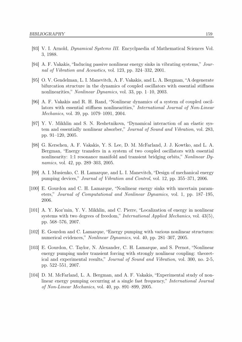
BIBLIOGRAPHY 159
[93] V. I. Arnold, Dynamical Systems III. Encyclpaedia of Mathematical Sciences Vol.3, 1988.
[94] A. F. Vakakis, “Inducing passive nonlinear energy sinks in vibrating systems,” Jour-nal of Vibration and Acoustics, vol. 123, pp. 324–332, 2001.
[95] O. V. Gendelman, L. I. Manevitch, A. F. Vakakis, and L. A. Bergman, “A degeneratebifurcation structure in the dynamics of coupled oscillators with essential stiffnessnonlinearities,” Nonlinear Dynamics, vol. 33, pp. 1–10, 2003.
[96] A. F. Vakakis and R. H. Rand, “Nonlinear dynamics of a system of coupled oscil-lators with essential stiffness nonlinearities,” International Journal of Non-LinearMechanics, vol. 39, pp. 1079–1091, 2004.
[97] Y. V. Mikhlin and S. N. Reshetnikova, “Dynamical interaction of an elastic sys-tem and essentially nonlinear absorber,” Journal of Sound and Vibration, vol. 283,pp. 91–120, 2005.
[98] G. Kerschen, A. F. Vakakis, Y. S. Lee, D. M. McFarland, J. J. Kowtko, and L. A.Bergman, “Energy transfers in a system of two coupled oscillators with essentialnonlinearity: 1:1 resonance manifold and transient bridging orbits,” Nonlinear Dy-namics, vol. 42, pp. 289–303, 2005.
[99] A. I. Musienko, C. H. Lamarque, and L. I. Manevitch, “Design of mechanical energypumping devices,” Journal of Vibration and Control, vol. 12, pp. 355–371, 2006.
[100] E. Gourdon and C. H. Lamarque, “Nonlinear energy sinks with uncertain param-eters,” Journal of Computational and Nonlinear Dynamics, vol. 1, pp. 187–195,2006.
[101] A. Y. Koz’min, Y. V. Mikhlin, and C. Pierre, “Localization of energy in nonlinearsystems with two degrees of freedom,” International Applied Mechanics, vol. 43(5),pp. 568–576, 2007.
[102] E. Gourdon and C. Lamarque, “Energy pumping with various nonlinear structures:numerical evidences,” Nonlinear Dynamics, vol. 40, pp. 281–307, 2005.
[103] E. Gourdon, C. Taylor, N. Alexander, C. H. Lamarque, and S. Pernot, “Nonlinearenergy pumping under transient forcing with strongly nonlinear coupling: theoret-ical and experimental results,” Journal of Sound and Vibration, vol. 300, no. 2-5,pp. 522–551, 2007.
[104] D. M. McFarland, L. A. Bergman, and A. F. Vakakis, “Experimental study of non-linear energy pumping occurring at a single fast frequency,” International Journalof Non-Linear Mechanics, vol. 40, pp. 891–899, 2005.
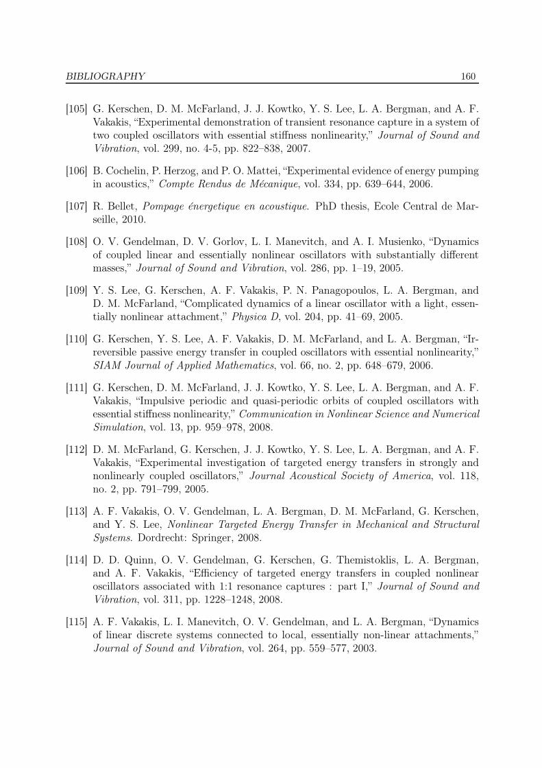
BIBLIOGRAPHY 160
[105] G. Kerschen, D. M. McFarland, J. J. Kowtko, Y. S. Lee, L. A. Bergman, and A. F.Vakakis, “Experimental demonstration of transient resonance capture in a system oftwo coupled oscillators with essential stiffness nonlinearity,” Journal of Sound andVibration, vol. 299, no. 4-5, pp. 822–838, 2007.
[106] B. Cochelin, P. Herzog, and P. O. Mattei, “Experimental evidence of energy pumpingin acoustics,” Compte Rendus de Mécanique, vol. 334, pp. 639–644, 2006.
[107] R. Bellet, Pompage énergetique en acoustique. PhD thesis, Ecole Central de Mar-seille, 2010.
[108] O. V. Gendelman, D. V. Gorlov, L. I. Manevitch, and A. I. Musienko, “Dynamicsof coupled linear and essentially nonlinear oscillators with substantially differentmasses,” Journal of Sound and Vibration, vol. 286, pp. 1–19, 2005.
[109] Y. S. Lee, G. Kerschen, A. F. Vakakis, P. N. Panagopoulos, L. A. Bergman, andD. M. McFarland, “Complicated dynamics of a linear oscillator with a light, essen-tially nonlinear attachment,” Physica D, vol. 204, pp. 41–69, 2005.
[110] G. Kerschen, Y. S. Lee, A. F. Vakakis, D. M. McFarland, and L. A. Bergman, “Ir-reversible passive energy transfer in coupled oscillators with essential nonlinearity,”SIAM Journal of Applied Mathematics, vol. 66, no. 2, pp. 648–679, 2006.
[111] G. Kerschen, D. M. McFarland, J. J. Kowtko, Y. S. Lee, L. A. Bergman, and A. F.Vakakis, “Impulsive periodic and quasi-periodic orbits of coupled oscillators withessential stiffness nonlinearity,” Communication in Nonlinear Science and NumericalSimulation, vol. 13, pp. 959–978, 2008.
[112] D. M. McFarland, G. Kerschen, J. J. Kowtko, Y. S. Lee, L. A. Bergman, and A. F.Vakakis, “Experimental investigation of targeted energy transfers in strongly andnonlinearly coupled oscillators,” Journal Acoustical Society of America, vol. 118,no. 2, pp. 791–799, 2005.
[113] A. F. Vakakis, O. V. Gendelman, L. A. Bergman, D. M. McFarland, G. Kerschen,and Y. S. Lee, Nonlinear Targeted Energy Transfer in Mechanical and StructuralSystems. Dordrecht: Springer, 2008.
[114] D. D. Quinn, O. V. Gendelman, G. Kerschen, G. Themistoklis, L. A. Bergman,and A. F. Vakakis, “Efficiency of targeted energy transfers in coupled nonlinearoscillators associated with 1:1 resonance captures : part I,” Journal of Sound andVibration, vol. 311, pp. 1228–1248, 2008.
[115] A. F. Vakakis, L. I. Manevitch, O. V. Gendelman, and L. A. Bergman, “Dynamicsof linear discrete systems connected to local, essentially non-linear attachments,”Journal of Sound and Vibration, vol. 264, pp. 559–577, 2003.
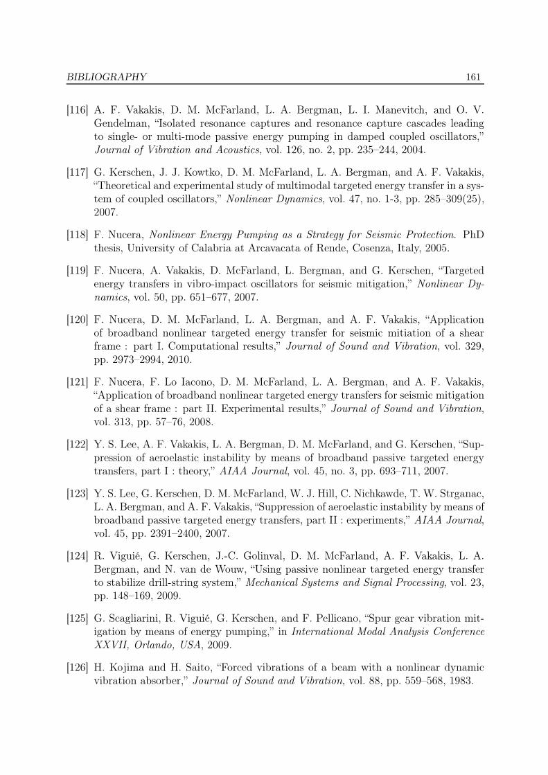
BIBLIOGRAPHY 161
[116] A. F. Vakakis, D. M. McFarland, L. A. Bergman, L. I. Manevitch, and O. V.Gendelman, “Isolated resonance captures and resonance capture cascades leadingto single- or multi-mode passive energy pumping in damped coupled oscillators,”Journal of Vibration and Acoustics, vol. 126, no. 2, pp. 235–244, 2004.
[117] G. Kerschen, J. J. Kowtko, D. M. McFarland, L. A. Bergman, and A. F. Vakakis,“Theoretical and experimental study of multimodal targeted energy transfer in a sys-tem of coupled oscillators,” Nonlinear Dynamics, vol. 47, no. 1-3, pp. 285–309(25),2007.
[118] F. Nucera, Nonlinear Energy Pumping as a Strategy for Seismic Protection. PhDthesis, University of Calabria at Arcavacata of Rende, Cosenza, Italy, 2005.
[119] F. Nucera, A. Vakakis, D. McFarland, L. Bergman, and G. Kerschen, “Targetedenergy transfers in vibro-impact oscillators for seismic mitigation,” Nonlinear Dy-namics, vol. 50, pp. 651–677, 2007.
[120] F. Nucera, D. M. McFarland, L. A. Bergman, and A. F. Vakakis, “Applicationof broadband nonlinear targeted energy transfer for seismic mitiation of a shearframe : part I. Computational results,” Journal of Sound and Vibration, vol. 329,pp. 2973–2994, 2010.
[121] F. Nucera, F. Lo Iacono, D. M. McFarland, L. A. Bergman, and A. F. Vakakis,“Application of broadband nonlinear targeted energy transfers for seismic mitigationof a shear frame : part II. Experimental results,” Journal of Sound and Vibration,vol. 313, pp. 57–76, 2008.
[122] Y. S. Lee, A. F. Vakakis, L. A. Bergman, D. M. McFarland, and G. Kerschen, “Sup-pression of aeroelastic instability by means of broadband passive targeted energytransfers, part I : theory,” AIAA Journal, vol. 45, no. 3, pp. 693–711, 2007.
[123] Y. S. Lee, G. Kerschen, D. M. McFarland, W. J. Hill, C. Nichkawde, T. W. Strganac,L. A. Bergman, and A. F. Vakakis, “Suppression of aeroelastic instability by means ofbroadband passive targeted energy transfers, part II : experiments,” AIAA Journal,vol. 45, pp. 2391–2400, 2007.
[124] R. Viguié, G. Kerschen, J.-C. Golinval, D. M. McFarland, A. F. Vakakis, L. A.Bergman, and N. van de Wouw, “Using passive nonlinear targeted energy transferto stabilize drill-string system,” Mechanical Systems and Signal Processing, vol. 23,pp. 148–169, 2009.
[125] G. Scagliarini, R. Viguié, G. Kerschen, and F. Pellicano, “Spur gear vibration mit-igation by means of energy pumping,” in International Modal Analysis ConferenceXXVII, Orlando, USA, 2009.
[126] H. Kojima and H. Saito, “Forced vibrations of a beam with a nonlinear dynamicvibration absorber,” Journal of Sound and Vibration, vol. 88, pp. 559–568, 1983.
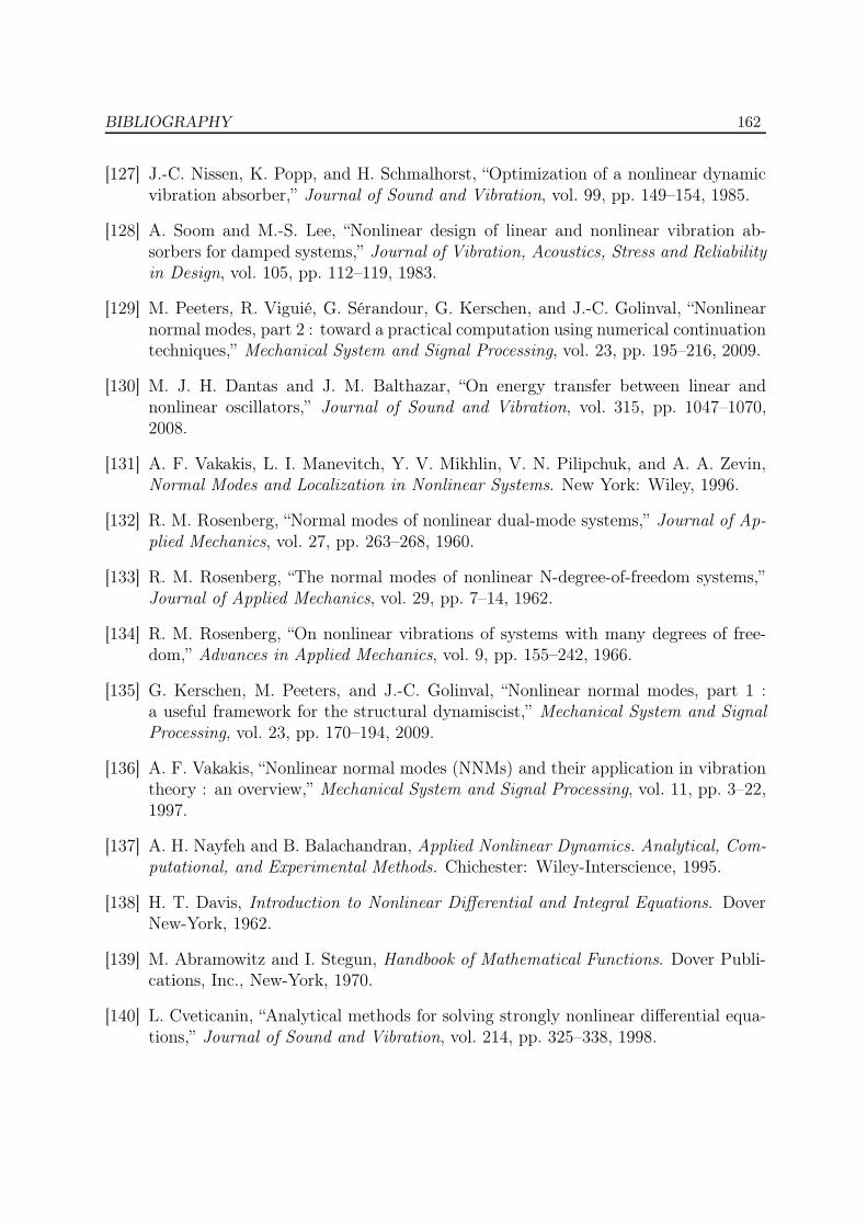
BIBLIOGRAPHY 162
[127] J.-C. Nissen, K. Popp, and H. Schmalhorst, “Optimization of a nonlinear dynamicvibration absorber,” Journal of Sound and Vibration, vol. 99, pp. 149–154, 1985.
[128] A. Soom and M.-S. Lee, “Nonlinear design of linear and nonlinear vibration ab-sorbers for damped systems,” Journal of Vibration, Acoustics, Stress and Reliabilityin Design, vol. 105, pp. 112–119, 1983.
[129] M. Peeters, R. Viguié, G. Sérandour, G. Kerschen, and J.-C. Golinval, “Nonlinearnormal modes, part 2 : toward a practical computation using numerical continuationtechniques,” Mechanical System and Signal Processing, vol. 23, pp. 195–216, 2009.
[130] M. J. H. Dantas and J. M. Balthazar, “On energy transfer between linear andnonlinear oscillators,” Journal of Sound and Vibration, vol. 315, pp. 1047–1070,2008.
[131] A. F. Vakakis, L. I. Manevitch, Y. V. Mikhlin, V. N. Pilipchuk, and A. A. Zevin,Normal Modes and Localization in Nonlinear Systems. New York: Wiley, 1996.
[132] R. M. Rosenberg, “Normal modes of nonlinear dual-mode systems,” Journal of Ap-plied Mechanics, vol. 27, pp. 263–268, 1960.
[133] R. M. Rosenberg, “The normal modes of nonlinear N-degree-of-freedom systems,”Journal of Applied Mechanics, vol. 29, pp. 7–14, 1962.
[134] R. M. Rosenberg, “On nonlinear vibrations of systems with many degrees of free-dom,” Advances in Applied Mechanics, vol. 9, pp. 155–242, 1966.
[135] G. Kerschen, M. Peeters, and J.-C. Golinval, “Nonlinear normal modes, part 1 :a useful framework for the structural dynamiscist,” Mechanical System and SignalProcessing, vol. 23, pp. 170–194, 2009.
[136] A. F. Vakakis, “Nonlinear normal modes (NNMs) and their application in vibrationtheory : an overview,” Mechanical System and Signal Processing, vol. 11, pp. 3–22,1997.
[137] A. H. Nayfeh and B. Balachandran, Applied Nonlinear Dynamics. Analytical, Com-putational, and Experimental Methods. Chichester: Wiley-Interscience, 1995.
[138] H. T. Davis, Introduction to Nonlinear Differential and Integral Equations. DoverNew-York, 1962.
[139] M. Abramowitz and I. Stegun, Handbook of Mathematical Functions. Dover Publi-cations, Inc., New-York, 1970.
[140] L. Cveticanin, “Analytical methods for solving strongly nonlinear differential equa-tions,” Journal of Sound and Vibration, vol. 214, pp. 325–338, 1998.
BIBLIOGRAPHY 163
[141] L. Cveticanin, “Analytical solutions of the system of two coupled pure cubic non-linear oscillators equations,” Journal Acoustical Society of America of Sound andVibration, vol. 245, pp. 571–580, 2001.
[142] L. Cveticanin, “The motion of a two-mass system with nonlinear connection,” Jour-nal of Sound and Vibration, vol. 252, pp. 361–369, 2002.
[143] L. Cveticanin, “Vibration of a coupled two-degree-of-freedom system,” Journal ofSound and Vibration, vol. 247, pp. 279–292, 2001.
[144] A. F. Vakakis, Analysis and Identification of Linear and Nonlinear Normal Modes.PhD thesis, California Institute of Technology, Pasadena, California, 1990.
[145] M. E. King and A. F. Vakakis, “An energy-based approach to computing resonantnonlinear normal modes,” Journal of Applied Mechanics, vol. 63, pp. 810–819, 1996.
[146] O. V. Gendelman, A. F. Vakakis, and G. Kerschen, “A degenerate bifurcation struc-ture in the dynamics of coupled oscillators with essential stiffness nonlinearities,”Nonlinear Dynamics, vol. 33, pp. 1–10, 2003.
[147] R. Viguié, M. Peeters, G. Kerschen, and J.-C. Golinval, “Energy transfer and dissi-pation in a duffing oscillator coupled to a nonlinear attachment,” Journal of Com-putational and Nonlinear Dynamics, vol. 4, pp. 041012–1/13, 2009.
[148] S. Tsakirtzis, P. N. Panagopoulos, G. Kerschen, O. V. Gendelman, A. F. Vakakis,and L. A. Bergman, “Complex dynamics and targeted energy transfer in linear oscil-lators coupled to multidegree-of-freedom essentially nonlinear attachments,” Non-linear Dynamics, vol. 48, pp. 285–318(34), May 2007.
[149] M. E. King and A. F. Vakakis, “An energy-based formulation for computing non-linear normal modes in undamped continuous systems,” Journal of Vibration andAcoustics, vol. 116, pp. 332–340, 1994.
[150] K. Jayaprakash, Y. Starosvetsky, A. Vakakis, M. Peeters, and G. Kerschen, “Non-linear normal modes and band zones in granular chains with no pre-compression,”Nonlinear Dynamics (In Review).
[151] E. Doedel, “Auto, software for continuation and bifurcation problems in ordinarydifferential equations (http://indy.cs.concordia.ca/auto/),”
[152] W. Govaerts, R. Khoshsiar Ghaziani, Y. Kuznetsov, and H. Meijer, “Matcont :A toolbox for continuation and bifurcation of cycles of maps,” Universiteit Gent(Belgium) - Utrecht University (The Netherlands), 2007.
[153] Y. A. Kuznetsov, Elements of Applied Bifurcation Theory. Science Press,1995,1998,2004.
[154] S. H. Strogatz, Nonlinear Dynamics and Chaos. Cambridge: Westview Press, 2000.
BIBLIOGRAPHY 164
[155] R. W. Bunton and C. M. Denegri, “Limit cycle oscillation characteristics of fighteraircraft,” Journal of Aircraft, vol. 37, pp. 916–918, 2000.
[156] R. A. Cunningham, “Analysis of downhole measurements of drill-string forces andmotions,” ASME Journal of Engineering for Industry, vol. 90, pp. 208–216, 1968.
[157] R. Leine, D. van Campen, and W. Keultjes, “Stick-slip whirl interaction in drill-string dynamics,” Journal of Vibration and Acoustics, vol. 124, pp. 209–220, 2002.
[158] J. F. Brett, “Genesis of torsional drill-string vibrations,” SPE Drilling Engineering,vol. 7, pp. 168–174, 1992.
[159] J. D. Jansen and L. van den Steen, “Active damping of self-excited torsional vibra-tions in oil well drill-string,” Journal of Sound and Vibration, vol. 179, pp. 647–668,1995.
[160] L. Van den Steen, Suppressing Stick-Slip-Induced Drill-string Oscillations : a HyperStability Approach. PhD thesis, |1997|.
[161] J. de Bruin, A. Doris, N. van de Wouw, W. W.P.M.H. Heemels, and H. Nijmei-jer, “Control of mechanical motion systems with non-collocation of actuation andfriction : A popov criterion approach for input-to-state stability and set-valuednonlinearities,” Automatica, vol. 45, pp. 409–415, 2009.
[162] C. Germay, Modeling and analysis of self-excited drill bit vibrations. PhD thesis,University of Liège, 2009.
[163] N. Mihajlovic, Torsional and Lateral Vibrations in Flexible Rotor Systems with Fric-tion. PhD thesis, 2005.
[164] N. Mihajlovic, N. V. de Wouw, M. P. M. Hendriks, and H. Nijmeijer, “Friction-induced limit cycling in flexible rotor systems and experimental drill-string set-up,”Nonlinear Dynamics, vol. 46, pp. 273–291, 2006.
[165] S. W. Shaw and C. Pierre, “Nonlinear normal modes and invariant manifolds,”Journal of Sound and Vibration, vol. 150, pp. 170–173, 1991.
[166] S. W. Shaw and C. Pierre, “On nonlinear normal modes,” ASME winter AnnualMeeting, 1992.
[167] S. W. Shaw and C. Pierre, “Normal modes for nonlinear vibratory systems,” Journalof Sound and Vibration, vol. 164, pp. 85–124, 1994.
[168] E. F. Crawley and J. DeLuis, “Use of piezoelectric actuators as elements of intelligentstructures,” American Institute of Aeronautics and Astronautics, vol. 25, pp. 1373–1385, 1987.
BIBLIOGRAPHY 165
[169] N. W. Hagood and E. F. Crawley, “Experimental investigation into passive dampingenhancement for space structures,” in Proceedings of AIAA Guidance Navigationand Control Conference, Boston, Massachusetts, 1989.
[170] J. L. Fanson and T. K. Caughey, “Positive position feedback control for large spacestructures,” American Institute of Aeronautics and Astronautics, vol. 28, pp. 717–724, 1990.
[171] S. Hanagud, M. W. Obal, and A. J. Calise, “Optimal vibration control bythe use of piezoceramic sensors and actuators,” in Proceedings of the 18thAIAA/ASME/ASCE/AHS Structures Structural Dyanmics and Materials Confer-ence, 1987.
[172] T. Bailey and J. E. Hubbard, “Distributed piezoelectric-polymer active vibrationcontrol of a cantilever beam,” American Institute of Aeronautics and AstronauticsJournal of Guidance Control and Dynamic, vol. 8, pp. 605–611, 1985.
[173] R. L. Forward, “Electronic damping of vibrations in optical structures,” Journal ofApplied Optics, vol. 18, pp. 690–697, 1979.
[174] R. L. Forward and C. J. Swigert, “Electronic damping of orthogonal bending modesin a cylindrical mast-theory,” Journal of Spacecraft and Rockets, vol. 18, pp. 5–10,1981.
[175] N. W. Hagood and A. von Flotow, “Damping of structural vibrations with piezo-electric materials and passive electrical networks,” Journal of Sound and Vibration,vol. 146, pp. 243–268, 1991.
[176] S. Y. Wu, “Piezoelectric shunts with parallel R-L circuit for smart structural damp-ing and vibration control,” in Proceedings SPIE : Smart Structure and Materials1996 : Passive Damping and Isolation, vol. 2720, pp. 259–269, 1996.
[177] J. J. Hollkamp, “Multimodal passive vibration suppression with piezoelectric mate-rials and resonant shunts,” Journal of Intelligent Material Systems and Structures,vol. 5, pp. 49–57, 1994.
[178] S. Y. Wu, “Method for multiple mode shunt damping of structural vibration usinga single PZT transducer,” in Proceedings SPIE Smart Structures and Materials,Smart Structures and Intelligent Systems, vol. 3327, pp. 159–168, 1998.
[179] S. Y. Wu, “Multiple PZT transducers implemented with multiple-mode piezoelectricshunting for passive vibration damping,” in Proceedings SPIE Smart Structures andMaterials, Passive Damping and Isolation, vol. 3672, pp. 112–122, 1999.
[180] S. Y. Wu and A. S. Bicos, “Structural vibration damping experiments using im-proved piezoelectric shunts,” in Proceedings SPIE, Smart Materials and Structures,Passive Damping and Isolation, vol. 3045, pp. 40–50, 1997.
BIBLIOGRAPHY 166
[181] S. Behrens, A. J. Fleming, and S. O. R. Moheimani, “New method for multiple-modeshunt damping of structural vibration using a single piezoelectric transducer,” inProceedings SPIE : Smart Structure and Materials : Passive Damping and Isolation,vol. 4331, pp. 230–250, 2001.
[182] S. Behrens, S. O. R. Moheimani, and A. J. Fleming, “Multiple mode current flowingpassive piezoelectric shunt controller,” Journal of Sound an Vibration, vol. 266,pp. 929–942, 2003.
[183] C. H. Park and A. Baz, “Vibration control of beams with negative capacitiveshunting of interdigital electrode piezoceramics,” Journal of Vibration and Control,vol. 11, pp. 311–346, 2005.
[184] S. Behrens, A. J. Fleming, and S. O. R. Moheimani, “A broadband controller forpiezoelectric shunt damping of structural vibration,” IOP Smart Materials andStructures, vol. 12, pp. 18–28, 2003.
[185] S. Y. Wu, Broadband piezoelectric shunts for structural vibration control. US Patent6.075.309, 2000.
[186] O. Thorp, M. Ruzzene, and A. Baz, “Attenuation and localization of waves in shellswith periodic shunted piezo rings,” Smart Materials and Structures, vol. 14, pp. 594–604, 2005.
[187] A. Spadoni, M. Ruzzene, and K. A. Cunefare, “Vibration and wave propagationcontrol of plates with periodic arrays of shunted piezoelectric patches,” in Proeedingsof ICAST Conference, 2007.
[188] M. Collet, K. A. Cunefare, and M. N. Ichchou, “Wave motion optimization in peri-odically distributed shunted piezocomposite beam structures,” Journal of intelligentmaterial systems and structures, vol. 20, pp. 787–808, 2009.
[189] H. Allik and T. J. R. Hughes, “Finite element method for piezoelectric vibration,”International Journal for Numerical Methods in Engineering, vol. 2, pp. 151–157,1970.
[190] R. H. S. Riordan, “Simulated inductors using differential amplifiers,” IEE ElectronicsLetters, vol. 3, pp. 50–51, 1967.
[191] L. R. Corr and W. W. Clark, “Comparison of low-frequency piezoelectric switchingshunt techniques for structural damping,” IOP Smart Materials and Structures,vol. 11, pp. 370–376, 2002.
[192] J. Ducarne, Modélisation et optimisation de dispositifs non-linéairesd’amortissement de structures par systèmes piézoélectriques commutés. PhDthesis, Conservatoire National des Arts et Métiers, Laboratoire de Mécanique desStructures et des Systèmes Couplés, 2009.

BIBLIOGRAPHY 167
[193] A. Anisetti, “Non-linear shunting of piezo-actuators for vibration suppression,” Mas-ter’s thesis, Department of Mehanical and Materials Engineering. Wright State Uni-versity, Ohio, USA, 2007.
[194] D. J. Warkentin and N. W. Hagood, “Nonlinear piezoelectric shunting for struc-tural damping,” in Proceedings of SPIE, Smart Structures and Materials, vol. 3041,pp. 747–757, 1997.
[195] R. Seydel, Practical Bifurcation and Stability Analysis From Equilibrium to Chaos.Springer-Verlag, 2nd edition ed., 1994.

List of Journal Publications
1. R. Viguié, G. Kerschen, J.C. Golinval, D.M. McFarland, L.A. Bergman,A.F. Vakakis, N. van de Wouw."Using nonlinear targeted energy transfer to stabilize drill-string systems,"Mechanical Systems and Signal Processing , vol. 23, pp. 148-169, 2009.
2. M. Peeters, R. Viguié, G. Sérandour, G. Kerschen, J.C. Golinval."Nonlinear normal modes, Part II: practical computation using numerical continu-ation techniques,"Mechanical Systems and Signal Processing, vol. 23, pp. 195-216, 2009.
3. R. Viguié, M. Peeters, G. Kerschen, J.C. Golinval."Energy Transfer and Dissipation in a Duffing Oscillator Coupled to a NonlinearAttachment,"Journal of Computational and Nonlinear Dynamics, vol. 4, pp. 041012/ 1-13, 2009.
4. R. Viguié, G. Kerschen."Nonlinear Vibration Absorber Coupled to a Nonlinear Primary System: A TuningMethodology,"Journal of Sound and Vibration, vol. 326, pp. 780-793, 2009.
5. R. Viguié, G. Kerschen."On the functional form of a nonlinear vibration absorber,"Journal of Sound and Vibration, vol. 329, pp. 5225-5232, 2010.
6. R. Viguié, M. Peeters, G. Kerschen, O. Gendelman, A.F. Vakakis."Energy-Invariant Nonsimilar Nonlinear Normal Modes in Essentially Nonlinear Ho-mogeneous Systems,"Nonlinear Dynamics, In Review.
7. R. Viguié, G. Kerschen."An Integrated Tuning Procedure of Nonlinear Vibration Absorbers Coupled toNonlinear Systems",Journal of Sound and Vibration, In Preparation.
168
List of Conference Proceedings
1. R. Viguié, G. Kerschen, J.C. Golinval, D.M. McFarland, L.A. Bergman,A.F. Vakakis, N. van de Wouw."Using Targeted Energy Transfer to Stabilize Drill-string Systems",International Modal Analysis Conference (IMAC XXIV), February 19-22, 2007, Or-lando, U.S.A.
2. R. Viguié, M. Peeters, G. Kerschen, J.C. Golinval."Vibration Mitigation of Nonlinear Vibrating Structures using Nonlinear EnergySinks",International Modal Analysis Conference (IMAC XXV), February 4-7, 2008, Or-lando, U.S.A.
3. M. Peeters, R. Viguié, G. Sérandour, G. Kerschen, J.C. Golinval."Nonlinear Normal Modes, Part II: Practical Computation using Numerical Con-tinuation Techniques",International Modal Analysis Conference (IMAC XXV), February 4-7, 2008, Or-lando, U.S.A.
4. M. Peeters, R. Viguié, G. Sérandour, G. Kerschen, J.C. Golinval."Computation of Nonlinear Normal Modes using Numerical Continuation Tech-niques",4th International Conference on Advanced Computational Methods in Engineering,May 2008, Liège, Belgium.
5. M. Peeters, R.Viguié, G. Sérandour, G. Kerschen, J.C. Golinval."Computation of Nonlinear Normal Modes, Part I: Numerical Continuation in MAT-LAB",6th EUROMECH Nonlinear Dynamics Conference (European Mechanics Society),June-July 2008, Saint Petersburg, Russia.
6. R. Viguié, G. Kerschen, J.C. Golinval, D.M. McFarland, L.A. Bergman,A.F. Vakakis, N. van de Wouw."Using Targeted Energy Transfer to Stabilize Drill-string Systems",Seismic Engineering International Confreence MERCEA 2008, July 8-11, 2008, Reg-gio Calabria and Messina, Italy.
169

Appendix B. List of Conference Proceedings 170
7. R. Viguié, G. Kerschen."Toward an Optimal Design Procedure of a Nonlinear Vibration Absorber Coupledto a Duffing Oscillator",International Conference on Noise and Vibration Engineering (ISMA), September15-17, 2008, Leuven, Belgium.
8. M. Peeters, F. Georgiades, R. Viguié, G. Sérandour, G. Kerschen, J.C.Golinval."Development of Numerical Algorithms for Practical Computation of NonlinearNormal Modes",International Conference on Noise and Vibration Engineering (ISMA), September15-17, 2008, Leuven, Belgium.
9. R. Viguié, G. Kerschen, M. Ruzzene."Exploration of Nonlinear Shunting Strategies as effective vibration absorbers",Society of Engineering Science-Targeted Energy Transfer Symposium, October 13-15, 2008, Urbana-Champaign, U.S.A.
10. M. Peeters, R. Viguié, G. Kerschen, J.C. Golinval."Modal Analysis of a Nonlinear Structure with Cyclic Symmetry",International Modal Analysis Conference (IMAC XXVI) , February 9-12, 2009, Or-lando, U.S.A.
11. R. Viguié, G. Kerschen."Design Procedure of a Nonlinear Vibration Absorber Using Bifurcation Analysis",International Modal Analysis Conference (IMAC XXVI),February 9-12, 2009, Or-lando, U.S.A.
12. G. Scagliarini, R. Viguié, G. Kerschen, F. Pellicano."Spur Gear Vibration Mitigation by Means of Energy Pumping",International Modal Analysis Conference (IMAC XXVI), February 9-12, 2009, Or-lando, U.S.A.
13. R. Viguié, G. Kerschen, M. Ruzzene."Exploration of Nonlinear Shunting Strategies as effective vibration absorbers",International Society for Optics and Photonics (SPIE) Conference, March 8-12,2009, San Diego, U.S.A.
14. R. Viguié, G. Kerschen."Using Passive Nonlinear Targeted Energy Transfer to Stabilize Drill-string Sys-tems",Colloquium on Nonlinear Dynamics of Deep Drilling Systems, March 12-13, 2009,University of Liège, Belgium
15. R. Viguié, G. Kerschen."Design Procedure of a Nonlinear Vibration Absorber Using Bifurcation Analysis :Application to the Drill-String System",
Appendix B. List of Conference Proceedings 171
EUROMECH Colloquium 503 : Nonlinear Normal Modes, Reduction and Localiza-tion in Vibrating Structures, September 27 - October 2, 2009, Frascati, Italy.
16. R. Viguié, G. Kerschen."Design Procedure of a Nonlinear Vibration Absorber Using Bifurcation Analysis :Application to the Drill-String System",International Design Engineering Technical Conferences & Computers and Infor-mation in Engineering Conference IDETC/CIE 2009, August 30 - September 2,2009, San Diego, U.S.A.
17. R. Viguié, G. Kerschen."Design Procedure of a Nonlinear Vibration Absorber : Enhancement of the Am-plitude Robustness", International Conference on Noise and Vibration Engineering(ISMA), September 20-22, 2010, Leuven, Belgium.