Tuning delay-propagation models to meet practical … · Tuning delay-propagation models to meet...

Tuning delay-propagation models to meet practical planning procedure requirements

T. Büker VIA Consulting & Development GmbH, Germany

Abstract

Thanks to a direct operation on random variables and a suitable class of cumulative distribution functions, the network-wide computation of delay propagation in railway networks is enabled in short computation times. On this basis, new work procedures to evaluate timetable robustness during the annual capacity allocation phase, to assess the interactions between temporary speed restrictions and to forecast the quality of operations have been established at European infrastructure managers. In their practical application the need for extensions appeared: Firstly, concepts of passenger services are often elaborated in detail also for long-term purposes while, in contrast, knowledge on freight services solely exists in numbers of trains per relation and time. Assuring purposeful indicators demands a consideration of interaction with freight services by linking the train-path representation of delay propagation with the stream-based modelling of freight services. By applying methods of queuing theory it proves possible to estimate the impact of “unknown” train paths and to incorporate the load-dependent spreading of knock-on delays to the passenger service concept. Secondly, there is a need of fine-tuning the delay-propagation model to consider the relationship between infrastructure utilisation and train priorities. By manipulating the inequations underlying the stochastic operations, a relationship of the dispatching regime to the server load is created, allowing a closer fitting of simulation results to reality. Keywords: timetabling, timetable robustness, delay propagation, queuing, catalogue train paths.

Computers in Railways XIV 551

www.witpress.com, ISSN 1743-3509 (on-line) WIT Transactions on The Built Environment, Vol 135, © 2014 WIT Press

doi:10.2495/CR140451

1 Introduction

This paper describes how the infrastructure-conflict component of a delay-propagation model can be tuned to meet the practical needs arising in timetable planning. Section 2 introduces basics on the representation of railway operations by means of queuing and on the transformation of this philosophy to model the propagation of delays through the network. Section 3 describes the integration of generic service request to stochastic delay propagation. Afterwards, section 1.1 outlines further amendments to the applied two-train model. In both sections, brief computation examples are provided. Section 5 concludes the papers with a summary and addressing further fields of research.

2 Basics

After providing a brief summary of modeling railway operations by methods of queuing, we introduce how this philosophy may also support the representation of delay propagation. In section 3 both approaches are linked again.

2.1 Mid- to long-term infrastructure design by means of queuing theory

In [1] Schwanhäußer elaborated a formal relationship between the number of trains per time and the corresponding amount of waiting times, interpreting railway infrastructure as server systems. This approach is widely known as STRELE-formula. Limiting the waiting times to an intended level-of-service, a direct linkage between capacity and quality is setup. In contrast, other standard procedures of capacity assessment, like the concatenation method according to UIC Leaflet 406 [2] and saturation approaches, only incorporate an indirect link by applying threshold values (e.g. for the maximum occupation ratio) to derive “practical” capacity. Furthermore they lack of any capability to consider trains’ priorities. This interpretation of railway infrastructure as server system is applicable to the whole range from microscopic infrastructure models to macroscopic infrastructure representations. An overview is given in [3]. In the first case, so-called serial route nodes (SRN) form the smallest single-channel infrastructure entity serving train requests as introduced by Vakhtel in [4]. Decomposing the track topology to SRN and computing the ratio of actual and permitted waiting times per SRN, an efficient assessment and improvement of infrastructure variants in mid- to long-term infrastructure planning is enabled (Janecek et al. [5]). Compared to simulation approaches, this technique is in particular advantageous, since it requires much less computation time and because there is no need to input a concrete timetable – a description of the operating program in terms of pattern trains per time unit is sufficient. The approach is covered by the related guidelines of German infrastructure manager DB Netz AG and is frequently applied for various studies like [6]. In the macroscopic extreme, on the other hand, whole lines or junctions may be interpreted as server systems. On its course through the overall network, each

552 Computers in Railways XIV


pattern train suffers from a series of waiting times. When all trains are assigned to the network the transport time (running times plus waiting times) can be determined and the demand reactions can be calculated using time elasticities. Nießen et al. provide details in [7]. Thanks to the application of such a model in its long-term planning, DB Netz AG possesses a description of the expected amount of (freight-) services per line and time horizon.

2.2 Assessment of timetable robustness by means of stochastic modelling

In the course of the mathematical derivation the STRELE-formula, Schwanhäußer [1] introduces a two-train model describing the knock-on delay which is propagated to each train due to injured minimum headway times. To describe the initial delays of both trains, he makes use of probability density functions (pdf).The resulting secondary delays are given by pdf’s as well. In 1981, Weigand publishes the idea of extending this two-train formulation in such a manner, that the delay-propagation along train paths including delay increase due to primary delays and delay decrease thanks to time supplements can be computed [8]. Mühlhans sketches an algorithm, which allows assessing the quality of operation in whole networks [9]. In 2007, a first implementation to a software tool is taken into service, enabling a prognosis of operation’s quality from the viewpoint of a train-operating company, acting on a (legally) restricted amount of available data but on large networks, as described by Waas and Büker

in [10]. The chosen implementation still offers much room for improvement, in particular in the fields of representing delays by cumulative distribution functions (cdf) and of describing the interactions between trains. Almost three decades after Weigand’s [8] initial publication, an approach to overcome these drawbacks and an estimation of the remaining formulation errors is introduced by Büker in [11]. The corresponding software solution “OnTime” is taken into service at Swiss Railways SBB and at Belgian Infrabel in 2011. Furthermore it is in usage on behalf of DB Netz AG since 2012. Thanks to direct operation on random variables and a suitable class of cdf, it allows a network-wide computation of delay propagation in short computation times. In contrast to Monte-Carlo simulation, solely one computation run needs to be executed. The modeling is based on an activity graph covering primary delays and time supplements as well as knock-on delays due to occupation conflicts, connections and turn-arounds (Seybold and Büker [12]). The necessary input data can be defined flexibly on a mesoscopic to macroscopic level, depending on the detail of available data sources. By means of OnTime, new work procedures to evaluate the timetable robustness during the annual capacity allocation phase, to assess the interactions between temporary speed restrictions and to predict the quality of operations are established at the aforementioned infrastructure managers. (Within this paper we adhere to the definition, that robustness describes the ability of the network to withstand model errors, parameter variations, or changes in operational conditions, while stability is the ability of the network to compensate for delays and return to the desired state.)



Figure 1: Train paths in operational data (left) and computed with distribution “tails” (right).

Application examples of OnTime are described by Franke et al. in [13] and Maricau et al. in [14]. Since the computation methodology returns a broad set of cdf describing the delay at each node of the activity graph (i.e. each train at each station and in each status), there is a high flexibility to exploit the achieved results. In general, several key indicators like punctuality, median of delay or expectation value of delay can be computed either globally or for various subsets (e.g. separated by time of day, location, type of train). In practical application, in particular plotting time-distance diagrams with delay distribution functions attributed as “tails” to each trajectory proves to be reasonable to achieve an efficient understanding of the timetable dynamics, like given by Figure 1. The engendered diagrams are closely related to those charts used for a-posteriori analysis as described by Graffagnino in [15]. This way, a stringent representation of operational data can be achieved as well for a-priori as for a-posteriori evaluations, enabling both a better comparability and an easier understanding of the statistical data.

3 Integrating service requests into stochastic delay propagation

In mid- to long-term planning different types of traffic are related to diverging constraints: The nature of long-distance passenger services is often quite well known, since their running times on certain network edges (e.g. dedicated high-speed lines) as well as their connections in major hubs are predetermined. As well, there is a relatively precise knowledge on regional passenger services, if they are operated subsidised by and on behalf of an authority (e.g. a federal states



in Germany). In both cases, even exact train paths with precise arrival and departure times may be known a couple of years in advance. On the other hand, freight traffic may be subject to higher variability, if it is not operated in standardised catalogue train paths. Thus, there is less information on freight services in the same planning horizon. Right here we suppose a case, where there is no or only partial knowledge on freight train paths. A vast majority of the freight traffic’s demand for capacity is hence described by the number of pattern trains per time unit and line only, according to the model introduced at the end of section 2.1. To enable the OnTime approach as described in section 2.2 to consider interactions with such pattern trains, its timetable dependent modeling needs to be integrated with queuing-based train representation.

3.1 Pairwise representation of delay propagation between timetable paths

The occurrence of primary delays and their propagation as secondary delays can be formalized by an activity graph like sketched in section 2.2. The computation of the delay after each activity requires conducting the operations of unconditional convolution, of conditional convolution and of maximum formation to the inputted random variables. Thus, an appropriate class of cdf, which is closed under all operations, needs to be chosen to represent the random variables. The “route conflict” activity returns the delay of a train after suffering from a potential infrastructure occupation conflict, which may happen on a line as in junction on excluding routes. For each line track and each set of excluding routes, the “scheduled” order of train occupations according to the timetable is setup. The computation of the potential knock-on delay is conducted pairwise, as well with the last scheduled predecessor as with the first scheduled successor. (A detailed analysis on the suitability of this two-train approach is provided in [11].) Interpreting the line track or the junction as server system and denoting the first train by i and the second train by j, then the computation is at least based on the following input parameters:

Minimum headway times hij and hji in regular and changed order Arrival times ai and aj at the server system Delays Vi,a and Vj,a while arriving at the server system

For each pair of paths, the arrival times ai and aj can be derived from the timetable, leading to the buffer time bij = aj – ai – hij of the potential conflict. The random variables Vi,a and Vj,a are achieved as outcomes of previous activities while traversing the graph. (Caveats of this procedure are outlined in [12].) The following cases may happen:

Regular order, no knock-on delay (event E1): Vi,a – Vj,a ≤ bij

Regular order, knock-on delay (event E2): bij < Vi,a – Vj,a ≤ bij + hij



Changed order, knock-on delay (event E3): bij + hij < Vi,a – Vj,a ≤ bij + hij + hji

Changed order, no knock-on delay (event E4): bij + hij + hji < Vi,a – Vj,a

The delays afterwards, Vi,s and Vj,s, are as follows:

Vi,s = Vj,a + bij + hij + hji for E3; Vi,s = Vi,a otherwise Vj,s = Vi – bij for E2; Vj,s = Vj,a otherwise

For each of the two cases, the cdf of the random variable is derived. The sum (not the convolution!) of these cdf represents the delay at the node of the “route conflict” edge in the activity graph.

3.2 Merging pattern train predecessors to an overall request stream

In section 3.1 it becomes evident, that information on actual train paths is required to determine the buffer times between two potentially conflicting trains at a server system (line, junction). According to the description at the beginning of this chapter, there are application scenarios in which further train services pass these servers but where no knowledge on their actual paths exists. To overcome this lack of information, we assume that “known” train paths and one stream of pattern trains compete for capacity. The latter requests are merely described by their inter-arrival process at the server system, expressed by the average inter-arrival time ETA,P and its coefficient of variance vA,P. (This requirement is in line to the available data resulting from planning processes described in section 2.1.) Furthermore minimum headway times for the one generic pattern train m and any timetable-based train j are given by hmj and hjm. Evaluating a time interval embracing each j leads to corresponding indicators ETA,T and vA,T describing the nature of the timetable-based stream of arrivals. Knowledge on the properties of the overall stream of requests, formalised in terms of ETA and vA, can be gained by computing weighted averages of the properties of the underlying streams. (A more sophisticated procedure, for instance according to Whitt, is discarded to avoid the necessary integration of the related service processes.) Finally the shape parameter α and rate parameter β of a Gamma-distribution given by FA(ETA, vA, t) are achieved by transformations of ETA and vA.. Since the random variable A describes the inter-arrival times, its cdf allows computing the probability that the previous train requested to be served a time t ago. The modelling of the overall arrival stream by Gamma-distributions is chosen because of two reasons: Firstly it permits an efficient fitting of the first two moments of a random variable to a cdf by standard algorithms. (Test computations show, that no considerable gain in precision can be achieved by applying a more complicated representation of the inter-arrival process.) Secondly, the Gamma-distribution is advantageous, because the sum of independent but equally distributed random variables can be derived by manipulation of the shape parameter α, avoiding time-consuming convolutions.



3.3 Incorporating the knock-on delay caused by pattern trains

To incorporate knock-on delays caused by a conflict of train j with “unknown” pattern trains, the probability that the last “known” train i was indeed the last request to the server system, is compared to the probabilities, that there were more than one requests in the time interval Δt = aj – ai. If there was at least one unknown preceding train, delay propagation from this pattern train to train j is evaluated. (For simplification, knock-on delays of higher degree are neglected. As well, secondary delays spread from j to a pattern train are not of interest for the given purpose.) The probabilities of having n unknown predecessors in the time interval can be approximated by

pn,r = F(n+1)·A(Δt + tx) – F(n+1)·A(Δt – tx)

with tx = 30 seconds being a reasonable offset. Since calculations show, that there is no benefit of checking the existence of more than three “unknown” requests for practically relevant time intervals Δt, the probabilities are scaled:

pn = pn,r / (pn,0 + pn,1 + pn,2 + pn,3) For n=0 the delay of j after a conflict with i is computed according to section 3.1 and the resulting cdf is multiplied by p0. For each 1 ≤ n < 3, the delay of j after a potential conflict with the last “unknown” train m is computed based on hmj and hjm with am = aj – Δt / (n+1) assuming an equal distribution of “unknown” predecessors in the interval Δt. Practical applications show that high n should be skipped, if hjm excels (Δt / (n+1)). Again, the resulting cdf is multiplied by pn. Summing up all four cdf a description of the overall random variable after potential conflicts with the “known” predecessor i and with “unknown” predecessors is achieved.

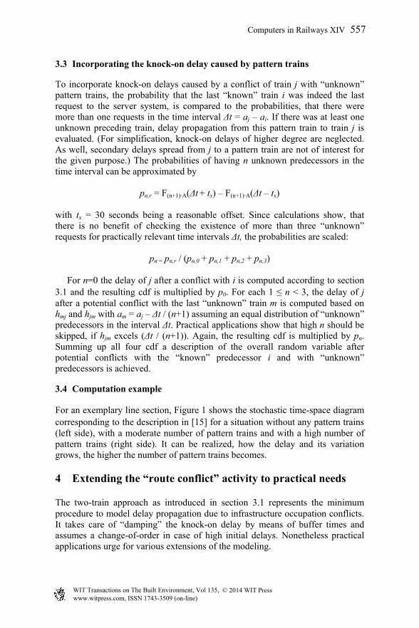
3.4 Computation example

For an exemplary line section, Figure 1 shows the stochastic time-space diagram corresponding to the description in [15] for a situation without any pattern trains (left side), with a moderate number of pattern trains and with a high number of pattern trains (right side). It can be realized, how the delay and its variation grows, the higher the number of pattern trains becomes.

4 Extending the “route conflict” activity to practical needs

The two-train approach as introduced in section 3.1 represents the minimum procedure to model delay propagation due to infrastructure occupation conflicts. It takes care of “damping” the knock-on delay by means of buffer times and assumes a change-of-order in case of high initial delays. Nonetheless practical applications urge for various extensions of the modeling.



Figure 2: Stochastic time-space diagram for different inter-arrival rates.

4.1 Approximating train kinematics by an offset

In general, minimum technical headway times describe the shortest time span for a jointly used section (e.g. line track or set of switches) which is required to avoid a hindrance of the second train by the first train. If the second train follows in a closer order, it would be subject to a restrictive signalling aspect and the overall capacity consumption would grow due to at least deceleration and acceleration phases. If there is an ATP- or ATC-system in situ, which is not capable of infill functionalities, the braking period may even last longer than required to ensure a semi-continuously supervised speed (Wendler introduces a powerful modeling approach by means of the “buffer-time equivalent” in [16].) The approach illustrated in section 3.1 incorporates the minimum headway time (indirectly via the related buffer time) to detect a conflict on the jointly used section. For this purpose, the minimum technical headway time is most appropriate. But since a train is solely shifted “behind” the minimum headway time in case of a conflict, if one stays at the formulas given in section 3.1, the resulting knock-on delay is too low, since neither deceleration nor acceleration phases are taken into account at all. In practical applications this imprecision proves to be relevant, since the overall amount of knock-on delays due to “route conflicts” considerably underruns the corresponding number in real operation, given a comparable delay level. To overcome this shortcoming, the knock-on delays should ideally be determined with respect to the deceleration and acceleration phases, including possible limitations caused by the ATP-/ATC-system. Accounting for this requirement is common in synchronous or asynchronous simulations based on a deterministic representation of delays, e.g. tools following the Monte-Carlo approach. In the given context, instead of incorporating the randomness by a series of simulation runs, the stochastic nature



of delays is directly considered by their representation and manipulation through cdf. Caring about constraints of mathematical independencies while formulating operations on random variables, a one-by-one translation of the deterministic solution to the stochastic environment is hardly feasible. As a workaround, an offset parameter ts is added to the resulting delay:

Vi,s = Vj,a + bij + hij + hji + ts for E3, Vi,s = Vi,a otherwise Vj,s = Vi – bij + ts for E2, Vj,s = Vj,a otherwise

For practical applications, the offset tS = 18 seconds has shaped up as convenient. An example on the impact is provided in section 4.4.

4.2 Attributing train paths with probabilities

To reduce the planning effort per freight-train path request and to achieve an “industrialisation” of the timetabling process, infrastructure managers more and more tend to offer standardised train paths to the market. These “catalogue” paths are setup between major nodes of the freight network and rely on minimum requirements on the traction power, train length and train mass. Like passenger-train paths, they are compiled in frequencies and thus allow a reoccurring hourly timetable pattern. If an individual train-path request adheres to the requirements of a catalogue path, it may easily be compiled by assembling a sequence of catalogue train path through the network. Beside their contribution to the reduction of planning efforts, catalogue freight train paths also provide benefits in operations, if there is a high share of similar freight services on a certain corridor, e. g. between two major hubs. Whenever a freight train is ready for departure, it may be “put” into the next suitable catalogue train path. Considering the compilation of catalogue train paths in advance of actual train-paths requests and their flexible usage by the next train of suitable characteristics, some train paths may remain unused in operation. For this case the stochastic modelling of delays is advantageous compared to a deterministic representation, because each train path may be attributed by its probability of running, which is taken into account, when there might be a knock-on delay caused to another train. For the “route conflict” activity introduced in section 3.1 this means two additional input parameters:

Probability of running of first train pi Probability of running of second train pj

In the computation of Vi,s and Vj,s the probability of events E2 respectively E3 is modified accordingly, reducing the amount of secondary delay. As well, the computation of indicators related to samples (e.g. punctuality at a specific station) can be extended to incorporate the probabilities of running per element within the sample to ensure an appropriate averaging.



4.3 Considering priorities with regard to the occupation ratio

To care about operational priorities, being for instance a function of the train type, the location and the time-of-day, the inequalities determining cases E1 to E4 may be extended by a dispatching offset dij with -hij ≤ dij ≤ hji as follows:

E1: Vi,a – Vj,a ≤ bij E2: bij < Vi,a – Vj,a ≤ bij + hij + dij E3: bij + hij + dij < Vi,a – Vj,a ≤ bij + hij + hji E4: bij + hij + hji < Vi,a – Vj,a

Depending on value of dij, the probability, whether the first or the second train is subject to a knock-on delay, is modified. By using extreme values either any secondary delay to the first or to the second train may be suppressed at all. For practical considerations, anyway, the concept of “partial priorities” is closer to reality, allowing delay propagation to the higher ranked train, too. For this purpose, a correction factor 0 ≤ fr ≤ 1 is introduced:

dij = fr · hji if the second train j is of higher priority (ri < rj) dij = 0 if both trains are of equal priority (ri = rj) dij = -fr · hij if the first train i is of higher priority (ri > rj)

Because in actual operation also higher ranked trains suffer from knock-on delays, the correction factor should account for this circumstance:

fr = |ri – rj| / (ri + rj)

With this formulation, the dispatching offset becomes the higher, the more different the priorities are. But, if both trains are of priority, the differentiation counts less. In general the introduction of operational priorities causes an increase of the overall delay level, since “suboptimal” conflict solutions are chosen and higher secondary delays have to be propagated. (For M/GI/1/∞ queuing systems, this relationship can nicely be proven by the formula of Pollaczek–Khinchine, because the dispatching offset dij increases the variance but not the expectation value of the service times, leading to higher waiting times respectively a longer waiting queue as shown in [17].) Applying the formulation just introduced and comparing the related simulation results to real-world data it becomes evident, that high-ranked trains suffer from too few secondary delays at major nodes of the network. This corresponds to the dispatcher’s philosophy of running trains by first-in-first-out philosophy, if there is a high infrastructure utilisation (which is in line to “optimal” amount of knock-on delays in case of fully equal ranks). To improve the significance of the achieved results, the dispatching offset dij thus needs to be linked to the individual infrastructure utilisation. For this purpose, the occupation ratio ρ is approximately derived at each affected server system by counting all requests trains in a time frame tF symmetrically surrounding the considered pair of trains i and j and by dividing the sum of the minimum headway times between all train pairs by the time period. If ρ exceeds a threshold ρmin, the correction term fr is attenuated in a linear manner:

fr = (|ri – rj| / (ri + rj)) · max (ρmax – ρ, 0) / (ρmax – ρmin)



For practical purposes, values of tF = 4 h, ρmin = 0.35 and ρmax = 0.65 have proven reasonable. Again, the impact on overall key figures is given below.

4.4 Computation examples

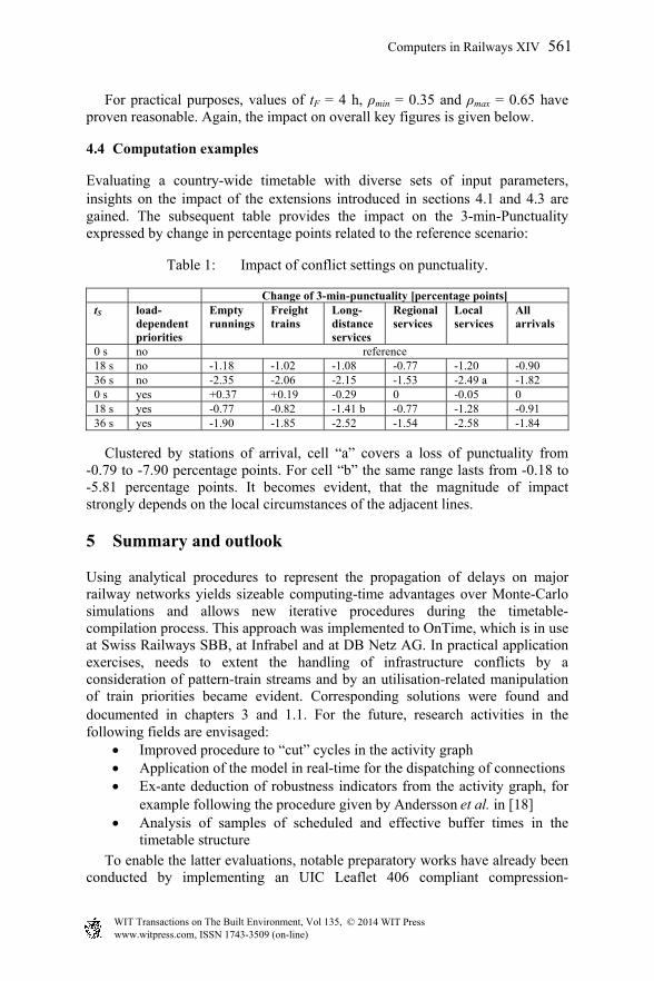
Evaluating a country-wide timetable with diverse sets of input parameters, insights on the impact of the extensions introduced in sections 4.1 and 4.3 are gained. The subsequent table provides the impact on the 3-min-Punctuality expressed by change in percentage points related to the reference scenario:

Table 1: Impact of conflict settings on punctuality.

Change of 3-min-punctuality [percentage points] tS load-

dependent priorities

Empty runnings

Freight trains

Long-distance services

Regional services

Local services

All arrivals

0 s no reference 18 s no -1.18 -1.02 -1.08 -0.77 -1.20 -0.90 36 s no -2.35 -2.06 -2.15 -1.53 -2.49 a -1.82 0 s yes +0.37 +0.19 -0.29 0 -0.05 0 18 s yes -0.77 -0.82 -1.41 b -0.77 -1.28 -0.91 36 s yes -1.90 -1.85 -2.52 -1.54 -2.58 -1.84

Clustered by stations of arrival, cell “a” covers a loss of punctuality from -0.79 to -7.90 percentage points. For cell “b” the same range lasts from -0.18 to -5.81 percentage points. It becomes evident, that the magnitude of impact strongly depends on the local circumstances of the adjacent lines.

5 Summary and outlook

Using analytical procedures to represent the propagation of delays on major railway networks yields sizeable computing-time advantages over Monte-Carlo simulations and allows new iterative procedures during the timetable-compilation process. This approach was implemented to OnTime, which is in use at Swiss Railways SBB, at Infrabel and at DB Netz AG. In practical application exercises, needs to extent the handling of infrastructure conflicts by a consideration of pattern-train streams and by an utilisation-related manipulation of train priorities became evident. Corresponding solutions were found and documented in chapters 3 and 1.1. For the future, research activities in the following fields are envisaged:

Improved procedure to “cut” cycles in the activity graph Application of the model in real-time for the dispatching of connections Ex-ante deduction of robustness indicators from the activity graph, for

example following the procedure given by Andersson et al. in [18] Analysis of samples of scheduled and effective buffer times in the

timetable structure

To enable the latter evaluations, notable preparatory works have already been conducted by implementing an UIC Leaflet 406 compliant compression-



approach, which allows the detection of “critical paths” through the timetable structure in the initial and the concatenated situation. Linking the compression of a timetable with the knowledge gathered from delay propagation may provide new insights into timetable dynamics in the future.

References

[1] Schwanhäußer, W. Die Bemessung der Pufferzeiten im Fahrplangefüge der Eisenbahn. Dissertation: RWTH Aachen, Germany, 1974.

[2] International Union of Railways (UIC). Capacity. Leaflet 406, Paris, France, 2004.

[3] Büker, T. Methods of assessing railway infrastructure capacity. At: 1st Workshop on Railway Systems Engineering, Karabük, Turkey, 2012.

[4] Vakhtel, S. Rechnerunterstützte analytische Ermittlung der Kapazität von Eisenbahnnetzen. Dissertation: RWTH Aachen, Germany, 2002.

[5] Janecek, D., Kuckelberg, A., Nießen, N. Kapazitätsermittlung von Eisenbahnknoten und Strecken. In: Eisenbahntechnische Rundschau (ETR), pp. 30-36, Germany, 2012.

[6] Kogel, B., Nießen, N., Büker, Th. Influence of the European Train Control System (ETCS) on the capacity of nodes. International Union of Railways (UIC), Paris, France, 2010. ISBN 978-2-7461-1801-0.

[7] Nießen, N. Schneider, W., Oetting, A. Moses/Wizug – Strategic modelling and simulation tool for rail freight transportation. In: Proceedings of the European Transport Conference, Session 11, Strasbourg, France, 2003.

[8] Weigand,W. Graphentheoretisches Verfahren zur Fahrplangestaltung in Transportnetzen unter Berücksichtigung von Pufferzeiten mittels interaktiver Rechentechnik. Dissertation: TU Braunschweig, Germany, 1981.

[9] Mühlhans, E. Berechnung der Verspätungsentwicklung bei Zugfahrten. In: Eisenbahntechnische Rundschau (ETR), pp. 465-469, Germany, 1990.

[10] Waas, K., Büker, Th. Effiziente Analyse von Fahrplankonzepten. In: Eisenbahntechnische Rundschau (ETR), pp. 738-743, Germany, 2008.

[11] Büker, Th. Ausgewählte Aspekte der Verspätungsfortpflanzung in Netzen. Dissertation: RWTH Aachen, Germany, 2010.

[12] Seybold, B., Büker, Th. Stochastic modelling of delay propagation in large networks. In: Journal of Rail Transport Planning & Management, Volume 2, Issues 1-2, 2012.

[13] Franke, B., Graffagnino, Th., Labermeier, H., Büker, Th. OnTime – Network-wide Analysis of Timetable Stability. In: Proceedings of the 5th International Seminar on Railway Operations Modelling and Analysis, Copenhagen, Denmark, 2013.

[14] Maricau, E., Scheerlinck, K., Tassenoy, S., Verboven, S., Büker, Th. Evaluating the robustness of a railway timetable: A practical approach. In: Proc. of the 5th International Seminar on Railway Operations Modelling and Analysis, Copenhagen, Denmark, 2013.



[15] Graffagnino, Th., Ensuring timetable stability with train traffic data. In: Computers in Railways, vol. XIII. WIT Press, New Forest, UK, 2012.

[16] Wendler, E. Influence of automatic train control components with an infill functionality on the performance behaviour of railway facilities. Research report commissioned by the International Union of Railways (UIC), Aachen, Germany, 2005.

[17] Hansen, I. A., Pachl, J. (Ed.) Railway Timetable & Traffic. Eurailpress, Hamburg, Germany, 2008.

[18] Andersson, E., Peterson, A., Törnquist Krasemann, J. Quantifying railway timetable robustness in critical points. In: Journal of Rail Transport Planning & Management, Volume 3, Issues 1-2, 2014.



Tuning delay-propagation models to meet practical … · Tuning delay-propagation models to meet...

Documents

Transcript of Tuning delay-propagation models to meet practical … · Tuning delay-propagation models to meet...