Tunable Isolated Attosecond X-ray Pulses withGigawatt Peak Power from a Free-Electron Laser

Joseph Duris∗1, Siqi Li∗1,2, Taran Driver1,4,5, Elio G. Champenois4,James P. MacArthur1,2, Alberto A. Lutman1, Zhen Zhang1, Philipp Rosenberger1,4,6,7,

Jeff W. Aldrich1, Ryan Coffee1,4, Giacomo Coslovich1, Franz-Josef Decker1,James M. Glownia1,4, Gregor Hartmann8, Wolfram Helml7,9,10, Andrei Kamalov2,4,

Jonas Knurr4, Jacek Krzywinski1, Ming-Fu Lin1, Megan Nantel1,2, Adi Natan4,Jordan O’Neal2,4, Niranjan Shivaram1, Peter Walter1, Anna Wang3,4,

James J. Welch1, Thomas J. A. Wolf4, Joseph Z. Xu11,Matthias F. Kling1,4,6,7, Philip H. Bucksbaum1,2,3,4, Alexander Zholents11,

Zhirong Huang1,3, James P. Cryan1,4,†, and Agostino Marinelli1,†1SLAC National Accelerator Laboratory, Menlo Park, CA, 94025, USA2Physics Department, Stanford University, Stanford, CA, 94305, USA

3Applied Physics Department, Stanford University, Stanford, CA, 94305, USA4Stanford PULSE Institute, SLAC National Accelerator Laboratory, Menlo Park, CA, 94025, USA

5The Blackett Laboratory, Imperial College, London, SW7 2AZ, UK6 Max Planck Institute of Quantum Optics, D-85748 Garching, Germany

7 Physics Department, Ludwig-Maximilians-Universitat Munich, 85748 Garching, Germany8Institut fur Physik und CINSaT, Universitat Kassel, Heinrich-Plett-Str. 40, 34132 Kassel, Germany

9 Zentrum fur Synchrotronstrahlung, Technische Universitat Dortmund,Maria-Goeppert-Mayer-Straße 2, 44227 Dortmund, Germany10 Physik-Department E11, Technische Universitat Munchen,

James Franck-Straße 1, 85748 Garching, Germany11Argonne National Laboratory, Lemont, IL, 60439, USA

∗These authors contributed equally to this work.†To whom correspondence should be addressed;

E-mail: marinelli@slac.stanford.edu, jcryan@slac.stanford.edu.

1

arX

iv:1

906.

1064

9v1

[ph

ysic

s.op

tics]

25

Jun

2019

The quantum mechanical motion of electrons in molecules and solids occurs

on the sub-femtosecond timescale. Consequently, the study of ultrafast elec-

tronic phenomena requires the generation of laser pulses shorter than 1 fs

and of sufficient intensity to interact with their target with high probability.

Probing these dynamics with atomic-site specificity requires the extension of

sub-femtosecond pulses to the soft X-ray spectral region. Here we report the

generation of isolated GW-scale soft X-ray attosecond pulses with an X-ray

free-electron laser. Our source has a pulse energy that is six orders of magni-

tude larger than any other source of isolated attosecond pulses in the soft X-ray

spectral region, with a peak power in the tens of gigawatts. This unique combi-

nation of high intensity, high photon energy and short pulse duration enables

the investigation of electron dynamics with X-ray non-linear spectroscopy and

single-particle imaging.

Introduction

The natural time scale of electron motion in molecular systems is determined by the binding

energy, Ip, typically between 8 and 12 eV. Quantum mechanics tells us that this relationship

is given by τ = h/Ip, where h is the reduced Planck constant. Therefore, the relevant time

scale for electron motion in molecular systems is on the order of a few hundred attoseconds

(1 as = 10−18 sec). Light pulses approaching this extreme timescale were first demonstrated

in 2001 (1). These early demonstrations employed a process called high harmonic genera-

tion (HHG), where a strong, infrared laser-field was used to coherently drive electrons in an

atomic or molecular gas, leading to high-order harmonic up-conversion of the driving laser

field (2–5). The extension of time-resolved spectroscopy into the attosecond domain has greatly

advanced our understanding of electron dynamics in atoms, molecules, and condensed matter

2

systems (6–8). This attosecond revolution has been almost exclusively driven by HHG based

sources (1,9–20), which have been recently extended to reach the soft X-ray wavelengths (above

280 eV (21)) and produce the shortest pulses ever recorded (22–25). Extending attosecond

pulse sources into the soft X-ray domain is particularly important because soft X-rays can ac-

cess core-level electrons whose absorption properties are sensitive probes of transient electronic

structure (26–28).

In parallel with the development of HHG, the last two decades have seen the rise of X-ray

free-electron lasers (XFELs), such as the Linac Coherent Light Source (LCLS), as the bright-

est sources of X-ray radiation (29–35). The working principle of an XFEL is based on the

interaction of a relativistic electron beam with an X-ray electric field in a long periodic array

of magnetic dipoles called an undulator (36–38). The radiation/electron interaction causes the

electron beam to re-organize itself in a sequence of microbunches shorter than the radiation

wavelength, which results in the coherent emission of X-ray radiation with a peak power many

orders of magnitude larger than the spontaneous level (37, 38). Compared to laser-based HHG

sources XFELs have a large extraction efficiency at X-ray wavelengths, typically of order 0.1%

or larger. With a typical electron beam peak power in the tens of terawatts range, the resulting

X-ray pulses have tens of gigawatts of peak power, several orders of magnitude larger than table-

top X-ray sources. Furthermore, the photon energy of FEL sources is easily tunable via small

configuration changes of the accelerator or the undulator. The shortest pulse achievable with

an XFEL is limited by the available amplification bandwidth, which is of similar magnitude to

their extraction efficiency ≤ 0.1% (36, 39). For example, the X-ray bandwidth of LCLS can

support pulses shorter than 1 fs for hard X-ray energies (40,41). However, the shortest possible

pulse duration increases to 1-2 fs for photon energies below 1 keV (42, 43), where the relevant

core-level absorption edges for light elements are found: carbon (280 eV), nitrogen (410 eV),

and oxygen (540 eV). In this letter, we report the generation and time-resolved measurement of

3

gigawatt-scale isolated attosecond soft X-ray pulses with an XFEL. The bandwidth limitation

of the XFEL was overcome by compressing the electron beam with a high-power infrared pulse,

a technique termed enhanced self-amplified spontaneous emission (ESASE) (44).

Figure 1 shows a schematic representation of our experimental setup named X-ray laser-

enhanced attosecond pulse generation (XLEAP). The energy distribution of the electron beam

is modulated by the resonant interaction with a high-power infrared pulse in a long-period

undulator (or wiggler) (44–46). This modulation is converted into one or more high-current

(∼ 10 kA) spikes by a magnetic chicane. The spikes are subsequently used in the undulator to

generate short X-ray pulses. This bunch compression method effectively broadens the XFEL

bandwidth and allows the generation of sub-fs pulses in the soft X-ray spectral region. In our

experiment, rather than using an external infrared laser as originally proposed by Zholents (44),

we employ the coherent infrared radiation emitted by the tail of the electron beam in the wiggler

to modulate the core of the electron beam (47,48). This method results in a phase-stable, quasi-

single-cycle modulation, and naturally produces a single high-current spike that can generate

an isolated attosecond pulse. Figures 1 (a-d) show the measured initial current profile and the

evolution of the phase-space of the core of the electron bunch during the three stages of ESASE

compression.

After separating the broad bandwidth X-ray pulses from the spent electron bunch, the X-ray

pulses are focused and temporally overlapped with a circularly polarized, 1.3 µm, infrared (IR)

laser field in a velocity map imaging (VMI) spectrometer (49). Photoelectrons ionized by the X-

ray pulse receive a “kick” proportional to the vector potential of the IR laser pulse at the time of

ionization (50). Through the interaction of the ionized electron with the dressing IR-laser field,

the temporal properties of the X-ray pulse are mapped onto the final momentum distribution

of the emitted photoelectrons (51–53). This technique was originally called the “attosecond

streak camera,” and is routinely used to measure the temporal profile of isolated attosecond

4

pulses from HHG sources (54). In contrast to measurements done with HHG sources, in this

work we are able to diagnose the single-shot pulse profile, rather than an average pulse shape.

Moreover, the shot-to-shot fluctuations (or jitter) in the relative arrival time between the X-ray

and optical field present at an FEL facility (55) makes single-shot measurements unavoidable.

This single shot measurement scheme was originally demonstrated at LCLS by Hartmann et al.,

who recovered the “time-energy structure” of SASE pulses produced by LCLS (43). We have

adapted this technique to measure the sub-femtosecond structure of the X-ray pulses produced

by XLEAP.

Results

Figure 2 (a) shows a single-shot measurement of the “streaked” photoelectron momentum dis-

tribution, which we use to reconstruct the full temporal profile of the X-ray pulse (53). The

raw data is filtered and down-sampled (Fig. 2 (b)) before being fed into the reconstruction al-

gorithm, which returns a pulse profile and corresponding photoelectron distribution (Fig. 2 (c)).

The robustness of this algorithm has been tested at length in Ref. (53), and is detailed in the

supplemental material. Figure 2 also shows representative temporal profiles retrieved from the

reconstruction at photon energies of 905 eV (panel d) and 570 eV (panel e). Figures 2 (f) and (g)

show the distribution of pulse widths (full width at half maximum of the intensity profile) re-

trieved from two large data sets at these photon energies. The data shows that the XLEAP setup

generates sub-femtosecond X-ray pulses, and we find a median duration of 284 as FWHM

(476 as) at 905 eV (570 eV). The pulse duration fluctuates on a shot-to-shot basis and half of

the single-shot measurements fall within a 106 as (166 as) window at 905 eV (570 eV). This

amount of fluctuations is consistent with numerical simulations of ESASE FEL operation (see

e.g. (56)). The estimated uncertainty on the single-shot pulse duration is between 10% and 30%

of the measured duration depending on the pulse energy and the amplitude of the streaking

5

laser field (a discussion on the experimental uncertainty of the measurement can be found in

the supplemental materials). The median pulse energy is 10 µJ at 905 eV and 25 µJ at 570 eV.

However, due to the intrinsic fluctuations of SASE FELs (39) we observe pulses well above the

mean value (up to 250 µJ for 570 eV, corresponding to a peak power in the hundreds of GW).

We note that for the 570 eV dataset we were only able to obtain converging reconstructions for

pulse energies higher than 130 µJ, corresponding to the top 8%. However, since the data at both

energies does not show a significant correlation between pulse energy and duration (Figure 2

panels (b) and (e)) we believe that the average pulse duration from this sample is representative

of the entire data set.

In a separate set of experiments we measured single-shot X-ray spectra with a grating spec-

trometer. Figure 3 shows a range of single-shot X-ray spectra recorded around 650 eV and

905 eV, and the distribution of the measured bandwidth (FWHM). The median FWHM band-

width is 7.5 eV and 5 eV for the 905 eV and 650 eV datasets respectively. The Fourier transform

limited (FTL) duration for a bandwidth of 7.5 eV (5 eV) is 240 as (365 as). The average pulse

duration recovered from our reconstruction at similar energies is within a factor of 2 of the

FTL value. This discrepancy is due to the beam-energy chirp introduced by longitudinal space-

charge forces within the high-current ESASE spike (57). This results in a residual chirp in the

emitted X-rays, which is reproduced in the reconstruction (see Supplemental Materials). Rip-

ples in the spectral intensity are visible in the 650 eV spectra and are due to interference with

satellite pulses. The pulse energies of these side pulses can be inferred from the single-shot

spectra and are typically less than 0.3% of the main pulse for 650 eV and negligible for 905 eV.

Considerations for Pump/Probe Spectroscopy

To put the results of our work in context, we detail the development of isolated attosecond pulse

sources in Figure 4, where we compare the measured pulse energy from existing attosecond

6

light sources with the requisite flux to saturate the ionization of 1s electrons in various atomic

systems. The saturation level serves as a coarse approximation to the energy required for a

pump/probe experiment, and sources within two orders of magnitude of saturation are likely

useful for pump/probe studies. The pulse energy produced by HHG sources decays very rapidly

with the photon energy and is several orders of magnitude below the threshold for non-linear

interaction in the soft X-ray range (E > 280 eV). Conversely our method can produce isolated

attosecond pulses with tens of µJ of pulse energy, increasing the available pulse energy at soft

X-ray wavelengths by six orders of magnitude, and reaching intensities sufficient for attosecond

pump/attosecond probe experiments. Note that Fig. 4 reports the pulse energy measured for the

experiments shown in Figs. 2 and 3, as well as other experiments using the XLEAP setup at

different photon energies. The highest observed median pulse energy is ∼ 50 µJ.

In addition to high single pulse photon flux, the application of this technique to attosecond

pump/attosecond probe experiments requires the generation of pairs of synchronized pulses.

Ideally these pulses could have different photon energies allowing for excitation at one atomic

site in a molecular system to be probed at another (58). To this end, ESASE can be easily

adapted to generate pairs of pulses of different colors using the split undulator method (59–61).

In this scheme the LCLS undulator is divided in two parts separated by a magnetic chicane, as

shown at the top of Fig. 5. The ESASE current spike is used to generate two X-ray pulses of

different energies in the two undulators. The magnetic chicane delays the electrons with respect

to the X-rays, thus introducing a controllable delay between the first and second X-ray pulses.

Figure 5 shows the results of such a double-pulse ESASE experiment at LCLS. Two pulses

with an average pulse energy of 6 µJ each and an energy separation of 15 eV were generated (see

Fig. 5 b). The timing jitter between the two pulses was not measured but numerical simulations

indicate that it is shorter than the individual pulse duration. We note that the energy separation

range in our experiment is limited by the tuning range of the LCLS undulator (roughly 3%

7

of the photon energy (59)), but this scheme could be used with variable gap undulators and

allow fully independent tuning of the two colors. This will be possible with the upcoming

LCLS-II upgrade, enabling continuous tuning between 250 eV and 1200 eV (62). The temporal

separation can be varied from a minimum of 2 fs up to a maximum of roughly 50 fs. Smaller

delays could be accessed with a gain-modulation scheme (61). Improved two-color operation

with higher peak power and delay control through overlap could be achieved with a modest

upgrade of the XLEAP setup (56).

Using the split-undulator scheme shown in Fig. 5 a, one can also generate two pulses of the

same photon energy and with mutual phase stability. Unlike the case of two different colors,

where the two pulses are seeded by noise at different frequencies and are uncorrelated, in this

case the beam microbunching that generates the first pulse is re-used to generate a second pulse

and the two are phase-locked. Figure 5c shows the measured spectra under these conditions.

The spectra exhibit stable and repeatable fringes, which implies that the phase between the two

pulses is stable to better than the X-ray wavelength. From the variation in the spectral fringes

we can infer a phase jitter of 0.77 rad, or 0.5 as between the pulses. In this case the delay can

be varied from 0 fs to roughly 5 fs. Beyond this value the delay chicane will destroy the X-ray

microbunching and hence the phase stability of the pulses.

Summary and conclusions

We have demonstrated tunable sub-femtosecond X-ray pulses with tens of gigawatts of peak

power using a free-electron laser. The pulses were generated by an electron bunch modulated

by interaction with a high-power infrared light pulse and compressed in a small magnetic chi-

cane. To diagnose the temporal structure of these pulses we used an attosecond streak camera

and measured a median pulse duration of 284 as (476 as) at 905 eV (570 eV). With an eye

towards pump/probe experiments, pairs of sub-fs pulses were demonstrated using a split undu-

8

lator technique, showing control of the delay and energy separation, but with a reduced peak

power compared to the single-pulse case.

These pulses have pulse energies six orders of magnitude higher than what can be achieved

with HHG based sources in the same wavelength range. The measured peak power is in the

tens to hundreds of gigawatts. Such a marked increase in pulse energy will enable a suite of

non-linear spectroscopy methods such as attosecond-pump/attosecond-probe experiments (63,

64) and four-wave mixing protocols (58). Moreover, the achieved photon flux is will enable

single-shot X-ray imaging at the attosecond timescale. Finally, the XLEAP setup is based on a

passive modulator and it is naturally scalable to the MHz-repetition rate envisioned for the next

generation of X-ray free-electron lasers (35, 62).

9

Wiggler

Undulator

Chicane

XTCAV

IR laser

E-beam

X-rays

(a) (b) (c) (d)

VMI

Fig. 1. Top: schematic representation of the experiment. The electron beam travels through

a long period (32 cm) wiggler and develops a single-cycle energy modulation. The energy mod-

ulation is turned into a density spike by a magnetic chicane and sent to the LCLS undulator to

generate sub-fs X-ray pulses. After the undulator the relativistic electrons are separated from the

X-rays and sent to a transverse cavity (labeled XTCAV) used for longitudinal measurements of

the beam. The X-rays are overlapped with a circularly polarized infrared laser (labeled IR laser)

and interact with a gas-jet to generate photoelectrons. The extracted photoelectrons are streaked

by the laser and detected with a velocity map imaging (VMI) spectrometer. The momentum dis-

tribution of the electrons is used to reconstruct the pulse profile in the time domain. Bottom:

measurements of the ESASE modulation process. (a) the measured current profile of the

electron bunch generated by the accelerator. The tail of the bunch has a high-current horn that

10

generates a high-power infrared pulse used for the ESASE compression. (b), (c) and (d) Show

the longitudinal phase-space of the core of the electron bunch in three different conditions: (b)

with no wiggler and no chicane we measure the electron distribution generated by the acceler-

ator; (c) after inserting the wiggler we observe a single-cycle energy modulation generated by

the interaction between electrons and radiation; (d) after turning on the chicane the modulation

is turned into a high current spike at t = -5 fs.

11

(a) (b) (c)

(d)

(e)

(f)

(g)

(h)

(i)

Fig. 2. Results of the angular streaking measurement. (a,b,c): measured and reconstructed

streaked photoelectron distribution from a single X-ray pulse. Our reconstruction algorithm

reads the photoelectron momentum distribution (a), downsamples the data (b) and fits it to

simulated streaked spectra calculated from a complete basis set (c). (d,e) Representative pulse

reconstruction at 905 eV (d) and 570 eV (e). The shaded blue lines represent the solutions found

from running the reconstruction algorithm initiated by different random seeds, and the red lines

represent the most probable solution (see Supplementary Material for details). The labeled

number is the averaged ∆τFWHM over the different solutions. (f,g): distribution of retrieved

X-ray pulse durations for 905 eV (f) and 570 eV (g). The red and blue vertical lines correspond

to the median of ∆τFWHM and ∆τRMS× 2√

2ln2 respectively. For 905 eV data, they are 284 as

12

and 355 as. For 570 eV data, they are 476 as and 505 as. (h,i): scatter plot of pulse energy as

a function of pulse duration for the reconstructed shots and a histogram of the pulse energy for

the entire data set for 905 eV (h) and 570 eV (i).

13

0

1

895 905 9150.0

2.5

Photon energy (eV)

Spect

ral in

tensi

ty (

uJ/eV

)

20 40 60Pulse energy (uJ)

0

100

200

5 10 15FWHM bandwidth (eV)

0

50

100

0.02.5

650 6550

10

Photon energy (eV)

Spect

ral in

tensi

ty (

uJ/eV

)a) b)

25 50 75Pulse energy (uJ)

0

20

40

5 10FWHM bandwidth (eV)

0

50

100

c) d)

e) f)

Fig. 3. (a,b) Spectra of the attosecond X-ray pulses measured with a grating spectrometer at

two different electron beam energies ((a): 3782.1 MeV; (b): 4500.3 MeV). The top figures show

average spectra at slightly different electron beam energies (in steps of 2.7 MeV for 650 eV and

3.0 MeV steps for 905 eV), while the remaining spectra show single-shot measurements at

the energy of the center curves shown in the top plots. (c,d): histogram of the distribution of

FWHM bandwidths. Panels (e,f) show a histogram of the distribution of pulse energies.

14

Fig. 4. Survey of published isolated attosecond pulse sources (1, 9–19, 22–24) extending into

the soft X-ray domain (red open circles), along with the results demonstrated in this work for

a number of different photon energies (red filled circles). The filled circle shows the average

pulse energy recorded during the experiment, the error bar extends from the central energy

and includes up to 90% of the recorded pulse energies. All previous results were obtained via

strong-field driven high harmonic generation with near-infrared and mid-infrared laser fields,

while our results are obtained using a free-electron laser (FEL) source. As a first-order estimate

of the propensity for nonlinear science (pump/probe spectroscopy, etc.) we show the pulse

energy required to saturate 1s ionization of carbon (dash-dot, black), nitrogen (dash-dot, blue),

oxygen (dash-dot, red), and helium (dash-dot, gray), assuming a 1 µm2 focal spot size, as a

15

function of X-ray photon energy. Sources within 2 orders of magnitude of the line are likely

sources for pump-probe studies. The table in the bottom right corner gives the published pulse

duration for the previous measurements. The shaded blue area shows the operational range

predicted for LCLS-II.

16

900 905 910Photon energy (eV)

4495

4500

4505Be

am e

nerg

y (M

eV)

900 905 910Photon energy (eV)

900 905 910Photon energy (eV)

925 930 935 940 945 950 955Frequency (eV)

0.0

0.2

0.4

0.6

0.8

1.0

1.2

Spec

tral

inte

nsity

(uJ/e

v)

mean1 shot

a)

b) c)

d) e) f)

undulator 1

wigglerchicane

undulator 2

chicane

e-beam

Fig. 5. (a): Schematic representation of the double pulse generation experiment. The electron

beam is modulated and compressed in the XLEAP beamline and sent to the LCLS undulator.

The undulator is divided in two parts separated by a magnetic chicane. Each half of the undula-

tor is used to generate an X-ray pulse with different pulse energies, and the chicane introduces a

variable delay between the pulses. (b): Single shot and average two-color spectra measured with

a grating spectrometer. (c): Single-shot measurements of the spectrum of the pulse pair with

1 fs delay. The repeatable spectral fringe demonstrate phase stability between the pulses. (d),

(e), (f): Averaged phase-stable double shot spectra as a function of photon energy and electron

beam energy for a nominal chicane delay of 0 fs (single pulse)(d), 0.5 fs (e) and 3 fs (f).

17

Supplementary materials

Materials and Methods

Supplementary Text

Figs. S1 to S12

References (65-78)

References

1. M. Hentschel, et al., Nature 414, 509 (2001).

2. X. F. Li, A. LHuillier, M. Ferray, L. A. Lompr, G. Mainfray, Physical Review A 39, 5751

(1989).

3. J. L. Krause, K. J. Schafer, K. C. Kulander, Physical Review Letters 68, 3535 (1992).

4. P. B. Corkum, Physical Review Letters 71, 1994 (1993).

5. M. Chini, K. Zhao, Z. Chang, Nature Photonics 8, 178 (2014).

6. P. B. Corkum, F. Krausz, Nature Physics 3, 381 (2007).

7. Z. Chang, P. Corkum, JOSA B 27, B9 (2010).

8. M. F. Ciappina, et al., Reports on Progress in Physics 80, 054401 (2017).

9. T. Sekikawa, A. Kosuge, T. Kanai, S. Watanabe, Nature 432, 605 (2004).

10. G. Sansone, et al., Science 314, 443 (2006).

11. I. J. Sola, et al., Nature Physics 2, 319 (2006).

12. E. Goulielmakis, et al., Science 320, 1614 (2008).

18

13. H. Mashiko, et al., Physical Review Letters 100, 103906 (2008).

14. X. Feng, et al., Physical Review Letters 103, 183901 (2009).

15. F. Ferrari, et al., Nature Photonics 4, 875 (2010).

16. E. J. Takahashi, P. Lan, O. D. Mcke, Y. Nabekawa, K. Midorikawa, Nature Communications

4, 2691 (2013).

17. M. Ossiander, et al., Nature Physics 13, 280 (2017).

18. T. R. Barillot, et al., Chemical Physics Letters 683, 38 (2017).

19. B. Bergues, et al., Optica 5, 237 (2018).

20. O. Jahn, et al., Optica 6, 280 (2019).

21. D. Attwood, A. Sakdinawat, X-rays and extreme ultraviolet radiation: principles and ap-

plications (Cambridge university press, 2017).

22. S. M. Teichmann, F. Silva, S. L. Cousin, M. Hemmer, J. Biegert, Nature Communications

7, 11493 (2016).

23. T. Gaumnitz, et al., Optics Express 25, 27506 (2017).

24. J. Li, et al., Nature Communications 8, 186 (2017).

25. A. S. Johnson, et al., Science Advances 4, eaar3761 (2018).

26. T. J. A. Wolf, et al., Nature Communications 8, 29 (2017).

27. S. P. Neville, M. Chergui, A. Stolow, M. S. Schuurman, Physical Review Letters 120,

243001 (2018).

19

28. A. R. Attar, et al., Science 356, 54 (2017).

29. W. Ackermann, et al., Nature photonics 1, 336 (2007).

30. P. Emma, et al., Nat Photon 4, 641 (2010).

31. E. Allaria, et al., Nat Photon 6, 699 (2012).

32. E. Allaria, et al., Nat Photon 7, 913 (2013).

33. T. Ishikawa, H. Aoyagi, T. Asaka, al., Nat Photon 6, 540 (2012).

34. H.-S. Kang, et al., Nature Photonics 11, 708 (2017).

35. M. Altarelli, Nuclear Instruments and Methods in Physics Research Section B: Beam In-

teractions with Materials and Atoms 269, 2845 (2011).

36. R. Bonifacio, C. Pellegrini, L. Narducci, Optics Communications 50, 373 (1984).

37. C. Pellegrini, A. Marinelli, S. Reiche, Rev. Mod. Phys. 88, 015006 (2016).

38. Z. Huang, K.-J. Kim, Phys. Rev. ST Accel. Beams 10, 034801 (2007).

39. R. Bonifacio, L. De Salvo, P. Pierini, N. Piovella, C. Pellegrini, Phys. Rev. Lett. 73, 70

(1994).

40. S. Huang, et al., Physical review letters 119, 154801 (2017).

41. A. Marinelli, et al., Applied Physics Letters 111, 151101 (2017).

42. C. Behrens, et al., Nature Communications 5, 3762 (2014).

43. N. Hartmann, et al., Nature Photonics 12, 215 (2018).

20

44. A. A. Zholents, Physical Review Special Topics - Accelerators and Beams 8, 040701

(2005).

45. A. A. Zholents, W. M. Fawley, Phys. Rev. Lett. 92, 224801 (2004).

46. E. Hemsing, G. Stupakov, D. Xiang, A. Zholents, Reviews of Modern Physics 86, 897

(2014).

47. J. MacArthur, et al., Submitted to Phys. Rev. Lett. (2019).

48. J. MacArthur, J. Duris, Z. Huang, A. Marinelli, Z. Zhang, Proc. 9th International Particle

Accelerator Conference (IPAC’18), Vancouver, BC, Canada, April 29-May 4, 2018, no. 9

in International Particle Accelerator Conference (JACoW Publishing, Geneva, Switzerland,

2018), pp. 4492–4495. Https://doi.org/10.18429/JACoW-IPAC2018-THPMK083.

49. S. Li, et al., AIP Advances 8, 115308 (2018).

50. R. Kienberger, et al., Nature 427, 817 (2004).

51. A. K. Kazansky, A. V. Bozhevolnov, I. P. Sazhina, N. M. Kabachnik, Physical Review A

93, 013407 (2016).

52. A. K. Kazansky, I. P. Sazhina, V. L. Nosik, N. M. Kabachnik, Journal of Physics B: Atomic,

Molecular and Optical Physics 50, 105601 (2017).

53. S. Li, et al., Optics Express 26, 4531 (2018).

54. J. Itatani, et al., Physical Review Letters 88, 173903 (2002).

55. J. M. Glownia, et al., Optics Express 18, 17620 (2010).

56. Z. Zhang, J. Duris, J. P. MacArthur, Z. Huang, A. Marinelli, Phys. Rev. Accel. Beams 22,

050701 (2019).

21

57. Y. Ding, Z. Huang, D. Ratner, P. Bucksbaum, H. Merdji, Phys. Rev. ST Accel. Beams 12,

060703 (2009).

58. S. Mukamel, D. Healion, Y. Zhang, J. D. Biggs, Annual Review of Physical Chemistry 64,

101 (2013).

59. A. A. Lutman, et al., Phys. Rev. Lett. 110, 134801 (2013).

60. T. Hara, et al., Nat Commun 4 (2013).

61. A. Marinelli, et al., Physical Review Letters 111, 134801 (2013).

62. R. Schoenlein, New Science Opportunities Enabled by LCLS-II X-ray Lasers (2015).

63. S. R. Leone, et al., Nature Photonics 8, 162 (2014).

64. I. V. Schweigert, S. Mukamel, Physical Review A 76, 012504 (2007).

Acknowledgements

The authors would like to acknowledge Tais Gorkhover, Christoph Bostedt, Jon Marangos,

Claudio Pellegrini, Adrian Cavalieri, Nora Berrah, Linda Young, Lou DiMauro, Heinz-Dieter

Nuhn, Gabriel Marcus, and Tim Maxwell for useful discussions and suggestions. We would also

like to acknowledge Michael Merritt, Oliver Schmidt, Nikita Strelnikov, Isaac Vasserman for

their assistance in designing, constructing and installing the XLEAP wiggler. We also acknowl-

edge the SLAC Accelerator Operations group, and the Mechanical and Electrical engineering

divisions of the SLAC Accelerator Directorate, especially Gene Kraft, Manny Carrasco, Anto-

nio Cedillos, Kristi Luchini and Jeremy Mock for their invaluable support.

This work was supported by U.S. Department of Energy Contracts No. DE-AC02-76SF00515,

DOE-BES Accelerator and detector research program Field Work Proposal 100317, DOE-BES,

22

Chemical Sciences, Geosciences, and Biosciences Division, and Department of Energy, Labo-

ratory Directed Research and Development program at SLAC National Accelerator Laboratory,

under contract DE-AC02-76SF00515. WH acknowledges financial support by the BACATEC

programme. P.R. and M.F.K. acknowledge additional support by the DFG via KL-1439/10, and

the Max Planck Society. G. H. acknowledges the Deutsche Forschungsgemeinschaft (DFG,

German Research Foundation) Projektnummer 328961117 SFB 1319 ELCH.

23

Supplemental Material for Tunable IsolatedAttosecond X-ray Pulses with Gigawatt Peak Power

from a Free-Electron Laser

Joseph Duris∗1, Siqi Li∗1,2, Taran Driver1,4,5, Elio G. Champenois4,James P. MacArthur1,2, Alberto A. Lutman1, Zhen Zhang1, Philipp Rosenberger1,4,6,7,

Jeff W. Aldrich1, Ryan Coffee1,4, Giacomo Coslovich1, Franz-Josef Decker1,James M. Glownia1,4, Gregor Hartmann8, Wolfram Helml7,9,10, Andrei Kamalov2,4,

Jonas Knurr4, Jacek Krzywinski1, Ming-Fu Lin1, Megan Nantel1,2, Adi Natan4,Jordan O’Neal2,4, Niranjan Shivaram1, Peter Walter1, Anna Wang3,4,

James J. Welch1, Thomas J. A. Wolf4, Joseph Z. Xu11,Matthias F. Kling1,4,6,7, Philip H. Bucksbaum1,2,3,4, Alexander Zholents11,

Zhirong Huang1,3, James P. Cryan1,4,†, and Agostino Marinelli1,†1SLAC National Accelerator Laboratory, Menlo Park, CA, 94025, USA2Physics Department, Stanford University, Stanford, CA, 94305, USA

3Applied Physics Department, Stanford University, Stanford, CA, 94305, USA4Stanford PULSE Institute, SLAC National Accelerator Laboratory, Menlo Park, CA, 94025, USA

5The Blackett Laboratory, Imperial College, London, SW7 2AZ, UK6 Max Planck Institute of Quantum Optics, D-85748 Garching, Germany

7 Physics Department, Ludwig-Maximilians-Universitat Munich, 85748 Garching, Germany8Institut fur Physik und CINSaT, Universitat Kassel, Heinrich-Plett-Str. 40, 34132 Kassel, Germany

9 Zentrum fur Synchrotronstrahlung, Technische Universitat Dortmund,Maria-Goeppert-Mayer-Straße 2, 44227 Dortmund, Germany10 Physik-Department E11, Technische Universitat Munchen,

James Franck-Straße 1, 85748 Garching, Germany11Argonne National Laboratory, Lemont, IL, 60439, USA

∗These authors contributed equally to this work.

1

arX

iv:1

906.

1064

9v1

[ph

ysic

s.op

tics]

25

Jun

2019

Contents

1 Materials and Methods 2

1.1 Beam Dynamics and FEL Configuration . . . . . . . . . . . . . . . . . . . . . 2

1.1.1 Longitudinal Phase-Space Measurements . . . . . . . . . . . . . . . . 6

1.2 Angular Streaking Setup . . . . . . . . . . . . . . . . . . . . . . . . . . . . . 8

1.2.1 Laser X-ray Timing Stability . . . . . . . . . . . . . . . . . . . . . . . 9

1.3 Photoelectron Data Analysis Procedure . . . . . . . . . . . . . . . . . . . . . 10

1.4 Reconstruction Algorithm . . . . . . . . . . . . . . . . . . . . . . . . . . . . 12

1.4.1 Quantification of the single-shot experimental uncertainty . . . . . . . 17

2 Supplemental Text 18

2.1 Two-Color Pulse Properties . . . . . . . . . . . . . . . . . . . . . . . . . . . . 18

2.2 Machine Parameter Correlations . . . . . . . . . . . . . . . . . . . . . . . . . 19

1 Materials and Methods

1.1 Beam Dynamics and FEL Configuration

The x-ray free-electron laser (XFEL) at the Linac Coherent Light Source (LCLS) is composed

of a high-brightness linear accelerator (linac) and a magnetic undulator. The XLEAP beamline

is composed of a long-period wiggler and a magnetic chicane prior to the undulator section. The

accelerator and undulator/wiggler parameters used in this experiment are summarized in Tab. 1.

2

Accelerator and Undulator ParametersBeam Energy 3-5 GeVRepetition rate 120 HzNormalized Emittance 0.4 µmPeak Current Before ESASE Compression 2.5 - 3.5 kAPeak Current After ESASE Compression (estimated) ∼ 10 kAXLEAP Wiggler Period λw 32 cmXLEAP Wiggler Parameter Kw 0 - 52XLEAP Chicane Longitunal Dispersion R56 0 - 0.9 mmUndulator Period λu 3 cmUndulator Parameter Ku 3.45 - 3.51

The radiation wavelength generated by the XFEL is given by the well known resonant for-

mula (65):

λr = λu1 + K2

u

2

2γ2(1)

where γ is the Lorentz factor of the electron beam (between 6000 and 10000 for this experi-

ment). Similarly, the radiation wavelength generated in the wiggler (and therefore the electron

beam modulation wavelength) is given by

λIR = λw1 + K2

w

2

2γ2. (2)

The XLEAP beamline was designed to provide a modulation wavelength in the range be-

tween 2 and 4 µm for a beam energy between 3 and 5 GeV. At these beam energies the LCLS

undulator produces photons with an energy between ∼400 and ∼1200 eV. The amplitude of

the observed energy modulation is typically in the few MeV range and can be fully compressed

with the available dispersion of the XLEAP chicane. The self-modulation process has been

described in detail in (66).

The high-current spike generated by the XLEAP modulator generates strong longitudinal

space-charge forces which result in a strong time-energy correlation on the electrons within the

spike (67). The longitudinal space-charge force for a highly relativistic beam in an undulator is

3

proportional to the derivative of the longitudinal current profile:

Ez(s) = −Z0I′(s)(1 + K2

2)

4πγ2

2 log

γσz

rb√

1 + K2

2

(3)

where I(s) is the beam current as a function of the longitudinal coordinate s, σz is the length of

the current spike, and rb is the beam radius. For a Gaussian-like spike such as the one generated

by an ESASE modulator, the correlated energy spread (or chirp) is predominantly linear but has

a non-vanishing nonlinear component. The observed final energy distribution has a full width

in the range between 30 and 40 MeV, over a spike duration of order 1 fs. The bandwidth of this

chirp is much larger than the acceptance of the FEL.

To preserve the FEL gain with such a large energy spread the undulator parameter K has to

be varied (tapered) along the undulator length so that the resonant condition is maintained as

the photons slip ahead of the electrons and interact with electrons of a different energy (67–69).

This chirp-taper matching condition can be expressed as:

K

1 +K2

dKu

dzλw =

dγ

dsλr, (4)

where z is the position along the undulator beamline. The chirp-taper matching condition can

only be verified for a specific value of the linear chirp dγ/ds, meaning that if we optimize

the undulator to lase in the ESASE spike, the rest of the bunch will be mismatched in energy,

therefore suppressing the background radiation outside of the main pulse. Furthermore it can

be shown that the cubic chirp introduced by space-charge contributes to shortening the pulse

duration when the taper is optimized to compensate the linear chirp (69).

To take advantage of these two effects we maximized the chirp introduced by space-charge

by only allowing the electron beam to lase in the last few sections of our undulator beamline,

and suppressing the FEL gain in the first part of the undulator by introducing a large transverse

oscillation in the electron beam trajectory. Figure S1 shows an example of a typical undulator

4

0 20 40 60 80 100 120z (m)

3.44

3.46

3.48

3.5

Und

ulat

or K

0 20 40 60 80 100 120z (m)

-0.4

-0.2

0

0.2

Posi

tion

(mm

)

x-orbity-orbit

Lasing Suppressed Lasing On

Figure S1: Top: typical undulator configuration for an ESASE experiment. The FEL gainis suppressed in the first 24 undulators by a large oscillation in the vertical trajectory of theelectron beam. Bottom: measured vertical and horizontal trajectory through the undulators.

configuration for an ESASE experiment. The last 7 undulators are used for lasing, while the

remaining 24 are used to maximize the energy chirp introduced by space-charge. The electron

beam trajectory is also plotted, showing a large vertical oscillation in the first 24 undulators to

suppress the FEL gain.

The space-charge induced energy-spread can be seen in Fig. 1-d of the main text, which

shows the measured time-energy distribution of the full electron bunch. The ESASE current

spike is seen as a large vertical stripe, i.e. a short region of the bunch with a large energy

spread. The resolution of our diagnostic is not enough to resolve the sub-fs structure of the

phase-space, and therefore the chirp of the ESASE spike itself appears as a vertical stripe with

no apparent time-energy correlation.

5

75 50 25 0 25 50 75Time (fs)

3380

3400

3420

3440

3460

3480

Ener

gy (M

eV)

30 20 10 0 10 20 30Time (fs)

3360

3380

3400

3420

3440

3460

3480

Ener

gy (M

eV)

30 20 10 0 10 20 30Time (fs)

3360

3380

3400

3420

3440

3460

3480

Ener

gy (M

eV)

a) b) c)

wiggler in wiggler inchicane on

7550250255075Time (fs)

3380

3400

3420

3440

3460

3480

Energy (MeV)

3020100102030Time (fs)

3360

3380

3400

3420

3440

3460

3480

Energy (MeV)

3020100102030Time (fs)

3360

3380

3400

3420

3440

3460

3480

Energy (MeV)

a)b)c)

wiggler inwiggler inchicane on

7550250255075Time (fs)

3380

3400

3420

3440

3460

3480

Energy (MeV)

3020100102030Time (fs)

3360

3380

3400

3420

3440

3460

3480

Energy (MeV)

3020100102030Time (fs)

3360

3380

3400

3420

3440

3460

3480

Energy (MeV)

a)b)c)

wiggler inwiggler inchicane on

7550250255075Time (fs)

3380

3400

3420

3440

3460

3480

Energy (MeV)

3020100102030Time (fs)

3360

3380

3400

3420

3440

3460

3480

Energy (MeV)

3020100102030Time (fs)

3360

3380

3400

3420

3440

3460

3480

Energy (MeV)

a)b)c)

wiggler inwiggler inchicane on

Wiggler In Wiggler In Chicane On

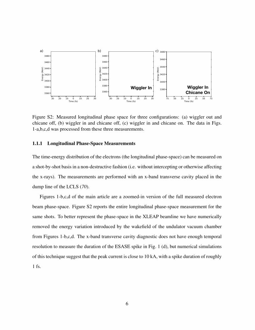
Figure S2: Measured longitudinal phase space for three configurations: (a) wiggler out andchicane off, (b) wiggler in and chicane off, (c) wiggler in and chicane on. The data in Figs.1-a,b,c,d was processed from these three measurements.

1.1.1 Longitudinal Phase-Space Measurements

The time-energy distribution of the electrons (the longitudinal phase-space) can be measured on

a shot-by-shot basis in a non-destructive fashion (i.e. without intercepting or otherwise affecting

the x-rays). The measurements are performed with an x-band transverse cavity placed in the

dump line of the LCLS (70).

Figures 1-b,c,d of the main article are a zoomed-in version of the full measured electron

beam phase-space. Figure S2 reports the entire longitudinal phase-space measurement for the

same shots. To better represent the phase-space in the XLEAP beamline we have numerically

removed the energy variation introduced by the wakefield of the undulator vacuum chamber

from Figures 1-b,c,d. The x-band transverse cavity diagnostic does not have enough temporal

resolution to measure the duration of the ESASE spike in Fig. 1 (d), but numerical simulations

of this technique suggest that the peak current is close to 10 kA, with a spike duration of roughly

1 fs.

6

x X-ray polarized in x

CCD camera

holey mirror

vacuum chamber

cVMI

interaction region gas jet into the page

MCP

( )

dichroic mirror IR pulse IR wave-plate x

z

x

y

focusing lens

Figure S3: Experimental geometry of the co-axial velocity map imaging (c-VMI) apparatusused in the angular streaking setup. Linearly polarized x-rays pass through a 2 mm hole in asilver coated mirror before coming to a focus in the interaction region of the cVMI spectrom-eter. Photoelectrons are extracted by the electrostatic field of the spectrometer, in the directionopposite of the x-ray propagation. The phosphor screen of the charged particle detector is im-aged via the holey silver mirror, through a dichroic mirror used to introduce an IR laser pulse.The polarization of the IR pulse is controlled via a quarter wave-plate upstream of the dichroicmirror. The target gas is introduced via a skimmed molecular beam oriented in the y-direction.

7

1.2 Angular Streaking Setup

Our experiment was performed at the Atomic, Molecular, and Optical physics (AMO) beam-

line of the Linac Coherent Light Source (LCLS). The streaking laser pulse is derived from a

120 Hz titanium-doped sapphire laser system synchronized to the accelerator. Ten mJ, 800 nm

laser pulses are compressed to ∼ 40 fs, and the compressed pulse is used to pump an optical

parametric amplifier (TOPAS-HE, Light Conversion) which produces 500 µJ pulses at a wave-

length of 1300 nm. The 1300 nm pulse is spectrally filtered to remove any residual pump light

or any other colors made by the OPA. A quarter waveplate (Thorlabs AQWP05M-1600) is used

to produce circularly polarized laser pulses, which are then focused with a f = 750 mm CaF2

lens. As shown in Fig. S3, a dichroic mirror (R1300/T400-550) is used to steer the beam into a

vacuum chamber. The streaking laser field is combined with the FEL beam using a silver mirror

with a 2 mm drilled hole, and both pulses come to a common focus in the interaction reagion of

a co-axial velocity map imaging (c-VMI) apparatus (71). To generate a reference measurement,

the streaking laser was intentionally mistimed every 11 XFEL shots. The c-VMI used here is

designed for angular streaking applications, and the device is described in Ref. (71). The x-ray

focal spot is approximately ∼ 55 µm diameter (FWHM), while the streaking laser focus is sub-

stantially larger,∼ 110 µm diameter. A target gas is introduced via a molecular beam source.

For the two x-ray photon energies considered in the main text, we use neon as the target for

905 eV pulses and CO2 as the target for 570 eV pulses.

Photoelectrons produced by two-color ionization are extracted opposite to the laser propaga-

tion direction, as shown in Fig. S3. This geometry is used to minimize any signal from scattered

x-ray photons. Extracted electrons are detected with a microchannel plate detector coupled to a

P43 phosphor screen. The phosphor screen is imaged onto a high-speed CCD camera (Opal1k)

via the 2 mm holey mirror which couples the streaking laser into the chamber, and through the

dichroic mirror. The CCD camera records images of the phosphor screen at the repetition rate

8

Figure S4: Two-dimensional projection of the photoelectron momentum distribution generatedby the IR laser in CO2 gas jet. This data was integrated over 4 × 104 laser shots. The ratio ofionization along the major axis to the minor axis is 10:1, which corresponds to an ellipticity ofε ∼ 0.95.

of the accelerator, 120 Hz.

We can diagnose the streaking laser polarization using the photoelectron momentum distri-

bution from strong-field ionization of a xenon target. Figure S4 shows the two-dimensional pro-

jection of the photoelectron momentum distribution produced by ionization with the 1300 nm

laser. We can estimate the ellipticity of the streaking laser by comparing the ionization probabil-

ity along the major and minor axes of the laser polarization. Using ADK theory the differential

ionization rate shown in Figure S4 gives a rough estimate of the ellipticity of ε ∼ 0.95 for the

IR streaking laser.

1.2.1 Laser X-ray Timing Stability

Synchronization between the attosecond X-ray pulses and the streaking pulses is a persistent

challenge in our measurement. Measurements at the LCLS use conventional feedback tech-

niques to stabilize the optical laser pulse arrival time relative to a radio frequency (RF) reference

from the accelerator (72). The primary sources for the temporal jitter include thermal effects,

RF noise, and energy jitter in the electron bunch. The electron bunches accumulate additional

9

Figure S5: Distributions of the extracted streak magnitudes as a function of the bunch arrivaltime with (a) a mistimed streaking laser and (b) a co-timed streaking laser. The black curvesshow the average streaking magnitude. (c) Comparison of the streaking magnitude’s depen-dence on the bunch arrival time (black, left axis) and the distribution of bunch arrival times(red, right axis).

temporal jitter as they propagate along the acceleration and bunch compression chain. This en-

ergy jitter is directly transformed into a timing jitter in the magnetic chicane bunch compressors.

Using a transverse cavity just before the electron beam dump, we can measure the shot-to-shot

variation between the arrival time of the electron bunch and the RF reference. Figure S5 shows

the distribution of measured streaking magnitudes for each shot as a function of the bunch ar-

rival time (BAT). The peak of the streaking magnitude distribution is offset from the nominal

0 fs BAT by ∼60 fs due to a slight mistiming of the streaking laser. We observe streaking over

a ∼300 fs range of BATs. This range is affected by both the streaking laser pulse width and the

streaking laser timing jitter with respect to the RF reference.

1.3 Photoelectron Data Analysis Procedure

We select shots to analyze based on the single shot pulse energy, streaking angle, and streak-

ing amplitude. Pulse energy is measured in the standard non-intrusive method employed at

the LCLS, by recording the flourescence induced by the x-ray pulse in a small (0.02–1.2 Torr)

10

Figure S6: Measurement of photoelectrons by the c-VMI. (a) raw, unprocessed image of asingle-shot measurement of neon 1s photoelectrons ionized by a 905 eV ESASE pulse withoutthe streaking laser. (b) raw single-shot image of neon 1s photoelectrons measured at the samephoton energy in the presence of the circularly polarized streaking field, shifting the momentumdistribution of the photoelectrons and encoding the properties of the ESASE pulse. This shiftis made clear in panel (c), showing the difference in measured electron counts between the shotshown in panel (b) and a background image constructed from multiple measurements of theunstreaked photoelectron distribution.

pressure of nitrogen (73). Filtering on pulse energy ensures the analyzed shots have a high

number of electron counts, which provides better quality reconstructions. A number of comple-

mentary techniques provide real-time information on the shot-to-shot amplitude and direction

of the momentum shift from the streaking laser. To process the shots, we identify these two

streaking coordinates using a genetic optimization algorithm which approximates the centroid

of the shifted electron distribution, by maximizing the electron density falling in an open ring

shape as the shape is shifted across the c-VMI image (74). For the reconstruction, we select

shots that are streaked perpendicular to the x-ray polarization, within an angular acceptance of

∼ 40◦/∼ 65◦ for the 905 eV and 570 eV shots respectively. This is a result of the 6 mm hole

in the center of the detector (71) and the angular distribution of the photoelectrons produced

by the two-color ionization, which approaches a cos2 θ dipole distribution (see Fig. S6). Shots

streaked parallel to the x-ray polarization suffer from a greater distortion of signal because the

corresponding momentum shift is along the axis of the highest electron density, maximizing the

11

electron signal lost by virtue of ‘falling’ into the hole. The converse is true for shots streaked

perpendicular to the x-ray polarization. We have verified that the measured pulse duration is

not correlated with either pulse energy or streak angle.

Single-shot CCD images, representative examples of which are shown in Fig. S6, are ana-

lyzed in the following way. First, a quadrant dependent gain correction is applied to the image

to account for the variation in camera gain between the four quadrants of the detector, and we

shift the center of the image to match the symmetry center found from unstreaked images. Then

we apply a median filter with a neighborhood size of 19 pixels, and the resulting image is con-

volved with a Gaussian filter (σ =25 pixels). The filtered image is then downsized from the

initial 1024×1024 image to 32×32 pixels. A background image, primarily consisting of low

energy electrons at the center of the detector, was obtained from the unstreaked images. This

background is subtracted from the downsized image. Incomplete suppression of this electron

background for the 905 eV pulse measurements results in an small artifact in the time domain

pulse reconstruction (a < 10% feature appearing exactly half the streaking laser period away

from the measured pulse). This is removed post-processing. Subtraction of this background

from a single shot image inevitably leads to small negative values in some pixels. Following

background subtraction, we threshold the image by the absolute value of the most negative pixel

intensity of the single shot image.

1.4 Reconstruction Algorithm

The pulse reconstruction algorithm is described in our previous publication (75). The algorithm

is based on the forward propagation of a basis set. We assume that the photoionized electron

wavepacket (EWP) can be described by a set of basis functions, αn:

ψ(t) = ~EX(t) · ~d(~p− ~A(t)) =∑

n

cn αn(t). (5)

12

The EWP, ψ(t), is given by the product of the x-ray electric field, ~EX(t), and the dipole mo-

ment, ~d(~p), describing the x-ray photoionization process, and ~A(t) is the vector potential of the

streaking laser field. The two-color photoelectron momentum distribution for an arbitrary x-ray

pulse can be calculated in the strong field approximation (SFA) (76):

b(~p) =∫ ∞

−∞~EX(t) · ~d(~p− ~A(t)) e−iΦ(t) dt, (6)

Φ(t) =∫ ∞

tdt′

(~p− ~A(t′))2

2+ Ip

, (7)

b(~p) is the probability amplitude for observing an electron with momentum ~p, and Ip is the

binding energy of the ionized electron. We assume the dipole moment is described by a hydro-

genic model: ~d(~p) = ~p/(|~p|2 − 2Ip)3. Each basis function, αn(t), will produce a probability

amplitude, an(~p) for observing an electron with momentum ~p according to:

an(~p) =∫ ∞

−∞~αn(t) · ~d(~p− ~A(t)) e−iΦ(t) dt. (8)

The total probability amplitude, b(~p), for the EWP in Eq. 5 is given by,

b(~p) =∑

n

cnan(~p). (9)

The measured photoelectron momentum distribution is given by the

B(~P ) =∫dpz |b(~p)|2 =

∑

nm

c∗mcn

∫dpza

∗m(~p)an(~p), (10)

where ~P is the two-dimensional vector describing the projected momentum. While Eqs. 6–13

are general for any choice of basis function, in this work we choose to construct the basis func-

tions αn by forward-propagating a set of x-ray pulses described by the von Neumann functions,

which are a joint time-frequency basis:

αij(t) =(

1

2απ

)1/4

exp[− 1

4α(t− tj)2 − itωi

]. (11)

13

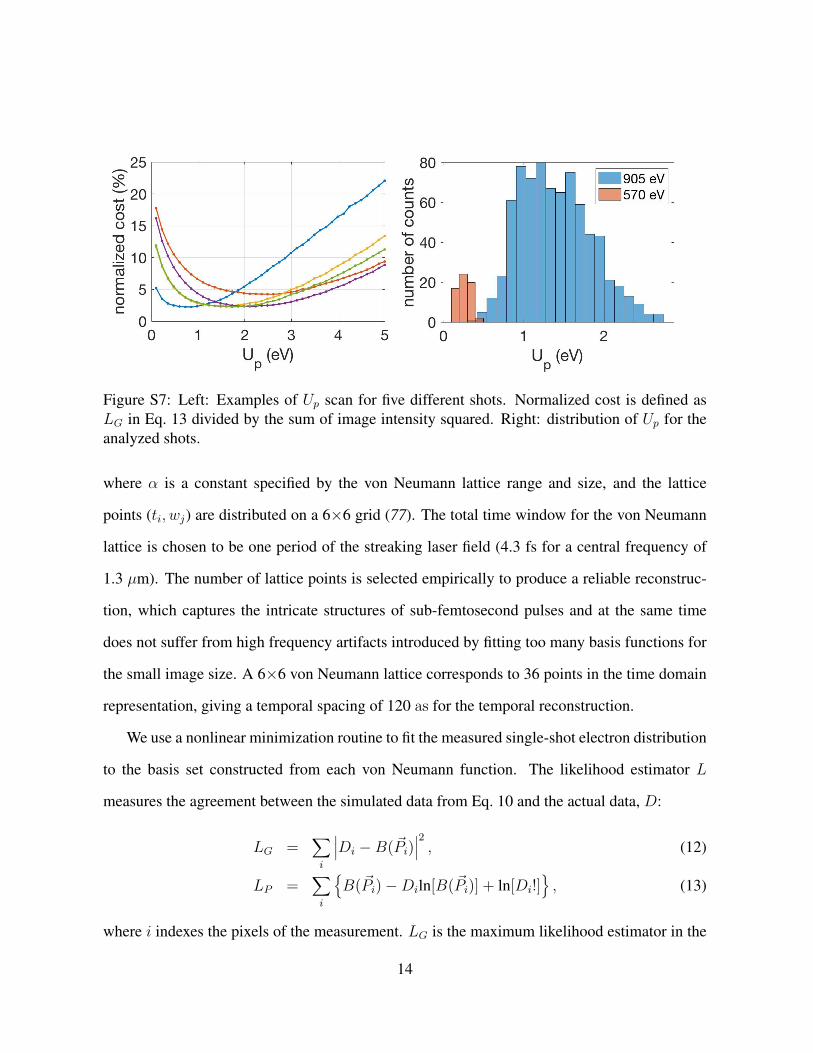
Figure S7: Left: Examples of Up scan for five different shots. Normalized cost is defined asLG in Eq. 13 divided by the sum of image intensity squared. Right: distribution of Up for theanalyzed shots.

where α is a constant specified by the von Neumann lattice range and size, and the lattice

points (ti, wj) are distributed on a 6×6 grid (77). The total time window for the von Neumann

lattice is chosen to be one period of the streaking laser field (4.3 fs for a central frequency of

1.3 µm). The number of lattice points is selected empirically to produce a reliable reconstruc-

tion, which captures the intricate structures of sub-femtosecond pulses and at the same time

does not suffer from high frequency artifacts introduced by fitting too many basis functions for

the small image size. A 6×6 von Neumann lattice corresponds to 36 points in the time domain

representation, giving a temporal spacing of 120 as for the temporal reconstruction.

We use a nonlinear minimization routine to fit the measured single-shot electron distribution

to the basis set constructed from each von Neumann function. The likelihood estimator L

measures the agreement between the simulated data from Eq. 10 and the actual data, D:

LG =∑

i

∣∣∣Di −B(~Pi)∣∣∣2, (12)

LP =∑

i

{B(~Pi)−Diln[B(~Pi)] + ln[Di!]

}, (13)

where i indexes the pixels of the measurement. LG is the maximum likelihood estimator in the

14

coun

ts (a

rb. u

nits

.)

Figure S8: Bandwidth distributions from spectrometer measurements at 905 eV (blue) andreconstructed shots from streaking measurements at 905 eV.

case of Gaussian distributed noise, whereas LP is the maximum likelihood estimator in the case

of Poisson distributed noise. Both likelihood estimators were tested and provide similar results.

Use of the von Neumann representation affords a sparse representation of the x-ray pulse, which

assists in the robustness of the nonlinear fitting routine.

As described above, the relative phase between the x-ray pulse and the streaking pulse

is random, and we do not have knowledge of the instantaneous value of the vector potential

amplitude, or the ponderomotive potential, Up, responsible for the momentum shift. As shown

in (75), we find the optimal Up by scanning the likelihood estimator, Eq. 13, as a function of

Up with a range from 0.5 to 5 eV. The likelihood estimator varies smoothly with Up, showing a

clear minimum which identifies the optimal Up (see Fig. S7).

The basis images (Eq. 10) are calculated on a 64 × 64 grid and downsized to 32×32 to

prevent numerical artifacts, and then convolved with a Gaussian filter with σ equivalent to the

convolution strength of 25 pixels on a 1024×1024 grid, to match the filtering performed on the

data.

The nonlinear fitting search is initiated by random numbers for the coefficients based on

15

0.5 1 1.5

RMS[fs]

RMS[eV]

0

50

100

150

200nu

mbe

r of

cou

nts

Figure S9: Distribution of time-frequency RMS bandwidth product of 905 eV data. The verticalblue line indicates the median of the distribution at 0.51.

Monte Carlo sampling. For each shot, we run 20 iterations of the reconstruction algorithm with

different initial values and check the convergence by comparing each solution. The time domain

profile of the x-ray field is given by,

EX(t) =∑

n

cnαn(t), (14)

where cn are the optimal coefficients returned by the algorithm. We then take the Fourier trans-

form of the time-domain x-ray field profile to obtain the spectral domain profile.

Note that the spectral domain is sensitive to spiky structures in the time domain profile

which are artifacts of the algorithm due to Poisson noise. To mitigate this problem, we apply a

Gaussian filter to the time domain field profile with a σt = 170 as for 570 eV and σt = 120 as

16

Figure S10: Distribution of pulse duration uncertainty as a function of pulse energy and streak-ing amplitude.

for 905 eV. The Gaussian filter width is comparable to the basis function lattice grid size

(120 as). With this Gaussian filter the statistical distribution of the FWHM bandwidth obtained

from the reconstruction closely matches the spectrometer data (see Fig. . S8), which provides

an independent benchmark for the reconstruction method.

Figure S9 shows the distribution of time-frequency bandwidth product measured from the

reconstructed pulses. For a Fourier-transform limited Gaussian pulse the time-frequency RMS

bandwidth product should be 0.32 and the average time-bandwidth product is within a factor

two of this value.

1.4.1 Quantification of the single-shot experimental uncertainty

The reconstruction algorithm can converge to different solutions for a given pulse due to the fi-

nite number of counts in each shot and the finite resolution of the VMI. These different solutions

all match the measured data very accurately, with an integrated error smaller than 3%. There-

fore we can employ the statistical distribution of these independent reconstructions to quantify

the most probable solution as well as the experimental uncertainty on the pulse profile and pulse

duration.

17

To obtain the most probable solution, we calculate the inner product between each of the 20

solutions (i.e. < Ii, Ij >with i, j = 1,2,...,20) for each shot. We then identify the most probable

solution as the one with the highest inner product, shown as the red curve in main text Fig. 2.

The standard deviation of the inner product of these solutions is a measure of the uncertainty on

the overall pulse profile and it has an average value of 6%.

To obtain an estimate of pulse duration uncertainty we calculate the standard deviation of the

pulse duration found by the 20 solutions. We define the uncertainty to be σ (∆τRMS)/∆τRMS,

where σ is the standard deviation. The median of the uncertainty distribution is 20% (28%) for

905 eV (570 eV). Figure S10 shows the pulse duration uncertainty correlates with the streaking

amplitude and the pulse energy, indicating that the uncertainty is smaller for higher streaking

amplitude as well as for higher pulse energy. The dependence on the streaking amplitude comes

from the decreasing angular resolution corresponding to small radius on the detector. In the

limiting case where the streaking amplitude is 0, there is complete degeneracy across the time

axis. The dependence on higher pulse energy can be explained by stronger signal.

2 Supplemental Text

2.1 Two-Color Pulse Properties

The characteristic intensity jitter of single-spike sub-fs FELs is also observed in the double-

pulse operation. Figure S11 (a) shows a scatter plot of the pulse energy contained in the two

pulses from shot-to-shot. The pulse energy in each pulse has close to 100% fluctuations, and

the intensities of the two pulses are anti-correlated, a well known property of the split undulator

method (78). This is because when running the system as close as possible to saturation, a large

increase in the energy of the first pulse spoils the energy-spread of the electron beam, causing

the second pulse to be weaker. One could improve the relative pulse stability at the cost of a

reduced peak power by interrupting the gain of the first pulse earlier and reducing the effect of

18

930 940 9500.02.5

Photon energy (eV)

Spect

ral in

tensi

ty (

uJ/eV

)

0 10 20 30936 eV pulse energy (uJ)

0

10

20

95

0 e

V p

uls

e e

nerg

y (

uJ)(a)

(c)

(b)

0.0 0.5 1.0936 eV pulse energy fraction

0

25

50

75

Num

ber

of

shots

Figure S11: Single-shot spectral measurements for the two-color experiment. (a) Single-shotmeasurement of the intensity of each pulse. (b) Representative single-shot spectra for the two-color setup. (c) Histogram of the fraction of the total pulse energy in each pulse.

the first pulse on the second.

Figure S11 (b) shows a few examples of single shot two-color spectra, while Fig. S11 (c)

is a histogram of the relative intensities of the two pulses. While the source has significant

intensity jitter, the pulse energy is so large that the properties can be measured on a single-shot

basis for all the shots with non-destructive diagnostics. Therefore one could apply this method

to time-resolved pump/probe experiments and sort the data based on single-shot measurements

of the pulse properties.

2.2 Machine Parameter Correlations

We have examined the correlation between the retrieved pulse durations and a number of critical

machine parameters: the peak electron beam current measured at bunch compressors 1 and 2

(BC1 and BC2) and the electron beam energy after acceleration. Figure S12 shows that there

is no clear correlation between either of these parameters and the measured pulse duration (the

19

Figure S12: Scatter plots of machine parameters and the retrieved pulse durations. The bluedots are for the neon data at 905 eV, and red for the CO2 data at 570 eV.

calculated correlation coefficients are all below 0.2).

References

65. R. Bonifacio, C. Pellegrini, L. Narducci, Optics Communications 50, 373 (1984).

66. J. MacArthur, et al., Submitted to Phys. Rev. Lett. (2019).

67. Y. Ding, Z. Huang, D. Ratner, P. Bucksbaum, H. Merdji, Phys. Rev. ST Accel. Beams 12,

060703 (2009).

68. E. L. Saldin, E. A. Schneidmiller, M. V. Yurkov, Phys. Rev. ST Accel. Beams 9, 050702

(2006).

69. P. Baxevanis, J. Duris, Z. Huang, A. Marinelli, Phys. Rev. Accel. Beams 21, 110702 (2018).

70. C. Behrens, et al., Nat Commun 5 (2014).

71. S. Li, et al., AIP Advances 8, 115308 (2018).

20

72. J. M. Glownia, et al., Optics Express 18, 17620 (2010).

73. S. Moeller, et al., Nuclear Instruments and Methods in Physics Research Section A: Accel-

erators, Spectrometers, Detectors and Associated Equipment 635, S6 (2011).

74. R. Storn, K. Price, Journal of Global Optimization 11, 341 (1997).

75. S. Li, et al., Optics Express 26, 4531 (2018).

76. M. Kitzler, N. Milosevic, A. Scrinzi, F. Krausz, T. Brabec, Physical Review Letters 88,

173904 (2002).

77. S. Fechner, F. Dimler, T. Brixner, G. Gerber, D. J. Tannor, Optics Express 15, 15387 (2007).

78. A. A. Lutman, et al., Phys. Rev. Lett. 110, 134801 (2013).

21