Tukey’s Biweight Correlation and the Breakdown

Mary Owen

April 2, 2010

2

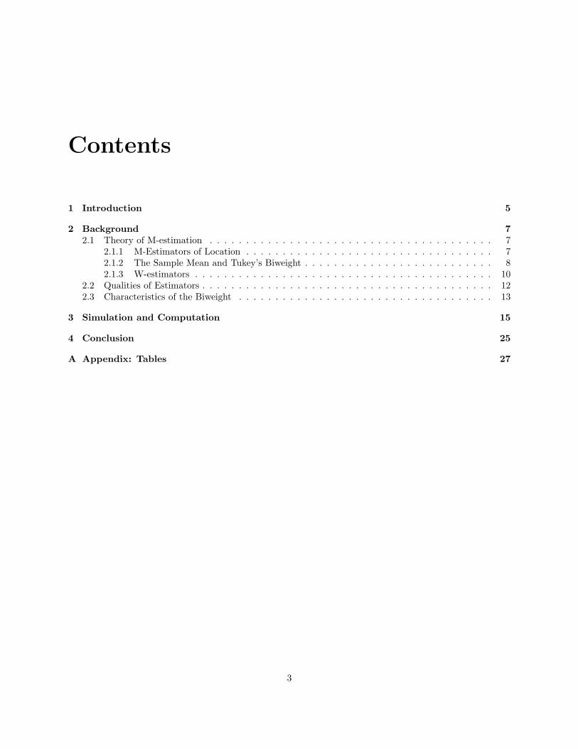
Contents

1 Introduction 5

2 Background 72.1 Theory of M-estimation . . . . . . . . . . . . . . . . . . . . . . . . . . . . . . . . . . . . . . . 7

2.1.1 M-Estimators of Location . . . . . . . . . . . . . . . . . . . . . . . . . . . . . . . . . . 72.1.2 The Sample Mean and Tukey’s Biweight . . . . . . . . . . . . . . . . . . . . . . . . . . 82.1.3 W-estimators . . . . . . . . . . . . . . . . . . . . . . . . . . . . . . . . . . . . . . . . . 10

2.2 Qualities of Estimators . . . . . . . . . . . . . . . . . . . . . . . . . . . . . . . . . . . . . . . . 122.3 Characteristics of the Biweight . . . . . . . . . . . . . . . . . . . . . . . . . . . . . . . . . . . 13

3 Simulation and Computation 15

4 Conclusion 25

A Appendix: Tables 27

3

4

Chapter 1

Introduction

DNA microarray experiments have become increasingly popular in recent years as a method of uncoveringpatterns of gene expression and relationships between genes. Though sometimes problematic, it is possible todivide genes into groups based on the similarity of their patterns of expression, measured with any of severaldifferent measures of similarity, the Pearson correlation being the most popular [4]. With the measureof similarity determined, a clustering algorithm or gene network analysis can give more insight into therelationship between the genes.

However, the similarity measure will have a large impact on the clustering algorithm. If the similaritymeasure is not resistant enough to outliers and noise in the data, dissimilar genes may be clustered asthough they are co-expressed, or vice versa. Microarray data tend to contain a lot of noise, which cancome from many different sources over the course of a microarray experiment and may remain in the datadespite normalization or filtering [7, 6]. For accurate results, a robust measure of similarity is needed. In a2007 paper, Hardin et al. proposed a resistant correlation measure for use in clustering and gene networkalgorithms. This new correlation measure is based on Tukey’s biweight and can be used both in clusteringand gene network algorithms and, by comparing it with the Pearson correlation, as a method of flaggingquestionable data points. It is more resistant than the Pearson correlation and more efficient than theSpearman correlation [4].

Despite having performed promisingly so far, there is still much to learn about the biweight correlation. Itis somewhat unusual in that its breakdown point, defined in section 2.3, can be set to a specified value. In thispaper, we will explore the performance of the biweight correlation under a variety of different experimentalconditions in order to determine how the biweight correlation varies as its breakdown point changes. Fordifferent breakdown points, underlying distributions of the data, and sample sizes, we will compute theefficiency and bias. We will compare the performance of the biweight to that of the Pearson correlationunder identical circumstances with the goal of finding the best similarity measure.

5

6

Chapter 2

Background

2.1 Theory of M-estimation

2.1.1 M-Estimators of Location

The original development of M-estimators of location was based on creating robust estimators similar toMaximum Likelihood Estimators (MLEs). Because some M-estimators are robust, that is, not overly affectedby outliers, they are wonderful tools to use in the analysis of microarray data, which is often full of outliersand noise. M-estimators of location are independent of the underlying probability distribution function ofthe data because they minimize an objective function that is dependent on the distances from the observedvalues to the estimate. Since microarray data is multivariate - that is, for each person we know about theexpression of multiple genes - we will consider each observation to be a vector, X. Most of the theory thatapplies to M-estimators of location in one dimension can be generalized to multivariate data. For a functionρ(Xi, t), called the objective function, and a sample X1, . . . , Xn, the M-estimator of location Tn(X1, . . . , Xn)is the value of t that minimizes

n∑i=1

ρ(Xi, t) (2.1)

When ρ is continuous and has a derivative with respect to t, we call that derivative the M-estimator’sψ-function and simplify the calculation of the M-estimator by computing a value of t such that

n∑i=1

ψ(Xi, t) = 0 (2.2)

For the M-estimators of location with which we are concerned, ρ is independent of the underlying distributionof the data. If ρ = f , the pdf of the distribution, then the M-estimator is the MLE. [5]

We would like any M-estimator of location to be location-and-scale-equivariant, that is, we would like it torespond in a reasonable manner to linear changes across the sample. An M-estimator is location equivariantif, when every observation is shifted by some amount C, the Tn of that shifted sample also shifts by C.An M-estimator of location is scale equivariant if, when every observation is multiplied by some nonzeroconstant d, the Tn of that altered sample is d times the Tn of the unaltered sample. An M-estimator oflocation that possesses both these characteristics is location-and-scale equivariant. In other words, we wantthe following to hold:

Tn(dX1 + C, dX2 + C, . . . , dXn + C) = dTn(X1 +X2 + · · ·+Xn) + C (2.3)

In order for an M-estimator of location to be location-and-scale-equivariant, it is often necessary to scale theobservations when computing ρ and ψ. This is often done whether rescaling is necessary or not because itmakes notation simpler. The matter of location-equivariance is fairly simple; it can be satisfied by making

7

the input of the form X − Tn. Adjusting for scale is not as straightforward. We must pick some estimatorof the scale of the sample, called Sn, which is a function of the observations X1, X2, . . . , Xn. Sn is scale-equivariant and location invariant, meaning that it is unaffected by a shift in the sample as described above[5]. For our multivariate microarray data, the observations are transformed to

ui = (Xi − Tn)t(cSn)−1(Xi − Tn) (2.4)

where Tn is a location vector and Sn is a shape matrix. In one dimension, the observations are transformedto

ui =xi − TncSn

(2.5)

where Tn and Sn are location and shape scalars, and c is a tuning constant. Note that regardless of thedimensional of the data, the ui will be one-dimensional. Equation (2.1) now becomes

n∑i=1

ρ(ui) (2.6)

and Equation (2.2) becomesn∑i=1

ψ(ui) = 0 (2.7)

where Tn and Sn that solve equation (2.7) are the resulting M-estimates of location and shape, respectively.

2.1.2 The Sample Mean and Tukey’s Biweight

The simplest example of an M-estimator is the least squares estimator of the sample mean in one dimension.In this case, we wish to minimize the sum of the squared residuals, the distances between the observationsand the estimator. Thus,

ρ(x, t) = ((x− t)cS

)2

and we minimize

n∑i=1

((xi − t)cS

)2

or, after differentiating to simplify the calculation, solve the equation

n∑i=1

(xi − t

)= 0

The value of t that solves this is the sample mean, Tn =∑ni=1 xi/n. It is straightforward to show that the

sample mean is location-and-scale equivariant.Unfortunately, the sample mean is not robust. Outliers can skew the estimate of the sample mean enough

so that it is no longer helpful as an analysis tool. To find a robust estimator, we turn to a different familyof ρ functions. Statisticians have developed many robust M-estimators, but in this paper we are concernedwith one in particular: Tukey’s biweight. The biweight estimate of correlation is produced by first iterativelycalculating the biweight estimate of shape, S. The (i, j)th element of S, sij , can be thought of as a resistantestimate of the covariance between two vectors, Xi and Xj . The biweight correlation of these two vectors iscalculated as follows:

rij =sij√siisjj

(2.8)

8

This is very similar to the calculation of the Pearson correlation, given in equation (2.11). The biweighthas the objective function

ρ(u) ={

16

[1− (1− u2)3

]if |u| ≤ 1

16 if |u| > 1 (2.9)

and ψ-function

ψ(u) ={u(1− u2)2 if |u| ≤ 10 if |u| > 1 (2.10)

where u = x−Tn

cSnas in equation (2.5) [5].

−2 −1 0 1 2

−0.

3−

0.2

−0.

10.

00.

10.

20.

3

u

psi(u

)

Figure 2.1: The ψ-function for the biweight M-estimator.

9

−2 −1 0 1 2

0.00

0.05

0.10

0.15

u

rho(

u)

Figure 2.2: The objective function for the biweight M-estimator.

As you can see in Figure 2.1, the ψ-function redescends to zero, that is, if |u| is large enough, ψ(u) = 0.Since the ψ-function determines the weights assigned to the data points, as we will see in Section 2.1.3, pointswith large values of u do not effect the calculation of the biweight estimate. This means that the biweightis less affected by outliers than estimates based on the least squares function. In addition, the ψ-functionis linear at u = 0 in accordance with Winsor’s principle that all distributions are normal in the middle [3].This means that ψ(u)

u is constant over the linear region of ψ, so the points in that region all get equal weight.The biweight estimate of correlation has been proposed as a basis for the measure of similarity used

in microarray analysis [4]. However, the biweight is computationally intensive, so the Pearson correlation(hereafter referred to as Pearson) is more commonly used in clustering microarrays. Pearson is also theaccepted gold standard for use on normally distributed data. For bivariate data with variables X and Y ,it is calculated by finding the covariance of X and Y and dividing by the square root of the product of thevariances, as follows [1]:

Pearson =∑ni=1 (Xi − X)(Yi − Y )√∑n

i=1 (Xi − X)2∑ni=1 (Yi − Y )2

(2.11)

Unlike the biweight, Pearson weighs each point equally, so it is not robust to outliers, as we shall see.

2.1.3 W-estimators

While M-estimates exist in theory, solutions to the optimization problem do not usually exist in closedform. To find a solution, we turn instead to iteratively calculated W-estimators, which often give a closeapproximation to the true M-estimate solution. Combining equations (2.4) and (2.7), we see that the M-estimator of location Tn and the M-estimator of scale Sn are those values which solve the following equation:

n∑i=1

ψ(Xi − Tn)t(Sn)−1(Xi − Tn) = 0 (2.12)

Let us define the equation w(u) = ψ(u)u and substitute into equation (2.12). We can then solve for Tn

and for Sn, obtaining,

10

Tn =∑ni=1Xiw(ui)∑ni=1 w(ui)

(2.13)

Sn =∑ni=1 w(ui)(Xi − T )(Xi − T )t∑n

i=1 w(ui)(ui)(2.14)

By using w(u), we have turned Tn into a weighted M-estimate, called a W-estimate. However, typicallyclosed-form solutions to equations (2.13) and (2.14) also do not exist. We can iteratively calculate Tn andSn to find a close approximation of the solution. We iteratively calculate the values of u that we use toobtain Tn and Sn in the following manner. If T (k)

n and S(k)n are the M-estimates given at the kth iteration,

then the u(k)i = (Xi−T (k)

n )t(S(k)n )−1(Xi−T (k)

n ) are the rescaled data points that we will use to calculate Tnand Sn for the (k + 1)th iteration as follows:

T (k+1)n =

∑ni=1Xiw[u(k)

i ]∑ni=1 w[u(k)

i ](2.15)

S(k+1)n =

∑ni=1 w(u(k)

i )(Xi − T (k+1))(Xi − T (k+1))t∑ni=1 w(u(k)

i )(u(k)i )

(2.16)

The weights for a particular T (k)n and S(k)

n depend upon the previous values, T (k−1)n and S(k−1)

n [5]. Thebenefit of this iterative procedure is that it can be solved for values of Tn and Sn that, in most cases, convergeto the solutions of the objective function. We simply start with a reasonable guess of the values of Tn andSn and iterate until the estimates have converged to within whatever we consider to be a reasonable marginof accuracy, that is, until

∣∣∣∣∣∣T (k+1)n − T (k)

n

∣∣∣∣∣∣ and∣∣∣∣∣∣S(k+1)

n − S(k)n

∣∣∣∣∣∣ are less than some predecided values [9].This procedure is an example of the process of iteratively reweighted least squares (IRLS).

IRLS can have some negative effects when used with Tukey’s biweight. The weight function of Tukey’sbiweight is

w(u) ={

(1− u2)2 if |u| ≤ 10 if |u| > 1 (2.17)

and its graph is shown in Figure 2.3. Like the ψ-function, the weight function redescends to zero. Aconsequence of this is that if a point is sufficiently far away from the main body of the data, it will be givena weight of zero and will not enter into the calculation of the biweight estimate at all. However, when IRLSis employed, more and more points can be “eliminated” from the data set with each iteration. At eachstep, the most extreme outliers are dropped from the sample because they are outside of a certain mainbody of the data, determined by the covariance matrix, S(k)

n . As outlying or extreme values are eliminated,S

(k)n decreases, u(k)

i increases, and with each iteration more points are dropped. Left unchecked, IRLS cansometimes give zero weight to every point and whittle the data set away to nothing, so IRLS estimatorsneed constraints applied to them that will counteract the effect of the redescending weight function. Theconstraints take the following form:

1n

∑i

ρ(ui) = b0

b0 = E(ρ(u))

To calculate b0 we assume that the data are normally distributed and use the moment generating functionto find E[ρ(u)]. Such constrained estimators are called S-estimators [3].

11

−2 −1 0 1 2

0.0

0.2

0.4

0.6

0.8

1.0

u

w(u

)

Figure 2.3: The weight function for the biweight M-estimator.

2.2 Qualities of Estimators

Ideally, we would like our estimator to be both robust and resistant. An M-estimator is said to be robustif changes in the underlying distribution of the data have little effect on the estimator’s value [9]. AnM-estimator is resistant if a change in a small part of the data produces little change in the value of theestimator. Resistant estimators focus on the main body of the data and pay little attention to outlyingpoints [5].

The sensitivity curve and the influence curve are useful tools for examining the resistance of an estimatorwhen working with one-dimensional data. The concepts can be intuitively expanded to multiple dimensions,although solutions would likely not be in a closed form. For the remainder of this section, we will be speakingabout M-estimations of location found on one-dimensional data. The sensitivity curve shows how changinga particular sample by one observation would affect an estimator. For a sample of size n and an estimatorTn, the sensitivity curve can be expressed as a function of the nth observation, x:

SC(x;x1, . . . , xn−1, Tn) = n{Tn(x1, . . . , xn−1, x)− Tn−1(x1, . . . , xn−1)} (2.18)

Note that for a given sample and estimator, the sensitivity curve depends only on the extra observationx [5]. We wish the sensitivity curve to be bounded because that indicates that there is no value of x that,when added to the sample, could cause the estimator Tn to go over all bounds.

However, the sensitivity curve, while realistic, is not the most useful tool for describing an estimatorbecause it is dependent on a particular sample. To get more information about the estimator itself, weconsider an asymptotic version of the sensitivity curve as n goes to infinity. This is called the influencefunction. The influence function describes the effect of a proportionate change ε of contamination in adistribution F on an estimator T . The influence function is defined as follows

IF (x;F, T ) = limε→0

T ((1− ε)F + εδx)− T (F )ε

(2.19)

12

if the limit exists [5]. Similarly to the sensitivity curve, we find the difference between the estimate withuncontaminated data, T (F ), and the estimate based on the same distribution with a fraction ε of theobservations being contaminated, where δx is a distribution with all its mass at the point x [8]. For one-dimensional M-estimators of location, it can be shown that the influence function is a constant multiple ofthe ψ-function, that is,

IF (T ) = a · ψT (u). (2.20)

for some constant a. For a given influence funtion, it is possible to find an accompanying ψ-function thatfulfills equation (2.20) [5].

The influence function provides us with a measure of resistance called the gross error sensitivity (g.e.s.).The g.e.s. is the maximum effect that a small contamination can have on an estimator and it is given by

γ∗ = supx|IF (x;F, T )|. (2.21)

For a resistant estimator, γ∗ must be bounded, and in general we would like it to be as small as possible[8].

Both the influence and sensitivity curves depend on having some knowledge of the data, be it the actualsample values in the case of the sensitivity curve, or the underlying distribution of the data set in the caseof the influence curve. For the purposes of this paper, we will simulate our experimental data, so we knowthe underlying distribution. For actual microarray data, distributions are unknown, and because the dataare so often full of noise, the knowledge of one point’s effect on the biweight estimator is not very useful.

2.3 Characteristics of the Biweight

In the computational section of this paper, we will examine several characteristics of the biweight correlation.The one that concerns us the most is the breakdown.

There are two different types of breakdown, the replacement breakdown and the additive breakdown.The replacement breakdown describes how well an estimator performs when at least one of the original datapoints has been replaced with an arbitrary value. The additive breakdown describes how well an estimatorperforms when we have added random data to the original data set. In this paper, we are concerned with thereplacement breakdown, hereafter referred to simply as the breakdown, or breakdown point. The breakdownpoint of an M-estimator Tn is “the smallest fraction m

n of outliers that can take the estimator over allbounds” [3]. In other words, it is “the smallest fraction of contamination that can cause the estimator T totake on values arbitrarily far away from Tn” [8]. For example, the breakdown point for the sample meanis 1

n because if even one point becomes arbitrarily large, so does the sample mean. For S-estimators, themaximum possible breakdown is b(n−p)/2cn , which approaches 1

2 as n → ∞ [3]. Note that the breakdownpoint does not depend on the underlying distribution of the data. It is essential to keep in mind that while ahigh breakdown is a good indicator of resistance, it is not a guarantee that an estimator won’t be influencedby outliers [9].

We are also concerned with the efficiency of an M-estimator. The typical measure of efficiency is basedon the Cramer-Rao inequality. An estimator T of a parameter θ is efficient if it attains the Cramer-Raolower bound, defined as

V ar(T ) =( ddθE(T ))2

nE[ ddθ ln f(x)]2(2.22)

where f(x) is the probability distribution function of the distribution from which the sample is drawn[2]. However, the Cramer-Rao definition does not apply here because the algebra involved in making thecalculation for our multivariate data would be nearly impossible. Additionally, it is unlikely that anyestimator of correlation (the statistic of interest) would actually attain the Cramer-Rao lower bound. Thus,we must find a working definition of efficiency that is useful in our situation. One estimator is more efficient

13

than another if its variance is smaller, which typically means that its mean squared error is smaller andit produces a smaller confidence interval. In our work we will use the standard technique of calculatingefficiency as the ratio of the empirical variance of the biweight correlation to the empirical variance of thePearson correlation.

We will also find the empirical bias of the biweight and Pearson estimators. DeGroot and Schervish definethe bias of an estimator as “The difference between the expectation of an estimator and the parameter θthat is being estimated” [2]. In our work, since we are simulating bivariate data, we can set the measureof correlation between the two variables, ρ, to be whatever we choose, so we know the true value of ρ andcan compare it to the expected values of the different estimators. We estimate the expected values usingthe empirical expected values. This is possible because of the law of large numbers, which states that thesample mean converges in probability to the true mean as n increases [2].

14

Chapter 3

Simulation and Computation

All calculations were performed using the software R, version 2.10.0, and the biweight was calculated using thepackage biwt developed by Hardin [4]. Four estimators were chosen for comparison: the Pearson correlation,and Tukey’s biweight with the breakdown set to 0.1, 0.2, and 0.4. They were compared on simulated bivariatedata sets with a set true correlation value (ρ) over three different types of distributions: standard normal,standard normal with one randomly generated extreme outlier (one-wild), and standard normal with 20%of the data points randomly selected to be removed and replaced with randomly generated extreme outliers(random 20). The outliers were created by randomly picking two numbers from the interval [−50, 50]. Thefour estimates were calculated 500 times for every possible combination of these three distributions, threedifferent values of the true correlation (ρ = 0.3, 0.5, 0.8), and four different sample sizes (n = 20, 50, 100, 500).For each estimate, the mean and standard deviation of the correlation were calculated over the 500 repetitions.

First, let us examine the empirical results. Figure 3.1 displays the estimates of correlation for all standardnormal data with a true correlation value of 0.8; that is, what is shown encompasses all four sample sizes.Each row and each column belong to an estimator. From top to bottom and left to right, the order of plotpanels is biweight with r = 0.1, biweight with r = 0.2, biweight with r = 0.4 and Pearson. The histogramsshow the distribution of each of the estimates given by a particular estimator, and each histogram represents2, 000 data points from 500 repetitions over four sample sizes. The histograms also have vertical lines at0.8 on the x-axis, marking the true correlation value. The numbers in the upper right triangle show thecorrelation between estimators. The scatterplots in the lower left triangle show the relationship of twoestimators plotted against each other.

For standard normal data, the scatterplots show that the estimators are generally very similar to eachother. All four are biased but have extremely small biases (Table A.1). The Perason correlation estimator iswell known to be biased, so detecting a bias here is no surprise. Pearson and the biweight with r = 0.1 areremarkably similar, with a correlation of 0.99. This is a very good sign because, as mentioned previously,Pearson is widely considered the best estimate of correlation for normally distributed data. The biweightwith r = 0.4 is the least efficient of the three for normal data under all correlations and sample sizes, as canbe seen in Table A.2. This is because it is effectively working with a smaller sample size than the other threeestimators. With a breakdown of r, the biweight is essentially ignoring r(100)% of the data and only givingan estimate based on (1− r)100% of the available observations.

Sample size has a large effect on the performance of the estimators. Figure 3.2 shows only the 500repetitions performed with a sample size of n = 20. All four histograms have much longer left tails thanthey did in Figure 3.1, and the points in the scatterplots are spread widely. However, when we look atthe simulation with a sample size of n = 500 in Figure 3.3, the performance of every estimator improvesdrastically, as expected. The biweight with a breakdown of r = 0.2 is now even closer to successfullyapproximating Pearson, producing results that have a correlation of 0.95 with Pearson’s estimates.

15

Biwt0.1

0.4 0.6 0.8 1.0

0.98 0.76

0.4 0.6 0.8 1.0

0.4

0.6

0.8

1.0

0.99

0.4

0.6

0.8

1.0

Biwt0.2

0.84 0.95

Biwt0.4

0.4

0.6

0.8

1.0

0.70

0.4 0.6 0.8 1.0

0.4

0.6

0.8

1.0

0.4 0.6 0.8 1.0

Pearson

Normal Data, rho = 0.8

Figure 3.1: Estimates of a true correlation value of 0.8 over a range of sample sizes (n = 20, 50, 100, 500) forstandard normal bivariate data.

Biwt0.1

0.4 0.6 0.8 1.0

0.97 0.73

0.4 0.6 0.8 1.00.

40.

60.

81.

0

0.99

0.4

0.6

0.8

1.0

Biwt0.2

0.82 0.95

Biwt0.4

0.4

0.6

0.8

1.0

0.67

0.4 0.6 0.8 1.0

0.4

0.6

0.8

1.0

0.4 0.6 0.8 1.0

Pearson

Normal Data, rho = 0.8, n = 20

Figure 3.2: Estimates of a true correlation value of 0.8 for standard normal bivariate data and a sample sizeof 20.

16

Biwt0.1

0.75 0.80 0.85

0.98 0.81

0.75 0.80 0.85

0.75

0.85

0.99

0.75

0.85 Biwt0.2

0.89 0.95

Biwt0.4

0.75

0.85

0.74

0.75 0.80 0.85

0.75

0.85

0.75 0.80 0.85

Pearson

Normal Data, rho = 0.8, n = 500

Figure 3.3: Estimates of a true correlation value of 0.8 for standard normal bivariate data and a sample sizeof 500.

Figure 3.4 displays the estimates of correlation for all one-wild data with a true correlation value of0.8. The histograms indicate that even with just one random outlier inserted into the normal data, Pearsonhas lost its efficiency, and it is now extremely biased, much less efficient, and completely uncorrelated withall three biweights. In fact, Pearson gives an average true corrlation estimate of 0.169, a far cry from theexpected value of 0.8. Clearly the Pearson correlation estimator is not robust to even a single extreme outlier.

When we compare the one-wild data for sample sizes of n = 20 and n = 500, the differences are striking.With the smaller sample size, the histograms and scatterplots in Figure 3.5 bear a strong resemblance tothose in Figure 3.4. But when the sample size is increased to 500, the biweight becomes much more accurateand efficient under all three breakdowns, while Pearson continues to perform dismally. That is, even with asample size of n = 500, even one rogue observation can ruin the Pearson estimate. For the one-wild data, thebiweight with r = 0.1 is consistently most efficient and often most accurate, making it the best of these fourestimators for data with one extreme outlier. This is probably because, as proposed earlier, it is workingwith an effective sample size of 90% of n, rather than 80% or %60 of n.

17

Biwt0.1

−1.0 −0.5 0.0 0.5 1.0

0.97 0.77

−1.0 −0.5 0.0 0.5 1.0

−1.

00.

01.

0

0.0096

−1.

00.

01.

0Biwt0.2

0.85 0.011

Biwt0.4

−1.

00.

01.

0

0.008

−1.0 −0.5 0.0 0.5 1.0

−1.

00.

01.

0

−1.0 −0.5 0.0 0.5 1.0

Pearson

One−wild Data, rho = 0.8

Figure 3.4: Estimates of a true correlation value of 0.8 over a range of sample sizes (n = 20, 50, 100, 500) forone-wild bivariate data.

Biwt0.1

−1.0 −0.5 0.0 0.5 1.0

0.96 0.75

−1.0 −0.5 0.0 0.5 1.0−

1.0

0.0

1.0

0.013

−1.

00.

01.

0

Biwt0.2

0.84 0.0091

Biwt0.4

−1.

00.

01.

0

0.011

−1.0 −0.5 0.0 0.5 1.0

−1.

00.

01.

0

−1.0 −0.5 0.0 0.5 1.0

Pearson

One−wild Data, rho = 0.8, n = 20

Figure 3.5: Estimates of a true correlation value of 0.8 for one-wild bivariate data and a sample size of 20.

18

Biwt0.1

−1.0 −0.5 0.0 0.5 1.0

0.99 0.83

−1.0 −0.5 0.0 0.5 1.0

−1.

00.

01.

0

0.037

−1.

00.

01.

0Biwt0.2

0.90 0.033

Biwt0.4

−1.

00.

01.

0

0.0067

−1.0 −0.5 0.0 0.5 1.0

−1.

00.

01.

0

−1.0 −0.5 0.0 0.5 1.0

Pearson

One−wild Data, rho = 0.8, n = 500

Figure 3.6: Estimates of a true correlation value of 0.8 for one-wild bivariate data and a sample size of 500.

Figure 3.7 displays the estimates of correlation for all data that began with a true correlation value of 0.8and has been altered by randomly replacing 20% of the data points with outliers. From the histograms, itappears that the estimates given by Pearson and the biweight with r = 0.1 are normally distributed aroundzero. In fact, for Pearson the empirical mean is 0.002 and the empirical mean of that biweight is 0.018. Thesetwo estimators are very biased for the random 20 data. The biweight with r = 0.2 gives more estimates thatare close to 0.8, but the mean value of correlation for that breakdown is 0.530. This is somewhat surprising.With a breakdown of 0.2, the biweight should be able to successfully ignore the 20% of the data that areoutliers, but its performance is very dependent on sample size, as we will see. The biweight with r = 0.4,however, is a stellar performer. It is both accurate and efficient, with a bias of only 0.0082 (Table A.1). Fordata with 20% outliers, it is clearly the best of the three.

Once again, sample size makes a big difference in the performance of the estimators, although the break-down with r = 0.4 is the still the best of the four. When the sample size is only 20, as in Figure 3.8, thehistogram for the Pearson estimator appears almost uniform, and the biweights with breakdowns of r = 0.1and r = 0.2 are so heavy-tailed that their histograms are U-shaped. When the sample size is increased to500, as in Figure 3.9, the performance of the biweight with r = 0.2 improves dramatically - its bias nearszero and its efficiency nears one - although it still cannot touch the biweight with r = 0.4 (see Tables A.1and A.2. Perhaps if n becomes big enough, the breakdown that we set will accurately reflect the practicalbreakdown. This could be a topic for further investigation.

19

Biwt0.1

−1.0 −0.5 0.0 0.5 1.0

0.18 0.044

−1.0 −0.5 0.0 0.5 1.0

−1.

00.

01.

0

0.80

−1.

00.

01.

0Biwt0.2

0.13 0.12

Biwt0.4

−1.

00.

01.

0

0.015

−1.0 −0.5 0.0 0.5 1.0

−1.

00.

01.

0

−1.0 −0.5 0.0 0.5 1.0

Pearson

Random 20 Data, rho = 0.8

Figure 3.7: Estimates of a true correlation value of 0.8 over a range of sample sizes (n = 20, 50, 100, 500) forrandom 20 bivariate data.

Biwt0.1

−1.0 −0.5 0.0 0.5 1.0

0.23 0.062

−1.0 −0.5 0.0 0.5 1.0−

1.0

0.0

1.0

0.80

−1.

00.

01.

0

Biwt0.2

0.10 0.17

Biwt0.4

−1.

00.

01.

0

0.014

−1.0 −0.5 0.0 0.5 1.0

−1.

00.

01.

0

−1.0 −0.5 0.0 0.5 1.0

Pearson

Random 20 Data, rho = 0.8, n = 20

Figure 3.8: Estimates of a true correlation value of 0.8 for random 20 bivariate data and a sample size of 20.

20

Biwt0.1

−0.5 0.0 0.5 1.0

0.054 0.017

−0.5 0.0 0.5 1.0

−0.

50.

51.

0

0.90

−0.

50.

51.

0Biwt0.2

0.15 0.035

Biwt0.4

−0.

50.

51.

0

0.007

−0.5 0.0 0.5 1.0

−0.

50.

51.

0

−0.5 0.0 0.5 1.0

Pearson

Random 20 Data, rho = 0.8, n = 500

Figure 3.9: Estimates of a true correlation value of 0.8 for random 20 bivariate data and a sample size of500.

Figures 3.10, 3.11 and 3.12 (see Appendix) plot sample size versus bias for all four estimators and allthree correlation sizes. The leftmost plots are all on the same y-axis scale for ease of comparison betweendistributions. Each color of dot represents a different estimator, and the three dots of each color for eachsample size are the biases of that estimator for each value of ρ. The normal data (Figure 3.10) shows aclear trend of bias decreasing as sample size increases. The position of the dots for n = 50 is probably dueto sampling error. Figure 3.11 shows the same trend. Even Pearson, which is wildly inaccurate comparedto the three biweights, improves as the sample size increases. Figure 3.12 demonstrates that Pearson andthe biweight with r = 0.1 never become less biased because they simply cannot handle the proportion ofoutliers in the data. The biweight with r = 0.4 has a very small bias for all four sample sizes. The biweightwith r = 0.2 actually becomes less biased as the sample size increases, although it is more biased thanthe biweight with r = 0.4 in every case. Perhaps with a large enough sample size the practical breakdownwould accurately reflect the theoretical breakdown and this biweight would be able to perform well with 20%random data.

21

●●●●●● ●●● ●●●

100 200 300 400 500

−0.

8−

0.6

−0.

4−

0.2

0.0

Normal Data

Sample Size

Bia

s●●● ●●● ●●● ●●●●●●

●●● ●●● ●●●●●●

●●● ●●● ●●●

●

●

●

●

biwt 0.1biwt 0.2biwt 0.4Pearson

●

●

●

●

●

●

●

●

●

●

●●

100 200 300 400 500

−0.

020

−0.

015

−0.

010

−0.

005

0.00

00.

005

Normal Data

Sample SizeB

ias

●

●

●

●

●

●

●

●

●

●

●●

●

●

●

●

●

●

●

●

●

●

●●

●

●

●

●

●

●

●

●

●

●

●●

●

●

●

●

biwt 0.1biwt 0.2biwt 0.4Pearson

Figure 3.10: Bias on normal data for all four estimators, all four sample sizes. Left: a larger y-axis scale forcomparison to other distributions. Right: a magnified scale for comparison between estimators for normaldata.

●●● ●●● ●●● ●●●

100 200 300 400 500

−0.

8−

0.6

−0.

4−

0.2

0.0

One−wild Data

Sample Size

Bia

s

●

●● ●●● ●●● ●●●

●

●● ●●● ●●● ●●●

●

●

●

●

●

●

●

●

●

●

●

●

●

●

●

●

biwt 0.1biwt 0.2biwt 0.4Pearson

●

●

●

●

●

●

●

●

●

●

●●

100 200 300 400 500

−0.

025

−0.

015

−0.

005

0.00

0

One−wild Data without Pearson

Sample Size

Bia

s

●

●

●

●

●

●

●●

●

●

●

●

●

●

●

●

●

●

●

●

●

●

●

●

●

●

●

biwt 0.1biwt 0.2biwt 0.4

Figure 3.11: Bias on one-wild data for all four estimators, all four sample sizes. Left: all four estimators ona larger y-axis scale for comparison to other distributions. Right: the three biweights on a magnified scale.

22

●

●

●

●

●

●

●

●

●

●

●

●

100 200 300 400 500

−0.

8−

0.6

−0.

4−

0.2

0.0

Random 20 Data

Sample Size

Bia

s

●

●

●

●

●

●

●●●

●●●

●●

● ●●● ●●● ●●●

●

●

●

●

●

●

●

●

●

●

●

●

●

●

●

●

biwt 0.1biwt 0.2biwt 0.4Pearson

● ●

●

●100 200 300 400 500

−0.

25−

0.20

−0.

15−

0.10

−0.

050.

000.

05

Random 20 Data

Sample Size

Bia

s

●

●

●

●

●●

●

●●

●

●

●

●●

●●

●●● ●●●

●● ●

●

●

●

●

●

biwt 0.1biwt 0.2biwt 0.4Pearson

Figure 3.12: Bias on random 20 data for all four estimators, all four sample sizes. Left: all four estimatorson a larger y-axis scale for comparison to other distributions. Right: note that the bias of the biweight withr = 0.2 approaches that of the biweight with r = 0.4 as n increases.

23

24

Chapter 4

Conclusion

We have seen that the Pearson correlation hardly deserves its stellar reputation for performance on normallydistributed data, since the biweight with r = 0.1 so closely matches it. However, the Pearson correlationdoes not give useful information when outliers are introduced to the data and, in fact, its bias actuallyincreases as ρ increases (Table A.1). For the one-wild data, the biweight with r = 0.1 was the least biasedand most efficient of the four estiators. The biweight with r = 0.1 was unable to handle data sets in which20% of the observations were outliers, but that was to be expected. The biweight with r = 0.2 was not ascapable at handling the random 20 data as expected, except for the largest sample size. The biweight withr = 0.4 was the best choice in terms of accuracy and efficiency for handling the random 20 data. This wasalso as expected: since the breakdown of 0.4 effectively ignores the 40% of the data that are furthest fromthe center, it should be able to discard all 20 of the random outliers.

These results raise some interesting questions for further investigation. First, for a particular breakdown,would the biweight be more efficient for higher sample sizes? With a breakdown of r, the biweight isessentially ignoring r(100)% of the data and only giving an estimate based on (1− r)100% of the availableobservations. With an increased sample size, it should become more efficient. The data in Table A.2 arenot clear on this point. Next, does the practical breakdown differ from the theoretical breakdown? So far,it seems likely that it does. The biweight with r = 0.2 was not able to handle the random 20 data as wellas expected, so perhaps the practical threshold is slightly lower, at 0.18 or 0.15. Based on the performanceof the biweight with r = 0.2 on the random 20 data, it seems reasonable to expect that as the sample sizeincreases the practical breakdown will approach the theoretical breakdown. This would be an interestingarea for further study.

Based on the results of this simulation, we make the following recommendations. For normal data, thePearson correlation and the biweight with r = 0.1 are, for all practical purposes, interchangable. The Pearsoncorrelation estimator is unsuitable for data with any number of outliers and should not be used on noisymicroarray data. Instead, Tukey’s biweight estimator should be used. For data with only one outlier, thebiweight with r = 0.1 is more accurate and efficient than the biweight with greater breakdowns of r = 0.2and r = 0.4. For data in which 20% of the observations were outliers, the biweight with breakdown of r = 0.4is more accurate and efficient than the biweight with breakdown of r = 0.2, suggesting that the breakdownshould be set at a level greater than the proportion of outliers in the data. In general, the appropriatevalue of the breakdown to be used varies depending on the sample size and proportion of the data that areidentifiable as outliers. Further study is necessary in order to develop more specific recommendations.

25

26

Appendix A

Appendix: Tables

27

Biasρ = 0.3

Estimator Normal One-Wild Random 20all n = 20 n = 500 all n = 20 n = 500 all n = 20 n = 500

Biwt r = 0.1 -0.0056 -0.0129 -0.0037 -0.0085 -0.0219 -0.0005 -0.2745 -0.2621 -0.2942Biwt r = 0.2 -0.0052 -0.0104 -0.0039 -0.0089 -0.02284 -0.0005 -0.1059 -0.2120 0.0044Biwt r = 0.4 -0.0068 -0.0124 -0.0034 -0.0099 -0.02490 -0.0016 -0.0003 -0.0219 -0.0004Pearson -0.0059 -0.0142 -0.0034 -0.2328 -0.3019 -0.1264 -0.2954 -0.2982 -0.2993

ρ = 0.5Estimator Normal One-Wild Random 20

all n = 20 n = 500 all n = 20 n = 500 all n = 20 n = 500Biwt r = 0.1 -0.0038 -0.0079 -0.0015 -0.0043 -0.0024 -0.0011 0.5063 -0.5307 -0.4835Biwt r = 0.2 -0.0041 -0.0080 -0.0017 -0.0032 0.0017 -0.0015 0.1872 -0.3927 -0.0032Biwt r = 0.4 -0.0085 -0.0168 -0.0018 -0.0051 -0.0009 -0.0016 0.0023 0.0023 -0.0013Pearson -0.0037 -0.0082 -0.0015 -0.3927 -0.4922 -0.2711 -0.5049 -0.4992 -0.4966

ρ = 0.8Estimator Normal One-Wild Random 20

all n = 20 n = 500 all n = 20 n = 500 all n = 20 n = 500Biwt r = 0.1 -0.0032 -0.0103 -0.0011 -0.0043 -0.0122 0.0004 -0.7816 -0.7958 -0.7831Biwt r = 0.2 -0.0037 -0.0113 -0.0012 -0.0046 -0.0131 0.0003 -0.2704 -0.6007 -0.0183Biwt r = 0.4 -0.00163 -0.1570 -0.0012 -0.0066 -0.0166 -0.0003 -0.0082 -0.0231 -0.0010Pearson -0.0031 -0.0104 -0.00111 -0.6303 -0.7971 -0.4002 0.7980 -0.8107 -0.7985

Table A.1: Table of biases.

Efficiencyρ = 0.3

Estimator Normal One-Wild Random 20all n = 20 n = 500 all n = 20 n = 500 all n = 20 n = 500

Biwt r = 0.1 0.9927 0.9953 0.9803 5.144 3.788 11.57 0.6831 0.7581 0.5377Biwt r = 0.2 0.9545 0.9600 0.9311 5.059 3.758 11.35 0.6079 0.6735 0.4651Biwt r = 0.4 0.6945 0.6739 0.7225 4.019 3.003 9.502 1.985 2.021 1.963Pearson 1 1 1 1 1 1 1 1 1

ρ = 0.5Estimator Normal One-Wild Random 20

all n = 20 n = 500 all n = 20 n = 500 all n = 20 n = 500Biwt r = 0.1 0.9902 0.9913 0.9969 6.380 4.604 15.31 0.6831 0.7530 0.5396Biwt r = 0.2 0.9432 0.9420 0.9656 6.294 4.601 15.06 0.5899 0.6707 0.5644Biwt r = 0.4 0.6990 0.6953 0.7662 4.701 3.385 12.12 2.486 2.506 2.390Pearson 1 1 1 1 1 1 1 1 1

ρ = 0.8Estimator Normal One-Wild Random 20

all n = 20 n = 500 all n = 20 n = 500 all n = 20 n = 500Biwt r = 0.1 0.998 1.002 0.989 12.66 9.067 31.98 0.6899 0.7789 0.5426Biwt r = 0.2 0.958 0.964 0.949 12.00 8.518 30.72 0.5936 0.7091 0.9698Biwt r = 0.4 0.701 0.694 0.748 8.97 6.308 23.83 4.275 4.161 4.899Pearson 1 1 1 1 1 1 1 1 1

Table A.2: Table of efficiencies.

28

Bibliography

[1] Conover, W. Practical Nonparametric Statistics, third ed. John Wiley and Sons, Inc., 1999.

[2] DeGroot, M., and Schervish, M. Probability and Statistics, third ed. Addison-Wesley, 2002.

[3] Hardin, J. Multivariate Outlier Detection and Robust Clustering with Minimum Covariance Determi-nant Estimation and S-Estimation. PhD thesis, University of California, Davis, 2000.

[4] Hardin, J., Mitani, A., Hicks, L., and VanKoten, B. A robust measure of correlation betweentwo genes on a microarray. BMC Bioinformatics 8, 220 (2007).

[5] Hoaglin, D., Mosteller, F., and Tukey, J. Understanding Robust and Exploratory Data Analysis.John Wiley and Sons, Inc., New York, 1983.

[6] Ioannidis, J. Microarrays and molecular research: Noise discovery? Lancet, 365 (2005), 454–455.

[7] Marshall, E. Getting the noise out of gene arrays. Science, 306 (2004), 630–631.

[8] Rousseeuw, P., and Leroy, A. Robust Regression and Outlier Detection. John Wiley and Sons, Inc.,1987.

[9] Wilcox, R. Introduction to Robust Estimation and Hypothesis Testing, second ed. Elsevier Inc., Burling-ton, MA, 2005.

29