TTM/PAT: A Tool for Modelling and Verifying Timed TransitionModels

Jonathan S. Ostroff, Chen-Wei Wang and Simon Hudon

Technical Report CSE-2013-05

June 3 2013

Department of Computer Science and Engineering4700 Keele Street, Toronto, Ontario M3J 1P3 Canada

TTM/PAT: a Tool for Modelling and Verifying

Timed Transition Models

Jonathan Ostroff, Chen-Wei Wang, Simon HudonEECS, York University

June 4, 2013

Abstract

Timed Transition Models (TTMs) are event based descriptions forspecifying and verifying real-time systems in a discrete setting. Whilethe verification of TTMs has been supported in tools such as Uppaal andSAL, the manual encoding requires substantial effort before a TTM can bechecked. We propose a convenient and expressive textual syntax for TTMsand a corresponding one-step operational semantics. Modules allow forcompositional reasoning and include an interface in which monitored andcontrolled variables are declared. Events in a module can be specified,individually, as spontaneous, fair or real-time. An event action specifies abefore-after predicate by a set of (possibly non-deterministic) assignmentsand (possibly nested) conditionals. The TTM assertion language, LTL,allows references to event occurrences, including clock ticks (thus allowingfor a check that the behaviour is non-zeno). We describe a tool thatincludes an editor with static type checking, a graphical simulator and aLTL verifier (as a plug-in for the PAT toolset). The tool automaticallyderives the tick transition and implicit event clocks so that the burdenof manual encoding is removed. The TTM tool performs significantlybetter on a nuclear shutdown system than the manually encoded versionin Uppaal and SAL.

1

Contents

1 Introduction 2

2 TTMs: an Introductory Example 3

3 A Small Pacemaker Example 6

4 Operational Semantics 114.1 Taking e# . . . . . . . . . . . . . . . . . . . . . . . . . . . . . . . 144.2 Taking e . . . . . . . . . . . . . . . . . . . . . . . . . . . . . . . . 144.3 Taking tick . . . . . . . . . . . . . . . . . . . . . . . . . . . . . . 154.4 Scheduling . . . . . . . . . . . . . . . . . . . . . . . . . . . . . . . 15

5 Performance 165.1 Delayed Reactor Trip System . . . . . . . . . . . . . . . . . . . . 175.2 Fischer’s Mutual Exclusion Algorithm . . . . . . . . . . . . . . . 19

6 Conclusion 21

A Appendix 23

1 Introduction

Checking the correctness of real-time systems is both challenging and importantfor industrial applications. A variety of theories and tools have been suggestedto support the design of correct real-time systems. Modelling languages shouldbe able to specify requirements precisely, concisely and in intuitively appealingways. A variety of methods have been suggested in the model checking context,as surveyed in [SLD+13]. Uppaal and RTS (also called stateful timed CSP) arerepresentative examples of state-of-the-art tools compared in the survey.

Uppaal provides a graphical description language and simulation facility.Uppaal models systems as a collection of timed automata with real-valuedclocks, communicating through channels and shared variables. The assertionlanguage TCTL is a subset of CTL (branching time logic), but fairness con-straints are not supported.

By contrast, in RTS, systems are described using a timed process algebraallowing for hierarchical descriptions. There are no explicit clocks. Instead,real-time requirements are stated in terms of deadlines and timed interrupts.Also, processes may communicate via shared variables. The assertion languageincludes process refinement checking and linear time temporal logic (LTL). Asingle fairness assumption can be adopted on all events (or processes). RTS isa plug-in developed within the PAT toolset.

In this paper, we describe the TTM language and tool which is developedas a plug-in of the PAT toolset. In contrast to Uppaal and RTS, the TTMlanguage is an event-based method along the lines of Event-B [Abr10], but with

2

real-time features including event lower and upper time bounds and the abilityto use explicit timers. In the past, TTMs have been manually encoded intothe Uppaal or SAL model checkers [LPZ06]. Our paper makes the followingtechnical contributions:

• We propose a convenient and expressive textual syntax for TTMs and acorresponding one-step operational semantics.

• The TTM language addresses a variety of needs. (1) Modules allow forcompositional reasoning and include an interface in which in, out andshare variables are declared. (2) Events in a module can be specified, in-dividually, as spontaneous, fair or real-time. (3) An event action specifiesa before-after predicate with a set of simultaneous and possibly nondeter-ministic assignments structured in nested conditionals. (4) The specifica-tion language is LTL and includes the ability to refer to the occurrence ofan event, including a tick of the clock; this also allows for a check that thebehaviour is non-zeno. (5) Where explicit timers are used in verifying aproperty, the timers can be checked for monotonicity, thus checking thatthe timers remain in synch with the global clock and that the propertiesexpress real-time constraints accurately.

• Tool support for the TTM language is provided as a plug-in to the PATtoolset. The TTM tool has an editor that does static type checking, anintegrated simulator and a verifier for LTL model-checking. The tool au-tomatically derives the tick transition and implicit event clocks so that theburden of manual encoding is removed. The TTM tool performs signifi-cantly better on a nuclear shutdown system than the manually encodedversion in Uppaal and SAL.

The rest of the paper is organized as follows. Section 2 introduces the syntaxof the TTM language and discusses the use of fairness assumptions and modularreasoning. Section 3 uses a small pacemaker example to illustrate modelling andreasoning about real-time properties. Section 4 provides a one-step operationalsemantics for TTMs, used in the development of the tool as a PAT plug-in.Section 5 uses two examples to compare the performance of the TTM tool tothat of the Uppaal and RTS tools. In Section 6, we conclude with a discussionof future developments to the tool, based on the performance results.

2 TTMs: an Introductory Example

The original tool for describing TTMs and model-checking was graphical [Ost99,MP92]. To introduce the new textual syntax in the TTM/PAT tool, we useexample Ping-Pong in Fig. 1; this example also allows us to describe fairnessconstraints, and to illustrate modular descriptions and reasoning.

Keyword module introduces a module template (e.g. template M1 inFig. 1). Module templates have an interface, local variables, and a set of eventsin the style of Event-B ([Abr10]). Keyword instances list the modules whichare instances of the templates. For example, module m1 (in Fig. 1) is an instance

3

type BIT = 0..1 end

module M1interface

y: in BIT;x: out BIT = 0;z: out BIT = 0

local pc : INT = 0//program counterevents

e1a[0,∗] justwhen pc==0do x := 1, pc:=1 end

e1b justwhen y==1 && pc==1do z := 1, pc := 2 end

end

module M2interface

y: out BIT = 0; x: in BITevents

e2 justwhen x==1do y:= 1end

end

module ENV1//arbitrary environmentinterface

y: out BIT = 0events

demonic do y::BIT endend

module ENV2interface

x: out BIT = 0events

demonic do x:: BIT endend

instancesm1 = M1 (in y, out x, out z)m2 = M2(out y, in x)env1 = ENV1(out y)env2 = ENV2(out x)

end

compositionsystem = m1 || m2

// modular validitym1 env = m1 || env1m2 env = m2 || env2

end

#assert system typecorrect;

//check global property#define z1 z==1;#assert system |= <>z1;

//check via modular validity#define x1 x==1;#define y1 y==1;#assert m1 env |= <>[]x1;#assert m1 env |= <>[]y1 −> <>z1;#assert m2 env |= <>[]x1 −> <>[]y1;

Display of system simulation in the

tool:

Figure 1: Modular reasoning for TTM Ping-Pong

of a template M1. Keyword composition provides the systems (composed ofmodules that execute in parallel with each other) that will be modelchecked.For example, for Ping-Pong we have system = m1||m2. Keyword assert intro-duces linear time temporal logic properties that will be checked. For example,we can check that: system |= ♦(z == 1).

A module interface declares a list of variables, their types and their mode(either in, out, or share). The variable types may be enumerated sets, BOOL,

4

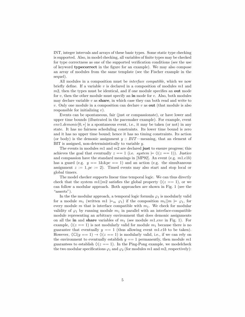
INT, integer intervals and arrays of these basic types. Some static type checkingis supported. Also, in model checking, all variables of finite types may be checkedfor type correctness as one of the supported verification conditions (see the useof keyword typecorrect in the figure for an example). We may also composean array of modules from the same template (see the Fischer example in thesequel).

All modules in a composition must be interface compatible, which we nowbriefly define. If a variable v is declared in a composition of modules m1 andm2, then the types must be identical, and if one module specifies an out modefor v, then the other module must specify an in mode for v. Also, both modulesmay declare variable v as share, in which case they can both read and write tov. Only one module in a composition can declare v as out (that module is alsoresponsible for initializing v).

Events can be spontaneous, fair (just or compassionate), or have lower andupper time bounds (illustrated in the pacemaker example). For example, eventenv1.demonic[0, ∗] is a spontaneous event, i.e., it may be taken (or not) in anystate. It has no fairness scheduling constraints. Its lower time bound is zeroand it has no upper time bound; hence it has no timing constraints. Its action(or body) is the demonic assignment y :: BIT—meaning, that an element ofBIT is assigned, non-deterministically to variable y.

The events in modules m1 and m2 are declared just to ensure progress; thisachieves the goal that eventually z == 1 (i.e. system |= ♦(z == 1)). Justiceand compassion have the standard meanings in [MP92]. An event (e.g. m1.e1b)has a guard (e.g. y == 1&&pc == 1) and an action (e.g. the simultaneousassignment z := 1, pc := 2). Timed events may also start and stop local orglobal timers.

The model checker supports linear time temporal logic. We can thus directlycheck that the system m1||m2 satisfies the global property ♦(z == 1), or wecan follow a modular approach. Both approaches are shown in Fig. 1 (see the“asserts”).

In the the modular approach, a temporal logic formula ϕ1 is modularly validfor a module m1 (written m1 |=m ϕ1) if the composition m1||m |= ϕ1, forevery module m that is interface compatible with m1. We check for modularvalidity of ϕ1 by running module m1 in parallel with an interface-compatiblemodule representing an arbitrary environment that does demonic assignmentson all the in and share variables of m1 (see module m1 env in Fig. 1). Forexample, ♦(z == 1) is not modularly valid for module m1 because there is noguarantee that eventually y == 1 (thus allowing event m1.e1b to be taken).However, ♦�(y == 1) → ♦(z == 1) is modularly valid, i.e., if we can rely onthe environment to eventually establish y == 1 permanently, then module m1guarantees to establish ♦(z == 1). In the Ping-Pong example, we modelcheckthe two modular specifications ϕ1 and ϕ2 (for modulesm1 andm2, respectively):

5

inv: x ≤ maxwait

ready

inv: x ≤ maxwait

ready

vsense![x ≥ minwait]/x := 0

vpace?[true]/x := 0

(a) Model of Heart

inv: x ≤ riwaitRI

inv: x ≤ riwaitRI

inv: x ≤ V RPwaitVRP

inv: x ≤ V RPwaitVRP

vpace![x ≥ ri]/x := 0, ri := LRI, hp := false

vsense?[true]/x := 0, ri := HRI, hp := true

[x ≥ V RP ]/hpenable := hp, started := true

(b) Model of Ventricle Controller

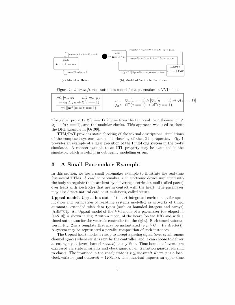
Figure 2: Uppaal/timed-automata model for a pacemaker in VVI mode

m1 |=m ϕ1 m2 |=m ϕ2

|= ϕ1 ∧ ϕ2 → ♦(z == 1)

m1||m2 |= ♦(z == 1)

ϕ1 : ♦�(x == 1) ∧ [♦�(y == 1)→ ♦(z == 1)]ϕ2 : ♦�(x == 1)→ ♦�(y == 1)

The global property ♦(z == 1) follows from the temporal logic theorem ϕ1 ∧ϕ2 → ♦(z == 1), and the modular checks. This approach was used to checkthe DRT example in [Ost99].

TTM/PAT provides static checking of the textual descriptions, simulationsof the composed systems, and modelchecking of the LTL properties. Fig. 1provides an example of a legal execution of the Ping-Pong system in the tool’ssimulator. A counter-example to an LTL property may be examined in thesimulator, which is helpful in debugging modelling errors.

3 A Small Pacemaker Example

In this section, we use a small pacemaker example to illustrate the real-timefeatures of TTMs. A cardiac pacemaker is an electronic device implanted intothe body to regulate the heart beat by delivering electrical stimuli (called paces)over leads with electrodes that are in contact with the heart. The pacemakermay also detect natural cardiac stimulations, called senses.

Uppaal model. Uppaal is a state-of-the-art integrated environment for spec-ification and verification of real-time systems modelled as networks of timedautomata, extended with data types (such as bounded integers and arrays)[ABB+01]. An Uppaal model of the VVI mode of a pacemaker (developed in[JLS10]) is shown in Fig. 2 with a model of the heart (on the left) and with atimed automaton for the ventricle controller (on the right). Each timed automa-ton in Fig. 2 is a template that may be instantiated (e.g. V C = V entricle()).A system may be represented a parallel composition of such instances.

The Uppaal heart model is ready to accept a pacing signal (over synchronouschannel vpace) whenever it is sent by the controller, and it can choose to delivera sensing signal (over channel vsense) at any time. Time bounds of events areexpressed via state invariants and clock guards, i.e., transition guards referringto clocks. The invariant in the ready state is x ≤ maxwait where x is a localclock variable (and maxwait = 1200ms). The invariant imposes an upper time

6

bound by which some transition out of the state must be taken. The guardx ≥ minwait (where minwait = 200ms) imposes a lower time bound on whena sense event is generated.

A pacemaker in the VVI mode operates in a timing cycle that begins witha paced or sensed ventricular event. The basis of the timing cycle is the lowerrate interval (LRI=1000ms), which is the maximum amount of time betweentwo consecutive events in the ventricle. If the LRI elapses and no sensed eventoccurred since the beginning of the cycle, a pace is delivered and the cycle isreset. On the other hand, if a heart beat is sensed, the cycle is reset withoutdelivering a pace.

At the beginning of each cycle, there is a ventricular refractory period(VRP=400ms): chaotic electrical activity in the heart immediately followinga heart beat that may lead to spurious detection of sensed events and can thusinterfere with future pacing. For this reason, sensing is disabled during the VRPperiod. Once the VRP period is over, a sensed ventricular event inhibits thepacing and resets the LRI, starting the new timing cycle.

Hysteresis pacing can be enabled in the VVI mode, when the pacemakerwill delay pacing beyond the LRI to give the heart a chance of resuming normaloperation. In that case, the timing cycle is set to a larger value, namely thehysteresis rate interval (HRI=1200ms). It becomes enabled after a natural heartbeat has been sensed. In [JLS10], hysteresis pacing is applied after a ventricularsense is received, and disabled after a pacing signal is sent.

The ventricle controller has two states: waitRI and waitV RP . The con-troller starts from waitRI and waits for a ventricular sensing or pacing event.If sensing does not occur before the ri (rate interval) period ends, the ventriclecontroller sends a pacing signal to the heart, resets clock x to zero, resets rito LRI, and sets hp (hysteresis pulsing flag) to false, indicating that hysteresispacing is not used in this case. On the other hand, if a ventricular sense eventoccurs before the current LRI cycle ends, ri is reset to HRI instead, allowing alonger period to elapse before pacing. In state waitV RP , the controller waitsfor a VRP period to elapse. It returns to the waitRI state after a VRP pe-riod. Other auxiliary controller variables hpenable and started are used in thespecification.

The requirements are that the heart must pace somewhere between VRPand either LRI or HRI (depending on whether hysteresis pacing is off or on).We could translate the Uppaal model into a corresponding TTM. Instead, wepresent below a more realistic model than the Uppaal version in Fig. 2. We havedeveloped an even more realistic model that separates monitored and controlledvariables properly, and considers electrical noise that could be confused withheart beats during the refactory period. Space considerations prevent us frompresenting it.

Issues in the Uppaal model. The heart in the Uppaal model in Fig. 2 istightly coupled with the controller via synchronous channels. A simulation ofthe Uppaal model thus shows that the heart acting on its own deadlocks immedi-ately due to this tight coupling. It is also unrealistic for the computer controller

7

to respond precisely in sync with a sensing event. In the TTM model, we thusdecouple the heart from the computer controller so that there are states inter-vening between the heart generating a sense signal and the computer respondingto that signal (this could also be done in Uppaal). The TTM heart model canthus beat naturally (or not at all) and may also be paced (if a pace signal isreceived from the computer controller). The heart can thus be simulated onits own in the absence of a controller. It is possible for bad things to happen,non-deterministically, such as missing a beat (or not beating at all). This isdone via the use of a spontaneous event, i.e., an event that has no upper timebound (i.e. deadline) and no fairness assumptions (i.e. justice or compassion).For example, see the natural heart beat event hbn[VRP, ∗] below.

Also, in the Uppaal model, the requirements are written in terms of thephenomena of the computer controller, not in terms of the phenomena of theheart. For example the Uppaal property A�(¬V C.hpenable → V C.x ≤ LRI)states that the heart beats within LRI ticks of the clock in non-hysteresis pacing.That is, whenever the controller auxiliary variable V C.hpeanble holds, then thecomputer clock must be at most LRI. Uppaal properties are written in asubset of branching time logic CTL (called TCTL). The sub-formulas can referto states but not to the occurrence of events. On the other hand, in TTMs,the requirements will be written directly in terms of natural or paced eventsin the heart (in linear time temporal logic LTL). In Uppaal, lower (and upper)time bounds are written as clock guards (and invariants on states). Whereas,in TTMs, events are directly annotated with lower and upper time bounds (andthe necessary clocks are implicitly included).

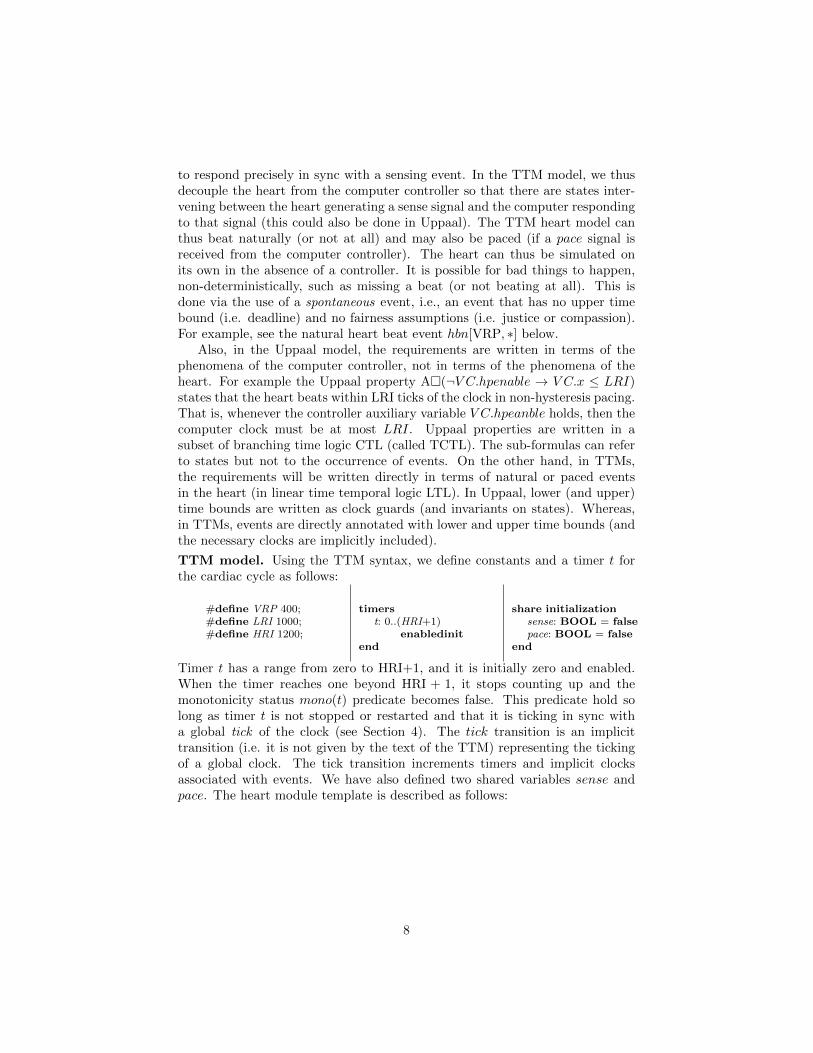
TTM model. Using the TTM syntax, we define constants and a timer t forthe cardiac cycle as follows:

#define VRP 400;#define LRI 1000;#define HRI 1200;

timerst: 0..(HRI+1)

enabledinitend

share initializationsense: BOOL = falsepace: BOOL = false

end

Timer t has a range from zero to HRI+1, and it is initially zero and enabled.When the timer reaches one beyond HRI + 1, it stops counting up and themonotonicity status mono(t) predicate becomes false. This predicate hold solong as timer t is not stopped or restarted and that it is ticking in sync witha global tick of the clock (see Section 4). The tick transition is an implicittransition (i.e. it is not given by the text of the TTM) representing the tickingof a global clock. The tick transition increments timers and implicit clocksassociated with events. We have also defined two shared variables sense andpace. The heart module template is described as follows:

8

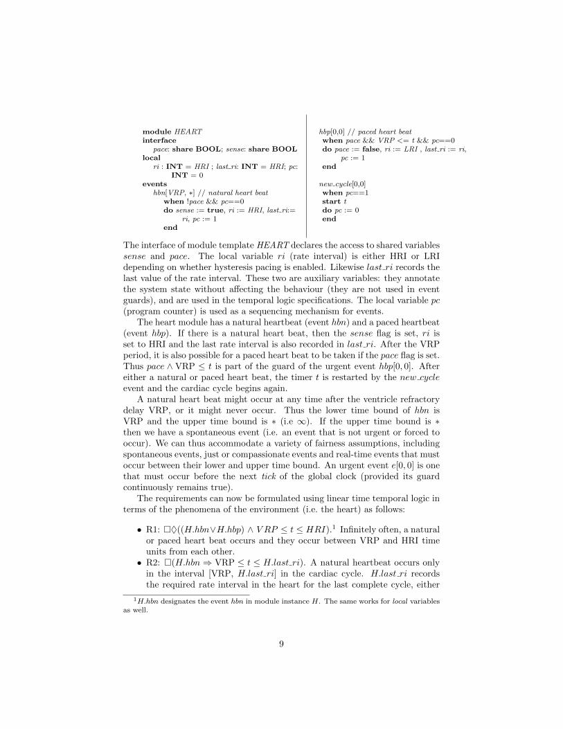
module HEARTinterface

pace: share BOOL; sense: share BOOLlocal

ri : INT = HRI ; last ri: INT = HRI; pc:INT = 0

eventshbn[VRP, ∗] // natural heart beat

when !pace && pc==0do sense := true, ri := HRI, last ri:=

ri, pc := 1end

hbp[0,0] // paced heart beatwhen pace && VRP <= t && pc==0do pace := false, ri := LRI , last ri := ri,

pc := 1end

new cycle[0,0]when pc==1start tdo pc := 0end

The interface of module template HEART declares the access to shared variablessense and pace. The local variable ri (rate interval) is either HRI or LRIdepending on whether hysteresis pacing is enabled. Likewise last ri records thelast value of the rate interval. These two are auxiliary variables: they annotatethe system state without affecting the behaviour (they are not used in eventguards), and are used in the temporal logic specifications. The local variable pc(program counter) is used as a sequencing mechanism for events.

The heart module has a natural heartbeat (event hbn) and a paced heartbeat(event hbp). If there is a natural heart beat, then the sense flag is set, ri isset to HRI and the last rate interval is also recorded in last ri. After the VRPperiod, it is also possible for a paced heart beat to be taken if the pace flag is set.Thus pace ∧ VRP ≤ t is part of the guard of the urgent event hbp[0, 0]. Aftereither a natural or paced heart beat, the timer t is restarted by the new cycleevent and the cardiac cycle begins again.

A natural heart beat might occur at any time after the ventricle refractorydelay VRP, or it might never occur. Thus the lower time bound of hbn isVRP and the upper time bound is ∗ (i.e ∞). If the upper time bound is ∗then we have a spontaneous event (i.e. an event that is not urgent or forced tooccur). We can thus accommodate a variety of fairness assumptions, includingspontaneous events, just or compassionate events and real-time events that mustoccur between their lower and upper time bound. An urgent event e[0, 0] is onethat must occur before the next tick of the global clock (provided its guardcontinuously remains true).

The requirements can now be formulated using linear time temporal logic interms of the phenomena of the environment (i.e. the heart) as follows:

• R1: �♦((H.hbn∨H.hbp) ∧ V RP ≤ t ≤ HRI).1 Infinitely often, a naturalor paced heart beat occurs and they occur between VRP and HRI timeunits from each other.

• R2: �(H.hbn⇒ VRP ≤ t ≤ H.last ri). A natural heartbeat occurs onlyin the interval [VRP, H.last ri] in the cardiac cycle. H.last ri recordsthe required rate interval in the heart for the last complete cycle, either

1H.hbn designates the event hbn in module instance H. The same works for local variablesas well.

9

LRI or HRI, depending on whether hysteresis pacing has been properlyenabled. Thus, �(H.last ri=LRI ∨ H.last ri=HRI) also holds.

• R3: �(H.hbp ⇒ t = H.last ri). A paced heart beat occurs only if thetimer t is at the relevant rate interval.

The ventricle controller will have to estimateH.ri (which, as opposed toH.last ri,relates to the current cycle) in order to ensure that the heart paces accordingto this requirement.

In the Uppaal model there may be a concern that some event (either in theheart module or elsewhere) might illegally set the timer t to a value makingthe specification trivially true. Of course, in a small system, inspection of thetimed automata might re-assure us that all is well. Nevertheless, it would benice to be able to check that timers tick monotonically and uninterruptedlywithout any outside interference. Thus each TTM timer must be equipped witha corresponding monotonicity predicate mono(t) that holds so long as timer t isnot stopped or restarted (see section 4). We may thus check (�♦H.new cycle)∧�(H.new cycle → t = 0) and �(H.new cycle ⇒ mono(t)U((H.hbn ∨H.hbp) ∧(V RP ≤ t ≤ HRI)), which guarantees that there is an appropriate heart beatin each cardiac cycle.

Uppaal does not provide a direct way of checking for zeno behaviour (whichwe must do given that we are using events with upper time bound 0). We cancheck that time always progresses with the LTL formula �♦tick. The tick eventis implicit. That is, it is automatically constructed by the tool with the precisesemantics described in Section 4. The ability to refer to the occurrence of eventsin the TTM assertions makes it possible to specify the required behaviour moredirectly than in Uppaal. The next step is to devise a ventricle controller thatwill satisfy the requirements.

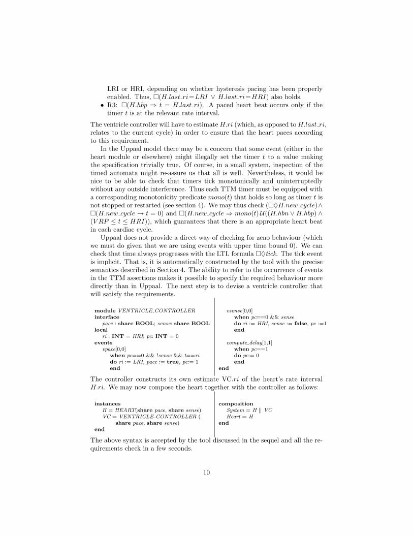
module VENTRICLE CONTROLLERinterface

pace : share BOOL; sense: share BOOLlocal

ri : INT = HRI; pc: INT = 0events

vpace[0,0]when pc==0 && !sense && t==rido ri := LRI, pace := true, pc:= 1end

vsense[0,0]when pc==0 && sensedo ri := HRI, sense := false, pc :=1end

compute delay[1,1]when pc==1do pc:= 0end

end

The controller constructs its own estimate VC.ri of the heart’s rate intervalH.ri. We may now compose the heart together with the controller as follows:

instancesH = HEART(share pace, share sense)VC = VENTRICLE CONTROLLER (

share pace, share sense)end

compositionSystem = H || VCHeart = H

end

The above syntax is accepted by the tool discussed in the sequel and all the re-quirements check in a few seconds.

10

Concrete syntax of event e:

event id [l,u] justwhen grdstart t1, t2stop t3, t4do v1 := exp1,

if condition then v2 := exp2 elseskip fi,

v3 :: 1..4end

Abstract syntax of the event e:

• e.id ∈ ID;• e.l ∈ N;• e.u ∈ N ∪ {∞}• e.fair ∈{spontaneous, just, compassionate}

• e.grd ∈ STATE× TIME→ BOOL;• e.start ⊆ T ;• e.stop ⊆ T ;• e.action ∈ STATE × TIME ↔

STATE;

Figure 3: Concrete and Abstract syntax of TTM events

4 Operational Semantics

Sections 2 and 3 provide some examples of the new concrete textual syntaxfor TTMs. In this section, we provide a one-step operational semantics for acomposition m1||m2|| · · · ||mn of module instances. Following [Ost99] and usingthe mathematical conventions of Event-B [Abr10], let the abstract syntax of aTTM M be given by a 5-tuple, i.e., M = (V, s0, T, t0, E) where 1) V is a setvariable identifiers whether local or declared in a module interface, 2) T is a setof timer identifiers and 3) E is a set of events, 4) s0 ∈ STATE is the TTM’sinitial variable assignment, with STATE , V → VALUE and 5) t0 ∈ TIMEis the TTM’s initial timer assignment, with TIME , T → N. Set E containevents that may change the state. The abstract syntax of each event e ∈ E isspecified by a record as shown on the right of the Fig. 3 (where we use the dotnotation “.” to access the records’ fields).

The event guard grd is any boolean expression in V and T . In the above ex-ample, V = {v1, v2, v3, · · · } and T = {t1, t2, t3, t4, · · · }. The function boundt ∈T → N and type ∈ T → P(N) provide, respectively, the upper bound and typeof each timer. For example, if timer t1 is declared in the TTM as t1 : 0..5, thenboundt(t1) = 5 and type(t1) = {0..6}. As will be detailed below, timers countup to one beyond the specified bound at which point they remain fixed untilthey are restarted.

The event must be taken between its lower time bound l and upper timebound u, provided that its guard remains true. The event action involves si-multaneous assignments to v1, v2, · · · . The notation v3 :: 1..4 is an example of ademonic assignment in which v3 takes any value from 1 to 4. All the assignmentsin the event action are applied simultaneously in one step.

In an assignment y := exp, the expression on the right may use primed(e.g. x′) and unprimed (e.g. x) state variables as well as the initial value oftimers. A variable with a prime refers to the variable’s value in the next stateand a variable without prime refers to its value in the current state. The use ofprimed variables in expressions allows for simpler and more expressive descrip-tions of state changes. The state changes effected by an event e is describedin the abstract syntax by a before-after predicate e.action. The concrete syn-

11

tax also allows for assignments to be embedded in (possibly nested) conditionalstatements.2

In order to build a TTM tool with the PAT framework, we provide a one-stepoperational semantics in labelled transition systems (LTS).

Definition: (Labelled Transition System (LTS)) An LTS is a 4-tuple L =(Π, π0,T,→) where 1) Π is a set of system configurations; 2) π0 ∈ Π is aninitial configuration; 3) T is a set of transitions names; and 4) → ⊆ Π×T×Πis a transition relation.

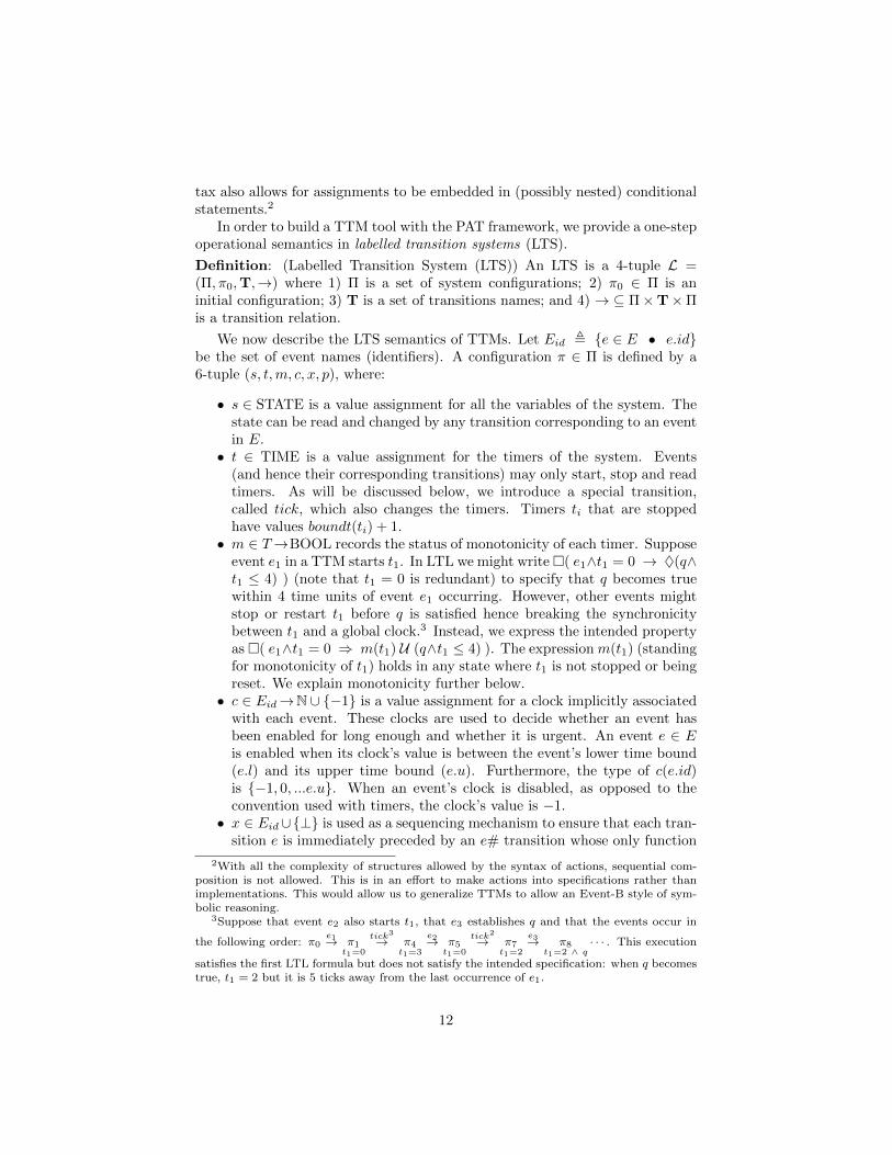
We now describe the LTS semantics of TTMs. Let Eid , {e ∈ E • e.id}be the set of event names (identifiers). A configuration π ∈ Π is defined by a6-tuple (s, t,m, c, x, p), where:

• s ∈ STATE is a value assignment for all the variables of the system. Thestate can be read and changed by any transition corresponding to an eventin E.

• t ∈ TIME is a value assignment for the timers of the system. Events(and hence their corresponding transitions) may only start, stop and readtimers. As will be discussed below, we introduce a special transition,called tick, which also changes the timers. Timers ti that are stoppedhave values boundt(ti) + 1.

• m ∈ T→BOOL records the status of monotonicity of each timer. Supposeevent e1 in a TTM starts t1. In LTL we might write�( e1∧t1 = 0 → ♦(q∧t1 ≤ 4) ) (note that t1 = 0 is redundant) to specify that q becomes truewithin 4 time units of event e1 occurring. However, other events mightstop or restart t1 before q is satisfied hence breaking the synchronicitybetween t1 and a global clock.3 Instead, we express the intended propertyas �( e1∧t1 = 0 ⇒ m(t1) U (q∧t1 ≤ 4) ). The expression m(t1) (standingfor monotonicity of t1) holds in any state where t1 is not stopped or beingreset. We explain monotonicity further below.

• c ∈ Eid→N ∪ {−1} is a value assignment for a clock implicitly associatedwith each event. These clocks are used to decide whether an event hasbeen enabled for long enough and whether it is urgent. An event e ∈ Eis enabled when its clock’s value is between the event’s lower time bound(e.l) and its upper time bound (e.u). Furthermore, the type of c(e.id)is {−1, 0, ...e.u}. When an event’s clock is disabled, as opposed to theconvention used with timers, the clock’s value is −1.

• x ∈ Eid∪{⊥} is used as a sequencing mechanism to ensure that each tran-sition e is immediately preceded by an e# transition whose only function

2With all the complexity of structures allowed by the syntax of actions, sequential com-position is not allowed. This is in an effort to make actions into specifications rather thanimplementations. This would allow us to generalize TTMs to allow an Event-B style of sym-bolic reasoning.

3Suppose that event e2 also starts t1, that e3 establishes q and that the events occur in

the following order: π0e1→ π1

t1=0

tick3

→ π4t1=3

e2→ π5t1=0

tick2

→ π7t1=2

e3→ π8t1=2 ∧ q

· · · . This execution

satisfies the first LTL formula but does not satisfy the intended specification: when q becomestrue, t1 = 2 but it is 5 ticks away from the last occurrence of e1.

12

is to update the monotonicity record m. For example, in the following

execution · · · e1→ π1x=⊥

e2#→ π2x=e2

e2→ π3x=⊥→ · · · , suppose in π1 the value of

timer t2 is 3 and that e2 restarts t2. Then, in π2, we have x = e2 ∧ t2 =3 ∧ m(t2) = false. In π3, we have x = ⊥ ∧ t2 = 0 ∧ m(t2) = true.In order to record the breaking of monotonicity, the e2# transition setsm(t2) to false, which gets set back to true in the following configuration.The precise effect of these transitions will be described below.

• p ∈ Eid ∪ {tick,⊥} holds the name of the last event to be taken ateach configuration. It is ⊥ in the initial configuration as no event hasyet occurred. It allows us to refer to events in LTL formula in order tostate that they have just occurred. For instance, in the formula above,(s, t,m, p) |= e1 ∧ t1 = 0 (which reads: the configuration satisfies theformula) evaluates to p = e1 ∧ t(t1) = 0.

Given a timed transition modelM, the transitions of its corresponding LTSis given as T = Eid ∪ E# ∪ {tick}. As explained above, for each event e ∈E, we introduce a monotonicity breaking transition e.id#. We thus defineE# , {e ∈ E • e.id#}. The tick transition represents one tick of a globalclock. Explicit timers and event lower and upper time bounds are describedwith respect to this tick transition. We define the enabling condition of evente ∈ E as e.en , e.grd ∧ e.l ≤ e.c ≤ e.u, where e.c evaluates to c(e.id)in a configuration whose clock component is c. Thus an event is enabled ina configuration that satisfies its guard and where the event’s implicit clock isbetween its lower and upper time bound.

The initial configuration is defined as π0 = (s0, t0,m0, c0,⊥,⊥), where s0and t0 come from the abstract syntax of the TTM. m0 and c0 are given by:

m0(ti) ≡ t0(ti) = 0

c0(ei.id) =

{0 (s0, t0) |= ei.grd

−1 (s0, t0) 6|= ei.grd

for each ti ∈ T and ei ∈ E. It is implicit in the above formula that m0(ti)depends only on whether or not ti is initially enabled (specified by the key-words enabledinit and disabledinit). If enabledinit, t0(ti) = 0; otherwise,if disabledinit, t0(ti) = boundt(ti) + 1.

An execution σ of the LTS is an infinite sequence, alternating between con-figurations and transitions, written as π0

τ1→ π1τ2→ π2→ · · · where τi ∈ T and

πi ∈ Π.Below, we provide constraints on each one-step relation (π

e→ π′) in anexecution. If an execution σ satisfies all these constraints then we call σ alegal execution. We let ΣL denote the set of all legal executions of the labelledtransition system L. The set ΣL provides a precise and complete definition ofthe behaviour of L.

If a state-formula q holds in a configuration π, then we write π � q. Insome formulas, such as guards, all the components of a configuration are notnecessary. We express this by dropping some components of the configurationon the left of the double turnstile (|=), as in (s0, t0) |= e.grd. Given a temporal

13

logic property ϕ and an LTS L, we write L � ϕ iff ∀σ ∈ ΣL • σ � ϕ. The threepossible transition steps are:

(s, t,m, c,⊥, p) e#→ (s, t,m′, c, e, p) (4.1)

(s, t,m, c, e, p)e→ (s′, t′,m′, c′,⊥, e) (4.2)

(s, t,m, c,⊥, p) tick→ (s, t′,m′, c′,⊥, tick) (4.3)Each of the above transitions have side conditions which we now enumerate.

4.1 Taking e#

The monotonicity breaking transition e#, specified in (4.1), is taken only if(s, t, c) � e.en and the x-component of the configuration is ⊥. For each t ∈ T ,m′(t) ≡ t /∈ e.start ∧ m(t). This ensures that, for timer t, just before it is(re)started, m(t) = false. It is set back to true by the immediately followingevent, e, and it remains true as long as t is not restarted and has not reached itsupper bound. Transition e# modifies only m and x in the configuration, andthus maintains the truth of (s, t, c) � e.en.

4.2 Taking e

The transition e, specified in (4.2), is taken only if (s, t, c) � e.en and the x-component of the configuration is e. The component s′ of the next configurationin an execution is determined nondeterministically by e.action, which is a re-lation rather than a function. This means that any next configuration thatsatisfies the relation can be part of a valid execution, i.e., s′ is only constrainedby (s, t, s′) ∈ e.action. The other components are constrained deterministically.The following function tables specify the updates to m, t and c upon occurrenceof transition e:

For each timer ti ∈ T m′(ti) t′(ti)

ti ∈ e.startti ∈ e.stop impossibleti /∈ e.stop true 0

ti /∈ e.startti ∈ e.stop false boundt(ti) + 1ti /∈ e.stop m(ti) t(ti)

For each event ei ∈ E c′(ei.id)

(s′, t′) 6|= ei.grd -1

(s′, t′) |= ei.grd(s, t) |= ei.grd ∧ ¬ei = e c(ei.id)(s, t) 6|= ei.grd ∨ ei = e 0

In the above, we start and stop the implicit clock of ei as a consequence ofexecuting e, according to whether ei.grd becomes true, is false (i.e. becomes orremains false) or remains true. Since event ei becomes enabled ei.l units afterits guard becomes true, this allows us to know when to consider ei as enabled,

14

i.e., ready to be taken. As a special case, the implicit clock of event e (underconsideration) is restarted when e.grd remains true.

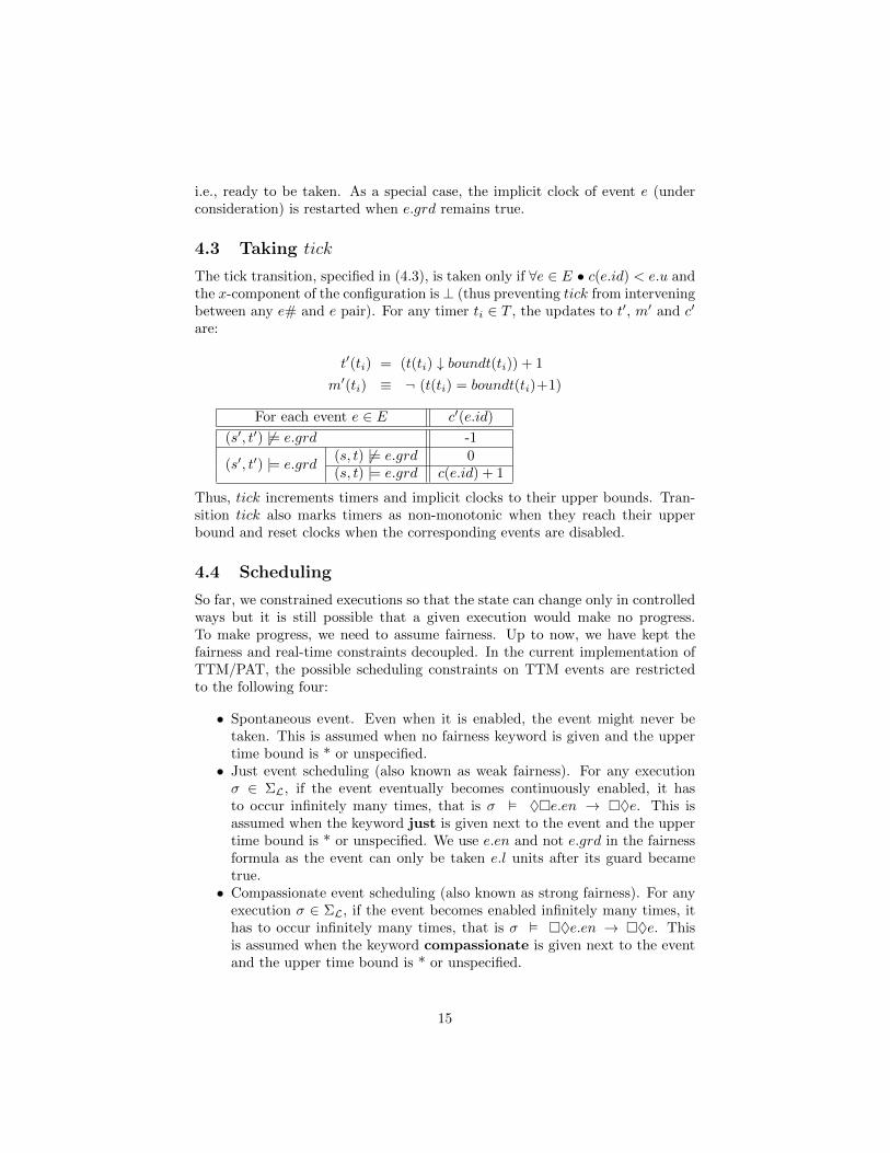
4.3 Taking tick

The tick transition, specified in (4.3), is taken only if ∀e ∈ E • c(e.id) < e.u andthe x-component of the configuration is ⊥ (thus preventing tick from interveningbetween any e# and e pair). For any timer ti ∈ T , the updates to t′, m′ and c′

are:

t′(ti) = (t(ti) ↓ boundt(ti)) + 1

m′(ti) ≡ ¬ (t(ti) = boundt(ti)+1)

For each event e ∈ E c′(e.id)

(s′, t′) 6|= e.grd -1

(s′, t′) |= e.grd(s, t) 6|= e.grd 0(s, t) |= e.grd c(e.id) + 1

Thus, tick increments timers and implicit clocks to their upper bounds. Tran-sition tick also marks timers as non-monotonic when they reach their upperbound and reset clocks when the corresponding events are disabled.

4.4 Scheduling

So far, we constrained executions so that the state can change only in controlledways but it is still possible that a given execution would make no progress.To make progress, we need to assume fairness. Up to now, we have kept thefairness and real-time constraints decoupled. In the current implementation ofTTM/PAT, the possible scheduling constraints on TTM events are restrictedto the following four:

• Spontaneous event. Even when it is enabled, the event might never betaken. This is assumed when no fairness keyword is given and the uppertime bound is * or unspecified.

• Just event scheduling (also known as weak fairness). For any executionσ ∈ ΣL, if the event eventually becomes continuously enabled, it hasto occur infinitely many times, that is σ � ♦�e.en → �♦e. This isassumed when the keyword just is given next to the event and the uppertime bound is * or unspecified. We use e.en and not e.grd in the fairnessformula as the event can only be taken e.l units after its guard becametrue.

• Compassionate event scheduling (also known as strong fairness). For anyexecution σ ∈ ΣL, if the event becomes enabled infinitely many times, ithas to occur infinitely many times, that is σ � �♦e.en → �♦e. Thisis assumed when the keyword compassionate is given next to the eventand the upper time bound is * or unspecified.

15

• Real-time event scheduling. The (finite) upper time bound (u) of the evente is taken as a deadline: if the event’s guard is true for u units of time, ithas to occur within u units of after the guard becomes true or after thelast occurrence of e. To achieve this effect, the event e is treated as just.Since tick won’t occur as long as e is urgent (i.e. e.c = e.u), transition ewill be forced to occur (unless some other event occurs and disables it).

To accurately model time, the tick transition is treated as compassionatein the LTS. This ensures that time progresses except in cases of zeno-behaviors(discussed below).

Spontaneous events cannot be used to establish liveness properties. Justiceand compassion are strong enough assumptions to establish liveness propertiesbut not real-time properties. Finally, real-time events can establish both livenessand real-time properties.

The above semantics allows for zeno behaviours, i.e., it is possible to haveexecutions in which the tick transition does not occur infinitely often (at somepoint, time stops). Zeno behaviour occurs only where there are loops involvingevents with zero upper time bound (i.e. e[0,0]). We could ban e[0,0] eventsaltogether, but that would eliminate behaviours that are feasible and useful,e.g., where we describe a finite sequence of immediately urgent events (not in aloop). We can check that the system is non-zeno by checking that the systemsatisfies �♦tick.

The abstract TTM semantics provided above can be implemented efficiently.For example, in the abstract semantics every event e is preceded by a breakerof monotonicity e#. Most of the e# events do not change the configurationmonotonicity component m and can thus be safely omitted from the reachabilitygraph thereby shrinking it.

5 Performance

We have implemented the TTM textual language and semantics as a plug-inof the PAT toolset. In this section we report on two performance experimentson the plug-in. All experiments were conducted on a 64-bit Windows 7 PCwith Intel(R) Core(TM) i7 CPU 860 @ 2.80 GHz (16.0 GB RAM). The tool(and experimental data) may be downloaded at https://wiki.cse.yorku.ca/project/ttm/.

In section 5.1, we use the DRT (delayed trip reactor) nuclear shutdown ex-ample for the performance comparison. In [LPZ06], the DRT was manuallyencoded and checked in the Uppaal and SAL model-checkers. In that exper-iment, Uppaal performed better than SAL. We compare the performance ofthe TTM/PAT plug-in with these manual encodings and find that TTM/PATperforms significantly better. As reported in [LPZ06], the need to manuallyencode the TTM was a time consuming task. Thus the TTM plug-in has twoadvantages. The TTM encoding to the modelchecker is done automatically andits performance is significantly better.

16

Assertion TCTL of Uppaal LTL of TTM/PAT

Invariantly p S |= A� p S |= � pEventually p S |= A♦ p S |= ♦ pWhenever p, eventually q S |= p −→ q S |= � (p⇒ (♦ q))Infinitely often p S |= true −→ p S |= �♦ pReferring to transition state M.state pc = stateNon-zenoness × S |= �♦ tickp until q, assuming eventually q × S |= p U qp until q × S |= q R pNesting of temporal operators × e.g., � (♦ p⇒ (pUq))Referring to occurrences of event e × eTimer t has increased monotonically × mono (t)Eventually henceforth p × S |= ♦� pS possibly maintains p S |= E� p inverse of S |= ♦ (¬p)S possibly reaches p S |= E♦ p S reaches pNesting of path quantifiers × ×∀♦ ∀� p × ×

Table 1: TTM vs. Uppaal: Language of Assertions

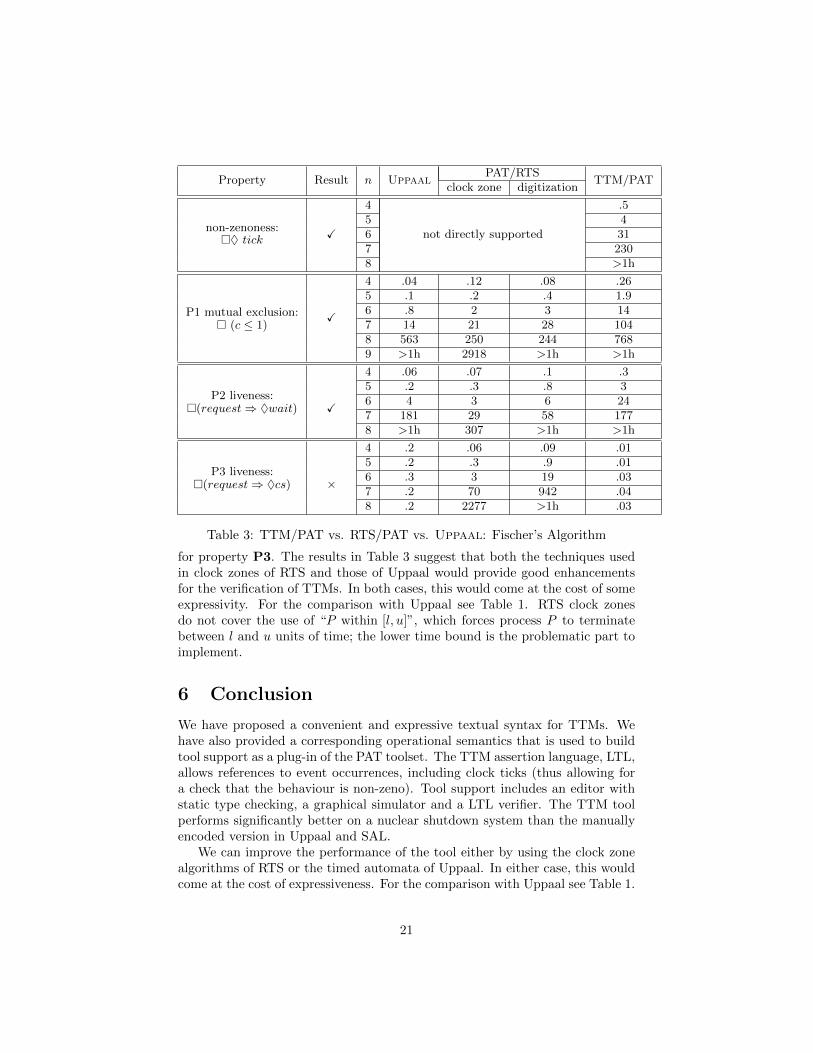
We also use Fischer’s mutual exclusion algorithm to compare the native veri-fication performance of the TTM/PAT plug-in versus Uppaal and the RTS/PATplug-in (see Section 5.2 and Table 3). The RTS plug-in has an explicit clock dig-itization mode and an efficient clock zone mode. The performance of the TTMplug-in is within a linear factor of the RTS digital mode. However, as expected,the Uppaal and RTS clock zone mode performed significantly better than theTTM plug-in. We are currently examining how to extend the TTM plug-inwith these more efficient modes. In each case, the extra performance comes atsome expressive cost. For example, in TTMs we have just and fair events notsupported by Uppaal. Uppaal’s subset of the CTL specification language is lessexpressive than the LTL supported by TTMs.

Table 1 shows that Uppaal’s TCTL specification language is less expressivethan that of TTM/PAT. There are temporal properties such as ♦�p that can bespecified and verified in the TTM plug-in but not in Uppaal. Also, non-zenonessand timer monotinicty can be checked directly in the specification language.

5.1 Delayed Reactor Trip System

The DRT (delayed trip reactor) shutdown system is illustrated in Fig. 4. The oldimplementation of the DRT used timers, comparators and logic gates as shownin the figure. The new DRT system is to be implemented on a microprocessorsystem with a cycle time of 100ms. The system samples the inputs and passesthrough a block of control code every 0.1 seconds. A high-level state/eventdescription (SPEC ) of the code that replaces the analogue system is shown tothe right of Fig. 4 ([LPZ06]). When the reactor pressure and power exceedacceptable safety limits in a specified way, we want the DRT control system to

17

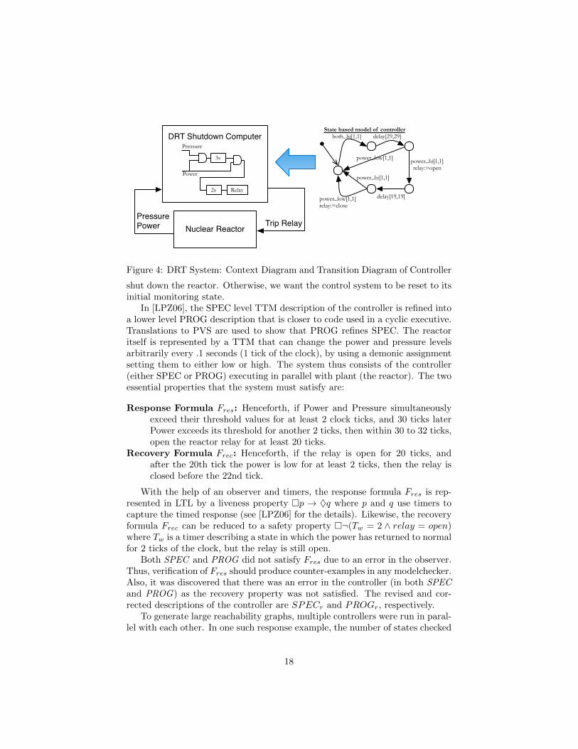
Nuclear ReactorPressurePower Trip Relay

3s

2s Relay

Pressure

Power

DRT Shutdown Computer both_hi[1,1] delay[29,29]

power_low[1,1] power_hi[1,1]relay:=open

delay[19,19]

power_hi[1,1]

power_low[1,1]relay:=close

State based model of controller

Figure 4: DRT System: Context Diagram and Transition Diagram of Controller

shut down the reactor. Otherwise, we want the control system to be reset to itsinitial monitoring state.

In [LPZ06], the SPEC level TTM description of the controller is refined intoa lower level PROG description that is closer to code used in a cyclic executive.Translations to PVS are used to show that PROG refines SPEC. The reactoritself is represented by a TTM that can change the power and pressure levelsarbitrarily every .1 seconds (1 tick of the clock), by using a demonic assignmentsetting them to either low or high. The system thus consists of the controller(either SPEC or PROG) executing in parallel with plant (the reactor). The twoessential properties that the system must satisfy are:

Response Formula Fres: Henceforth, if Power and Pressure simultaneouslyexceed their threshold values for at least 2 clock ticks, and 30 ticks laterPower exceeds its threshold for another 2 ticks, then within 30 to 32 ticks,open the reactor relay for at least 20 ticks.

Recovery Formula Frec: Henceforth, if the relay is open for 20 ticks, andafter the 20th tick the power is low for at least 2 ticks, then the relay isclosed before the 22nd tick.

With the help of an observer and timers, the response formula Fres is rep-resented in LTL by a liveness property �p → ♦q where p and q use timers tocapture the timed response (see [LPZ06] for the details). Likewise, the recoveryformula Frec can be reduced to a safety property �¬(Tw = 2 ∧ relay = open)where Tw is a timer describing a state in which the power has returned to normalfor 2 ticks of the clock, but the relay is still open.

Both SPEC and PROG did not satisfy Fres due to an error in the observer.Thus, verification of Fres should produce counter-examples in any modelchecker.Also, it was discovered that there was an error in the controller (in both SPECand PROG) as the recovery property was not satisfied. The revised and cor-rected descriptions of the controller are SPECr and PROGr, respectively.

To generate large reachability graphs, multiple controllers were run in paral-lel with each other. In one such response example, the number of states checked

18

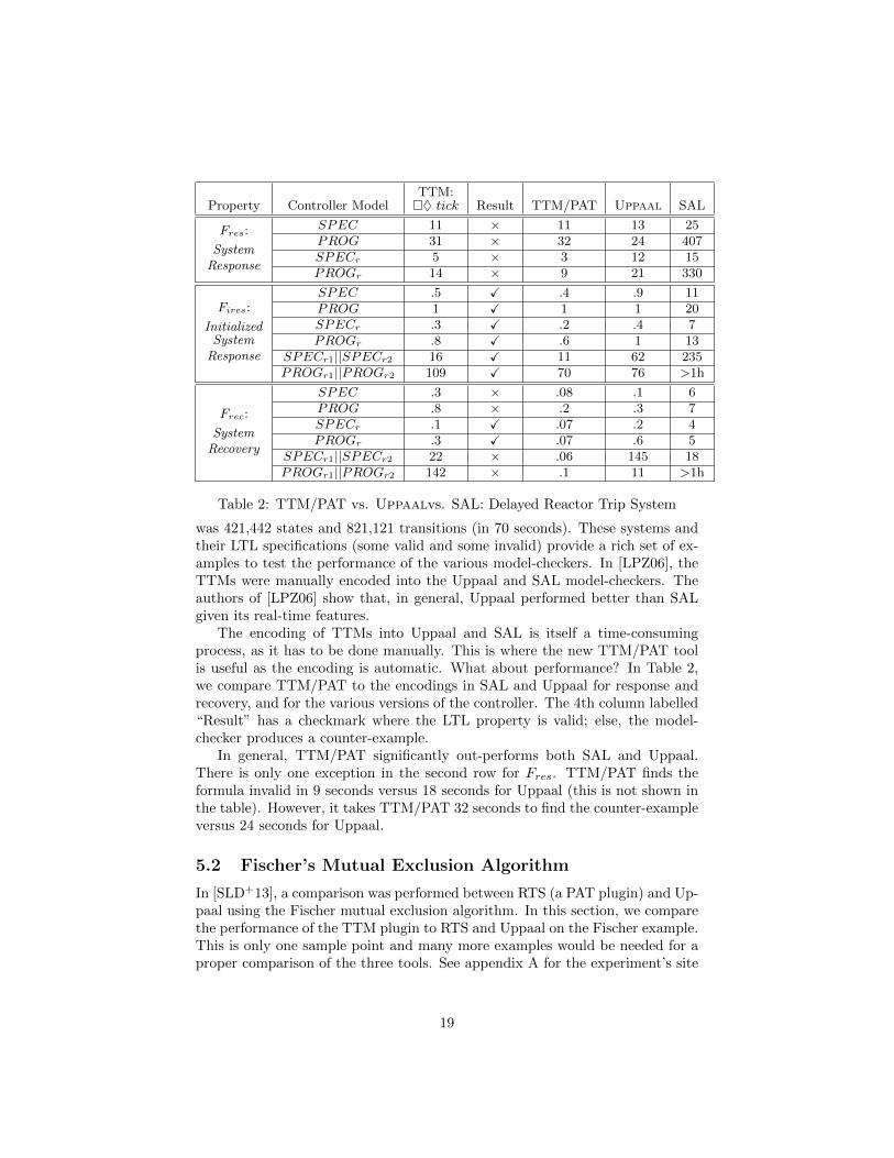
Property Controller ModelTTM:�♦ tick Result TTM/PAT Uppaal SAL

Fres:

SystemResponse

SPEC 11 × 11 13 25PROG 31 × 32 24 407SPECr 5 × 3 12 15PROGr 14 × 9 21 330

Fires:

InitializedSystemResponse

SPEC .5 X .4 .9 11PROG 1 X 1 1 20SPECr .3 X .2 .4 7PROGr .8 X .6 1 13

SPECr1||SPECr2 16 X 11 62 235PROGr1||PROGr2 109 X 70 76 >1h

Frec:

SystemRecovery

SPEC .3 × .08 .1 6PROG .8 × .2 .3 7SPECr .1 X .07 .2 4PROGr .3 X .07 .6 5

SPECr1||SPECr2 22 × .06 145 18PROGr1||PROGr2 142 × .1 11 >1h

Table 2: TTM/PAT vs. Uppaalvs. SAL: Delayed Reactor Trip System

was 421,442 states and 821,121 transitions (in 70 seconds). These systems andtheir LTL specifications (some valid and some invalid) provide a rich set of ex-amples to test the performance of the various model-checkers. In [LPZ06], theTTMs were manually encoded into the Uppaal and SAL model-checkers. Theauthors of [LPZ06] show that, in general, Uppaal performed better than SALgiven its real-time features.

The encoding of TTMs into Uppaal and SAL is itself a time-consumingprocess, as it has to be done manually. This is where the new TTM/PAT toolis useful as the encoding is automatic. What about performance? In Table 2,we compare TTM/PAT to the encodings in SAL and Uppaal for response andrecovery, and for the various versions of the controller. The 4th column labelled“Result” has a checkmark where the LTL property is valid; else, the model-checker produces a counter-example.

In general, TTM/PAT significantly out-performs both SAL and Uppaal.There is only one exception in the second row for Fres. TTM/PAT finds theformula invalid in 9 seconds versus 18 seconds for Uppaal (this is not shown inthe table). However, it takes TTM/PAT 32 seconds to find the counter-exampleversus 24 seconds for Uppaal.

5.2 Fischer’s Mutual Exclusion Algorithm

In [SLD+13], a comparison was performed between RTS (a PAT plugin) and Up-paal using the Fischer mutual exclusion algorithm. In this section, we comparethe performance of the TTM plugin to RTS and Uppaal on the Fischer example.This is only one sample point and many more examples would be needed for aproper comparison of the three tools. See appendix A for the experiment’s site

19

where the Uppaal and RTS details are made available.The PAT toolset provides both digitization (using BDDs) and more efficient

symbolic clock zone algorithms (using difference bound matrices) for checkingRTS models. The TTM plugin uses the explicit state algorithms of the toolset.We thus expect that the TTM performance will be similar to digitization butslower than clock zones. To obtain better performance, we have the choice ofeither using Uppaal or the difference bound matrix techniques. The experimentin this section was performed to help us with that choice.

We build the TTM model (see Appendix A) to be as close as possible to theRTS model at the experiment’s site. The system under verification consists ofn copies of processes running in parallel, using the indexed parallel compositionsyntax:

composition fischer = || i: 1..n @ PROCESS(share x, share c, in i) end

All processes, each identified by an integer i, share two global variables: mutexx and counter c. The mutex may hold the identifier of any process or −1 todenote system idleness. The counter records the number of processes that haveentered their critical section. Process instances execute as follows: 1) await thesystem being idle; 2) signal that it intends to enter its critical section (CS) byupdating x to its identifier i within δ ticks of the clock; 3) delay for exactly εticks of the clock. 1,2 and 3 are repeated as long as the process gets overtaken.4) enter its CS, incrementing counter c; and 5) exit from its its CS, decrementingcounter c, if applicable. We name the state between 2) and 3) request, thatbetween 3) and 4) wait and that between 4) and 5) cs. The following propertiesare commonly relevant for mutual exclusion algorithms.

P1: Mutual Exclusion. At most one process is in its CS at any time: � (c ≤1).

P2: Liveness A process successfully signalling its intent of entering the CSwill get to wait in the appropriate state for access: �(request→ ♦wait).

P3: Starvation freedom A process successfully signalling its intent of enter-ing the CS eventually does enter its CS: �(request→ ♦cs).

When checking liveness properties in RTS, we can specify whether to check:all, event level weak and strong fairness, process level weak and strong fairnessand global fairness. Only global fairness (a very strong assumption) successfullyestablished the starvation freedom property. The same situation applies to theTTM model. Uppaal does not have the facilities to check properties under anyfairness assumptions. TTMs provide the option to choose fairness on an eventby event basis. In Table 3, we compare the performance of the three toolswithout any fairness assumptions. TTM/PAT also provides the ability to checkfor non-zeno behavior, a facility not provided by the other tools. Results forthis property are also reported by the table.

Our experiment shows that, in determining that properties P1 and P2 arevalid, the clock zone mode of RTS is faster than Uppaal (see Table 3). Thespeed of TTM/PAT is within a factor between 3 and 4 of the digitization modeof RTS. TTM/PAT is almost as fast as Uppaal in producing counter examples

20

Property Result n UppaalPAT/RTS

TTM/PATclock zone digitization

non-zenoness:�♦ tick X

4

not directly supported

.55 46 317 2308 >1h

P1 mutual exclusion:� (c ≤ 1)

X

4 .04 .12 .08 .265 .1 .2 .4 1.96 .8 2 3 147 14 21 28 1048 563 250 244 7689 >1h 2918 >1h >1h

P2 liveness:�(request⇒ ♦wait) X

4 .06 .07 .1 .35 .2 .3 .8 36 4 3 6 247 181 29 58 1778 >1h 307 >1h >1h

P3 liveness:�(request⇒ ♦cs) ×

4 .2 .06 .09 .015 .2 .3 .9 .016 .3 3 19 .037 .2 70 942 .048 .2 2277 >1h .03

Table 3: TTM/PAT vs. RTS/PAT vs. Uppaal: Fischer’s Algorithm

for property P3. The results in Table 3 suggest that both the techniques usedin clock zones of RTS and those of Uppaal would provide good enhancementsfor the verification of TTMs. In both cases, this would come at the cost of someexpressivity. For the comparison with Uppaal see Table 1. RTS clock zonesdo not cover the use of “P within [l, u]”, which forces process P to terminatebetween l and u units of time; the lower time bound is the problematic part toimplement.

6 Conclusion

We have proposed a convenient and expressive textual syntax for TTMs. Wehave also provided a corresponding operational semantics that is used to buildtool support as a plug-in of the PAT toolset. The TTM assertion language, LTL,allows references to event occurrences, including clock ticks (thus allowing fora check that the behaviour is non-zeno). Tool support includes an editor withstatic type checking, a graphical simulator and a LTL verifier. The TTM toolperforms significantly better on a nuclear shutdown system than the manuallyencoded version in Uppaal and SAL.

We can improve the performance of the tool either by using the clock zonealgorithms of RTS or the timed automata of Uppaal. In either case, this wouldcome at the cost of expressiveness. For the comparison with Uppaal see Table 1.

21

In RTS, the construct “P within [l, u]”, which forces process P to terminatebetween l and u units of time, is not supported by the clock zone algorithms;the lower time bound is the problematic part to implement. In future work, weintend to explore the clock zone algorithms of RTS as these are already availablein the PAT toolset.

The TTM/PAT tool already supports an assume-guarantee style of compo-sitional reasoning (see Section 2). The use of linear time temporal logic bettersupports compositional reasoning than branching time logic [Var01]. Eventactions are specified as before-after predicates allowing us to enhance composi-tional reasoning using methods developed in UNITY [CM89].

Acknowledgements: Our sincere thanks to Prof. Yang Liu (School of Com-puter Engineering, Nanyang Technological University) and to Prof. Jun Sun(Singapore University of Technology and Design) for their development of thePAT toolset and for their help in developing the TTM plug-in.

References

[ABB+01] T. Amnell, G. Behrmann, J. Bengtsson, P. R. D’Argenio, A. David,A. Fehnker, T. Hune, B. Jeannet, K. G. Larsen, M. O. Moller, P. Pet-tersson, C. Weise, W. Yi. Uppaal - Now, Next, and Future. InMOVEP. LNCS 2067, pp. 99–124. 2001.

[Abr10] J.-R. Abrial. Modeling in Event-B. Cambridge University Press,2010.

[CM89] K. M. Chandy, J. Misra. Parallel program design - a foundation.Addison-Wesley, 1989.

[JLS10] E. Jee, I. Lee, O. Sokolsky. Assurance Cases in Model-Driven Devel-opment of the Pacemaker Software. In Margaria and Steffen (eds.),ISoLA 2010: Part II. Volume LNCS 6416. 2010.

[LPZ06] M. Lawford, V. Pantelic, H. Zhang. Towards Integrated Verificationof Timed Transition Models. Fundamenta Informaticae 70(1,2):75–110, 2006.

[MP92] Z. Manna, A. Pnueli. The Temporal Logic of ractive and ConcurrentSystems: Specification. Springer–Verlag, 1992.

[Ost99] J. S. Ostroff. Composition and Refinement of Discrete Real-TimeSystems. ACM Transaction on Software Engineering Methodology8(1):1–48, 1999.

[SLD+13] J. Sun, Y. Liu, J. S. Dong, Y. Liu, L. Shi, E. Andre. Modeling andverifying hierarchical real-time systems using stateful timed CSP.ACM Transaction on Software Engineering Methodology 22(1):3:1–3:29, 2013.

[Var01] M. Y. Vardi. Branching vs. Linear Time: Final Showdown. InTACAS 2001. Volume LNCS 2031, Springer-Verlag, pp. 1–22. 2001.

22

// Fischer’s mutual exclusion algorithm

#define idle −1;#define n 9;#define delta 3;#define epsilon 4;

share initializationx: INT = idle //semaphorec: INT = 0

end

module PROCESSinterface

x: share INTc: share INT//no. of processes

//inside critical regioni: in INT

localpc: INT = 0

events

await[0, 0]when pc==0 && x==idledo pc := 1end

update[0, delta]when pc == 1do x := i, pc := 2end

delay[epsilon, epsilon]when pc==2do if(x == i) then pc := 3

else pc := 0fi

end

enterwhen pc==3 && x==ido c++, pc:=4end

exitwhen pc==4do c−−, pc:=0, x:=idleend

end

compositionfischer = ||i:1..n @

PROCESS(share x, share c, in i)end

#define cgreater1 c>1;#define pc1 fischer[0].pc==1;#define pc2 fischer[0].pc==2;#define pc4 fischer[0].pc==4;

#assert fischer |= []!cgreater1;//mutex#assert fischer |= [](pc1 −> <> pc2);#assert fischer |= [](pc1 −> <> pc4);#assert fischer |= []<>tick;

Figure 5: TTM model of the Fischer mutual exclusion algorithm

A Appendix

Fig. 5 provides the TTM model of the Fischer algorithm. The TTM modelcorresponds to the RTS and the Uppaal models provided at the experiment siteat http://www.comp.nus.edu.sg/˜pat/rts/. The urgent await[0, 0] event inFig. 5 matches an equivalent urgent transition in the RTS model. The Uppaalmodel provided at the above site did not make that event urgent. However, weused both the RTS and the Uppaal models as they appear at the experimentalsite.

23