TSSB

(Trading System Synthesis and Boosting)

User’s Manual 1.94

Table of Contents

General Operation . . . . . . . . . . . . . . . . . . . . . . . . . . . . . . . . . . . . . . . . . . . . . . . . . . . . . . . . . . . 1

Files. . . . . . . . . . . . . . . . . . . . . . . . . . . . . . . . . . . . . . . . . . . . . . . . . . . . . . . . . . . . . . . . . . . . . . . 2Market histories . . . . . . . . . . . . . . . . . . . . . . . . . . . . . . . . . . . . . . . . . . . . . . . . . . . . . . . 2

Removing Market Prices with Zero Volume . . . . . . . . . . . . . . . . . . . . . . . . . . . . . . . . 3Market List . . . . . . . . . . . . . . . . . . . . . . . . . . . . . . . . . . . . . . . . . . . . . . . . . . . . . . . . . . . 4Variable List . . . . . . . . . . . . . . . . . . . . . . . . . . . . . . . . . . . . . . . . . . . . . . . . . . . . . . . . . . 4The Script File . . . . . . . . . . . . . . . . . . . . . . . . . . . . . . . . . . . . . . . . . . . . . . . . . . . . . . . . 5

Initialization Commands . . . . . . . . . . . . . . . . . . . . . . . . . . . . . . . . . . . . . . . . . . . . . 5Intraday Trading Commands . . . . . . . . . . . . . . . . . . . . . . . . . . . . . . . . . . . . . . . . . . 7Saving and Restoring the Database . . . . . . . . . . . . . . . . . . . . . . . . . . . . . . . . . . . . . . 8Filtering a Haugen Alpha File . . . . . . . . . . . . . . . . . . . . . . . . . . . . . . . . . . . . . . . . 11Reading an HMB file . . . . . . . . . . . . . . . . . . . . . . . . . . . . . . . . . . . . . . . . . . . . . . 11Statistical Test Commands . . . . . . . . . . . . . . . . . . . . . . . . . . . . . . . . . . . . . . . . . . . 12Model, Committee, and Oracle Commands. . . . . . . . . . . . . . . . . . . . . . . . . . . . . . . . 15Find Groups Command. . . . . . . . . . . . . . . . . . . . . . . . . . . . . . . . . . . . . . . . . . . . . 16Regression Classes . . . . . . . . . . . . . . . . . . . . . . . . . . . . . . . . . . . . . . . . . . . . . . . . . 20Preserving Predicted Values for Trade Simulator . . . . . . . . . . . . . . . . . . . . . . . . . . . 22

Output Files . . . . . . . . . . . . . . . . . . . . . . . . . . . . . . . . . . . . . . . . . . . . . . . . . . . . . . . . . . . . . . . 23AUDIT.LOG . . . . . . . . . . . . . . . . . . . . . . . . . . . . . . . . . . . . . . . . . . . . . . . . . . . . . . . . 23REPORT.LOG . . . . . . . . . . . . . . . . . . . . . . . . . . . . . . . . . . . . . . . . . . . . . . . . . . . . . . 25

Variables . . . . . . . . . . . . . . . . . . . . . . . . . . . . . . . . . . . . . . . . . . . . . . . . . . . . . . . . . . . . . . . . . . 26References to an Index Market . . . . . . . . . . . . . . . . . . . . . . . . . . . . . . . . . . . . . . . . . . 26Historical Normalization . . . . . . . . . . . . . . . . . . . . . . . . . . . . . . . . . . . . . . . . . . . . . . . 27Cross-Market Normalization . . . . . . . . . . . . . . . . . . . . . . . . . . . . . . . . . . . . . . . . . . . . 29Pooled Variables . . . . . . . . . . . . . . . . . . . . . . . . . . . . . . . . . . . . . . . . . . . . . . . . . . . . . . 30Mahalanobis Distance . . . . . . . . . . . . . . . . . . . . . . . . . . . . . . . . . . . . . . . . . . . . . . . . . 31Absorption Ratio . . . . . . . . . . . . . . . . . . . . . . . . . . . . . . . . . . . . . . . . . . . . . . . . . . . . . 32Residuals . . . . . . . . . . . . . . . . . . . . . . . . . . . . . . . . . . . . . . . . . . . . . . . . . . . . . . . . . . . . 34Errors in the Raw Market Data . . . . . . . . . . . . . . . . . . . . . . . . . . . . . . . . . . . . . . . . . . 34Families of Variables . . . . . . . . . . . . . . . . . . . . . . . . . . . . . . . . . . . . . . . . . . . . . . . . . . 35

CLOSE TO CLOSE ATRlength . . . . . . . . . . . . . . . . . . . . . . . . . . . . . . . . . . . 35CLOSE MINUS MOVING AVERAGE HistLength ATRlength . . . . . . . . . 35MA DIFFERENCE ShortLength LongLength Lag . . . . . . . . . . . . . . . . . . . . . 35ABS PRICE CHANGE OSCILLATOR ShortLength Multiplier . . . . . . . . . . 36LINEAR PER ATR HistLength ATRlength . . . . . . . . . . . . . . . . . . . . . . . . . 36QUADRATIC PER ATR HistLength ATRlength. . . . . . . . . . . . . . . . . . . . . 36

CUBIC PER ATR HistLength ATRlength . . . . . . . . . . . . . . . . . . . . . . . . . . . 36RSI HistLength . . . . . . . . . . . . . . . . . . . . . . . . . . . . . . . . . . . . . . . . . . . . . . . . . 37HI_RSI HistLength . . . . . . . . . . . . . . . . . . . . . . . . . . . . . . . . . . . . . . . . . . . . . 37LO_RSI HistLength . . . . . . . . . . . . . . . . . . . . . . . . . . . . . . . . . . . . . . . . . . . . . 37COND_RSI HistLength . . . . . . . . . . . . . . . . . . . . . . . . . . . . . . . . . . . . . . . . . . 37STOCHASTIC K HistLength. . . . . . . . . . . . . . . . . . . . . . . . . . . . . . . . . . . . . . 37STOCHASTIC D HistLength . . . . . . . . . . . . . . . . . . . . . . . . . . . . . . . . . . . . . 37PRICE MOMENTUM HistLength StdDevLength . . . . . . . . . . . . . . . . . . . . . 38LINEAR DEVIATION HistLength . . . . . . . . . . . . . . . . . . . . . . . . . . . . . . . . 38QUADRATIC DEVIATION HistLength. . . . . . . . . . . . . . . . . . . . . . . . . . . . 38CUBIC DEVIATION HistLength . . . . . . . . . . . . . . . . . . . . . . . . . . . . . . . . . . 39DEVIATION FROM INDEX FIT HistLength MovAvgLength . . . . . . . . . . . 39INDEX CORRELATION HistLength . . . . . . . . . . . . . . . . . . . . . . . . . . . . . . 39DELTA INDEX CORRELATION HistLength DeltaLength . . . . . . . . . . . . 39ADX HistLength . . . . . . . . . . . . . . . . . . . . . . . . . . . . . . . . . . . . . . . . . . . . . . . 40MIN ADX HistLength MinLength . . . . . . . . . . . . . . . . . . . . . . . . . . . . . . . . . 40RESIDUAL MIN ADX HistLength MinLength . . . . . . . . . . . . . . . . . . . . . . 40MAX ADX HistLength MaxLength. . . . . . . . . . . . . . . . . . . . . . . . . . . . . . . . 40RESIDUAL MAX ADX HistLength MaxLength . . . . . . . . . . . . . . . . . . . . 40DELTA ADX HistLength DeltaLength . . . . . . . . . . . . . . . . . . . . . . . . . . . . . 41ACCEL ADX HistLength DeltaLength . . . . . . . . . . . . . . . . . . . . . . . . . . . . . 41INTRADAY INTENSITY HistLength . . . . . . . . . . . . . . . . . . . . . . . . . . . . . 41DELTA INTRADAY INTENSITY HistLength DeltaLength. . . . . . . . . . . . 41PRICE VARIANCE RATIO HistLength Multiplier . . . . . . . . . . . . . . . . . . 42MIN PRICE VARIANCE RATIO HistLen Mult Mlen . . . . . . . . . . . . . . . . . 42MAX PRICE VARIANCE RATIO HistLen Mult Mlen. . . . . . . . . . . . . . . . . 42CHANGE VARIANCE RATIO HistLength Multiplier . . . . . . . . . . . . . . . 42MIN CHANGE VARIANCE RATIO HistLen Mult Mlen . . . . . . . . . . . . . . 42ATR RATIO HistLength Multiplier . . . . . . . . . . . . . . . . . . . . . . . . . . . . . . . . 43DELTA PRICE VARIANCE RATIO HistLength Multiplier . . . . . . . . . . . 43DELTA CHANGE VARIANCE RATIO HistLength Multiplier. . . . . . . . 43DELTA ATR RATIO HistLength Multiplier . . . . . . . . . . . . . . . . . . . . . . . . 43BOLLINGER WIDTH HistLength . . . . . . . . . . . . . . . . . . . . . . . . . . . . . . . . 43DELTA BOLLINGER WIDTH HistLength DeltaLength . . . . . . . . . . . . . . 44PRICE SKEWNESS HistLength Multiplier . . . . . . . . . . . . . . . . . . . . . . . . . . 44CHANGE SKEWNESS HistLength Multiplier. . . . . . . . . . . . . . . . . . . . . . . 44PRICE KURTOSIS HistLength Multiplier . . . . . . . . . . . . . . . . . . . . . . . . . . . 44CHANGE KURTOSIS HistLength Multiplier . . . . . . . . . . . . . . . . . . . . . . . . 45DELTA PRICE SKEWNESS HistLength Multiplier DeltaLength . . . . . . . . . . . 45DELTA CHANGE SKEWNESS HistLength Multiplier DeltaLength . . . . . . . 45DELTA PRICE KURTOSIS HistLength Multiplier DeltaLength . . . . . . . . . . . . 45DELTA CHANGE KURTOSIS HistLength Multiplier DeltaLength . . . . . . . . . 45VOLUME MOMENTUM HistLength Multiplier . . . . . . . . . . . . . . . . . . . . . 45DELTA VOLUME MOMENTUM HistLen Multiplier DeltaLen . . . . . . . . 45

PRICE ENTROPY WordLength . . . . . . . . . . . . . . . . . . . . . . . . . . . . . . . . . . . 46VOLUME ENTROPY WordLength . . . . . . . . . . . . . . . . . . . . . . . . . . . . . . . . 46PRICE MUTUAL INFORMATION WordLength . . . . . . . . . . . . . . . . . . . . 46VOLUME MUTUAL INFORMATION WordLength . . . . . . . . . . . . . . . . . 46REAL MORLET Period . . . . . . . . . . . . . . . . . . . . . . . . . . . . . . . . . . . . . . . . . 47REAL DIFF MORLET Period . . . . . . . . . . . . . . . . . . . . . . . . . . . . . . . . . . . . 47REAL PRODUCT MORLET Period . . . . . . . . . . . . . . . . . . . . . . . . . . . . . . . 47IMAG MORLET Period . . . . . . . . . . . . . . . . . . . . . . . . . . . . . . . . . . . . . . . . . 47IMAG DIFF MORLET Period . . . . . . . . . . . . . . . . . . . . . . . . . . . . . . . . . . . . 47IMAG PRODUCT MORLET Period . . . . . . . . . . . . . . . . . . . . . . . . . . . . . . . 47PHASE MORLET Period . . . . . . . . . . . . . . . . . . . . . . . . . . . . . . . . . . . . . . . . 48DAUB MEAN HistLength Level . . . . . . . . . . . . . . . . . . . . . . . . . . . . . . . . . . 48DAUB MIN HistLength Level . . . . . . . . . . . . . . . . . . . . . . . . . . . . . . . . . . . . 48DAUB MAX HistLength Level . . . . . . . . . . . . . . . . . . . . . . . . . . . . . . . . . . . 48DAUB STD HistLength Level . . . . . . . . . . . . . . . . . . . . . . . . . . . . . . . . . . . . 48DAUB ENERGY HistLength Level . . . . . . . . . . . . . . . . . . . . . . . . . . . . . . . 49DAUB NL ENERGY HistLength Level . . . . . . . . . . . . . . . . . . . . . . . . . . . . 49DAUB CURVE HistLength Level . . . . . . . . . . . . . . . . . . . . . . . . . . . . . . . . . 49VOLUME WEIGHTED MA OVER MA HistLength. . . . . . . . . . . . . . . . . 49DIFF VOLUME WEIGHTED MA OVER MA ShortDist LongDist . . . . . 49PRICE VOLUME FIT HistLength. . . . . . . . . . . . . . . . . . . . . . . . . . . . . . . . . 50DIFF PRICE VOLUME FIT ShortDist LongDist . . . . . . . . . . . . . . . . . . . . 50DELTA PRICE VOLUME FIT HistLength DeltaDist . . . . . . . . . . . . . . . . 50REACTIVITY HistLength . . . . . . . . . . . . . . . . . . . . . . . . . . . . . . . . . . . . . . . 50DELTA REACTIVITY HistLength DeltaDist . . . . . . . . . . . . . . . . . . . . . . . 50MIN REACTIVITY HistLength MinMaxDist . . . . . . . . . . . . . . . . . . . . . . . 51MAX REACTIVITY HistLength MinMaxDist . . . . . . . . . . . . . . . . . . . . . . 51ON BALANCE VOLUME HistLength . . . . . . . . . . . . . . . . . . . . . . . . . . . . 51DELTA ON BALANCE VOLUME HistLength DeltaDist . . . . . . . . . . . . 51POSITIVE VOLUME INDICATOR HistLength . . . . . . . . . . . . . . . . . . . . . 51DELTA POSITIVE VOLUME INDICATOR HistLength DeltaDist . . . . . . 52NEGATIVE VOLUME INDICATOR HistLength . . . . . . . . . . . . . . . . . . . . 52DELTA NEGATIVE VOLUME INDICATOR HistLen DeltaDist. . . . . . . 52PRODUCT PRICE VOLUME HistLength . . . . . . . . . . . . . . . . . . . . . . . . . . 52SUM PRICE VOLUME HistLength . . . . . . . . . . . . . . . . . . . . . . . . . . . . . . . 52DELTA PRODUCT PRICE VOLUME HistLength DeltaDist . . . . . . . . . . 53DELTA SUM PRICE VOLUME HistLength DeltaDist . . . . . . . . . . . . . . . 53N DAY HIGH HistLength . . . . . . . . . . . . . . . . . . . . . . . . . . . . . . . . . . . . . . . 53N DAY LOW HistLength . . . . . . . . . . . . . . . . . . . . . . . . . . . . . . . . . . . . . . . . 53N DAY NARROWER HistLength . . . . . . . . . . . . . . . . . . . . . . . . . . . . . . . . . 53N DAY WIDER HistLength . . . . . . . . . . . . . . . . . . . . . . . . . . . . . . . . . . . . . . 53FTI family... BlockSize HalfLength LowPeriod HighPeriod . . . . . . . . . . . . . . . . . 54FTI LOWPASS BlockSize HalfLength Period . . . . . . . . . . . . . . . . . . . . . . . . . 54FTI MINOR LOWPASS BlockSize HalfLength LowPeriod HighPeriod. . . . . . 54

FTI MAJOR LOWPASS BlockSize HalfLength LowPeriod HighPeriod . . . . . . 55FTI FTI BlockSize HalfLength Period . . . . . . . . . . . . . . . . . . . . . . . . . . . . . . . . 55FTI LARGEST FTI BlockSize HalfLength LowPeriod HighPeriod . . . . . . . . . 55FTI MINOR FTI BlockSize HalfLength LowPeriod HighPeriod . . . . . . . . . . . . 55FTI MAJOR FTI BlockSize HalfLength LowPeriod HighPeriod . . . . . . . . . . . . 55FTI LARGEST PERIOD BlockSize HalfLength LowPeriod HighPeriod . . . . . 55FTI MINOR PERIOD BlockSize HalfLength LowPeriod HighPeriod. . . . . . . . 55FTI MAJOR PERIOD BlockSize HalfLength LowPeriod HighPeriod. . . . . . . . 56FTI CRAT BlockSize HalfLength LowPeriod HighPeriod . . . . . . . . . . . . . . . . . 56FTI MINOR BEST CRAT BlockSize HalfLength LowPeriod HighPeriod . . . . 56FTI MAJOR BEST CRAT BlockSize HalfLength LowPeriod HighPeriod . . . . 56FTI BOTH BEST CRAT BlockSize HalfLength LowPeriod HighPeriod . . . . . 56DETRENDED RSI DetrendedLength DetrenderLength Lookback . . . . . . . . . . 56THRESHOLDED RSI LookbackLength UpperThresh LowerThresh . . . . . . . . 57PURIFIED INDEX Norm HistLen Npred Nfam Nlooks Look1 ... . . . . . . . 58AROON UP Lookback . . . . . . . . . . . . . . . . . . . . . . . . . . . . . . . . . . . . . . . . . . . 60AROON DOWN Lookback . . . . . . . . . . . . . . . . . . . . . . . . . . . . . . . . . . . . . . . 60AROON DIFF Lookback . . . . . . . . . . . . . . . . . . . . . . . . . . . . . . . . . . . . . . . . . 60NEW HIGH Lookback . . . . . . . . . . . . . . . . . . . . . . . . . . . . . . . . . . . . . . . . . . . 60NEW LOW Lookback . . . . . . . . . . . . . . . . . . . . . . . . . . . . . . . . . . . . . . . . . . . . 60NEW EXTREME Lookback . . . . . . . . . . . . . . . . . . . . . . . . . . . . . . . . . . . . . . 60OFF HIGH Lookback ATRlookback . . . . . . . . . . . . . . . . . . . . . . . . . . . . . . . 61ABOVE LOW Lookback ATRlookback . . . . . . . . . . . . . . . . . . . . . . . . . . . . . 61ABOVE MA BI Lookback . . . . . . . . . . . . . . . . . . . . . . . . . . . . . . . . . . . . . . . . 61ABOVE MA TRI Lookback . . . . . . . . . . . . . . . . . . . . . . . . . . . . . . . . . . . . . . 61ROC POSITIVE BI Lookback . . . . . . . . . . . . . . . . . . . . . . . . . . . . . . . . . . . . . 61ROC POSITIVE TRI Lookback. . . . . . . . . . . . . . . . . . . . . . . . . . . . . . . . . . . . 61NEWHI Lookback. . . . . . . . . . . . . . . . . . . . . . . . . . . . . . . . . . . . . . . . . . . . . . . 62SUPPORT Lookback . . . . . . . . . . . . . . . . . . . . . . . . . . . . . . . . . . . . . . . . . . . . . 62NEWLO COUNT Lookback . . . . . . . . . . . . . . . . . . . . . . . . . . . . . . . . . . . . . . 62NEWLO Lookback . . . . . . . . . . . . . . . . . . . . . . . . . . . . . . . . . . . . . . . . . . . . . . 63RESISTANCE Lookback . . . . . . . . . . . . . . . . . . . . . . . . . . . . . . . . . . . . . . . . . 63NEWHI COUNT Lookback . . . . . . . . . . . . . . . . . . . . . . . . . . . . . . . . . . . . . . . 63CUBIC FIT VALUE Lookback . . . . . . . . . . . . . . . . . . . . . . . . . . . . . . . . . . . 64CUBIC FIT ERROR Lookback . . . . . . . . . . . . . . . . . . . . . . . . . . . . . . . . . . . . 64DOWN PERSIST . . . . . . . . . . . . . . . . . . . . . . . . . . . . . . . . . . . . . . . . . . . . . . . 65UP PERSIST. . . . . . . . . . . . . . . . . . . . . . . . . . . . . . . . . . . . . . . . . . . . . . . . . . . 65NEXT DAY LOG RATIO . . . . . . . . . . . . . . . . . . . . . . . . . . . . . . . . . . . . . . . 66CLOSE LOG RATIO . . . . . . . . . . . . . . . . . . . . . . . . . . . . . . . . . . . . . . . . . . . 66NEXT DAY ATR RETURN Distance . . . . . . . . . . . . . . . . . . . . . . . . . . . . . . 67CLOSE ATR RETURN Distance . . . . . . . . . . . . . . . . . . . . . . . . . . . . . . . . . . 67OC ATR RETURN Distance . . . . . . . . . . . . . . . . . . . . . . . . . . . . . . . . . . . . . . 68SUBSEQUENT DAY ATR RETURN Lead Distance . . . . . . . . . . . . . . . . . 68NEXT MONTH ATR RETURN Distance . . . . . . . . . . . . . . . . . . . . . . . . . . . 68

INTRADAY RETURN Distance . . . . . . . . . . . . . . . . . . . . . . . . . . . . . . . . . . 68HIT OR MISS Up Down Cutoff ATRdist . . . . . . . . . . . . . . . . . . . . . . . . . . . . 69FUTURE SLOPE Ahead ATRdist . . . . . . . . . . . . . . . . . . . . . . . . . . . . . . . . . 69RSQ FUTURE SLOPE Ahead ATRdist. . . . . . . . . . . . . . . . . . . . . . . . . . . . . 69CURVATURE INDEX LookAhead MinSep SepInc Nseps Vdist . . . . . . . . . 69BULL MinPercentReturn MaxPercentDrawdown MinBars . . . . . . . . . . . . . . . . . 72ENDING BULL MinPctRet MaxPctDD PctThresh MinBars . . . . . . . . . . . . . 73STARTING BULL MinPctRet MaxPctDD PctThresh MinBars . . . . . . . . . . . 74

Examples of Variables . . . . . . . . . . . . . . . . . . . . . . . . . . . . . . . . . . . . . . . . . . . . . . . . . 75

Stationarity Tests . . . . . . . . . . . . . . . . . . . . . . . . . . . . . . . . . . . . . . . . . . . . . . . . . . . . . . . . . . . 76Linear Chi-Square Tests . . . . . . . . . . . . . . . . . . . . . . . . . . . . . . . . . . . . . . . . . . . . . . . . 79

Equal-Spacing Chi-Square . . . . . . . . . . . . . . . . . . . . . . . . . . . . . . . . . . . . . . . . . . 79Equal-Count Chi-Square . . . . . . . . . . . . . . . . . . . . . . . . . . . . . . . . . . . . . . . . . . . 79

Mutual Information With Time . . . . . . . . . . . . . . . . . . . . . . . . . . . . . . . . . . . . . . . . . . 79Boundary T-Tests . . . . . . . . . . . . . . . . . . . . . . . . . . . . . . . . . . . . . . . . . . . . . . . . . . . . . 80

T-Test for Mean . . . . . . . . . . . . . . . . . . . . . . . . . . . . . . . . . . . . . . . . . . . . . . . . . . 80T-Test for Mean Absolute Value . . . . . . . . . . . . . . . . . . . . . . . . . . . . . . . . . . . . . . 80

Boundary U-Tests. . . . . . . . . . . . . . . . . . . . . . . . . . . . . . . . . . . . . . . . . . . . . . . . . . . . . 81U-Test for Mean. . . . . . . . . . . . . . . . . . . . . . . . . . . . . . . . . . . . . . . . . . . . . . . . . . 81U-Test for Mean Absolute Value . . . . . . . . . . . . . . . . . . . . . . . . . . . . . . . . . . . . . . 81U-Test for Deviation from Median . . . . . . . . . . . . . . . . . . . . . . . . . . . . . . . . . . . . . 81

Monthly Tests . . . . . . . . . . . . . . . . . . . . . . . . . . . . . . . . . . . . . . . . . . . . . . . . . . . . . . . . 82Monthly Equal-Spacing Chi-Square . . . . . . . . . . . . . . . . . . . . . . . . . . . . . . . . . . . . 82Monthly Equal-Count Chi-Square . . . . . . . . . . . . . . . . . . . . . . . . . . . . . . . . . . . . . 82Monthly ANOVA for Location . . . . . . . . . . . . . . . . . . . . . . . . . . . . . . . . . . . . . . 82Monthly Kruskal-Wallis for Location . . . . . . . . . . . . . . . . . . . . . . . . . . . . . . . . . . . 82Monthly Kruskal-Wallis for Absolute Location . . . . . . . . . . . . . . . . . . . . . . . . . . . . 83Monthly Kruskal-Wallis for Deviation from Median. . . . . . . . . . . . . . . . . . . . . . . . . 83

Lookahead Analysis . . . . . . . . . . . . . . . . . . . . . . . . . . . . . . . . . . . . . . . . . . . . . . . . . . . . . . . . . 84Specifying Lookahead Analysis Options . . . . . . . . . . . . . . . . . . . . . . . . . . . . . . . . . . . 86An Example of Model Analysis . . . . . . . . . . . . . . . . . . . . . . . . . . . . . . . . . . . . . . . . . . 89An Example of Predictor Analysis. . . . . . . . . . . . . . . . . . . . . . . . . . . . . . . . . . . . . . . . 91

Menu Commands . . . . . . . . . . . . . . . . . . . . . . . . . . . . . . . . . . . . . . . . . . . . . . . . . . . . . . . . . . . 94File Menu Commands . . . . . . . . . . . . . . . . . . . . . . . . . . . . . . . . . . . . . . . . . . . . . . . . . 94

Job Continuation with Multiple Scripts . . . . . . . . . . . . . . . . . . . . . . . . . . . . . . . . . . 95Describe Menu Commands . . . . . . . . . . . . . . . . . . . . . . . . . . . . . . . . . . . . . . . . . . . . . 96

Univariate . . . . . . . . . . . . . . . . . . . . . . . . . . . . . . . . . . . . . . . . . . . . . . . . . . . . . . 96Chi-Square. . . . . . . . . . . . . . . . . . . . . . . . . . . . . . . . . . . . . . . . . . . . . . . . . . . . . . 96Nonredundant Predictor Screening. . . . . . . . . . . . . . . . . . . . . . . . . . . . . . . . . . . . . . 96Market Scan . . . . . . . . . . . . . . . . . . . . . . . . . . . . . . . . . . . . . . . . . . . . . . . . . . . . 96Outlier Scan . . . . . . . . . . . . . . . . . . . . . . . . . . . . . . . . . . . . . . . . . . . . . . . . . . . . . 96

Cross Market AD . . . . . . . . . . . . . . . . . . . . . . . . . . . . . . . . . . . . . . . . . . . . . . . . 97Stationarity . . . . . . . . . . . . . . . . . . . . . . . . . . . . . . . . . . . . . . . . . . . . . . . . . . . . . 98

Plot Menu Commands . . . . . . . . . . . . . . . . . . . . . . . . . . . . . . . . . . . . . . . . . . . . . . . . . 99Series . . . . . . . . . . . . . . . . . . . . . . . . . . . . . . . . . . . . . . . . . . . . . . . . . . . . . . . . . . 99Series + Market . . . . . . . . . . . . . . . . . . . . . . . . . . . . . . . . . . . . . . . . . . . . . . . . . . 99Market . . . . . . . . . . . . . . . . . . . . . . . . . . . . . . . . . . . . . . . . . . . . . . . . . . . . . . . . 99Histogram . . . . . . . . . . . . . . . . . . . . . . . . . . . . . . . . . . . . . . . . . . . . . . . . . . . . . 100Thresholded Histogram . . . . . . . . . . . . . . . . . . . . . . . . . . . . . . . . . . . . . . . . . . . . 101Density Map . . . . . . . . . . . . . . . . . . . . . . . . . . . . . . . . . . . . . . . . . . . . . . . . . . . 102Equity . . . . . . . . . . . . . . . . . . . . . . . . . . . . . . . . . . . . . . . . . . . . . . . . . . . . . . . . 104Prediction Map . . . . . . . . . . . . . . . . . . . . . . . . . . . . . . . . . . . . . . . . . . . . . . . . . . 107Indicator-Target Relationship . . . . . . . . . . . . . . . . . . . . . . . . . . . . . . . . . . . . . . . . 109Lookahead Performance . . . . . . . . . . . . . . . . . . . . . . . . . . . . . . . . . . . . . . . . . . . . 112

Transforms . . . . . . . . . . . . . . . . . . . . . . . . . . . . . . . . . . . . . . . . . . . . . . . . . . . . . . . . . . . . . . . 113The RANDOM Transform . . . . . . . . . . . . . . . . . . . . . . . . . . . . . . . . . . . . . . . . . . . . 113The NOMINAL MAPPING Transform . . . . . . . . . . . . . . . . . . . . . . . . . . . . . . . . . 114The EXPRESSION Transform. . . . . . . . . . . . . . . . . . . . . . . . . . . . . . . . . . . . . . . . . 116

Predefined Variables . . . . . . . . . . . . . . . . . . . . . . . . . . . . . . . . . . . . . . . . . . . . . . 117Basic Operations . . . . . . . . . . . . . . . . . . . . . . . . . . . . . . . . . . . . . . . . . . . . . . . . . 119Vector Operations in Expression Transforms . . . . . . . . . . . . . . . . . . . . . . . . . . . . . 121Logical Evaluation in Expression Transforms . . . . . . . . . . . . . . . . . . . . . . . . . . . . 126Special Functions and Variables. . . . . . . . . . . . . . . . . . . . . . . . . . . . . . . . . . . . . . 128Recursive Operations and Lagged Temporary Variables . . . . . . . . . . . . . . . . . . . . . 129

The LINEAR REGRESSION Transform . . . . . . . . . . . . . . . . . . . . . . . . . . . . . . . . 131The QUADRATIC REGRESSION Transform . . . . . . . . . . . . . . . . . . . . . . . . . . . 131The PRINCIPAL COMPONENTS Transform. . . . . . . . . . . . . . . . . . . . . . . . . . . . 132The ARMA Transform. . . . . . . . . . . . . . . . . . . . . . . . . . . . . . . . . . . . . . . . . . . . . . . . 136The PURIFY Transform . . . . . . . . . . . . . . . . . . . . . . . . . . . . . . . . . . . . . . . . . . . . . . 138

Defining the Purified and Purifier Series . . . . . . . . . . . . . . . . . . . . . . . . . . . . . . . . 138Specifying the Predictor Functions . . . . . . . . . . . . . . . . . . . . . . . . . . . . . . . . . . . . . 140Miscellaneous Specifications . . . . . . . . . . . . . . . . . . . . . . . . . . . . . . . . . . . . . . . . . 141Usage Considerations. . . . . . . . . . . . . . . . . . . . . . . . . . . . . . . . . . . . . . . . . . . . . . 142A Simple Example. . . . . . . . . . . . . . . . . . . . . . . . . . . . . . . . . . . . . . . . . . . . . . . 144

The Hidden Markov Model Transform. . . . . . . . . . . . . . . . . . . . . . . . . . . . . . . . . . . 147Outputs Generated by the Transform . . . . . . . . . . . . . . . . . . . . . . . . . . . . . . . . . . . 150Specifying the Parameters for the Hidden Markov Model . . . . . . . . . . . . . . . . . . . . . 151Example Outputs . . . . . . . . . . . . . . . . . . . . . . . . . . . . . . . . . . . . . . . . . . . . . . . . 152Example Applications of Hidden Markov Models . . . . . . . . . . . . . . . . . . . . . . . . . 157

Models . . . . . . . . . . . . . . . . . . . . . . . . . . . . . . . . . . . . . . . . . . . . . . . . . . . . . . . . . . . . . . . . . . 160MLFN Models . . . . . . . . . . . . . . . . . . . . . . . . . . . . . . . . . . . . . . . . . . . . . . . . . . . . . . 169Tree-Based Models . . . . . . . . . . . . . . . . . . . . . . . . . . . . . . . . . . . . . . . . . . . . . . . . . . . 171Operation String (OPSTRING) Models . . . . . . . . . . . . . . . . . . . . . . . . . . . . . . . . . . 173

LOGISTIC model considerations . . . . . . . . . . . . . . . . . . . . . . . . . . . . . . . . . . . . . . . 175Regime Regression with SPLIT LINEAR Models . . . . . . . . . . . . . . . . . . . . . . . . . . 176Input List Examples . . . . . . . . . . . . . . . . . . . . . . . . . . . . . . . . . . . . . . . . . . . . . . . . . . 178Training and Testing Models . . . . . . . . . . . . . . . . . . . . . . . . . . . . . . . . . . . . . . . . . . . 179Model Examples . . . . . . . . . . . . . . . . . . . . . . . . . . . . . . . . . . . . . . . . . . . . . . . . . . . . . 181

Committees. . . . . . . . . . . . . . . . . . . . . . . . . . . . . . . . . . . . . . . . . . . . . . . . . . . . . . . . . . . . . . . 182

Oracles . . . . . . . . . . . . . . . . . . . . . . . . . . . . . . . . . . . . . . . . . . . . . . . . . . . . . . . . . . . . . . . . . . 183Oracles and Prescreening . . . . . . . . . . . . . . . . . . . . . . . . . . . . . . . . . . . . . . . . . . . . . . 184

Trade Filtering . . . . . . . . . . . . . . . . . . . . . . . . . . . . . . . . . . . . . . . . . . . . . . . . . . . . . . . . . . . . 186Residuals . . . . . . . . . . . . . . . . . . . . . . . . . . . . . . . . . . . . . . . . . . . . . . . . . . . . . . . . . . . 186Committees, Oracles, and Trade Filtering . . . . . . . . . . . . . . . . . . . . . . . . . . . . . . . . . 187Comparing Our System with the External System . . . . . . . . . . . . . . . . . . . . . . . . . . 188A Useless but Instructive Script File . . . . . . . . . . . . . . . . . . . . . . . . . . . . . . . . . . . . . 188

Miscellaneous Commands . . . . . . . . . . . . . . . . . . . . . . . . . . . . . . . . . . . . . . . . . . . . . . . . . . . 197Clumped trades. . . . . . . . . . . . . . . . . . . . . . . . . . . . . . . . . . . . . . . . . . . . . . . . . . . . . . 197Chi-Square Tests. . . . . . . . . . . . . . . . . . . . . . . . . . . . . . . . . . . . . . . . . . . . . . . . . . . . . 198

Options for the Chi-Square Test . . . . . . . . . . . . . . . . . . . . . . . . . . . . . . . . . . . . . . 199Output of the Chi-Square Test . . . . . . . . . . . . . . . . . . . . . . . . . . . . . . . . . . . . . . . 200Running Chi-Square Tests from the Menu . . . . . . . . . . . . . . . . . . . . . . . . . . . . . . . 202

Nonredundant Predictor Screening . . . . . . . . . . . . . . . . . . . . . . . . . . . . . . . . . . . . . . 204Options for Nonredundant Predictor Screening . . . . . . . . . . . . . . . . . . . . . . . . . . . . 207Running Nonredundant Predictor Screening from the Menu . . . . . . . . . . . . . . . . . . . 208Examples of Nonredundant Predictor Screening . . . . . . . . . . . . . . . . . . . . . . . . . . . 211

Triggering Trades With States and Events . . . . . . . . . . . . . . . . . . . . . . . . . . . . . . . . 217CUDA Processing . . . . . . . . . . . . . . . . . . . . . . . . . . . . . . . . . . . . . . . . . . . . . . . . . . . 218

Performance statistics. . . . . . . . . . . . . . . . . . . . . . . . . . . . . . . . . . . . . . . . . . . . . . . . . . . . . . . 219

Permutation Training . . . . . . . . . . . . . . . . . . . . . . . . . . . . . . . . . . . . . . . . . . . . . . . . . . . . . . . 224The Components of Performance . . . . . . . . . . . . . . . . . . . . . . . . . . . . . . . . . . . . . . . 227Permutation Training and Selection Bias. . . . . . . . . . . . . . . . . . . . . . . . . . . . . . . . . . 231Multiple-Market Considerations . . . . . . . . . . . . . . . . . . . . . . . . . . . . . . . . . . . . . . . . 236

Walk Forward Permutation . . . . . . . . . . . . . . . . . . . . . . . . . . . . . . . . . . . . . . . . . . . . . . . . . . 237

Trade Simulation and Portfolios . . . . . . . . . . . . . . . . . . . . . . . . . . . . . . . . . . . . . . . . . . . . . . 239Writing Equity Curves . . . . . . . . . . . . . . . . . . . . . . . . . . . . . . . . . . . . . . . . . . . . . . . . 241Performance Measures . . . . . . . . . . . . . . . . . . . . . . . . . . . . . . . . . . . . . . . . . . . . . . . . 243Portfolios (File-Based Version) . . . . . . . . . . . . . . . . . . . . . . . . . . . . . . . . . . . . . . . . . 244

Integrated Portfolios . . . . . . . . . . . . . . . . . . . . . . . . . . . . . . . . . . . . . . . . . . . . . . . . . . . . . . . 249A FIXED Portfolio Example . . . . . . . . . . . . . . . . . . . . . . . . . . . . . . . . . . . . . . . . . . 252An OOS Portfolio Example . . . . . . . . . . . . . . . . . . . . . . . . . . . . . . . . . . . . . . . . . . . 253

General Operation

TSSB is a program that reads historical data from multiple markets, computes user-definablepredictors and performance variables, and tests the ability of models to obtain useful predictions. The following features are noteworthy:

! Most operations are automated by means of ASCII text files that define variables, specifymarkets and models, and so forth. This minimizes tedious interactions with complexmenus, making unattended operation of complex operations feasible. These self-documenting control files provide a rigorous description of test conditions and ensureexact repeatability of tests.

! Every stage of operation occurs within this one program. There is no need to write datafiles for import into other programs. Every step, from computation of predictorvariables to final statistical analysis, is self contained.

! The user can employ the menu system to display a variety of useful charts and graphs,including various statistics, time series plots, and histograms. These capabilities facilitatevisual inspection of variables and their relationships.

! Numerous statistical tests are provided to assess the degree to which variables are inconformity across markets. This property is vital if data is to be pooled for the purposeof creating trading systems that are applicable to many markets.

! The program also provides a wide variety of tests for stationarity of variables. If the goalis to generate many short-term trades across a long extent of time, reasonable stationarityis valuable, or perhaps even mandatory.

-1-

Files

Several files and families of files are required for operation. The use of control files rather thanmenu selection is important when operating in a strict environment when precise documentationand exact repeatability are necessary. The files are now described.

Market histories

Every market that will participate in the study must have its own history file. These files mustall reside in the same directory. Each file should be an ASCII text file and have the extensionTXT. The first part of the file name should be descriptive of the market and may be at most sixcharacters. The market symbol is ideal. The name must contain only letters, numbers, and theunderscore character (_). Notably, a period is not allowed, since a period is also used as part ofthe complete file name.

By default, the following file format is used:

YYYYMMDD Open High Low Close Volume (Additional data is ignored)

A space, comma, or tab may be used to separate fields. For example, two lines of a markethistory file may look like this:

19840104 2.69 2.78 2.68 2.78 28448 ABT19840105 2.78 2.82 2.78 2.81 40416 ABT

These two lines are for January 4 and 5, 1984. The symbol ABT at the end is ignored.

Tick data is also legal. In this case each record would have only two fields: the date and theprice. This format is also useful for reading non-price data as if it were a market, such as theVIX sentiment indicator. For example:

19840104 2.6919840105 2.78

Intraday market data has the time (in 24-hour format) after the date, separated from it by aspace, comma, or tab. The time may be HHMM or HHMMSS:

19840104 1603 2.69 2.78 2.68 2.78 28448 ABT

-2-

Several commands are available for altering the default date format. These commands, if used,must appear before the READ MARKET HISTORIES command, and they will apply to allmarket history files. These are:

MARKET DATE FORMAT YYYYMMDD ;This command is never needed because this is the default date format. However, it is included for thesake of completeness. Some users may wish to use this command to document the date format.

MARKET DATE FORMAT YYMMDD ;This specifies that dates appear as YYMMDD. The year must be 1920-2019 inclusive.

MARKET DATE FORMAT M_D_YYYY ;This specifies that the date will appear as Month/Day/YYYY where the month and the day can beone or two digits. The intervening slashes must be included. For example: 4/29/2004.

MARKET DATE FORMAT AUTOMATIC ;The prior commands require that the same format be used for all market files. It may be that somemarket files have different date formats. Using the AUTOMATIC format causes the program toexamine the date in each file and determine which format is used. At this time only two formats areallowed: YYYYMMDD and M_D_YYYY. Other formats may be added later.

Removing Market Prices with Zero Volume

Sometimes the market history supplied by a vendor may include records that have a volume ofzero. For example, on 9/27/1985 there was a severe weather situation that interfered withtrading in New York markets. Many issues did not trade at all that day. Nonetheless, since thiswas a legal trading day and some markets did trade, instead of simply deleting this date frommarket histories, some vendors include it but set the volume to zero. This has a minor impacton most operations. However, it severely impacts the TRAIN PERMUTED operation (Page224). For this reason, the following command is provided:

REMOVE ZERO VOLUME ;

This command causes market records having zero volume to be skipped as their history files areread. (In Version 1 of TSSB, zero-volume records are always kept.) If used, this command mustprecede the READ MARKET HISTORIES command. This command is required if a TRAINPERMUTED command appears in the script file, even if the market(s) read do not contain anyzero-volume records.

-3-

Market List

The market list file is a simple ASCII text file that names the markets to be included, one perline. The entries in this file must be the root name of the market files. Thus, this is actually alist of files names, not markets. However, if you follow the convention of naming the marketfile by the symbol, everything will be more transparent. For example, the following market listfile says that five markets will be included in the study:

ABTCIBMMERT

This assumes that we have market history files named ABT.TXT, C.TXT, and so forth. Thegreat advantage of having a market list file separate from other control files is that we canquickly change the included markets without having to change any other aspect of theexperiment. The market list file may be referenced by either a READ MARKET LISTcommand if you are computing variables from raw market data, or a RETAIN MARKET LISTcommand if you wish to retain only a subset of the markets in a database file.

Variable List

The Variable List File is an ASCII text file that defines all variables that may be used in theexperiment. These variables need not be used in subsequent models. The user may includesome variables simply for the purpose of studying their properties via statistics or graphs. Thefile contains one line per variable. Any text after a semicolon is ignored to facilitate comments. Details concerning the Variable List File can be found on Page 26.

-4-

The Script File

Most operation of the program is controlled by an ASCII text file called a Script File. By default,this file will have the extension SCR, although the user is free to employ any extension. UsingSCR rather than TXT is useful for easily identifying script files from amongst a variety of .TXTfiles for variable and market definitions.

Initialization Commands

The following three initialization commands, which always end in a semicolon, will typicallyappear in a script file and in this order:

RETAIN YEARS FirstYear THROUGH LastYear ;

This optional command directs that only the years FirstYear through LastYear (as YYYY) will bekept when market histories are read. If this command is used, it may appear before the READMARKET HISTORIES command to limit the reading of histories, or before the READVARIABLE LIST command to limit the database. It may also precede a READ DATABASEcommand, in which case it limits the cases read from the database..

RETAIN MOD Divisor = Remainder ;

This optional command keeps every Divisor’th date, with an offset of Remainder.For example, RETAIN MOD 4 = 0 keeps every fourth date, those that are evenly divisible byfour, while RETAIN MOD 4 = 1 also keeps every fourth date, but the resulting dataset is offsetone day later than the prior example. This command must precede the READ VARIABLELIST or READ DATABASE command.

READ MARKET LIST “FileName” ;

The named market list file, described on Page 4, is read and processed. This command does notcause any market histories to be read. It simply reads the list of market files that will be read bythe next command. This command would be used when you will be computing variables fromraw market data.

-5-

RETAIN MARKET LIST “FileName” ;

This reads a market list file (described on Page 4). The next command would be READDATABASE (Page 8). Only the markets named in the RETAIN MARKET LIST file will bekept from the database. This command will have no effect if you don’t read a database.

READ MARKET HISTORIES “FullPathNameOfAnyHistoryFile” ;

This command reads all of the market history files (see Page 2) that were named in a previouslyread market list (see the command above). This command must name any of the market historyfiles. It does not matter which. In fact, the named file does not even have to be a member ofthe market list already read. The only purpose of naming the file is to provide the program withthe directory in which the file is found. It is highly recommended that the full path name of thehistory directory be specified. If omitted, the default directory supplied by Windows is likely tobe wrong.

INDEX IS MarketName ;

Sometimes the user will have a ‘market’ that is really an index (such as the S&P 500) and willwant to use this index as a component of computing variables. For example, the MINUSINDEX keyword that can appear as part of some variable definitions compares the value of thevariable in the target market with its value in the index. The INDEX IS MarketName scriptcommand names the index market. If no variable references an index, this command may beomitted.

INDEX Integer IS MarketName ;

This is a generalization of the INDEX command, allowing more than one index market. Youmay specify any integer from 1 through 16. Variable definitions may later reference a specificindex via INDEXn where n is the number corresponding to that used here. Note that theINDEX Integer IS MarketName command requires a space between the INDEX keyword and thenumber, while later variable references require that no space separate them. Also note thatINDEX 1 is synonymous with INDEX.

-6-

READ VARIABLE LIST “FileName” ;

This command reads the file that contains all variable definitions, as described on Page 26. Market histories must be read before the variable list file is read.

VariableName IS PROFIT ;

This optional command declares that the named variable is interpretable as a profit. If used, thiscommand must come after any READ VARIABLE LIST or READ DATABASE commands. You would use this command if you are reading a database produced by another program, hencelacking a FAMILY file, and one or more of the variables in the file will be used as a profitvariable in a model. You would also need it if you were deliberately subverting the internalvariable computations and you want to declare as a profit a variable that the program considersto not be a profit. I see no rational reason you would ever want to do this.

Intraday Trading Commands

By default, all bars are day bars. Market and database file contain only the date. Intraday filescan be processed by means of the following commands:

INTRADAY BY MINUTE ;

This command, which must precede any command involved in reading markets or a database,specifies that the time of each bar, as HHMM in 24-hour time, follows the date (and separatedby a space).

INTRADAY BY SECOND ;

This is as above, except that the time is specified as HHMMSS.

-7-

Saving and Restoring the Database

Computing a large number of variables for a large number of markets can be enormously timeconsuming. Therefore, the program includes the ability to save a database in a portable ASCIIformat. This database can then be read by other statistical packages, and it can be read by thisprogram to rapidly restore the database. These commands are:

WRITE DATABASE “DataName” “OptionalFamilyName”;

The entire database is saved to the DataName file. Like all file names in TSSB, spaces are notallowed. The first line contains all of the variable names, beginning with the date and market. Successive lines contain cases, one per case. The first field is the date as YYYYMMDD. If thefile is intraday, the time as HHMM or HHMMSS follows. The next field is the name of themarket. The remaining fields are the values of the variables. One or more spaces are used todelimit fields.

If a second file name is provided, this command also writes a file called the family descriptor. This file must be read by the READ DATABASE command if a family specifier (Page 160) isused in any model definition.

VARIABLE VarName IS TEXT ;

If a database will be read (see next) and if any variables are text instead of numeric, the name ofeach text variable must be specified with this command. This command must precede theREAD DATABASE command.

READ DATABASE “FileName” “OptionalFamilyName” ;

The named file is read. Its format must be as described above in WRITE DATABASE, exceptthat spaces, tabs, or commas may be used as delimiters. They may be freely mixed; consistencyis not required.

If a second file name (optional family name) is provided, this command also reads a file calledthe family descriptor. This file must be read if a family specifier (Page 160) is used in any modeldefinition.

If you intend to read a database, the READ DATABASE command (preceded by any IS TEXTcommands) must be first in the script file, unless you also have a RETAIN MARKET LISTcommand. In this case, the RETAIN MARKET LIST must be first, and READ DATABASEfollow.

READ UNORDERED DATABASE “FileName” “OptionalFamilyName” ;

-8-

This is identical to the preceding command except that the database need not be inchronological order. The ordinary READ DATABASE command assumes chronological orderand verifies it. It is faster to execute than the READ UNORDERED DATABASE command.

READ PURE DATABASE “FileName” ;

The named file is read. The format is similar to those above, except that the Date and Marketmust be omitted.

APPEND DATABASE “FileName” ;

This is identical to READ DATABASE except that it is used to append additional variables toan existing database.

Here is a line from a typical database file. This line says that at 1405 (2:05 PM) on April 21,1971, in the SP market, we have two variables. These variables have the values 4.7 and -2.3.

19710421 1405 SP 4.7 -2.3

CLONE TO DATABASE “FileName” ;

This is similar to APPEND DATABASE in that it appends one or more new variables to anexisting database. Like the READ DATABASE and APPEND DATABASE commands, thefile to be read must contain a header that identifies the variable(s) to be appended. However,unlike those commands, neither the header nor the records in the file specify a market. Instead,the value(s) at each date are cloned onto every market in the database for that date.

WRITE VARIABLES “FileName” [ Variables ] ;

This command writes the named variables to the named text file. The date and market are alsowritten, so the resulting file is in standard database format, allowing it to be read or appendedas a database. For example:

WRITE VARIABLES “NewFile.DAT” [ Ind1 Ind2 Ind3 ] ;

DATA DATE FORMAT M_D_YYYY ;

-9-

This specifies that the date in database files will appear as Month/Day/YYYY where the monthand the day can be one or two digits. The intervening slashes must be included and the yearmust be four digits. For example: 4/29/2004. This command applies to READ DATABASE, APPEND DATABASE, and CLONE TO DATABASE command, and if used it must appearbefore any of these commands.

-10-

Filtering a Haugen Alpha File

A Haugen Predicted Alpha file may be read and used to filter the database to include only selectrecords. The format of the command is as follows:

READ HAUGEN FILE “FileName” LONG/SHORT FractionKept ;READ HAUGEN FILE “FileName” ALL ;

The named Haugen file is read. FractionKept must be between zero and one, and is typicallyaround 0.1 to 0.2 or so. If the type is LONG, then this fraction of the largest predicted alphasis kept. If the type is SHORT, then this fraction of the smallest predicted alphas is kept. IfALL is specified, all records are kept.

The order of commands in the script file is crucial. It must be:

READ MARKET LIST...INDEX IS... (if used)READ HAUGEN FILE...READ MARKET HISTORIES...CLEAN RAW DATA... (if used)READ VARIABLE LIST...

More information on trade filtering can be found on Page 186.

Reading an HMB file

A file from the HMB study can be read with the following command:

READ HMB “FileName” ;

This file should contain either all long or all short trades. Mixing positions will giveunsatisfactory results.

-11-

Statistical Test Commands

This section describes statistical tests that can be ordered from lines in the script file.

DESCRIBE VariableName [ IN MarketName ] ;

A wide variety of basic statistics (mean, variance, range, et cetera) are computed and printed. If a market is specified, computations are limited to cases from that market. Otherwise allmarkets are pooled into a single database. This command can also be accessed from the menu.

MARKET SCAN [ MarketName ] ;

One or all markets are scanned for unusual price gaps. For each bar, it computes the greater ofthe high minus the low and the absolute difference between the open and the prior day’s close. The greater of these two quantities is divided by the lesser of today’s close and yesterday’s close,and the quotient is multiplied by 100 to express it as a percent.

If only one market is scanned, the largest 20 gaps, along with their dates, are listed in descendingorder. If all markets are scanned simultaneously, each market’s 20 worst dates are listed indescending order, as is the case for one market. However, the market results are sortedaccording to the magnitude of each market’s worst gap. Thus, results for the market having thesingle worst gap appears first, followed by the market having the second-worst gap, and so forth. This command can also be accessed from the menu.

-12-

OUTLIER SCAN [ FOR VariableName ] ;

One or more variables (all variables in the database if none specified) are scanned for outliersand poor entropy. The following information is printed to the AUDIT.LOG andREPORT.LOG files:

Name of the variableMinimum value, and the market in which the minimum occurredMaximum value, and the market in which the maximum occurredInterquartile rangeRatio of the range to the interquartile range (large values indicate outliers)Relative entropy, which ranges from zero (worthless) to one (max possible)

If all database variables are scanned, at the end of the report they will be listed sorted from worstto best, once by ratio and once by entropy.

CROSS MARKET AD [ FOR VariableName ] ;

A series of Anderson-Darling tests for equality of distribution are performed. All markets arepooled to produce a single ‘generic’ distribution of a variable. Then the distribution of eachindividual market is tested for equality with the pooled distribution. Anderson-Darling statisticsand their associated p-values are printed twice, once ordered by the appearance of markets inthe Market List File, and a second time sorted from best fit to worst. If no variable is specified,the test is repeated for every variable present.

If multiple markets are pooled to form a common database, it is vital that all predictor andpredicted variables have distributions that are similar across all markets. This test, which isespecially sensitive to discrepancies in the tails, is a reasonable way to evaluate this conformity.

P-values are printed for testing the null hypothesis that the distribution of a variable in a givenmarket is equal to the pooled distribution. However, especially if numerous cases are present(the usual situation) these p-values can be excessively sensitive to differences in the distributions. A tiny p-value does not necessarily imply that discrepancies will be problematic. The best useof this test is revealing the worst performers. These variables/markets should be subjected tovisual examination by histograms or other tests.

The number of lines output in the audit log is proportional to the product of the number ofvariables and the number of markets. This outputs can become large quickly. The report logcontains only summary information.

-13-

CROSS MARKET IQ [ FOR VariableName ] ;

This is similar to the Anderson-Darling test described above. However, the interquartile-range-overlap statistic that it computes is not sensitive to the number of cases, which is a problem withthe Anderson-Darling statistic. This roughly measures the degree to which the interquartilerange of the tested market overlaps the interquartile range of the pooled data. It ranges fromzero, meaning that the interquartile ranges are completely disjoint (no overlap at all) to one,meaning that the interquartile ranges overlap completely.

Note that this test reveals to a considerable degree a necessary but not sufficient condition. Amarket that scores high on this test has an interquartile range that is very similar to that of thepooled distribution. However, this test reveals nothing about behavior outside the interquartilerange. And of course, a market that scores very low on this test is in big trouble. The mainadvantage of the IQ test is that its results are easily interpretable.

CROSS MARKET KL [ FOR VariableName ] ;

This is similar to the Anderson-Darling test described above. However, the Kullback-Lieblerstatistic that it computes is not sensitive to the number of cases, which is a problem with theAnderson-Darling statistic. The printed value ranges from zero, meaning severe misconformity,to one, meaning perfect conformity. This test divides the range of the pooled data into five bins,so unlike the IQ test it takes tail behavior into account. Unfortunately, the actual values do nothave simple interpretability like the IQ values. They should be used only to rank conformity.

STATIONARITY [ OF VariableName ] IN MarketName ;

Tests for statistical stationarity within a given market are performed. If no variable is specified,the tests are repeated for all variables in the Variable List File. At this time there is no way toselect individual tests or parameters for tests from within the script file. All tests will beperformed using arbitrary defaults. Because a large number of tests are available, and thespecified parameters can have a great impact on the nature of the tests, it is strongly suggestedthat stationarity tests be performed from the menu system, where the user will be given fullcontrol over all aspects of the tests. Details concerning the available tests are discussed on Page76.

-14-

Model, Committee, and Oracle Commands

All models must be defined in a script file. No menu commands exist for defining modelsbecause it would be too complex for practical use.

More than one model may be defined. If multiple model definitions appear, they will all behandled simultaneously.

A model definition includes the following information:

! A unique name by which the user will identify the model

! A list of all candidates for input variables

! The output (predicted) variable

! Information about how the model is to be trained. This includes things like themaximum number of inputs allowed, the criterion to be optimized, and so forth.

Details about models can be found on Page 160. Committees are discussed on Page 182, andoracles are discussed on Page 183.

By default, only one pair of classification thresholds, called the OUTER UPPER and OUTERLOWER, are computed and tested. If the command USE INNER THRESHOLD appears inthe script file, a second, inner pair of thresholds is also computed. These inner thresholdsattempt to increase the number of trades while sacrificing as little quality as possible. Thiscommand, if used, must precede all MODEL, COMMITTEE, and ORACLE definitions.

-15-

Find Groups Command

This command instructs the program to find sets of predictor variables that are reasonablyindependent. It cannot be invoked from the menu system, only via this command in the scriptfile. A linear model is found that optimally predicts the target variable. Then, the remainingpredictor candidates are tested for predictability from the prediction set just found. Anycandidates that have significant predictability are considered to be redundant and eliminatedfrom future contention. This process is repeated a specified number of times to produce groupsof predictors that are reasonably independent of one another. The syntax of this command isas follows:

FIND GROUPS [ Specifications ] ;

The following specifications are available:

INPUT = [ Var1 Var2 ... ](Mandatory) This lists the input variables that are candidates for inclusion. Range and family optionsare also available. See Pages 160 and 178 for details.

OUTPUT = VarName(Mandatory) This names the variable that is to be predicted.

PROFIT = VarName(Optional) If PROFIT is not specified, the OUTPUT variable, which is the target being predicted, isalso used for computing profit factor performance measures. However, sometimes the target variable isnot interpretable as a profit. For example, a future return that has been cross-sectionally normalizedmay have questionable value in computing profits. A filter residual (Page 186) is certainly not ameasure of profit. In such cases, the user can specify a variable that will be used for computing profit-based performance measures. These measures will be used for profit-factor-based stepwise predictorselection as well as in the display of all profit-factor performance measures.

MAX STEPWISE = Number(Mandatory) This is the maximum number of predictor variables that may be included in each group. Stepwise inclusion will be terminated early if inclusion of a new variable results in deterioration ofperformance.

STEPWISE RETENTION = Number(Optional) By default, this value is one, meaning that ordinary forward stepwise selection is performed. If this is greater than one, this many of the best variable sets are retained at each step. For example, ifthis is five, the best five single predictors are found. Then, for each of these five, the next best predictor,conditional on the first, is found. The best five pairs are retained, and a third variable is tried for each

-16-

pair, and so forth. This tremendously slows training, but by testing more combinations of variables, weincrease the chance of finding an effective set.

MAX GROUPS = Number(Mandatory) This is the maximum number of groups that can be found. This maximum may notalways be reached.

CRITERION = RSQUARE(Some criterion must be specified.) The target criterion optimized is R-Square, the fraction of thepredicted variable’s output that is explained by the model. Note that R-square will be negative in theunusual situation that the model’s predictions are, on average, worse than guessing. If this criterion isoptimized, the threshold used for computing threshold-based performance criteria is arbitrarily set at zero.

CRITERION = LONG PROFIT FACTOR(Some criterion must be specified.) The target criterion optimized is an analog of the common profitfactor, under the assumption that only long (or neutral) positions are taken. A threshold issimultaneously optimized. Only cases whose predicted value equals or exceeds the threshold enter into thecalculation. Sum all such cases for which the true value of the predicted variable is positive, and also sumall such cases for which the true value of the predicted variable is negative. Divide the former by the latterand flip its sign to make it positive. This is the profit factor criterion. If the predicted or ‘PROFIT’variable is actual wins and losses, this criterion will be the traditional profit factor for a system that takesa long position whenever the predicted value exceeds the optimized threshold.

CRITERION = SHORT PROFIT FACTOR(Some criterion must be specified.) This is identical to LONG PROFIT FACTOR above except thatonly short (and neutral) positions are taken. A threshold is optimized, and only cases whose predictedvalues are less than or equal to the threshold enter into the calculation. Since this criterion assumes shorttrades only, a positive value of the predicted variable implies a loss, and conversely.

-17-

CRITERION = PROFIT FACTOR(Some criterion must be specified.) This combines the LONG and SHORT profit factor criteria above. Two thresholds are simultaneously optimized. If a case’s predicted value equals or exceeds the upperthreshold, it is assumed that a long position is taken, meaning that a positive value in the predictedvariable implies a win. If a case’s predicted value is less than or equal to the lower threshold, it isassumed that a short position is taken, meaning that a positive value in the predicted variable impliesa loss.

CRITERION = ROC AREA(Some criterion must be specified.) The criterion optimized is the area under the profit/loss ROC curve. This criterion considers the distribution of actual profits and losses relative to predictions made by themodel. A random model will have a value of about 0.5, a perfect model will have a ROC area of 1.0,and a model that is exactly incorrect (the opposite of perfect) will have a value of 0.0.

MIN CRITERION CASES = Integer(At least one minimum must be specified) If the criterion is one that requires an optimized threshold(such as PROFIT FACTOR), this specifies the minimum number of cases that must meet thethreshold. If no minimum were specified, the optimizer might choose a threshold so extreme that only avery few cases meet it, resulting in statistical instability.

MIN CRITERION FRACTION = RealNumber(At least one minimum must be specified) If the criterion is one that requires an optimized threshold(such as PROFIT FACTOR), this specifies the minimum fraction (0-1) of training cases that mustmeet the threshold. If no minimum were specified, the optimizer might choose a threshold so extreme thatonly a very few cases meet it, resulting in statistical instability.

RESTRAIN PREDICTED(Optional) This causes the true values of the predicted variable to be compressed at the extreme valuesbefore training. This is almost always very useful, perhaps even mandatory. If the predicted variablecontains outliers, many models will expend considerable effort accommodating these extreme values, atthe expense of the more common cases. When this option is invoked, most results will be printed twice,once for the restrained values, and again for the original values.

-18-

GROUP RSQUARE CUTOFF = RealNumber

This number in the range 0-1 specifies the threshold for removing candidates from future consideration. If any candidate can be predicted from any prior group with R-square at least equal to this value, thecandidate is eliminated due to redundancy.

Both AUDIT.LOG and REPORT.LOG contain detailed descriptions of each group as it isdefined. In addition, AUDIT.LOG lists the R-square of each candidate with each prior group. Since this listing can be extensive, it is not included in REPORT.LOG.

After all groups are found, a summary of the chosen variables is printed. This summary alsoconsiders the best predictors and predictor sets examined as part of the stepwise selectionprocedure. The printout shows which variables were selected most often. The summarycontains not only values for individual predictor candidates, but it is also broken down by family,lookback, index usage, historical normalization, and cross-sectional normalization. Columns listthe observed percentage selection rate, the expected rate if all variables were equally valuable,the ratio of observed to expected, and a rough estimate of the probability of this extremeoccurring if all variables were equally effective. The list is sorted in decreasing order of theselection ratio, because large values of this ratio imply that the variable was selected more oftenthan would normally be expected.

When the user is employing the FIND GROUPS command to judge the relative importance ofpredictors, it is suggested that MAX GROUPS be set to the number of models that will later beused in committee generation. Setting the MAX GROUPS parameter to one will judge thecandidates as if only a single model were being used, which is appropriate if that is to be the case. However, if the user will later define multiple models having mutually exclusive predictors, it isprobably best to generate the same number of groups here. Of course, if the goal is to winnowdown the candidates, eliminating those that are almost certainly worthless, it is probably best toset MAX GROUPS to one. Probably.

-19-

The most accurate estimation of importance will be obtained if STEPWISE RETENTION isset to a small fraction of the total number of candidates. Small values of this parameter will leadto identification of relatively few of the very best predictors, while large values will produce alarger, more comprehensive list of good predictors, less focused on the very best. Someexperimentation may be needed to find the best compromise. In the extreme case of settingSTEPWISE RETENTION to an effectively infinite value, all candidates will be judged to beequally important, an obviously useless judgement.

Regression Classes

It is too much to expect that a single prediction model will be valid across all markets in ouruniverse. It may be that one model performs well for interest-rate issues, while another doeswell for consumer commodities. We can group our universe of markets into subgroups thathave similar relationships between predictors and the target. This is done with the followingcommand:

REGRESSION CLASS [ Specifications ] ;

The following specifications are available:

METHOD = LEUNG / HIERARCHICAL / SEQUENTIAL(Mandatory) The LEUNG method uses the algorithm of Leung, Ma, and Zhang (2001), slightlymodified, to find classes. Each class is guaranteed to have a ROC area greater than 0.5 and a positiveSpearman Rho between the predicted and the target. The HIERARCHICAL method usesstraightforward hierarchical clustering to produce classes that maximize the minimum ROC area incomponent markets. This has many wonderful optimality properties but is much too slow unless thenumber of cases is small. The SEQUENTIAL method is a modified hierarchical method that is sub-optimal but runs at a reasonable rate.

-20-

INPUT = [ Var1 Var2 ... ](Mandatory) This lists the input variables that are candidates for inclusion. Range and family optionsare also available. See Pages 160 and 178 for details.

OUTPUT = VarName(Mandatory) This names the variable that is to be predicted.

RESTRAIN PREDICTED(Optional) This causes the true values of the predicted variable to be compressed at the extreme valuesbefore training. This is almost always very useful, perhaps even mandatory. If the predicted variablecontains outliers, many models will expend considerable effort accommodating these extreme values, atthe expense of the more common cases.

MIN CASES = Integer(Mandatory) This specifies the minimum number of cases that must be in a market in order for themarket to enter into computations. Markets that have fewer cases will not join any class.

MAX GROUPS = Integer(Mandatory) this does not affect computation. The algorithm begins by considering each market to beits own class. As time passes, the number of classes is gradually reduced. When the number of classesdrops below the MAX GROUPS threshold, detailed group membership information will be printed tothe log files. If you set this to a very large number, the file may be huge because it contains vast detail.

INITIALIZE = Integer(Mandatory for the SEQUENTIAL method, ignored for the other methods) This specifies the numberof class pairs that are kept for merge testing. Execution time is a roughly linear function of this value,and larger values result in higher quality. Values around 1000 are probably a reasonable compromisebetween time and quality in most cases.

-21-

Preserving Predicted Values for Trade Simulator

NOTE... The command discussed in this section is deprecated except for one uncommon use:Data preparation for the TRADE SIMULATOR. This command has been preserved in thelatest version of TSSB for the sake of backward compatibility with existing script files andinvocation of the TRADE SIMULATOR. However, all of its former actions are nowaccomplished automatically, without the necessity of using this command. In fact, using it inthe latest version of TTSB may occasionally introduce anomalous behavior and should beavoided except when it is used in conjunction with the TRADE SIMULATOR.

If the TRADE SIMULATOR (Page 239) is invoked, it requires a special form of the predictionsmade by models, committees, and oracles. This is accomplished with the following command:

PRESERVE PREDICTIONS

This command may appear only once in the script file, and it makes sense only if at least oneTRAIN, CROSS VALIDATE, or WALK FORWARD command appears before it. The mostrecent of these three commands affects the nature of the preserved predictions, as shown here:

TRAINThe predictions cover the entire time period of the database. They are all in-sample.

CROSS VALIDATEThe predictions cover the entire time period of the database. They are all out-of-sample,being derived from the hold-out periods of the folds.

WALK FORWARDThe predictions cover only the beginning of the test period through the end of thedatabase. These predictions are all out-of-sample, being derived from the walk-forwardtest periods. Values prior to the beginning of the test period are set to 0.0.

The TRADE SIMULATOR may be invoked any time after a PRESERVE PREDICTIONScommand has appeared.

-22-

Output Files

Several ASCII text files are produced. These are as follows:

AUDIT.LOG

This is a long, detailed file that documents all major operations of the program. In particular,the following information is printed to the AUDIT.LOG file:

COMMAND ---> Command

Every command that appears in the control script file is echoed to the audit log as the commandis read and processed.

User Specified N MarketsMarkets...

When the READ MARKET LIST command is processed, the audit log records the number ofspecified markets and lists their names.

Reading market histories (*.TXT) from path MarketPath Market had N cases (StartDate through EndDate) ...

When the READ MARKET HISTORIES command is processed, the audit log records thenumber of days in each market, as well as the starting and ending dates. It also names the pathfrom which the market histories were read.

Temporary work file is WorkFileNameDatabase file is DatabaseFileName

When the READ VARIABLE LIST command is processed, the audit log records the file namesof two generally large files that will be used by the program for scratch work. Normally, thesefiles are deleted after the program is finished. The names of these files are of no great interestto most users, but they may be handy in diagnostic situations. If the program generates an errormessage saying something about not being able to open or write a work file, chances are the filegrew larger than the capacity of the hard drive. These files can become enormous in someconditions.

-23-

Summary information for variable VarName:

As variables are computed, summary statistics for them in each market are computed andprinted in the audit log. A typical line from this section might look like the following:

Mkt Fbad Bbad Nvalid First Last Min Max MeanWFT 10 0 5976 19840118 20070924 -0.287 0.331 0.004

Fb ad is the number of undefined cases at the start of the series, typically due to computingpredictors requiring historical information.

Bb ad is the number of undefined cases at the end of the series, typically due to computingpredicted values requiring future information.

Nvalid is the number of valid cases

Firs t is the date of the first valid case

Las t is the date of the last valid case

Min is the minimum value of the variable in this market

Max is the maximum value of the variable in this market

Me an is the mean value of the variable in this market

User defined n variablesWrote m records to the database

After all variable processing is complete, the audit log records the number of variables definedand the total number of records (having all variables defined) in the database.

-24-

REPORT.LOG

The report log is similar to the audit log in that it records important results from the program. However, it is much more concise. It records only the information that is likely to be crucial tounderstanding the results of experiments.

-25-

VariablesThe Variable List File contains a list of all variables that may be used. It is an ASCII text filecontaining one variable definition per line. The syntax is as follows:

UserName : Definition [Parameters] [ : Normalization ] [ ! MinFraction ]

The first item on the line is a name chosen by the user. This is the name that will appear in allstudies. It should be reasonably short, yet descriptive to the user. It may contain only letters,numbers, and the underscore character (_).

The user name is followed by a colon (with or without a space between) and then the definitionof the family. Legal families will be discussed soon. Most but not all families require one ormore parameters to immediately follow.

Blank lines, which can help separate groups of variables, are legal. Any text after a semicolon(;) is ignored and can be used for comments.

References to an Index Market

Some variables reference a ‘market’ that is actually an index, such as the S&P 500. When thisis done, the user must specify the index market using the INDEX IS script file entry describedon Page 6. Most variables can be modified by placing the keyword IS INDEX or MINUSINDEX after the definition. The former causes the value of the variable to be computed usingthe index market rather than the current market. The latter causes the variable to be computedfor both the current market and the index market. The final result is the value for the currentmarket minus that for the index market. Thus, the MINUS INDEX variation describes thebehavior of the current market relative to a broad market index.

For example, the PRICE MOMENTUM variable described on Page 38 measures how rapidlythe market price is changing. When this variable is specified, its value will be computed for eachmarket on each trading day. If the variable is specified as PRICE MOMENTUM IS INDEX,then for each day, the value computed for every market will be that for the index market ratherthan that for the market itself. If the variable is PRICE MOMENTUM MINUS INDEX, eachday’s value for each market will be that market’s price momentum minus the index market’sprice momentum. Thus, on a day when a given market’s momentum is flat but the index markethas strong downward momentum, the value of this variable will be strongly positive.

-26-

If the user employs more than one index, the specific index can be specified by appending thecorresponding integer to the INDEX keyword. No space should separate them. For example,INDEX5 stands for index number 5.

Historical Normalization

The only required fields are the two just described. However, one or both of two optional fieldsmay appear as well. The family and any parameters may be followed by another colon, one ofthe words, CENTER, SCALE, or NORMALIZE, and an integer greater than one. In this case,as each value of the variable is computed, the program will look back at the history of thisvariable for the specified number of cases. The CENTER option causes the historical medianto be subtracted from the computed value. The SCALE option causes the computed value tobe divided by the historical interquartile range. The NORMALIZE option causes bothoperations to be performed (CENTER first, and then SCALE). One more stage oftransformation, described at the end of this section, is also performed for SCALE andNORMALIZE. These options are an excellent way of forcing a great degree of stationarity onthe data. As long as the historical lookback period is made long relative to the trading rate,important information is almost never lost, and the improvement in stationarity can beenormous.

Centering can be useful for stabilizing slow-moving indicators across long periods of time. Forexample, suppose we have a large-scale trend indicator, and we devise a trading rule that openslong positions when this indicator is unusually positive. Also suppose we hope for trades thathave a duration of a few days to perhaps a few weeks, and we would like to obtain such tradesregularly. If a market spends long periods of time in an upward trend, and other long periodsin a downward trend, this indicator will flag an enormous number of trades in the up periods,and then shut off in the down periods. By subtracting a historical median, these long periodsof alternating performance will be reduced. In a long period of upward trend, the indicator willno longer describe the trend. Rather, it will tell us whether the current trend is up versus downrelative to what it has been recently. This will more evenly distribute trades across time. Manyapplications find this useful.

Scaling is often useful for ensuring cross-market conformity. If we want to pool predictor datafrom several different markets, it is vital that the statistical properties of the predictors be similarfor all markets. Otherwise, some markets will dominate models, while other markets may beessentially ignored. For example, suppose we measure recent price movement as an indicator. Markets having high volatility will produce values of this indicator that have much morevariability than low-volatility markets. By scaling the indicator according to its historicalvolatility, we produce a variable that is likely to have similar variability across markets.

-27-

(1)

Since centering and scaling are often both valuable, it is useful to combine them into a singleprocess called normalization. In most cases, applying this normalization using a historical windowof approximately one year can greatly improve the utility of a variable compared to using it inits raw form.

When historical scaling or normalization (centering plus scaling) is performed, an additional stepof transformation follows. Let F25, F50, and F75 be the 25'th, 50'th, and 75'th percentiles,respectively. Let Ö(•) be the standard normal CDF. Then the actual normalized variable isdefined by Equation 1, where c=0.25 for SCALING and 0.5 for NORMALIZATION.

This variable is strictly bounded in the range -50 to 50, although the vast majority of cases willlie well within these bounds and little compression will occur.

-28-

Cross-Market Normalization

In multiple-market scenarios there is a type of normalization that is frequently useful. Cross-Market Normalization is applied to a variable by including an exclamation point (!) followed bya fraction 0-1 after the variable definition and any normalization.

When this is done, the variable (which may or may not have centering, scaling, or combinednormalization) is computed for every market for which data is available. The values are rankedacross all of the markets, and the percentile rank for each market is computed. The final valueof this variable is defined by subtracting 50 from the percentile. Thus, a cross-market-normalized variable ranges from -50 to 50. The market having minimum value of the variableis assigned a value of -50. The max market gets 50. Markets near the middle of the range willobtain values near zero.

The fraction 0-1 in this command specifies the minimum fraction of the markets that must bepresent in order for this value to be computed. Some markets may begin their history later thanother markets, or end earlier. If too few markets are present on a given date, this variable wouldnot have much meaning. Thus, if the minimum fraction is not met, the variable is not computedand is recorded as missing.

For example, suppose we have 20 markets, and we end a variable definition (maybe havinghistorical normalization, or maybe not) with ! 0.6. For every day in which 06.*20=12 marketshave history, the variable will be cross-market normalized.

-29-

Pooled Variables

We’ve already seen that an Index Market (Page 26) is a way of importing summary informationfor all markets in a multiple-market situation. Also, Cross-Market Normalization (Page 29) is amethod for computing within the program new variables that take into account all markets oneach day. Another technique for extracting information on the behavior of multiple markets isto use Pooled Variables. This is done by including the keyword POOLED followed by the typeof pooling to be done, followed by the minimum fraction (0-1) of markets that must be present,as in computing cross-sectional normalization. These specifications must come last on a line,after the variable definition and any normalization. Pooling and cross-market normalization maynot be performed simultaneously. The following pooling types are available:

MEAN - The mean

MEDIAN - The median

IQRANGE - The interquartile range

SCALED MEDIAN - The median divided by the interquartile range

SKEWNESS - A nonparametric measure of skewness

KURTOSIS - A nonparametric measure of kurtosis

STDDEV - The standard deviation

CLUMP60 - If the 40'th percentile is positive (meaning that at least 60 percent of the marketshave a positive value) this is the 40'th percentile. If the 60'th percentile is negative, thisis the 60'th percentile. Otherwise it is zero. This variable measures the degree to whichthe markets are moving in conformity.

Note that all of these variables except MEAN, MEDIAN, IQRANGE, and STDDEV are scaledand slightly transformed so that in most situations their natural range will be approximately -50to 50. For MEAN pooling, no additional scaling beyond that for the source variable is applied. Because TSSB library variables are, in all but pathological situations, already well scaled, thepooled mean and median will generally also be well scaled. STDDEV and IQRANGE are alsonot scaled, because users who employ these variables may want them to reflect the actual valuesof the indicator so as to make it conformable with the mean.

-30-

Mahalanobis Distance

A surprising world event or some other destabilizing influence can cause a sudden dramaticchange in market behavior. This can be measured for an individual market by a jump in atraditional volatility indicator. But in a multiple-market scenario we can compute a moresophisticated turbulence measure by taking into account not only how much market priceschange relative to their historical norm, but also by how their interrelationships change. Forexample, suppose two markets normally move together. If they suddenly diverge, this mayindicate a major market upheaval of some sort.

A standard mathematical technique for quantifying change in terms of not only individualcomponents but interrelationships as well is the Mahalanobis Distance that separates a vector (inthis context, a set of market prices in a single bar) from its historical mean, with historicalcovariance taken into account. This can be accomplished for any variable by following thevariable definition with the keyword MAHALANOBIS and the number of bars to look backwhen computing the mean and covariance. In order to compute the value for daily pricechanges, which is the most usual situation, you would use the CLOSE TO CLOSE variable. So,for example, suppose you are working with daily data, and you want means and covariances tobe computed for a window of approximately one year. The variable definition line might looklike this:

YEAR_MAHAL: CLOSE TO CLOSE MAHALANOBIS 250

Don’t feel limited to daily price changes, though. Other indicators, such as trend or volatility,may prove to be useful raw material for measuring turbulence.

The Lookback must be at least ten more than the number of markets, and preferably much morethan that for stability.

-31-

Absorption Ratio

Many experts believe that financial markets are most stable when the individual components aremoving relatively independently. When the components become locked together in consistentpatterns, a situation called coherence, the market becomes unstable; a small shock to the systemcan spread chaos throughout its components as they disentangle.

The degree of market coherence can be measured by examining the eigenvalues of thecovariance matrix of the market components. If all components are completely independent,so that all correlations are zero, the eigenvalues are equal. If all components move exactlytogether (all correlations are plus or minus one), all variance is contained in one eigenvalue; theother eigenvalues are zero. Intermediate degrees of coherence cause degrees of concentrationof variance in few eigenvalues.

This leads us to an intuitive and effective way to measure coherence: compute the fraction ofthe total variance that is contained in the few largest eigenvalues. This ratio will range from aminimum of number kept /number of markets when all components are independent, to one whenall components move in perfect lockstep. ABSRATIO (absorption ratio) is a family of variablesto accomplish this. The general format is as follows:

Us e rNam e : Variab le ABSRATIO Lo o kb ac k Frac tio n Sh o rtMA Lo n g MA

This command follows the same pattern as other cross-market variables: The user names anddefines a built-in variable, and then the keyword ABSRATIO follows, along with its fourparameters.

Lookback is the number of bars to include in the moving window used to compute thecovariance matrix. Fraction is the fraction (0-1) of the eigenvalues to use for computing theabsorption ratio. Kritzman et al use 0.2. If LongMA and ShortMA are zero, the value computedis the absorption ratio, the fraction of the total variance accounted for by the Fraction largesteigenvalues. If LongMA and ShortMA are nonzero, the variable is what Kritzman et al call theShift. It is the short-term moving average of the absorption ratio, minus the long-term, scaledby the standard deviation of the absorption ratio during the long-term time period.

Any predefined TSSB variable can be used to compute the absorption ratio, but in order toimplement the algorithm of Kritzman et al, the CLOSE TO CLOSE variable should be used. Here are two examples. Both use a lookback window of 250 bars and the fraction 0.2 of theeigenvalues. The first example computes the absorption ratio, and the second computes theshift using a short-term MA of 20 bars and a long-term MA of 100 bars.

YEAR_ABSRT: CLOSE TO CLOSE ABSRATIO 250 0.2 0 0YEAR_SHIFT: CLOSE TO CLOSE ABSRATIO 250 0.2 20 100

-32-

Note that in order to compute the absorption ratio for a case, valid data for all markets must bepresent for every date in the lookback period. This is a severe restriction. There are two majorways in which the lookback period might have missing data:

1) Markets might exist for non-overlapping time periods. For example, suppose you areprocessing the components of an index such as the S&P 100. Many of its current componentsdid not exist a few years ago. Thus, the first date on which all markets could have data will bethe date on which the most recently ‘born’ market has its first price information. This couldeasily leave only a small subset of the data that would otherwise be available. For this reason itis best to check the starting and ending dates of all markets and process only markets that havesubstantial overlap. All dates outside the time period in which all markets have data will beexcluded.

2) The CLEAN RAW DATA command (Page 34) will eliminate data which has a suspiciouslylarge bar-to-bar price jump. If even one market has missing data due to this command for anydate in the lookback period behind the current date, the absorption ratio will not be computedfor the current date. For this reason, the CLEAN RAW DATA command should use as smalla parameter value as possible, perhaps 0.4 or even less.

The Lookback must be at least ten more than the number of markets, and preferably much morethan that for stability.

-33-

Residuals

If the user is performing trade filtering (Page 186) then the keyword RESIDUAL may appearas the final text on a variable definition for a predicted variable. The result is that the filter valueor fractile is subtracted from the target value. See Page 186 for more details.

Errors in the Raw Market Data

Historical data files can occasionally contain data that is unusually extreme. Such extremes maybe due to real events that are so rare that they should be ignored, or they may be due to actualerrors. In order to prevent this data from generating outlier cases that may adversely affectmodels, the user can specify the following command b e fo re the variable list file is read. If theratio of a day’s close to the prior day’s close is less than the specified fraction (0-1), or greaterthan its reciprocal, no case that references this day will be generated. About 0.6 is reasonable.

CLEAN RAW DATA Fraction ;

-34-

(2)

Families of Variables

This section discusses the various families of predictor and predicted variables.

CLOSE TO CLOSE ATRlength

This trivial indicator is 100 times the log ratio of today’s close to yesterday’s close. If anATRlength is specified this indicator will be divided by the ATR with specified lookback.

CLOSE MINUS MOVING AVERAGE HistLength ATRlength

This predictor variable measures today’s market position relative to its recent history, normalizedby recent Logarithmic Average True Range. Let Ci be the close at a historical distance of i (wherei=0 is today after the market has closed), let n be the specified historical length, and let m be thehistorical extent over which logarithmic ATR is computed. This variable is defined as follows,with a modest compressing transform applied to limit it to a range of -50 to 50:

If today’s close exactly equals the recent moving average, this variable will have a value of zero. If the price is higher, the variable will be positive, and if lower, negative. The IS INDEX orMINUS INDEX modifiers described on Page 26 may be applied to this variable. For input listfamilies (see Page 160), the LOOKBACK is HistLength.

MA DIFFERENCE ShortLength LongLength Lag

A short-term moving average and a long-term moving average, the latter lagged by the specifiedamount, are computed for closing prices. Typically, the lag will equal the short length, thusmaking the two windows disjoint. The long-term MA is subtracted from the short-term MA,and this difference is divided by the average true range measured across the LongLength+Laghistory. Finally, this normalized difference is slightly compressed to a range of -50 to 50. TheIS INDEX or MINUS INDEX modifiers described on Page 26 may be applied to this variable. For input list families (see Page 160), the LOOKBACK is LongLength + Lag.

-35-

ABS PRICE CHANGE OSCILLATOR ShortLength Multiplier

A ShortLength moving average of absolute log daily price changes is computed. The same is donefor a length of ShortLength times Multiplier. The long-term MA is subtracted from the short-termMA, and this difference is divided by the average true range measured across the longer history. Finally, this normalized difference is slightly compressed to a range of -50 to 50. The ISINDEX or MINUS INDEX modifiers described on Page 26 may be applied to this variable. For input list families (see Page 160), the LOOKBACK is LongLength.

LINEAR PER ATR HistLength ATRlength

This predictor variable computes a least-squares straight line over the specified length ofhistorical data. The data which is fit is the log of the mean of the open, high, low, and close. It also computes the Average True Range over the specified ATR history length. The returnedvalue is the slope of the line divided by the ATR. This is sometimes called price velocity. Asmall amount of compression and rescaling is applied to restrain values to the interval -50 to 50. The IS INDEX or MINUS INDEX modifiers described on Page 26 may be applied to thisvariable. For input list families (see Page 160), the LOOKBACK is HistLength.

QUADRATIC PER ATR HistLength ATRlength

This predictor variable computes a least-squares fit of a second-order Legendre polynomial (anorthogonal family) over the specified length of historical data. It also computes the AverageTrue Range over the specified ATR history length. The returned value is the polynomialcoefficient divided by the ATR. This is sometimes called price acceleration. A small amountof compression and rescaling is applied to restrain values to the interval -50 to 50. The ISINDEX or MINUS INDEX modifiers described on Page 26 may be applied to this variable. For input list families (see Page 160), the LOOKBACK is HistLength.

CUBIC PER ATR HistLength ATRlength

This predictor variable computes a least-squares fit of a third-order Legendre polynomial (anorthogonal family) over the specified length of historical data. It also computes the AverageTrue Range over the specified ATR history length. The returned value is the polynomialcoefficient divided by the ATR. A small amount of compression and rescaling is applied torestrain values to the interval -50 to 50. The IS INDEX or MINUS INDEX modifiersdescribed on Page 26 may be applied to this variable. For input list families (see Page 160), theLOOKBACK is HistLength.

-36-

RSI HistLength

This is the ordinary Relative Strength Indicator proposed by J. Welles Wilder, Jr. It is computedas described in The Encyclopedia of Technical Market Indicators by Colby and Meyers, with oneexception. That reference uses an ordinary moving average for smoothing, while most modernreferences claim that exponential smoothing give superior results, so that’s what is done here. Actually, it’s hard to tell the two apart, so in reality the difference is probably inconsequential inmost applications.

HI_RSI HistLength

This is identical to RSI except that at each step the high of the current bar is compared to theclose of the prior bar. As a result, there is a strong prejudice toward very large values of thisindicator (most ‘moves’ are up), with a large percentage of values often being 100 or nearly 100.

LO_RSI HistLength

This is identical to RSI except that at each step the low of the current bar is compared to theclose of the prior bar. As a result, there is a strong prejudice toward very small values of thisindicator (most ‘moves’ are down), with a large percentage of values often being 0 or nearly 0.

COND_RSI HistLength

This is identical to RSI except that at each step we check the position of the close relative to thatday’s high-low range. If the current bar closes in the bottom quartile of the day’s range, the lowof the bar is compared to the prior close. If the current bar closes in the top quartile of the day’srange, the high of the bar is compared to the prior close. Otherwise we use the close, as for theusual RSI.

STOCHASTIC K HistLengthSTOCHASTIC D HistLength

These are the first-order smoothed (K) and second-order smoothed (D) Lane Stochastics asproposed by George C. Lane. The algorithm used here is from The Encyclopedia of TechnicalMarket Indicators by Colby and Meyers.

-37-

(3)

(4)

PRICE MOMENTUM HistLength StdDevLength

This measures the price today relative to the price HistLength days ago. It is normalized by thestandard deviation of daily price changes, and also normalized to account for the lookbackdistance. Let Pi be the mean of the open, high, low, and close i days ago, where i=0 is todayafter the market is closed. Let n be the lookback distance HistLength, and let m be the numberof days used to compute the standard deviation, StdDevLength. This variable is defined byEquation 3. A small amount of compression and recaling is applied to restrain values to theinterval -50 to 50. The IS INDEX or MINUS INDEX modifiers described on Page 26 may beapplied to this variable. For input list families (see Page 160), the LOOKBACK is HistLength.

LINEAR DEVIATION HistLength

A least-squares line is fit to the most recent HistLength log prices, including that of today. Thereturned value is today’s price minus the fitted line’s value for today, divided by the standarderror of the fit. A modest compressing transform is applied to limit the range to the interval -50to 50. The IS INDEX or MINUS INDEX modifiers described on Page 26 may be applied tothis variable. For input list families (see Page 160), the LOOKBACK is HistLength.

QUADRATIC DEVIATION HistLength

A least-squares quadratic polynomial is fit to the most recent HistLength log prices, including thatof today. The returned value is today’s price minus the fitted line’s value for today, divided bythe standard error of the fit. A modest compressing transform is applied to limit the range tothe interval -50 to 50. The IS INDEX or MINUS INDEX modifiers described on Page 26 maybe applied to this variable. For input list families (see Page 160), the LOOKBACK is HistLength.

-38-

CUBIC DEVIATION HistLength

A least-squares cubic polynomial is fit to the most recent HistLength log prices, including that oftoday. The returned value is today’s price minus the fitted line’s value for today, divided by thestandard error of the fit. A modest compressing transform is applied to limit the range to theinterval -50 to 50. The IS INDEX or MINUS INDEX modifiers described on Page 26 may beapplied to this variable. For input list families (see Page 160), the LOOKBACK is HistLength.

DEVIATION FROM INDEX FIT HistLength MovAvgLength

A least-squares line is computed for predicting the log price (mean of open, high, low, and close)of the current market from the log price of the index market. (The index market must bespecified using the INDEX IS command discussed on Page 6.) The fit is over the specifiedhistory length, including today. This variable is today’s log price minus its predicted value,normalized by the standard error of the fit and slightly compressed to the range -50 to 50. IfMovAvgLength is greater than one, a moving average of the variable is taken before compression. For input list families (see Page 160), the LOOKBACK is HistLength. If the user employs morethan one index market, INDEX1 is used for this variable. Currently there is no way to specifyany other index, although this feature could be added later if it becomes necessary.

INDEX CORRELATION HistLength

The ordinary correlation coefficient is computed between the log price (mean of open, high, low,and close) of the current market and the log price of the index market. (The index market mustbe specified using the INDEX IS command discussed on Page 6.) The correlation is over thespecified history length, including today. This variable is the correlation times 50, whichprovides a range of -50 to 50. For input list families (see Page 160), the LOOKBACK isHistLength. If the user employs more than one index market, INDEX1 is used for this variable. Currently there is no way to specify any other index, although this feature could be added laterif it becomes necessary.

DELTA INDEX CORRELATION HistLength DeltaLength

This is the INDEX CORRELATION today minus that DeltaLength days ago.

-39-

ADX HistLength

The ADX trend indicator for the specified history length is computed. Unlike most otherindicators, ADX is neither scaled nor transformed. It retains its defined range of 0-100. TheIS INDEX or MINUS INDEX modifiers described on Page 26 may be applied to this variable. For input list families (see Page 160), the LOOKBACK is HistLength.

MIN ADX HistLength MinLength

The ADX trend indicator is computed for the current day as well as prior days, for a total ofMinLength times. The minimum value across these times is found. The IS INDEX or MINUSINDEX modifiers described on Page 26 may be applied to this variable. For input list families(see Page 160), the LOOKBACK is HistLength.

RESIDUAL MIN ADX HistLength MinLength

The ADX trend indicator is computed for the current day as well as prior days, for a total ofMinLength times. The minimum value across these times is found. The final variable is today’svalue minus the minimum. The IS INDEX or MINUS INDEX modifiers described on Page26 may be applied to this variable. For input list families (see Page 160), the LOOKBACK isHistLength.

MAX ADX HistLength MaxLength

The ADX trend indicator is computed for the current day as well as prior days, for a total ofMaxLength times. The maximum value across these times is found. The IS INDEX or MINUSINDEX modifiers described on Page 26 may be applied to this variable. For input list families(see Page 160), the LOOKBACK is HistLength.

RESIDUAL MAX ADX HistLength MaxLength

The ADX trend indicator is computed for the current day as well as prior days, for a total ofMaxLength times. The maximum value across these times is found. The final variable is themaximum value minus today’s value. The IS INDEX or MINUS INDEX modifiers describedon Page 26 may be applied to this variable. For input list families (see Page 160), theLOOKBACK is HistLength.

-40-

DELTA ADX HistLength DeltaLength

The ADX trend indicator is computed for today and for the day DeltaLength ago. The finalvariable is today’s minus the lagged value, slightly transformed and scaled to a range of -50 to50. This measures the rate of change of ADX, its velocity. The IS INDEX or MINUS INDEXmodifiers described on Page 26 may be applied to this variable. For input list families (see Page160), the LOOKBACK is HistLength.

ACCEL ADX HistLength DeltaLength

The ADX trend indicator is computed for today and for the day DeltaLength ago and for the day2*DeltaLength ago. The final variable is today’s value plus the doubly lagged value, minus twicethe single-lagged value, slightly transformed and scaled to a range of -50 to 50. This measuresthe curvature or acceleration of the ADX function, the rate at which ADX velocity is changing. The IS INDEX or MINUS INDEX modifiers described on Page 26 may be applied to thisvariable. For input list families (see Page 160), the LOOKBACK is HistLength.

INTRADAY INTENSITY HistLength

The smoothed intraday intensity statistic is returned. First, the true range is computed as thegreatest of (today’s high minus today’s low), (today’s high minus yesterday’s close), and(yesterday’s close minus today’s low). Then today’s change is computed as today’s close minustoday’s open. The intraday intensity is defined as the ratio of the latter to the former. Thisquantity is computed over the specified history length, and the moving average returned afterbeing slightly transformed and rescaled to the range -50 to 50. The IS INDEX or MINUSINDEX modifiers described on Page 26 may be applied to this variable. For input list families(see Page 160), the LOOKBACK is HistLength.

DELTA INTRADAY INTENSITY HistLength DeltaLength

This is the difference between today’s INTRADAY INTENSITY and that the specified numberof days ago. The IS INDEX or MINUS INDEX modifiers described on Page 26 may beapplied to this variable. For input list families (see Page 160), the LOOKBACK is HistLength.

-41-

PRICE VARIANCE RATIO HistLength Multiplier

This is the ratio of the variance of the log of closing prices over a short time period to that overa long time period. It is transformed and scaled to a range of -50 to 50. The short time periodis specified as HistLength, and the long time period is HistLength times Multiplier. The IS INDEXor MINUS INDEX modifiers described on Page 26 may be applied to this variable. For inputlist families (see Page 160), the LOOKBACK is HistLength times Multiplier.

MIN PRICE VARIANCE RATIO HistLen Mult MlenMAX PRICE VARIANCE RATIO HistLen Mult Mlen

This is the minimum or maximum of the PRICE VARIANCE RATIO over the prior Mlengthobservations. The IS INDEX or MINUS INDEX modifiers described on Page 26 may beapplied to this variable. For input list families (see Page 160), the LOOKBACK is HistLengthtimes Multiplier.

CHANGE VARIANCE RATIO HistLength Multiplier

This is identical to PRICE VARIANCE RATIO except that the quantity whose variance iscomputed is the log ratio of each day’s close to that of the prior day. The IS INDEX or MINUSINDEX modifiers described on Page 26 may be applied to this variable. For input list families(see Page 160), the LOOKBACK is HistLength times Multiplier.

MIN CHANGE VARIANCE RATIO HistLen Mult MlenMAX CHANGE VARIANCE RATIO HistLen Mult Mlen

This is the minimum or maximum of the CHANGE VARIANCE RATIO over the prior Mlength observations. The IS INDEX or MINUS INDEX modifiers described on Page 26 maybe applied to this variable. For input list families (see Page 160), the LOOKBACK is HistLengthtimes Multiplier.

-42-

ATR RATIO HistLength Multiplier

This is the ratio of the Average True Range over a short time period to that over a long timeperiod. It is transformed and scaled to a range of -50 to 50. The short time period is specifiedas HistLength, and the long time period is HistLength times Multiplier. The IS INDEX or MINUSINDEX modifiers described on Page 26 may be applied to this variable. For input list families(see Page 160), the LOOKBACK is HistLength.

DELTA PRICE VARIANCE RATIO HistLength Multiplier

This is the difference between the PRICE VARIANCE RATIO today minus that HistLengthtimes Multiplier days ago. The IS INDEX or MINUS INDEX modifiers described on Page 26may be applied to this variable. For input list families (see Page 160), the LOOKBACK isHistLength times Multiplier.

DELTA CHANGE VARIANCE RATIO HistLength Multiplier

This is the difference between the CHANGE VARIANCE RATIO today minus that HistLengthtimes Multiplier days ago. The IS INDEX or MINUS INDEX modifiers described on Page 26may be applied to this variable. For input list families (see Page 160), the LOOKBACK isHistLength times Multiplier.

DELTA ATR RATIO HistLength Multiplier

This is the difference between the ATR RATIO today minus that HistLength times Multiplier daysago. The IS INDEX or MINUS INDEX modifiers described on Page 26 may be applied to thisvariable. For input list families (see Page 160), the LOOKBACK is HistLength.

BOLLINGER WIDTH HistLength

The mean and standard deviation of closing prices is computed for the specified history length. The value of this variable is the log of the ratio of the standard deviation to the mean. Note thatthis variable is extremely poorly behaved in nearly every regard. Temporal normalization (Page27) is mandatory. The IS INDEX or MINUS INDEX modifiers described on Page 26 may beapplied to this variable. For input list families (see Page 160), the LOOKBACK is HistLength.

-43-

DELTA BOLLINGER WIDTH HistLength DeltaLength

This is the difference between the BOLLINGER WIDTH today minus that DeltaLength daysearlier. Temporal normalization (Page 27) is mandatory. The IS INDEX or MINUS INDEXmodifiers described on Page 26 may be applied to this variable. For input list families (see Page160), the LOOKBACK is HistLength.

PRICE SKEWNESS HistLength Multiplier

This computes a quantile-based measure of the skewness of the price distribution with alookback period of HistLength days. This variable ranges from -50 to 50, with a value of zeroimplying symmetry. If a multiplier greater than one is specified, the skewness with a lookbackperiod of HistLength times Multiplier is also computed, and the variable is the skewness of theshorter period relative to that of the longer period. A recent increase in skewness results in apositive value for this variable. The IS INDEX or MINUS INDEX modifiers described onPage 26 may be applied to this variable. For input list families (see Page 160), the LOOKBACKis HistLength times Multiplier.

CHANGE SKEWNESS HistLength Multiplier

This is identical to PRICE SKEWNESS except that the quantity evaluated is the daily pricechanges (today’s close relative to yesterday’s close) rather than the prices themselves. The ISINDEX or MINUS INDEX modifiers described on Page 26 may be applied to this variable. For input list families (see Page 160), the LOOKBACK is HistLength times Multiplier.

PRICE KURTOSIS HistLength Multiplier

This is identical to PRICE SKEWNESS except that the kurtosis (tail weight) rather than theskewness is measured. The IS INDEX or MINUS INDEX modifiers described on Page 26 maybe applied to this variable. For input list families (see Page 160), the LOOKBACK is HistLengthtimes Multiplier.

-44-

CHANGE KURTOSIS HistLength Multiplier

This is identical to CHANGE SKEWNESS except that the kurtosis (tail weight) rather than theskewness is measured. The IS INDEX or MINUS INDEX modifiers described on Page 26 maybe applied to this variable. For input list families (see Page 160), the LOOKBACK is HistLengthtimes Multiplier.

DELTA PRICE SKEWNESS HistLength Multiplier DeltaLengthDELTA CHANGE SKEWNESS HistLength Multiplier DeltaLengthDELTA PRICE KURTOSIS HistLength Multiplier DeltaLengthDELTA CHANGE KURTOSIS HistLength Multiplier DeltaLength

These compute the difference between the current value of the specified variable and its valueDeltaLength days ago. The IS INDEX or MINUS INDEX modifiers described on Page 26 maybe applied to this variable. For input list families (see Page 160), the LOOKBACK is HistLengthtimes Multiplier.

VOLUME MOMENTUM HistLength Multiplier

This computes the Histlength moving average of volume, as well as that over a length ofHistLength times Multipler. The variable is the ratio of the former (short term) to the latter (longterm), transformed to a range of -50 to 50. The IS INDEX or MINUS INDEX modifiersdescribed on Page 26 may be applied to this variable. For input list families (see Page 160), theLOOKBACK is HistLength times Multiplier.

DELTA VOLUME MOMENTUM HistLen Multiplier DeltaLen

This is the VOLUME MOMENTUM today minus that DeltaLen days ago, transformed to arange of -50 to 50. The IS INDEX or MINUS INDEX modifiers described on Page 26 maybe applied to this variable. For input list families (see Page 160), the LOOKBACK is HistLengthtimes Multiplier.

-45-

PRICE ENTROPY WordLength

This computes the binary entropy of price changes, transformed and slightly compressed to therange -50 to 50. The number of days used in the computation is ten times two to the powerWordLength. The IS INDEX or MINUS INDEX modifiers described on Page 26 may beapplied to this variable. For input list families (see Page 160), the LOOKBACK is ten times twoto the power of WordLength.

VOLUME ENTROPY WordLength

This computes the binary entropy of volume changes, transformed and slightly compressed tothe range -50 to 50. The number of days used in the computation is ten times two to the powerWordLength. The IS INDEX or MINUS INDEX modifiers described on Page 26 may beapplied to this variable. For input list families (see Page 160), the LOOKBACK is ten times twoto the power of WordLength.

PRICE MUTUAL INFORMATION WordLength

This computes the binary mutual information between today’s price change relative toyesterday’s, and WordLength prior days’ price changes, transformed and slightly compressed tothe range -50 to 50. The number of days used in the computation is ten times two to the power(one plus WordLength). The IS INDEX or MINUS INDEX modifiers described on Page 26 maybe applied to this variable. For input list families (see Page 160), the LOOKBACK is ten timestwo to the power of (one plus WordLength).

VOLUME MUTUAL INFORMATION WordLength

This is identical to PRICE MUTUAL INFORMATION except that volume is used instead ofprice.

-46-

REAL MORLET Period

The real component of a Morlet wavelet, slightly transformed to a range of -50 to 50, iscomputed for the log of closing prices. The wavelet is centered 2 * Period days prior to thecurrent day. This roughly measures the position of the price within a periodic waveform ofapproximately the specified period. The IS INDEX or MINUS INDEX modifiers describedon Page 26 may be applied to this variable. For input list families (see Page 160), theLOOKBACK is four times the Period.

REAL DIFF MORLET Period

The real component of a Morlet wavelet is computed for the log of closing prices. The waveletis centered 2 * Period days prior to the current day. The same quantity is computed for twice theperiod, though the lag is the same. The long-period quantity is subtracted from the short-period. This roughly measures whether the fast motion is pushing beyond or lagging behind the slowmotion. The IS INDEX or MINUS INDEX modifiers described on Page 26 may be appliedto this variable. For input list families (see Page 160), the LOOKBACK is four times the Period.

REAL PRODUCT MORLET Period

The real component of a Morlet wavelet is computed for the log of closing prices. The waveletis centered 2 * Period days prior to the current day. The same quantity is computed for twice theperiod, though the lag is the same. If the two quantities have opposite signs, the value of thevariable is zero. Otherwise, the value is their product with their sign preserved. This roughlymeasures whether the fast motion and the slow motion are in agreement, with the sign tellingthe direction of the common motion. The IS INDEX or MINUS INDEX modifiers describedon Page 26 may be applied to this variable. For input list families (see Page 160), theLOOKBACK is four times the Period.

IMAG MORLET PeriodIMAG DIFF MORLET PeriodIMAG PRODUCT MORLET Period

These are identical to the real versions, but they compute the imaginary version. Roughlyspeaking, the real coefficient measures position, while the imaginary coefficient measuresvelocity.

-47-

PHASE MORLET Period

This is the rate of change of the phase, transformed and scaled to a range of -50 to 50. The ISINDEX or MINUS INDEX modifiers described on Page 26 may be applied to this variable. For input list families (see Page 160), the LOOKBACK is four times the Period.

DAUB MEAN HistLength Level

A Daubechies wavelet is computed for the log of daily close ratios (today divided by yesterday)over HistLength days. HistLength must be a power of two. If not, it is increased to the nextpower of two. The level must be 1, 2, 3, or 4, with larger values resulting in more smoothingand noise elimination. Two to the power of (Level +1) must be less than or equal to HistLength. Li, Shi, and Li recommend that HistLength be approximately three times the number of days wewill predict into the future. They also recommend that Level be two, because a value of oneresults in too much noise being retained, while values larger than two result in loss of usefulinformation. I recommend that we do our own experiments to choose optimal values. TheDAUB MEAN variable is the mean of the smooth (parent wavelet) coefficients, with the detailcoefficients ignored. It is also transformed to a range of -50 to 50. The IS INDEX or MINUSINDEX modifiers described on Page 26 may be applied to this variable. For input list families(see Page 160), the LOOKBACK is the HistLength.

DAUB MIN HistLength Level

This is identical to DAUB MEAN except that the minimum rather than the mean is returned.

DAUB MAX HistLength Level

This is identical to DAUB MEAN except that the maximum rather than the mean is returned.

DAUB STD HistLength Level

This is identical to DAUB MEAN except that the standard deviation rather than the mean isreturned.

-48-

DAUB ENERGY HistLength Level

This is identical to DAUB MEAN except that the sum of squared coefficients rather than themean is returned.

DAUB NL ENERGY HistLength Level

This is identical to DAUB MEAN except that the sum of squared differences betweenneighbors rather than the mean is returned.

DAUB CURVE HistLength Level

This is identical to DAUB MEAN except that the sum of absolute differences betweenneighbors rather than the mean is returned.

VOLUME WEIGHTED MA OVER MA HistLength

This is the log of the ratio of the volume-weighted moving average to the ordinary movingaverage. It is slightly compressed and transformed to a range of -50 to 50. The IS INDEX orMINUS INDEX modifiers described on Page 26 may be applied to this variable. For input listfamilies (see Page 160), the LOOKBACK is the HistLength.

DIFF VOLUME WEIGHTED MA OVER MA ShortDist LongDist

This is the log of the ratio of the volume-weighted moving average to the ordinary movingaverage over ShortDist days, minus that over LongDist days. It is slightly compressed andtransformed to a range of -50 to 50. The IS INDEX or MINUS INDEX modifiers describedon Page 26 may be applied to this variable. For input list families (see Page 160), theLOOKBACK is the ShortDist.

-49-

PRICE VOLUME FIT HistLength

This is the slope of the least-squares regression line for predicting log closing price from logvolume. It is slightly transformed to the range -50 to 50. The IS INDEX or MINUS INDEXmodifiers described on Page 26 may be applied to this variable. For input list families (see Page160), the LOOKBACK is the HistLength.

DIFF PRICE VOLUME FIT ShortDist LongDist

This is the PRICE VOLUME FIT computed over ShortDist days, mius that over LongDist days. It is slightly transformed to the range -50 to 50. The IS INDEX or MINUS INDEX modifiersdescribed on Page 26 may be applied to this variable. For input list families (see Page 160), theLOOKBACK is the ShortDist.

DELTA PRICE VOLUME FIT HistLength DeltaDist

This is the PRICE VOLUME FIT computed over HistLength days minus the same quantitycomputed at a lag of DeltaDist days. It is slightly transformed to the range -50 to 50. The ISINDEX or MINUS INDEX modifiers described on Page 26 may be applied to this variable. For input list families (see Page 160), the LOOKBACK is the HistLength.

REACTIVITY HistLength

This is the REACTIVITY technical indicator computed over the specified history length. It isslightly transformed to the range -50 to 50. The IS INDEX or MINUS INDEX modifiersdescribed on Page 26 may be applied to this variable. For input list families (see Page 160), theLOOKBACK is the HistLength.

DELTA REACTIVITY HistLength DeltaDist

This is the REACTIVITY computed over HistLength days minus the same quantity computedat a lag of DeltaDist days. It is slightly transformed to the range -50 to 50. The IS INDEX orMINUS INDEX modifiers described on Page 26 may be applied to this variable. For input listfamilies (see Page 160), the LOOKBACK is the HistLength.

-50-

MIN REACTIVITY HistLength MinMaxDistMAX REACTIVITY HistLength MinMaxDist

This is the minimum (or maximum) of HistLength REACTIVITY with the minimum ormaximum taken over MinMaxDist days. It is slightly transformed to the range -50 to 50. TheIS INDEX or MINUS INDEX modifiers described on Page 26 may be applied to this variable. For input list families (see Page 160), the LOOKBACK is the HistLength.

ON BALANCE VOLUME HistLength

This is the ON BALANCE VOLUME technical indicator computed over HistLengthdays. It is slightly transformed to the range -50 to 50. The IS INDEX or MINUS INDEXmodifiers described on Page 26 may be applied to this variable. For input list families (see Page160), the LOOKBACK is the HistLength.

DELTA ON BALANCE VOLUME HistLength DeltaDist

This is the ON BALANCE VOLUME computed over HistLength days minus the same quantitycomputed at a lag of DeltaDist days. It is slightly transformed to the range -50 to 50. The ISINDEX or MINUS INDEX modifiers described on Page 26 may be applied to this variable. For input list families (see Page 160), the LOOKBACK is the HistLength.

POSITIVE VOLUME INDICATOR HistLength

This is the average over the specified number of days of relative price change (yesterdays’ closeto today’s close), where only changes corresponding to increased volume are taken intoconsideration. In order to provide cross-market conformity (which is terrible in its raw form),this average is normalized by dividing by the standard deviation of price changes taken over ahistory of 2*HistLength or 250 days, whichever is longer. It is slightly transformed to the range-50 to 50. The IS INDEX or MINUS INDEX modifiers described on Page 26 may be appliedto this variable. For input list families (see Page 160), the LOOKBACK is the HistLength.

-51-

DELTA POSITIVE VOLUME INDICATOR HistLength DeltaDist

This is the POSITIVE VOLUME INDICATOR computed over HistLength days minus the samequantity computed at a lag of DeltaDist days. It is slightly transformed to the range -50 to 50. The IS INDEX or MINUS INDEX modifiers described on Page 26 may be applied to thisvariable. For input list families (see Page 160), the LOOKBACK is the HistLength.

NEGATIVE VOLUME INDICATOR HistLengthDELTA NEGATIVE VOLUME INDICATOR HistLen DeltaDist

These are identical to the prior POSITIVE versions, except that price changes are consideredonly when they correspond to decreasing volume.

PRODUCT PRICE VOLUME HistLength

For each day, today’s volume is normalized by dividing it by the median of the prior 250 day’svolumes. Thus, if today’s volume is ‘average’ the result will be one. If today’s volume isunusually small, the result will be near zero, and if unusually large, it will be much greater thanone.

Today’s price change (log of the ratio of today’s close to yesterday’s close) is normalized bysubtracting the median of this quantity over the prior 250 days and dividing by the interquartilerange.

The PRODUCT PRICE VOLUME indicator is computed as the product of the normalizedprice and the normalized volume. It is slightly transformed to the range -50 to 50. The ISINDEX or MINUS INDEX modifiers described on Page 26 may be applied to this variable. For input list families (see Page 160), the LOOKBACK is the HistLength.

SUM PRICE VOLUME HistLength

Today’s price change and volume are normalized as in the PRODUCT PRICE VOLUMEindicator. The SUM PRICE VOLUME indicator is computed as the sum of the normalizedvolume and the absolute value of the normalized price. If the normalized price change isnegative, the sign of the sum is flipped. It is slightly transformed to the range -50 to 50. TheIS INDEX or MINUS INDEX modifiers described on Page 26 may be applied to this variable. For input list families (see Page 160), the LOOKBACK is the HistLength.

-52-

DELTA PRODUCT PRICE VOLUME HistLength DeltaDistDELTA SUM PRICE VOLUME HistLength DeltaDist

These are the PRODUCT PRICE VOLUME and SUM PRICE VOLUME indicators computedover HistLength days minus the same quantity computed at a lag of DeltaDist days. It is slightlytransformed to the range -50 to 50. The IS INDEX or MINUS INDEX modifiers describedon Page 26 may be applied to this variable. For input list families (see Page 160), theLOOKBACK is the HistLength.

N DAY HIGH HistLength

Let N be the number of days one has to go back in order to find a price higher than today’shigh. Search only HistLength days back. If after this many days are checked, no higher high isfound, set N=HistLength+1. Then this variable is defined as 100 * (N-1) / HistLength - 50. TheIS INDEX or MINUS INDEX modifiers described on Page 26 may be applied to this variable. For input list families (see Page 160), the LOOKBACK is the HistLength.

N DAY LOW HistLength

This is identical to N DAY HIGH except that we search for lower prices.

N DAY NARROWER HistLength

Let N be the number of days one has to go back in order to find a true range less than today’strue range. True range is defined as the maximum of today’s high minus today’s low, today’shigh minus yesterday’s close, and yesterday’s close minus today’s low. Search only HistLengthdays back. If after this many days are checked, no smaller true range is found, setN=HistLength+1. Then this variable is defined as 100 * (N-1) / HistLength - 50. The IS INDEXor MINUS INDEX modifiers described on Page 26 may be applied to this variable. For inputlist families (see Page 160), the LOOKBACK is the HistLength.

N DAY WIDER HistLength

This is identical to N DAY NARROWER except that we search for greater true range.

-53-

FTI family... BlockSize HalfLength LowPeriod HighPeriod

The next 14 variables are members of the Govinda Khalsa FTI family. The IS INDEX orMINUS INDEX modifiers described on Page 26 may be applied to these variables. They haveseveral things in common.

! The first parameter is the length of the moving-window block (called BlockSize later),which for input list families (see Page 160) is the LOOKBACK.

! The second parameter is the half-length of the filter, the number of data points on eachside of the center point from which a filtered value is computed. This value must beconsiderably less than the BlockSize. Setting the HalfLength equal to half of the BlockSizeis a reasonable choice.

! The third parameter is the period of the minor (faster; shorter period) filter, or the periodof the only filter for those variables that use a single filter. This is the period at whicha cyclic quantity is attenuated to approximately half its value.

! The fourth parameter, if used, is the period of the major (slower; longer period) filter. Obviously, it must exceed LowPeriod. It must also be less than or equal to twice theHalfLength. For best performance, it should be quite a bit less.

! The BlockSize minus the HalfLength is the number of points in the channel for which FTIvariables are computed. Obviously, this difference must be at least 2. Preferably itshould be at least several dozen.

! All FTI variables are based on the log of the closing price.

FTI LOWPASS BlockSize HalfLength Period

Gavinda Khalsa’s zero-lag lowpass filter is applied to the log of closing prices. The most likelyuse for this quantity would be as part of an oscillator crossover system.

FTI MINOR LOWPASS BlockSize HalfLength LowPeriod HighPeriod

A pair of lowpass filters is computed according to the Govinda-Khalsa rules. The periods arerestricted to the specified range. This returns the minor filter value. In all likelihood, thisquantity is useful for display and diagnostic purposes only.

-54-

FTI MAJOR LOWPASS BlockSize HalfLength LowPeriod HighPeriod

As above, except the major filter value is returned.

FTI FTI BlockSize HalfLength Period

This returns the FTI value at the specified period. This may be the single most useful FTIvariable, because it allows the user to bypass the unstable and often unpredictable automatedperiod selection algorithm and directly specify a period that is tailored to the application.

FTI LARGEST FTI BlockSize HalfLength LowPeriod HighPeriod

This returns the value of the largest FTI within the specified range of periods (inclusive).

FTI MINOR FTI BlockSize HalfLength LowPeriod HighPeriod

A pair of lowpass filters is computed according to the Govinda-Khalsa rules. The periods arerestricted to the specified range. This returns the FTI for the minor (smaller period) filter.

FTI MAJOR FTI BlockSize HalfLength LowPeriod HighPeriod

As above, but returns the FTI of the major filter.

FTI LARGEST PERIOD BlockSize HalfLength LowPeriod HighPeriod

This returns the period, within the inclusive specified range, which corresponds to the largestFTI value.

FTI MINOR PERIOD BlockSize HalfLength LowPeriod HighPeriod

A pair of lowpass filters is computed according to the Govinda-Khalsa rules. The periods arerestricted to the specified range. This returns the period of the minor (smaller period) filter.

-55-

FTI MAJOR PERIOD BlockSize HalfLength LowPeriod HighPeriod

As above, except the major period is returned.

FTI CRAT BlockSize HalfLength LowPeriod HighPeriod

The minor/major channel ratio for the specified pair of periods is returned. This variable nicelycomplements the FTI FTI variable, because the exact periods can be provided to best fit theapplication.

FTI MINOR BEST CRAT BlockSize HalfLength LowPeriod HighPeriod

The minor/major channel ratio is returned. The major period is fixed at HighPeriod, and theGovinda-Khalsa algorithm chooses the best minor period. This is what they do in their paper. They fix the major period at 65 and find the best associated minor period.

FTI MAJOR BEST CRAT BlockSize HalfLength LowPeriod HighPeriod

The minor/major channel ratio is returned. The minor period is fixed at LowPeriod, and theGovinda-Khalsa algorithm chooses the best major period.

FTI BOTH BEST CRAT BlockSize HalfLength LowPeriod HighPeriod

The minor/major channel ratio is returned. The Govinda-Khalsa algorithm chooses the bestminor and major periods.

DETRENDED RSI DetrendedLength DetrenderLength Lookback

RSI at the two specified lengths are computed and a least-squares regression line is fit forpredicting that of DetrendedLength from that of DetrenderLength. This least-squares fit is based onRSIs over the specified Lookback period. The value returned is the DetrendedLength RSI minusits predicted value. The only exception is that when DetrendedLength is 2, an inverse logisticfunction is applied to that RSI and all computations are based on this transformed value. Notethat DetrendedLength must be less than DetrenderLength. The IS INDEX or MINUS INDEXmodifiers described on Page 26 may be applied to this variable.

-56-

THRESHOLDED RSI LookbackLength UpperThresh LowerThresh

RSI at the specified length is computed and compared to the two specified thresholds. If thecomputed RSI is greater than or equal to the upper threshold, the value of this indicator is 1.0. If it is less than or equal to the lower threshold, the value is -1.0. Otherwise the value is 0.0. The IS INDEX or MINUS INDEX modifiers described on Page 26 may be applied to thisvariable.

-57-

PURIFIED INDEX Norm HistLen Npred Nfam Nlooks Look1 ...

A linear model is used to predict values of an index variable, and these predictions are subtractedfrom the true value of the index. This difference is the value of the PURIFIED INDEXindicator, normalized as discussed below. No compression is done. Typically, the index‘market’ will not be an actual market. Rather, it will be a sentiment indicator such as VIX. Thepredictors are based on recent market dynamics. In particular, linear trend, quadratic trend, andvolatility of the market may be used as predictors in the linear model that predicts the sentimentindex.

The user can specify up to ten lookback distances for computing the market-based predictors. For each lookback, linear trend, quadratic trend, and volatility may be measured. Thus, we mayhave as many as 10*3=30 predictors available for the linear model. The user must specifywhether the model will use one or two of these candidates. If the user specifies that one beused, the best predictor will be chosen. If two, all possible pairs of predictors will be examinedand the best pair chosen. This process of choosing the best predictor(s) and training the linearmodel to predict the sentiment index is repeated for every bar. The IS INDEX or MINUSINDEX modifiers described on Page 26 may NOT be applied to this variable.

The following parameters must be specified by the user:

No rm alizatio n - Either or both of two normalization schemes can be used. One scheme is tomultiply the predicted value by R-square before it is subtracted from the index. This hasthe effect of de-emphasizing the prediction when the model does a poor job ofpredicting the index. The price paid for this R-square normalization is less centering ofthe purified value. The other scheme is to divide the purified index by the standard errorof the prediction. This stabilizes the variance of the purified index and has the effect ofshrinking the value toward zero when the model does a poor job of prediction. Thenormalization parameter has the value 0, 1, 2, or 3:

0 - No normalization; value = 100 * (actual - predicted) / actual1 - R-square normalization2 - Standard error normalization (This is the method in David Aronson’s paper)3 - Both normalizations

His tLe n - The number of recent observations that will be used to train the predictive model.

Np re d - The number of predictors that will be used by the model. This must be 1 or 2.

-58-

Nfam - The number of families of predictors for each lookback. This must be 1, 2, or 3.1 - Use linear trend only2 - Use linear and quadratic trend3 - Use linear and quadratic trend, and volatility

Nlo o kb ac ks - The number of lookback distances to use for the trends and volatility. This mustbe at least one, and at most ten.

Lo o kb ac k1 - The first lookback distance

Lo o kb ac k2 - The second lookback distance, if used. A total of Nlookbacks of these appear.

For example, the following definition would employ Type 2 normalization, and use the 50 mostrecent values of linear trend, quadratic trend, and volatility to train the model. These 50 do notinclude the current bar. The linear model that predicts the sentiment index would employ twopredictors. Four different lookbacks will be used for the trend and volatility indicators: 10, 20,40, and 80 bars. Thus, the model will have 3*4=12 candidate predictors.

PURE1: PURIFIED INDEX 2 50 2 3 4 10 20 40 80

Because the optimal model is recomputed for every bar, it is not practical to print for the userthe predictors chosen for the model. They can and do change frequently. However, TSSB doesprint a summary of how often each candidate is chosen, which can be interesting. It also printsthe mean R-square. Here is a sample such output, showing the use of all three families forlookbacks of 10 and 50 bars:

PURIFIED INDEX results for PURIF232 in OEXMean R-square = 0.927 10 Linear 28.7 % 10 Quadratic 8.4 % 10 Volatility 10.7 % 50 Linear 25.2 % 50 Quadratic 13.2 % 50 Volatility 13.8 %

-59-

AROON UP Lookback

This indicator measures the number of bars that have elapsed since the high within a specifiedlookback window occurred. The high price of each bar is examined for the current bar as wellas each bar up to and including Length earlier bars. Note that Length+1 bars are examined, sincethe current bar is included in the window. If the high within the window occurred Length barsback, the first (oldest) bar in the window, the value of this indicator is zero. If the high occurredin the current bar, this indicator is 100. Values change linearly for intermediate distances. TheIS INDEX or MINUS INDEX modifiers described on Page 26 may be applied to this variable.

AROON DOWN Lookback

This is identical to AROON UP except that the low within each window is found and thisindicator measures the number of bars since that low occurred.

AROON DIFF Lookback

This is the difference AROON UP minus AROON DOWN.

NEW HIGH Lookback

This produces a binary (0/1) indicator. The value is 1 if the high of the current (most recent)bar is the highest high in the lookback period. Note that if this indicator is displayed on a color-coded market, two phenomena may make it appear as if the indicator is slightly flawed. First,recall that these plots color each line segment according to the indicator value on the left end ofthe segment, so the plot will always appear to be offset by one bar. Second, this indicator isbased on market highs, while a color-coded plot is based on closing price. The IS INDEX orMINUS INDEX modifiers described on Page 26 may be applied to this variable.

NEW LOW Lookback

This is identical to NEW HIGH except that it is based on low prices.

NEW EXTREME Lookback

This is NEW HIGH minus NEW LOW, so it is trinary (+1 / -1 / 0).

-60-

OFF HIGH Lookback ATRlookback

The most recent Lookback market closes (including the current bar) are examined, and thehighest close found. This minus the current close is the price difference off the high. IfATRlookback is positive (in which case it must be at least 2), the price difference is divided bythe ATR over this lookback to produce this indicator. If the ATRlookback is zero, the pricedifference is divided by the high and multiplied by 100 to give a percent change. The IS INDEXor MINUS INDEX modifiers described on Page 26 may be applied to this variable.

ABOVE LOW Lookback ATRlookback

This is identical to OFF HIGH except that it is based on the price rise above the low of thelookback period.

ABOVE MA BI LookbackABOVE MA TRI LookbackROC POSITIVE BI LookbackROC POSITIVE TRI Lookback

These are binary and trinary indicators of where the current close stands in relation to recentprice history. The two ABOVE MA indicators compare the current close to a Lookback movingaverage of the close which ends at the bar prior to the current bar. In other words, the currentclose is not included in the lookback window. The two ROC POSITIVE indicators comparethe current close to the close Lookback bars ago.

The binary versions return a value of 1.0 if the current close is greater than the value to whichit is compared, and 0.0 if it is less than or equal to this quantity. The trinary versions return 1.0if greater, -1.0 if less, and 0.0 if equal (which generally is very rare).

-61-

NEWHI LookbackSUPPORT LookbackNEWLO COUNT Lookback

These three variables are closely related, so they are presented together. The IS INDEX orMINUS INDEX modifiers described on Page 26 may be applied to these variables.

NEWHI N is a binary variable, normally zero, but one when the current bar closed at a pricethat exceeds the closing price of the N-1 prior most recent bars. In other words, N includes thecurrent bar. Note that the NEW HIGH indicator is based on the high, while NEWHI is basedon the close.

SUPPORT N is the current support level based on NEWHI N. If NEWHI is one (we just seta new N-day high), SUPPORT is the bottom of the most recent V.Otherwise: If we are at or above the current SUPPORT, it remains unchanged. If we are below the current SUPPORT:

If the next close (we are looking into the future!) is tied or lower, SUPPORT remainsunchanged.But if the next close is greater than the current close, SUPPORT is reduced to thecurrent close.

Note that under this definition, the next, lower support level may occur immediately, as soonas we cross under the current support, or much later (if the market keeps dropping). Also notethat neither SUPPORT nor NEWLO COUNT can be used as an indicator, as they look one barinto the future. If you wish to use either of these as an indicator, you must lag them by one bar.

NEWLO COUNT N counts the number of times the market close crosses under the currentSUPPORT. A crossing of a given SUPPORT is counted only once. Even though the marketsubsequently remains under the SUPPORT, the count is not incremented. It is incrementedonly when a new, lower support is defined and the market crosses under it.

-62-

NEWLO LookbackRESISTANCE LookbackNEWHI COUNT Lookback

These three variables are closely related, so they are presented together. They are the inverse ofthe three variables described on the prior page. The IS INDEX or MINUS INDEX modifiersdescribed on Page 26 may be applied to these variables.

NEWLO N is a binary variable, normally zero, but one when the current bar closed at a pricethat is less than the closing price of the N-1 prior most recent bars. In other words, N includesthe current bar. Note that the NEW LOW indicator is based on the low, while NEWLO isbased on the close.

RESISTANCE N is the current resistance level based on NEWLO N. If NEWLO is one (wejust set a new N-day low), RESISTANCE is the top of the most recent inverted V.Otherwise: If we are at or below the current RESISTANCE, it remains unchanged. If we are above the current RESISTANCE:

If the next close (we are looking into the future!) is tied or higher, RESISTANCEremains unchanged.But if the next close is less than the current close, RESISTANCE is increased to thecurrent close.

Note that under this definition, the next, higher resistance level may occur immediately, as soonas we cross above the current resistance, or much later (if the market keeps rising). Also notethat neither RESISTANCE nor NEWHI COUNT can be used as an indicator, as they look onebar into the future. If you wish to use either of these as an indicator, you must lag them by onebar.

NEWHI COUNT N counts the number of times the market close crosses above the currentRESISTANCE. A crossing of a given RESISTANCE is counted only once. Even though themarket subsequently remains above the RESISTANCE, the count is not incremented. It isincremented only when a new, higher resistance is defined and the market crosses above it.

-63-

CUBIC FIT VALUE Lookback

This is not an indicator or target. A third-order Legendre polynomial is fit to the closing pricesover the specified lookback. The computed variable is the value of this polynomial at thecurrent time. This results in a variable that is commensurate with the market and which givesthe appearance (though not the reality) of being lowpass smoothed with a lag of nearly zerowhenever the prices in the lookback window reasonably follow the shape of the polynomial. A third-order Legendre polynomial can accommodate at most two turning points (peaks plustroughs). If the prices in the window have more than two prominent turning points, the fit willbe poor. This generally results in the appearance of significant lag.

CUBIC FIT ERROR Lookback

This is not an indicator or target. A third-order Legendre polynomial is fit to the closing pricesover the specified lookback. The computed variable is the RMS error (polynomial value versusactual closing price) of this polynomial across the lookback window. A third-order Legendrepolynomial can accommodate at most two turning points (peaks plus troughs). If the prices inthe window have more than two prominent turning points, the fit will be poor. This generallyresults in inflation of the error.

-64-

DOWN PERSISTUP PERSIST

These two variables look for persistent trend in market price. To compute DOWN PERSISTat a bar, we look back at the prior bar. If that prior high is lower than the current high, we aredone and the value of the indicator is zero. But if the prior high is greater than or equal to thecurrent high, we increment the counter and then move this two-bar window back one bar andrepeat. For UP PERSIST we look at the low instead of the high, and reverse the direction ofthe price change. Note that a series of ties will produce a persistence count regardless of thedirection in which the tie is ultimately broken. This should be very rare.

-65-

(5)

(6)

NEXT DAY LOG RATIO

This predicted variable measures the one-day change of the market in the immediate future,roughly expressed as an annualized percent. The implied trading scenario is that after today’sclose we make an entry decision for the next day. We enter at the next day’s open, and close theposition at the following day’s open. The IS INDEX or MINUS INDEX modifiers describedon Page 26 may be applied to this variable. Let Oi be the open i days in the future, where i=0is today (whose open has passed, since we are at the end of the day when variables for the dayare computed). This variable is defined as follows:

CLOSE LOG RATIO

This predicted variable measures the one-day change of the market in the immediate future,roughly expressed as an annualized percent. The implied trading scenario is that after today’sclose we open a position at the closing price. (This, of course is impossible, because bydefinition the market is closed! Thus, this choice of target variable is technically cheating. Butin practice it may be possible to come very close to this action.) We close the position at thenext day’s close. The IS INDEX or MINUS INDEX modifiers described on Page 26 may beapplied to this variable. Let Ci be the close i days in the future, where i=0 is today (whose closehas passed, since we are at the end of the day when variables for the day are computed). Thisvariable is defined as follows:

-66-

(7)

(8)

NEXT DAY ATR RETURN Distance

This predicted variable measures the one-day change of the market in the immediate future,relative to recent Average True Range (ATR) taken over a specified distance. The implied tradingscenario is that after today’s close we make an entry decision for the next day. We enter at thenext day’s open, and close the position at the following day’s open. The IS INDEX or MINUSINDEX modifiers described on Page 26 may be applied to this variable. Let Oi be the open idays in the future, where i=0 is today (whose open has passed, since we are at the end of the daywhen variables for the day are computed). This variable is defined as follows:

If Distance is specified as zero, the denominator is one so that the value is the actual point return,not normalized in any way.

CLOSE ATR RETURN Distance

This predicted variable measures the one-day change of the market in the immediate future,relative to recent Average True Range (ATR) taken over a specified distance. The implied tradingscenario is that after today’s close we open a position at the closing price. (This, of course isimpossible, because by definition the market is closed! Thus, this choice of target variable istechnically cheating. But in practice it may be possible to come very close to this action.) Weclose the position at the next day’s close. The IS INDEX or MINUS INDEX modifiersdescribed on Page 26 may be applied to this variable. Let Ci be the close i days in the future,where i=0 is today (whose close has passed, since we are at the end of the day when variablesfor the day are computed). This variable is defined as follows:

If Distance is specified as zero, the denominator is one so that the value is the actual point return,not normalized in any way.

-67-

(9)

OC ATR RETURN Distance

This predicted variable measures the one-day change of the market in the immediate future,relative to recent Average True Range (ATR) taken over a specified distance. The implied tradingscenario is that we open a position at tomorrow’s opening price. We close the position at thatday’s close. (This, of course is impossible, because by definition the market is closed! Thus, thischoice of target variable is technically cheating. But in practice it may be possible to come veryclose to this action.) The IS INDEX or MINUS INDEX modifiers described on Page 26 maybe applied to this variable. Let Oi be the open i days in the future, and let Ci be the close i daysin the future, where i=0 is today (whose close has passed, since we are at the end of the daywhen variables for the day are computed). This variable is defined as follows:

If Distance is specified as zero, the denominator is one so that the value is the actual point return,not normalized in any way.

SUBSEQUENT DAY ATR RETURN Lead Distance

This is identical to NEXT DAY ATR RETURN except that instead of looking one day ahead,it looks Lead days ahead.

NEXT MONTH ATR RETURN Distance

This is identical to NEXT DAY ATR RETURN except that the return is computed startingfrom the first day of the first month following the current day, and ending the first day of thenext month after that. If Distance is set to zero, the return is the actual point return, notnormalized in any way.

INTRADAY RETURN Distance

This is the log of the ratio of the opening price Distance+1 bars in the future, to the openingprice 1 bar in the future. If the date changes between the current bar and that Distance+1 barsin the future, this is treated as a missing value.

-68-

HIT OR MISS Up Down Cutoff ATRdist

The ATR is computed for a history of ATRdist bars, and then the future price move is examinedup to Cutoff bars ahead, beginning at tomorrow’s open. If the price goes up at least Up timesATR before going down at least Down times ATR, or if the price goes down at least Down timesATR before going up at least Up times ATR, the value of the variable is the open of the barwhere this happens, minus the open of the current bar, divided by ATR. Piercing either limitis equivalent to SUBSEQUENT DAY ATR RETURN. If the price hits neither of thesethresholds by the time Cutoff bars have passed, the value of the variable is the price changedivided by ATR. If ATRdist is set to zero, no normalization is done. The price movement isdefined as the actual point return. The IS INDEX or MINUS INDEX modifiers described onPage 26 may be applied to this variable.

FUTURE SLOPE Ahead ATRdist

This is the slope (price change per bar) of the least-squares line Ahead bars, divided by ATRlooking back ATRdist bars. The IS INDEX or MINUS INDEX modifiers described on Page26 may be applied to this variable.

RSQ FUTURE SLOPE Ahead ATRdist

This is the slope (price change per bar) of the least-squares line Ahead bars, divided by ATRlooking back ATRdist bars, multiplied by the R-square of the fit. The IS INDEX or MINUSINDEX modifiers described on Page 26 may be applied to this variable.

CURVATURE INDEX LookAhead MinSep SepInc Nseps Vdist

This target measures the change in slope over a time period that is partially or entirely in thefuture. A positive value means that the slope is increasing, and a negative value means that theslope is decreasing. The IS INDEX or MINUS INDEX modifiers described on Page 26 maybe applied to this variable.

The most basic source of curvature measure, the fundamental building block of this targetvariable, is a set of three points which may be called P-1, P0, and P1. P-1 precedes P0 by a certainnumber of bars, and P1 follows P0 by this same number of bars, called the separation in thisdiscussion. Thus, P0 is the ‘center’ of these three equally spaced points. The slope (except fora constant factor related to the point separation) prior to the center point is P0 - P-1, and theslope after the center point is P1 - P0. Subtracting the former from the latter gives the curvature,P-1 + P1 - 2 * P0.

-69-

This simplistic formula for curvature has a serious problem when used as a target in marketprediction: It is not immune to changes in scale. If two price series are identical except that oneis twice the other, then this double-value series will, at every point, have twice the curvature ofthe other series. This is obviously undesirable behavior. If we were to plot two series and findthat they were identical except for the axis labels, we would be annoyed to find that theircurvatures were different (at least in market-trading applications).

Such differences in scaling can arise in any of several ways:

! Different markets generally have different price scaling.

! A given market may experience periods of unusually high or low volatility.

! If the three price points are adjacent bars, the price differences will be much smaller thanif the outer points are separated from the center by 20 bars. So the separation impactsthe simple definition of curvature.

All of these sources of scaling variation can be addressed by a single expedient: look backwardfrom the current bar over a relatively long window, and compute the volatility within this recenthistorical window. This allows TSSB to normalize the curvature measure according to thedegree of price movement that would be expected in this market, during this time period, withthis point separation. The distance to look back for volatility normalization is given by the finalparameter, shown as Vd is t in the syntax above.

Sometimes the user does not wish to be locked into a single separation distance. Poolingcurvatures from a range of separations can provide a more global estimate of curvature. In otherwords, if prices have strong upward (or downward) curvature at separations of 2, 6, and 10 bars,we can be confident that this is a real turning point in the market. This pooling of multipleseparations is effected by three parameters.

Min Se p is the minimum separation between each of the two outer points and the center point.

Se p In c is the increment in separations across the pooled set of separations.

Ns e p s is the number of different separations to pool. Set this to 1 for a single separation.

For example, MinSep=2, SepInc=4, and Nseps=3 would provide the separations of 2, 6, and 10bars mentioned earlier.

Finally, the user needs to decide where the center P0 is located relative to the current bar. Allseparations use the same center. The Lo o kAh e ad parameter is the number of bars past thecurrent bar at which the center is located.

-70-

A strong argument can be made that the best value for LookAhead is zero, as this centers thecurvature measure(s) at the current bar. In other words, the value of this target would revealwhether the slope of the price is about to change relative to what the slope has been recently. This would be a valuable piece of information for the model to know. If a model can predictthat the price slope is about to increase or decrease dramatically starting at the next bar, it islikely that this prediction can be used profitably.

However, it must be emphasized that if the backward-looking point, P-1, is at or prior to thecurrent bar, there will be overlap between the market segment used to compute indicators andthat used to compute the target. This means that performance results related to this target willbe optimistic, even out-of-sample. Also, CURVATURE INDEX is not a profit-based target,so profit factors and the like would not be computed for it. For these reasons, it is virtuallymandatory that the user employ the PROFIT option to declare a secondary profit-based targetthat will be used to compute legitimate profitability performance measures.

If for some reason the user wants to push the center of curvature into the future far enough thatthe indicator and target price histories do not overlap, this can be accomplished with thefollowing reasoning: The maximum separation between the center point (P0) and P-1 will beMinSep + (Nseps-1) * SepInc. Thus, LookAhead must be at least one greater than this quantity ifthe P-1 at maximum separation is to lie at least one bar past the current bar. However, beadvised that the further the center is pushed ahead of the current point, the further the target’sprice data will be from the indicators’ price data. This will almost certainly deprive the modelof valuable predictive information. It is difficult to imagine a scenario in which having aLookAhead greater than zero would be advisable.

The CURVATURE INDEX target was inspired by the paper “Measuring the StatisticalSignificance of Financial Trend Change Forecasts” by S. Kris Kaufman.

-71-

BULL MinPercentReturn MaxPercentDrawdown MinBars

This target variable examines the entire market history as a whole and identifies bull markets bylooking into the past and future as far as is needed to confirm the nature of each marketsegment. A bull market is defined as a market segment which satisfies three specified criteria:1) Its total percent return from the low point at which it starts to the high point at which it endsmust be at least the specified minimum percent.2) At no time in the segment must the percent drawdown exceed the specified maximum.3) Its time duration must be at least the specified number of bars

All calculations are based on the market close. If there are contiguous ties for the close at thestart of the bull market, the start will be flagged as the last tied bar. If there are contiguous tiesfor the close at the end of the bull market, the end will be flagged as the first tied bar. In otherwords, the flat market bars before or after the flagged segment will not be considered part of thebull market, even though they may satisfy the user’s criteria. A bull market always begins andends with price motion. The IS INDEX or MINUS INDEX modifiers described on Page 26may NOT be applied to this variable.

Bull markets are identified by a target value of 1.0, versus 0.0 for non-bull markets. Forexample, the following target variable would locate contiguous market segments with a total gainof at least 15 percent, no interior drawdown in excess of 5 percent, and cover at least 50 bars. Bear markets can be similarly defined by substituting the keyword BEAR for BULL:

MY_BULL: BULL 15 5 50

It is possible (though highly unusual) for a period to be simultaneously identified as both a bulland a bear market. For example, if a bull market is defined with a loose limit for drawdown,then drawdown periods within a bull market may be classified as mini-bear markets.

If the color-coded market display is used to visualize bull/bear classifications, be aware of asmall source of potential confusion. Because the typical use of this display is to see the effectof current indicator values on future market movement, each market segment is colored accordingto the variable value at the left end of the segment. Thus, when we reach the extreme at whicha bull or bear market ends, the following segment (with this extreme as its left end) will be coloredaccording to the bull/bear classification of the extreme, leading to the mistaken impression thatthe classification extends one bar too far. This becomes even more confusing when bull andbear targets are displayed simultaneously, because at any extreme at which a bull market changesto a bear, or vice versa, the next segment will be colored for both classes! But the resolution iseasy: just remember that the color of each segment identifies the value of the coloring variableas of the left end of the segment.

-72-

This target obviously does not measure profit, so PROFIT= would normally be required formodels. Alternatively, do not use a profit criterion, or use the IS PROFIT option.

PRE BULL MinPctReturn MaxPctDrawdown MinBars Lookahead

This begins by computing the BULL target above. Then the target flags are modified by thefollowing rule:

1) If the current flag is True (1.0), it is set to False (0.0). Otherwise...2) The current flag is set to True if and only if one or more of the flags is True in the nextLookahead bars.

Thus, the PRE BULL target anticipates an upcoming bull market before it begins.PRE BEAR is similarly defined.

ENDING BULL MinPctRet MaxPctDD PctThresh MinBars

This target variable is closely related to the BULL target presented on the prior page, except thatinstead of identifying a complete bull market, it identifies the ending period of a bull market, aswell as the short time period after completion of a bull market. The IS INDEX or MINUSINDEX modifiers described on Page 26 may be applied to this variable.

The MinPctRet, MaxPctDD, and MinBars parameters are used to identify bull markets. A pricethreshold is computed as the specified PctThresh below the peak of the bull market. The first(earliest) time at which the market close touches or exceeds this price threshold is defined as theending of the bull market. This target variable is set to 1.0 from this point through the peak ofthe bull market. In addition, this target continues to be set to 1.0 past the peak as long as theprice remains at or above the price threshold. At all other times the variable is set to 0.0.

For example, suppose the user sets PctThresh to 5, and suppose the bull market ends at a priceof 1000. The price threshold will be 1000 - 0.05 * 1000 = 950. The market extent running fromthe first time the price hits 950 through the end of the bull market at a price of 1000 will beflagged as 1.0. Furthermore, after the peak is hit, as long as the price remains at or above 950the target will continue to be flagged.

The corresponding target for bear markets can be computed by specifying ENDING BEARinstead of ENDING BULL.

Please review the discussion about displaying this target with the color-coded market pricedisplay, given at the end of the BULL target section on the prior page. The fact that colors arechosen based on the variable at the left end of each line segment can lead to confusion.

-73-

STARTING BULL MinPctRet MaxPctDD PctThresh MinBars

This target variable is closely related to the BULL target presented two pages earlier, except thatinstead of identifying a complete bull market, it identifies the period just prior to the start of abull market, as well as the short time period after the bull market begins. The IS INDEX orMINUS INDEX modifiers described on Page 26 may NOT be applied to this variable.

The MinPctRet, MaxPctDD, and MinBars parameters are used to identify bull markets. A pricethreshold is computed as the specified PctThresh above the low, starting point of the bull market. Working backwards in time from the start of the bull market, it locates the first (chronologicallylatest) bar at which the market close exceeds this price threshold. The next bar forward in timeis defined as the ‘starting’ of the bull market for the purposes of this target, even though theactual bull market probably has not actually begun yet. This target variable is set to 1.0 from thispoint through the true start of the bull market. In addition, this target continues to be set to 1.0past the start as long as the price remains at or below the price threshold. At all other times thevariable is set to 0.0.

For example, suppose the user sets PctThresh to 5, and suppose the bull market starts at a priceof 1000. The price threshold will be 1000 + 0.05 * 1000 = 1050. Then bars on both sides ofthe start of the bull market will be flagged as long as their price remains at or below 1050. Inboth directions, once this price threshold is breached all flagging will halt.

The corresponding target for bear markets can be computed by specifying STARTING BEARinstead of STARTING BULL.

Please review the discussion about displaying this target with the color-coded market pricedisplay, given at the end of the BULL target section two pages earlier. The fact that colors arechosen based on the variable at the left end of each line segment can lead to confusion.

-74-

Examples of Variables

This section presents some examples of predictor and predicted variables.

CMMA: CLOSE MINUS MOVING AVERAGE 10

A variable that the user calls CMMA is computed using Equation 2, 3, 4 with a historicalmoving-average length of 10 days.

CMMA_N: CLOSE MINUS MOVING AVERAGE 10 : NORMALIZE 250

The same variable as above is computed. It is then normalized (center and scale) going back 250days (approximately a year).

CMMA_C: CLOSE MINUS MOVING AVERAGE 10 ! 0.5

The variable shown first in this section is computed. It is then subjected to cross-marketnormalization, provided that at least half of the specified markets have valid data for the day.

CMMA_N_C: CLOSE MINUS MOVING AVERAGE 10: NORMALIZE 250 ! 0.5

The variable shown first in this section is computed. It is then normalized (center and scale),and finally subjected to cross-market normalization as above.

LOGRET: NEXT DAY LOG RATIO

This predicted variable is computed using Equation 5, 6.

-75-

Stationarity Tests

This section discusses the stationarity tests that are available from the menu (the recommendedmethod) or from a command in the script file (not recommended at this time).

Roughly speaking, a time series is stationary if its statistical properties do not change as timepasses. The expected value of a stationary series will not change, nor will its variance, nor itsserial correlation, nor any of an infinite number of other properties. Since variation in any of aninfinite number of properties destroys stationarity, strict testing for stationarity is impossible. Luckily, in practice it is only the grossest, usually most visible aspects of stationarity that areimportant. A suite of tests that covers the largest issues is usually sufficient.

It is at least desirable, and perhaps crucial, that all variables used in a trading system bereasonably stationary across the time period of interest. This is because variables will be pooledinto a common dataset from which models will be trained, and it is expected that the statisticalproperties of the variables will remain the same when the system is placed in operation as whenit was trained and tested. Suppose, for example, you define a crude trend variable as a five-daymoving average minus a ten-day moving average, and attempt to use this variable for predictingthe S&P500. Decades ago, when SP was trading at prices less than 100, a one-point differencewas significant. But today, with SP well over 1000, a one-point move is trivial. This sort ofnonstationarity would be devastating.

The TSSB program contains several families of stationarity tests. The simplest and fastest testsare based on the chi-square distribution. Imagine plotting a time series of the variable andplacing a rectangular grid over the plot. Count the number of cases that fall into each sectionof the grid. If the series is stationary, the vertical distribution of counts should be roughly equalacross time (columns of the grid.

Another family of tests searches for a single point in time at which the nature of the serieschanges dramatically. This might happen, for example, if a market moves from open-outcrytrading to electronic trading. These algorithms attempt to determine if such a changeover pointexists.

-76-

Some tests assume at least approximate normality of the series, while other tests are based onorder statistics and hence do not assume normality. These latter tests are vastly preferablebecause they are robust against outliers, which can destroy parametric tests. However, thenonparametric tests are much slower to compute, and may be impractical in some situations.

Most of the tests segment time linearly, looking for changes as time passes from the distant pastforward. However, a variety of tests are available based on the month of the year. These testsattempt to determine if some months behave differently from other months.

Finally, the user can request an additional interesting feature for any of the tests. A Monte-CarloPermutation Test can be performed on the test statistic with a specified number of replications. This feature tremendously slows the test, increasing the required time by a factor roughly equalto the number of replications. As few as 100 replications may suffice to provide a crudeestimate of the enhanced performance figure, although at least 1000 are required for any degreeof certainty.

These Monte-Carlo tests provide two valuable pieces of information. First, they provide analternative estimate of the p-value of the test. The Sin g le p v al is the estimated probability thatthe test statistic would be as large as or larger than the obtained value if the distribution of thevalues of the variable was independent of time. This is of little or no use for the ordinary chi-square tests when the expected cell count is large, nor is it useful for the monthly tests. Forthese tests, the p-value computed in the ordinary way and listed as p -v alu e is usually accurateenough for most work. However, the Monte-Carlo Sin g le p v al is immensely useful under thefollowing circumstances:

! An ordinary chi-square test that employs a large number of bins relative to the numberof cases results in the test statistic poorly approximating the chi-square distribution.

! The mutual information with time test statistic has an unknown distribution, so the Monte-Carlo test is the only way to approximate its p-value.

! All tests that find a maximally-separating boundary have a test statistic with unknowndistribution, so the Monte-Carlo test is the only way to approximate its p-value.

-77-

The Monte-Carlo Permutation Test provides a second statistic that can be enormously helpfulin interpreting results. In nearly all applications, the user will be simultaneously testing a(possibly large) set of candidate predictor and predicted variables. Those having a small p-valuewill be singled out for more detailed study. However, even if all of the variables happen to benicely stationary, the luck of the draw will practically guarantee that one or more variables willhave an unjustifiably small p-value, especially if a large number of variables are present. TheGran d p v al is the probability that, if all of the variables happen to be truly stationary, theobtained value of the test statistic that is the greatest among the variables would equal or exceedthe obtained value. This allows us to account for the bias inherent in focusing our attention ononly those variables that are most suspicious. If we see that the p -v alu e or Sin g le p v al issuspiciously small, but the Gran d p v al is relatively large, our degree of suspicion would belessened. Of course, failure to reject a null hypothesis does not mean that we can safely acceptit. Hence, relatively large values of the Grand p v al do not mean that we can safely concludethat the variable is stationary. On the other hand, tiny values of the Gran d p v al should raisea big red flag.

Finally, understand that although tiny values of the various p-values strongly indicatenonstationarity, this does not automatically imply that the degree of nonstationarity is seriousenough to degrade performance of the trading system. If the dataset contains a large numberof cases, even trivially small amounts of nonstationarity may result in small p-values. Many ofthe tests provide an additional statistic that indicates, at least roughly, the practical extent of anynonstationarity. These other statistics can be quite heuristic, and should be interpreted withgreat caution. Still, they are useful.

For example, all of the chi-square tests list the c o n tin g e n c y c o e f f ic ie n t. This value rangesfrom zero for perfect stationarity (as far as this particular test goes!) to one for enormousnonstationarity. My own rule of thumb is to treat values less than 0.1 as unimportant, and valuesgreater than 0.3 or so as deadly, with intermediate values in a gray area.

All t-tests and U-tests for a single changeover boundary compute an Ad ju s te d p-value. Thisprovides a heuristic compensation for the sample size. It is virtually always much larger than araw p-value, and should not be taken as a probability. However, the adjusted p-value is a goodmeans of judging relative degrees of nonstationarity.

-78-

Linear Chi-Square Tests

These two tests divide the time extent into a user-specified number of intervals (five is oftenreasonable), and they also divide the values of the variable into a user-specified number of bins. Again, five or so is usually reasonable. The null hypothesis tested is that the distribution ofvalues into bins is independent of the time period. The only difference between the tests is howthe value bins are defined.

Equal-Spacing Chi-Square

The range of the variable is divided into segments of equal length. For example, suppose thevariable ranges from 10 through 15, and three bins are specified. The bins will each be two unitswide. This choice is usually poor if outliers are expected, because one or more extreme bins canbe very sparsely populated.

Equal-Count Chi-Square

The value bins are defined in such a way that each row (sum of all bins across time) contains anapproximately equal number of cases. This method is almost always superior to the equal-spacing method, and is virtually mandatory if outliers are expected. The only (rare) instance inwhich equal spacing might be preferred to equal count is if certain specific boundaries aremeaningful.

Mutual Information With Time

This test computes the mutual information shared by the variable and the date. In other words,the question answered is the degree to which knowledge of one of these quantities providesinformation about the other quantity. This is vaguely similar to the linear chi-square tests in thatthe mutual information is based on counts within value and time cells. However, mutualinformation cell boundaries, in both the time and value dimensions, adapt to the data densityrather than being arbitrary. This test statistic is less likely than chi-squared to be fooled byunusual data patterns. The associated R-square is a good heuristic for judging the degree ofnonstationarity, with values under 0.1 probably being safe.

-79-

Boundary T-Tests

These two tests move a boundary point across the series, searching for the division thatmaximally separates the two sections. The user must specify a minimum distance from the edge. In other words, each of the two final sections must contain at least the specified number ofcases. This prevents the test from splitting near one end of the series, resulting in one sectionbeing so small that its measured property is statistically unstable. This test is most appropriatewhen the user suspects that a single event, such as a change in rules affecting the market, mightcause a rapid and permanent shift in the properties of the variable.

Because the test must be repeated for each candidate boundary point, computation time can beslow. Also, because the test statistic is based on the maximum from among all candidateboundaries, the p-value (as well as its adjusted value) associated with the t-score will be wildlypessimistic and hence nearly useless. For this reason, the Monte-Carlo Permutation Testextension, with at least 1000 replications, should be used if at all possible. This will provide adecent approximation to the correct p-value.

Note that these tests assume that the data follows a normal distribution. In particular, even onewild outlier can render the test practically useless. For this reason, unless you are certain thatthe data is well behaved, the U-tests of the next section should be employed. Unfortunately, theU-tests are even slower than these t-tests. If the data definitely does not contain outliers, andcomputer resources are limited, the t-tests may be the only possibility.

T-Test for Mean

The series is split in such a way that the two sides have maximum difference in mean.

T-Test for Mean Absolute Value

This is identical to the prior test except that the absolute value of the series is taken.

-80-

Boundary U-Tests

The t-tests described in the prior section suffer from the flaw that outliers can and usually willhave an adverse impact on results. As long as outliers are definitely not present, the t-tests arefast and effective. However, if there is any possibility of outliers, the U-tests of this section mustbe performed instead. These tests are fabulous in that they have nearly the same power as a t-test (asymptotic efficiency of about 0.95), yet because they are based on order statistics ratherthan raw data, they are robust against outliers. Their only disadvantage is that they are a lotslower than t-tests.

U-Test for Mean

The series is split in such a way that the higher-ranked cases tend to lie on one side of theboundary while the lower-ranked cases lie on the other side, with maximum separation.

U-Test for Mean Absolute Value

This is identical to the prior test except that absolute values of the series are taken prior toperforming the test.

U-Test for Deviation from Median

This is an interesting test that captures an element of volatility for data that is not centered nearzero. The median of the earlier section of the data is computed and subtracted from each casein that section. The absolute values of these differences are taken. The same is done for thelater section. The boundary is chosen such that the difference in ranked departures from themedian is maximized. In other words, the cases with greatest (after ranking) departure from thesection median lie on one side of the boundary, and those with least departure lie on the otherside.

-81-

Monthly Tests

In some markets, such as those related to agriculture or weather, nonstationarity can take theform of monthly variation. Tests in this group test for differences in behavior in differentmonths.

Monthly Equal-Spacing Chi-Square

The range of the variable is divided into bins (five is often reasonable) having equal width byvalue, and also into twelve columns, one for each month. An ordinary chi-square test isperformed. If outliers are present, this test will be severely degraded and the equal-countmethod of the next section should be employed.

Monthly Equal-Count Chi-Square

This is identical to the prior test except that the bin boundaries are defined so that each row(summed across months) has an approximately equal number of cases. This is usually preferredto equal spacing, especially if outliers are present.

Monthly ANOVA for Location

An ordinary analysis of variance is performed on the variable, using the twelve months as thecategory. This is a very fast test to compute, but if outliers are present its results will bedistorted, perhaps to the point of being meaningless. In this case, a Kruskal-Wallis test shouldbe used.

Monthly Kruskal-Wallis for Location

An ordinary Kruskal-Wallis analysis of variance is performed on the variable, using the twelvemonths as the category. This is much slower to compute than ANOVA, but if outliers arepresent it is virtually mandatory. This tests the null hypothesis that ranked values are equallydistributed across all twelve months.

-82-

Monthly Kruskal-Wallis for Absolute Location

This is identical to the prior test except that the absolute values of all cases are computed beforethe test is performed.

Monthly Kruskal-Wallis for Deviation from Median

The median for each month is computed. Each case has its month’s median subtracted, and theabsolute value of each difference is taken. The test is performed on these quantities. This is aneffective test for differences of volatility among months when the data is not centered aroundzero.

-83-

Lookahead AnalysisMost trading-system models that have true predictive power have an optimal lookahead, the timeinterval between opening and closing a trade that produces the best performance. In the first fewbars after a trade is signaled, the market usually has not had time to move to any significant degree,and the influence of random noise will be large compared to the degree of the move attained in sucha short time. So if we were to close the position quickly, most of the time we would show relativelysmall average profit. At the other extreme, when a very long time has passed since the signal wasgiven, the market prices will be controlled by factors other than those handled by the model, as wellas by random noise. Thus, if we refrain from closing the position for an excessive period of time,our profit/loss will be determined mostly by interaction between the trend of the market and thenature (long/short) of our position, with the trading model contributing little to performance. Thebottom line is that if we have a model whose trading signals contain legitimate information, therewill be a “sweet spot’ in the holding period at which profitability is maximized. A plot ofprofitability versus holding period will show a single distinct peak, with profitability trailing off asthe holding period (often called lookahead or lead) grows very large.

Conversely, if our trading model has negligible power, its profitability for any given holding periodwill be determined solely by the random inclusion or exclusion of favorable or unfavorable marketmoves. As a result, if we plot profitability versus holding period, we will usually see multiple peaks,caused when differing holding periods result in large market moves being included or excluded fromreturns.

There is one potentially serious issue to be aware of when performing a lookahead analysis. Whenthe holding period is large (more than a dozen or so bars, and especially with 100 or more bars),adjacent cases will have large, perhaps extreme, serial correlation. For example, suppose our holdingperiod is 100 bars. Then the return for one case may be based on the market price change from bar500 to bar 600, while that for the next case is based on the change from bar 501 to bar 601. Thesetwo cases have 99 bar moves in common! As a result, the theoretical variance of a pooled returnacross the entire historical period, compared to the intra-sample variance of the cases, will be muchlarger than the comparable figure for a 1-bar holding period. So perverse sampling error will impactlarge holding periods much more than short holding periods. Thus we would expect to see moreerroneous random variation at the right end of the plot than at the left end.

Complicating this effect is the interaction of long-term market trend with our position. For example,if we are processing a market with a pervasive up-trend and our trading system is always long, wewill expect a net positive bias in profitability, even for a worthless trading model. If our measureof profitability incorporates risk as well as return, nearly always a good idea, then the impact ofposition/trend interaction will be much greater for a large holding period than for a short-termholding period as a direct result of the serial correlation effect. As a result, unless we take effectivecounter-measures, our profitability-versus-lookahead curve will be irreparably compromised by astrong upward or downward bias that increases as the lookahead increases.

-84-

To be completely clear on the effect of trend/position interaction, understand that there are twodifferent issues involved. One issue is debateable: leaving the interaction in place is the more‘honest’ approach in that it reflects what would have actually happened in real life. The counter-argument is that it does not represent true intelligence; it’s just a boat drifting with the current. Onlyby removing this ‘current’ can we truly measure the power of the trading system. Both viewpointshave valid arguments in their favor, and neither is a clear winner.

But for lookahead analysis, a completely different and much more important aspect of trend/positioninteraction comes into play. This is the fact that, as discussed a few paragraphs earlier, when thiscombines with the serial correlation inherent in long holding periods the result is a steadilyincreasing performance bias as the lookahead increases. This can be, and often is, so large as tototally obscure the true nature of the trading system’s performance curve. Thus, in nearly all caseswe should remove the trend/position interation.

What should we use as a measure of profitability? In our decades of research in trading variousfinancial markets, we have found that the statistic most likely to provide an honest measure oftrading system quality is the profit factor, which is defined as the sum of all wins divided by the sumof all losses. To convert this into a more user-friendly number, we take the log of this ratio and thenmultiply by 100. Because this is a highly useful measure of profitability, this is the only measurecurrently available in TSSB for lookahead analysis. However, it should not be difficult to add otherreasonably simple measures if desired.

Note that the profit factors reported by this algorithm are not reflective of real-life trading, for tworeasons. First, the process of removing the effect of trend/position interaction destroys therelationship between these results and actual results, because real-life trading includes thisinteraction effect. Second, this study must allow positions to overlap and build up, often tounrealistically large positions, while in real-life trading the trader would not allow such largepositions to accumulate.

In order to allow the user to optionally (and almost always wisely!) remove the trend/positioninteraction, the program can compute the mean out-of-sample return for every specified lookaheadand subtract this quantity from the wins and losses before computing the profitability. This does anexcellent job of removing the bias due to trend/position interaction.

TSSB can perform two different types of lookahead analysis. The simpler examines a single model. The user provides bar-by-bar values for the output of the model, along with high and low thresholds(actual values, not fractiles) for this output. Any time the model’s output exceeds the high threshold,a long position is taken. If the output is less than the lower threshold, a short position is taken.

The more complex type of lookahead analysis evaluates predictor candidates rather than models. The user specifies a set of predictor candidates and an upper limit on the maximum number of themthat can be used simultaneously by a linear model. (At this time, this upper limit cannot exceed 3.) The program then tries every possible combination of candidates. For each combination, the

-85-

lookahead performance curve is computed and optionally printed. After all combinations have beentested, the program prints a list of predictor combinations and optimal lookahead targets, sorted indecreasing order of performance.

For both types of analysis, the program also computes and prints a count of the number of peaks,with a peak in performance being defined as a value that exceeds the nearest two neighbors on bothsides. Ideally, there will be exactly one peak, although in practice we usually see multiple peaks dueto random noise. Unfortunately, there is no optimal definition of a peak, because the nature of peaksdepends strongly on the degree of noise in the market data as well as the resolution of the set oftarget lookaheads. Thus, in nearly all cases the best judgement of peak formation is found by visualexamination of the plotted curve.

Again, it must be emphasized that the best way to evaluate the degree to which an essentially singlepeak occurs is visually. After either type of analysis (model or predictor candidate), the programpreserves the performance curve from the most recent test. There is an option on the Plot menu thatallows the user to display this performance curve. The horizontal axis (lookahead) is unlabeledbecause it is almost always nonlinear, and there is no way for the program to always know thelookahead for each test. Moreover, in all practical applications, the large number of lookaheadsresults in far too little space being available for legible printing. However, this is of no consequence,because the actual values are printed in the log file for anyone who is interested, and it is really theshape of the curve that is of interest, not the actual values of lookahead or performance.

It is legal to test a model that can be both long and short in the same test, but because performancecurves on the long and short side are often very different, taking both positions in a single test isoften pointless. In order to isolate each performance curve, it is usually best to let either the high orthe low threshold be so extreme that positions of one type are prevented, and do two separate testsif both sides are to be examined. A notable exception to this guidance is when the shape of thecurves on the long and short sides are similar. In this fortuitous situation, combining the two sidesinto a single analysis will increase the number of trade returns and hence provide a performance-versus-lookahead curve significantly less contaminated by noise than either side alone.

Specifying Lookahead Analysis Options

A lookahead analysis of either type is initiated with the following command and specifications:

LOOKAHEAD ANALYSIS [ Specifications ] ;

INPUT = [ Variable List ]This is mandatory for a predictor analysis. It has no purpose and must not appear for a modelanalysis. This specifies the set of competing predictors that will be tested.

-86-

MODEL OUTPUT = VariableThis is mandatory for a model analysis. It has no purpose and must not appear for a predictoranalysis. This specifies the single variable that is the model output.

TARGET = [ Variable List ]This specifies the targets for the analysis (both types). In order for the analysis to makesense, these targets must be in ascending order of lookahead distance.

NPRED = Integer in the range 1-3This is mandatory for a predictor analysis. It has no purpose and must not appear for a modelanalysis. This specifies the number of predictors that will be tested together. Every possiblecombination of this many predictors at a time will be tested.

NTRAIN = IntegerThis is mandatory for a predictor analysis. It has no purpose and must not appear for a modelanalysis. This specifies the number of cases that will make up each training set in themoving test window.

LEADLAG = IntegerThis is mandatory for a predictor analysis. It has no purpose and must not appear for a modelanalysis. This must be set equal to the minimum of these two quantities: the maximumlookback for any predictor, and the maximum lookahead for any target. It is legal to set itto a larger value, but the power of the test will suffer. Setting it to a smaller value willintroduce optimistic bias in performance figures and invalidate the test.

HI FRAC = Real number in the range 0-1This is mandatory for a predictor analysis. It has no purpose and must not appear for a modelanalysis. The threshold for taking a long position in the current OOS case is defined to bethis fractile of the predictions in the current training set. Set it to 1.0 to prevent the takingof a long position.

LO FRAC = Real number in the range 0-1This is mandatory for a predictor analysis. It has no purpose and must not appear for a modelanalysis. The threshold for taking a short position in the current OOS case is defined to bethis fractile of the predictions in the current training set. Set it to 0.0 to prevent the takingof a short position.

HI THRESH = Real numberThis is mandatory for a model analysis. It has no purpose and must not appear for a predictoranalysis. This is the threshold for taking a long position, used for the entire datadat. Set itto a number greater than the largest possible model output to prevent the taking of a longposition. This is an actual value, not a fractile.

-87-

LO THRESH = Real numberThis is mandatory for a model analysis. It has no purpose and must not appear for a predictoranalysis. This is the threshold for taking a short position, used for the entire dataset. Set itto a number less than the smallest possible model output to prevent the taking of a shortposition. This is an actual value, not a fractile.

QUADRATIC MODELThis is optional for a predictor analysis. It has no purpose and must not appear for a modelanalysis. This specifies that a quadratic model will be used, rather than the default linearmodel.

REMOVE TREND EFFECTThis option, available for both types of analysis, removes the bias due to interaction betweenmarket trend and long/short position. Because the degree of this bias increases rapidly as thelookahead (holding time) increases, such bias can overwhelm the important information. Thus, in nearly all cases we should employ this option.

-88-

An Example of Model Analysis

The following is a typical example of the commands needed to produce a model-based lookaheadanalysis.

LOOKAHEAD ANALYSIS [ MODEL OUTPUT = MR_5 TARGET = [ DAY_1 DAY_2 DAY_3 DAY_4 DAY_5 DAY_6 DAY_7 DAY_8 DAY_9 DAY_10 DAY_12 DAY_15 DAY_20 DAY_30 DAY_50 DAY_100 ] HI THRESH = 0.12 LO THRESH = -9999999 REMOVE TREND EFFECT ] ;

Note the following:

! The program knows that this is a model analysis rather than a predictor analysisbecause the MODEL OUTPUT option appears.

! The targets are specified in increasing order of lookahead distance.

! The HI THRESH was determined by visual examination of a histogram of modeloutputs in the history, and it was chosen so that a fairly small fraction of cases havea model output exceeding this value.

! The LO THRESH was specified to be vastly smaller than the smallest possible modeloutput so that no short trades are made.

! The usually deadly bias caused by interaction between unbalanced positions (this isa strictly long test) and market history trend (equity markets trend upward most of thetime) is removed. This is nearly always a good thing.

The following table and plot show the performance (100 times the log of the profit factor) as thelookahead distance increases.

DAY_1 60.11241 DAY_2 78.57691 DAY_3 87.64527 DAY_4 123.54838 DAY_5 145.63084 DAY_6 120.64075 DAY_7 103.33443

-89-

DAY_8 101.08816 DAY_9 66.18159 DAY_10 31.41606 DAY_12 42.41230 DAY_15 75.41570 DAY_20 74.11996 DAY_30 51.69151 DAY_50 55.06872 DAY_100 -23.30486

-90-

An Example of Predictor Analysis

The following is a typical example of the commands needed to produce a model-based lookaheadanalysis.

AUDIT LOG DETAILED ;

LOOKAHEAD ANALYSIS [ INPUT = [ CMMA_5 CMMA_20 LIN_5 LIN_20 RSI_5 RSI_20 STO_5 STO_20 ] TARGET = [ DAY_1 DAY_2 DAY_3 DAY_4 DAY_5 DAY_6 DAY_7 DAY_8 DAY_9 DAY_10 DAY_12 DAY_15 DAY_20 DAY_30 DAY_50 DAY_100 ] NPRED = 2 NTRAIN = 4000 LEADLAG = 20 HI FRAC = 0.9 LO FRAC = 0.0 REMOVE TREND EFFECT ] ;

Note the following:

! The general TSSB directive AUDIT LOG DETAILED, which impacts many TSSBroutines other than just this one, causes the performance function to be printed forevery combination of NPRED predictor candidates. This can produce voluminousoutput but is very informative.

! The presence of an INPUT statement, which lists all predictor candidates, tells theprogram that this is a predictor analysis, not a model analysis.

! The targets are specified in increasing order of lookahead distance.

! NPRED=2 decrees that predictor candidates will be tested in pairs. This number maybe 1, 2, or 3.

! Each training set will contain 4000 cases.

! The maximum lead (lookahead) is 100, and the maximum lag (indicator lookback)is 20. The minimum of these two numbers is 20, which is the LEADLAG value.

-91-

! The threshold for causing a long trade in any given fold is the 0.9 fractile (90thpercentile) of the predictions in that fold’s training set. This implies that roughly 10percent of bars will open a long trade.

! The threshold for causing a short trade is zero, meaning that there will be no shorttrades.

! The usually deadly bias caused by interaction between unbalanced positions (this isa strictly long test) and market history trend (equity markets trend upward most of thetime) is removed. This is nearly always a good thing.

The following tables show the performance (100 times the log of the profit factor) as the lookaheaddistance increases. Only the first two combinations and six lookaheads are shown here; the actualprintout is much larger in length and width. This is followed by the first few entries in the sorted listof best predictors and lookahead distances.

Predictor Peaks DAY_1 DAY_2 DAY_3 DAY_4 DAY_5 DAY_6 CMMA_5 3 26.24958 35.32982 33.67591 34.75235 46.81068 49.44406 CMMA_20

CMMA_5 3 33.75137 33.22957 28.64179 39.33536 44.18413 44.10627 LIN_5

Predictor candidates and their criteria, best to worst

Predictor 1 Predictor 2 Best target Peaks Criterion CMMA_5 LIN_20 DAY_50 2 68.50264 CMMA_5 CMMA_20 DAY_50 3 66.35366 CMMA_20 LIN_20 DAY_5 2 65.76494 RSI_20 STO_5 DAY_30 3 65.13209 CMMA_5 RSI_5 DAY_30 2 61.11908

The option to plot performance versus increasing lookahead always plots the most recent (last in thelist of combinations) trial. Thus, it is necessary to repeat the analysis, this time with only the desiredpredictors in the INPUT list. The plot for the best pair of candidates is shown in the followingillustration. This one is a tough call because there are several distinct peaks. A ‘good’ model willhave a single peak, while a ‘poor’ model will have numerous jagged peaks. In a situation like this,the next logical step would be to increase the lookahead resolution to provide a more detailedresponse curve. That may clarify the situation. If not, then one should run additional modelperformance tests in parallel, one targeting the shorter peak lookahead, and one targeting the longer. Intelligent testing should be able to decide which peak is better overall.

-92-

-93-

Menu Commands

Although most operation is controlled by a script file, the user has the ability to perform someoperations from the menu system. This section describes the commands that are available.

File Menu Commands

The following actions are available from the File menu:

Re ad Sc rip t - A script file, as described on Page 5, is read. This menu selection will becommonly used, as it is the means by which you read the script control file that controlsnearly all operations.

Re ad Marke t Lis t - a Market List File, as described on Page 4, is read. This selection will notnormally be used, as it is far easier to read the market list file via the READ MARKETLIST command in a script file. It is included only because in some experimentalsituations it is easier to omit this command from the script file and try different marketlists with a common script file.

Re ad Marke t His to ry - All Market History files, as described on Page 2, are read. Thiscommand will almost never be used because it is generally much easier to read themarket histories via a READ MARKET HISTORY command in a script file.

Re ad Variab le Lis t - The Variable List File, as described on Page 4, is read. This commandwill almost never be used because it is generally much easier to read the variable list viaa READ VARIABLE LIST command in a script file.

Prin t - If a graphic box (described later) is displayed and selected by clicking on it, this optionwill send the graphic to a printer.

Exit - The program is terminated.

-94-

Job Continuation with Multiple Scripts

If a script file has been read and processed, and then Read Script is selected again, the file that isread will be appended to the current script file. This action does not start a new job; it continues thecurrent job. If you wish to discard all aspects of the current job and begin a new job, you mustexit TSSB and restart it.

The ability to continue an existing job can be very handy in some situations. The user may havejust run a very time-consuming job but suddenly wish that the script file had employed a slightlydifferent command or an additional command. Making this change or addition to the script fileand then re-running the entire job would waste a lot of time. Instead, the user can read anadditional script file, often just one line long, and achieve the desired result.

One common use for this capability occurs in the early development stages of a trading system,especially if the script file contains one or more transforms. The user may run the job, displayresults (such as transform outputs or model predictions), and become suspicious that somethingmay not have gone as intended. In such situations it can be enlightening to examine the actualnumbers produced by the transform or model. This can be accomplished by reading a one-linescript file such as the following:

WRITE DATABASE “Debug.txt” ;

This will write the database as a text file that the user can then study.

Another example of a use of this capability might be if the user wants to change a parameter ina walkforward operation. Suppose, for example, that the user’s script file has begun awalkforward in 2005 using a 5-year training period. Now the user wants to back up to begin oneyear earlier, in 2004. This is done by reading the following one-line script file:

WALK FORWARD BY YEAR 5 2004 ;

All results are appended to the existing audit log, which conveniently keeps everything togetherin one file. So in the walkforward example just shown, the results of starting at 2004 wouldappear in the audit log immediately after the results of starting at 2005, which was the commandin the original script file.

Note that because this continues an existing job as opposed to starting a new job, all commandsmust be legal in the context of the existing job. For example, READ MARKET LIST, READDATABASE, and READ VARIABLE LIST cannot appear if the current script file has alreadyread and computed these items, which will nearly always be the case. Similarly, if the userdefines a new model or other entity, the name must not conflict with one that already exists. Inany case, an appropriate error message will be issued if such a mistake is made.

-95-

Describe Menu Commands

Commands in the Describe menu cause statistics to be computed and printed to the screen, theaudit log, and the report log.

Univariate

Basic univariate statistics are computed. This command can also be issued from the DESCRIBEcommand in a script file. See Page 12. If the script file contains an active TRIGGERcommand, the statistics may be computed ignoring the trigger, for only triggered cases, or foronly non-triggered cases.

Chi-Square

A chi-square test between a set of predictor candidates and a single target is performed. SeePage 198 for details of this test. A block of predictor candidates is selected by clicking on thefirst, holding down the Shift key, and clicking on the last. Individual variables can be toggledbetween selected and not selected, without impacting existing selections, by holding the Ctrl keywhile clicking on the variable.

Nonredundant Predictor Screening

A set of indicators is selected from a list of candidates. The selection criterion is such that theset has maximum power to predict the target while simultaneously having minimal redundancyamong themselves. See Page 204 for details of this test. A block of predictor candidates isselected by clicking on the first, holding down the Shift key, and clicking on the last. Individualvariables can be toggled between selected and not selected, without impacting existing selections,by holding the Ctrl key while clicking on the variable.

Market Scan

One or all markets are scanned for unusually large gaps. See Page 12.

Outlier Scan

One variable or all variables in the database are scanned for outliers and poor entropy. Thiscommand can also be issued in a script file. See Page 13.

-96-

Cross Market AD

Tests for cross-market conformity are performed with the Anderson-Darling statistic. This testcan also be issued from the CROSS MARKET AD command in a script file. See pages 13, 14.

-97-

Stationarity

Tests for stationarity of one or all variables in a single market. This command can also beexecuted in a script file via the STATIONARITY command. However, the script file does notcurrently have any way of selecting tests or specifying parameters. Therefore, it is preferable toexecute this command from the menu. See Page 76 for details on the stationarity tests.

-98-

Plot Menu Commands

Selections in this menu cause graphics to be displayed on the screen. Nothing is written to a logfile. These graphics can be printed by clicking the desired window and then clicking File/Print.

Series

This selection causes a time series to be displayed. The user must specify a variable and amarket. The display can be magnified by positioning the mouse at the left side of the desiredarea of magnification, pressing the left mouse button, dragging to the right as desired, andreleasing the button. Once magnified, the enhanced area can be shifted left or right by draggingthe horizontal scroll at the bottom of the screen, or clicking on the scroll bar in the usualWindows fashion. At this time, the program does not allow expanding the image back to itsoriginal size, although the same effect can be had by plotting the series again.

Series + Market

This is identical to the Series option above with two exceptions. First, it overlays the log of themarket close on top of the variable. This overlay is colored red and by default it is automaticallyscaled to fill the entire plot, top to bottom. Second, the user has the option of specifying athreshold for display. This threshold, if specified, is plotted as a horizontal green line.

If the Scale commensurate box is checked, the log of the plotted variable is also taken, and bothquantities are scaled identically. This would never be appropriate for plotting indicators ortargets. However, if you are plotting a quantity that is commensurate with the market, such asa smoothed market, this allows correct overlay of the market and variable.

Market

The log (base 10) of the market close is plotted. Up to four colors may be used for the plot, asdetermined by the values of two variables relative to thresholds. If one or both of the color-determining variables is a predicted value from a model, committee, or oracle, and thepredictions were derived from walkforward testing, then the plot begins with the first out-of-sample date. Otherwise the plot covers the entire date range of the market in the database.

The user must specify the market to be plotted and two color-determining variables, as well asa threshold for each variable. This gives two binary conditions: the first variable may be greaterthan its threshold versus less than or equal to its threshold, and ditto for the second variable. Thus, we have four possible conditions, above/below for the first variable and above/below for

-99-

the second. The user must choose a color for each of these four conditions. The user may alsochoose a width (in pixels) for the plotted market prices, although the default value of 3 shouldbe good for most cases. The color of the line connecting adjacent prices is determined by thevalues of the variables as of the date at the start of the line.

Histogram

A histogram of a selected variable is displayed. By default, the entire range of the variable isdisplayed. The user can impose a lower and/or upper limit for display by clicking thecorresponding checkbox and entering the desired limit(s). This is handy for variables that haveone or a few extreme values that cause the graph to become unnaturally compressed. Casesoutside the specified limits accumulate in a bar at the lower (and/or upper) edge of the display.

The user also specifies the number of bins to use. Making this an odd number causes the graphto be centered at zero if the upper and lower limits are equal, which is good in many cases.

Optionally, two histograms can be overlayed. The primary market is displayed as solid blackbars, and the secondary market is displayed as cross-hatched bars. Instead of choosing a market,the user can select ‘Pooled’ to plot the entire dataset for this variable, including all markets. Checking the ‘Normalize’ box causes the distributions to be scaled to have equal area, whichgreatly improves the display when the two markets have unequal numbers of cases.

-100-

Thresholded Histogram

One or two histograms of a selected variable are displayed. In the dialog box, this is called thePlotted Variable. By default, the entire range of the variable is displayed. The user can imposea lower and/or upper limit for display by clicking the corresponding checkbox and entering thedesired limit(s). This is handy for variables that have one or a few extreme values that cause thegraph to become unnaturally compressed. Cases outside the specified limits accumulate in a barat the lower (and/or upper) edge of the display.

The user also specifies the number of bins to use. Making this an odd number causes the graphto be centered at zero if the upper and lower limits are equal, which is good in many cases.

What makes the thresholded histogram interesting is that the user also selects a ThresholdedVariable. In an ordinary histogram, all cases are plotted. But in a thresholded histogram, onlythose cases which lie in the lower and/or upper specified percent of the thresholded variable areplotted. In other words, the plot contains only a subset of the cases, and the particular subsetis determined by the value of the thresholded variable for each case.

Two check boxes are available, one for a lower percent of the thresholded variable, and one foran upper. The user may check either of these boxes, or both. If both are checked, pairs ofhistogram bars are displayed, with the solid (or red if color is selected) bar corresponding to thelower values, and the hatched (or blue, if color is selected) bar corresponding to the uppervalues. In this case, it is usually best to also check the Normalize Areas box. This will cause thetwo overlayed histograms to be displayed with equal area, making interpretation easier in mostcases.

The thresholded histogram is most useful when we are filtering trades with a single variable. Forexample, suppose that large values of the filter (thresholded) variable correspond to largeexpected profits, and suppose we want to keep just the largest ten percent cases. We wouldenter ‘10' in the Upper Percent box. This will cause the cases kept by the filter to be displayed ashatched bars. We have two reasonable choices for the Lower Percent. If we enter 100, the solidbars will display a complete histogram of the target variable. If we enter 90, the solid bars willshow the cases that were rejected by the filter.

-101-

Density Map

A density plot is a sophisticated version of a scatterplot for showing the relationship betweentwo variables. A scatterplot displays individual cases on a map that uses the horizontal axis forthe value of one variable and the vertical axis for the value of the other variable. Each case hasa unique position on this map and this position is typically marked with a small dot.

The problem with this approach is that if there are numerous cases, so many that limited displayor visual resolution results in multiple cases being overlaid on the same spot, it is impossible tosee the quantity of cases at that spot. Whether one case lies there, or a thousand, it’s still a singledot.

Another problem with scatterplots is that they unavoidably include marginal densities in thedisplay. If one of the variables clusters at one extreme, most of the cases will be plotted there. Even if the two variables are unrelated, the map will show a gradient, when what most peopleare most interested in is departures (inconsistencies) in the actual bivariate density after takingmarginal distributions into account.

A density plot overcomes these problems by using the gray level or color of the display toportray the log ratio of the actual density to the theoretical density (product of the marginals) ofcases in every area of the map. It does this by fitting a Parzen smoothing window to the datain order to produce an estimated bivariate density as well as both marginal densities. Optionally,it converts these figures to an estimate of the contribution of that locality to the mutualinformation contained in the pair of variables.

The following parameters may be set by the user:

Ho rizo n tal v ariab le - Selects the variable plotted along the horizontal axis. By checking theUpper Limit and/or Lower Limit box above the list of variables and filling in a numericvalue, the user can limit the range plotted. Cases outside this range still take part incomputations, but the plot does not extend to include them.

Ve rtic al v ariab le - Selects the variable plotted along the vertical axis. The same plot limitoptions as above apply.

Re s o lu tio n - This is the number of grid locations along both axes that are used forcomputation. The plot interpolates between the grid points. Larger values result in moreaccuracy but longer run time.

-102-

Re lativ e w id th - This is the width of the Parzen smoothing window. The user should set thisin accord with the quantity of noise in the data. Smaller values will produce very precisedensity estimates, but if the data contains a large amount of noise, these noise points willbe considered to be valid data and thus make an undue contribution to the display. Larger width values smooth out noise, at the price of less precision in the densityestimates.

To n e s h if t - This has no effect on computation, but it controls how the density estimates mapto grey levels or color on the display. Positive values will push the display in onedirection, and negative values in the opposite direction. Use this option to highlightdesired features.

To n e s p re ad - Like Tone shift, this has no effect on computation, but it controls how the densityestimates map to grey levels or colors on the display. Negative values are legal but rarelyuseful. Positive values act to sharpen contrast, emphasizing boundaries near the middle of the range of densities at the expense of blurring detail at the extremes. Use this optionto highlight desired features.

In c o n s is te n c y / Mu tu al in fo rm atio n - The default Inconsistency plots the bivariate densityrelative to the theoretical density. This is often called density inconsistency becausevariables that are unrelated will produce a uniform map, regardless of their marginaldistributions. To the degree that the density is inconsistent (higher than expected insome regions and lower in others), the gray level or color of the display in that area willshift in one direction or the other. By selecting Mutual information, the display will showthe contribution of each region to the mutual information between the variables. Thisis rarely of much value.

Plo t in c o lo r - By default the display is black and white. Checking this box causes the displayto be shades of red and blue.

-103-

Equity

If the rulebase contains one or more Models, Committees, Oracles, or Portfolios, and a TRAIN,WALK FORWARD, or CROSS VALIDATE command has been executed, the equity can begraphed. If a WALK FORWARD or CROSS VALIDATE command has just been executed,the equity is the out-of-sample performance.

The user must choose whether the equity curve portrays the performance of only long trades,only short trades, or the net performance of all trades. Because Portfolios are by nature long-only, short-only, or net long+short, the choice of which to display in a plotted equity curve isignored when a Portfolio is selected for plotting.

The user must select exactly what is plotted from among the following choices:

In d iv id u al trad e s - The equity of each individual trade is plotted. This plot is not usually veryinformative, but it can be handy for locating time periods of unusually fast or slowtrading.

Eq u ity o n ly - The cumulative equity is plotted.

Marke t o v e rlaid - The cumulative equity is plotted in black, and the log of the market price isoverlaid in red. If multiple markets are present, the user must select the market to beoverlaid.

Be n c h m ark o v e rlaid - The cumulative equity is plotted in black, and a benchmark cumulativeequity curve is overlaid in red. Benchmark overlaid is probably the most informative plotin the equity curve family, as the benchmark shows the average equity that would beobtained by a trading system that makes random guesses for its trade decisions, but thatmakes the same number of long and short trades as the system whose equity is selected. This red benchmark curve shows how much the development process has used animbalance in long and short positions to take advantage of any long-term trend in themarket. The degree to which the actual equity curve exceeds the benchmark shows thedegree to which the trading system is exhibiting intelligence in its choice of trades.

-104-

Ho ld o v e rlaid - The cumulative equity is plotted in black, and the cumulative equity curve ofa buy-and-hold system for a long-only plot, or a sell-short-and-hold system for a short-only plot, is overlaid in red. If the user selected a ‘net long+short’ plot, Hold overlaidmakes no sense, as the red overlay will just be the equity curve of an always-neutralsystem, not very interesting! In fact, even if the user is plotting long-only or short-onlyequity, the Hold overlaid option is of questionable value, because the different amount oftime spent in the market for the trading system and for the ‘hold’ system causes a seriousdifference in scaling, making visual interpretation difficult. The Benchmark overlaid optionis far better than Hold overlaid in most situations.

Be n c h m ark s p re ad - The difference between the cumulative equity of the system beingselected and that of the benchmark described under Benchmark overlaid, is plotted. Thisis the degree to which the performance of the trading system exceeds the averageperformance of a system that takes equal advantage of any trend in the market but thatmakes random guesses for its trade decisions. The primary advantage of this plot is tosee if there are meaningful epochs when the spread expanded (a good thing) orcontracted (a bad thing).

Ho ld s p re ad - The difference between the cumulative equity of the system being studied andthat of a buy-and-hold strategy (for a long-only plot) or a sell-short-and-hold strategy (fora short-only plot) is shown. Because comparing the equity of a trading system to that ofa hold strategy is not generally useful due to scaling issues, the Hold spread plot is notrecommended.

There are several issues to consider when plotting equity curves:

! The date corresponding to each position on the plot is that of the trade decision whichwill cause the equity change. This is obviously prior to the actual change in equity. Thismay be annoying to some users, although it can also be argued that flagging an equitychange when it is ‘in the box’ even if not yet realized is the better approach. In any case,it is unavoidable, because equity curves are based on targets which can have distant look-aheads. In fact, some targets (such as the TSSB library’s HIT OR MISS family) have anindefinite lookahead. Moreover, if the user imports targets from an external source, thelookahead is undefined. Thus, the only possibility is to plot an equity change at themoment that it is known to be in progress and guaranteed, rather than waiting until it hasbeen attained.

! Benchmarks, which may optionally be overlaid with the equity curve, are computeddifferently for Models (including Committees and Oracles) versus Portfolios. Formodels, benchmark normalization is based on the number of long and short tradesacross the entire out-of-sample period, with all folds pooled. This is probably the best

-105-

approach, as pooling across what may be unusually active and inactive years yieldsstability. However, such pooling is not possible for Portfolios, because in generaldifferent Models will be used as Portfolio members in each fold. These Models mayhave very different target variances (which impacts their contribution to the benchmark)and they may have very different trading frequencies. Thus, there is no way to poolbenchmarks across all folds. The benchmark must be evaluated separately for each fold,based on the Models present and the trades they make. This is not a disaster; in fact,some might argue that this approach should be used for Models as well as Portfolios. However, it does sometimes lead to seemingly anomalous behavior. For example,suppose some Model has no out-of-sample trades in a given year. The benchmark curvefor this Model will nonetheless change during that year, while the contribution of thisModel to a Portfolio’s benchmark will be flat for this year. Reasonable users may arguewhether this is a good or a bad thing, but the fact remains that for Portfolios there is noalternative if testing is to be honest.

! If multiple markets are present, equity curves and benchmarks may show sudden sharpjumps up or down. This effect, which is ugly and may be mistaken for erroneousoperation, is really due to markets appearing and disappearing in the market universe. Some markets (i.e. Google) are young, appearing in trading in the last few years. Othermarkets may disappear when a company merges with another company or ceases doingbusiness. As a result, major contributions to equity curves and benchmarks may comeand go, resulting in large discontinuities in the curves.

-106-

Prediction Map

It can be informative to examine a map of how a pair of input variables maps to a prediction ina trained model. Obviously, this helps in understanding how a model operates, what it sees inthe data that leads it to make decisions.

Beyond this, it can help the user distinguish between models that are acting on real informationversus those that are modeling noise. A valid model will tend to have predictions that varysmoothly across the range of predictors, while those that model noise will tend to havepredictions that clump into numerous small groups with irregular boundaries.

The following things should be kept in mind:

! Because the map is two dimensional, it can be applied only to models that use twopredictors. Only two-input models are shown in the list of available models, and if notwo-input models exist, the Prediction Map option is grayed out.

! It makes no sense to consider a prediction map for a committee or oracle, which usesmodel outputs as its inputs.

! The model displayed will be the most recently trained model. Thus, it is nearly alwaysbest to use a TRAIN command as the last command in the script file.

-107-

The user can set many options for the prediction map:

! By default, the full range of both predictors is used. The user may optionally limit thedisplayed range.

! The user can check a box that causes training cases to be displayed on the map. Thosewith a positive target value are printed as X, and those with a negative or zero target areprinted with the letter O.

! By default, the map will be computed as a 51 by 51 grid. This should be fine for mostapplications. If you wish to print a very high resolution plot for publication, you can seta higher resolution, at the price of slower display time.

! By default, two colors will be used: red for positive predictions and blue for zero ornegative predictions. By checking the “Multiple Tones” box, shading can be added. Redwill still be used for positive predictions, and blue for negative and zero. But thebrightest red and blue will be reserved for the most extreme ten percent of predictionsof that sign. A dim brightness will be used for predictions below the median (in absolutevalue). Intermediate brightness will be used for the remainder. But see the next option,which impacts color assignment.

! The default color assignment mentioned above (red for positive and blue for negative)can be overridden by checking the “Split at median” box. This option is handy infiltering applications in which so many cases are a win that all predictions have the samesign. When this box is checked, the split for color assignment will occur at the medianof the target rather than zero. If this box is not checked and all predictions have thesame sign, a single color will be used even if the “Multiple Tones” box is checked,making the plot worthless. Thus, if all predictions have the same sign, the “Split atmedian” box should be checked in order to have a meaningful plot.

-108-

Figure 3: Dialog box for Indicator-Target Relationship

Indicator-Target Relationship

TSSB offers several screening algorithms for relatively quickly screening batches of indicatorsto assess their degree of relationship to a target. The chi-square test (Page 198) ranks indicatorsbased on their individual relationships to the target, and the nonredundant predictor screeningtest (Page 204) ranks indicators in terms of their predictive power that is not redundant withother predictors. Both tests also offer statistical assessment of the probability that relationshipsare legitimate as opposed to good luck. But both of these tests benefit from a supplement, theability to examine the consistency of a relationship across time. The Indicator-Target RelationshipPlot allows the user to view a historical plot of the strength and nature of the relationshipbetween an indicator and a target. The dialog for performing this test is as shown below:

-109-

The user inputs the following information:

In d ic ato r - The independent variable for relationship computations

Targ e t - The dependent variable for relationship computations

Marke t - If multiple markets are present, the user must specify the market to be plotted.

Co n n e c t - If this box is checked, the plot will be a single line consisting of individual linesegments connecting the points. If it is not checked, the plot will be a separate verticalline segment connecting each point to the horizontal axis. For this application, this latteroption (box checked) is generally more effective.

Win d o w le n g th - The length of the moving window used to compute the relationships. If theuser specifies a length less than 2 it will be set to 2. If the length exceeds the number ofdata points it will be reduced to the number of data points. The plot is technicallyundefined for the first window-1 points, so these early points are all set equal to the valueat the window point.

Pre d ic to r b in d e f in itio n - The user can either select ‘use all cases’ and specify the number ofbins to employ, or select ‘use tails only’ and specify the tail fraction, a number greaterthan zero and less than 0.5. In the former case, the range of the predictor is split in sucha way that all bins contain the same number of data points. In the latter case, thespecified fraction of extreme values of the indicator are kept in each tail. Thus, the totalnumber of cases kept is twice the tail fraction. Choosing ‘use tails only’ is usually mostappropriate because the majority of predictive information tends to be in the tails. A tailfraction of 0.05 to 0.1 is typical, as this will examine the cases having the 5 to 10 percentlargest and 5 to 10 percent smallest values of the indicator.

Targ e t b in d e f in itio n -The user can select ‘use all cases’ and specify the number of bins toemploy, select ‘split at zero’, select ‘direction’ and specify a tail fraction, or select‘magnitude’ and specify a tail fraction. In the first case, the range of the target is split insuch a way that all bins contain the same number of data points. In the second case,there are two bins, and the bin membership of each case is defined by the sign (win/lose)of the target. In many applications it is most effective to split the target into two or threeequal bins. Three will correspond to a big win, a big loss, and an intermediate return thatis relatively inconsequential. The third option (Direction) compares the left and righttails to determine the direction of the relationship based on tails only. The fourth option(Magnitude) compares the tails to the center of the distribution to assess the relationshipbetween the indicator and the magnitude (absolute value) of the target).

Crite rio n - The user may choose from the following:

-110-

Sp e arm an c o rre latio n - A rank based (and hence immune to outliers) measure ofmonotonic correlation. This ranges from -1 (perfect inverse correlation) to +1(perfect correlation).

Cram e r’s V - A contingency-table-based measure of nominal (category) correlationwhich ranges form 0 (no correlation) to 1 (perfect correlation). See Page 205 formore information.

Lam b d a - A contingency-table-based measure of nominal (category) correlation whichranges form 0 (no correlation) to 1 (perfect correlation). See Page 205 for moreinformation.

Un c e rtain ty re d u n c tio n - A contingency-table-based measure of nominal (category)correlation which ranges form 0 (no correlation) to 1 (perfect correlation). SeePage 205 for more information. This, the default, is best in most applications.

Sig n e d - This is valid only for Cramer’s V, Lambda, and Uncertainty reduction, whichare, by definition unsigned (never negative). They measure the degree ofcorrelation, but not its nature (positive or inverse). If the ‘Signed’ box is checked,the nature of the relationship between the indicator and the target is assessed ineach window. If it is determined that the relationship is primarily inverted (largevalues of the indicator correspond to small values of the target) then the sign ofthe correlation measure is made negative. This checkbox is ignored if the userchooses ‘Spearman correlation’ because that measure is inherently signed.

-111-

Lookahead Performance

This produces a plot of performance versus lookahead for the most recent LOOKAHEADANALYSIS (Page 84). If there are multiple lookahead analyses in the script file, only the lastone is considered. If that analysis is a predictor analysis (as opposed to a model analysis), thenonly the last predictor combination tested is plotted. The implication is that if you want a plotof the best combination, the usual case, you will need to run a separate analysis in which onlythe best predictor set is specified in the INPUT statement, which results in just that singlecombination being tested and then plotted by this command.

-112-

TransformsA Transform is an operation that results in the generation of one or more new variables that donot exist before the transform operation. Usually, but not always, the new variable is based onvalues of existing variables. Some transforms are flexible in that they need to be trained on adataset before they can be invoked. Other transforms are deterministic, meaning that they arefully specified in the script file.

Transforms are integrated into the training/testing cycle system so that if a transform is notdeterministic, but rather needs to be trained on existing data, training will be done withoutsnooping into an out-of-sample fold. (But as always, the user is responsible for setting theoptional OVERLAP parameter to account for overlap from historical indicators and/or futuregaps.) When a transform is invoked as part of a walkforward or cross validation procedure, itwill first be trained on the current training fold (if such training is required), and then all valuesof the output variable(s) will be computed for all cases in the dataset, including both the trainingfold and the upcoming test set fold.

The transform name will be the name used for the output variable(s) generated. If the transformproduces more than one output variable, the integers 1, 2, 3, ..., will be appended to thetransform name to define the names of the output variables.

Because transforms are integrated into the training/testing cycle system, The OVERLAPcommand (Page 168) is a legal option for all transforms except the RANDOM transform, whichtakes no options at all.

The RANDOM Transform

This transform generates random numbers in the range -1 to 1. It is invoked with the followingcommand:

TRANSFORM TransformName IS RANDOM ;

At this time, no options are available. Options may be added in the future.

-113-

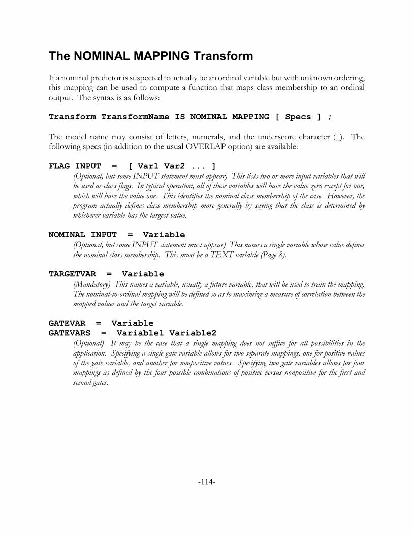
The NOMINAL MAPPING Transform

If a nominal predictor is suspected to actually be an ordinal variable but with unknown ordering,this mapping can be used to compute a function that maps class membership to an ordinaloutput. The syntax is as follows:

Transform TransformName IS NOMINAL MAPPING [ Specs ] ;

The model name may consist of letters, numerals, and the underscore character (_). Thefollowing specs (in addition to the usual OVERLAP option) are available:

FLAG INPUT = [ Var1 Var2 ... ](Optional, but some INPUT statement must appear) This lists two or more input variables that willbe used as class flags. In typical operation, all of these variables will have the value zero except for one,which will have the value one. This identifies the nominal class membership of the case. However, theprogram actually defines class membership more generally by saying that the class is determined bywhichever variable has the largest value.

NOMINAL INPUT = Variable(Optional, but some INPUT statement must appear) This names a single variable whose value definesthe nominal class membership. This must be a TEXT variable (Page 8).

TARGETVAR = Variable(Mandatory) This names a variable, usually a future variable, that will be used to train the mapping. The nominal-to-ordinal mapping will be defined so as to maximize a measure of correlation between themapped values and the target variable.

GATEVAR = VariableGATEVARS = Variable1 Variable2

(Optional) It may be the case that a single mapping does not suffice for all possibilities in theapplication. Specifying a single gate variable allows for two separate mappings, one for positive valuesof the gate variable, and another for nonpositive values. Specifying two gate variables allows for fourmappings as defined by the four possible combinations of positive versus nonpositive for the first andsecond gates.

-114-

IGNORE = ( Value1 Value2 ... )(Optional) It may be that one or more values of the first gate variable indicate an ‘undefined’ condition. These values can be listed here. For cases whose value of the first gate variable equals a value in this list,the output variable is set equal to a neutral ‘median’ value. Values of the second gate variable, if used,cannot be ignored.

MAPPING = MEAN PERCENTILE(Optional, but a mapping method must be specified) For each category (nominal class combined with anygates) the output value generated is equal to the mean percentile rank of all target values in that category. This is usually the preferred mapping, although it does assume that the target mapping carries someinterval information. This is usually a valid assumption.

MAPPING = RANKED PERCENTILE(Optional, but a mapping method must be specified) The MEAN PERCENTILE mapping iscomputed, but the category values are then ranked across all categories. The output value is the percentilerank across categories. This is less powerful than the MEAN PERCENTILE method, but it shouldbe used if no interval information in the target can be assumed.

KEEP Number PERCENTIt may be that only categories that produce extreme responses are considered useful. Those the produceonly a small deviation of the target from its median should be considered noise. This number, less than50 percent, keeps as few classes as possible at each extreme such that at least this percent of cases at eachextreme are represented.

The audit log will contain a table showing the mean target percentile for each category. If a gateis used, the name of the class will be followed by a plus sign to indicate the class correspondingto positive values of the gate, and a negative sign for nonpositive values. If two gates are used,the first sign applies to the first gate, and the second sign applies to the second gate.

-115-

The EXPRESSION Transform

It is possible to use simple arithmetic operations to combine existing variables and/or marketprices to produce new variables. These variables are entered into the database as soon as theyare defined, so it is legal to reference prior computed values in an expression transform. Thesyntax is as follows:

Transform TransformName IS EXPRESSION (MaxLag) [Specs ] ;

MaxLag will be discussed later. There is only one mandatory specification. This is:

TransformName = NumberExpression

This specification must appear exactly once, and it must be the last specification if more thanone is used. The expression defines the arithmetic operations. The name of the computedvariable is the name of the transform.

Here is a silly example:

TRANSFORM DUMDUM IS EXPRESSION (0) [ DUMDUM = 5 ] ;

This will generate a new database variable called DUMDUM which has the value 5 for everycase.

The only other specification available is used to define a temporary variable (not permanentlysaved in the database) that may then appear in the output specification. This is:

TempVarName = Expression

Output or temporary expressions may reference any of the following quantities:

Exis tin g VarNam e - The name of a variable already in the database, or a previously definedexpression, or a temporary variable name

@OPEN : Marke t - This is the opening price of a bar. Market names a market, and it (as wellas the colon) may be omitted if there is only one market. Note that the market musthave been read for this to make sense. @HIGH, @LOW, @CLOSE, and @VOLUMEare also legal. For tick data, all four of the prices will be equal and hence interchangeable.

@OPEN : THIS - As above, except that in a multi-market situation, the market whose priceis used for each record is that record’s market as opposed to being fixed.

-116-

Predefined Variables

Several predefined variables are available for use in expression transforms. These are:

@DATABASE_N - This is the total number of records in the database. If it contains just onemarket, this will be the number of dates (and times if intraday) represented. If there aremultiple markets, this will be the number of unique market/date records.

@DATABASE_POS - This is the number of database records chronologically prior to thiscase. It will range from 0 through @DATABASE_N-1. Note that if there are multiplemarkets, the count of ‘chronologically prior’ records will include records at the currentdate that happen to be prior to this record in the database. The database is always inchronological order, but the order of individual markets at each date is random. Inpractice, as long as there are many more dates than markets, this is of no realconsequence. Ordinal relationship is always preserved: if record A is for a date pastrecord B, then @DATABASE_POS for record A is guaranteed to be greater than@DATABASE_POS for record B. Similarly, if the value of @DATABASE_POS forrecord A exceeds that for record B, then it is guaranteed that record A is notchronologically prior to record B.

@DATABASE_DATES - This is a variant of @DATABASE_POS suitable for multiplemarkets. It is the number of dates for the current market in the database prior to thecurrent record. Thus, it will be zero for the first appearance of this market, one for thesecond appearance, et cetera. Because this variable can be very time consuming tocompute, its maximum value is 20. After 20 appearances of this market, all subsequentvalues of this variable will be 20. This should never be a problem in practice, since theonly reason this variable would be used is for initialization of recursive computations.

These two predefined variables are handy for creating an indicator of time. This is useful in abivariate plot for showing in a single map how the relationship between an indicator and a targetevolves over time. It can also be used in a trivariate plot to extract time slices of the relationshipbetween two indicators and a target. A good way to generate an appropriate indicator of timeis to define it as the percent of the database which has been traversed:

TRANSFORM DB_POS IS EXPRESSION ( 0 ) [ DB_POS = 100 * @DATABASE_POS / (@DATABASE_N - 1) ] ;

The new variable DB_POS ranges from zero for the first (oldest) record, to 100 for the last(most recent) record.

@YEAR - The year of the current record.

-117-

@MONTH - The month of the current record.

@DAY- The day of the current record.

@HOUR - The hour of the current record. This is zero if the data is not intraday.

@MINUTE - The minute of the current record. This is zero if the data is not intraday.

@SECOND - The second of the current record. This is zero if the data is not intraday.

-118-

Basic Operations

Many operations are available. Logical operations always return 1.0 if true and 0.0 if false. Values not equal to zero are treated as true, and zero is false. Common priorities of evaluationare observed, with priorities as shown below. Operations are grouped with dashes (------) fromlast evaluated to first evaluated. However, in case of doubt, use of parentheses is advised.

|| Logical: Are either of the quantities true?&& Logical: Are both of the quantities true?----------== Logical: Are the quantities equal?!= Logical: Are the quantities not equal?< Logical: Is the left quantity less than the right?<= Logical: Is the left quantity less than or equal to the right?> Logical: Is the left quantity greater than the right?>= Logical: Is the left quantity great than or equal to the right?----------+ Sum of the two quantities- The left quantity minus the right quantity----------* Product of the two quantities/ The left quantity divided by the right quantity% Both quantities are truncated to integers; the remainder of the left divided by the right** The left quantity raised to the power of the right quantity----------- Negative of the quantity! Logical: reverses the truth of the quantityABS( ) Absolute value of the quantitySQRT( ) Square root of the quantityCUBERT( ) Cube root of the quantityLOG10( ) Log base ten of the quantityLOG( ) Natural log of the quantityPOWER( ) Ten raised to the power of the quantityEXP( ) Exponentiation (base e) of the quantityATAN( ) Arc-tangent of the quantityLOGISTIC( ) Logistic transform of the quantityHTAN( ) Hyperbolic tangent of the quantity

-119-

Here are a few examples of EXPRESSION transforms:

Compute the difference between two existing predictors:

TRANSFORM DIFF12 IS EXPRESSION (0) [ DIFF12 = X1-X2 ] ;

Compute the high minus the low for IBM:

TRANSFORM HIGHLOW IS EXPRESSION (0) [HIGHLOW = @HIGH:IBM - @LOW:IBM] ;

Compute BIZARRE as X3 if X1>X2, or X4 otherwise:

TRANSFORM BIZARRE IS EXPRESSION (0) [X1BIGGER = X1 > x2X2BIGGER = ! X1BIGGERBIZARRE = X1BIGGER * X3 + X2BIGGER * X4] ;

Here is a pair of expressions from my test suite. The first just sets Exp5 equal to the open ofIBM. The second subtracts the open of each record’s market from Exp5. The resulting quantityExp6 is zero for IBM and more or less random for all other markets.

TRANSFORM Exp5 IS EXPRESSION (0) [Exp5 = @OPEN:IBM] ;

TRANSFORM Exp6 IS EXPRESSION (0) [Exp6 = Exp5 - @OPEN:THIS] ;

-120-

Vector Operations in Expression Transforms

Database variables, market variables, and temporary variables created within the expression maybe referenced with a lag, and they may also be used to generate vectors. To lag a variable,append the lag in parentheses. To generate a vector, append the lag and the vector length inparentheses. For example:

SLOPEVAR ( 5 ) is the variable SLOPEVAR five bars ago in this market.SLOPEVAR ( 0 , 20 ) is a vector of the 20 most recent values of SLOPEVAR in this market.

If a lag and/or vector length results in references to values prior to the first value in the databaseor market, this first value is duplicated as needed to play the role of nonexistent prior values.

When the EXPRESSION transform is declared, the maximum historical lookback (taking intoaccount lags and vector lengths) must be specified. This is an annoyance to the user, but itenables some valuable optimization that saves both memory and execution time. Larger valuesthan required are legal but will cause excessive memory use and slower operation.

When a monadic operator such as SQRT() is applied to a vector, the result is a vector of thesame length in which the operator is applied to each component individually.

When a dyadic operator such as + is applied to a pair of vectors, these vectors should be thesame length. Results are undefined if the lengths are different. The result is a vector of thissame length in which the operator is applied to corresponding elements pairwise.

When a dyadic operator is applied to a vector and a scalar, the result is a vector of the samelength in which the scalar is paired with each element of the vector individually.

The following operations take a vector as an argument and return a scalar:

@MIN ( vec ) - The minimum of all values in the vector@MAX ( vec ) - The maximum of all values in the vector@RANGE ( vec ) - The range (max minus min) of the values in the vector@MEAN ( vec ) - The mean of the values in the vector@STD ( vec ) - The standard deviation of the values in the vector@MEDIAN ( vec ) - The median of the vector@IQRANGE ( vec ) - The interquartile range of the vector@SIGN_AGE ( vec ) - The number of elements in the vector for which the sign remains the

same as that of the first (historically most recent) element. Counting starts at zero. Thevalue zero is treated as negative.

-121-

@PCTILE ( vec ) - The percent of elements in the vector that are less than or equal to the first(most recent) element in the vector. If the first element is the largest, the returned valuewill be 100.0. If the first is the smallest, the returned value will be 100.0 / N where Nis the number of elements in the vector.

@CHAN_NORM - The position of the first (most recent) element in the vector with respectto the range of the vector. This is (Recent - Min) / (Max - Min). If the most recent valueis the minimum, the returned value will be zero. If the most recent value is the largest,the returned value will be one. If all values are equal, the returned value is 0.5.

@SLOPE ( vec ) - The slope per point of a least-squares line fit to the vector@LIN_PROJ ( vec ) - The predicted value of the current point based on a linear fit@SMOOTH ( vec ) - This applies a lowpass filter to the vector. This filter is optimal in the

sense that response is essentially flat until the dropoff knee is reached, at which pointresponse tapers smoothly and quite rapidly to zero and remains essentially zero for allhigher frequencies. Ideally the length of the vector should be odd. If the length is even,the oldest point is ignored. If the length is less than 9, an ordinary moving average isperformed instead of filtering. Let N be the length of the vector, and let H=(N-1)/2. Then the average lag is H, and H is the period at which dropoff begins, the knee of thefilter.

-122-

The following operations take two vectors as arguments and return a scalar. Users should takecare that both vectors are the same length. If they are different lengths, only those casescorresponding to those in the shorter vector are used in computation.

@VECTOR CORRELATION ( Xvec , Yvec ) - The ordinary linear correlation (Pearson R)between the two vectors. This ranges from -1 to 1.

@VECTOR RESIDUAL ( Xvec , Yvec ) - The best linear function for computing the valuesof Yvec from Xvec is computed using ordinary linear regression. This function is usedto predict the most recent case in Yvec using the most recent case in Xvec. Thisfunction returns the actual value minus the predicted value. A frequently useful way tothink of this is to assume that Y is a linear function of X plus a ‘noise’ component. Thiscomponent may not be actual random noise; it may be a nonlinear part of the functionalrelationship, or it may be a source of information contained in Y that is not (linearly)contained in X. This latter interpretation is the most common reason for employing theVECTOR RESIDUAL operation, as the value returned by this operation can then bethought of as the information in Y above and beyond that linearly explainable by X.

@VECTOR RESIDUAL NORMALIZED ( Xvec , Yvec ) - This is identical to VECTORRESIDUAL except that two additional steps are taken after the residual component iscomputed. First, the residual is divided by the standard error of the prediction. This hasthe effect of emphasizing residuals that are produced by very accurate regression, anddriving toward zero residuals that are the result of a poor regression fit. Second, anonlinear function is applied to the standardized residual which compresses extremevalues (which result from exceptionally good linear fits) to a range of -50 to 50.

@VECTOR ALPHA ( Xvec , Yvec ) - The best linear function for computing the values ofYvec from Xvec is computed using ordinary linear regression. This returns the Yintercept of the linear function. In other words, if the linear function is Y = Beta * X +Alpha, this returns Alpha.

@VECTOR BETA ( Xvec , Yvec ) - The best linear function for computing the values ofYvec from Xvec is computed using ordinary linear regression. This returns the slope ofthe linear function. In other words, if the linear function is Y = Beta * X + Alpha, thisreturns Beta.

-123-

Here is an example of using the @SIGN_AGE function in a way that seems reasonable but isnot what is intended. This is followed by a demonstration of how to do it correctly.

Suppose you want to count the number of bars that the variable X is on the same side of its 50-bar moving average. When the current value crosses its moving average, this variable is to havethe value zero. If it then stays on this side of its moving average for the next bar, the valueincrements to one. If it stays there yet again, the value is two. This is to continue up to amaximum count of 20, where it remains if the current value continues on the same side of themoving average. (This sort of truncation is vital to preventing heavy tails.)

On first thought, the following transform may seem reasonable. Note that we look back at 50historical values, including the current. Thus, the maximum lag is 49.

TRANSFORM AGE_A IS EXPRESSION ( 49 ) [ AGE_A = @SIGN_AGE ( X(0,20) - @MEAN(X(0,50)) ) ] ;

Look first at the term @MEAN(X(0,50)). The @MEAN function takes a vector as itsargument. In this case, the vector argument is X(0,50), which is the most recent 50 values ofX. The @MEAN function returns the scalar mean of the vector, which in this case providesthe 50-bar moving average.

This scalar quantity is subtracted from each element of X(0,20), the vector of the 20 most recentvalues of X. Finally, the @SIGN_AGE function counts back from the most recent element ofthis vector, seeing how far it can get before the sign changes (the value crosses the movingaverage). The argument to this function is the value of X minus its 50-bar mean. The valuereturned by this function is the count of how many historical differencess have the same signas the most recent difference.

What’s wrong with this transform? It’s perfectly legal, and it returns a result that may lookreasonable. However, it does not do exactly what you want. This transform computes its count by examining the value of each of the differences between the most recent 20 values of X andthe 50-bar moving average based on a window ending on the current bar. Your goal, as stated atthe beginning of this example, is to examine the difference between a historical case and the 50-bar moving average behind the case being examined as opposed to the moving average behind thecurrent bar.

In order to do this the way you wish, which is also the most sensible way, you need to performtwo transforms in sequence. The first computes the difference between each case and its trailing50-bar moving average. The second counts the sign-change age. This is performed as shownbelow:

-124-

TRANSFORM PRICE_DIFF IS EXPRESSION ( 49 ) [ PRICE_DIFF = X - @MEAN(X(0,50)) ] ;

TRANSFORM AGE_B IS EXPRESSION ( 19 ) [ AGE_B = @SIGN_AGE ( PRICE_DIFF(0,20) ) ] ;

Consider the PRICE_DIFF transform. For each case, it computes the trailing 50-bar movingaverage and subtracts this from the current value of X. Note that if you do not want the currentcase to be included in the moving average, you would use X(1,50) instead of X(0,50). In thissituation, you must bump up the maximum lag from 49 to 50.

The AGE_B transform then examines the series of differences and counts the age of signs.

-125-

Logical Evaluation in Expression Transforms

It is possible to evaluate the truth of a logical expression and choose the execution pathaccordingly. This is done with the following expressions:

IF ( NumberExp ) { Commands executed if NumberExp is nonzero }

ELSE IF ( NumberExp ) { Commands executed if NumberExp is nonzero and all prior if expressions are zero }

ELSE { Commands executed if all prior if expressions are zero }

Note:

1) curly braces {} are required for all logical and looping operations, even if the operationencloses just one command.

2) Logical expressions may be nested.

3) Remember that the final output statement must be the last statement in the transform, so itcannot occur inside a logical expression.

-126-

Here is an example of the use of logical expressions. If long and short trends are both positive,the computed value is +2. If the longer is positive but the short is not, the returned value is +1. The same rules apply for negative trends. Finally, if the longer trend happens to be zero, thereturned value is zero.

TRANSFORM DoubleTrend IS EXPRESSION ( 0 ) [ IF (LIN_ATR_15 > 0) { IF (LIN_ATR_5 > 0) { RETVAL = 2 } ELSE { RETVAL = 1 } } ELSE IF (LIN_ATR_15 < 0) { IF (LIN_ATR_5 < 0) { RETVAL = -2 } ELSE { RETVAL = -1 } } ELSE { RETVAL = 0 } DoubleTrend = RETVAL ] ;

-127-

Special Functions and Variables

The following functions and variables do not readily fit into any of the previous categories:

QUANTILE [ Variable , Fractile ]

The user names a variable that currently exists. This variable may have been computed from theinternal library, or from a prior transform, or read in from an external file. A fractile in the rangefrom zero through one, inclusive, is also specified. This returns the corresponding quantile ofthe variable, the value of the variable which corresponds to the specified fractile. The value ofthis quantile as of any given bar is based on all historical values of the specified variable fromthe first bar through the current bar. Future values of the variable (those later in time than thecurrent bar) play no role in the computation. Note that specifying 0.0 for the fractile returns theminimum of the variable to date, and 1.0 returns the maximum to date.

WINDOW QUANTILE [ Variable , Fractile , Length ]

The user names a variable that currently exists. This variable may have been computed from theinternal library, or from a prior transform, or read in from an external file. A fractile in the rangefrom zero through one, inclusive, is also specified, as well as the length of the historical windowover which the quantile is computed. This returns the corresponding quantile of the variable,the value of the variable which corresponds to the specified fractile. The value of this quantileas of any given bar is based on Length historical values of the specified variable, including thecurrent bar. Future values of the variable (those later in time than the current bar) play no rolein the computation. Note that specifying 0.0 for the fractile returns the minimum of the variableacross the window, and 1.0 returns the maximum.

-128-

Recursive Operations and Lagged Temporary Variables

Some computations require recursion in order to be evaluated. The classic example would beexponential smoothing. In such cases it is vital to use a predefined database variable as shownin an example below in order to properly initialize starting values. If there is only one market,@DATABASE_POS is acceptable for initialization. But @DATABASE_DATES isrecommended for general use, as it produces correct results with multiple markets as well assingle markets. See Page 117 for details.

Here are two equivalent ways to compute a stochastic using an ordinary moving average. Wedon’t need to worry about initialization because references to values prior to the start of theRAW_STOCH series just duplicate the first element in the series.

TRANSFORM STOCH_20_3_A IS EXPRESSION ( 20 ) [ RAW_STOCH = (@CLOSE:OEX - @MIN(@CLOSE:OEX(0,20))) / (@MAX(@CLOSE:OEX(0,20))-@MIN(@CLOSE:OEX(0,20))+0.001) STOCH_20_3_A = (RAW_STOCH+RAW_STOCH(1)+RAW_STOCH(2)) / 3 ] ;

TRANSFORM STOCH_20_3_B IS EXPRESSION ( 20 ) [ RAW_STOCH = (@CLOSE:OEX - @MIN(@CLOSE:OEX(0,20))) / (@MAX(@CLOSE:OEX(0,20))-@MIN(@CLOSE:OEX(0,20))+0.001) STOCH_20_3_B = @MEAN ( RAW_STOCH(0,3) ) ] ;

And here is a similar but not identical way to do this using exponential smoothing. Here we mustdo separate initialization because otherwise TEMP_OUT would not exist the first time itshistorical value is referenced, so there would be no ‘first value’ to duplicate.

TRANSFORM STOCH_20_3_D IS EXPRESSION ( 20 ) [ RAW_STOCH = (@CLOSE:OEX - @MIN(@CLOSE:OEX(0,20))) / (@MAX(@CLOSE:OEX(0,20))-@MIN(@CLOSE:OEX(0,20))+0.001) IF (@DATABASE_DATES == 0) { TEMP_OUT = RAW_STOCH } ELSE { TEMP_OUT = 0.5 * RAW_STOCH + 0.5 * TEMP_OUT(1) } STOCH_20_3_D = TEMP_OUT ] ;

-129-

It is legal but bad practice (due to inefficient internal processing) to make a temporary variablethat is a vector. Thus, the following way to compute a stochastic will give correct results,identical to the first and second examples above. However, it will consume a lot ofcomputational resources (memory and perhaps run time) and so should be avoided wheneverpossible.

TRANSFORM STOCH_20_3_C IS EXPRESSION ( 20 ) [ RAW_STOCH = (@CLOSE:OEX - @MIN(@CLOSE:OEX(0,20))) / (@MAX(@CLOSE:OEX(0,20))-@MIN(@CLOSE:OEX(0,20))+0.001) STOCH_VEC = RAW_STOCH(0,3) // This is the offending line STOCH_20_3_C = @MEAN ( STOCH_VEC ) ] ;

It is illegal to try to convert a vector into a vector. The following expression would cause asyntax error:

TRANSFORM BAD_TRAN IS EXPRESSION ( 10 ) [ X1 = CMMA_5(0,10) TEMP = X1(0,10) // Illegal because X1 is a vector BAD_TRAN = TEMP ] ;

Finally, here is John Ehlers’ 10-bar SuperSmoother as documented on Page 33 of Cycle Analyticsfor Traders.

TRANSFORM SS_10 IS EXPRESSION ( 2 ) [ IF (@DATABASE_DATES < 2) { TEMP_OUT = @CLOSE:OEX } ELSE { TEMP_OUT = 0.12662 * (@CLOSE:OEX + @CLOSE:OEX(1)) + 1.1580 * TEMP_OUT(1) - 0.41124 * TEMP_OUT(2) } SS_10 = TEMP_OUT ] ;

-130-

The LINEAR REGRESSION Transform

It can be useful to use linear regression to combine two or more existing predictors into a singlenew predictor which carries the combined predictive information from the input predictors. Forexample, we might have several measures of volatility. Rather than feeding all of them to amodel, it might be better to find a linear combination of them that has maximum correlationwith a target variable, and feed only this single weighted average to the model. The commandfor computing a linear regression transform is as follows:

Transform TransformName IS LINEAR REGRESSION [Specs] ;

This transform has two mandatory specifications:

INPUT = [ VarName1 VarName2 ... ]This names two or more variables that will take part in a weighted average to compute a new variablethat has a least-squares fit to the target variable.

TARGETVAR = VariableNameThis names a single variable that will be the target for the least-squares fit. This target variable willfrequently be the same target that will be used for training subsequent models, but it need not be. Itdoesn’t even need to be a profit. It can be, for example, a future slope.

The QUADRATIC REGRESSION Transform

This transform is identical to the LINEAR REGRESSION transform except that in additionto the linear terms, squares and all possible cross products are included in the fit. Since thenumber of cross products blows up rapidly as the number of inputs increases, the number ofinputs should be kept small, perhaps even as small as just two. Syntax is as follows:

Transform TransformName IS QUADRATIC REGRESSION [Specs] ;

Note that all linear, square, and cross-product terms take part in the regression. This is incontrast to the QUADRATIC model, in which the terms retained are selected by internal crossvalidation.

-131-

The PRINCIPAL COMPONENTS Transform

This transform is used to perform either principal components analysis or factor analysis bymeans of Varimax rotation of a subset of the principal components.

Suppose we measure two or more indicator variables. In a great many applications, the bulk ofthe variation across cases occurs in a space of dimensionality lower than the space defined byall of the indicators. Also, it is usually this reduced space that contains the majority of the usefulinformation (although notable exceptions do occur).

The more indicators we throw at a model, the more likely it is that we will suffer overfitting. Thus, it may be in our best interest to compute new indicators from a space of reduceddimensionality and use only these indicators in the model. For example, we may measure threedifferent forms of volatility at four different history lengths. This generates twelve indicators. Principal component analysis may let us distill the information contained in these twelveindicators down to just a few new indicators.

Once we’ve defined a reduced dimensionality space, we have a choice for computing newindicators from within that space: rotate or do not rotate. If the indicators will all be fed to alinear model, the choice is unimportant because they will give identical results (except for trivialrounding errors in computation). However, if the reduced set of indicators is given to a linearmodel via stepwise selection, or if they are given to a nonlinear model, the choice can have animpact on performance.

The straightforward and default choice is to stick with principal components. In this case, thefirst new indicator will define the single dimension along which the majority of the variationoccurs across all cases. The second indicator will capture the second-most amount of variationwhich is orthogonal to (uncorrelated with) the first. This repeats for as many dimensions as youdesire.

Optionally, you can request Varimax rotation of the reduced space. You must have at least twodimensions to do this, and it usually makes little sense (although it is legal) to rotate if you havekept all of the original dimensions. This rotation scheme preserves exactly the same informationas is contained in the reduced space before rotation. However, the ordering of most-to-leastvariation is sacrificed in order to (usually) obtain factors that are easier to interpret than principalcomponents. These rotated factors tend to have correlations with the original indicators thatare either near +/- one, or near zero. In other words, rotation tends to produce factors thatrepresent subsets of the original indicators.

-132-

This transform is invoked with the following command:

Transform TransformName IS PRINCIPAL COMPONENTS [Specs] ;

The following specifications may be included:

INPUT = [ VarName1 VarName2 ... ](Mandatory) This names two or more variables that will take part in the dimension reduction.

N KEPT = Integeror

N KEPT = ALL(One of these is mandatory) This specifies how many dimensions to keep. If more than 8 are specified,coefficients for only the first 8 are printed.

ROTATION = VARIMAX(Optional) If specified, Varimax rotation will be applied to the space in order to drive weights towardzero or extremes. If this is not specified, principal components will be output.

Here is a small example from some EWAVES program output. I used four indicators: theclosely related D_COUNT and D_WAVEDAYS variables at degrees 3 and 4. Here is the scriptfile command to do the transform:

TRANSFORM TPC IS PRINCIPAL COMPONENTS [ INPUT = [D_COUNT_3 D_WAVEDAYS_3 D_COUNT_4 D_WAVEDAYS_4] N KEPT = 3 ROTATION = VARIMAX ] ;

This states that we will reduce the dimensionality from four to three, and then perform Varimaxrotation. The following table of factor loadings (correlations between the factors and theoriginal variables) is produced: 1 2 3 Comm

Percent 60.5 34.0 3.5Cumulative 60.5 94.5 98.0

D_COUNT_3 0.811 -0.550 0.005 96.0 D_WAVEDAYS_3 0.789 -0.582 0.000 96.1 D_COUNT_4 0.750 0.606 0.264 100.0 D_WAVEDAYS_4 0.761 0.592 -0.266 100.0

-133-

The following items should be noted in the table just shown:

! The first factor alone accounts for over 60 percent of the variation in the dataset. Thisfactor is essentially a pooled measure of time in a wave, as it has high correlation (around0.8) with all four original indicators.

! The second factor accounts for another 34 percent of the variation. These first two newindicators together account for almost 95 percent of the total variation! This factor haspositive correlation with the two Degree-4 indicators, and negative with the two atDegree 3. In other words, it is a measure of the contrast between what’s happening atDegree 4 and what at Degree 3.

! The third factor accounts for only 3.5 percent of the total variation. It contrasts the twodifferent measures of wave time at Degree 4. It essentially ignores Degree 3.

! The last column in a loading chart is always Communality. This is the percent ofvariation of each original indicator that is captured in the reduced space. Note that thisreduced space captures all of the Degree-4 variation, and almost all of that at Degree 3.

Because the ROTATION = VARIMAX option appeared, the program also displays the rotatedloading matrix: 1 2 3 Comm

Percent 48.1 46.4 3.5Cumulative 48.1 94.5 98.0

D_COUNT_3 0.968 0.153 0.001 96.0 D_WAVEDAYS_3 0.973 0.115 0.006 96.1 D_COUNT_4 0.134 0.957 -0.256 100.0 D_WAVEDAYS_4 0.149 0.950 0.274 100.0

-134-

Note the following aspects of the rotated loadings:

! After rotation, we still capture 98 percent of the total variation. Rotation does notchange the total, although the individual factors need not remain ordered largest tosmallest.

! The communalities always remain the same after rotation. This is because it’s still thesubspace. Only the axes have rotated.

! After rotation, the first factor (the largest here only by chance; order is lost after rotation)essentially tells us what’s going on at Degree 3. The second factor captures informationfrom Degree 4. The third is pretty much unchanged by the rotation.

Remember that rotation does not alter the information content of the reduced set. It onlychanges how we look at it and how we compute the new indicators.

Finally, it may (rarely) be interesting to see the actual coefficients that are used to transform thestandardized original indicators into the new factors. Note that these will often be quitedifferent from the loadings, which are correlations, not weights. Here is the score coefficientmatrix: 1 2 3

D_COUNT_3 0.521 -0.066 -0.034 D_WAVEDAYS_3 0.530 -0.090 0.001 D_COUNT_4 -0.069 0.552 -1.877 D_WAVEDAYS_4 -0.078 0.518 1.897

-135-

The ARMA Transform

An ARMA (autoregressive, moving average) model can be fit to a moving window in thedatabase or a market, and any of several quantities can be computed to generate a new databasevariable. The ARMA transform is invoked as follows:

Transform TransformName IS ARMA [Specs] ;

The following specifications may be included:

SERIES = SourceThis specifies the series which will be fit with an ARMA model. The following sources are available:VarNam e - The name of a variable in the database. If multiple markets are present, each marketwill be processed independently.VarNam e :Marke t - The name of a variable in the database, using values in the specified market. If multiple markets are present, the specified market’s computed values will be cloned onto each market.@CLOSE - The close of the market will be used. Legal only if there is just one market.@CLOSE:Marke t - The close of the named market will be used.For the above market series, @OPEN, @HIGH, @LOW, and @VOLUME are also legal.

ARMA WINDOW = IntegerThis specifies gives the length of the data window. If the ARMA model has only one parameter, awindow length of as little as 20 is acceptable, although larger windows, such as 100, are more stable. If two parameters are estimated, a window length of 100 should be considered a minimum.

AR = IntegerThis specifies the number of AR parameters.

MA = IntegerThis specifies the number of MA parameters.

ARMA OUTPUT = TypeThis specifies the value that will be generated for the database. The following types are available:PREDICTED - The predicted value of the last case in the windowSHOCK - The shock experienced by the last case in the windowSTANDARDIZED SHOCK - The shock divided by the standard deviation of shocksMSE - The mean squared error (variance of the shocks) in the windowRSQUARE - The fraction of series variance that is predictable by the ARMA modelAR PARAMETER In te g e r - The value of the trained AR parameter at the integer lagMA PARAMETER In te g e r - The value of the trained MA parameter at the integer lag

-136-

ARMA TRANSFORM = LOGThis optional specification decrees that the source series will be transformed by taking natural logs beforethe ARMA model is fit. The source series must be strictly positive.

ARMA TRANSFORM = DIFFERENCEThis optional specification decrees that the source series will be differenced before the ARMA model isfit. Differencing will often remove or greatly decrease nonstationarity of the mean of a series.

ARMA UNDO TRANSFORMThis option makes sense only if at least one of the above transforms is performed and the output is eitherPREDICTED or a SHOCK. If this option is not used, the predicted value (and hence the derivedshock) remains in the transformed domain. If this option is used, the transform is undone for theprediction, and the shock computed accordingly. Note that if the only transform is a difference, the shockwill be the same regardless of whether or not the transform is undone.

For example, the following transform will fit an ARMA model containing just one AR parameter(a common, stable, and usually effective model; an excellent first choice) and create a newindicator whose value is the AR parameter, which indicates the degree and sign of lag-one serialcorrelation in the closing value of OEX. This may be useful predictive information because itindicates whether the market is in a trending or mean-reversion mode. Since this is a market,it makes sense to first do a log transform and then difference so that the ARMA model isoperating on changes, not actual values.

TRANSFORM OEX10_LD_AR IS ARMA [ SERIES = @CLOSE:OEX ARMA WINDOW = 100 ARMA TRANSFORM = LOG ARMA TRANSFORM = DIFFERENCE ARMA OUTPUT = AR PARAMETER 1 ARMA AR = 1 ARMA MA = 0 ] ;

-137-

The PURIFY Transform

It is a universal fact of life in predictive modeling that useful predictive information in anindicator is diluted by variability attributed to other, less relevant phenomena. Such phenomenamay contribute little or no useful predictive information, and hence be essentially noise. If thedeveloper is able to identify a potential source of the noise pollution, it may be possible toremove it and thereby purify the original indicator, increasing its predictive power.

The method for doing this is straightforward: first one must identify a series, measuredconcurrently with the ‘polluted’ indicator, which is believed to be a source of pollution. Thisseries, called the purifier, may be prices of a market, or an indicator itself, or some other marketmeasure such as volume or open interest. Then apply one or more moving-window functionsto the purifier series. Find a model (linear is fast and easy) which does a decent job of usingthese functions of the purifier to predict the indicator being purified. Finally, subtract thepredicted values of the indicator from the actual values of the indicator. This predicted valueis, to at least some degree, the pollutant. Thus, subtracting it from the series to be purified hasthe effect of reducing the pollution in the indicator, leaving behind a higher concentration ofuseful information.

The following command is used to purify a series:

TRANSFORM TransformName IS PURIFY [Specs] ;

Some of the specifications are mandatory, and others are optional. All possible specificationsare now discussed, grouped by their uses.

Defining the Purified and Purifier Series

The user must specify two series. These are the series to be purified, and the purifier series. As with all transforms, the generated output series is given the name of the transform,TransformName, in the definition. The purified and purifier series may be any of the following:

! The open, high, low, close, or volume of a market. The purified series is invariablyan indicator, not actual trading prices of a market. Nonetheless, it is often advantageousto either read these two series as TSSB markets (READ MARKET HISTORIES) or letthem be ‘markets’ that have been operated on by a prior transform. Computing themfrom the built-in library, or reading them in from an external database, can, in someinstances, deprive the user of valuable early history information. This will be discussedin detail later in this section.

-138-

! An indicator computed from the built-in library. If this is done, the length of earlyhistory available to the transform will be reduced by the maximum lookback in thevariable definition list (READ VARIABLE LIST). If any internally computed indicatorhas a longer lookback than the indicator(s) needed for the purified or purifier series, datawill be wasted. Thus, use of the internal library may better be done in a separate scriptfile if available history is limited. The separately computed indicators and the PURIFYtransform values can be merged for training and testing of trading systems by means ofan APPEND DATABASE command.

! A variable read in from an external data file with the APPEND DATABASEcommand. If this is done, the user should ensure that the external data file starts at asearly a date as possible in order to maximize the length of history available to thetransform. The appending is done before transforms are computed, so even if extensivehistorical data is available prior to appending, if the appended data file starts at a laterdate, the previously available data will become unavailable. Also, realize that thePURIFY transform, like all transforms, preserves market associations. Thus, the file readshould contain data for any market(s) that will ultimately be traded.

Exactly one PURIFIED and one PURIFIER specification are required. The followingcommands are used to define the purified and purifier series:

PURIFIED = @close:MarketNameThis names a market whose close will be purified. It is also legal to use the ‘open’, ‘high’, ‘low’, or‘volume’ of a market. Because the purified series is virtually always an indicator, in practice this serieswill not actually be trading prices of a market. Rather, it will be an indicator that is read in as if it werea market by means of the READ MARKET HISTORIES command. Usually this is the bestapproach because this method provides the most history to the transform, and also because data read inas a TSSB market is automatically cloned to all markets named in the READ MARKET LISTfile, which simplifies model training and testing.

PURIFIED = VariableNameThis names an indicator that will be purified. This indicator may have been computed from the built-inlibrary, or computed from a prior transform in the script file, or read in from an external database. Onepowerful technique which gives the user great versatility but does not generally cost availability of historicaldata is to read in a variable as a TSSB market, apply an expression transform, and then use the resultof this expression transform as the purified or purifier series.

PURIFIER = @close:MarketNamePURIFIER = VariableName

The same considerations just discussed for the purified series apply to the purifier series, with one smallexception. The only difference is that although the purified series will nearly always be an indicator, thepurifier series will often be actual market price history.

-139-

PURIFY USE LOG PURIFIERThis optional command decrees that the natural log of the purifier series will be taken before predictorfunctions are computed from the series. This is usually appropriate when the purifier series is marketprice histories, and usually not needed when the purifier series is an indicator.

Specifying the Predictor Functions

The user must specify at least one predictor function and at least one lookback length for thepredictor function(s). The user must also specify whether one or two predictors are to be usedin the linear model that uses the functions to predict the purified series. The relevantspecifications are the following:

PURIFY N PREDICTORS = IntegerThis is the number of predictors (functions of the purifier series) that the purification model will use topredict the purified series. It must be 1 or 2. If 2 is specified, all possible pairs of predictors will betested, so execution time could be slow if the user employs numerous predictor candidates.

PURIFY LOOKBACKS = ( Integer Integer ... )This list of one or more integers specifies the lookbacks (window lengths) in the purifier series to use whencomputing the predictor functions. Each must be at least 3. This specification must appear if anypredictor function other than VALUE (defined below) is used.

PURIFY PREDICTOR FAMILY = TRENDThis makes available to the purification model the linear trend of the purifier series, measured over eachlookback distance given in the PURIFY LOOKBACKS specification.

PURIFY PREDICTOR FAMILY = ACCELERATIONThis makes available to the purification model the quadratic component (rate of change in trend) of thepurifier series, measured over each lookback distance given in the PURIFY LOOKBACKSspecification.

PURIFY PREDICTOR FAMILY = ABS VOLATILITYThis makes available to the purification model the volatility of the purifier series, measured over eachlookback distance given in the PURIFY LOOKBACKS specification. The volatility here is theexponentially smoothed absolute change.

PURIFY PREDICTOR FAMILY = STD VOLATILITYThis makes available to the purification model the volatility of the purifier series, measured over eachlookback distance given in the PURIFY LOOKBACKS specification. The volatility here is thestandard deviation of the changes in the purifier series, annualized by multiplying by sqrt(252).

-140-

PURIFY PREDICTOR FAMILY = Z SCOREThis makes available to the purification model the moving z-score of the purifier series, measured overeach lookback distance given in the PURIFY LOOKBACKS specification. The z-score is found bycomputing the mean and standard deviation of the purifier series across the lookback window, subtractingthe mean from the current value of the series, and dividing by the standard deviation. Nonlinearcompression combined with hard limiting is used to prevent extreme values due to tiny standarddeviations.

PURIFY PREDICTOR FAMILY = SKEWThis makes available to the purification model an order-statistic-based measure of skewness.

PURIFY PREDICTOR FAMILY = VALUEThis predictor specification is different from all of the others. The VALUE predictor makes availableto the purification model the current value of the purifier series. It is not a function, and hence lookbackdistance is irrelevant. The VALUE option would almost never make sense when the purifier series ismarket price history. However, it may be that the user has contrived a special predictor for thepurification model, a predictor that is designed to be used itself, as opposed to functions of it being used. In this case, the VALUE predictor would be specified. The PURIFY USE LOG PURIFIERoption is ignored for the VALUE predictor; the actual value is always used.

Miscellaneous Specifications

This section discusses the PURIFY transform specifications that do not fit in the priorcategories. These are as follows:

PURIFY WINDOW = IntegerThis mandatory line specifies the number of cases (the lookback length) that are used to train thepurification model. It must be at least 3, and is usually much larger, perhaps as much as severalhundred.

PURIFY NORMALIZE = PERCENTBy default, the output of the PURIFY transform is the actual value of the purified series minus thepredicted value. But if the PURIFY NORMALIZE = PERCENT option appears, this differenceis divided by the absolute value of the purified series and then multiplied by 100. This expresses thedifference as a percent of the actual value. If, as is often the case, the local standard deviation of thepurified series is proportional to its absolute value, the PERCENT normalization can stabilize thevariance of the transform output. Note that purifying the log of such a series also produces variancestabilization, and usually does so better than the PERCENT option.

-141-

PURIFY NORMALIZE = STDERRBy default, the output of the PURIFY transform is the actual value of the purified series minus thepredicted value. But if the PURIFY NORMALIZE = STDERR option appears, the difference isdivided by the standard error of the estimate produced by the purification model. Note that near thebeginning of the available history, when the model has incomplete information, the standard error candrop to near zero, producing huge z-scores. For this reason, the output of the PURIFY transform isstrongly constrained near the beginning of the data series, and moderately constrained thereafter to preventextreme values that can hinder subsequent model training.

PURIFY OUTPUT = FIRST PREDICTORThis option is for diagnostic purposes only. It disables purification. The output of the PURIFYtransform when this option is employed is the first PURIFY PREDICTOR FAMILY variablenamed in the option list, computed at the first lookback in the PURIFY LOOKBACKS list. Forexample, suppose the user had the following option as the first predictor: PURIFY PREDICTORFAMILY = Z SCORE. Then the output of the transform would be the exact z-score values used aspredictors by the purification model. Subsequent predictors and lookbacks other than the first in the listare ignored. This option can occasionally be a handy way to inspect the predictors in order to verifyvisually (or even numerically) that they look like what you expect them to look like. It’s unlikely thatcasual users would ever employ this option.

Usage Considerations

The PURIFY transform is integrated into the train/test cycle like other transforms, and it mostlybehaves the same as others. However, there are two aspects of the nature of purification itselfthat merit special consideration.

First, purification almost always has a very long total lookback length. It requires extensivehistory before it has the full amount of data needed to meet the user’s specifications. This isbecause two windows are involved. At the outermost level we have the PURIFY WINDOWlookback which tells the transform how many cases will go into training the purification model. Then, for each case in this window, we have the windows for computing the predictor variables,the longest of which in the PURIFY LOOKBACKS list may be quite long. So when computingthe purified value of any record (bar of data in a market), the oldest case in the training set forthe purification model will be back in history by the PURIFY WINDOW distance, and in orderto compute the predictors for this case we will need an additional historical window whoselength is the longest lookback in the PURIFY LOOKBACKS list. It’s not unusual to need atotal lookback of several years, which is substantial if data is limited. Computation does beginimmediately, without waiting for the full lookback to be reached. However, the first few valueswill be seriously in error due to massive lack of data, and it will probably be on the order of ahundred or so records before accuracy becomes even marginally usable. Full accuracy is notobtained until the entire total lookback distance is reached.

-142-

For this reason we are inspired to make as much history as possible available to the PURIFYtransform. In most situations the easiest way to do this is to do the purification alone, in a singlescript file, and write the purified series as a database using the WRITE DATABASE command. Read both the purified and the purifier series as TSSB markets. Have a token variable list,probably containing just one variable definition which has an extremely short lookback. (Thisis needed because the current version of the program requires that either a variable list ordatabase have been read before any transform is done. This requirement may be eliminated ina future version.) It is perfectly legitimate and often useful to then apply one or more expressiontransforms to the ‘markets’ read, and then purify the output of the transform. This does notcause the loss of history, so it is innocuous. On the other hand, early history of a length equalto the longest lookback in the variable definition list will be eliminated, which is why we wantto keep the lookback in the variable definition list very short.

If the trading model(s) being developed require other indicators, they can be computed in aseparate script file and saved to a database. Their lookbacks will cost market history, but that’snot a problem, because the purification will have been done separately, and the history lost dueto lookbacks from the internal indicator library will just be early ‘warm-up’ data in the purifiedseries, data that is probably best discarded anyway!

Of course it’s legal for the purified and/or purifier series to be computed from the internallibrary, or read in from an outside source with an APPEND DATABASE command. Just beaware of the potentially long lookback requirement of purification and try hard to providehistorical data that begins at as early a date as possible.

The second issue of purification is that the purified and purifier series must be preciselyconcurrent in history if full accuracy is to be maintained. Suppose one series has missing dataon a certain date. Then even though the ending dates of the two series are aligned to the‘current’ date, the two series will remain aligned only as far back as the missing data. After that,the measurement dates of the two series will become misaligned and accuracy can suffer.

In order to prevent this from happening, the first time a PURIFY transform is encountered inthe script file the database will be preprocessed to eliminate any dates that do not have a fullcomplement of markets. When this happens, a line similar to the following will appear in theaudit log:

Removing database records with incomplete markets reducedcases from 11924 to 11918

In this example, the database originally contained 11924 records, but 6 of them did not have acomplete set of records, leaving 11918 complete dates. This is a one-time operation.

-143-

A Simple Example

We now examine a simple two-part example. The first script file purifies the log of a ‘market’called VIX, and the second file uses the purified value to make trade decisions. Here is the firstscript file:

READ MARKET LIST "OEX_VIX.TXT" ;READ MARKET HISTORIES "E:\SP100\OEX.TXT" ;READ VARIABLE LIST "VARS_PURIFY_DEMO1.TXT" ;

TRANSFORM LOG_VIX IS EXPRESSION ( 0 ) [ LOG_VIX = LOG ( @CLOSE:VIX ) ] ;

TRANSFORM PURIF_LOG IS PURIFY [ PURIFIED = LOG_VIX PURIFIER = @close:OEX PURIFY USE LOG PURIFIER PURIFY WINDOW = 300 PURIFY LOOKBACKS = ( 11 22 44 65 130 260 ) PURIFY N PREDICTORS = 2 PURIFY PREDICTOR FAMILY = TREND PURIFY PREDICTOR FAMILY = ACCELERATION PURIFY PREDICTOR FAMILY = VOLATILITY PURIFY PREDICTOR FAMILY = Z SCORE ] ;

TRAIN ;

WRITE DATABASE "T_PURIFY_DEMO2.DAT" ;

The market list OEX_VIX.TXT contains only two markets: VIX, which is the market sentimentseries which will be purified, and OEX, the market index that will be the purifier series.

The variable list VARS_PURIFY_DEMO1.TXT contains only one token indicator:DUMMY: LINEAR PER ATR 3 5

VIX tends to have a standard deviation proportional to its magnitude, so taking its log beforepurification stabilizes its variance, which is a crucial property of stationarity. Like all transforms(except ARMA), the expression transform used to compute the log of VIX does not cost anymarket history.

-144-

The purifier series is the close of OEX, and its log will be taken before any predictor functionsare computed.

The purification model will be trained with a moving window of 300 cases. For each case in thatwindow, six different lookbacks, ranging from 11 through 260, will be used to compute thepredictor functions.

The model will be given the four named predictor functions, each evaluated at each of the sixlookbacks, making a total of 24 predictor candidates. The two best predictors will be found.

The TRAIN command causes the purification to be performed across the entire database atonce, and the results will be written to a database file.

Here is the second part of this example, in which the database just created is read, and a tradingmodel is walked forward:

READ MARKET LIST "OEX.TXT" ;READ MARKET HISTORIES "E:\SP100\OEX.TXT" ;READ VARIABLE LIST "VARS_PURIFY_DEMO2b.TXT" ;APPEND DATABASE "T_PURIFY_DEMO2.DAT" ;

MODEL MOD_PURIF IS LINREG [ INPUT = [ PURIF_LOG ] OUTPUT = RETURN MAX STEPWISE = 0 CRITERION = PROFIT FACTOR MIN CRITERION FRACTION = 0.1 RESTRAIN PREDICTED ] ;

WALK FORWARD BY YEAR 10 2000 ;

This time, the market list contains only one market, OEX. This is because we want to trade onlyOEX in this example. If VIX, as it exists in the market history file, were tradeable and the filecontained the actual trading prices, we might (or might not) be interested in also including it inthe market list. If this were done, all performance results would include trades in VIX as wellas OEX.

The new variable list VARS_PURIFY_DEMO2b.TXT contains just one line:

RETURN: NEXT DAY ATR RETURN 252

-145-

This variable is needed because it is the target for training and testing the model. It would havebeen legal to place this line in the variable definition list for the first half of this example, inwhich the purification was done. If so, the RETURN variable would have been computed there,written to the database, and read in this example, saving the trouble of having this separatevariable list. However, the RETURN variable has a lookback of 252 days. If it had beencomputed in the purification script, its entire lookback of 252 days would have been unavailableto the purification transform, a significant loss.

After this one-line variable list is read, we append the database that was computed in the firsthalf of this example. This contains the purified VIX for both the OEX and VIX markets. However, since the existing database contains only OEX, all VIX records will be eliminatedduring the APPEND operation, leaving the model to be trained and tested on only OEX.

The model is trained and tested using purified VIX as the sole indicator, and RETURN as thetarget. The CRITERION is irrelevant because it is used for stepwise selection only, and this isa single-indicator model. Nonetheless, it must be included in any model definition.

Finally, the model is walked forward from 2000 using 10-year training sets.

-146-

The Hidden Markov Model Transform

When working with variables derived from market data, the developer need not assume a directrelationship between predictors and a target. Sometimes it is better to posit an underlyingcondition, the state of the market, which impacts both the predictors and the target. Thisprocess is assumed to exist at all times in exactly one of two or more possible states. The stateat any given time impacts the distribution of associated variables. Some of these variables maybe observable at the present time (predictors, computed from historical data), while others maybe unknown at the present time but be of great interest (targets, based on future marketmovement). Our goal is to use measured values of the observable variables to determine (ormake an educated guess at) the state of the process, and then use this knowledge to estimate thevalue of an unobservable variable which interests us.

It is vital to distinguish this application from ordinary classification methods which are notrestricted to time series data. In simple classification, one measures some predictor variable(s)and makes a class decision, which in turn may imply likely values of other (probablyunmeasurable) variables. But a hidden Markov model assumes a sequential process with animportant property: the probability of being in a given state at an observed time depends on theprocess’s state at the prior observed time. In other words, a hidden Markov model has memory,while ordinary classification does not.

This memory is immensely useful in some applications. For example, it may prevent whipsaws. Suppose a certain market state tends to be persistent. Ordinary classification will suffer if thereis large random noise in the predictors, which may snap the state decision back and forth at thewhim of chance. But the memory inherent in a hidden Markov model will tend to hold its statedecision in a persistent state even as noise in the predictors tries to whip the decision back andforth. Of course, the downside of this memory is a tendency toward delayed decisions; themodel may need several observed values to confirm a market state change. But this is often aprice well worth paying, especially in high-noise situations such as trading financial markets.

For example, suppose the developer assumes that it is always in either a bull market (a long-termup-trend), a bear market (a long-term down-trend) or a flat market (no long-term trend). Bydefinition, bull and bear markets cover an extended time period; one does not go from a bull toa bear market in one day, and then return to a bull market the next day. Such direction changesare just short-term fluctuations in a more extensive move. If one were to use frequentobservations to make daily predictions of whether the market is in a bull or bear state, thesedecisions could reverse ridiculously often. One is better off taking advantage of the memory ofa hidden Markov model to stabilize behavior.

There are several aspects of hidden Markov models that merit special consideration when usedin TSSB or any other application that involves moving windows. In practice, these issues have

-147-

little or no practical impact when properly respected, but the user must be aware of them inorder to avoid making a grave error or misunderstanding perplexing results.

First, hidden Markov models are very difficult to train, as they have numerous local optima. Forthis reason, a starting point for the hill-climbing training algorithm is located by testing a largenumber of randomly chosen points and selecting the best as the starting location for training. The practical impact of this fact is that results are not always exactly reproducible. If trainingis done twice, the exact definition of the model may be different in the two runs. Because ahuge number of trial starting points are tested, it is unlikely that the models will differ much intheir power; the training algorithm nearly always converges to an excellent optimum. But thisis not like linear regression, in which model coefficients are computed by an explicit formula. There is inherent randomness in hidden Markov models, so variations in model parameters areto be expected.

Second, assignment of state identity to meaningful state properties is random. For example, wemay define a two-state model based on recent trend, with the idea that one state represents arising trend and the other state represents a falling trend. It may happen that the first time wetrain the model, the first state will correspond to the rising trend and the second state willcorrespond to the falling trend. If we train the model again, we may find that the first statecorresponds to the falling trend and the second state corresponds to the rising trend. This is anatural result of the random nature of training.

Needless to say, this would have disastrous consequences in a moving-window situation if notdealt with. Imagine if the training data for a model had a random mixture of state associations,with State 1 representing an upward trend one day, and this same state number representing adownward trend the next day! The model would be worthless. We will soon see how TSSBmakes such random reassignments extremely unlikely, though not impossible.

Third, the training algorithm for hidden Markov models involves numerous bidirectional sweepsthrough the data; first it passes through the window in a forward direction to the end, then itsweeps back to the beginning. As a result, the entire training window contains massive futureleak; state decisions made for early data points are impacted by values of the data all the way tothe end of the training window.

All three of these potentially devastating properties of hidden Markov models are handled inTSSB by means of a specialized computational procedure. The initial training window is placedat the start of the data and the model is trained. This window will contain enormous future leak,so the out-of-sample period must be entirely past this point. For the user’s convenience, TSSBprints the last date in this window, an example of which is shown below. Training data may liein this window, but the first walkforward out-of-sample date must be beyond it.

Last date in initial window is 19930820

-148-

After an optimal model for this window is computed, the window will be advanced by just onebar (regardless of any walkforward parameters specified by the user). Then the model will beretrained. But instead of again starting the training from a randomly selected near-optimal point,it will be started from the existing model’s parameters. Since the change in the data is slight, thechange in the model should also be slight. For example, suppose the training window is 1000bars, a reasonable length. Then 999 of the window points will be the same; only one point willchange. As a result, it is extremely unlikely that the assignment of state identities to stateproperties will change; if State 1 corresponded to particular properties of the indicators, it willcontinue to correspond to the same properties after the window is advanced and the model isretrained.

Once the window has advanced by one bar, then the state of the most recent bar will berecorded. But the states of prior bars will not be adjusted, even though some of them will likely changealong with the updated model. In this way, future leak is avoided. Once we are outside theinitial window, the state classification at any given bar depends on only data that is known upto that bar.

Despite this algorithm, in pathological situations it is possible for state assignments to switch,with potentially serious consequences. This is most likely to occur when the data goes througha time period in which a hidden Markov model does not adequately describe the data within thewindow. For example, suppose the user posits an up-trend and a down-trend and chooses oneor more indicators accordingly. It is likely that the initial window will contain numerous localup-trends and down-trends, and the model will find and fit them well, quickly associating thetwo state identifiers with the two apparent states. But now suppose that as the window moves,a time comes when the variation in the trend indicator(s) nearly vanishes, most likely due to anextended flat market. The difference in the states, as measured by the indicator(s), becomesvanishingly small; a hidden Markov model is no longer a good way to explain the indicatorvalues. Once this happens and trend variation reappears, it’s a coin toss which way the stateassignments will be made. If it happens to reverse, the user might be left with a nonsensicaltraining set, one in which an up-trend is associated with one state in part of the training periodand the other state in the remainder of the training period. This can be disastrous.

How can we ensure that this does not happen? It is impossible to guarantee it will not occur,but there is one simple way to reduce its probability to minuscule levels, as well as a way tousually detect it when it does happen. The solution is to use as long a window as possible, withat least 1000 bars being recommended. This has two effects. First, it nearly guarantees only tinychanges to the model as the window moves. Changing just one data point while keeping 999the same means that only tiny tweaks will be made to the model as the window moves, makinga complete reversal of state assignments extremely unlikely. Perhaps even more important, along window makes it unlikely that the model will become irrelevant across the window’s entireextent. If the window contains just 50 bars, it is possible, even likely, that a time will come whenthe market remains in just one state (as far as the indicators are concerned) for its entire extent.

-149-

For example, an up-trend-down-trend model based on 50-bar windows could easily be stymiedwhen the market goes flat for 50 bars. But the probability of a market going flat for 1000 barsis nearly zero. Some part of the window will still have variation in trend, and the model willtherefore remain intact.

Despite the use of a long window, it is rarely possible for a model to switch state assignments. An easy way to detect this is to compute and plot the mean of the indicator for each state andconfirm that the plotted means never cross. Of course, the random, non-repeatable nature ofthe training process means that it may even happen that the training run that produced the plotsof means may not represent the training process that produced the state memberships. But thiswould be extremely rare, especially if the window is long. Examining plots of state means isalways advisable. If nothing else, it may reveal time periods in which the means becomeperilously close, in which case one should realize that the indicator(s) chosen may not be the bestway to categorize the market across its entire extent. Excellent indicators will have their statemeans well separated for the entire market history.

Outputs Generated by the Transform

As with other transforms that produce multiple outputs (such as principal components), thehidden Markov model transform produces outputs that are the name given to the transformfollowed by an integer beginning at 1. There will be as many outputs as classes (market states)specified by the user. For example, suppose the user creates an HMM transform called TH andspecifies that three states are to be assumed. Then the outputs created will be TH1, TH2, andTH3.

-150-

Specifying the Parameters for the Hidden Markov Model

The following command is used to declare a hidden Markov model transform:

TRANSFORM TransformName IS HMM [Specs] ;

The legal specifications are shown below:

HMM CLASSES = NumberThis specifies the number of classes (market states). TSSB imposes an upper limit of 5, but 2-4 aretypical, with more classes leading to more unstable behavior. Of course, it must be at least 2.

HMM WINDOW = NumberThis specifies the length of the moving window. It should be as large as possible, with at least 1000 beingrecommended to minimize the probability of assignment switches.

HMM PREDICTOR = [ Variable1 Variable2 ... ]This lists the indicators which will define the market states. TSSB imposes an upper limit of 8, whichis far more than would ever be used in practical applications. In fact, just one indicator is often sufficientto accomplish what the user desires, and two indicators should be sufficient for nearly every application. If multiple markets are present, the market for each indicator must be specified by following the indicatorname with a colon and the market name. An example of this appears later.

HMM OUTPUT = MEMBERSHIPThis specifies that the output variables will be the membership probabilities of each market state. Theywill, of course, sum to one, so if there are two classes then either one of the two output variables issufficient to convey all state information. This option is the fundamental output of the HMM transform.

HMM OUTPUT = MEANThis specifies that the output variables will be the mean of the first predictor for each class. There is noway of outputting the means for variables other than the first listed in the HMM PREDICTORstatement. However, it is perfectly legitimate to use more than one HMM transform, with the predictorsspecified in different orders, if means for each are to be computed. The usual purpose for this output isto plot the state means across time and confirm that they remain well separated. If they come close, thenthe user might wish to reconsider the indicator, as it is not definitive across the entire history. If the statemeans ever cross, the model has switched state assignments and should be entirely redesigned. This shouldalmost never occur if the window is sufficiently long. The difference between state means may serve as anovel regime indicator itself.

HMM OUTPUT = STDDEVThis is identical to the OUTPUT=MEAN command except that the outputs are the standarddeviations.

-151-

HMM OUTPUT = TRANSPROBThis specifies that the outputs are the probabilities that the market state remains in the same state.

Example Outputs

Figures on the next few pages illustrate the various outputs available. In all cases, the userspecifies HMM CLASSES=2, so two market states are assumed.

Figures 4 and 5 are the membership probabilities. Naturally they sum to one. It is interestingto note that the model is only rarely unsure of itself. Most of the time the probabilities are nearzero and one.

Figures 6 and 7 are the state means. Note that although they vary greatly across the markethistory, they always remain well separated, which is a sign of stability. If the user ever observesstate means that come perilously close at some point, this indicates that the indicator(s) areprobably not well associated with a Markov process. If the means ever cross, this is serioustrouble and different indicators should be chosen. Using a larger window will often remedy thisproblem. Sometimes the difference in state means can be a useful regime indicator, althoughits variation is typically so slow that it can be problematic. Daily changes in the state meandifference are often useful as well.

Figures 8 and 9 are the state standard deviations.

Figures 10 and 11 are the probabilities of remaining in each of the states, the diagonal elementsof the state transition matrix.

-152-

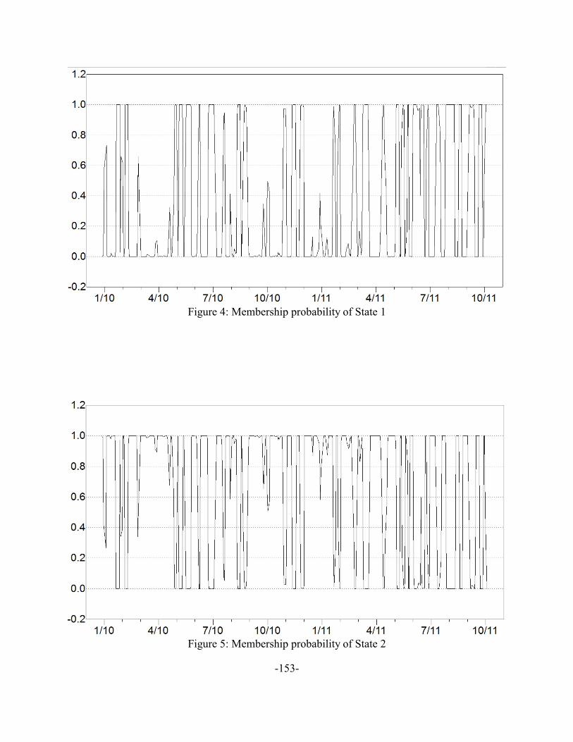
Figure 4: Membership probability of State 1

Figure 5: Membership probability of State 2

-153-

Figure 6: Mean of State 1

Figure 7: Mean of State 2

-154-

Figure 8: Standard deviation of State 1

Figure 9: Standard deviation of State 2

-155-

Figure 10: Probability of remaining in State 1

Figure 11: Probability of remaining in State 2

-156-

Example Applications of Hidden Markov Models

The first step in using a hidden Markov model transform will nearly always be to declare thetransform, execute it with a TRAIN command, and write the results to a database which canthen be read in as needed later. The HMM transform integrates correctly into the train/testcycle, so it is legal to compute it in a walk-forward run. But this would nearly always be foolish,as the transform is very slow to compute. It makes much more sense to compute it just onceand save the results. Another benefit of this approach is that results will then be consistent. Ifthe HMM transform is recomputed for every application, the random nature of the trainingprocess will likely introduce small but annoying variation in performance results. Exactreproducability is a wonderful virtue in an experiment.

Here is an example script file to compute and save membership probabilities:

READ MARKET LIST "SYM_OEX.TXT" ;READ MARKET HISTORIES "E:\SP100\OEX.TXT" ;CLEAN RAW DATA 0.3 ;READ VARIABLE LIST "VARS_3.TXT" ;

TRANSFORM HMM_MEMBERSHIP IS HMM [ HMM PREDICTOR = [ LIN_ATR_5 LIN_ATR_15 ] HMM CLASSES = 2 HMM WINDOW = 1000 HMM OUTPUT = MEMBERSHIP ] ;

TRAIN ;

WRITE DATABASE "HMM.DAT" "HMM.FAM" ;

Once the membership probabilities have been computed and saved, they can be read back forvarious experiments. In the example just shown, all necessary predictors and targets werecomputed and saved along with the HMM outputs, so all we need to do is read the database. It is also legitimate to compute indicators and targets in the experimental scripts and thenappend the HMM database, or clone it if multiple markets are part of the experiment.

The following script file demonstrates two methods for using HMM membership probabilitiesfor regime specialization. A SPLIT LINEAR model will automatically optimize the splitthreshold, while an oracle requires the user to explicitly specify the threshold in the componentmodels. Since there are two classes (market states), one probability is sufficient to completelyindicate the regime.

-157-

READ DATABASE "HMM.DAT" "HMM.FAM" ;

MODEL MOD1 IS LINREG [ INPUT = [ LIN_ATR_5 - QUA_ATR_15 ] OUTPUT = RETURN MAX STEPWISE = 2 PRESCREEN HMM_MEMBERSHIP1 > 0.5 CRITERION = PROFIT FACTOR MIN CRITERION FRACTION = 0.1 RESTRAIN PREDICTED ] ;

MODEL MOD2 IS LINREG [ INPUT = [ LIN_ATR_5 - QUA_ATR_15 ] OUTPUT = RETURN MAX STEPWISE = 2 PRESCREEN HMM_MEMBERSHIP1 <= 0.5 CRITERION = PROFIT FACTOR MIN CRITERION FRACTION = 0.1 RESTRAIN PREDICTED ] ;

MODEL MOD_SPLIT IS SPLIT LINEAR [ INPUT = [ LIN_ATR_5 - QUA_ATR_15 ] MAX STEPWISE = 2 SPLIT VARIABLE = [ HMM_MEMBERSHIP1 ] OUTPUT = RETURN CRITERION = PROFIT FACTOR MIN CRITERION FRACTION = 0.1 ] ;

ORACLE ORAC [ INPUT = [ MOD1 MOD2 ] GATE = [ HMM_MEMBERSHIP1 ] HONOR PRESCREEN OUTPUT = RETURN MIN CRITERION FRACTION = 0.1 RESTRAIN PREDICTED ] ;

WALK FORWARD BY YEAR 5 1999 ;

-158-

Another approach is to use the TRIGGER command to actually split the database, producingseparate performance figures for each regime. The prior example computed a single set of netperformance measures for the techniques, covering the entire time period. In the followingexample, three walkforward tests are performed. The first ignores the HMM-defined regimes. The second evaluates performance when State 1 is the more likely market state, and the thirdevaluates performance when State 2 is the more likely market state.

READ DATABASE "HMM.DAT" "HMM.FAM" ;

MODEL MOD_ALL IS LINREG [ INPUT = [ LIN_ATR_5 - QUA_ATR_15 ] OUTPUT = RETURN MAX STEPWISE = 2 CRITERION = PROFIT FACTOR MIN CRITERION FRACTION = 0.1 RESTRAIN PREDICTED ] ;

WALK FORWARD BY YEAR 5 1999 ;

TRIGGER ALL HMM_MEMBERSHIP1 ;WALK FORWARD BY YEAR 5 1999 ;

TRIGGER ALL HMM_MEMBERSHIP2 ;WALK FORWARD BY YEAR 5 1999 ;

Last, note that it is legal to mix markets in an HMM transform as shown in this sample. In fact,if more than one market is present, the user must specify the market to be used for each indicatorso that TSSB knows which market series to sample.

TRANSFORM HMM_MEMBERSHIP IS HMM [ HMM PREDICTOR = [ LIN_ATR_5:OEX LIN_ATR_5:VIX ] HMM CLASSES = 2 HMM WINDOW = 1000 HMM OUTPUT = MEMBERSHIP ] ;

-159-

ModelsOne or more models can be defined in a script file, and the model(s) can be trained or tested bycross validation. Models cannot be defined or tested from the menu.

The format of a model definition is as follows:

MODEL ModelName IS ModelType [ ModelSpecs ] ;

The model name may consist of letters, numerals, and the underscore character (_). The modeltype may be LINREG for ordinary linear regression, LOGISTIC for logistic regression,QUADRATIC for quadratic regression, OPSTRING for Operation String Prediction, GRNNfor General Regression Neural Network, or MLFN for Multiple-Layer Feedforward Network. Note that training time for a GRNN can be extremely long. Also, the following tree-basedmodels are available: TREE, FOREST, and BOOSTED TREE. Finally regime regression canbe implemented with the SPLIT LINEAR model.

Some of the model specs are mandatory, and others are optional. Note that no semicolonappears, even when (as is usual) the specs are on separate lines. Model specs include thefollowing:

INPUT = [ Var1 Var2 ... ](Mandatory) This lists the input variables that are candidates for stepwise inclusion. You may alsoindicate one or more contiguous ranges of variables by separating two names with a dash. In this case,all variables that lie between (and including) the variables as defined by the order in the variabledefinition file will be included. For example, specifying MA10-MA80 would include these twovariables, as well as all variables between them. You may also specify one or more families by includingone or more family specifiers enclosed in <> brackets. All conditions inside the brackets must besatisfied in order for a variable to be included. Legal conditions are:

NAME = “FamilyName”LOOKBACK = (LowLim HighLim)INDEX = NONE / IS / MINUSNORMALIZE = NONE / CENTER / SCALE / BOTHCROSS = YES / NO

See Page 178 for examples. Note that if the model is a COMPLEX INPUT or COMPLEXHIDDEN MLFN, stepwise variable selection will not be done. All variables will be included.

-160-

EXCLUSION GROUP = Integer(Optional) If this model will be used in a committee, and the user wishes to exclude inputs that alreadyappear in prior models (to avoid redundancy), use this command with any positive integer. Models thathave the same exclusion group number will be guaranteed to not share any predictors.

OUTPUT = VarName(Either this or the next OUTPUT command is mandatory.) This names the variable that is to bepredicted.

OUTPUT = MODEL ModelName RESIDUAL(Either this or the prior OUTPUT command is mandatory.) This command specifies that this modelis to predict the residual error from the named model. The named model must have appeared already inthe script file. In other words, you cannot make a forward reference, naming a model that has not yetbeen defined. If a PRESERVE PREDICTIONS command (Page 22) appears later, the valuesassigned to this predicted variable will be the predicted value of the target, taking into account this andany prior residual predictions, rather than the predicted residual itself.

PRESCREEN VarName < or > or <= or >= Number(Optional) This command specifies that only cases whose value of the variable VarName is less than(or greater than, or also equal to) the specified value will take part in training. This command has noeffect on prediction. The trained model is used exactly as it exists for all test cases, regardless of the valueof the variable VarName. This option has little or no use for a stand-alone model. However, it canbe useful for generating specialist models for an oracle.

PROFIT = VarName(Optional) If PROFIT is not specified, the OUTPUT variable, which is the target being predicted, isalso used for computing profit factor performance measures. However, sometimes the target variable isnot interpretable as a profit. For example, a future return that has been cross-sectionally normalizedmay have questionable value in computing profits. A filter residual (Page 186) is certainly not ameasure of profit. A binary classification variable used as a target for logistic regression is not a profit. In such cases, the user can specify a variable that will be used for computing profit-based performancemeasures. These measures will be used for stepwise predictor selection as well as in the display of allperformance measures.

LONG ONLYSHORT ONLY

(Optional) This option specifies that the model will execute only long (or short) trades. Probably the onlyuse of this option is in creating separate trading systems that specialize in only long or short trades andthen combining them into a Portfolio.

-161-

MAX STEPWISE = Number(Mandatory) This is the maximum number of predictor variables that may be included in the model. Stepwise inclusion will be terminated early if inclusion of a new variable results in deterioration ofperformance. Setting this to zero forces all inputs to be used. It is recommended that stepwise selectionnot be used for tree-based models (TREE, FOREST, and BOOSTED TREE).

STEPWISE RETENTION = Number(Optional) By default, this value is one, meaning that ordinary forward stepwise selection is performed. If this is greater than one, this many of the best variable sets are retained at each step. For example, ifthis is five, the best five single predictors are found. Then, for each of these five, the next best predictor,conditional on the first, is found. The best five pairs are retained, and a third variable is tried for eachpair, and so forth. This tremendously slows training, but by testing more combinations of variables, weincrease the chance of finding an effective set.

XVAL STEPWISE(Optional) This directs that stepwise variable selection will be based on ten-fold cross validation of thetraining set rather than the usual direct optimization. In many cases this results in better selection ofvariables because the process more closely simulates out-of-sample experience. However, this option slowstraining by approximately a factor of ten. Beware!

FORCE IDENTITY(Optional; for LINREG models only) No training is done. The model’s input coefficients are forcedto be 1.0 (usually just one input) and the constant is forced to be 0.0. This is a crude but effective wayto make a single input be a ‘model’ as far as the program is concerned.

SHOW SELECTION COUNT(Optional) This option causes a chart to be printed at the completion of walkforward or cross validation,immediately after the performance summary. This chart shows the percentage of times each predictorvariable was selected during the run. This is especially informative when STEPWISE RETENTIONis greater than one.

-162-

MODEL CRITERION = LONG PROFIT FACTOR(Optional; for LINREG models only) The model’s coefficients are determined by maximizing the longprofit factor. (By default, mean squared error is minimized. This option overrides the default.) SeeCRITERION = LONG PROFIT FACTOR below for more details.

MODEL CRITERION = SHORT PROFIT FACTORAs above except that short profit factor is maximized.

MODEL CRITERION = PROFIT FACTORAs above except that long and short profit factors are maximized simultaneously.

MODEL CRITERION = LONG/SHORT/[none] ULCER INDEX (Equity)As above except that long, short, or dual Ulcer Index is minimized. The single-sided options are quiteslow (run time proportional to the square of the number of cases.) The dual option is extremely slow(runtime proportional to the cube of the number of cases.) The initial equity must be specified. Ingeneral, large values are best, because computation is most accurate when the equity curve never approachesruin.

MODEL CRITERION = LONG/SHORT/[none] MARTIN RATIO (Equity)As above except that long, short, or dual Martin Ratio is maximized. The single-sided options are quiteslow (run time proportional to the square of the number of cases.) The dual option is extremely slow(runtime proportional to the cube of the number of cases.)

CRITERION = MODEL CRITERION(Some stepwise criterion must be specified.) The stepwise criterion is the model criterion computed by oneof the options above. This option is valid only if a MODEL CRITERION has been specified.

CRITERION = RSQUARE(Some stepwise criterion must be specified.) The stepwise criterion optimized is R-Square, the fractionof the predicted variable’s output that is explained by the model. Note that R-square will be negativein the unusual situation that the model’s predictions are, on average, worse than guessing. If this criterionis optimized, the threshold used for computing threshold-based performance criteria is arbitrarily set atzero.

-163-

CRITERION = LONG PROFIT FACTOR(Some stepwise criterion must be specified.) The stepwise criterion optimized is an analog of the commonprofit factor, under the assumption that only long (or neutral) positions are taken. A threshold isoptimized. Only cases whose predicted value equals or exceeds the threshold enter into the calculation. Sum all such cases for which the true value of the predicted variable is positive, and also sum all suchcases for which the true value of the predicted variable is negative. Divide the former by the latter andflip its sign to make it positive. This is the profit factor criterion. If the predicted variable is actual winsand losses, this criterion will be the traditional profit factor for a system that takes a long positionwhenever the predicted value exceeds the optimized threshold. CRITERION must not be used for tree-based models (TREE, FOREST, and BOOSTED TREE).

CRITERION = SHORT PROFIT FACTOR(Some stepwise criterion must be specified.) This is identical to LONG PROFIT FACTOR aboveexcept that only short (and neutral) positions are taken. A threshold is optimized, and only cases whosepredicted values are less than or equal to the threshold enter into the calculation. Since this criterionassumes short trades only, a positive value of the predicted variable implies a loss, and conversely. CRITERION must not be used for tree-based models (TREE, FOREST, and BOOSTEDTREE).

CRITERION = PROFIT FACTOR(Some stepwise criterion must be specified.) This combines the LONG and SHORT profit factorcriteria above. Two thresholds are simultaneously optimized. If a case’s predicted value equals or exceedsthe upper threshold, it is assumed that a long position is taken, meaning that a positive value in thepredicted variable implies a win. If a case’s predicted value is less than or equal to the lower threshold,it is assumed that a short position is taken, meaning that a positive value in the predicted variableimplies a loss. CRITERION must not be used for tree-based models (TREE, FOREST, andBOOSTED TREE).

CRITERION = ROC AREA(Some stepwise criterion must be specified.) The criterion optimized is the area under the profit/lossROC curve. This criterion considers the distribution of actual profits and losses relative to predictionsmade by the model. A random model will have a value of about 0.5, a perfect model will have a ROCarea of 1.0, and a model that is exactly incorrect (the opposite of perfect) will have a value of 0.0. CRITERION must not be used for tree-based models (TREE, FOREST, and BOOSTEDTREE).

-164-

CRITERION = MEAN_ABOVE_10CRITERION = MEAN_ABOVE_25CRITERION = MEAN_ABOVE_50CRITERION = MEAN_ABOVE_75CRITERION = MEAN_ABOVE_90

(Some stepwise criterion must be specified.) The criterion is the mean target value for those cases whosepredicted values are in the top specified percentage of total cases. This family is not compatible with theXVAL STEPWISE option because thresholds are not generally consistent across training folds.

CRITERION = MEAN_BELOW_10CRITERION = MEAN_BELOW_25CRITERION = MEAN_BELOW_50CRITERION = MEAN_BELOW_75CRITERION = MEAN_BELOW_90

(Some stepwise criterion must be specified.) The criterion is the negative of the mean target value forthose cases whose predicted values are in the bottom specified percentage of total cases. This family is notcompatible with the XVAL STEPWISE option because thresholds are not generally consistent acrosstraining folds.

CRITERION = PF_ABOVE_10CRITERION = PF_ABOVE_25CRITERION = PF_ABOVE_50CRITERION = PF_ABOVE_75CRITERION = PF_ABOVE_90

(Some stepwise criterion must be specified.) The criterion is the profit factor for those cases whosepredicted values are in the top specified percentage of total cases. This family is not compatible with theXVAL STEPWISE option because thresholds are not generally consistent across training folds.

CRITERION = PF_BELOW_10CRITERION = PF_BELOW_25CRITERION = PF_BELOW_50CRITERION = PF_BELOW_75CRITERION = PF_BELOW_90

(Some stepwise criterion must be specified.) The criterion is the short profit factor for those cases whosepredicted values are in the bottom specified percentage of total cases. This family is not compatible withthe XVAL STEPWISE option because thresholds are not generally consistent across training folds.

-165-

CRITERION = BALANCED_01CRITERION = BALANCED_05CRITERION = BALANCED_10CRITERION = BALANCED_25CRITERION = BALANCED_50

(Some stepwise criterion must be specified.) These criteria are valid only if the FRACTILETHRESHOLD option is also used. They are similar to the PROFIT FACTOR criterion in thatthe quantity optimized is the profit factor obtained by taking a long position for cases above the upperthreshold and a short position for cases below the lower threshold. The difference is that the PROFITFACTOR computes optimal upper and lower thresholds separately, meaning that positions will usuallybe unbalanced. These balanced criteria set upper and lower thresholds that are equal. BALANCED_01 decrees that the highest one percent of market predictions in each time slice will takea long position, and the lowest one percent of market predictions will take a short position. The othervariations cover five, ten, 25, and 50 percent thresholds. For all thresholds except 50, the position isinclusive. In other words, BALANCED_10 will take a long position for any market whose predictionis at the ten percent or higher threshold. However, this is obviously not possible for the 50 percentthreshold, as inclusion would result in markets at exactly the 50 percent fractile being both long andshort! Thus, markets that happen to land at exactly 50 percent will remain neutral.

MIN CRITERION CASES = Integer(At least one minimum must be specified) If the criterion is one that requires an optimized threshold(such as PROFIT FACTOR), this specifies the minimum number of cases that must meet thethreshold. If no minimum were specified, the optimizer might choose a threshold so extreme that only avery few cases meet it, resulting in statistical instability. At this time, a minimum must be specified evenif the criterion does not require a threshold.

MIN CRITERION FRACTION = RealNumber(At least one minimum must be specified) If the criterion is one that requires an optimized threshold(such as PROFIT FACTOR), this specifies the minimum fraction (0-1) of training cases that mustmeet the threshold. If no minimum were specified, the optimizer might choose a threshold so extreme thatonly a very few cases meet it, resulting in statistical instability. A minimum must be specified even if thecriterion does not require a threshold, because thresholded statistics are computed and printed even if theyare not used for variable selection.

-166-

FRACTILE THRESHOLD(Optional, makes sense only if multiple markets are present) By default, all predictions in the trainingset are pooled into a single group in order to determine the optimal threshold(s). Similarly, when thetrained model is used on out-of-sample data, the prediction for each market is compared to the thresholdin order to make a trade decision. The implication is that trades may cluster, occurring rapidly in timeswhen predictions run high, and slowing or even stopping in times when predictions run low. TheFRACTILE THRESHOLD option provides an alternative. Instead of individual marketpredictions being used for training and testing, the rank order of predictions across all markets for eachtime slice are treated as predictions. The implication is that the trade rate stabilizes, at the cost of tradesbeing done at times when the original prediction might argue against it. The range is from -1.0 to 1.0,being two times the actual fractile, minus one.

RESTRAIN PREDICTED(Optional) This causes the true values of the predicted variable to be compressed at the extreme valuesbefore training. This is almost always very useful, perhaps even mandatory. If the predicted variablecontains outliers, many models will expend considerable effort accommodating these extreme values, atthe expense of the more common cases. When this option is invoked, most results will be printed twice,once for the restrained values, and again for the original values.

MCP TEST = Iterations(Optional) This is relevant only if the user performs cross validation or walkforward testing. If so, aMonte-Carlo Permutation Test is performed on the out-of-sample cases. This computes the approximateprobability that results as good as or better than those obtained could be obtained purely by luck froma worthless model.

ORDINARY BOOTSTRAP = Integer(Optional) This is relevant only if the user performs cross validation or walkforward testing. If so, anordinary bootstrap test is performed on the out-of-sample cases. This computes the approximateprobability that a mean return at least as great as that obtained could be obtained purely by luck froma worthless model. The user specifies the number of replications, which should be at least 1000 for areasonably accurate estimate.

STATIONARY BOOTSTRAP = IntegerAs above, except that a stationary bootstrap test is performed. This test is reasonably effective forsituations in which the sample has serial correlation. The block size is automatically computed andprinted for the user.

-167-

TAPERED BLOCK BOOTSTRAP = IntegerAs above, except that a tapered block bootstrap test is performed. This test is reasonably effective forsituations in which the sample has serial correlation. The block size is automatically computed andprinted for the user. Many experts claim that the tapered block bootstrap is more accurate than thestationary bootstrap, although this is not a universal rule.

STATIONARY BOOTSTRAP ( BlockSize ) = IntegerTAPERED BLOCK BOOTSTRAP ( BlockSize ) = Integer

The user can override the automatic blocksize computation and specify a blocksize for the two dependentbootstrap tests.

OVERLAP = Integer(Optional) This should be used if the target variable looks ahead in the data more than one time intervaland a walkforward or normal cross validation is performed. The lookahead implies that there is someinformation overlap at the boundaries between training and test periods. Specifying an overlap here causesthe training set to shrink away from this boundary by the specified number of database records. Thisvalue should be one less than the lookahead period, times the number of markets.

RESAMPLE(Optional) Instead of training with the training set, cases are randomly sampled from it, withreplacement. The number of cases is equal to the original number of cases. Some original cases may beomitted from the resampled set, and some may be repeated. This can be useful for creating models thatwill be part of a committee.

SUBSAMPLE RealNumber PERCENT(Optional) Instead of training with the training set, cases are randomly sampled from it. The numberof cases is equal to the specified percent (0-100) of the original number of cases. No cases are repeated. This can be useful for creating models that will be part of a committee.

-168-

MLFN Models

The MLFN model has some options that are not available to other models. These are thefollowing:

FIRST HIDDEN = Integer(Mandatory) This specifies the number of hidden neurons in the first layer. It should be kept small,though greater than one. As few as two hidden neurons, and three at most, can be enormously powerful. Once you reach four or more hidden neurons, overfitting becomes likely.

SECOND HIDDEN = Integer(Optional) If this option appears, a second hidden layer will be included. I have never seen an applicationin which this is useful, although the literature claims that second hidden layers are often valuable.

DOMAIN REAL(One DOMAIN specification is required) This is by far the most common type of MLFN. Processingis entirely in the real domain, beginning to end.

DOMAIN COMPLEX INPUT(One DOMAIN specification is required) This option specifies that the inputs are complex-valued. The first input is treated as real, the second imaginary, the third (if any) real, the fourth imaginary, etcetera. The user must specify an even number of inputs. Stepwise selection is not performed; all inputsare used. This option should be used only if the inputs truly have a complex interpretation, such as realand imaginary Morlet wavelets. There is no reason to believe that truly real inputs will ever beappropriate in a complex MLFN.

DOMAIN COMPLEX HIDDEN(One DOMAIN specification is required) This option is identical to that above, except that the hiddenneurons also operate in the complex domain. This is almost always more useful than a strictly complexinput.

-169-

OUTPUT SQUASHED(Either OUTPUT SQUASHED or OUTPUT LINEAR must be specified.) This option specifiesthat the output is squashed to a range of -1 to 1 via the hyperbolic tangent function. The is occasionallyuseful for classification, but it should never be used for profit prediction unless the profits are similarlyscaled. I have never found any value in squashing the output, although this is traditional for neuralnetworks.

OUTPUT LINEAR(Either OUTPUT SQUASHED or OUTPUT LINEAR must be specified.) This option specifiesthat outputs are linear, meaning that the range of outputs is unlimited. I have always found this to bepreferable to squashing outputs.

-170-

Tree-Based Models

The tree-based models (TREE, FOREST, and BOOSTED TREE) have some options that arenot available to other models:

TREE MAX DEPTH = Integer(Mandatory) For any tree-based model, this specifies the maximum depth of the tree(s). Note thatpruning may result in shallower trees. A depth of one means that a single decision is made, splitting theroot into two nodes. A depth of two means that these two nodes may themselves be split, and so forth.

MINIMUM NODE SIZE = Integer(Optional; default=1) For any tree-based model, this specifies that a node will not be split if it containsthis many cases or fewer. Note that some nodes may be smaller than this if a split occurs near aboundary, so this is not really the minimum size of a node. It just prevents small nodes from being split.

TREES = Integer(Mandatory for FOREST, illegal for others) This specifies the number of trees in the forest.

MIN TREES = Integer(Mandatory for BOOSTED TREE, illegal for others) This specifies the minimum number of treesin the boosting set. The optimum number will be determined by cross validation.

MAX TREES = Integer(Mandatory for BOOSTED TREE, illegal for others) This specifies the maximum number of treesin the boosting set. The optimum number will be determined by cross validation.

ALPHA = Real(Mandatory for BOOSTED TREE, illegal for others) This specifies the Huber Loss value. Itsmaximum value of one results in no Huber loss, and is best for clean data. Smaller values (zero is theminimum) cause extremes to be ignored. Values less than 0.9 or so are only rarely appropriate.

-171-

FRACTION OF CASES = Real(Optional; default=0.5) For a BOOSTED TREE model, this specifies the fraction of cases, zero toone, that are used to train each component tree. This parameter is not used for other models.

SHRINKAGE = Real(Optional; default=0.01) For a BOOSTED TREE model, this specifies the learning factor for eachcomponent tree. In general, smaller values produce better generalization but require more trees to learnthe data pattern.

-172-

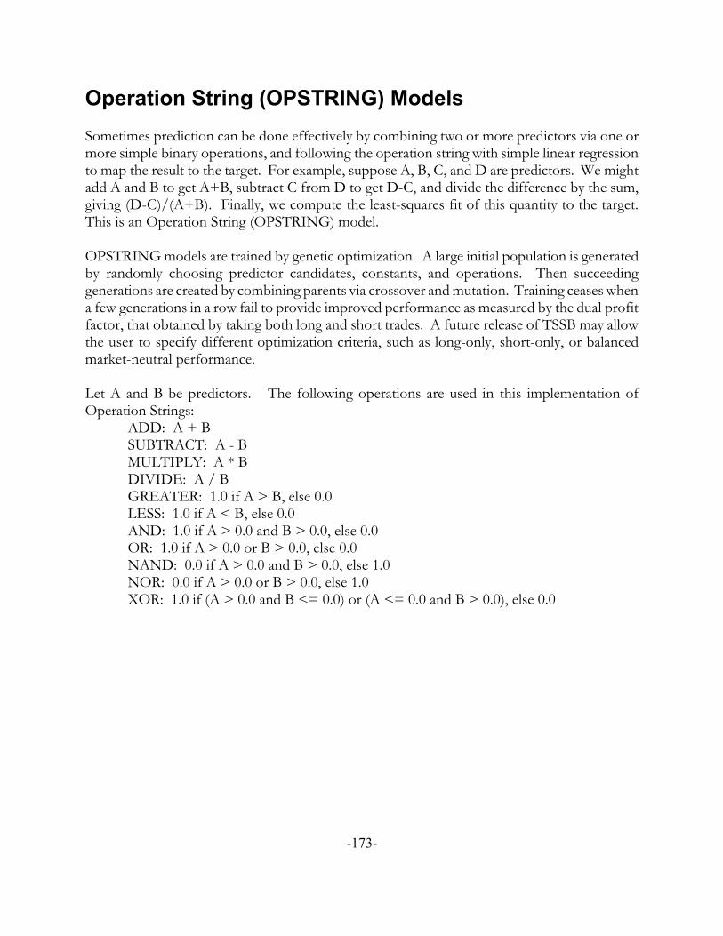
Operation String (OPSTRING) Models

Sometimes prediction can be done effectively by combining two or more predictors via one ormore simple binary operations, and following the operation string with simple linear regressionto map the result to the target. For example, suppose A, B, C, and D are predictors. We mightadd A and B to get A+B, subtract C from D to get D-C, and divide the difference by the sum,giving (D-C)/(A+B). Finally, we compute the least-squares fit of this quantity to the target. This is an Operation String (OPSTRING) model.

OPSTRING models are trained by genetic optimization. A large initial population is generatedby randomly choosing predictor candidates, constants, and operations. Then succeedinggenerations are created by combining parents via crossover and mutation. Training ceases whena few generations in a row fail to provide improved performance as measured by the dual profitfactor, that obtained by taking both long and short trades. A future release of TSSB may allowthe user to specify different optimization criteria, such as long-only, short-only, or balancedmarket-neutral performance.

Let A and B be predictors. The following operations are used in this implementation ofOperation Strings:

ADD: A + BSUBTRACT: A - BMULTIPLY: A * BDIVIDE: A / BGREATER: 1.0 if A > B, else 0.0LESS: 1.0 if A < B, else 0.0AND: 1.0 if A > 0.0 and B > 0.0, else 0.0OR: 1.0 if A > 0.0 or B > 0.0, else 0.0NAND: 0.0 if A > 0.0 and B > 0.0, else 1.0NOR: 0.0 if A > 0.0 or B > 0.0, else 1.0XOR: 1.0 if (A > 0.0 and B <= 0.0) or (A <= 0.0 and B > 0.0), else 0.0

-173-

In addition to the usual model options, the following items may (but do not have to) bespecified:

MAX LENGTH = IntegerThe maximum length of the operation string. Smaller values force simpler operations. The actual stringlength may be less than this quantity. This must be odd. (It will be decremented to an odd number ifspecified even.) The default is 7.

POPULATION = IntegerThe number of individuals in the population. Generally, this should be at least several times the numberof candidate predictors in order to provide sufficient genetic diversity. The default is 100.

CROSSOVER = RealNumberThis is the probability (0-1) of crossover. The default is 0.3.

MUTATION = RealNumberThis is the probability (0-1) of mutation. It should be small, because mutation is usually destructive. The default is 0.02.

REPEATS = IntegerIf this many generations in a row fail to improve the best child, training terminates. The default is 10.

CONSTANTS ( Probability ) = ListOfConstantsBy default, no constants are allowed in an operation string. This command lets the user request thatspecific constants or random constants within a range may be used. A range is specified by surroundinga pair of numbers with angle brackets, as in <-40 40>. The Probability (0-1) specifies the probabilitythat a constant will be used rather than a variable.

CONSTANTS IN COMPAREIf the user specifies a CONSTANTS list, then by default constants may be used in any operations. This option restricts constants to being used in compare operations (greater/less than).

CONSTANTS IN COMPARE TO VARIABLEThis is even more restrictive than the prior command. It restricts constants to use in comparisons tovariables.

-174-

LOGISTIC model considerations

Logistic regression is similar to linear regression. Its options are identical to those of a LINREGlinear regression model. However, some differences and special considerations are worthnoting:

! When the goal is to discriminate between two classes using some form of regression, onegenerally uses a target that is binary, either zero or one. In this case, logistic regressionis almost always much more robust against outliers in the predictors compared to linearregression. In short, when the goal is classification, logistic regression is nearly alwaysthe method of choice.

! The target must always be between zero and one, inclusive. Values outside this range willproduce nonsensical results. In most cases, the target will always be either zero (for oneclass) or one (for the other class). However, intermediate values are legal and may beused if the target genuinely asserts a probability of class membership.

! Because such targets are clearly not profits, it will virtually always be necessary to use thePROFIT= option to specify a profit variable for performance calculation.

! The output of the model is the estimated probability that the test case is a member of the‘one’ class.

Here is a sample logistic model application. Note how an expression transform is used to createthe binary target variable.

TRANSFORM BINOUT IS EXPRESSION (0) [ BINOUT = DAY_RETURN > 1.1 ] ;

MODEL MOD_LOG IS LOGISTIC [ INPUT = [ CMMA_5 LIN_5 RSI_5 ] OUTPUT = BINOUT PROFIT = DAY_RETURN MAX STEPWISE = 0 CRITERION = PROFIT FACTOR MIN CRITERION FRACTION = 0.1 ] ;

-175-

Regime Regression with SPLIT LINEAR Models

It is often the case that we cannot effectively model a process with a single model that isexpected to cover all states of the process. For example, one model may do a good job ofpredicting market movement when we are in a high-volatility regime, while a different modelmay be best in a low-volatility regime. These models may employ identical predictors but usethem differently. Or they may employ different predictors. A straightforward way ofperforming regime regression is with the SPLIT LINEAR model.

Selection of the predictors in a SPLIT LINEAR model takes place in two steps. The stepwiseprocess used for all models produces a pool of variables from which predictors for all regimeswill be chosen. At each step, the predictors in the current common pool will be optimallyassigned to the individual regime models.

In addition to selection of predictors, a gate variable will be chosen from a list supplied by theuser. An optimal split point (or two points) based on the gate variable will be computed in orderto define the regimes.

By default, every regime will have its own model. However, the SPLIT LINEAR SPLITS =NOISE option produces a different configuration. This option results in only one of tworegimes being modeled. The other regime is considered to be noise, and predictions madewithin this noise regime are always set equal to the training set target mean. As a result, tradeswill generally be rare within the noise regime.

-176-

The following options specially apply to SPLIT LINEAR models:

SPLIT VARIABLE = [ Var1 Var2 ... ]This lists one or more candidates for the variable that will define regimes. As in an INPUT list, arange may be specified with the dash (-).

SPLIT LINEAR SPLITS = IntegerThis specifies the number of split points, and it must be one or two. The number of regimes is one morethan the number of split points. If omitted, the default is 1.

SPLIT LINEAR SPLITS = NOISEThe domain is split into two regimes, but only one of the two regimes is modeled. The other regime isconsidered to be noise. Any prediction made within the noise regime will be set equal to the mean of thetarget variable within the training set. Note that it will not always be possible to meet the specifiedSPLIT LINEAR MINIMUM FRACTION specification when the NOISE option is invoked.

SPLIT LINEAR MAXIMUM INDICATORS = IntegerThis specifies the maximum number of predictors that will be used in each regime. These predictors willbe optimally chosen from the pool of candidates provided by the model’s stepwise selection process. If youwant to guarantee that the regimes can have completely disjoint predictor sets, the model’s MAXSTEPWISE must be equal to SPLIT LINEAR MAXIMUM INDICATORS times the numberof regimes. It makes no sense to make it larger. If omitted, the default is 2.

SPLIT LINEAR MINIMUM FRACTION = RealNumberThis specifies the minimum fraction of the training cases that must fall into each regime for the ordinaryversion of the model, and the minimum for the non-noise regime in the NOISE version. If the SPLITLINEAR SPLITS = NOISE option is used, it may not always be possible to satisfy this minimumfraction, especially if the value is 0.5 or greater. In this case, the program will come as close as it can. Also, note that if the NOISE option is not used, the maximum value for this MINIMUMFRACTION that the user may specify is 0.4. This ensures that degenerate conditions are avoided. Realize that in the ordinary version, a minimum exceeding 0.5 would be illegal because it is not possiblefor all regimes to contain more than half of the cases! If omitted, the default is 0.1.

SPLIT LINEAR RESOLUTION = IntegerThis is the number of split points that will be tested in order to define the regimes. Larger values requiremore run time but produce higher accuracy. If omitted, the default is 10. If there is one split point, thisquantity will determine how many splits are tested to find an approximate split, and then the exactoptimum will be found by further iterations. If there are two split points, no further refinement is done.

-177-

Input List Examples

Here are some examples of an input list:

INPUT = [ CMMA_5 CMMA_10 CMMA_20 ]These three variables are specified.

INPUT = [ CMMA_5 - CMMA_20 ]These two variables, as well as any that lie between them in the Variable List File, are specified.

INPUT = [ <NAME = “CLOSE MINUS MOVING AVERAGE” > ]All variables from this family are specified.

INPUT = [< NAME = “DELTA PRICE SKEWNESS” INDEX = MINUS >]All variables from the DELTA PRICE SKEWNESS family that are also of the MINUSINDEX version are specified.

INPUT = [< NAME = PRICE SKEWNESS >< NAME = CHANGE SKEWNESS >]All variables from the PRICE SKEWNESS as well as CHANGE SKEWNESS families arespecified.

-178-

Training and Testing Models

The following commands are available for training and testing models:

TRAIN ;All models are trained using all available cases in the database. Specifications of the model as well asits in-sample performance will be printed in both the AUDIT.LOG and REPORT.LOG files.

CROSS VALIDATE BY YEAR ;The model is cross validated using the year of each case as the fold variable. Specifications of each modelas well as its in-sample performance measures are printed to the AUDIT.LOG file but not theREPORT.LOG file. Out-of-sample results are printed to both files.

CROSS VALIDATE BY MONTH ;As above, except that hold-out blocks are one month long.

CROSS VALIDATE BY DAY ;As above, except that hold-out blocks are one day long.

CROSS VALIDATE BY VariableName ;As above, except that the named variable is used to control folds. Cases having exactly the same valueof this variable occupy the same fold.

CROSS VALIDATE BY VariableName ( Thresholds ) ;As above, except that folds are determined by where the value of the named variable lies among the oneor more specified thresholds. For example, suppose we have two thresholds: ( 0.3 0.7 ). Values lessthan 0.3 go into one fold. Values greater than or equal to 0.3 but less than 0.7 go into a second fold. Values of 0.7 or more go into the third fold. There will of course be one more fold than number ofthresholds.

CROSS VALIDATE Nfolds RANDOM BLOCKS ;As above, except that the specified number of folds are created by random selection of cases.

WALK FORWARD BY YEAR TrainYears StartYear ;The model is walked forward using the year of each case as the control variable. The user must specifythe number of years to include in each training period, and the starting year for testing. Specificationsof each model as well as its in-sample performance measures are printed to the AUDIT.LOG file butnot the REPORT.LOG file. Out-of-sample results are printed to both files.

WALK FORWARD BY MONTH TrainMonths StartDate ;As above, except that walking advances one month at a time. The start date must be expressed asYYYYMM.

-179-

WALK FORWARD BY DAY TrainDays StartDate ;As above, except that walking advances one day at a time. The start date must be expressed asYYYYMMDD.

Results include the number of cases tested and the number of those cases that equaled orexceeded the threshold. For criteria that are based on a threshold, the naive version of thecriterion is its value ignoring the model, using all cases in the fold. The thresholded version usesonly those cases whose predicted value meets the threshold.

If the user specified MCP TEST or a bootstrap test (Page 167 and following) in any modeldefinition, and if cross validation or walkforward testing is done, the test is performed on theout-of-sample results. This test computes the approximate probability that results as good asor better than those observed could have been obtained by pure luck from a worthless model.

When WALK FORWARD testing is done for a script file that includes one or more transforms,the transforms are evaluated for only the portion of the dataset needed at any time. This is thetraining set and the test set. The transform values are set to zero outside this area. Theimplication is that if prescreening is done based on a value produced by a transform, the numberof cases in the dataset passing the prescreen, a value reported in the audit log, may change as thewalkforward progresses. This is information only, and has no bearing on results.

-180-

Model Examples

Here is an example of a simple model definition and its evaluation. It should be self-explanatory.

MODEL mod1 IS LINREG [ INPUT = [ CMMA_5_S CMMA_5_N CMMA_5_S_C CMMA_5_N_C CMMA_50_S CMMA_50_N CMMA_50_S_C CMMA_50_N_C ] OUTPUT = LOGRET MAX STEPWISE = 3 CRITERION = PROFIT FACTOR MIN CRITERION CASES = 3000 RESTRAIN PREDICTED MCP TEST = 1000 ] ;CROSS VALIDATE BY YEAR ;

-181-

Committees

A committee is a lot like a model. In fact, the following MODEL options (see Page 160) canbe used in a committee:

INPUT =OUTPUT =PROFIT =LONG ONLYSHORT ONLYMAX STEPWISE =STEPWISE RETENTION =CRITERION =MIN CRITERION CASES =MIN CRITERION FRACTION =RESTRAIN PREDICTEDMCP TEST =

A committee is specified with the following command:

COMMITTEE CommName IS CommType [ CommSpecs ] ;

At this time, these committee types are available:AVERAGE - The output is the average (mean) of the inputsLINREG - Ordinary linear regression is used to model the targetCONSTRAINED - A linear combination constrained to positive weights that sum to

oneGRNN - General Regression Neural NetworkMLFN - Multiple-Layer Feedforward NetworkTREE - Simple binary treeFOREST - ForestBOOSTED TREE - Boosted tree

The greatest difference between a model and a committee is that a model’s input list (usually)names predictor variables, while a committee’s input list (always) names models. The namedmodel outputs are chosen by forward stepwise selection unless MAX STEPWISE is specifiedas zero, in which case all models are used.

-182-

OraclesAn oracle is an intelligent committee. Like a committee, it combines predictions from multiplemodels in order to produce a single consensus prediction. However, an oracle uses one or moregate variables to control the relative weighting of the component models. A committee uses asingle predefined methodology for all cases processed. An oracle changes its combining methodaccording to the value of the gate variable(s). This is extremely powerful, because it allowsdifferent models to be differently weighted in different conditions. For example, some modelsmight be favored in a high-volatility market, while others might dominate in a low-volatilitymarket.

The following MODEL options (see Page 160) can be used in an oracle:INPUT =OUTPUT =PROFIT =LONG ONLYSHORT ONLYCRITERION =MIN CRITERION CASES =MIN CRITERION FRACTION =RESTRAIN PREDICTEDMCP TEST =

Note that stepwise options are not allowed, because all component models are alwaysconsidered. The following options are specific to an oracle:

GATE = [ Var1 Var2 ... ] ;(Mandatory) This lists the variables that will be used as gates. It is strongly recommended that only onevariable be used. Training time and the risk of overfitting both explode if even two variables are used.

HONOR PRESCREEN ;(Optional) If one or more of the component models has a PRESCREEN (Page 161) that is also agate, and if this option is specified, training and execution of the oracle will, for any given case, consideronly models whose value of the gate variable lies within the prescreen range. If any component model hasa prescreen, it is almost always sensible (though not required) to make this prescreen a gate and specifythe HONOR PRESCREEN option.

An oracle is specified with the following command:

ORACLE OracleName [ CommSpecs ] ;

-183-

Oracles and Prescreening

There are two quite different philosophies for using an oracle. Neither is inherently superior tothe other. Different applications may favor different alternatives.

The simplest method is to train two or more models on the entire dataset, and intelligentlycombine their predictions based on values of a gate variable. The gate may be one of thepredictors, although this would almost never be the case. A model output cannot be used as agate. The component models would typically be different in fundamental design. For example,they may use different predictor sets, different targets, or different optimization criteria. Thekey is that they all share the same (complete) training set. Their differences come fromfundamental design changes.

An alternative oracle technique is to train specialist models via the PRESCREEN option (Page161) and use the oracle to oversee their decisions. For example, one might train three modelsbased on the value of a trend variable. One model might specialize in down markets, andsecond in flat markets, and the third in up markets. The oracle would use the prescreen variableas its gate. If the HONOR PRESCREEN option is specified for the oracle and a componentmodel’s prescreen variable is also a gate, training and execution cases will be processed for thecomponent model if and only if and the value of this variable is within the prescreen range ofthe model. Note that when a prescreened model is used in an oracle, in the vast majority ofapplications one should make the prescreen variable a gate and specify the HONORPRESCREEN option. Otherwise the model will be trained as a specialist, but the specializationwill be ignored when the model is used by the oracle. This is silly.

In a prescreened specialist situation, it is perfectly legal to use one or more gate variables thatare not prescreen variables (keeping in mind that the prescreen variables should also be gates!). Such a gate will impact all cases in all models. However, note that when more than one gate isemployed, training time may become excessive.

-184-

Here is an example of using three specialist models in conjunction with an oracle that combinesthem according to their specialization.

MODEL MOD_DOWN IS LINREG [ INPUT = [ X1 - X10 ] OUTPUT = DAY_RETURN PRESCREEN TREND < -10 MAX STEPWISE = 2 CRITERION = PROFIT FACTOR MIN CRITERION FRACTION = 0.1 ] ;

MODEL MOD_FLAT IS LINREG [ INPUT = [ X1 - X10 ] OUTPUT = DAY_RETURN PRESCREEN TREND > -10 PRESCREEN TREND < 10 MAX STEPWISE = 2 CRITERION = PROFIT FACTOR MIN CRITERION FRACTION = 0.1 ] ;

MODEL MOD_UP IS LINREG [ INPUT = [ X1 - X10 ] OUTPUT = DAY_RETURN PRESCREEN TREND > 10 MAX STEPWISE = 2 CRITERION = PROFIT FACTOR MIN CRITERION FRACTION = 0.1 ] ;

ORACLE ORACLE_TREND [ INPUT = [ MOD_DOWN MOD_FLAT MOD_UP ] OUTPUT = DAY_RETURN GATE = [ TREND ] HONOR PRESCREEN MIN CRITERION FRACTION = 0.1 ] ;

-185-

Trade FilteringIt is possible to read a file containing trade decisions produced by another program and then usethe TSSB program to attempt to improve performance by choosing to enhance or abort certaintrades. The format for reading a Haugen file is described on Page 11. Here, we describe howtrade filtering can be performed.

When a trade file is read, two new predictor variables will be automatically added to the variablelist. They may be plotted through the menu system, and one or both may optionally be placedin an INPUT list for a model. These variables are:

FILTER VALUE - This is the value of the variable that determines trades in the externalsystem. In the case of a Haugen file, this is his predicted alpha.

FILTER FRACTILE - For each date, the filter values are ranked across all markets that haverecords on this date. The market having minimum value will be given a fractile of -50. The largest will have a fractile of 50. Other markets will have equally spaced intermediatevalues.

Residuals

There are two main approaches to using models and committees to filter trades generated by anexternal system. One method is to use an actual future return as a target, and supply theFILTER VALUE and/or FILTER FRACTILE as supplementary inputs to a model or models. The idea is that the combination of the external prediction with TSSB variables will provesuperior to one or the other.

A frequently useful alternative is to compute the difference between the actual future return andthe prediction from the external model. This difference is called the residual, and it can be anexcellent prediction target. The idea is that if we can devise a means of estimating the externalsystem’s error, we can add our predicted error to the external system’s prediction in order togenerate a more accurate prediction of future return. Thresholds would be computed for thissum, rather than for the predicted residual itself.

Residual variables are computed by defining a target variable in the usual way, except that thekeyword RESIDUAL appears last on the definition line.

It is vital that the future variable and the external system’s prediction be measuring the samething in the same way, so that the difference between these two quantities measures only

-186-

prediction error of the external system. For example, if one of the quantities is annualized andthe other is not, the difference will be nearly meaningless.

Because of this rather stringent requirement of commensurability, it is usually best to performcross-market normalization on both variables. You need specify this only on the target variable. If done, the external system’s prediction is also cross-market normalized. For example, considerthis line in a definition file:

RESID_C: NEXT MONTH ATR RETURN 250 ! 0.3 RESIDUAL

For each date in the filter file, this will compute the NEXT MONTH ATR RETURN for allmarkets on that date, rank the returns for all markets, and compute the variable rescaled to arange of -50 (for the market having least return) to 50 (for the marking having maximum return). The external system’s predictions for all markets on that date will be similarly ranked. Then thedifference for each market will be computed as the predicted variable RESID_C. An implicationis that this variable will have theoretical limits of -100 to 100. Markets for which the actualreturn greatly exceeds the external system’s prediction will have a large value for this variable,while small values (very negative) will be obtained when the external system’s prediction greatlyexceeds the actual future return.

Note that if a residual variable is used as the model’s output, you must also supply a PROFITvariable (Page 16, 161) to use for computing profit-based performance measures. Residualsmake no sense as profits.

Committees, Oracles, and Trade Filtering

A committee or oracle can be used in trade filtering. As was the case with models, you caneither predict the actual future return, or you can predict the residual difference between thefuture return and the prediction made by the external system.

Because a committee attempts to combine multiple predictions of a quantity into a singlesuperior prediction, it is vital that the quantities being combined (the model outputs) all measurethe same thing. Thus it makes no sense to use a committee to combine the output of a modelpredicting a cross-sectionally normalized return with that of a model predicting an actual return. Also, it probably makes no sense to combine a one-day-ahead prediction with a one-month-ahead prediction.

Moreover, one cannot in principle combine a predicted residual with a predicted actual value,or use one of these as an input to a committee predicting the other. However, the TSSBprogram allows you do get away with this by performing an internal fix. If the committee ispredicting an actual value, and a component model is predicting a residual, the external system’s

-187-

prediction will be added to the model’s prediction before presentation to the committee. Similarly, if the committee is predicting a residual, and a component model is predicting anactual value, the external system’s prediction will be subtracted from the model’s predictionbefore presentation to the committee.

Comparing Our System with the External System

If the external system makes only binary trade decisions, it is perfectly reasonable to judge thequality of our system by comparing the profit factor of our system above its threshold with thatof all cases. If our system makes uselessly random predictions, these two profit factors will benearly equal. But if our system is good, the cases above (or below, for shorts) the threshold willhave a profit factor that exceeds that of the general population (the trades indicated by theexternal system).

However, if the external system makes continuous predictions, with the ultimate trade decisionsbeing based on the value of the prediction relative to a threshold determined by value orquantile, the comparison is not straightforward. Suppose that on each date we choose the topten percent of the external system’s predictions as our population, and we in turn decide to keepthe top ten percent of our predictions within that select population. Thus, we would beultimately be keeping one percent of the original system’s predictions (ten percent of tenpercent). It would not be fair to compare the performance of our top ten percent with that ofour population (the external system’s top ten percent). Rather, we would need to compare ourtop ten percent with the top one percent of the original system’s predictions.There is a reasonable way to make fair comparisons. For each date in the external system’sprediction database, we rank its predictions across all markets for which predictions were madeon that date. We similarly rank our predictions for that date. Then, for select fractiles, wecompare the profit factor of the filter’s predictions in that fractile with our model’s predictionsin the same fractile. The superior system will have greater profit factors across most or allfractiles.

A Useless but Instructive Script File

The following is one of the many script files that I used to verify (hopefully!) correct operationof the program. First, however, note the variable definition file that accompanies this script:

LIN_ATR_5: LINEAR PER ATR 5 100RETURN: NEXT MONTH ATR RETURN 250RETURN_CHEAT: NEXT MONTH ATR RETURN 250RESID: NEXT MONTH ATR RETURN 250 RESIDUAL

-188-

RESID_CHEAT: NEXT MONTH ATR RETURN 250 RESIDUALRETURN_C: NEXT MONTH ATR RETURN 250 ! 0.3RETURN_C_CHEAT: NEXT MONTH ATR RETURN 250 ! 0.3RESID_C: NEXT MONTH ATR RETURN 250 ! 0.3 RESIDUALRESID_C_CHEAT: NEXT MONTH ATR RETURN 250 ! 0.3 RESIDUAL

Observe that every target variable appears twice, once with a descriptive name and again withthe same name followed by CHEAT. This lets us train perfect models. The main models in thisscript file use the same predictor and target. The idea is that all results should be perfect to theextent that is theoretically possible. My hope is that any bugs in the program will manifestthemselves as less-than-perfect results for this script.

This script appears here because it is instructive in that it demonstrates the many ways we cantrain models and committees in the task of filtering an existing trading system. The commentsinserted in the listing should explain its operation.

-189-

//*****************************************************************************// This script file demonstrates the wide variety of possibilities in// filtering an external model.// In all cases, appending _C to a model or variable means that it uses// cross-sectionally normalized values.// Appending _CHEAT to a variable name means that it is just another name// for the same variable. This lets us create perfect models.//*****************************************************************************

//*****************************************************************************// Models DUMMY and DUMMY_C are deliberately weak models intended only to// serve as 'second models' in committees, where they will be rejected.//*****************************************************************************

MODEL DUMMY IS LINREG [ INPUT = [ LIN_ATR_5 ] OUTPUT = RETURN MAX STEPWISE = 1 CRITERION = PROFIT FACTOR MIN CRITERION FRACTION = 0.1 MCP TEST = 100 ] ;

MODEL DUMMY_C IS LINREG [ INPUT = [ LIN_ATR_5 ] OUTPUT = RETURN_C MAX STEPWISE = 1 CRITERION = PROFIT FACTOR MIN CRITERION FRACTION = 0.1 MCP TEST = 100 ] ;

-190-

//*****************************************************************************// Model TWEAK is a simple model that predicts actual return using itself.// Naturally, it will do a perfect job!//*****************************************************************************

MODEL TWEAK IS LINREG [ INPUT = [ RETURN_CHEAT ] OUTPUT = RETURN MAX STEPWISE = 1 CRITERION = PROFIT FACTOR MIN CRITERION FRACTION = 0.1 MCP TEST = 100 ] ;

//*****************************************************************************// This model does the same thing, except that the predicted value (as well// as the identical predictor) are cross-sectionally normalized.// Since the predictor and predicted are the same values, we would expect// perfection. And we get it in MSE and R-Square.// But profit factors are not perfect, just excellent. Why?// We would get perfect profit factors if the ranking were done across the// entire dataset. But we don't. We normalize separately for each day.// Some days are overall up, and others down. So some days a high rank may// still correspond to a loss, and other days a low rank may still be a win.//*****************************************************************************

MODEL TWEAK_C IS LINREG [ INPUT = [ RETURN_C_CHEAT ] OUTPUT = RETURN_C PROFIT = RETURN MAX STEPWISE = 1 CRITERION = PROFIT FACTOR MIN CRITERION FRACTION = 0.1 MCP TEST = 100 ] ;

-191-

//*****************************************************************************// This model predicts the residual, the actual return minus the FILTER_VALUE.// When thresholds are computed, the FILTER_VALUE is added to the prediction// to get the value that is thresholded.//*****************************************************************************

MODEL RESIDUAL IS LINREG [ INPUT = [ RESID_CHEAT ] OUTPUT = RESID PROFIT = RETURN MAX STEPWISE = 1 CRITERION = PROFIT FACTOR MIN CRITERION FRACTION = 0.1 MCP TEST = 100 ] ;

//*****************************************************************************// This is identical to the prior model except that the predicted value is// the cross-sectional rank of the actual return minus the cross-sectional// rank of the FILTER_VALUE, which is known as FILTER_FRACTILE.//*****************************************************************************

MODEL RESIDUAL_C IS LINREG [ INPUT = [ RESID_C_CHEAT ] OUTPUT = RESID_C PROFIT = RETURN MAX STEPWISE = 1 CRITERION = PROFIT FACTOR MIN CRITERION FRACTION = 0.1 MCP TEST = 100 ] ;

-192-

//*****************************************************************************// This is a simple committee.// It predicts actual return from the output of a model that also predicts// actual return.//*****************************************************************************

COMMITTEE HYBRID1 IS AVERAGE [ INPUT = [ TWEAK DUMMY ] OUTPUT = RETURN MAX STEPWISE = 1 CRITERION = PROFIT FACTOR MIN CRITERION FRACTION = 0.1 MCP TEST = 100 ] ;

//*****************************************************************************// This is a more complex committee. It predicts the residual by using the// output of a model that predicts actual values. Thus, before the model's// output is presented to the committee, it is reduced by FILTER_VALUE.// After the committee makes its prediction, FILTER_VALUE is added back// to the prediction prior to computing or using a threshold.//*****************************************************************************

COMMITTEE HYBRID2 IS AVERAGE [ INPUT = [ TWEAK DUMMY ] OUTPUT = RESID PROFIT = RETURN MAX STEPWISE = 1 CRITERION = PROFIT FACTOR MIN CRITERION FRACTION = 0.1 MCP TEST = 100 ] ;

-193-

//*****************************************************************************// This is the opposite of the prior committee.// It predicts an actual return using the output of a model that predicts// the residual. Thus, before the output of the model is presented to the// committee, FILTER_VALUE is added to it.//*****************************************************************************

COMMITTEE HYBRID3 IS AVERAGE [ INPUT = [ RESIDUAL DUMMY ] OUTPUT = RETURN MAX STEPWISE = 1 CRITERION = PROFIT FACTOR MIN CRITERION FRACTION = 0.1 MCP TEST = 100 ] ;

//*****************************************************************************// This is a consistent model in that it predicts the residual using the// output of a model that also predicts the residual. Thus, the model's// output is presented to the committee unchanged. The committee's output// is increased by FILTER_VALUE before thresholds are computed or used.//*****************************************************************************

COMMITTEE HYBRID4 IS AVERAGE [ INPUT = [ RESIDUAL DUMMY ] OUTPUT = RESID PROFIT = RETURN MAX STEPWISE = 1 CRITERION = PROFIT FACTOR MIN CRITERION FRACTION = 0.1 MCP TEST = 100 ] ;

-194-

//*****************************************************************************// These four committees are identical to the prior four except that they// work with cross-sectionally normalized values instead of actual values.//*****************************************************************************

COMMITTEE HYBRID1_C IS AVERAGE [ INPUT = [ TWEAK_C DUMMY_C ] OUTPUT = RETURN_C PROFIT = RETURN MAX STEPWISE = 1 CRITERION = PROFIT FACTOR MIN CRITERION FRACTION = 0.1 MCP TEST = 100 ] ;

COMMITTEE HYBRID2_C IS AVERAGE [ INPUT = [ TWEAK_C DUMMY_C ] OUTPUT = RESID_C PROFIT = RETURN MAX STEPWISE = 1 CRITERION = PROFIT FACTOR MIN CRITERION FRACTION = 0.1 MCP TEST = 100 ] ;

COMMITTEE HYBRID3_C IS AVERAGE [ INPUT = [ RESIDUAL_C DUMMY_C ] OUTPUT = RETURN_C PROFIT = RETURN MAX STEPWISE = 1 CRITERION = PROFIT FACTOR MIN CRITERION FRACTION = 0.1 MCP TEST = 100 ] ;

-195-

COMMITTEE HYBRID4_C IS AVERAGE [ INPUT = [ RESIDUAL_C DUMMY_C ] OUTPUT = RESID_C PROFIT = RETURN MAX STEPWISE = 1 CRITERION = PROFIT FACTOR MIN CRITERION FRACTION = 0.1 MCP TEST = 100 ] ;

-196-

Miscellaneous CommandsThis section discusses commands that do not readily fit into any other category.

Clumped trades

Some analysts evaluate the performance of a trading system by calculating trade profits from theopening of the trade to the closing of the trade. Others, including myself, prefer to markpositions to market every day (or bar if intraday). This is done for nearly all profit calculationsin this program. This fine granularity is especially important for profit factor calculations. Thefollowing commands can be used to combine a position vector with a return vector andcompute some statistics based on clumped trades (trades defined as open-to-close of position).

CLUMPED PROFIT FACTOR PosVar RetVar ;CLUMPED PROFIT FACTOR PosVar RetVar MCreps ;

The position vector must be integers, typical zero and plus or minus one. If MCreps is specified,crude Monte-Carlo tests are performed by shuffling and rotating the returns.

-197-

Chi-Square Tests

It can be interesting to test a set of individual predictor candidates to discover the degree towhich they are related to a target. The following command does this in the most basic version. Several variations are available and will be described later. A mouse-based GUI interface is alsoavailable and will be discussed later.

CHI SQUARE [Pred1 Pred2 ...] (Nbins) WITH Target (Nbins) ;

The user specifies a list of predictor candidates, the number of bins for predictors (at least 2),a single target, and the number of bins for this target (at least 2).

The program will print to AUDIT.LOG a list of the predictor candidates, sorted from maximumrelationship (Cramer’s V) to minimum. In addition to printing the chi-square value, it will alsoprint the contingency coefficient, Cramer’s V, and a p-value.

The contingency coefficient is a nominal form of correlation coefficient. Note, however, thatunlike ordinary correlation, its maximum value is less than one. If the table is square with k binsin each dimension, the maximum value of the contingency coefficient is sqrt ((k-1)/k).

Cramer’s V is a slightly better nominal correlation coefficient. It ranges from zero (norelationship) to one (perfect relationship).

The p-value does not take into account the fact that we are doing multiple tests. It is the p-valueassociated with a single test of the given predictor with the target. An option for taking selectionbias (choosing the best indicators from a set of many candidates) into account will be discussedlater.

The advantage of a chi-square test over ordinary correlation is that it is sensitive to nonlinearrelationships. An interaction that results in certain regions of the predictor being associated withunexpected values of the target can be detected.

Larger numbers of bins increase the sensitivity of the test because more subtle relationships canbe detected. However, p-values become less reliable when bin counts are small. As a generalrule of thumb, most cells should have an expected frequency of at least five, and no cell shouldhave an expected frequency less than one. But keep in mind that because we are doing multiplecomparisons, individual p-values don’t mean much anyway. The primary value of this test is theordering of predictor candidates from maximum target relationship to minimum.

-198-

Options for the Chi-Square Test

The prior section discussed the most basic version of the chi-square test. Any or all of severaloptions may be added to the command to extend the test. Suppose we have the following basicchi-square test:

CHI SQUARE [ X1 X2 X3 ] ( 3 ) WITH RET ( 3 ) ;

The test shown above splits each indicator candidate (X1, X2, X3) into three equal bins, and itdoes the same for the target, RET. We can replace the number of bins for the indicators witha fraction ranging from 0.0 to 0.5 (typically 0.05 or 0.1) and the word TAILS to specify that thetest employ just two bins for the indicator, the most extreme values. The following commandsays that cases with indicator values in the highest 0.1 (ten percent) of all cases go into one bin,cases whose indicator is in the lowest 0.1 go into the other bin, and the 80 percent middle valuesof the indicator will be ignored.

CHI SQUARE [ X1 X2 X3 ] 0.1 TAILS WITH RET ;

Another option is to specify that instead of using equal-count bins for the target, the sign of thetarget (win/loss) is used. This implies that there are only two target bins: win and lose. (Notethat using three bins is often better than splitting at zero, because this splits the target into bigwin, big loss, and near zero.) We split at zero by replacing the bin count with the word SIGN. The following command does this:

CHI SQUARE [ X1 X2 X3 ] ( 3 ) WITH RET SIGN ;

Finally, it was already mentioned that the p-values printed with the basic test are individual,appropriate only if you test exactly one indicator. When you test many indicators and look forthe best, lucky indicators will be favored. This is called selection bias, and it can be severe,causing huge underestimation of the correct p-value. A Monte-Carlo Permutation Test (MCPT)can be employed to approximately control for selection bias. This is done by appending MCPT= Nreps at the end of the command, as is shown in the following example. Note that if thetarget has significant serial correlation, as would be for look-aheads more than one bar, thecomputed p-value will be biased downward.

CHI SQUARE [ X1 X2 X3 ] ( 3 ) WITH RET ( 3 ) MCPT=100 ;

Finally, we can combine any or all of these options as shown below:

CHI SQUARE [ X1 X2 X3 ] 0.1 TAILS WITH RET SIGN MCPT=100 ;

See Running Chi-Square Tests from the Menu on Page 202, 208 for more discussion of these options.

-199-

Output of the Chi-Square Test

The following table is a typical output from the chi-square test:

Chi-square test between predictors (2 bins) and DAY_RETURN_1 (3 bins) (Sorted by Cramer's V) Tails only, each tail fraction = 0.050

Variable Chi-Square Contingency Cramer's V Solo pval Unbiased p

INT_5 30.02 0.225 0.231 0.0000 0.0010DPPV_10 13.43 0.152 0.154 0.0012 0.2370DINT_10 12.70 0.148 0.150 0.0017 0.3270PENT_2 10.59 0.104 0.105 0.0050 1.0000

The heading for this table shows that two bins were used for the predictor (indicator here,though it can be interesting to use targets as predictors!) and three for the target. Only the tailswere used for the predictors, the upper and lower five percent.

The indicators are listed in descending order of Cramer’s V. This is a better quantity to sort thaneither chi-square or the contingency coefficient, because it is the best at measuring the practicalrelationship between the indicator and the target. Chi-square and the contingency coefficientare especially problematic for sorting when the indicator contains numerous ties. Also, the real-life meaning of chi-square and the contingency coefficient is vague, while Cramer’s V is easilyinterpretable because it lies in the range of zero (no relationship) to one (perfect relationship).

The solo pval column is the probability associated with the indicator’s chi-square, when thatindicator is tested in isolation. This would be a valid p-value to examine if the user picked a singleindicator in advance of the test. But because we will typically be examining a (frequently large)collection of candidate indicators, and focusing on only the best from among them, there is ahigh probability that indicators that were simply lucky hold our attention. Their luck willproduce a highly significant (very small) p-value and we will be fooled. Thus, it is important thatwe compensate for the impact of luck. Also note that the solo p-value, like nearly all teststatistics, assumes that the cases are independent. This assumption will be violated if the targetlooks ahead more than one bar.

A Monte-Carlo Permutation Test with 1000 replications was performed, and its results areshown in the last column labeled ‘unbiased pval’. The smallest p-value possible is the reciprocalof the number of replications, so the minimum here is 0.001. This unbiased p-value will becorrect (within the limitations of a MCPT) for only the indicator having largest Cramer’s V. Allothers will somewhat over-estimate the correct p-value. But that’s fine, because we at least knowthat the true p-value does not exceed that shown. There does not appear to be any way to

-200-

compute MCPT p-values that are correct for all indicators. Also, the MCPT p-values will bebiased downward if the target looks ahead more than one day.

The most important thing to note is that for targets that have little or no serial correlation, theunbiased p-value, which takes selection bias into account, can (and usually does) greatly exceedthe solo p-value.

It the user specified that the predictors are to be tails only, the table shown above is followedby a smaller table showing the value of the lower and upper tail thresholds. This table looks likethe following:

Variable Lower thresh Upper threshCMMA_20 -31.6299 35.5345CMMA_5 -35.1684 37.1704

-201-

Figure 12: Dialog box for chi-square tests

Running Chi-Square Tests from the Menu

As an alternative to issuing commands in a script file, chi-square tests can be run from the menuby clicking Describe / Chi-Square. The following dialog box will appear:

The user selects one or more predictors (usually indicators, but target variabless can be selectedas well) from the left-hand list. Selection can be done in any of three ways:

1) Drag across a range of predictors to select all of them.

2) Select a predictor, hold down the Shift key, and select another predictor to select all predictorsthat lie between them.

3) Hold the Ctrl key while clicking any predictor to toggle it between selected and not selected,without impacting existing selections.

A single target must be selected.

-202-

The user must specify how the predictor bins are defined. There are two choices:

1) Select ‘Use all cases’ and enter the number of equal-count bins to employ.

2) Select ‘Use tails only’ and enter the tail fraction on each side (greater than zero and less than0.5) to employ two bins, one for each tail, with interior values ignored. Values of 0.05 or 0.1 aretypical. Keeping more than ten percent of each tail usually results in significant loss of predictivepower. The majority of predictive power in most indicators lies in the most extreme values.

The user must specify how the target bins are defined. There are two choices:

1) Select ‘Split equally’ and specify the number of equal-count bins to employ. In most cases thisis the best choice, with three bins used. Three equal-count bins split the target into ‘big win’,‘big loss’, and ‘fairly inconsequential’ trade outcomes. (This labeling assumes that the targetdistribution is fairly symmetric, the usual situation.)

2) Select ‘Split at Zero’, in which case there are two bins, with bin membership defined by thesign of the target. A target value of zero is considered to be a win.

Note that if the user selects ‘Use tails only’ for the predictor and ‘Split equally’ for the target, thetarget bin thresholds are defined by the entire target distribution, not the distribution in thepredictor tails only. In most cases this results in a more sensitive test than determining the splitpoints using predictor tails only.

Finally, the user can specify ‘Permutation replications’ to be a number greater than zero in orderto perform a Monte-Carlo Permutation Test of the null hypothesis that all predictors areworthless for predicting the target (at least in terms of the chi-square test performed). If this isdone, at least 100 replications should be used, and 1000 is not unreasonable. The smallestcomputed p-value possible is the reciprocal of the number of replications. The MCPT willproduce a column labeled ‘Unbiased p’ which contains an upper bound (exact for the firstpredictor listed, increasingly conservative for subsequent predictors) on the probability that aset of entirely worthless predictors could have produced a best predictor as effective as the oneobserved. It would be nice to have exact unbiased p-values for predictors below the first (best),but there does not appear to be a practical way of computing this figure. Still, having the p-values be conservative (too large) is better than having them anti-conservative (too small). Atleast you know that the true p-value is no worse than that shown for each predictor. But notethat if the target has significant serial correlation, as would be for look-aheads more than onebar, the computed p-value will be biased downward.

-203-

Nonredundant Predictor Screening

The chi-square test described in the prior section is an effective way to rapidly screen a set ofcandidate indicators and rank them according to their power to predict a target variable. However, it has one disadvantage: indicators can be seriously redundant. This is especially truein regard to the information in the indicators which is related to the target. A statistical studyof indicators alone (ignoring a target) may show that they have little correlation. However, if onedevises a test which considers only that information component of the indicators that is relatedto a target variable, the degree of redundancy of this predictive information can be high. Thuswe are inspired to consider an alternative test.

The method employed in TSSB operates by first selecting from a list of candidates the indicatorthat has the most predictive power. Then the candidate list is searched to find the indicatorwhich adds the most predictive power to that obtained from the first selection. When a secondindicator has been found, a third is chosen such that it adds the most predictive power to thatalready obtained from the first two. This repeats as desired.

The algorithm just described is in essence ordinary stepwise selection, similar to that obtainablefrom building predictive models. However, it is different in several ways:

! Because the algorithm is based on segregating the data into bins, it can detect nonlinearrelationships without imposing the restrictions of a formally defined model.

! Unlike the models in TSSB (and those available in any other statistics packages knownto the author), this algorithm allows the option of examining only extreme values of thecandidate indicators. It is well known that in most situations, the majority of usefulpredictive information is found in the tails of indicators.

! The relative simplicity and speed of this algorithm makes it possible to perform Monte-Carlo Permutation Tests of the indicator sets to help decide which predictors and setshave legitimate predictive power and which were just lucky.

The following command does this in the most basic version. Note that it is identical to thesyntax of the chi-square test of the prior section, except for the beginning of the command. Several variations are available and will be described later. A mouse-based GUI interface is alsoavailable and will be discussed later.

NONREDUNDANT PREDICTOR SCREENING[Pred1 Pred2 ...] (Nbins) WITH Target (Nbins) ;

-204-

The user specifies a list of predictor candidates, the number of bins for predictors (at least 2),a single target, and the number of bins for this target (at least 2).

The program will print to AUDIT.LOG a list of the predictor candidates, sorted into the orderin which the predictors were selected. This order can be interpreted as saying that the firstpredictor listed is the single most important, the second predictor is the one that contributed themost additional predictive information, and so forth.

Several columns of useful data are printed. These are:

Me an Co u n t is the mean number of cases expected in each cell. This is the total number ofcases going into the test, divided by the number of cells. The number of cells for the first (best)predictor is the number of predictor bins times the number of target bins. As each additionalpredictor is added to the set, the number of cells is multiplied by the number of predictor bins. Obviously, if numerous predictor bins are specified, the number of cells will increase rapidly,and hence the mean per-cell count will drop rapidly. Larger counts produce a better test. If thecount drops below five, a warning message will be printed.

100*V is a nominal (category-based) correlation coefficient. It ranges from zero (norelationship) to 100 (perfect relationship). The primary disadvantage of Cramer’s V is that it issymmetric: the ability of the target to predict the predictor is given the same weight as the abilityof the predictor to predict the target. This is, of course, counterproductive in financialprediction.

100*Lam b d a is another nominal measure of predictive power which ranges from zero (norelationship) to 100 (perfect relationship). Unlike Cramer’s V, it is one-sided: it measures onlythe ability of the predictor to predict the target. Also unlike Cramer’s V, it is proportional in thesense that a value which is twice another value can be interpreted as implying twice thepredictive power. However, it has the property that it is based on only the most heavilypopulated cells, those that occur most frequently. If more thinly populated cells are just noise,this can be good. But in most cases it is best to consider all cells in computing predictive power.

100*URe d u c is an excellent measure of predictive power which is based on information theory. The label UReduc employed in the table is an abbreviation of Uncertainty Reduction. If nothing isknown about any predictors, there is a certain amount of uncertainty about the likely values ofthe target. But if a predictor has predictive power, knowledge of the value of this predictor willreduce our uncertainty about the target. The Uncertainty Reduction is the amount by which ouruncertainty about the target is reduced by gaining knowledge of the value of the predictor. Thismeasure is excellent. Like Lambda, it is one-sided, as well as proportional. But like Cramer’sV and unlike Lambda, it is based on all cells, not just those most heavily populated. So it hasall of the advantages and none of the disadvantages of the other two measures.

-205-

In c p v al is printed if the user specified that a Monte-Carlo Permutation Test be performed. Foreach predictor, this p-value is the probability that, if the predictor truly has no predictive powerbeyond that already contained in the predictors selected so far, we could observe an improvement at leastas great as that obtained by including this new predictor. A very small p-value indicates that thepredictor is effective at adding predictive power to that already available. Note that if the targethas significant serial correlation, as would be for look-aheads more than one bar, the computedp-value will be biased downward.

Grp p v al is printed if the user specified that a Monte-Carlo Permutation Test be performed. For each predictor, this p-value is the probability that, if the set of predictors found so far(including this one) truly has no predictive power, we could observe a performance at least asgreat as that obtained by including this new predictor. A very small p-value indicates that thepredictor set to this point is effective. Note that if the target has significant serial correlation,as would be for look-aheads more than one bar, the computed p-value will be biased downward.

The essential difference between these two p-values is that the inclusion p-value refers topredictive power gained by adding the predictor to the set so far, while the group p-value refers to thepredictive power of the entire set of predictors found so far.

The pattern of these p-values can reveal useful information. Suppose a very few predictors havegreat predictive power and the remaining candidates have none. The inclusion p-values for thepowerful predictors will be tiny, and the inclusion p-values for the other candidates will tend tobe larger, thus distinguishing the quality. But the group p-values will be tiny for all candidates,even the worthless ones, because the power of the effective few carries the group.

Now suppose that a few candidates have slight power, and the others are worthless. As in theprior example, the inclusion p-values for the effective candidates will be tiny, and the inclusionp-values for the other will tend to be larger. But the group p-value will behave differently. Asthe slightly effective predictors are added to the set, the group-p-value will tend to drop,indicating the increasing power of the group. But then as worthless candidates are added, thegroup p-value will tend to rise, indicating that overfitting is overcoming the weak predictors.

Remember, though, that when the mean case count per cell drops too low (indicated by a dashedline and warning), the behavior just discussed can change in random and meaningless ways.

By default, Uncertainty reduction is used for sorting the selected predictors and for the optional p-value computation. Also by default, the maximum number of predictors is fixed at eight, whichis nearly always more than enough. Neither of these defaults can be changed when this test isexecuted from within a script file, although this should not be a problem because they areexcellent choices. They can be changed by the user if this test is performed via the menu system,as discussed later.

-206-

Options for Nonredundant Predictor Screening

The options for nonredundant predictor screening are identical to those for the chi-square testdescribed in a prior section. Nevertheless, they will be repeated here for the reader’sconvenience, and expanded upon later. Suppose we have the following basic test:

NONREDUNDANT PREDICTOR SCREENING[ X1 X2 X3 ] ( 3 ) WITH RET ( 3 ) ;

The test shown above splits each indicator candidate (X1, X2, X3) into three equal bins, and itdoes the same for the target, RET. We can replace the number of bins for the indicators witha fraction ranging from 0.0 to 0.5 (typically 0.05 or 0.1) and the word TAILS to specify that thetest employ just two bins for the predictor, the most extreme values. The following commandsays that cases with indicator values in the highest 0.1 (ten percent) of all cases go into one bin,cases whose indicator is in the lowest 0.1 go into the other bin, and the 80 percent middle valuesof the indicator will be ignored.

NONREDUNDANT PREDICTOR SCREENING[ X1 X2 X3 ] 0.1 TAILS WITH RET ;

Another option is to specify that instead of using equal-count bins for the target, the sign of thetarget (win/loss) is used by splitting the bins at zero. This implies that there are only two targetbins: win and lose. (Note that using three bins is often better than splitting at zero, because thissplits the target into big win, big loss, and near zero.) We split at zero by replacing the bin countwith the word SIGN. The following command does this:

NONREDUNDANT PREDICTOR SCREENING[ X1 X2 X3 ] ( 3 ) WITH RET SIGN ;

It was already mentioned that p-values can be computed. When you test many predictors andrepeatedly look for the best to add, lucky predictors will be favored. This is called selection bias,and it can be severe, causing worthless predictors to be selected. A Monte-Carlo PermutationTest (MCPT) can be employed to approximately control for selection bias. This is done byappending MCPT = Nreps at the end of the command, as is shown in the following example:

NONREDUNDANT PREDICTOR SCREENING[ X1 X2 X3 ] ( 3 ) WITH RET ( 3 ) MCPT=100 ;

Finally, we can combine any or all of these options as shown below:

NONREDUNDANT PREDICTOR SCREENING[ X1 X2 X3 ] 0.1 TAILS WITH RET SIGN MCPT=100 ;

-207-

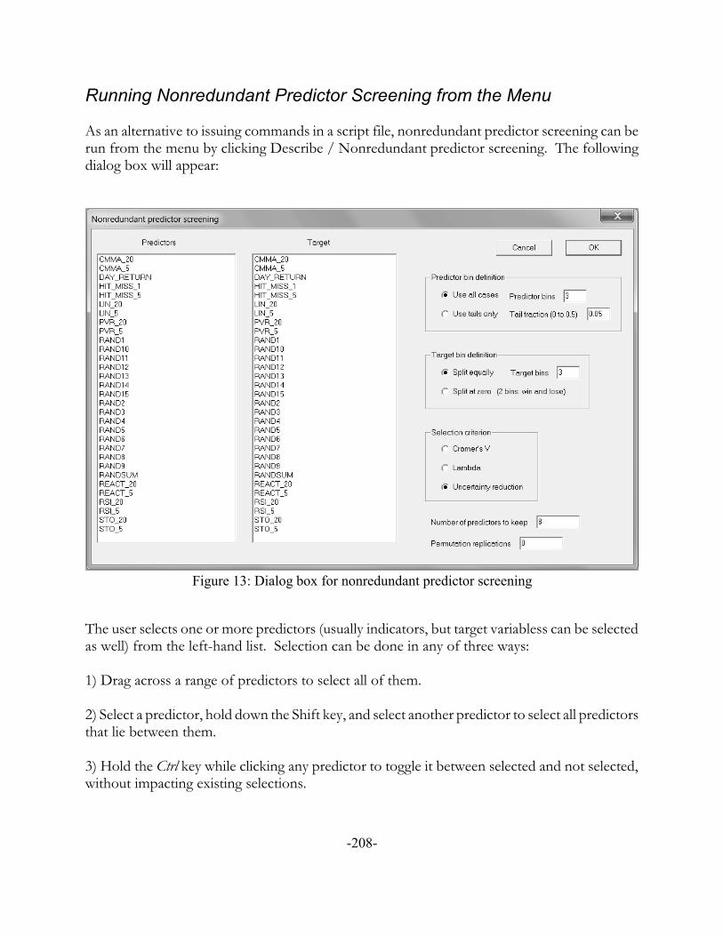
Figure 13: Dialog box for nonredundant predictor screening

Running Nonredundant Predictor Screening from the Menu

As an alternative to issuing commands in a script file, nonredundant predictor screening can berun from the menu by clicking Describe / Nonredundant predictor screening. The followingdialog box will appear:

The user selects one or more predictors (usually indicators, but target variabless can be selectedas well) from the left-hand list. Selection can be done in any of three ways:

1) Drag across a range of predictors to select all of them.

2) Select a predictor, hold down the Shift key, and select another predictor to select all predictorsthat lie between them.

3) Hold the Ctrl key while clicking any predictor to toggle it between selected and not selected,without impacting existing selections.

-208-

A single target must be selected.

The user must specify how the predictor bins are defined. There are two choices:

1) Select ‘Use all cases’ and enter the number of equal-count bins to employ.

2) Select ‘Use tails only’ and enter the tail fraction on each side (greater than zero and less than0.5) to employ two bins, one for each tail, with interior values ignored. Values of 0.05 or 0.1 aretypical. Keeping too little of each tail usually results in such rapid reduction in the mean per-cellcount that very few predictors can be safely selected.

The user must specify how the target bins are defined. There are two choices:

1) Select ‘Split equally’ and specify the number of equal-count bins to employ. In most cases thisis the best choice, with three bins used. Three equal-count bins split the target into ‘big win’,‘big loss’, and ‘fairly inconsequential’ trade outcomes. (This labeling assumes that the targetdistribution is fairly symmetric, the usual situation.)

2) Select ‘Split at Zero’, in which case there are two bins, with bin membership defined by thesign (win/lose) of the target. A target value of zero is considered to be a win.

Note that if the user selects ‘Use tails only’ for the predictor and ‘Split equally’ for the target, thetarget bin thresholds are defined by the entire target distribution, not the distribution in thepredictor tails only. In most cases this results in a more sensitive test than determining the splitpoints using predictor tails only.

The user may select which of the three available measures of predictive power is to be used forpredictor selection and optional Monte-Carlo Permutation Tests. The default, Uncertaintyreduction, is almost always far superior to the two alternatives, so it should be chosen unless theuser wishes to experiment.

The number of predictors to keep defaults to 8. In nearly all cases this is more than enough, ascell count reduction will render the tests meaningless before even 8 are reached, unless therehappens to be a huge number of history cases available. The user may set this to any desiredquantity. For example, if extensive history of many markets is in the database, increasing thisabove 8 may be appropriate. The only advantage to specifying a smaller number to keep is thatsmaller numbers kept will speed a Monte-Carlo Permutation Test.

Finally, the user can specify ‘Permutation replications’ to be a number greater than one in orderto perform a Monte-Carlo Permutation Test. If this is done, at least 100 replications should beused, and 1000 is not unreasonable. The smallest computed p-value possible is the reciprocalof the number of replications. The MCPT will produce a column labeled ‘Inclusion p-value’

-209-

which contains the probability that, if the predictor truly has no predictive power beyond thatalready contained in the predictors selected so far, we could observe an improvement at least asgreat as that obtained by including this new predictor. A very small p-value indicates that thepredictor is effective. Note that if the target has significant serial correlation, as would be forlook-aheads more than one bar, the computed p-value will be biased downward.

-210-

Examples of Nonredundant Predictor Screening

We end this discussion with a few progressive examples of nonredundant predictor screening. First, we’ll explore how the algorithm behaves in a simple contrived application. We generatea set of random numbers by means of the following commands:

TRANSFORM RAND1 IS RANDOM ;TRANSFORM RAND2 IS RANDOM ;TRANSFORM RAND3 IS RANDOM ;TRANSFORM RAND4 IS RANDOM ;TRANSFORM RAND5 IS RANDOM ;TRANSFORM RAND6 IS RANDOM ;TRANSFORM RAND7 IS RANDOM ;TRANSFORM RAND8 IS RANDOM ;

TRANSFORM RAND_SUM IS EXPRESSION (0) [ RAND_SUM = RAND1 + RAND2 + RAND3 + RAND4 + RAND5 ] ;

TRAIN ;

The commands just shown generate eight different random series, and then it creates a newseries RAND_SUM by summing the first five of these eight random series. Note that theTRAIN command is required because transforms are not computed until they are needed, suchas for training, walkforward testing, or cross validation.

Now suppose the following nonredundant predictor screening command appears:

NONREDUNDANT PREDICTOR SCREENING[ RAND1 RAND2 RAND3 RAND4 RAND5 RAND6 RAND7 RAND8 ](2)WITH RAND_SUM (2) MCPT=1000 ;

This command says that we will test all eight random series as predictors of a target whichconsists of the sum of the first five of the predictors. Two bins will be used for the predictors,and two for the target. A Monte-Carlo Permutation Test having 1000 replications will beperformed. Because we have contrived this test, we know that we can expect RAND1 throughRAND5 to be selected, and the others rejected.

-211-

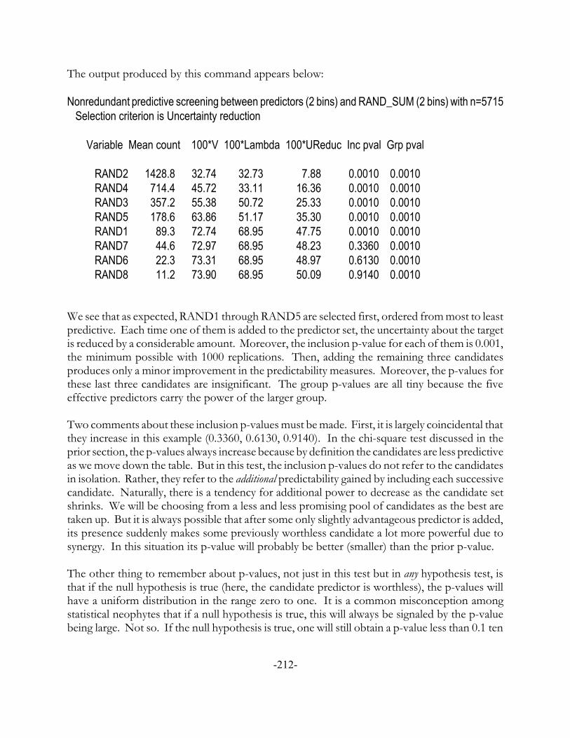
The output produced by this command appears below:

Nonredundant predictive screening between predictors (2 bins) and RAND_SUM (2 bins) with n=5715 Selection criterion is Uncertainty reduction

Variable Mean count 100*V 100*Lambda 100*UReduc Inc pval Grp pval

RAND2 1428.8 32.74 32.73 7.88 0.0010 0.0010 RAND4 714.4 45.72 33.11 16.36 0.0010 0.0010 RAND3 357.2 55.38 50.72 25.33 0.0010 0.0010 RAND5 178.6 63.86 51.17 35.30 0.0010 0.0010 RAND1 89.3 72.74 68.95 47.75 0.0010 0.0010 RAND7 44.6 72.97 68.95 48.23 0.3360 0.0010 RAND6 22.3 73.31 68.95 48.97 0.6130 0.0010 RAND8 11.2 73.90 68.95 50.09 0.9140 0.0010

We see that as expected, RAND1 through RAND5 are selected first, ordered from most to leastpredictive. Each time one of them is added to the predictor set, the uncertainty about the targetis reduced by a considerable amount. Moreover, the inclusion p-value for each of them is 0.001,the minimum possible with 1000 replications. Then, adding the remaining three candidatesproduces only a minor improvement in the predictability measures. Moreover, the p-values forthese last three candidates are insignificant. The group p-values are all tiny because the fiveeffective predictors carry the power of the larger group.

Two comments about these inclusion p-values must be made. First, it is largely coincidental thatthey increase in this example (0.3360, 0.6130, 0.9140). In the chi-square test discussed in theprior section, the p-values always increase because by definition the candidates are less predictiveas we move down the table. But in this test, the inclusion p-values do not refer to the candidatesin isolation. Rather, they refer to the additional predictability gained by including each successivecandidate. Naturally, there is a tendency for additional power to decrease as the candidate setshrinks. We will be choosing from a less and less promising pool of candidates as the best aretaken up. But it is always possible that after some only slightly advantageous predictor is added,its presence suddenly makes some previously worthless candidate a lot more powerful due tosynergy. In this situation its p-value will probably be better (smaller) than the prior p-value.

The other thing to remember about p-values, not just in this test but in any hypothesis test, isthat if the null hypothesis is true (here, the candidate predictor is worthless), the p-values willhave a uniform distribution in the range zero to one. It is a common misconception amongstatistical neophytes that if a null hypothesis is true, this will always be signaled by the p-valuebeing large. Not so. If the null hypothesis is true, one will still obtain a p-value less than 0.1 ten

-212-

percent of the time, and a p-value less than 0.01 one percent of the time. This gets to the verycore of a hypothesis test: if you choose to reject the null hypothesis at a given p-value, and thenull hypothesis is true, you will be wrong the p-value fraction of the time.

Now let’s modify this test by increasing the resolution. The target will have three bins insteadof two, and the predictors will be increased to ten bins. This is accomplished with the followingcommand:

NONREDUNDANT PREDICTIVE SCREENING[ RAND1 RAND2 RAND3 RAND4 RAND5 RAND6 RAND7 RAND8 ](10)WITH RAND_SUM (3) MCPT=100 ;

The output, shown below, is rendered considerably different by this increase in resolution.

Nonredundant predictive screening between predictors (10 bins) and RAND_SUM (3 bins) with n=5715 Selection criterion is Uncertainty reduction

Variable Mean count 100*V 100*Lambda 100*UReduc Inc pval Grp pval

RAND5 190.5 29.71 22.34 8.31 0.0100 0.0100 RAND3 19.1 44.53 34.57 19.40 0.0100 0.0100------------------> Results below this line are suspect due to small mean cell count <------------------ RAND4 1.9 64.50 53.67 44.49 0.0100 0.0100 RAND1 0.2 93.32 88.08 88.88 1.0000 0.0100 RAND2 0.0 99.78 99.55 99.62 1.0000 0.0100 RAND8 0.0 100.00 100.00 100.00 1.0000 0.0100 RAND6 0.0 100.00 100.00 100.00 1.0000 0.5500 RAND7 0.0 100.00 100.00 100.00 1.0000 1.0000

We see here that the mean count per cell plummets by a factor of ten as each new candidate isadded, because the predictors have ten bins. As a result, by the time we get to the thirdcandidate, the count is below the rule-of-thumb threshold of five, so a warning is printed. Thebasic results are still reasonable: RAND1 through RAND5 are selected before the others, andthe addition of each considerably reduces the uncertainty. Adding the final three does almostnothing. However, we do note that although the inclusion p-values for the first three predictorsare nicely small, they jump to 1.0 for RAND1 and RAND2, when we would have liked to seethem also be small. Unusual behavior also happens with the group p-values. This is a directresult of the diminished mean count per cell, and it is a strong argument for using as few binsas possible.

-213-

We now advance to a more practical example involving actual market indicators and a forward-looking target. Here is the command:

NONREDUNDANT PREDICTIVE SCREENING[ CMMA_5 CMMA_20 LIN_5 LIN_20 RSI_5 RSI_20 STO_5 STO_20 REACT_5 REACT_20 PVR_5 PVR_20 ] ( 2 )WITH DAY_RETURN ( 3 ) MCPT=1000 ;

This configuration is one of the three most commonly used. Splitting the target into three binsis generally a perfect choice because the three bins have practical meaning: the trade is a bigwinner, a big loser, or has an intermediate profit/loss that is relatively inconsequential. Thepredictor is a little more complex. If an important goal is to capture as many predictors aspossible, then using two equal bins as is done here is the best choice. The mean count per celldecreases most slowly with this choice. Another option is to use three equal bins. This capturesmore information from the predictors, with the price being more rapid decrease in mean countper cell. Finally, the user may opt to use only the tails of the predictors. Since for mostindicators, the majority of the predictive information is in the tails, this usually provides morepredictive power and produces results that correlate relatively well with model-based tradingsystems. But if the tail fraction is small, the dropoff in mean count per cell is so rapid that fewpredictors will be retained.

The command just shown produces the following output:

Nonredundant predictive screening between predictors (2 bins) and DAY_RETURN (3 bins) withn=5715 Selection criterion is Uncertainty reduction

Variable Mean count 100*V 100*Lambda 100*UReduc Inc pval Grp pval

CMMA_20 952.5 10.14 6.17 0.47 0.0010 0.0010 PVR_20 476.3 8.41 6.17 0.66 0.0010 0.0010 CMMA_5 238.1 9.65 6.96 0.86 0.0140 0.0010 LIN_20 119.1 10.43 7.03 1.02 0.4310 0.0010 STO_20 59.5 11.98 7.74 1.38 0.2530 0.0010 REACT_5 29.8 14.59 9.48 2.09 0.1310 0.0010 RSI_20 14.9 17.56 11.21 3.06 0.4750 0.0010 REACT_20 7.4 20.77 12.65 4.36 0.7230 0.0010 LIN_5 --- RSI_5 --- STO_5 --- PVR_5 ---

-214-

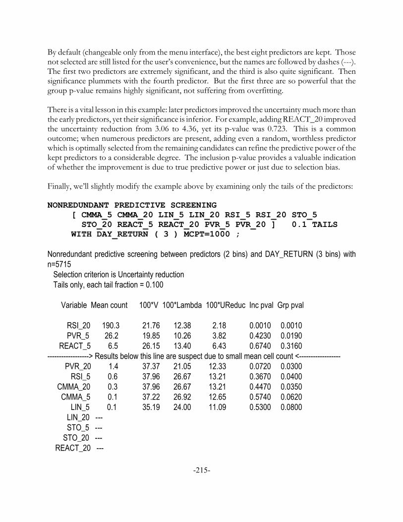
By default (changeable only from the menu interface), the best eight predictors are kept. Thosenot selected are still listed for the user’s convenience, but the names are followed by dashes (---). The first two predictors are extremely significant, and the third is also quite significant. Thensignificance plummets with the fourth predictor. But the first three are so powerful that thegroup p-value remains highly significant, not suffering from overfitting.

There is a vital lesson in this example: later predictors improved the uncertainty much more thanthe early predictors, yet their significance is inferior. For example, adding REACT_20 improvedthe uncertainty reduction from 3.06 to 4.36, yet its p-value was 0.723. This is a commonoutcome; when numerous predictors are present, adding even a random, worthless predictorwhich is optimally selected from the remaining candidates can refine the predictive power of thekept predictors to a considerable degree. The inclusion p-value provides a valuable indicationof whether the improvement is due to true predictive power or just due to selection bias.

Finally, we’ll slightly modify the example above by examining only the tails of the predictors:

NONREDUNDANT PREDICTIVE SCREENING[ CMMA_5 CMMA_20 LIN_5 LIN_20 RSI_5 RSI_20 STO_5 STO_20 REACT_5 REACT_20 PVR_5 PVR_20 ] 0.1 TAILSWITH DAY_RETURN ( 3 ) MCPT=1000 ;

Nonredundant predictive screening between predictors (2 bins) and DAY_RETURN (3 bins) withn=5715 Selection criterion is Uncertainty reduction Tails only, each tail fraction = 0.100

Variable Mean count 100*V 100*Lambda 100*UReduc Inc pval Grp pval

RSI_20 190.3 21.76 12.38 2.18 0.0010 0.0010 PVR_5 26.2 19.85 10.26 3.82 0.4230 0.0190 REACT_5 6.5 26.15 13.40 6.43 0.6740 0.3160------------------> Results below this line are suspect due to small mean cell count <------------------ PVR_20 1.4 37.37 21.05 12.33 0.0720 0.0300 RSI_5 0.6 37.96 26.67 13.21 0.3670 0.0400 CMMA_20 0.3 37.96 26.67 13.21 0.4470 0.0350 CMMA_5 0.1 37.22 26.92 12.65 0.5740 0.0620 LIN_5 0.1 35.19 24.00 11.09 0.5300 0.0800 LIN_20 --- STO_5 --- STO_20 --- REACT_20 ---

-215-

There are several items to note concerning these results:

! Performance measures in this example, which employed only the tails (most extremevalues) of the predictors showed predictability very much greater than in the priorexample, which used the entire distribution.

! Restricting data to tails caused the mean count per cell to drop much more rapidly thanwhen the entire distribution was used. As a result we can trust this report for only thefirst three predictors.

! The order of selection is different, indicating that the information in just the tails can bedifferent from the information in the entire distribution.

! Only one predictor had a significant inclusion p-value. Remember that this procedureis different from the chi-square procedure of the prior section. The chi-square proceduretested each indicator separately. On the other hand, the nonredundant predictorprocedure here tests them sequentially, evaluating the successive inclusion of morepredictors. So what we see here is that the information in the tails of RSI_20 containsall of the predictive power available in the set of candidates. No other candidate’s tailscan significantly add to the predictive information available in RSI_20's tails.

! The uncertainty reduction obtained using the tails of just RSI_20, which was 2.18percent, was almost three times as great as that obtained using the entire distribution ofall three significant predictors (0.86 percent) in the prior example! So although we paya high price in mean per-cell count by using tails only, the increase in predictive powerwith fewer predictors is nearly always a worthy tradeoff.

! Note that it is possible for these predictive power measures to decrease as we add apredictor. This is extremely rare for Uncertainty reduction and Lambda, essentially apathological situation. However, it is fairly common for Cramer’s V and is a natural partof its definition. Of course, once the cell count becomes small, all calculations becomeunreliable.

-216-

Triggering Trades With States and Events

By default, every case in the dataset is presented to models during training and testing. In somesituations, it can be useful to allow the possibility of trades for only a subset of the dataset. Wemay wish to allow trading only when the market is in a certain state, or when a certain eventoccurs. This is enabled with the following commands:

TRIGGER ALL VarName ;TRIGGER FIRST VarName ;REMOVE TRIGGER ;

VarName is the name of a variable that will define the trigger. The trigger variable should ideallybe binary 0/1, although this is not required. The threshold for triggering is 0.5. Values greaterthan this are treated as true and values less than or equal to this are considered to be false.

The TRIGGER ALL command allows trades whenever the trigger variable is true. The auditlog will note how many cases and the percent of the database have the value true.

The TRIGGER FIRST command allows trades for only the first day (or bar) in a string of truedays (bars) in the same market. In other words, a trade is allowed for days in which the triggervariable is true AND the trigger variable is false for the prior day in that market. The day priorto the first day in the database is assumed to be false. The audit log will note how many cases aretrue and how many are first true.

The trigger variable may be part of the database, or it may be an expression transform.

The REMOVE TRIGGER command removes the trigger and makes the entire database eligiblefor trading.

You may use multiple triggers in a script file to perform multiple tests. For example, thefollowing commands would test two different trigger scenarios, and then test the entire database:

TRIGGER ALL HiTrig ;CROSS VALIDATE BY YEAR ;TRIGGER ALL LoTrig ;CROSS VALIDATE BY YEAR ;REMOVE TRIGGER ;CROSS VALIDATE BY YEAR ;

Cross-sectional and pooled indicators are computed without regard to trigger states. If theFRACTILE THRESHOLD option is used, only triggered cases take part in the rank ordering. In this situation, it is recommended that the trigger variable be based on an index.

-217-

CUDA Processing

If your computer contains a CUDA-enabled device, it can be used for accelerating someapplications. (Currently, only GRNN training can use a CUDA device.) In order to implementCUDA acceleration, the following line must appear anywhere in a script control file:

CUDA ;

CUDA processing will occur after this command is encountered. Thus, you should insert thiscommand before any TRAIN, CROSS VALIDATE, or WALK FORWARD command if youwant it to employ CUDA acceleration.

-218-

Performance statisticsThis section discusses the performance statistics that appear in the audit and report logs. Different applications will use different statistics, so it is likely that not all of the informationpresented here will appear in every application. Here is a section of the output from awalkforward run, with a running commentary:

Firs t, th e y e ar an d n u m b e r o f train in g an d te s tin g c as e s is lis te d .

-----------------------------------------------------YEAR 2006 training 35497 cases, testing 4399-----------------------------------------------------

Th e m o d e l ab o u t to b e p re s e n te d , as w e ll as its targ e t an d o p tim izatio n c rite rio n (p f ;p ro f it fac to r) , is n am e d an d d e s c rib e d . Th e fac t th at th e u s e r s p e c if ie d th e FRACTILETHRESHOLD an d XVAL STEPWISE o p tio n s is n o te d . Th e u s e r d e m an d s th at at le as t0.1 o f th e train in g c as e s lie o u ts id e e ac h th re s h o ld (u p p e r an d lo w e r) . Th e b e s t m o d e lh as a c rite rio n o f -0.2592, w h ic h is th e lo g o f its p ro f it fac to r. Th is is n o t a g o o d o m e n ,as it s h o w s th at e v e n th e b e s t in -s am p le m o d e l lo s e s m o n e y in a c ro s s -v alid ate de v alu atio n . Th e m o d e l is lin e ar re g re s s io n (LINREG) w ith o n e p re d ic to r c h o s e n . Th atp re d ic to r’s c o e f f ic ie n t an d th e c o n s tan t o f f s e t are p rin te d fo r th e u s e r’s e d if ic atio n .

LINREG Model VAL1 predicting RETURN1FRACTILE THRESHOLD specifiedXVAL Optimizing pf with min fraction=0.100 (Final best crit= -0.2592)Regression coefficients: 0.019780 FILTER_VALUE 2.362443 CONSTANT

-219-

In -s am p le p e rfo rm an c e re s u lts n o w ap p e ar. Th e u p p e r th re s h o ld (o u te r, o r p rim ary ) is0.79832, w h ic h re s u lts in 3550 o f th e 35497 train in g c as e s e q u alin g o r e xc e e d in g it. Th isis te n p e rc e n t o f th e train in g c as e s , w h ic h is to b e e xp e c te d b e c au s e th e u s e r s p e c if ie dFRACTILE THRESHOLD and th e o p tim ize d u p p e r th re s h o ld is ab o u t 0.8. Th e lo w e rth re s h o ld an d in n e r th re s h o ld s are s im ilarly d is p lay e d . O th e r p e rfo rm an c e c rite riain c lu d e th e m e an s q u are d e rro r, R-s q u are d (w h ic h c an b e n e g ativ e if th e m o d e l is an ti-p re d ic tiv e ) , an d are a u n d e r th e ROC c u rv e . Th e b u y -an d -h o ld an d s e ll-s h o rt-an d -h o ldp ro f it fac to rs (re c ip ro c als , o f c o u rs e ) are p rin te d fo r re f e re n c e . If w e w e re to b u y allc as e s ab o v e th e u p p e r th re s h o ld an d s e ll all c as e s b e lo w th e lo w e r th re s h o ld , w e w o u ldac h ie v e a p ro f it fac to r o f 0.887. Th is lo s in g s trate g y is e xp e c te d w h e n w e n o te th at th istrain in g p e rio d is s tro n g ly u p -tre n d in g (b u y -an d -h o ld p f=2.4) b u t th e s e p arate lyo p tim ize d th re s h o ld s re s u lt in m o re th an tw ic e as m an y s h o rt trad e s as lo n g trad e s . Wh e n th e lo n g an d s h o rt s id e s are s e p arate d , w e s e e th at a lo n g -o n ly s trate g y re s u lts ina p ro f it fac to r o f 2.966, w h ic h is 1.236 tim e s th e b u y -an d -h o ld p ro f it fac to r o f 2.4. Th es h o rt s id e is s im ilarly s h o w n . Fin ally , s in c e th e u s e r s p e c if ie d th e FRACTILETHRESHOLD o p tio n , p ro f it fac to rs f ro m b alan c e d p o s itio n s w ith 0.01, 0.1, 0.25, an d 0.5trad e s o u ts id e th e th re s h o ld are s h o w n . Ob s e rv e th at th e s e are all p ro f itab le , in s h arpc o n tras t to th e u n b alan c e d lo n g /s h o rt s trate g y .

Outer hi threshold = 0.79832 with 3550 of 35497 cases at orabove (10.00 %)Inner hi threshold = 0.65001 with 4551 of 35497 cases at orabove (12.80 %)Inner lo threshold = -0.41133 with 9935 of 35497 cases ator above (27.99 %) Outer lo threshold = -0.51498 with 8591 of 35497 cases ator below (24.20 %)MSE = 71.04773 R-squared = 0.00032 ROC area = 0.53523Buy-and-hold profit factor = 2.400 Sell-and-hold = 0.417Dual-thresholded outer PF = 0.887Dual-thresholded inner PF = 0.803 Outer long-only PF = 2.966 Ratio = 1.236 Inner long-only PF = 2.505 Ratio = 1.044 Inner short-only PF = 0.441 Ratio = 1.058 Outer short-only PF = 0.493 Ratio = 1.183Balanced (0.01 each side) PF = 1.352Balanced (0.05 each side) PF = 1.295Balanced (0.10 each side) PF = 1.251Balanced (0.25 each side) PF = 1.220Balanced (0.50 each side) PF = 1.133

-220-

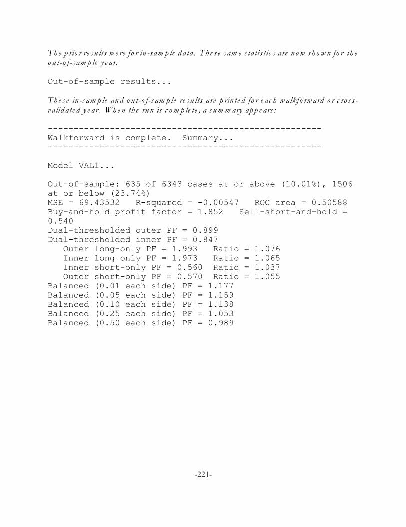
Th e p rio r re s u lts w e re fo r in -s am p le d ata. Th e s e s am e s tatis tic s are n o w s h o w n fo r th eo u t-o f -s am p le y e ar.

Out-of-sample results...

Th e s e in -s am p le an d o u t-o f -s am p le re s u lts are p rin te d fo r e ac h w alkfo rw ard o r c ro s s -v alid ate d y e ar. Wh e n th e ru n is c o m p le te , a s u m m ary ap p e ars :

-----------------------------------------------------Walkforward is complete. Summary...-----------------------------------------------------

Model VAL1...

Out-of-sample: 635 of 6343 cases at or above (10.01%), 1506at or below (23.74%)MSE = 69.43532 R-squared = -0.00547 ROC area = 0.50588Buy-and-hold profit factor = 1.852 Sell-short-and-hold =0.540Dual-thresholded outer PF = 0.899Dual-thresholded inner PF = 0.847 Outer long-only PF = 1.993 Ratio = 1.076 Inner long-only PF = 1.973 Ratio = 1.065 Inner short-only PF = 0.560 Ratio = 1.037 Outer short-only PF = 0.570 Ratio = 1.055Balanced (0.01 each side) PF = 1.177Balanced (0.05 each side) PF = 1.159Balanced (0.10 each side) PF = 1.138Balanced (0.25 each side) PF = 1.053Balanced (0.50 each side) PF = 0.989

-221-

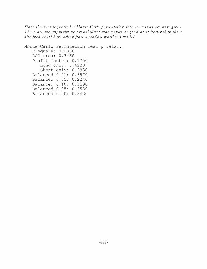
Sin c e th e u s e r re q u e s te d a Mo n te -Carlo p e rm u tatio n te s t, its re s u lts are n o w g iv e n . Th e s e are th e ap p ro xim ate p ro b ab ilitie s th at re s u lts as g o o d as o r b e tte r th an th o s eo b tain e d c o u ld h av e aris e n f ro m a ran d o m w o rth le s s m o d e l.

Monte-Carlo Permutation Test p-vals... R-square: 0.2830 ROC area: 0.3460 Profit factor: 0.1750 Long only: 0.4220 Short only: 0.2930 Balanced 0.01: 0.3570 Balanced 0.05: 0.2240 Balanced 0.10: 0.1190 Balanced 0.25: 0.2580 Balanced 0.50: 0.8430

-222-

Sin c e th is ru n w as te s tin g a f ilte r m o d e l (Hau g e n Alp h a in th is c as e ) , a tab le ap p e arsc o m p arin g th e p e rfo rm an c e o f th e o rig in al f ig u re s b e in g f ilte re d v e rs u s th e m o d e l ju s tte s te d . Th e le f tm o s t c o lu m n s h o w s th e f rac tio n o f th e c as e s b e in g ke p t. Th e n e xtc o lu m n s h o w s th e p ro f it fac to r o b tain e d b y b u y in g th e s p e c if ie d h ig h e s t f rac tio n o f th ed ata b e in g f ilte re d . Th e n e xt c o lu m n s h o w s th e c o rre s p o n d in g p ro f it fac to r o b tain e d b yb u y in g th at f rac tio n o f th e m o d e l’s h ig h e s t p re d ic tio n s . Th e las t tw o c o lu m n s s h o w th ec o rre s p o n d in g p ro f it fac to rs o n th e s h o rt s id e . In th is c as e , th e o rig in al f ilte r d ata an dth e m o d e l h av e id e n tic al p e rfo rm an c e b e c au s e th e o n ly v ariab le s e le c te d fo r e ac h trialy e ar w as alp h a its e lf , an d th e c o e f f ic ie n t w as alw ay s p o s itiv e ! So th e s e m o d e ls aretran s p are n t, g iv in g e xac tly th e s am e ran ke d p re d ic tio n s as th e o rig in al f ilte r d ata. Wes e e , fo r e xam p le , th at if w e w e re to b u y th e larg e s t 25 p e rc e n t o f th e alp h as o r m o d e lp re d ic tio n s , w e w o u ld o b tain a p ro f it fac to r o f 1.904. Sim ilarly , if w e s e ll th e sm alle s t o n ep e rc e n t o f th e alp h as o r m o d e l p re d ic tio n s , w e w o u ld o b tain a p ro f it fac to r o f 0.911. Wh e n w e train a p rac tic al m o d e l, w e h o p e th at m o s t o r all o f th e m o d e l p ro f it fac to rse xc e e d th e f ilte r-v ariab le p ro f it fac to rs .

Filter versus model profit factors (raw data) for variousextremesFraction Filter long Model long Filter short Model short 0.01 1.579 1.579 0.911 0.911 0.05 1.860 1.860 0.700 0.700 0.10 1.984 1.984 0.635 0.635 0.25 1.904 1.904 0.572 0.572 0.50 1.822 1.822 0.531 0.531 0.75 1.886 1.886 0.545 0.545 0.90 1.888 1.888 0.544 0.544 0.95 1.877 1.877 0.540 0.540 0.99 1.860 1.860 0.539 0.539

-223-

Permutation TrainingAn essential part of model-based trading system development is training a model (or set ofmodels, committees, et cetera) to predict the near-future behavior of the market. Traininginvolves finding a set of model parameters that maximizes a measure of performance within ahistorical dataset. Much of the time, the resulting performance will be excellent. However, thissuperb performance is at least partially due to the fact that the training process treated noise orother unique properties of the data as if they were legitimate patterns. Because such patterns areunlikely to repeat in the future, the performance obtained due to training is optimistic, oftenwildly so.

This undue optimism requires the responsible developer to answer two separate and equallyimportant questions:

1) What is the probability that if the trading system (model(s) et cetera) were truly worthless,good luck could have produced results as good as those observed? We want thisprobability, called the p-value, to be small. If it turns out that there is an uncomfortablylarge probability that a truly worthless system could have given results as good as whatwe obtained just by being lucky, we should be skeptical of the trading system at hand.

2) What is the average performance that can be expected in the future (assuming that themarket behavior does not change, which of course may be an unrealistic but unavoidableassumption)?

It is vital to understand that these are different, largely unrelated questions, and a responsibledeveloper will require a satisfactory answer to both of them before signing off on real-life trading. It is possible, especially if extensive market history has been tested, for the answer to the firstquestion to be a nicely small probability, even though the expected future performance ismediocre, hardly worth trading real money. It is also possible for the expected futureperformance to be enticing, but with a high probability of having been obtained by random goodluck from a truly worthless system. Thus, we need both properties: it must be highly unlikelythat a worthless system would have had sufficient good luck to do as well as we observed, andthe expected future performance must be good enough to be worth putting down real money.

The standard method for answering the second question, and sometimes the first as well, iswalkforward testing. The performance obtained in the pooled out-of-sample (OOS) period isan unbiased estimate of future performance. (Note that the term unbiased is used here in theloose sense of being without prejudice, as opposed to the much stronger statistical sense.) If theOOS cases are independent (which they would not be if the targets look ahead more than onebar), an ordinary bootstrap test can answer the first question. Even if the cases have serialdependence, special bootstraps can do a fairly good job of answering the first question.

-224-

But the problem with the walkforward approach is that it discards a lot of data, often themajority of historical data. Only the pooled OOS data can be used to answer the two questions. This is a high price to pay. There is an alternative approach to answering the first question, andwhich can also provide at least a decent hint of an answer to the second question, while usingall available historical data.

Unfortunately, this alternative approach has a high price of its own: time. Training time ismultiplied by a factor of at least 100, and as much as 1000 if a thorough job is to be done. Thisprecludes some analyses. But it is a great addition to the developers toolbox.

This approach is invoked with the following command:

TRAIN PERMUTED Nreps ;

If this command appears, no database can be read or appended. This is because all indicators andtargets must be able to be recomputed from the original and permuted market(s). Thisrecomputation would obviously not be possible for precomputed indicators and targets in adatabase. Also, the REMOVE ZERO VOLUME command described on Page 3 must appearbefore the READ MARKET HISTORIES command.

TRAIN PERMUTED operates similarly to the ordinary TRAIN command, except that inaddition to the usual computation of indicators and targets from the data, it also recomputesindicators and targets, and retrains all models, Nreps-1 times. Each of these repetitions is doneon market histories whose changes have been shuffled. Thus, the permuted markets haveexactly the same bar-to-bar changes as the original, unpermuted markets, but in a different order. This random shuffling obviously destroys any predictable patterns in the markets, giving us alarge number of examples of truly worthless trading systems; no matter how ‘good’ a tradingsystem may be, it will be worthless when presented with random market data! Some of theseshuffled market histories will allow the trained trading systems to be lucky, and others will not. Thus, by counting how often we obtain a trading system from shuffled data whose performanceis at least as good as that obtained from the original, unshuffled history, we can directly answerthe first question.

Another way of looking at this algorithm is by realizing that if the trading system beingdeveloped is truly worthless, presenting it with real market data is no better than presenting itwith random data. Its performance is no more likely to be outstanding than permutedperformance. We would expect its performance to be somewhere in the middle of the heap,better than some and worse than others. On the other hand, suppose our trading system is trulyable to detect authentic patterns in market data. Then we would expect its performance on thereal data to exceed that of most or all of the systems developed on shuffled data.

-225-

Figure 14: Histogram of TRAIN PERMUTED performance

In particular, suppose our trading system is truly worthless, and also suppose that we have Nrepstrading results. One of these is from the original, unpermuted data, and the others are fromshuffled data. Then there is a 1/Nreps probability that the original will be the best (none of theothers exceeded it). There is a 2/Nreps probability that it will be at least second-best (at mostone other exceeded it) and so forth. This can be visualized by imagining the performancemeasures laid out in a sorted line and knowing that if the system is worthless, it can land in anyposition with equal probability. In general, if k shuffled performance measures equal or exceedthe unshuffled measure, the probability addressed by Question 1 above is (k+1)/Nreps.

This method of estimating probabilities of performance results can be seen in Figure 14 below. This is a histogram of the long-only profit factors obtained by a model called LIN_LONG whentrained on 99 randomly shuffled market histories as well as the original unshuffled history. Theprofit factor from the original data is shown as a vertical red line. Note that this performanceis one of the best, with a probability of 0.06 under the null hypothesis that the model isworthless.

-226-

(10)

The Components of Performance

The primary task of permutation training is estimating the probability that a worthless systemcould benefit from good luck sufficiently to attain the observed performance level. Thisprovides an answer to Question 1 shown at the start of this chapter. However, Question 2 isequally important: What level of performance can we expect in the future? The gold standardfor answering this question is walkforward testing. However, as a byproduct of probabilityestimation we can compute a rough but still useful estimate of one specific measure of futureperformance: Total return.

The fundamental basis of this estimation is the relationship among four loosely defined aspectsof performance:

To tal - The total return of the trading system after training

Skill - The true ability of the trading system to find and profit from authentic market patterns

Tre n d - If the market significantly trends up (or down) and the trading system is unbalanced infavor of long(or short) positions, this unbalance will generate profits on average evenwithout intelligent individual trade decisions. If the market trend is large, and if thetrading system development software has the ability to create unbalanced systems (themost common situation), the software will favor unbalanced systems that take advantageof the trend, even if these systems do not make many intelligent individual trades.

Bias - The process of training the system induces training bias by tuning its trade decisions to notonly the authentic patterns represented in the dataset, but also to patterns that are uniqueto the historical dataset and may not be repeated in later use. If the system developmentsoftware employs very powerful models, these models may go to great lengths to captureevery pattern they see in the data, authentic and temporary, with the result that apparentperformance will be greatly inflated.

Although Equation 10 below is far from a rigorous statement of how these four items arerelated, it is usually fairly close when these quantities are components of the total return of thetrading system, and it is a useful mental tool for understanding the performance of a tradingsystem after it has been trained:

The market data is permuted in such a way that any underlying trend is almost exactly preserved. As a result, the training algorithm will have the opportunity to generate unbalanced systems thattake advantage of the trend, just as they do with the unpermuted market history. Therefore, we

-227-

(11)

(12)

can expect that the Trend component of the total return will be about the same for the permutedmarkets as for the unpermuted market.

Also, the permuted markets will, on average, present to the training algorithm the sameopportunity to capitalize on inauthentic patterns as did the unpermuted market. Thus, we canexpect that the Bias component of the permuted returns will, on average, be about the same asthat for the unpermuted return.

The only difference between the returns from the unpermuted and the permuted markets is theSkill component, which cannot exist in permuted data. In other words, Equation 11 belowrepresents the average total return obtained from training on permuted markets.

As a point of interest, look back at Figure 14 on Page 226. That figure is based on profit factors,while the equations just shown are more applicable to total return. Nonetheless, the principleis the same for either measure of performance. The bars in this histogram represent the valuesof Equation 11 above (plus the single observation for the unpermuted market, which is also usedto compute the histogram). The red vertical bar is the value represented by Equation 10 above. We can thereby see the effect of Skill on performance relative to the performance of the trainedtrading systems when Skill is not involved. If the Skill component is significant, we wouldexpect the vertical red bar to be on the far right side of the histogram, pushed there by the abilityof the trading system to find authentic patterns in the market. Conversely, if the Skillcomponent of performance is small, the red bar is more likely to be somewhere in the interiormass of the histogram.

Additional information can be gleaned from the permutation training by analyzing Equation 11in more detail. When the trading system is trained by maximizing performance on a permuteddataset, the training algorithm will attempt to simultaneously maximize both components ofEquation 11: it will try to produce an unequal number of long and short trades (assuming thatthe user allows unbalanced systems) in order to take advantage of any long-term trend in themarket(s), and it will try to take individual trades in such a way as to capitalize on any patternsit finds in the data. Of course, since it is operating on randomly permuted data, any patterns itfinds are inauthentic, which is why the Skill component plays no role.

Now suppose we have a system that makes only long trades, and it does so randomly; individualtrades are made with no intelligence whatsoever. Equation 12 shows its expected return:

-228-

(13)

(14)

In this equation, BarsLong is the number of bars in which a long position is signaled, andTotalNumberOfBars is the number of bars in the entire dataset whose performance is beingevaluated. This ratio is the fraction of the number of bars in which a long position is signaled. Looked at another way, this ratio is the probability that any given bar will signal a long position. TotalTargets is the sum of the target variable across all bars. This will be positive for markets witha long-term upward trend, negative for those with downward trend, and zero for a net flatmarket. So if our system is without intelligence, with signals randomly given, we will on averageobtain this fraction (the fraction of time a long signal is given) of the total return possible.

A similar argument can be made for a short-only system, although the sign would be flippedbecause for short systems a positive target implies a loss, and a negative target implies a win. Combining these two situations into a single quantity gives Equation 13, the expected net return(the Trend performance component) from a random system that contains both long and shortsignals.

When we train a trading system using a permuted market, we can note how many long and shorttrades it signaled and then use Equation 13 to determine how much of its total return is due toposition imbalance interacting with long-term trend. Anything above and beyond this quantityis training bias due to the system learning patterns that happen to exist in the randomly shuffledmarket. This training bias can be estimated with Equation 14.

It would be risky to base a Bias estimate on a single training session. However, as long as we arerepeating the permutation and training many times to compute the probability of the observedreturn happening by just good luck, we might as well average Equation 14 across all of thosereplications. If at least 100 or so replications are used, we should get a fairly decent estimate ofthe degree to which the training process is able to exploit inauthentic patterns and therebyproduce inflated performance results.

Two thoughts are worth consideration at this point:

! TSSB allows various BALANCED criteria which force an equal number of long andshort positions in multiple markets. In this case, Trend will be zero.

! Powerful models will generally produce a large Bias, while weak models (not necessarilya bad thing) will produce small Bias.

-229-

(15)

(16)

Now that the Bias can be estimated, we can go one or two steps further. Equation 10 can berearranged as shown in Equation 15 below.

This equation shows that if we subtract the Bias estimated with Equation 14 from the totalreturn of the system that was trained on the original, unpermuted data, we are left with the Skillplus Trend components of the total return. Many developers will wish to stop here. Theirthought is that if a market has a long-term trend, any effective trading system should takeadvantage of this trend by favoring long or short positions accordingly. However, anotherschool of thought says that since deliberately unbalancing positions to take advantage of trenddoes not involve actual trade-by-trade intelligent picking, the trend component should beremoved from the total return. This can be effected by applying Equation 13 to the originaltrading system and subtracting the Trend from the UnbiasedReturn, as shown in Equation 16below.

This difference, the Skill component of Equation 10, is often called the Benchmarked returnbecause the NetExpectedReturn (Trend component) defined by Equation 13 can be thought of asa benchmark against which to judge actual trading performance.

These figures are all reported in the audit log file, with p-values for the profit factor and totalreturn printed first. Here is a sample:

Net profit factor p = 0.0600 return p = 0.0400Training bias = 52.3346 (67.1255 permuted return minus 14.7909 permuted benchmark)Unbiased return = 55.4320 (107.7665 original return minus 52.3346 training bias = skill + trend)Benchmarked return = 39.8372 (55.4320 unbiased return minus 15.5947 original benchmark = skill)

The Training bias line is Equation 14, with the term benchmark referring to Trend in the equation,and these figures averaged over all replications. This figure (52.3346 here) is the approximatedegree to which the training process unjustly elevates the system’s total return due to learningof inauthentic patterns.

The Unbiased return line is Equation 15, the actual return that we could expect in the future afteraccounting for the training bias. This figure includes both the true skill of the trading system aswell as the component due to unbalanced trades that take advantage of market trend.

The Benchmarked return line is Equation 16. This is the pure Skill component of the total return.

-230-

Permutation Training and Selection Bias

Up to this point we have discussed only training bias, which is usually dominated by modelslearning patterns of noise as if they were authentic patterns. There are other sources of trainingbias, such as incomplete representation of all possible patterns in the available history. However,these other sources are generally small and unavoidable. So what we have covered is sufficientto handle training bias in most practical applications.

However, there is another potential source of bias that inflates performance in the dataset abovewhat can be expected in the future. This is selection bias, and it occurs when we choose one ormore trained models from among a group of competitors. Bias occurs in the selection processbecause some of the models will have been lucky while others will have been unlucky. Thosemodels that were lucky will be more likely to be selected than those that were unlucky, yet theirluck, by definition, will not hold up in the future. Thus, the performance of the best modelsfrom among a set of competitors will likely deteriorate in the future as the luck that propelledthem to the top vanishes.

If the user has employed any Portfolios of type IS (in-sample) in the script file, the TRAINPERMUTED command will properly handle them, and the p-values and total returnperformance measures (unbiased and benchmarked) will be correct, or at least as correct as ispossible under the loose assumptions of the technique. In other words, the selection biasinherent in the choice of an optimal subset will be accounted for in both the p-values and in theunbiased and benchmarked total returns.

There is one vital aspect of this to consider, though. Recall from the earlier discussion of theIS type of Portfolio that this is a potentially dangerous type. This is because if one or more ofthe competing models is extremely powerful, its in-sample performance will be unjustifiablyexcellent. As a result, it will likely be included in a Portfolio. This will, in turn, make this aseriously overfitted Portfolio. Of course, this will be detected in the permutation test, but thatis little comfort if you are faced with a poorly performing Portfolio..

The proper way to handle this problem is to use the OOS type of Portfolio. Unfortunately, theTRAIN PERMUTED operation cannot handle OOS Portfolios. These can be evaluated onlyin a WALK FORWARD test because they need OOS model results for selecting the Portfoliocomponents. A future release of TSSB may include a permutation version of this test.

-231-

An example of poor IS portfolio creation due to an overfit model can be seen in the exampleshown below. In this example, five weak models are defined: LIN1 through LIN5. They areall identical, using the EXCLUSION GROUP option to guarantee that their solo predictors aredifferent. As stated earlier, this option is excellent for generating committee members, butprobably not the best way to generate Portfolio candidates. Only LIN1 is shown here.

A strong model, LIN_POWER, is also defined. Unlike LIN1 through LIN5, which allow onlyone predictor, this one allows four predictors, which is almost certainly excessive. Finally, aPortfolio is defined which optimally selects two of these six candidate Models. It is LONGONLY, so the six models all select their predictors by maximizing the long profit factor.

MODEL LIN1 IS LINREG [ INPUT = [ CMMA_5 CMMA_20 LIN_5 LIN_20 RSI_5 RSI_20

STO_5 STO_20 REACT_5 REACT_20 PVR_5 PVR_20 ] OUTPUT = DAY_RETURN MAX STEPWISE = 1 CRITERION = LONG PROFIT FACTOR MIN CRITERION FRACTION = 0.1 EXCLUSION GROUP = 1 ] ;

MODEL LIN_POWER IS LINREG [ INPUT = [ CMMA_5 CMMA_20 LIN_5 LIN_20 RSI_5 RSI_20

STO_5 STO_20 REACT_5 REACT_20 PVR_5 PVR_20 ] OUTPUT = DAY_RETURN MAX STEPWISE = 4 CRITERION = LONG PROFIT FACTOR MIN CRITERION FRACTION = 0.1 ] ;

PORTFOLIO Port_Power [ MODELS = [ LIN1 LIN2 LIN3 LIN4 LIN5 LIN_POWER ] TYPE = OPTIMIZE 2 IS NREPS = 1000 LONG ONLY EQUALIZE PORTFOLIO STATS ] ;

The Portfolio optimizer selected LIN4 and LIN_POWER (of course) as the best components. Permutation training produced the distribution of profit factors shown on the next page.

-232-

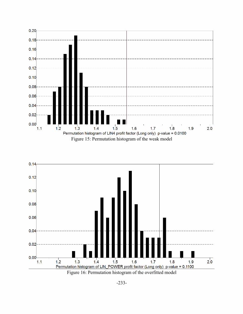
Figure 15: Permutation histogram of the weak model

Figure 16: Permutation histogram of the overfitted model

-233-

Look at the histograms shown on the prior page. Observe that, as expected, LIN_POWER hada much higher profit factor than LIN4. This is because this is an in-sample computation, andLIN_POWER is a much more powerful model than LIN4. But along with this greater profitfactor for the original data, the profit factors of shuffled data were also greater forLIN_POWER than for LIN4; LIN_POWER’s histogram is considerably shifted to the right ofthat of LIN4. In fact, LIN_POWER’s p-value of 0.11 is very inferior to that of LIN4, 0.01.

Finally, let’s explore the performance partitioning for these models and the optimal Portfolio. These are shown on the next page. Note first that the p-values for the return have the oppositeordering as those for the profit factor (0.1 versus 0.01). This is not unusual; total return andprofit factor have surprisingly little relationship. It may be that one model has few but excellenttrades, resulting in a high profit factor and low total return, while another model has many tradesthat are only moderately good. This model may have a profit factor barely exceeding one, yethave a high total return by virtue of its large number of trades. Experience shows that profitfactor is a vastly superior measure of performance than total return.

The most salient figure is the training bias: the weak model LIN4 has a training bias of 37.4672,while the strong model LIN_POWER has a training bias of 58.8356. This great disparity shouldnot be surprising. Interestingly enough, when the bias is subtracted from the performance ofeach model, the unbiased returns of 59.6410 for LIN4 and 57.8350 for LIN_POWER arealmost equal. The benchmarked returns are also almost equal. So we see that, at least in termsof total return, the weak and the strong model have about the same skill at detecting validpatterns in the market data. It’s just that the more powerful model’s returns are inflated by itsgreater ability to learn inauthentic patterns in the data.

Finally, let’s look at the Portfolio results. Because its definition includes the EQUALIZEPORTFOLIO STATS option, all of these figures are based on the average of its two components,not their sum. We see that the Portfolio’s training bias is nearly as great as that of LIN_POWER,probably reflecting the fact that this bias figure includes selection bias as well as the training biasof the two component models. Without the selection bias (if this were a fixed Portfolio), thetraining bias would have equaled the mean of the training biases of the two component models,or (37.4672 + 58.8356) / 2 = 48.1514. However, this model training bias is inflated further bythe selection bias inherent in creating the optimal portfolio. This raises the Portfolio’s trainingbias considerably.

After subtracting the training bias from the raw total return of the Portfolio, we see that theunbiased return is a little less than that of the two component models. This is probably justrandom variation. The important point is that the Portfolio results are in line with thecomponents because the algorithm has compensated not only for the models’ training bias, butthe Portfolio’s selection bias as well.

-234-

MODEL LIN4 Long profit factor p = 0.0100 return p = 0.1000 Training bias = 37.4672 (57.6183 permuted return minus 20.1511 permuted benchmark) Unbiased return = 59.6410 (97.1082 original return minus 37.4672 training bias = skill + trend) Benchmarked return = 43.3659 (59.6410 unbiased return minus 16.2751 original benchmark = skill)

MODEL LIN_POWER Long profit factor p = 0.1100 return p = 0.0100 Training bias = 58.8356 (73.1141 permuted return minus 14.2786 permuted benchmark) Unbiased return = 57.8350 (116.6705 original return minus 58.8356 training bias = skill + trend) Benchmarked return = 42.2402 (57.8350 unbiased return minus 15.5947 original benchmark = skill)

PORTFOLIO PORT_POWER profit factor p = 0.0400 return p = 0.0500 Training bias = 53.7958 (72.4237 permuted return minus 18.6279 permuted benchmark) Unbiased return = 53.0935 (106.8894 original return minus 53.7958 training bias = skill + trend) Benchmarked return = 37.1586 (53.0935 unbiased return minus 15.9349 original benchmark = skill)

-235-

Multiple-Market Considerations

When the TRAIN PERMUTED command is executed in a multiple-market situation, operationbecomes slightly more complicated. The issue is that inter-market correlation must br preserved. A fundamental assumption of permutation tests is that all permutations must be equally likelyto have occurred in real life. For example, it is well known that in times of large moves, marketstend to move together. When some world crisis arises, most markets go down. When goodeconomic news is broadcast, most markets rise. If the markets were permuted separately, thiscoherence would be lost and the permutation test would be invalidated.

This implies that every market must have data available for every date. Otherwise it would beimpossible to swap dates with data in some markets and not in others. In order to accomplishthis, the first step in permutation training is to pass through the market history and eliminate alldates whose market set is incomplete. This results in a message similar to the following beingprinted in the audit log file:

NOTE... Pruning multiple markets for simultaneous permutation reduced the number of market-dates from 503809 to 414427.The model(s) about to be printed and all permutation results reflect this reduced dataset and will differ from prior and subsequent results.

This message informs the user as to how many market-dates had to be removed from the historyfiles. It also reminds the user that the results about to be shown reflect the market histories afterthis reduction, and hence they will generally be different from results of an ordinary TRAINoperation performed before or after the TRAIN PERMUTED operation.

If any dates had to be eliminated, then after the TRAIN PERMUTED operation is completeand all of its results are printed, the dates will be restored and as a convenience for the user thetrading system will be trained with the complete dataset. A message similar to the following willbe printed to make it clear to the user what is happening:

NOTE... Permutation is complete. Prior to permutation wehad to reduce the number of market-dates so thatevery date had all markets.The original markets have now been restored.All models will now be re-trained with the originalmarket data. The results you are about to see reflectthis original data, before pruning.

-236-

Walk Forward PermutationIn order to be reasonably confident that a trading system will perform satisfactorily when it isput into operation, one needs to evaluate four performance statistics. These are:

In -s am p le p e rfo rm an c e - This is the profit obtained from the backtest used in thedevelopment of the system. Because this profit most likely has been obtained throughoptimization of one or more training parameters, it will have an upward bias calledtraining bias. Thus, good in-sample profit is a necessary but not sufficient condition for a successful trading system. We can obtain this figure from TSSB using the TRAINcommand.

In -s am p le p -v alu e - This is the probability that the in-sample performance obtained from thebacktest, described in the prior paragraph, could have been obtained from a trulyworthless system that happened to get lucky by randomly capturing an unusual numberof profitable trades. Unless this p-value is small, we should not put much store in the in-sample performance, even if it is impressive. Remember that good in-sampleperformance is a necessary condition for having a good trading system. If there is anuncomfortably large probability that the performance obtained could have been due to nothing more than dumb luck, it may be that the true in-sample performance, that whichwould be obtained without the benefit of luck, would be so poor as to violate thenecessity requirement. This figure is obtained from TSSB with the TRAINPERMUTED command.

Ou t-o f -s am p le (OOS) p e rfo rm an c e - This is the profit obtained when the system is tested ondata which it has not seen during the development process. It is generally considered tobe unbiased, an honest indication of the performance that could be obtained on averagewhen the system is put into use. This figure is provided by TSSB with the WALKFORWARD command.

Ou t-o f -s am p le p -v alu e - This is the probability that the OOS performance described in theprior paragraph could have been obtained from a truly worthless system just by randomgood luck. This statistic is not generally available from commercial trading-system-development programs, and hence it is ignored by the vast majority of developers. Yetit is every bit as important to successful development as the three other statistics justdescribed. If a developer obtains a trading system that has good walkforwardperformance, that developer will be strongly inclined to conclude that he or she has apotential gold mine in hand and jump right into actual trading. This is justified by thecorrect thought that the OOS performance is unbiased. True enough. But luck stillplays a role, and if the OOS p-value is not small, an intelligent developer will be skeptical,

-237-

regardless of how good the OOS performance is. This statistic is obtained from TSSBusing the WALK FORWARD PERMUTED command, the topic of this section.

This command has exactly the same syntax as the ordinary WALK FORWARD command,except that the word PERMUTED is appended, and this is followed by the number ofpermutations desired, including the original unpermuted test. In most cases this number shouldbe at least 100, and 1000 is not unreasonable. Unfortunately, execution can be very slow, sotime constraints may limit the number of permutations specified.

For example, the following command would perform a permuted walkforward test beginningin the year 2000, using 5-year training periods, and perform this test 100 times (1 unpermutedand 99 permuted) to obtain the required p-value.

WALK FORWARD BY YEAR 5 2000 PERMUTED 100 ;

The p-values will be reported for the net return of every model, committee, oracle, and portfolioin the script file. There are no restrictions on the quantity or nature of models et cetera tested. The only restriction is that permuted walkforward cannot be performed in a script file in whicha database has been read, just as with the TRAIN PERMUTED command. As in that case, theprogram would need to be able to permute the market information that produced the indicatorsand targets in the database, and this of course is impossible! A future release of TSSB may allowpermuted training and walkforward when a database has been read, but this would be adangerous undertaking for the trading-system developer, as subtle interactions betweenpermuted and unpermuted data could easily subvert results.

It should be noted that performance statistics are computed slightly differently for portfoliosversus models, committees, and oracles. The algorithms are algebraically identical, but becausefloating-point calculations done on a computer are not exact, performance figures may differ bytiny amounts. The implication is that if one were to define a FIXED portfolio of a single model(pointless but legal), although one would expect that p-values would be identical for the modeland the portfolio, in practice the p-values can occasionally differ slightly. This is normal.

-238-

Trade Simulation and PortfoliosYou may follow a TRAIN, WALK FORWARD, or CROSS VALIDATE command with thePRESERVE PREDICTIONS command, and follow this with a TRADE SIMULATORcommand. This provides more extensive performance statistics than are provided by default,and it also allows you to execute slightly more sophisticated rules than those inherent in defaultoperation. The syntax of this command is as follows:

TRADE SIMULATOR Model Detail TradeRule PerformanceMeasure

Model names a model that is in the script file. Trades for this model will be simulated.

The Detail may be GLOBAL or BY MARKET. This option, although always required, isrelevant only if multiple markets are present. If you choose GLOBAL, only a summary withall markets pooled will be printed. If you choose BY MARKET, not only will the globalsummary be printed, but results for each individual market will also be printed. Note that thiswill produce a voluminous printout if a large number of markets are present. This option mustbe GLOBAL if an equity curve will be written or displayed.

The TradeRule must be one of the following: LONG ( Enter Maintain )LONG ( TRAINED Maintain )SHORT ( Enter Maintain )SHORT ( TRAINED Maintain )DUAL ( LongEnter LongMaintain ShortEnter ShortMaintain )DUAL ( TRAINED LongMaintain TRAINED ShortMaintain )

The rules that begin with LONG will take only long positions. The position will be openedwhen the model’s prediction equals or exceeds the Enter value, and it will be closed when theprediction drops below the Maintain value. Obviously, the Maintain value must not exceed theEnter value. Negative values are permitted.

If instead of specifying a numeric Enter value, you specify the keyword TRAINED, the positionwill be opened when the predicted value equals or exceeds the optimal in-sample valuedetermined during training. This is legal for cross validation and walkforward as well as ordinarytraining, because the program keeps track of the optimal value for each test fold.

If this TRAINED option is used, the Maintain specification is not an actual prediction threshold. Rather, it is a multiplier for the optimal open value. If it is specified as its legal maximum, 1.0,the maintain threshold will equal the open threshold. Specifying it as, say, 0.5 means that the

-239-

long position will be held as long as the prediction is at least half of the open threshold. Negative values are legal.

Note that most of the time, the optimal trained prediction threshold for a long position will bepositive. In the unusual but occasional instance that the threshold is negative, the specifiedMaintain value will be ignored, and the maintain threshold will be set equal to the openthreshold.

The rules that begin with SHORT will take only short positions. The parameters associated withthese two commands are similar to those for LONG commands, with rules appropriatelyflipped.

The rules that begin with DUAL take both long and short positions. Open and Maintainthresholds must be separately specified for the long and short trades.

The PerformanceMeasure defines the statistic that will be used to measure performance. In allcases, we assume that Day 0 has closed and a decision has been rendered. The position is takenat the open of Day 1 and closed at the open of a subsequent day, at which point the return forthe transaction is logged. This option may be the following:

PERCENT - This is the percent change in the market.

ATR(Dist) - This is the change in the market expressed as a multiple of ATR measured back intime over the specified distance, which must be at least 2. I recommend this if multiple marketsare present, because it provides better cross-market conformity.

POINTS - This is the actual point change in the market.

Note that the TRADE SIMULATOR option obviously requires that market histories be present! If you are using a READ DATABASE command to read precomputed variables, you mustprecede the READ DATABASE command with READ MARKET LIST and READ MARKETHISTORIES commands.

-240-

Writing Equity Curves

After the trade simulator has been run, you may write the equity curve to a comma-delimitedtext file readable by Excel and most standard statistics packages. The units written are the unitsselected in the trade simulator: Percent, ATR, or Points.

To write the equity to a comma-delimited text file, use the following command:

WRITE EQUITY “FileName” ;

As with all file names in TSSB, the name must contain only letters, numbers, and the underscorecharacter (_). The full path name may be specified. If no path is supplied, the file will be writtento the current directory.

The file will begin with the following header:

Date, Long, Short, Change, Cumulative

These quantities are defined as follows:

Date - The date as YYYYMMDD.

Lo n g - The number of long positions open on the specified date (for multiple markets).

Sh o rt - The number of short positions open on the specified date (for multiple markets).

Ch an g e - The change in equity as of the open of the specified date relative to the open of theprior day’s date.

Cum u lativ e - The cumulative change in equity as of the open of the specified date.

If the data is intraday, the time as HHMM or HHMMSS will follow the date.

If there is only one market, it will obviously be impossible (except for extremely rarepathological situations involving crossed thresholds) to simultaneously have a long and shortposition. However, if several markets are present, some markets may be long on a given daywhile others are short.

It is vital to understand how the date, position, and change are related. The idea is that themarket closes on what we will call Day 0. At this time we have all information needed to makea decision as to the position to take at the next trading opportunity (bar or day). This is the openof the next day (or bar for intraday data). So a position will be taken on Day 1 and this position

-241-

will appear in the equity file for the date of Day 1. Equity will not change on that day, eventhough one might mark equity to the market throughout the day. At some point, after the closeof the market on some day, the decision will be made to close the position at the nextopportunity. This will be the open of the market on the day following the decision. Here is anactual example of an equity file:

Date, Long, Short, Change, Cumulative20000104, 0, 1, 0.00000, 0.0000020000105, 1, 0, 3.45964, 3.4596420000106, 0, 1, 0.02766, 3.4873020000107, 0, 1, -0.45047, 3.03683

As of the close of the day prior to 20000104 the system decided to take a short position. Thus,it takes this position at the open of 20000104. This short position is recorded in the file. Theequity does not change because we need a full 24 hours to track the market change. Thus, theequity for 20000104 is still zero.

At the close of 20000104 the system decides it wants to turn long. At the open of 20000105 itcloses the short position and opens a long position. This new position is recorded in the file. It made a 24-hour profit of 3.45964 as a result of closing the short position. The new longposition does not enter into this figure at all yet.

At the close of 20000105 the system decides to go short again. At the open of 20000106 itcloses the long position and opens a short position. This change is recorded for this date. Theprofit for the 24-hour long position is 0.02766, making a cumulative profit for the original shortposition and then the long position of 3.48730.

At the close of 20000106 it decides to continue holding the short position. This is reflected inthe position field of 20000107. The short position that it held from the open of 20000106 tothe open of 20000107 resulted in a loss of -0.45047, which drops the cumulative equity as of theopen of 20000107 to 3.03683.

In summary, the position shown for each record is the position held on the specified date,including the overnight session that follows the specified date. The equity and cumulative equityfor a specified date is the value as of the open of that date.

-242-

Performance Measures

For individual markets (printed if the BY MARKET option is specified), the first line for eachmarket shows the total number of bars in the history, the number of those in which a long orshort position is taken, and the percent of bars spent long or short. For the global summary,these numbers are combined across all markets. In addition, the global summary prints theunpooled but combined profit factor. In other words, this profit factor considers every tradein every market as a separate event rather than pooling them at the end of every time slice (bar).

The next line shows the total return across the entire historic time period, measured in whateverunit (PERCENT, ATR units, or points) was requested.

The next line shows the profit factor. For the global summary in a multiple-market situation,the trades are pooled across all markets at the end of each time slice (bar). This will generallyproduce a different profit factor than would be obtained by treating each market’s trades asindividuals. This latter quantity is printed on the first line, as mentioned above.

The last line shows the maximum drawdown over the historical time period, and the numberof bars it covered. This drawdown is measured in the same units (PERCENT, ATR or points)as the other figures.

Note that a seeming anomaly can occur in some conditions. Intuitively, it would seem as if thelong and short counts in a single DUAL run should equal the corresponding long and shortcounts in individual LONG and SHORT runs. This usually happens. However, suppose thefollowing two conditions are true:1) The enter threshold for a short position is positive. (This may be explicitly specified, or

happen through internal automation if the TRAINED option is used.)2) The long maintain threshold is less than the short enter threshold

Then the following sequence of actions may occur:1) A prediction exceeds the long entry threshold, so a long position is taken.2) The subsequent prediction exceeds the long maintain threshold but is less than the short

enter threshold. Thus, under the LONG scenario, the long position would bemaintained. But under the DUAL scenario, the short entry will take precedence over thelong maintain status, resulting in a reversal of position. This is an unavoidablephilosophical problem. Several work-arounds are possible, but my opinion is that theywould cause more problems than they solve. I am willing to discuss the issue if you wish,but actually this is fairly rare, and happens only under conditions that could beconsidered pathological.

-243-

Portfolios (File-Based Version)

A portfolio is a set of trading systems that are combined into a single trading system that oftenhas better net performance (better risk/reward ratio) than any individual trading system in theportfolio. TSSB contains two versions of portfolios: File Type and Integrated. They do almost thesame thing (find and test optimal combinations of trading systems), but they do so in verydifferent ways. The most important difference is that the File Portfolio reads equity files in orderto obtain its component trading systems. As a result, File Portfolios can be used to process tradingsystems produced by other programs, such as TradeStation™. On the other hand, in order tobuild Portfolios based on TSSB models, the user must execute the Trade Simulator and writeequity files. This is not only a nuisance, but it limits some capabilities. Therefore, TSSB alsoimplements Integrated Portfolios. These are much more convenient as they can directly processtrading results produced by Models, Committees, and Oracles. This section describes File Portfolios. Integrated Portfolios, which will be the Portfolio of choice for the vast majority of users, arepresented in a separate chapter of their own (Page 249).

After the trade simulator has been run for two or more models, and corresponding equity fileshave been written, the user may be interested in computing net performance figures for acombination of equity curves. This can be done with the FILE PORTFOLIO command, whichmerges two or more files of equity curves to produce a single combined equity curve. Theresulting curve can then be written to a file exactly like the curve produced by a TRADESIMULATOR command.

Note that the FILE PORTFOLIO command does not need to be in the same script file as theTRADE SIMULATOR commands that produced the equity curves. This is because allnecessary information is contained in the equity curve files that the PORTFOLIO commandreads. The user can create a short, simple script file that contains nothing but one or more PORTFOLIO commands, thus separating the model training/testing operations from the studyof possible portfolios. In fact, the equity curve files read by this command need not have beencreated from TSSB, as long as they are in the file format described in the section on writingequity curves, Page 241.

The syntax for the FILE PORTFOLIO command is as follows:

FILE PORTFOLIO PortfolioName [ PortfolioSpecs ] ;

The PortfolioName may be up to 15 characters long, and it may not contain spaces or any specialcharacters other than the underscore (_). At this time the name has no use, but it has beenincluded as a mandatory part of the syntax due to the fact that tentative enhancements to theprogram will require that portfolios be named.

-244-

There is only one PortfolioSpec that is required:

EQUITY FILE = [ File1 File2 ... ] ;

This specification names two or more equity files that will go into the portfolio. These files mustbe in the file format described in the section on writing equity curves, Page 241. Each file namemust be enclosed in double quotes (“...”) and may not contain spaces or special characters otherthan the underscore (_).

Here is an example of a simple PORTFOLIO command:

PORTFOLIO DEMO_PORT [ EQUITY FILE = [ "EQTY1.TXT" "EQTY2.TXT "EQTY3.TXT" ] ] ;

The example command just shown defines a portfolio called DEMO_PORT that merges threeequity curve files.

There are several optional specifications available. These are:

EQUALIZE - By default, all returns, drawdowns, et cetera, are computed by summing theequity curves. Thus, for example, the net return of a portfolio is by default the sum ofthe returns of all of its components. Naturally, this inflates returns and drawdownsrelative to those of individual components, making comparisons difficult. By specifyingthe EQUALIZE option, the portfolio performance figures are based on the mean of thecomponents instead of their sum, which can make visual inspection of performancetables easier. Of course, this is only a scaling issue. Returns and drawdowns are scaledequally if this option is employed. Performance figures like the profit factor and Sharperatio are not affected at all by this option.

OPTIMIZE = Nu m b e rIn Po rt Trials - By default, all of the named equity files are includedin the portfolio. As an alternative, the OPTIMIZE command automatically selects anoptimal subset of the named files. Currently, optimization is performed by finding thesubset that maximizes the Sharpe ratio. Alternative optimization criteria may be includedin a future release. The user specifies the number of files to be included in the portfolio,as well as the number of random trials that will be tested in order to find the best. Thisshould be very large if the number of equity files is large. If n is the number of equityfiles and m is the portfolio size, the number of combinations is n! / ((n-m)! m!), whichblows up quickly as n increases. Ideally, Trials should be at least somewhat larger thanthis quantity, although this may not always be possible. However, it is not usually aserious problem if the number of trials is small relative to the number of possiblecombinations. This is because although the optimal portfolio found will probably not

-245-

be the true optimum, it will likely be close to the best. A future release of the programmay include an advanced genetic algorithm for optimization.

WALK FORWARD FROM Ye ar - The OPTIMIZE command produces a large selectionbias. In other words, random luck plays a significant role in selecting the best portfolioover a given time period. It is likely that in a different time period this optimal portfoliowill not perform as well as it did in the time period in which it was selected. The WALKFORWARD FROM Year option lets the user evaluate the degree to which this effectoccurs. The time period prior to the specified year is used to find the optimal portfolio,and then this portfolio’s performance is evaluated in the specified year. Next, thespecified year is appended to the time period used for finding the optimal portfolio, andoptimization is performed again. This new optimal portfolio is tested on the followingyear. This operation of walking forward one year at a time is repeated until the end ofthe supplied historical data. This command may be used only when the OPTIMIZEcommand is also used.

Here is an example of a PORTFOLIO command that finds an optimal portfolio and walks itforward to evaluate the degree to which optimality holds up. Also, the EQUALIZE option isused to make visual interpretation of result easier.

PORTFOLIO DEMO_PORT [ EQUITY FILE = [ "EQTY1.TXT" "EQTY2.TXT "EQTY3.TXT" ] EQUALIZE OPTIMIZE = 2 100 WALK FORWARD FROM 2005 ] ;

Numerous statistics are printed in the AUDIT.LOG file. These quantities are based on the dailyvalues present in the equity file. See Page 240 for a discussion of the options available increating an equity curve.

Min im u m - The minimum daily profit, negative for a loss.

Maxim um - The maximum daily profit.

Me an - The mean daily profit.

Std De v - The standard deviation of daily profits.

Rn g /Std - The range of daily profits (maximum minus minimum) divided by their standarddeviation.

-246-

Sh arp e - The Sharpe ratio of the equity curve. This is the mean daily profit, divided by thestandard deviation, and multiplied by the square root of 252, which approximatelyannualizes the value.

PF - The profit factor. This is the sum of positive profits divided by the sum of negative profits(i.e. losses).

Draw d o w n - The maximum net loss (peak cumulative equity dropping to subsequent trough).

Re c o v e ry - The number of days required for the worst drawdown to recover to the peak fromwhich the drawdown began.

These statistics will be printed for each individual equity file, as well as for the portfolio obtainedby combining all of the equity files. If the OPTIMIZE option is used, these statistics will alsobe printed for the optimal portfolio. The files selected for the optimal portfolio, as well as thosenot selected, will be listed. These are identified by the numeric order in which they werespecified in the PORTFOLIO command. The first file named in the EQUITY FILE list isnumber 1, the second is number 2, and so forth.

If the WALK FORWARD FROM Year option appears, results for each out-of-sample year willbe printed. This includes three lines:

Trn - The best portfolio's in-sample (portfolio selection) performance. This is the performanceof the optimal portfolio in the time period in which it was selected, the data prior to thecurrent walkforward year. This quantity will almost certainly be optimistically biased.

OOS - The performance of this portfolio for the current walkforward year, the year immediatelyfollowing the training period. This out-of-sample quantity is an unbiased estimate of thetrue performance of the optimal portfolio. On average this will be less than that in theTrn training period, although natural market variation will often cause this to exceed thetraining performance.

All - The performance of trading all systems in the current walkforward year. Comparing thisto the OOS performance shows the difference between simply trading all equity filesversus trading just the previously selected optimal portfolio.

After walkforward is complete, all out-of-sample data is pooled into a single set of trades, andtwo more lines of performance statistics are printed. These are OPT, which is the performanceof the optimal portfolio (unbiased, since the portfolio was selected before this performance iscomputed), and All, which is the net performance of all equity files. Comparing these two itemslets the user evaluate the effect of finding an optimal portfolio versus just trading all systems.

-247-

Im p o rtan t n o te o n WALK FORWARD fo ld s : The folds in the FILE PORTFOLIOcommand are based on the dates in the equity file, which are the dates of actual change in equity. However, the folds in the ordinary WALK FORWARD command are based on the date onwhich the trade decision is made, which most users would consider more sensible. Thus, thefolds do not exactly correspond. In general they are shifted with respect to each other by twodays, and hence results may not exactly agree with each other. This is not incorrect, it is just anunavoidable difference of fold definition.

-248-

Integrated PortfoliosThe prior section discussed file-based Portfolios. Those are useful in situations in which thedeveloper wishes to import equity curves from other programs such as TradeStation™ and makeuse of TSSB’s Portfolio building and testing algorithms. However, in most situations thedeveloper wants to build Portfolios from models, committees, and oracles already implementedin a TSSB script. In such cases, using the Trade Simulator to produce equity files, and thenreading them with the FILE PORTFOLIO command, is a nuisance. For this reason, TSSB alsoincludes a Portfolio building and testing algorithm fully integrated into the train/test cycle. ThisIntegrated Portfolio is the subject of this chapter.

There are two subtle differences between the File Portfolio and the Integrated Portfolio that shouldbe mentioned. First, the File Portfolio deletes from the beginning and end of the equity files allrecords that have no equity change. This reduces the number of cases included in the equityhistory. If a user employs the Trade Simulator to produce equity files, processes these files withthe File Portfolio, and compares the results to those obtained strictly internally with the IntegratedPortfolio, means and standard deviations may be slightly different. This is because the differentnumber of cases results in dividing sums by different numbers of bars. This is of no practicalconsequence.

Second, the File Portfolio bases walkforward folds on the dates in the equity files. The TradeSimulator assigns the dates according to when equity changes are recorded. But the IntegratedPortfolio bases walkforward folds on the dates on which trade decisions are made, which is a moresensible and practical approach. Since trade decisions obviously precede resulting changes inequity, walkforward folds will be slightly misaligned between the two versions, producing slightlydifferent fold performance statistics.

A Portfolio is a collection of two or more Models, Committees, or Oracles. (Actually, it is legalfor a Portfolio to contain only one component, but that would be pointless.) A Portfolio maycontain a mixture of Models, Committees, and Oracles. The Portfolio must not be defined untilall of its components have been defined. Portfolios are ignored for CROSS VALIDATEcommands. They are evaluated only during TRAIN and WALK FORWARD commands.

-249-

An Integrated Portfolio is defined by means of the following command:

PORTFOLIO PortName [ Specifications ] ;

The following specifications are available:

MODELS = [ Model_1 Model_2 Model_3 ... ]This mandatory specification lists the component Models (or Committees or Oracles) of the portfolio. Depending on other specifications, all of these Models may make up the Portfolio, or only a subset of thelist.

LONG ONLYSHORT ONLY

By default, the Portfolio includes all trades, long and short, of the component models. Including one ofthese optional specifications causes the Portfolio to consider only long or only short trades of thecomponents.

TYPE = FIXEDThe TYPE of the Portfolio must be specified. The FIXED Portfolio uses all of the components listedin the MODELS specification.

TYPE = OPTIMIZE Nused ISThe TYPE of the Portfolio must be specified. The IS (In-Sample) type uses ‘Nused’ components of thoselisted in the MODELS specification. The subset is chosen by maximizing the Sharpe Ratio of thePortfolio. The NREPS specification, described below, must appear if the IS type of Portfolio is defined. When a TRAIN command is executed, the optimal subset of components is found by examining theentire dataset, just as is done to train the components. When a WALK FORWARD command isexecuted, the optimal subset is found by examining the in-sample fold data, the same data that is usedto train the components. The performance of the Portfolio will be based on the out-of-sample data in eachfold, the same data that is used to assess the components.

TYPE = OPTIMIZE Nused OOS Nfolds FOLDSThe TYPE of the Portfolio must be specified. The OOS (Out-Of-Sample) type uses ‘Nused’components of those listed in the MODELS specification. The subset is chosen by maximizing theSharpe Ratio of the Portfolio. The NREPS specification, described below, must appear if the OOS typeof Portfolio is defined. This type of Portfolio is evaluated only when a WALK FORWARD commandis executed. Double folds are implemented: the components are trained on the training fold andevaluated on the out-of-sample fold. Then the Portfolio’s optimal subset is chosen by examining the‘Nfolds’ most recent folds of out-of-sample data, and the Portfolio’s performance is evaluated based onthe data in the next out-of-sample fold. A detailed example appears later in this chapter.

-250-

EQUALIZE PORTFOLIO STATSThis option has no effect on the selection of the optimal subset of components, or on any other aspect ofcomputation. It affects only printing of performance results. If this option does not appear in thePortfolio definition, printed results are based on the sum of the components’ trades. If this option is used,printed results are based on the mean of the components’ profits and losses.

OVERLAP = IntegerThis option has the same use as in training the components. If the target has a lookahead greater thanone bar, it is best (though not critical) to set the OVERLAP to one less than the target’s lookahead,times the number of markets.

NREPS = IntegerThis option is required if the IS or OOS type is employed. It specifies the number of randomly selectedsubsets to try in order to find the subset that maximizes the Portfolio optimization criterion, currentlythe Sharpe Ratio.

-251-

A FIXED Portfolio Example

One useful application of a FIXED Portfolio is to facilitate training separate Models (or entiretrading systems) to handle long and short trades independently. It is well known that it isdifficult to find a single trading system (a Model or set of Models combined with a Committeeor Oracle) that works well for both long and short trades. Specialization in one or the otheralmost always provides the best performance. By making use of a Portfolio we can train longand short systems separately, and then obtain net performance estimates. Consider thefollowing simple example:

MODEL LIN_LONG IS LINREG [ INPUT = [ CMMA_5 CMMA_20 LIN_5 LIN_20 RSI_5 RSI_20 STO_5 STO_20 REACT_5 REACT_20 PVR_5 PVR_20 ] OUTPUT = DAY_RETURN MAX STEPWISE = 2 LONG ONLY CRITERION = LONG PROFIT FACTOR MIN CRITERION FRACTION = 0.1 ] ;

MODEL LIN_SHORT IS LINREG [ INPUT = [ CMMA_5 CMMA_20 LIN_5 LIN_20 RSI_5 RSI_20 STO_5 STO_20 REACT_5 REACT_20 PVR_5 PVR_20 ] OUTPUT = DAY_RETURN MAX STEPWISE = 2 SHORT ONLY CRITERION = SHORT PROFIT FACTOR MIN CRITERION FRACTION = 0.1 ] ;

PORTFOLIO Port [ MODELS = [ LIN_LONG LIN_SHORT ] TYPE = FIXED ] ;

This example employs two models that are almost identical. Their only difference is that thefirst chooses its predictors to maximize the long profit factor, and it executes only long trades. The second maximizes the short profit factor and executes only short trades. The simplePortfolio combines these two sets of trades and prints net performance results.

-252-

An OOS Portfolio Example

The prior example showed how a fixed Portfolio could be used to pool long and short specialistsin order to obtain net results from trading both sides of the market. Another use of Portfoliosis to examine the performance of several (perhaps a great many) Models or complete tradingsystems that also contain Committees and Oracles. The Portfolio will then automatically selectan optimal subset of the candidates.

At this time the only optimization criterion available is the Sharpe Ratio. The popular wisdomis that the Sharpe Ratio is a poor measure of financial performance, the leading argument beingthat it penalizes large upward moves in equity as much as it penalizes large downward moves. This is not the forum to examine the pros and cons of the Sharpe ratio, but for now pleaseunderstand that this argument contains significant technical flaws. In fact, the Sharpe Ratio isan excellent way of comparing portfolios, primarily because it is sensitive to the desirable effectof losses in one component being offset by gains in another component. A laudable goal offinding a good portfolio is making its equity curve as smooth as possible. The Sharpe Ratio doesan admirable job of achieving this goal.

Another minor weakness of the current Portfolio optimization algorithm is that it simply triesa large number (specified with the NREPS parameter) of randomly selected subsets and choosesthe best. A future release of TSSB may employ genetic optimization, although unless thenumber of candidates is huge, the difference in execution speed between naive search andintelligent search is insignificant.

It should be obvious that choosing the best subset from among competing candidates introducesa large optimistic bias. The important question is not how well the portfolio performs in thetime period in which it was selected. Rather, we need to know whether a portfolio’sperformance holds up in the future. This inspires us to use walkforward testing in evaluatinga Portfolio.

The choice to use walkforward testing immediately leads to another question: what data do weuse for finding the optimal subset? We could use the same time period as was used to train thecandidate models. This is often reasonable, and it is the method employed with the TYPE=...ISoption. However, there is a significant risk with this method. Suppose some component isbased on an excessively powerful model, meaning that the model overfits the data and hence hassuperb in-sample performance. This component will likely be selected for the optimal portfolio,even though its out-of-sample performance may be dismal due to the overfitting. Thus, we areinspired to select the optimal portfolio based on the components’ out-of-sample performance,which is much more honest than in-sample performance. This calls for double walkforward,in which multiple out-of-sample folds are needed. The example script file shown on the nextpage, and the explanation that follows, make this operation clear.

-253-

MODEL LIN_1 IS LINREG [ INPUT = [ CMMA_5 CMMA_20 LIN_5 LIN_20 RSI_5 RSI_20

STO_5 STO_20 REACT_5 REACT_20 PVR_5 PVR_20 ] OUTPUT = DAY_RETURN MAX STEPWISE = 2 CRITERION = PROFIT FACTOR MIN CRITERION FRACTION = 0.1 EXCLUSION GROUP = 1 ] ;

MODEL LIN_2 IS LINREG [ INPUT = [ CMMA_5 CMMA_20 LIN_5 LIN_20 RSI_5 RSI_20

STO_5 STO_20 REACT_5 REACT_20 PVR_5 PVR_20 ] OUTPUT = DAY_RETURN MAX STEPWISE = 2 CRITERION = PROFIT FACTOR MIN CRITERION FRACTION = 0.1 EXCLUSION GROUP = 1 ] ;

MODEL LIN_3 IS LINREG [ INPUT = [ CMMA_5 CMMA_20 LIN_5 LIN_20 RSI_5 RSI_20

STO_5 STO_20 REACT_5 REACT_20 PVR_5 PVR_20 ] OUTPUT = DAY_RETURN MAX STEPWISE = 2 CRITERION = PROFIT FACTOR MIN CRITERION FRACTION = 0.1 EXCLUSION GROUP = 1 ] ;

MODEL LIN_4 IS LINREG [ INPUT = [ CMMA_5 CMMA_20 LIN_5 LIN_20 RSI_5 RSI_20

STO_5 STO_20 REACT_5 REACT_20 PVR_5 PVR_20 ] OUTPUT = DAY_RETURN MAX STEPWISE = 2 CRITERION = PROFIT FACTOR MIN CRITERION FRACTION = 0.1 EXCLUSION GROUP = 1 ] ;

-254-

PORTFOLIO OptPort [ MODELS = [ LIN_1 LIN_2 LIN_3 LIN_4 ] TYPE = OPTIMIZE 2 OOS 3 FOLDS NREPS = 1000 ] ;

WALK FORWARD BY YEAR 5 2006 ;

This example defines four candidate Models using the EXCLUSION GROUP option. This isan excellent method for creating Committee components, but it is not necessarily the bestmethod for building a Portfolio. Most users would want to be more explicit in defining thecomponents. But it’s quick and easy, so this is the method used for this example.

The TYPE option in this Portfolio specifies that two of the four candidates will be chosen forthe Portfolio, and this selection will be based on three out-of-sample training folds. Let us lookin detail at the sequence of operations that will be performed.

Train the Models using 2001-2005Test the Models using 2006Train the Models using 2002-2006Test the Models using 2007Train the Models using 2003-2007Test the Models using 2008Train the Models using 2004-2008Test the Models using 2009Train the Portfolio using 2006-2008 Model OOS resultsTest the Portfolio using 2009 Model OOS resultsTrain the Models using 2005-2009Test the Models using 2010Train the Portfolio using2007-2009 Model OOS resultsTest the Portfolio using 2010 Model OOS resultsEt cetera

-255-

The Portfolio’s performance will be reported in two ways in the AUDIT.LOG file. It will bereported for each fold in which the Portfolio is evaluated, and then reported one last time in thewalkforward summary section. The following statistics are printed:

Min im u m - The minimum daily profit, negative for a loss.

Maxim um - The maximum daily profit.

Me an - The mean daily (bar) profit across all days.

Std De v - The standard deviation of daily (bar) profits.

Rn g /Std - The range of daily profits (maximum minus minimum) divided by their standarddeviation.

Sh arp e - The Sharpe ratio of the equity curve. This is the mean daily profit, divided by thestandard deviation, and multiplied by the square root of 252, which approximatelyannualizes the value.

PF - The profit factor. This is the sum of positive profits divided by the sum of negative profits(i.e. losses).

Draw d o w n - The maximum net loss (peak cumulative equity dropping to subsequent trough).

Re c o v e ry - The number of days required for the worst drawdown to recover to the peak fromwhich the drawdown began.

Note that when these results are reported for the complete Portfolio, by default they will bebased on the sum of component results. If the EQUALIZE PORTFOLIO STATS option isused in the Portfolio definition, these results reflect the mean of the components rather thantheir sum.

-256-

Here is an example of fold results for the example just show:

Portfolio OPTPORT statistics for 755 training dates (Mean and StdDev are across all dates, not just all trades.)

System Minimum Maximum Mean StdDev Rng/Std Sharpe PF Drawdown Recovery LIN_1 -3.423 3.588 0.0404 0.407 17.234 1.575 1.861 6.035 225 LIN_2 -3.423 3.588 0.0298 0.499 14.048 0.947 1.423 8.389 245 LIN_3 -3.423 3.588 0.0032 0.483 14.525 0.104 1.033 14.031 Never LIN_4 -3.423 3.588 0.0364 0.479 14.644 1.208 1.575 6.959 145 All pooled -13.694 14.352 0.1097 1.591 17.630 1.095 1.396 29.642 234 Optimal subset -6.847 7.176 0.0768 0.802 17.488 1.521 1.697 11.447 213 Optimal in OOS -1.805 1.725 -0.0079 0.354 9.968 -0.356 0.904 5.302 Never

Optimization kept the following candidates: LIN_1 LIN_4

Optimization rejected the following candidates: LIN_2 LIN_3

The table above first shows the individual performance of the four candidates in the Portfolio’straining set (the recent out-of-sample Model data). Then it pools all candidates. Next it showsthe performance for the optimal subset. Finally, it shows the performance of this optimal subsetin the Portfolio’s out-of-sample period.

The walkforward summary provides the same information, but in a different format:

Portfolio OPTPORT pooled OOS performance with 746 dates... Min = -4.02348 Max = 5.94531 Mean = 0.00652 StdDev = 0.62720 Profit factor = 1.05098 Annualized Sharpe ratio= 0.16498 Max drawdown = 12.80320 320 days to recovery

-257-

Index

@CHAN_NORM . . . . . . . . . . . . . . . . . . . . . . . . . . . . . . . . . . . . . . . . . . . . . . . . . . . . . . . . . . . . . . . 122@DATABASE variables . . . . . . . . . . . . . . . . . . . . . . . . . . . . . . . . . . . . . . . . . . . . . . . . . . . . . . . . . . 117@DATABASE_DATES. . . . . . . . . . . . . . . . . . . . . . . . . . . . . . . . . . . . . . . . . . . . . . . . . . . . . . . . . . 117@DATABASE_N . . . . . . . . . . . . . . . . . . . . . . . . . . . . . . . . . . . . . . . . . . . . . . . . . . . . . . . . . . . 117, 118@DATABASE_POS. . . . . . . . . . . . . . . . . . . . . . . . . . . . . . . . . . . . . . . . . . . . . . . . . . . . . . . . . . . . . 117@IQRANGE. . . . . . . . . . . . . . . . . . . . . . . . . . . . . . . . . . . . . . . . . . . . . . . . . . . . . . . . . . . . . . . . . . . 121@LIN_PROJ . . . . . . . . . . . . . . . . . . . . . . . . . . . . . . . . . . . . . . . . . . . . . . . . . . . . . . . . . . . . . . . . . . . 122@MAX . . . . . . . . . . . . . . . . . . . . . . . . . . . . . . . . . . . . . . . . . . . . . . . . . . . . . . . . . . . . . . . . . . . . . . . . 121@MEAN . . . . . . . . . . . . . . . . . . . . . . . . . . . . . . . . . . . . . . . . . . . . . . . . . . . . . . . . . . . . . . . . . . . . . . 121@MEDIAN . . . . . . . . . . . . . . . . . . . . . . . . . . . . . . . . . . . . . . . . . . . . . . . . . . . . . . . . . . . . . . . . . . . . 121@MIN . . . . . . . . . . . . . . . . . . . . . . . . . . . . . . . . . . . . . . . . . . . . . . . . . . . . . . . . . . . . . . . . . . . . . . . . 121@PCTILE . . . . . . . . . . . . . . . . . . . . . . . . . . . . . . . . . . . . . . . . . . . . . . . . . . . . . . . . . . . . . . . . . . . . . 122@RANGE . . . . . . . . . . . . . . . . . . . . . . . . . . . . . . . . . . . . . . . . . . . . . . . . . . . . . . . . . . . . . . . . . . . . . 121@SIGN_AGE . . . . . . . . . . . . . . . . . . . . . . . . . . . . . . . . . . . . . . . . . . . . . . . . . . . . . . . . . . . . . . . . . . 121@SLOPE . . . . . . . . . . . . . . . . . . . . . . . . . . . . . . . . . . . . . . . . . . . . . . . . . . . . . . . . . . . . . . . . . . . . . . 122@SMOOTH. . . . . . . . . . . . . . . . . . . . . . . . . . . . . . . . . . . . . . . . . . . . . . . . . . . . . . . . . . . . . . . . . . . . 122@STD. . . . . . . . . . . . . . . . . . . . . . . . . . . . . . . . . . . . . . . . . . . . . . . . . . . . . . . . . . . . . . . . . . . . . . . . . 121@VECTOR ALPHA. . . . . . . . . . . . . . . . . . . . . . . . . . . . . . . . . . . . . . . . . . . . . . . . . . . . . . . . . . . . . 123@VECTOR BETA . . . . . . . . . . . . . . . . . . . . . . . . . . . . . . . . . . . . . . . . . . . . . . . . . . . . . . . . . . . . . . 123@VECTOR CORRELATION . . . . . . . . . . . . . . . . . . . . . . . . . . . . . . . . . . . . . . . . . . . . . . . . . . . . 123@VECTOR RESIDUAL . . . . . . . . . . . . . . . . . . . . . . . . . . . . . . . . . . . . . . . . . . . . . . . . . . . . . . . . . 123@VECTOR RESIDUAL NORMALIZED . . . . . . . . . . . . . . . . . . . . . . . . . . . . . . . . . . . . . . . . . . 123ABOVE LOW . . . . . . . . . . . . . . . . . . . . . . . . . . . . . . . . . . . . . . . . . . . . . . . . . . . . . . . . . . . . . . . . . . . 61ABOVE MA BI . . . . . . . . . . . . . . . . . . . . . . . . . . . . . . . . . . . . . . . . . . . . . . . . . . . . . . . . . . . . . . . . . . 61ABOVE MA TRI. . . . . . . . . . . . . . . . . . . . . . . . . . . . . . . . . . . . . . . . . . . . . . . . . . . . . . . . . . . . . . . . . 61ABS PRICE CHANGE OSCILLATOR . . . . . . . . . . . . . . . . . . . . . . . . . . . . . . . . . . . . . . . . . . . . . . 36Absorption Ratio . . . . . . . . . . . . . . . . . . . . . . . . . . . . . . . . . . . . . . . . . . . . . . . . . . . . . . . . . . . . . . . . . 32ABSRATIO . . . . . . . . . . . . . . . . . . . . . . . . . . . . . . . . . . . . . . . . . . . . . . . . . . . . . . . . . . . . . . . . . . . . . 32ACCEL ADX. . . . . . . . . . . . . . . . . . . . . . . . . . . . . . . . . . . . . . . . . . . . . . . . . . . . . . . . . . . . . . . . . . . . 41ADX . . . . . . . . . . . . . . . . . . . . . . . . . . . . . . . . . . . . . . . . . . . . . . . . . . . . . . . . . . . . . . . . . . . . . . . . 40, 41ALPHA = . . . . . . . . . . . . . . . . . . . . . . . . . . . . . . . . . . . . . . . . . . . . . . . . . . . . . . . . . . . . . . . . . . . . . 171Anderson-Darling test . . . . . . . . . . . . . . . . . . . . . . . . . . . . . . . . . . . . . . . . . . . . . . . . . . . . . . . . . . . . . 13ANOVA test for stationarity . . . . . . . . . . . . . . . . . . . . . . . . . . . . . . . . . . . . . . . . . . . . . . . . . . . . . . . . 82APPEND DATABASE . . . . . . . . . . . . . . . . . . . . . . . . . . . . . . . . . . . . . . . . . . . . . 9, 10, 139, 143, 145ARMA transform . . . . . . . . . . . . . . . . . . . . . . . . . . . . . . . . . . . . . . . . . . . . . . . . . . . . . . . . . . . . . . . . 136AROON indicators . . . . . . . . . . . . . . . . . . . . . . . . . . . . . . . . . . . . . . . . . . . . . . . . . . . . . . . . . . . . . . . 60ATR (trade simulation) . . . . . . . . . . . . . . . . . . . . . . . . . . . . . . . . . . . . . . . . . . . . . . . . . . . . . . . . . . . 240ATR RATIO . . . . . . . . . . . . . . . . . . . . . . . . . . . . . . . . . . . . . . . . . . . . . . . . . . . . . . . . . . . . . . . . . . . . 43Audit log . . . . . . . . . . . . . . . . . . . . . . . . . . . . . . . . . . . . . . . . . . . . . . . . . . . . . . . . . . . . . . . . . . . . . . . . 23AVERAGE Committee. . . . . . . . . . . . . . . . . . . . . . . . . . . . . . . . . . . . . . . . . . . . . . . . . . . . . . . . . . . 182BALANCED_01 . . . . . . . . . . . . . . . . . . . . . . . . . . . . . . . . . . . . . . . . . . . . . . . . . . . . . . . . . . . . . . . . 166BALANCED_05 . . . . . . . . . . . . . . . . . . . . . . . . . . . . . . . . . . . . . . . . . . . . . . . . . . . . . . . . . . . . . . . . 166BALANCED_10 . . . . . . . . . . . . . . . . . . . . . . . . . . . . . . . . . . . . . . . . . . . . . . . . . . . . . . . . . . . . . . . . 166

-258-

BALANCED_25 . . . . . . . . . . . . . . . . . . . . . . . . . . . . . . . . . . . . . . . . . . . . . . . . . . . . . . . . . . . . . . . . 166BALANCED_50 . . . . . . . . . . . . . . . . . . . . . . . . . . . . . . . . . . . . . . . . . . . . . . . . . . . . . . . . . . . . . . . . 166Bbad . . . . . . . . . . . . . . . . . . . . . . . . . . . . . . . . . . . . . . . . . . . . . . . . . . . . . . . . . . . . . . . . . . . . . . . . . . . 24BEAR . . . . . . . . . . . . . . . . . . . . . . . . . . . . . . . . . . . . . . . . . . . . . . . . . . . . . . . . . . . . . . . . . . . . . . . . . . 72BOLLINGER WIDTH. . . . . . . . . . . . . . . . . . . . . . . . . . . . . . . . . . . . . . . . . . . . . . . . . . . . . . . . . 43, 44BOOSTED TREE Committee . . . . . . . . . . . . . . . . . . . . . . . . . . . . . . . . . . . . . . . . . . . . . . . . . . . . . 182Bootstrap test . . . . . . . . . . . . . . . . . . . . . . . . . . . . . . . . . . . . . . . . . . . . . . . . . . . . . . . . . . . . . . . . . . . 180

Oracles . . . . . . . . . . . . . . . . . . . . . . . . . . . . . . . . . . . . . . . . . . . . . . . . . . . . . . . . . . . . . . . . . . 168Boundary t-test . . . . . . . . . . . . . . . . . . . . . . . . . . . . . . . . . . . . . . . . . . . . . . . . . . . . . . . . . . . . . . . . . . . 80Boundary U-test . . . . . . . . . . . . . . . . . . . . . . . . . . . . . . . . . . . . . . . . . . . . . . . . . . . . . . . . . . . . . . . . . . 81BULL . . . . . . . . . . . . . . . . . . . . . . . . . . . . . . . . . . . . . . . . . . . . . . . . . . . . . . . . . . . . . . . . . . . . . . . . . . 72BY MARKET (trade simulation) . . . . . . . . . . . . . . . . . . . . . . . . . . . . . . . . . . . . . . . . . . . . . . . . . . . 239CENTER . . . . . . . . . . . . . . . . . . . . . . . . . . . . . . . . . . . . . . . . . . . . . . . . . . . . . . . . . . . . . . . . . . . . . . . 27CHANGE KURTOSIS. . . . . . . . . . . . . . . . . . . . . . . . . . . . . . . . . . . . . . . . . . . . . . . . . . . . . . . . . . . . 45CHANGE SKEWNESS . . . . . . . . . . . . . . . . . . . . . . . . . . . . . . . . . . . . . . . . . . . . . . . . . . . . 44, 45, 178CHANGE VARIANCE RATIO . . . . . . . . . . . . . . . . . . . . . . . . . . . . . . . . . . . . . . . . . . . . . . . . . 42, 43channel normalization . . . . . . . . . . . . . . . . . . . . . . . . . . . . . . . . . . . . . . . . . . . . . . . . . . . . . . . . . . . . 122Chi-Square (menu command) . . . . . . . . . . . . . . . . . . . . . . . . . . . . . . . . . . . . . . . . . . . . . . . . . . . . . . . 96Chi-Square test (predictor/target) . . . . . . . . . . . . . . . . . . . . . . . . . . . . . . . . . . . . . . . . . . . . . . . . . . . 198Chi-Square test (stationarity) . . . . . . . . . . . . . . . . . . . . . . . . . . . . . . . . . . . . . . . . . . . . . . . . . . . . . 79, 82CLEAN RAW DATA . . . . . . . . . . . . . . . . . . . . . . . . . . . . . . . . . . . . . . . . . . . . . . . . . . . . . . . . . . . . . 34CLONE TO DATABASE . . . . . . . . . . . . . . . . . . . . . . . . . . . . . . . . . . . . . . . . . . . . . . . . . . . . . . . 9, 10CLOSE MINUS MOVING AVERAGE. . . . . . . . . . . . . . . . . . . . . . . . . . . . . . . . . . . . . . . . . . . 35, 75CLOSE TO CLOSE . . . . . . . . . . . . . . . . . . . . . . . . . . . . . . . . . . . . . . . . . . . . . . . . . . . . . . . . 31, 32, 35CLUMP60 pooled variable . . . . . . . . . . . . . . . . . . . . . . . . . . . . . . . . . . . . . . . . . . . . . . . . . . . . . . . . . 30CLUMPED PROFIT FACTOR. . . . . . . . . . . . . . . . . . . . . . . . . . . . . . . . . . . . . . . . . . . . . . . . . . . . 197Committees. . . . . . . . . . . . . . . . . . . . . . . . . . . . . . . . . . . . . . . . . . . . . . . . . . . . . . . . . . . . . . . . . . 15, 182

AVERAGE . . . . . . . . . . . . . . . . . . . . . . . . . . . . . . . . . . . . . . . . . . . . . . . . . . . . . . . . . . . . . . 182BOOSTED TREE . . . . . . . . . . . . . . . . . . . . . . . . . . . . . . . . . . . . . . . . . . . . . . . . . . . . . . . . 182CONSTRAINED . . . . . . . . . . . . . . . . . . . . . . . . . . . . . . . . . . . . . . . . . . . . . . . . . . . . . . . . . 182FOREST . . . . . . . . . . . . . . . . . . . . . . . . . . . . . . . . . . . . . . . . . . . . . . . . . . . . . . . . . . . . . . . . 182GRNN . . . . . . . . . . . . . . . . . . . . . . . . . . . . . . . . . . . . . . . . . . . . . . . . . . . . . . . . . . . . . . . . . . 182LINREG . . . . . . . . . . . . . . . . . . . . . . . . . . . . . . . . . . . . . . . . . . . . . . . . . . . . . . . . . . . . . . . . 182MLFN . . . . . . . . . . . . . . . . . . . . . . . . . . . . . . . . . . . . . . . . . . . . . . . . . . . . . . . . . . . . . . . . . . 182QUADRATIC. . . . . . . . . . . . . . . . . . . . . . . . . . . . . . . . . . . . . . . . . . . . . . . . . . . . . . . . . . . . 182Trade Filtering . . . . . . . . . . . . . . . . . . . . . . . . . . . . . . . . . . . . . . . . . . . . . . . . . . . . . . . . . . . . 187TREE. . . . . . . . . . . . . . . . . . . . . . . . . . . . . . . . . . . . . . . . . . . . . . . . . . . . . . . . . . . . . . . . . . . 182

COND_RSI . . . . . . . . . . . . . . . . . . . . . . . . . . . . . . . . . . . . . . . . . . . . . . . . . . . . . . . . . . . . . . . . . . . . . 37CONSTANTS (in OPSTRING model) . . . . . . . . . . . . . . . . . . . . . . . . . . . . . . . . . . . . . . . . . . . . . . 174CONSTANTS IN COMPARE. . . . . . . . . . . . . . . . . . . . . . . . . . . . . . . . . . . . . . . . . . . . . . . . . . . . . 174CONSTANTS IN COMPARE TO VARIABLE . . . . . . . . . . . . . . . . . . . . . . . . . . . . . . . . . . . . . . 174CONSTRAINED Committee. . . . . . . . . . . . . . . . . . . . . . . . . . . . . . . . . . . . . . . . . . . . . . . . . . . . . . 182contingency coefficient . . . . . . . . . . . . . . . . . . . . . . . . . . . . . . . . . . . . . . . . . . . . . . . . . . . . 78, 198, 200Counting variables . . . . . . . . . . . . . . . . . . . . . . . . . . . . . . . . . . . . . . . . . . . . . . . . . . . . . . . . . . . . . . . 162Cramer's V . . . . . . . . . . . . . . . . . . . . . . . . . . . . . . . . . . . . . . . . . . . . . . . . . . . . . . . . . . . . . . . . . . . . . 205CRITERION = . . . . . . . . . . . . . . . . . . . . . . . . . . . . . . . . . . . . . . . . . . . . . . 17, 18, 163, 164, 182, 183

-259-

CROSS MARKET AD . . . . . . . . . . . . . . . . . . . . . . . . . . . . . . . . . . . . . . . . . . . . . . . . . . . . . . . . . . . . 13Cross Market AD (menu command). . . . . . . . . . . . . . . . . . . . . . . . . . . . . . . . . . . . . . . . . . . . . . . . . . 97CROSS MARKET IQ . . . . . . . . . . . . . . . . . . . . . . . . . . . . . . . . . . . . . . . . . . . . . . . . . . . . . . . . . . . . . 14CROSS MARKET KL . . . . . . . . . . . . . . . . . . . . . . . . . . . . . . . . . . . . . . . . . . . . . . . . . . . . . . . . . . . . 14CROSS VALIDATE . . . . . . . . . . . . . . . . . . . . . . . . . . . . . . . . . . . . . . . . . . . . . . . . . . . . . . . . . . . . . . 22CROSS VALIDATE BY DAY. . . . . . . . . . . . . . . . . . . . . . . . . . . . . . . . . . . . . . . . . . . . . . . . . . . . . 179CROSS VALIDATE BY MONTH . . . . . . . . . . . . . . . . . . . . . . . . . . . . . . . . . . . . . . . . . . . . . . . . . 179CROSS VALIDATE BY n RANDOM BLOCKS . . . . . . . . . . . . . . . . . . . . . . . . . . . . . . . . . . . . . 179CROSS VALIDATE BY Variable . . . . . . . . . . . . . . . . . . . . . . . . . . . . . . . . . . . . . . . . . . . . . . . . . . 179CROSS VALIDATE BY YEAR. . . . . . . . . . . . . . . . . . . . . . . . . . . . . . . . . . . . . . . . . . . . . . . . . . . . 179Cross-market normalization . . . . . . . . . . . . . . . . . . . . . . . . . . . . . . . . . . . . . . . . . . . . . . . . . . . . . . . . 29CROSSOVER = . . . . . . . . . . . . . . . . . . . . . . . . . . . . . . . . . . . . . . . . . . . . . . . . . . . . . . . . . . . . . . . . 174CUBIC DEVIATION. . . . . . . . . . . . . . . . . . . . . . . . . . . . . . . . . . . . . . . . . . . . . . . . . . . . . . . . . . . . . 39CUBIC FIT ERROR . . . . . . . . . . . . . . . . . . . . . . . . . . . . . . . . . . . . . . . . . . . . . . . . . . . . . . . . . . . . . . 64CUBIC FIT VALUE . . . . . . . . . . . . . . . . . . . . . . . . . . . . . . . . . . . . . . . . . . . . . . . . . . . . . . . . . . . . . . 64CUBIC PER ATR . . . . . . . . . . . . . . . . . . . . . . . . . . . . . . . . . . . . . . . . . . . . . . . . . . . . . . . . . . . . . . . . 36CUDA processing . . . . . . . . . . . . . . . . . . . . . . . . . . . . . . . . . . . . . . . . . . . . . . . . . . . . . . . . . . . . . . . 218CURVATURE INDEX . . . . . . . . . . . . . . . . . . . . . . . . . . . . . . . . . . . . . . . . . . . . . . . . . . . . . . . . . . . 69Database

restoring . . . . . . . . . . . . . . . . . . . . . . . . . . . . . . . . . . . . . . . . . . . . . . . . . . . . . . . . . . . . . . . . . . . 8saving . . . . . . . . . . . . . . . . . . . . . . . . . . . . . . . . . . . . . . . . . . . . . . . . . . . . . . . . . . . . . . . . . . . . . 8

DATABASE variables . . . . . . . . . . . . . . . . . . . . . . . . . . . . . . . . . . . . . . . . . . . . . . . . . . . . . . . . . . . . 117DAUB CURVE . . . . . . . . . . . . . . . . . . . . . . . . . . . . . . . . . . . . . . . . . . . . . . . . . . . . . . . . . . . . . . . . . . 49DAUB ENERGY . . . . . . . . . . . . . . . . . . . . . . . . . . . . . . . . . . . . . . . . . . . . . . . . . . . . . . . . . . . . . . . . 49DAUB MAX . . . . . . . . . . . . . . . . . . . . . . . . . . . . . . . . . . . . . . . . . . . . . . . . . . . . . . . . . . . . . . . . . . . . 48DAUB MEAN . . . . . . . . . . . . . . . . . . . . . . . . . . . . . . . . . . . . . . . . . . . . . . . . . . . . . . . . . . . . . . . . 48, 49DAUB MIN . . . . . . . . . . . . . . . . . . . . . . . . . . . . . . . . . . . . . . . . . . . . . . . . . . . . . . . . . . . . . . . . . . . . . 48DAUB NL ENERGY . . . . . . . . . . . . . . . . . . . . . . . . . . . . . . . . . . . . . . . . . . . . . . . . . . . . . . . . . . . . . 49DAUB STD . . . . . . . . . . . . . . . . . . . . . . . . . . . . . . . . . . . . . . . . . . . . . . . . . . . . . . . . . . . . . . . . . . . . . 48DELTA ADX . . . . . . . . . . . . . . . . . . . . . . . . . . . . . . . . . . . . . . . . . . . . . . . . . . . . . . . . . . . . . . . . . . . 41DELTA ATR RATIO . . . . . . . . . . . . . . . . . . . . . . . . . . . . . . . . . . . . . . . . . . . . . . . . . . . . . . . . . . . . . 43DELTA BOLLINGER WIDTH . . . . . . . . . . . . . . . . . . . . . . . . . . . . . . . . . . . . . . . . . . . . . . . . . . . . 44DELTA CHANGE KURTOSIS . . . . . . . . . . . . . . . . . . . . . . . . . . . . . . . . . . . . . . . . . . . . . . . . . . . . 45DELTA CHANGE SKEWNESS . . . . . . . . . . . . . . . . . . . . . . . . . . . . . . . . . . . . . . . . . . . . . . . . . . . 45DELTA CHANGE VARIANCE RATIO . . . . . . . . . . . . . . . . . . . . . . . . . . . . . . . . . . . . . . . . . . . . 43DELTA INDEX CORRELATION . . . . . . . . . . . . . . . . . . . . . . . . . . . . . . . . . . . . . . . . . . . . . . . . . 39DELTA INTRADAY INTENSITY . . . . . . . . . . . . . . . . . . . . . . . . . . . . . . . . . . . . . . . . . . . . . . . . . 41DELTA NEGATIVE VOLUME INDICATOR . . . . . . . . . . . . . . . . . . . . . . . . . . . . . . . . . . . . . . . 52DELTA ON BALANCE VOLUME . . . . . . . . . . . . . . . . . . . . . . . . . . . . . . . . . . . . . . . . . . . . . . . . . 51DELTA POSITIVE VOLUME INDICATOR. . . . . . . . . . . . . . . . . . . . . . . . . . . . . . . . . . . . . . . . . 52DELTA PRICE KURTOSIS . . . . . . . . . . . . . . . . . . . . . . . . . . . . . . . . . . . . . . . . . . . . . . . . . . . . . . . 45DELTA PRICE SKEWNESS . . . . . . . . . . . . . . . . . . . . . . . . . . . . . . . . . . . . . . . . . . . . . . . . . . 45, 178DELTA PRICE VARIANCE RATIO. . . . . . . . . . . . . . . . . . . . . . . . . . . . . . . . . . . . . . . . . . . . . . . . 43DELTA PRICE VOLUME FIT. . . . . . . . . . . . . . . . . . . . . . . . . . . . . . . . . . . . . . . . . . . . . . . . . . . . . 50DELTA PRODUCT PRICE VOLUME . . . . . . . . . . . . . . . . . . . . . . . . . . . . . . . . . . . . . . . . . . . . . . 53DELTA REACTIVITY . . . . . . . . . . . . . . . . . . . . . . . . . . . . . . . . . . . . . . . . . . . . . . . . . . . . . . . . . . . 50

-260-

DELTA SUM PRICE VOLUME. . . . . . . . . . . . . . . . . . . . . . . . . . . . . . . . . . . . . . . . . . . . . . . . . . . . 53DELTA VOLUME MOMENTUM. . . . . . . . . . . . . . . . . . . . . . . . . . . . . . . . . . . . . . . . . . . . . . . . . . 45Density map (menu command) . . . . . . . . . . . . . . . . . . . . . . . . . . . . . . . . . . . . . . . . . . . . . . . . . . . . . 102DESCRIBE variable . . . . . . . . . . . . . . . . . . . . . . . . . . . . . . . . . . . . . . . . . . . . . . . . . . . . . . . . . . . . . . 12DETRENDED RSI . . . . . . . . . . . . . . . . . . . . . . . . . . . . . . . . . . . . . . . . . . . . . . . . . . . . . . . . . . . . . . 56DEVIATION FROM INDEX FIT . . . . . . . . . . . . . . . . . . . . . . . . . . . . . . . . . . . . . . . . . . . . . . . . . . 39DIFF PRICE VOLUME FIT . . . . . . . . . . . . . . . . . . . . . . . . . . . . . . . . . . . . . . . . . . . . . . . . . . . . . . . 50DIFF VOLUME WEIGHTED MA OVER MA . . . . . . . . . . . . . . . . . . . . . . . . . . . . . . . . . . . . . . . 49DOMAIN COMPLEX HIDDEN. . . . . . . . . . . . . . . . . . . . . . . . . . . . . . . . . . . . . . . . . . . . . . . . . . 169DOMAIN COMPLEX INPUT . . . . . . . . . . . . . . . . . . . . . . . . . . . . . . . . . . . . . . . . . . . . . . . . . . . . 169DOMAIN REAL. . . . . . . . . . . . . . . . . . . . . . . . . . . . . . . . . . . . . . . . . . . . . . . . . . . . . . . . . . . . . . . . 169DOWN PERSIST . . . . . . . . . . . . . . . . . . . . . . . . . . . . . . . . . . . . . . . . . . . . . . . . . . . . . . . . . . . . . . . . 65DUAL (trade simulation). . . . . . . . . . . . . . . . . . . . . . . . . . . . . . . . . . . . . . . . . . . . . . . . . . . . . . . . . . 239ELSE . . . . . . . . . . . . . . . . . . . . . . . . . . . . . . . . . . . . . . . . . . . . . . . . . . . . . . . . . . . . . . . . . . . . . . . . . 126ENDING BULL . . . . . . . . . . . . . . . . . . . . . . . . . . . . . . . . . . . . . . . . . . . . . . . . . . . . . . . . . . . . . . . . . 73Equity curves . . . . . . . . . . . . . . . . . . . . . . . . . . . . . . . . . . . . . . . . . . . . . . . . . . . . . . . . . . . . . . . . . . . 241Events . . . . . . . . . . . . . . . . . . . . . . . . . . . . . . . . . . . . . . . . . . . . . . . . . . . . . . . . . . . . . . . . . . . . . . . . . 217Exclamation point . . . . . . . . . . . . . . . . . . . . . . . . . . . . . . . . . . . . . . . . . . . . . . . . . . . . . . . . . . . . . . . . 29EXCLUSION GROUP = . . . . . . . . . . . . . . . . . . . . . . . . . . . . . . . . . . . . . . . . . . . . . . . . . . . . . . . . 161Exit (menu command) . . . . . . . . . . . . . . . . . . . . . . . . . . . . . . . . . . . . . . . . . . . . . . . . . . . . . . . . . . . . . 94EXPRESSION transform . . . . . . . . . . . . . . . . . . . . . . . . . . . . . . . . . . . . . . . . . . . . . . . . . . . . . . . . . 116Family file . . . . . . . . . . . . . . . . . . . . . . . . . . . . . . . . . . . . . . . . . . . . . . . . . . . . . . . . . . . . . . . . . . . . . . 7, 8Fbad . . . . . . . . . . . . . . . . . . . . . . . . . . . . . . . . . . . . . . . . . . . . . . . . . . . . . . . . . . . . . . . . . . . . . . . . . . . 24File-Based Portfolio . . . . . . . . . . . . . . . . . . . . . . . . . . . . . . . . . . . . . . . . . . . . . . . . . . . . . . . . . . . . . . 244Files. . . . . . . . . . . . . . . . . . . . . . . . . . . . . . . . . . . . . . . . . . . . . . . . . . . . . . . . . . . . . . . . . . . . . . . . . . . . . 2

Family. . . . . . . . . . . . . . . . . . . . . . . . . . . . . . . . . . . . . . . . . . . . . . . . . . . . . . . . . . . . . . . . . . . 7, 8Market histories . . . . . . . . . . . . . . . . . . . . . . . . . . . . . . . . . . . . . . . . . . . . . . . . . . . . . . . . . . . . . 2Market list . . . . . . . . . . . . . . . . . . . . . . . . . . . . . . . . . . . . . . . . . . . . . . . . . . . . . . . . . . . . . . . . . 4Output . . . . . . . . . . . . . . . . . . . . . . . . . . . . . . . . . . . . . . . . . . . . . . . . . . . . . . . . . . . . . . . . . . . 23Script file . . . . . . . . . . . . . . . . . . . . . . . . . . . . . . . . . . . . . . . . . . . . . . . . . . . . . . . . . . . . . . . . . . 5Variable list . . . . . . . . . . . . . . . . . . . . . . . . . . . . . . . . . . . . . . . . . . . . . . . . . . . . . . . . . . . . . . . . 4

FILTER FRACTILE (trade filtering) . . . . . . . . . . . . . . . . . . . . . . . . . . . . . . . . . . . . . . . . . . . . . . . . 186FILTER VALUE (trade filtering) . . . . . . . . . . . . . . . . . . . . . . . . . . . . . . . . . . . . . . . . . . . . . . . . . . . 186FIND GROUPS . . . . . . . . . . . . . . . . . . . . . . . . . . . . . . . . . . . . . . . . . . . . . . . . . . . . . . . . . . . . . . . . . 16First (valid case) . . . . . . . . . . . . . . . . . . . . . . . . . . . . . . . . . . . . . . . . . . . . . . . . . . . . . . . . . . . . . . . . . . 24FIRST HIDDEN = . . . . . . . . . . . . . . . . . . . . . . . . . . . . . . . . . . . . . . . . . . . . . . . . . . . . . . . . . . . . . 169FLAG INPUT =. . . . . . . . . . . . . . . . . . . . . . . . . . . . . . . . . . . . . . . . . . . . . . . . . . . . . . . . . . . . . . . . 114FORCE IDENTITY . . . . . . . . . . . . . . . . . . . . . . . . . . . . . . . . . . . . . . . . . . . . . . . . . . . . . . . . . . . . . 162FOREST Committee . . . . . . . . . . . . . . . . . . . . . . . . . . . . . . . . . . . . . . . . . . . . . . . . . . . . . . . . . . . . . 182FRACTILE THRESHOLD . . . . . . . . . . . . . . . . . . . . . . . . . . . . . . . . . . . . . . . 166, 167, 217, 219, 220FRACTION OF CASES = . . . . . . . . . . . . . . . . . . . . . . . . . . . . . . . . . . . . . . . . . . . . . . . . . . . . . . . 172FTI Family . . . . . . . . . . . . . . . . . . . . . . . . . . . . . . . . . . . . . . . . . . . . . . . . . . . . . . . . . . . . . . . . . . . . . . 54FUTURE SLOPE . . . . . . . . . . . . . . . . . . . . . . . . . . . . . . . . . . . . . . . . . . . . . . . . . . . . . . . . . . . . 69, 131GATE =

NOMINAL MAPPING option . . . . . . . . . . . . . . . . . . . . . . . . . . . . . . . . . . . . . . . . . . . . . . 114Oracle option. . . . . . . . . . . . . . . . . . . . . . . . . . . . . . . . . . . . . . . . . . . . . . . . . . . . . . . . . . . . . 183

-261-

GLOBAL (trade simulation) . . . . . . . . . . . . . . . . . . . . . . . . . . . . . . . . . . . . . . . . . . . . . . . . . . . . . . . 239Grand pval . . . . . . . . . . . . . . . . . . . . . . . . . . . . . . . . . . . . . . . . . . . . . . . . . . . . . . . . . . . . . . . . . . . . . . 78GRNN Committee . . . . . . . . . . . . . . . . . . . . . . . . . . . . . . . . . . . . . . . . . . . . . . . . . . . . . . . . . . . . . . 182Haugen alpha file . . . . . . . . . . . . . . . . . . . . . . . . . . . . . . . . . . . . . . . . . . . . . . . . . . . . . . . . . . . . . . . . . . 9HI_RSI . . . . . . . . . . . . . . . . . . . . . . . . . . . . . . . . . . . . . . . . . . . . . . . . . . . . . . . . . . . . . . . . . . . . . . . . . 37Hidden Markov Model. . . . . . . . . . . . . . . . . . . . . . . . . . . . . . . . . . . . . . . . . . . . . . . . . . . . . . . . . . . . 147Hierarchical method. . . . . . . . . . . . . . . . . . . . . . . . . . . . . . . . . . . . . . . . . . . . . . . . . . . . . . . . . . . . . . . 20Histogram (menu command). . . . . . . . . . . . . . . . . . . . . . . . . . . . . . . . . . . . . . . . . . . . . . . . . . . . . . . 100Historical normalization. . . . . . . . . . . . . . . . . . . . . . . . . . . . . . . . . . . . . . . . . . . . . . . . . . . . . . . . . . . . 27HIT OR MISS . . . . . . . . . . . . . . . . . . . . . . . . . . . . . . . . . . . . . . . . . . . . . . . . . . . . . . . . . . . . . . . 69, 105HMB file . . . . . . . . . . . . . . . . . . . . . . . . . . . . . . . . . . . . . . . . . . . . . . . . . . . . . . . . . . . . . . . . . . . . . . . . 11HONOR PRESCREEN (Oracle option) . . . . . . . . . . . . . . . . . . . . . . . . . . . . . . . . . . . . . . . . 183, 184IF. . . . . . . . . . . . . . . . . . . . . . . . . . . . . . . . . . . . . . . . . . . . . . . . . . . . . . . . . . . . . . . . . . . . . . . . . . . . . 126IGNORE =. . . . . . . . . . . . . . . . . . . . . . . . . . . . . . . . . . . . . . . . . . . . . . . . . . . . . . . . . . . . . . . . . . . . 115IMAG DIFF MORLET . . . . . . . . . . . . . . . . . . . . . . . . . . . . . . . . . . . . . . . . . . . . . . . . . . . . . . . . . . . 47IMAG MORLET. . . . . . . . . . . . . . . . . . . . . . . . . . . . . . . . . . . . . . . . . . . . . . . . . . . . . . . . . . . . . . . . . 47IMAG PRODUCT MORLET . . . . . . . . . . . . . . . . . . . . . . . . . . . . . . . . . . . . . . . . . . . . . . . . . . . . . . 47INDEX CORRELATION . . . . . . . . . . . . . . . . . . . . . . . . . . . . . . . . . . . . . . . . . . . . . . . . . . . . . . . . . 39INDEX IS . . . . . . . . . . . . . . . . . . . . . . . . . . . . . . . . . . . . . . . . . . . . . . . . . . . . 6, 11, 26, 39, 58, 71, 163Index market . . . . . . . . . . . . . . . . . . . . . . . . . . . . . . . . . . . . . . . . . . . . . . . . . . . . . . . . . . . . . . . . . . 6, 26Initialization commands. . . . . . . . . . . . . . . . . . . . . . . . . . . . . . . . . . . . . . . . . . . . . . . . . . . . . . . . . . . . . 5INITIALIZE =. . . . . . . . . . . . . . . . . . . . . . . . . . . . . . . . . . . . . . . . . . . . . . . . . . . . . . . . . . . . . . . . . . 21INPUT =. . . . . . . . . . . . . . . . . . . . . . . . . . . . . . . . . . . . . . . . . . . . 16, 21, 114, 131, 133, 160, 182, 183Integrated Portfolio . . . . . . . . . . . . . . . . . . . . . . . . . . . . . . . . . . . . . . . . . . . . . . . . . . . . . . . . . . . . . . 249interquartile range of vector. . . . . . . . . . . . . . . . . . . . . . . . . . . . . . . . . . . . . . . . . . . . . . . . . . . . . . . . 121INTRADAY BY MINUTE . . . . . . . . . . . . . . . . . . . . . . . . . . . . . . . . . . . . . . . . . . . . . . . . . . . . . . . . . 7INTRADAY BY SECOND . . . . . . . . . . . . . . . . . . . . . . . . . . . . . . . . . . . . . . . . . . . . . . . . . . . . . . . . . 7INTRADAY INTENSITY . . . . . . . . . . . . . . . . . . . . . . . . . . . . . . . . . . . . . . . . . . . . . . . . . . . . . . . . . 41INTRADAY RETURN . . . . . . . . . . . . . . . . . . . . . . . . . . . . . . . . . . . . . . . . . . . . . . . . . . . . . . . . . . . 68Intraday trading . . . . . . . . . . . . . . . . . . . . . . . . . . . . . . . . . . . . . . . . . . . . . . . . . . . . . . . . . . . . . . . . . . . 7IQRANGE pooled variable . . . . . . . . . . . . . . . . . . . . . . . . . . . . . . . . . . . . . . . . . . . . . . . . . . . . . . . . 30IS PROFIT . . . . . . . . . . . . . . . . . . . . . . . . . . . . . . . . . . . . . . . . . . . . . . . . . . . . . . . . . . . . . . . . . . . . 7, 73IS TEXT. . . . . . . . . . . . . . . . . . . . . . . . . . . . . . . . . . . . . . . . . . . . . . . . . . . . . . . . . . . . . . . . . . . . . . . . . 8KEEP x PERCENT (nominal mapping option) . . . . . . . . . . . . . . . . . . . . . . . . . . . . . . . . . . . . . . . 115Kruskal-Wallis test for stationarity . . . . . . . . . . . . . . . . . . . . . . . . . . . . . . . . . . . . . . . . . . . . . . . . 82, 83Kullback-Liebler statistic . . . . . . . . . . . . . . . . . . . . . . . . . . . . . . . . . . . . . . . . . . . . . . . . . . . . . . . . . . . 14KURTOSIS pooled variable . . . . . . . . . . . . . . . . . . . . . . . . . . . . . . . . . . . . . . . . . . . . . . . . . . . . . . . . 30Lambda . . . . . . . . . . . . . . . . . . . . . . . . . . . . . . . . . . . . . . . . . . . . . . . . . . . . . . . . . . . . . . . . . . . . . . . . 205Last (valid case) . . . . . . . . . . . . . . . . . . . . . . . . . . . . . . . . . . . . . . . . . . . . . . . . . . . . . . . . . . . . . . . . . . 24Leung method . . . . . . . . . . . . . . . . . . . . . . . . . . . . . . . . . . . . . . . . . . . . . . . . . . . . . . . . . . . . . . . . . . . 20LINEAR DEVIATION . . . . . . . . . . . . . . . . . . . . . . . . . . . . . . . . . . . . . . . . . . . . . . . . . . . . . . . . . . . 38LINEAR PER ATR. . . . . . . . . . . . . . . . . . . . . . . . . . . . . . . . . . . . . . . . . . . . . . . . . . . . . . . 36, 144, 188linear projection of vector . . . . . . . . . . . . . . . . . . . . . . . . . . . . . . . . . . . . . . . . . . . . . . . . . . . . . . . . . 122LINEAR REGRESSION transform . . . . . . . . . . . . . . . . . . . . . . . . . . . . . . . . . . . . . . . . . . . . . . . . 131LINREG Committee . . . . . . . . . . . . . . . . . . . . . . . . . . . . . . . . . . . . . . . . . . . . . . . . . . . . . . . . . . . . . 182LO_RSI . . . . . . . . . . . . . . . . . . . . . . . . . . . . . . . . . . . . . . . . . . . . . . . . . . . . . . . . . . . . . . . . . . . . . . . . 37

-262-

LOGISTIC regression model . . . . . . . . . . . . . . . . . . . . . . . . . . . . . . . . . . . . . . . . . . . . . . . . . . . . . . 175LONG (trade simulation) . . . . . . . . . . . . . . . . . . . . . . . . . . . . . . . . . . . . . . . . . . . . . . . . . . . . . . . . . 239LONG PROFIT FACTOR. . . . . . . . . . . . . . . . . . . . . . . . . . . . . . . . . . . . . 17, 163, 164, 232, 235, 252Lookahead analysis. . . . . . . . . . . . . . . . . . . . . . . . . . . . . . . . . . . . . . . . . . . . . . . . . . . . . . . . . . . . 84, 112MA DIFFERENCE . . . . . . . . . . . . . . . . . . . . . . . . . . . . . . . . . . . . . . . . . . . . . . . . . . . . . . . . . . . . . . 35Mahalanobis distance . . . . . . . . . . . . . . . . . . . . . . . . . . . . . . . . . . . . . . . . . . . . . . . . . . . . . . . . . . . . . . 31MAPPING = . . . . . . . . . . . . . . . . . . . . . . . . . . . . . . . . . . . . . . . . . . . . . . . . . . . . . . . . . . . . . . . . . . 115Market histories . . . . . . . . . . . . . . . . . . . . . . . . . . . . . . . . . . . . . . . . . . . . . . . . . . . . . . . . . . . . . . . . . . . 2Market list . . . . . . . . . . . . . . . . . . . . . . . . . . . . . . . . . . . . . . . . . . . . . . . . . . . . . . . . . . . . . . . . . . . . . . . . 4MARKET SCAN. . . . . . . . . . . . . . . . . . . . . . . . . . . . . . . . . . . . . . . . . . . . . . . . . . . . . . . . . . . . . . . . . 12Market Scan (menu command) . . . . . . . . . . . . . . . . . . . . . . . . . . . . . . . . . . . . . . . . . . . . . . . . . . . . . . 96MARTIN RATIO . . . . . . . . . . . . . . . . . . . . . . . . . . . . . . . . . . . . . . . . . . . . . . . . . . . . . . . . . . . . . . . 163MAX ADX. . . . . . . . . . . . . . . . . . . . . . . . . . . . . . . . . . . . . . . . . . . . . . . . . . . . . . . . . . . . . . . . . . . . . . 40MAX GROUPS = . . . . . . . . . . . . . . . . . . . . . . . . . . . . . . . . . . . . . . . . . . . . . . . . . . . . . . . . . . . . 17, 21MAX LENGTH = . . . . . . . . . . . . . . . . . . . . . . . . . . . . . . . . . . . . . . . . . . . . . . . . . . . . . . . . . . . . . . 174MAX STEPWISE = . . . . . . . . . . . . . . . . . . . . . . . . . . . . . . . . . . . . . . . . . . . . . . . . . . . . . . 16, 162, 182MAX TREES = . . . . . . . . . . . . . . . . . . . . . . . . . . . . . . . . . . . . . . . . . . . . . . . . . . . . . . . . . . . . . . . . 171maximum of vector . . . . . . . . . . . . . . . . . . . . . . . . . . . . . . . . . . . . . . . . . . . . . . . . . . . . . . . . . . . . . . 121MCP test . . . . . . . . . . . . . . . . . . . . . . . . . . . . . . . . . . . . . . . . . . . . . . . . . . . . . . . . . . . . . . . . . . . . . . . 180MCP TEST = . . . . . . . . . . . . . . . . . . . . . . . . . . . . . . . . . . . . . . . . . . . . . . . . . . . . . . . . . . 167, 182, 183mean of vector . . . . . . . . . . . . . . . . . . . . . . . . . . . . . . . . . . . . . . . . . . . . . . . . . . . . . . . . . . . . . . . . . . 121MEAN PERCENTILE mapping . . . . . . . . . . . . . . . . . . . . . . . . . . . . . . . . . . . . . . . . . . . . . . . . . . . 115MEAN_ABOVE_10 . . . . . . . . . . . . . . . . . . . . . . . . . . . . . . . . . . . . . . . . . . . . . . . . . . . . . . . . . . . . . 165MEAN_ABOVE_25 . . . . . . . . . . . . . . . . . . . . . . . . . . . . . . . . . . . . . . . . . . . . . . . . . . . . . . . . . . . . . 165MEAN_ABOVE_50 . . . . . . . . . . . . . . . . . . . . . . . . . . . . . . . . . . . . . . . . . . . . . . . . . . . . . . . . . . . . . 165MEAN_ABOVE_75 . . . . . . . . . . . . . . . . . . . . . . . . . . . . . . . . . . . . . . . . . . . . . . . . . . . . . . . . . . . . . 165MEAN_ABOVE_90 . . . . . . . . . . . . . . . . . . . . . . . . . . . . . . . . . . . . . . . . . . . . . . . . . . . . . . . . . . . . . 165MEAN_BELOW_10. . . . . . . . . . . . . . . . . . . . . . . . . . . . . . . . . . . . . . . . . . . . . . . . . . . . . . . . . . . . . 165MEAN_BELOW_25. . . . . . . . . . . . . . . . . . . . . . . . . . . . . . . . . . . . . . . . . . . . . . . . . . . . . . . . . . . . . 165MEAN_BELOW_50. . . . . . . . . . . . . . . . . . . . . . . . . . . . . . . . . . . . . . . . . . . . . . . . . . . . . . . . . . . . . 165MEAN_BELOW_75. . . . . . . . . . . . . . . . . . . . . . . . . . . . . . . . . . . . . . . . . . . . . . . . . . . . . . . . . . . . . 165MEAN_BELOW_90. . . . . . . . . . . . . . . . . . . . . . . . . . . . . . . . . . . . . . . . . . . . . . . . . . . . . . . . . . . . . 165median of vector . . . . . . . . . . . . . . . . . . . . . . . . . . . . . . . . . . . . . . . . . . . . . . . . . . . . . . . . . . . . . . . . 121MEDIAN pooled variable . . . . . . . . . . . . . . . . . . . . . . . . . . . . . . . . . . . . . . . . . . . . . . . . . . . . . . . . . . 30METHOD =. . . . . . . . . . . . . . . . . . . . . . . . . . . . . . . . . . . . . . . . . . . . . . . . . . . . . . . . . . . . . . . . . . . . 20MIN ADX . . . . . . . . . . . . . . . . . . . . . . . . . . . . . . . . . . . . . . . . . . . . . . . . . . . . . . . . . . . . . . . . . . . . . . 40MIN CASES = . . . . . . . . . . . . . . . . . . . . . . . . . . . . . . . . . . . . . . . . . . . . . . . . . . . . . . . . . . . . . . . . . . 21MIN CRITERION CASES = . . . . . . . . . . . . . . . . . . . . . . . . . . . . . . . . . . . . . . . . . . 18, 166, 182, 183MIN CRITERION FRACTION =. . . . . . . . . . . . . . . . . . . . . . . . . . . . . . . . . . . . . . 18, 166, 182, 183MIN TREES = . . . . . . . . . . . . . . . . . . . . . . . . . . . . . . . . . . . . . . . . . . . . . . . . . . . . . . . . . . . . . . . . . 171MINIMUM NODE SIZE = . . . . . . . . . . . . . . . . . . . . . . . . . . . . . . . . . . . . . . . . . . . . . . . . . . . . . . 171minimum of vector . . . . . . . . . . . . . . . . . . . . . . . . . . . . . . . . . . . . . . . . . . . . . . . . . . . . . . . . . . . . . . 121MLFN Committee . . . . . . . . . . . . . . . . . . . . . . . . . . . . . . . . . . . . . . . . . . . . . . . . . . . . . . . . . . . . . . . 182MLFN models . . . . . . . . . . . . . . . . . . . . . . . . . . . . . . . . . . . . . . . . . . . . . . . . . . . . . . . . . . . . . . . . . . 169MODEL CRITERION = . . . . . . . . . . . . . . . . . . . . . . . . . . . . . . . . . . . . . . . . . . . . . . . . . . . . . . . . 163MODEL name RESIDUAL (Model parameter) . . . . . . . . . . . . . . . . . . . . . . . . . . . . . . . . . . . . . . . 161

-263-

Models . . . . . . . . . . . . . . . . . . . . . . . . . . . . . . . . . . . . . . . . . . . . . . . . . . . . . . . . . . . . . . . . . . . . . 15, 160MLFN . . . . . . . . . . . . . . . . . . . . . . . . . . . . . . . . . . . . . . . . . . . . . . . . . . . . . . . . . . . . . . . . . . 169OPSTRING. . . . . . . . . . . . . . . . . . . . . . . . . . . . . . . . . . . . . . . . . . . . . . . . . . . . . . . . . . . . . . 173SPLIT LINEAR . . . . . . . . . . . . . . . . . . . . . . . . . . . . . . . . . . . . . . . . . . . . . . . . . . . . . . . . . . 176Tree-based . . . . . . . . . . . . . . . . . . . . . . . . . . . . . . . . . . . . . . . . . . . . . . . . . . . . . . . . . . . . . . . 171

Monthly test for stationarity . . . . . . . . . . . . . . . . . . . . . . . . . . . . . . . . . . . . . . . . . . . . . . . . . . . . . . . . 82MUTATION =. . . . . . . . . . . . . . . . . . . . . . . . . . . . . . . . . . . . . . . . . . . . . . . . . . . . . . . . . . . . . . . . . 174Mutual Information Stationarity Test . . . . . . . . . . . . . . . . . . . . . . . . . . . . . . . . . . . . . . . . . . . . . . . . . 79N DAY HIGH. . . . . . . . . . . . . . . . . . . . . . . . . . . . . . . . . . . . . . . . . . . . . . . . . . . . . . . . . . . . . . . . . . . 53N DAY LOW. . . . . . . . . . . . . . . . . . . . . . . . . . . . . . . . . . . . . . . . . . . . . . . . . . . . . . . . . . . . . . . . . . . . 53N DAY NARROWER . . . . . . . . . . . . . . . . . . . . . . . . . . . . . . . . . . . . . . . . . . . . . . . . . . . . . . . . . . . . 53N DAY WIDER . . . . . . . . . . . . . . . . . . . . . . . . . . . . . . . . . . . . . . . . . . . . . . . . . . . . . . . . . . . . . . . . . 53N KEPT = . . . . . . . . . . . . . . . . . . . . . . . . . . . . . . . . . . . . . . . . . . . . . . . . . . . . . . . . . . . . . . . . . . . . 133NEGATIVE VOLUME INDICATOR. . . . . . . . . . . . . . . . . . . . . . . . . . . . . . . . . . . . . . . . . . . . . . . 52NEW EXTREME . . . . . . . . . . . . . . . . . . . . . . . . . . . . . . . . . . . . . . . . . . . . . . . . . . . . . . . . . . . . . . . . 60NEW HIGH . . . . . . . . . . . . . . . . . . . . . . . . . . . . . . . . . . . . . . . . . . . . . . . . . . . . . . . . . . . . . . . . . . . . 60NEW LOW . . . . . . . . . . . . . . . . . . . . . . . . . . . . . . . . . . . . . . . . . . . . . . . . . . . . . . . . . . . . . . . . . . . . . 60NEWHI . . . . . . . . . . . . . . . . . . . . . . . . . . . . . . . . . . . . . . . . . . . . . . . . . . . . . . . . . . . . . . . . . . . . . . . . 62NEWHI COUNT . . . . . . . . . . . . . . . . . . . . . . . . . . . . . . . . . . . . . . . . . . . . . . . . . . . . . . . . . . . . . . . . 63NEWLO. . . . . . . . . . . . . . . . . . . . . . . . . . . . . . . . . . . . . . . . . . . . . . . . . . . . . . . . . . . . . . . . . . . . . . . . 63NEWLO COUNT. . . . . . . . . . . . . . . . . . . . . . . . . . . . . . . . . . . . . . . . . . . . . . . . . . . . . . . . . . . . . . . . 62NEXT DAY ATR RETURN . . . . . . . . . . . . . . . . . . . . . . . . . . . . . . . . . . . . . . . . . . . . . . . . 67, 68, 145NEXT DAY LOG RATIO. . . . . . . . . . . . . . . . . . . . . . . . . . . . . . . . . . . . . . . . . . . . . . . . . . . . . . 66, 75NEXT MONTH ATR RETURN . . . . . . . . . . . . . . . . . . . . . . . . . . . . . . . . . . . . . . . . . . . . 68, 187-189NOMINAL INPUT = . . . . . . . . . . . . . . . . . . . . . . . . . . . . . . . . . . . . . . . . . . . . . . . . . . . . . . . . . . . 114NOMINAL MAPPING Transform . . . . . . . . . . . . . . . . . . . . . . . . . . . . . . . . . . . . . . . . . . . . . . . . . 114nonredundant predictor screening . . . . . . . . . . . . . . . . . . . . . . . . . . . . . . . . . . . . . . . . . . . . . . . . . . 204Normalization. . . . . . . . . . . . . . . . . . . . . . . . . . . . . . . . . . . . . . . . . . . . . . . . . . . . . . . . . . . . . . . . . . . . 27Nvalid . . . . . . . . . . . . . . . . . . . . . . . . . . . . . . . . . . . . . . . . . . . . . . . . . . . . . . . . . . . . . . . . . . . . . . . . . . 24OC ATR RETURN . . . . . . . . . . . . . . . . . . . . . . . . . . . . . . . . . . . . . . . . . . . . . . . . . . . . . . . . . . . . . . . 68OFF HIGH . . . . . . . . . . . . . . . . . . . . . . . . . . . . . . . . . . . . . . . . . . . . . . . . . . . . . . . . . . . . . . . . . . . . . 61OHLC (Expression transform) . . . . . . . . . . . . . . . . . . . . . . . . . . . . . . . . . . . . . . . . . . . . . . . . . . . . . 116ON BALANCE VOLUME . . . . . . . . . . . . . . . . . . . . . . . . . . . . . . . . . . . . . . . . . . . . . . . . . . . . . . . . 51OPSTRING models. . . . . . . . . . . . . . . . . . . . . . . . . . . . . . . . . . . . . . . . . . . . . . . . . . . . . . . . . . . . . . 173Oracles . . . . . . . . . . . . . . . . . . . . . . . . . . . . . . . . . . . . . . . . . . . . . . . . . . . . . . . . . . . . . . . . . . . . . 15, 183

Trade Filtering . . . . . . . . . . . . . . . . . . . . . . . . . . . . . . . . . . . . . . . . . . . . . . . . . . . . . . . . . . . . 187ORDINARY BOOTSTRAP = . . . . . . . . . . . . . . . . . . . . . . . . . . . . . . . . . . . . . . . . . . . . . . . . . . . . 167OUTLIER SCAN . . . . . . . . . . . . . . . . . . . . . . . . . . . . . . . . . . . . . . . . . . . . . . . . . . . . . . . . . . . . . . . . 13Outlier Scan (menu command) . . . . . . . . . . . . . . . . . . . . . . . . . . . . . . . . . . . . . . . . . . . . . . . . . . . . . . 96OUTPUT =. . . . . . . . . . . . . . . . . . . . . . . . . . . . . . . . . . . . . . . . . . . . . . . . . . . . . . 16, 21, 161, 182, 183Output files. . . . . . . . . . . . . . . . . . . . . . . . . . . . . . . . . . . . . . . . . . . . . . . . . . . . . . . . . . . . . . . . . . . . . . 23OUTPUT LINEAR. . . . . . . . . . . . . . . . . . . . . . . . . . . . . . . . . . . . . . . . . . . . . . . . . . . . . . . . . . . . . . 170OUTPUT SQUASHED . . . . . . . . . . . . . . . . . . . . . . . . . . . . . . . . . . . . . . . . . . . . . . . . . . . . . . . . . . 170OVERLAP = . . . . . . . . . . . . . . . . . . . . . . . . . . . . . . . . . . . . . . . . . . . . . . . . . . . . . . . . . . . . . . . . . . 168PERCENT (trade simulation) . . . . . . . . . . . . . . . . . . . . . . . . . . . . . . . . . . . . . . . . . . . . . . . . . . . . . . 240Percentile in vector. . . . . . . . . . . . . . . . . . . . . . . . . . . . . . . . . . . . . . . . . . . . . . . . . . . . . . . . . . . . . . . 122

-264-

Performance statistics . . . . . . . . . . . . . . . . . . . . . . . . . . . . . . . . . . . . . . . . . . . . . . . . . . . . . . . . . . . . 219Permutation training . . . . . . . . . . . . . . . . . . . . . . . . . . . . . . . . . . . . . . . . . . . . . . . . . . . . . . . . . . . . . 224PF_ABOVE_10 . . . . . . . . . . . . . . . . . . . . . . . . . . . . . . . . . . . . . . . . . . . . . . . . . . . . . . . . . . . . . . . . . 165PF_ABOVE_25 . . . . . . . . . . . . . . . . . . . . . . . . . . . . . . . . . . . . . . . . . . . . . . . . . . . . . . . . . . . . . . . . . 165PF_ABOVE_50 . . . . . . . . . . . . . . . . . . . . . . . . . . . . . . . . . . . . . . . . . . . . . . . . . . . . . . . . . . . . . . . . . 165PF_ABOVE_75 . . . . . . . . . . . . . . . . . . . . . . . . . . . . . . . . . . . . . . . . . . . . . . . . . . . . . . . . . . . . . . . . . 165PF_ABOVE_90 . . . . . . . . . . . . . . . . . . . . . . . . . . . . . . . . . . . . . . . . . . . . . . . . . . . . . . . . . . . . . . . . . 165PF_BELOW_10. . . . . . . . . . . . . . . . . . . . . . . . . . . . . . . . . . . . . . . . . . . . . . . . . . . . . . . . . . . . . . . . . 165PF_BELOW_25. . . . . . . . . . . . . . . . . . . . . . . . . . . . . . . . . . . . . . . . . . . . . . . . . . . . . . . . . . . . . . . . . 165PF_BELOW_50. . . . . . . . . . . . . . . . . . . . . . . . . . . . . . . . . . . . . . . . . . . . . . . . . . . . . . . . . . . . . . . . . 165PF_BELOW_75. . . . . . . . . . . . . . . . . . . . . . . . . . . . . . . . . . . . . . . . . . . . . . . . . . . . . . . . . . . . . . . . . 165PF_BELOW_90. . . . . . . . . . . . . . . . . . . . . . . . . . . . . . . . . . . . . . . . . . . . . . . . . . . . . . . . . . . . . . . . . 165PHASE MORLET. . . . . . . . . . . . . . . . . . . . . . . . . . . . . . . . . . . . . . . . . . . . . . . . . . . . . . . . . . . . . . . . 48Plot Density map (menu command) . . . . . . . . . . . . . . . . . . . . . . . . . . . . . . . . . . . . . . . . . . . . . . . . . 102Plot Histogram (menu command). . . . . . . . . . . . . . . . . . . . . . . . . . . . . . . . . . . . . . . . . . . . . . . . . . . 100Plot Series (menu command). . . . . . . . . . . . . . . . . . . . . . . . . . . . . . . . . . . . . . . . . . . . . . . . . . . . . . . . 99Plot Thresholded Histogram (menu command). . . . . . . . . . . . . . . . . . . . . . . . . . . . . . . . . . . . . . . . 101Pooled variables . . . . . . . . . . . . . . . . . . . . . . . . . . . . . . . . . . . . . . . . . . . . . . . . . . . . . . . . . . . . . . . . . . 30POPULATION = . . . . . . . . . . . . . . . . . . . . . . . . . . . . . . . . . . . . . . . . . . . . . . . . . . . . . . . . . . . . . . 174Portfolio

File-Based. . . . . . . . . . . . . . . . . . . . . . . . . . . . . . . . . . . . . . . . . . . . . . . . . . . . . . . . . . . . . . . . 244Integrated. . . . . . . . . . . . . . . . . . . . . . . . . . . . . . . . . . . . . . . . . . . . . . . . . . . . . . . . . . . . . . . . 249

POSITIVE VOLUME INDICATOR . . . . . . . . . . . . . . . . . . . . . . . . . . . . . . . . . . . . . . . . . . . . . 51, 52PRE BULL . . . . . . . . . . . . . . . . . . . . . . . . . . . . . . . . . . . . . . . . . . . . . . . . . . . . . . . . . . . . . . . . . . . . . . 73Predefined variables . . . . . . . . . . . . . . . . . . . . . . . . . . . . . . . . . . . . . . . . . . . . . . . . . . . . . . . . . . . . . . 117Prediction map . . . . . . . . . . . . . . . . . . . . . . . . . . . . . . . . . . . . . . . . . . . . . . . . . . . . . . . . . . . . . . . . . . 107PRESCREEN . . . . . . . . . . . . . . . . . . . . . . . . . . . . . . . . . . . . . . . . . . . . . . . . . . . 158, 161, 180, 183-185PRESERVE PREDICTIONS . . . . . . . . . . . . . . . . . . . . . . . . . . . . . . . . . . . . . . . . . . . . . . . . . . 22, 239PRICE ENTROPY . . . . . . . . . . . . . . . . . . . . . . . . . . . . . . . . . . . . . . . . . . . . . . . . . . . . . . . . . . . . . . . 46PRICE KURTOSIS . . . . . . . . . . . . . . . . . . . . . . . . . . . . . . . . . . . . . . . . . . . . . . . . . . . . . . . . . . . . 44, 45PRICE MOMENTUM . . . . . . . . . . . . . . . . . . . . . . . . . . . . . . . . . . . . . . . . . . . . . . . . . . . . . . . . . 26, 38PRICE MUTUAL INFORMATION. . . . . . . . . . . . . . . . . . . . . . . . . . . . . . . . . . . . . . . . . . . . . . . . . 46PRICE SKEWNESS . . . . . . . . . . . . . . . . . . . . . . . . . . . . . . . . . . . . . . . . . . . . . . . . . . . . . . . 44, 45, 178PRICE VARIANCE RATIO . . . . . . . . . . . . . . . . . . . . . . . . . . . . . . . . . . . . . . . . . . . . . . . . . . . . 42, 43PRICE VOLUME FIT . . . . . . . . . . . . . . . . . . . . . . . . . . . . . . . . . . . . . . . . . . . . . . . . . . . . . . . . . . . . 50PRINCIPAL COMPONENTS transform . . . . . . . . . . . . . . . . . . . . . . . . . . . . . . . . . . . . . . . . . . . . 132Print (menu command) . . . . . . . . . . . . . . . . . . . . . . . . . . . . . . . . . . . . . . . . . . . . . . . . . . . . . . . . . . . . 94PRODUCT PRICE VOLUME . . . . . . . . . . . . . . . . . . . . . . . . . . . . . . . . . . . . . . . . . . . . . . . . . . 52, 53PROFIT =. . . . . . . . . . . . . . . . . . . . . . . . . . . . . . . . . . . . . . . . . . . . . . . . . . . . . . . . . . 16, 161, 182, 183PROFIT FACTOR . . . . 16-18, 85, 89, 92, 145, 158, 159, 161, 163-166, 173, 175, 181, 185, 188, 190-

197, 219-223, 226, 230, 232, 234, 235, 243, 245, 247, 252, 254, 256, 257Profit variable . . . . . . . . . . . . . . . . . . . . . . . . . . . . . . . . . . . . . . . . . . . . . . . . . . . . . . . . . . . . . . . . . . . . . 7PURIFIED INDEX . . . . . . . . . . . . . . . . . . . . . . . . . . . . . . . . . . . . . . . . . . . . . . . . . . . . . . . . . . . 58, 59PURIFY transform . . . . . . . . . . . . . . . . . . . . . . . . . . . . . . . . . . . . . . . . . . . . . . . . . . . . . . . . . . . . . . 138QUADRATIC Committee . . . . . . . . . . . . . . . . . . . . . . . . . . . . . . . . . . . . . . . . . . . . . . . . . . . . . . . . 182QUADRATIC DEVIATION. . . . . . . . . . . . . . . . . . . . . . . . . . . . . . . . . . . . . . . . . . . . . . . . . . . . . . . 38

-265-

QUADRATIC PER ATR . . . . . . . . . . . . . . . . . . . . . . . . . . . . . . . . . . . . . . . . . . . . . . . . . . . . . . . . . . 36QUADRATIC REGRESSION transforms . . . . . . . . . . . . . . . . . . . . . . . . . . . . . . . . . . . . . . . . . . . 131QUANTILE. . . . . . . . . . . . . . . . . . . . . . . . . . . . . . . . . . . . . . . . . . . . . . . . . . . . . . . . . . . . . . . . . . . . 128

WINDOW. . . . . . . . . . . . . . . . . . . . . . . . . . . . . . . . . . . . . . . . . . . . . . . . . . . . . . . . . . . . . . . 128RANDOM Transform. . . . . . . . . . . . . . . . . . . . . . . . . . . . . . . . . . . . . . . . . . . . . . . . . . . . . . . . . . . . 113range of vector . . . . . . . . . . . . . . . . . . . . . . . . . . . . . . . . . . . . . . . . . . . . . . . . . . . . . . . . . . . . . . . . . . 121RANKED PERCENTILE mapping . . . . . . . . . . . . . . . . . . . . . . . . . . . . . . . . . . . . . . . . . . . . . . . . 115REACTIVITY . . . . . . . . . . . . . . . . . . . . . . . . . . . . . . . . . . . . . . . . . . . . . . . . . . . . . . . . . . . . . . . . 50, 51READ DATABASE . . . . . . . . . . . . . . . . . . . . . . . . . . . . . . . . . . . . . . . . . . . . . . 5-10, 95, 158, 159, 240READ HAUGEN FILE . . . . . . . . . . . . . . . . . . . . . . . . . . . . . . . . . . . . . . . . . . . . . . . . . . . . . . . . . . . 11READ HMB . . . . . . . . . . . . . . . . . . . . . . . . . . . . . . . . . . . . . . . . . . . . . . . . . . . . . . . . . . . . . . . . . . . . 11READ MARKET HISTORIES . . . . . . . . . . . . . . . . 3, 5, 6, 11, 23, 138, 139, 144, 145, 157, 225, 240Read Market History (menu command) . . . . . . . . . . . . . . . . . . . . . . . . . . . . . . . . . . . . . . . . . . . . . . . 94READ MARKET LIST. . . . . . . . . . . . . . . . . . . . . . . . . . . . 4-6, 11, 23, 94, 95, 139, 144, 145, 157, 240Read Market List (menu command) . . . . . . . . . . . . . . . . . . . . . . . . . . . . . . . . . . . . . . . . . . . . . . . . . . 94Read Script (menu command) . . . . . . . . . . . . . . . . . . . . . . . . . . . . . . . . . . . . . . . . . . . . . . . . . . . . . . . 94READ UNORDERED DATABASE . . . . . . . . . . . . . . . . . . . . . . . . . . . . . . . . . . . . . . . . . . . . . . . 8, 9READ VARIABLE LIST . . . . . . . . . . . . . . . . . . . . . . . . . . . . . 5, 7, 11, 23, 94, 95, 139, 144, 145, 157Read Variable List (menu command) . . . . . . . . . . . . . . . . . . . . . . . . . . . . . . . . . . . . . . . . . . . . . . . . . 94REAL DIFF MORLET. . . . . . . . . . . . . . . . . . . . . . . . . . . . . . . . . . . . . . . . . . . . . . . . . . . . . . . . . . . . 47REAL MORLET . . . . . . . . . . . . . . . . . . . . . . . . . . . . . . . . . . . . . . . . . . . . . . . . . . . . . . . . . . . . . . . . . 47REAL PRODUCT MORLET . . . . . . . . . . . . . . . . . . . . . . . . . . . . . . . . . . . . . . . . . . . . . . . . . . . . . . 47Recursion in expressions . . . . . . . . . . . . . . . . . . . . . . . . . . . . . . . . . . . . . . . . . . . . . . . . . . . . . . . . . . 129Regime regression . . . . . . . . . . . . . . . . . . . . . . . . . . . . . . . . . . . . . . . . . . . . . . . . . . . . . . . . . . . . . . . 176Regression Classes . . . . . . . . . . . . . . . . . . . . . . . . . . . . . . . . . . . . . . . . . . . . . . . . . . . . . . . . . . . . . . . . 20REPEATS = . . . . . . . . . . . . . . . . . . . . . . . . . . . . . . . . . . . . . . . . . . . . . . . . . . . . . . . . . . . . . . . . . . . 174Report log . . . . . . . . . . . . . . . . . . . . . . . . . . . . . . . . . . . . . . . . . . . . . . . . . . . . . . . . . . . . . . . . . . . . . . . 25RESAMPLE. . . . . . . . . . . . . . . . . . . . . . . . . . . . . . . . . . . . . . . . . . . . . . . . . . . . . . . . . . . . . . . . . . . . 168RESIDUAL

Predicting with a model . . . . . . . . . . . . . . . . . . . . . . . . . . . . . . . . . . . . . . . . . . . . . . . . . . . . 161Trade Filter . . . . . . . . . . . . . . . . . . . . . . . . . . . . . . . . . . . . . . . . . . . . . . . . . . . . . . . . . . . . . . . 34

RESIDUAL MAX ADX . . . . . . . . . . . . . . . . . . . . . . . . . . . . . . . . . . . . . . . . . . . . . . . . . . . . . . . . . . . 40RESIDUAL MIN ADX . . . . . . . . . . . . . . . . . . . . . . . . . . . . . . . . . . . . . . . . . . . . . . . . . . . . . . . . . . . 40RESISTANCE . . . . . . . . . . . . . . . . . . . . . . . . . . . . . . . . . . . . . . . . . . . . . . . . . . . . . . . . . . . . . . . . . . . 63Restoring database . . . . . . . . . . . . . . . . . . . . . . . . . . . . . . . . . . . . . . . . . . . . . . . . . . . . . . . . . . . . . . . . . 8RESTRAIN PREDICTED. . . . . . . . . . . . . . . . . . . . . . . . . . . . . . . 18, 21, 145, 158, 159, 167, 181-183RETAIN MARKET LIST . . . . . . . . . . . . . . . . . . . . . . . . . . . . . . . . . . . . . . . . . . . . . . . . . . . . . . 4, 6, 8RETAIN MOD . . . . . . . . . . . . . . . . . . . . . . . . . . . . . . . . . . . . . . . . . . . . . . . . . . . . . . . . . . . . . . . . . . . 5RETAIN YEARS . . . . . . . . . . . . . . . . . . . . . . . . . . . . . . . . . . . . . . . . . . . . . . . . . . . . . . . . . . . . . . . . . 5ROC AREA . . . . . . . . . . . . . . . . . . . . . . . . . . . . . . . . . . . . . . . . . . . . . . . . . . . . . . . 18, 20, 164, 220-222ROC POSITIVE BI. . . . . . . . . . . . . . . . . . . . . . . . . . . . . . . . . . . . . . . . . . . . . . . . . . . . . . . . . . . . . . . 61ROC POSITIVE TRI . . . . . . . . . . . . . . . . . . . . . . . . . . . . . . . . . . . . . . . . . . . . . . . . . . . . . . . . . . . . . 61ROTATION = . . . . . . . . . . . . . . . . . . . . . . . . . . . . . . . . . . . . . . . . . . . . . . . . . . . . . . . . . . . . . . . . . 133RSI . . . . . . . . . . . . . . . . . . . . . . . . . . . . . . . . . . . . . . . . . 37, 56, 57, 91, 92, 175, 214-216, 232, 252, 254RSQ FUTURE SLOPE. . . . . . . . . . . . . . . . . . . . . . . . . . . . . . . . . . . . . . . . . . . . . . . . . . . . . . . . . . . . 69RSQUARE . . . . . . . . . . . . . . . . . . . . . . . . . . . . . . . . . . . . . . . . . . . . . . . . . . . . . . . . . . . 17, 19, 136, 163

-266-

Saving database. . . . . . . . . . . . . . . . . . . . . . . . . . . . . . . . . . . . . . . . . . . . . . . . . . . . . . . . . . . . . . . . . . . . 8SCALE . . . . . . . . . . . . . . . . . . . . . . . . . . . . . . . . . . . . . . . . . . . . . . . . . . . . . . . . . . . . . . . . . . . . . . . . . 27SCALED MEDIAN pooled variable . . . . . . . . . . . . . . . . . . . . . . . . . . . . . . . . . . . . . . . . . . . . . . . . . 30Script file. . . . . . . . . . . . . . . . . . . . . . . . . . . . . . . . . . . . . . . . . . . . . . . . . . . . . . . . . . . . . . . . . . . . . . . . . 5SECOND HIDDEN = . . . . . . . . . . . . . . . . . . . . . . . . . . . . . . . . . . . . . . . . . . . . . . . . . . . . . . . . . . 169Sequential method . . . . . . . . . . . . . . . . . . . . . . . . . . . . . . . . . . . . . . . . . . . . . . . . . . . . . . . . . . . . . . . . 20Series (menu command). . . . . . . . . . . . . . . . . . . . . . . . . . . . . . . . . . . . . . . . . . . . . . . . . . . . . . . . . . . . 99SHORT (trade simulation). . . . . . . . . . . . . . . . . . . . . . . . . . . . . . . . . . . . . . . . . . . . . . . . . . . . . . . . . 239SHORT PROFIT FACTOR . . . . . . . . . . . . . . . . . . . . . . . . . . . . . . . . . . . . . . . . . . 17, 18, 163-165, 252SHOW SELECTION COUNT . . . . . . . . . . . . . . . . . . . . . . . . . . . . . . . . . . . . . . . . . . . . . . . . . . . . 162SHRINKAGE =. . . . . . . . . . . . . . . . . . . . . . . . . . . . . . . . . . . . . . . . . . . . . . . . . . . . . . . . . . . . . . . . 172sign age of vector . . . . . . . . . . . . . . . . . . . . . . . . . . . . . . . . . . . . . . . . . . . . . . . . . . . . . . . . . . . . . . . . 121Single pval. . . . . . . . . . . . . . . . . . . . . . . . . . . . . . . . . . . . . . . . . . . . . . . . . . . . . . . . . . . . . . . . . . . . 77, 78SKEWNESS pooled variable . . . . . . . . . . . . . . . . . . . . . . . . . . . . . . . . . . . . . . . . . . . . . . . . . . . . . . . 30slope of vector . . . . . . . . . . . . . . . . . . . . . . . . . . . . . . . . . . . . . . . . . . . . . . . . . . . . . . . . . . . . . . . . . . 122SPLIT LINEAR MAXIMUM INDICATORS = . . . . . . . . . . . . . . . . . . . . . . . . . . . . . . . . . . . . . . 177SPLIT LINEAR MINIMUM FRACTION = . . . . . . . . . . . . . . . . . . . . . . . . . . . . . . . . . . . . . . . . . 177SPLIT LINEAR models . . . . . . . . . . . . . . . . . . . . . . . . . . . . . . . . . . . . . . . . . . . . . . . . . . . . . . . . . . 176SPLIT LINEAR RESOLUTION =. . . . . . . . . . . . . . . . . . . . . . . . . . . . . . . . . . . . . . . . . . . . . . . . . 177SPLIT LINEAR SPLITS = . . . . . . . . . . . . . . . . . . . . . . . . . . . . . . . . . . . . . . . . . . . . . . . . . . . . 176, 177SPLIT VARIABLE = . . . . . . . . . . . . . . . . . . . . . . . . . . . . . . . . . . . . . . . . . . . . . . . . . . . . . . . . 158, 177standard deviation of vector . . . . . . . . . . . . . . . . . . . . . . . . . . . . . . . . . . . . . . . . . . . . . . . . . . . . . . . 121STARTING BULL . . . . . . . . . . . . . . . . . . . . . . . . . . . . . . . . . . . . . . . . . . . . . . . . . . . . . . . . . . . . . . . 74STATIONARITY . . . . . . . . . . . . . . . . . . . . . . . . . . . . . . . . . . . . . . . . . . . . . . . . . . . . . . . . . . . . . . . . 14Stationarity (menu command) . . . . . . . . . . . . . . . . . . . . . . . . . . . . . . . . . . . . . . . . . . . . . . . . . . . . . . . 98Stationarity tests . . . . . . . . . . . . . . . . . . . . . . . . . . . . . . . . . . . . . . . . . . . . . . . . . . . . . . . . . . . . . . . . . . 76STATIONARY BOOTSTRAP = . . . . . . . . . . . . . . . . . . . . . . . . . . . . . . . . . . . . . . . . . . . . . . . . . . 167Statistics - performance . . . . . . . . . . . . . . . . . . . . . . . . . . . . . . . . . . . . . . . . . . . . . . . . . . . . . . . . . . . 219STDDEV pooled variable . . . . . . . . . . . . . . . . . . . . . . . . . . . . . . . . . . . . . . . . . . . . . . . . . . . . . . . . . . 30STEPWISE RETENTION = . . . . . . . . . . . . . . . . . . . . . . . . . . . . . . . . . . . . . . . . . . . . . . 16, 162, 182STOCHASTIC D. . . . . . . . . . . . . . . . . . . . . . . . . . . . . . . . . . . . . . . . . . . . . . . . . . . . . . . . . . . . . . . . . 37STOCHASTIC K. . . . . . . . . . . . . . . . . . . . . . . . . . . . . . . . . . . . . . . . . . . . . . . . . . . . . . . . . . . . . . . . . 37SUBSAMPLE. . . . . . . . . . . . . . . . . . . . . . . . . . . . . . . . . . . . . . . . . . . . . . . . . . . . . . . . . . . . . . . . . . . 168SUBSEQUENT DAY ATR RETURN . . . . . . . . . . . . . . . . . . . . . . . . . . . . . . . . . . . . . . . . . . . . 68, 69SUM PRICE VOLUME . . . . . . . . . . . . . . . . . . . . . . . . . . . . . . . . . . . . . . . . . . . . . . . . . . . . . . . . 52, 53SUPPORT . . . . . . . . . . . . . . . . . . . . . . . . . . . . . . . . . . . . . . . . . . . . . . . . . . . . . . . . . . . . . . . . . . . . . . 62t-test . . . . . . . . . . . . . . . . . . . . . . . . . . . . . . . . . . . . . . . . . . . . . . . . . . . . . . . . . . . . . . . . . . . . . . . . . . . 80TAPERED BLOCK BOOTSTRAP = . . . . . . . . . . . . . . . . . . . . . . . . . . . . . . . . . . . . . . . . . . . . . . 168TARGETVAR = . . . . . . . . . . . . . . . . . . . . . . . . . . . . . . . . . . . . . . . . . . . . . . . . . . . . . . . . . . . 114, 131TEMPORARY (Expression transform) . . . . . . . . . . . . . . . . . . . . . . . . . . . . . . . . . . . . . . . . . . . . . . 116Text variables . . . . . . . . . . . . . . . . . . . . . . . . . . . . . . . . . . . . . . . . . . . . . . . . . . . . . . . . . . . . . . . . . . . . . 8Thresholded Histogram (menu command). . . . . . . . . . . . . . . . . . . . . . . . . . . . . . . . . . . . . . . . . . . . 101THRESHOLDED RSI . . . . . . . . . . . . . . . . . . . . . . . . . . . . . . . . . . . . . . . . . . . . . . . . . . . . . . . . . . . . 57thresholds . . . . . . . . . . . . . . . . . . . . . . . . . . . . . . . . . . . . . . . . . . . . . . . . . . . . . . . . . . . . . . . . . . . . . . . 15Trade filtering . . . . . . . . . . . . . . . . . . . . . . . . . . . . . . . . . . . . . . . . . . . . . . . . . . . . . . . . . . . . . . . . . . . 186

Committees and Oracles . . . . . . . . . . . . . . . . . . . . . . . . . . . . . . . . . . . . . . . . . . . . . . . . . . . . 187

-267-

Residuals . . . . . . . . . . . . . . . . . . . . . . . . . . . . . . . . . . . . . . . . . . . . . . . . . . . . . . . . . . . . . . . . 186Trade Simulation . . . . . . . . . . . . . . . . . . . . . . . . . . . . . . . . . . . . . . . . . . . . . . . . . . . . . . . . . . . . . . . . 239TRADE SIMULATOR . . . . . . . . . . . . . . . . . . . . . . . . . . . . . . . . . . . . . . . . . . . . . . . . . . . . . . . . . . . 239TRAIN . . . . . . . . . . . . . . . . . . . . . . . . . . . . . . . . . . . . . . . . . . . . . . . . . . . . . . . . . . . . . . . . . . . . . 22, 179TRAINED (trade simulation) . . . . . . . . . . . . . . . . . . . . . . . . . . . . . . . . . . . . . . . . . . . . . . . . . . . . . . 239Training and Testing Models . . . . . . . . . . . . . . . . . . . . . . . . . . . . . . . . . . . . . . . . . . . . . . . . . . . . . . . 179Transforms . . . . . . . . . . . . . . . . . . . . . . . . . . . . . . . . . . . . . . . . . . . . . . . . . . . . . . . . . . . . . . . . . . . . . 113

ARMA . . . . . . . . . . . . . . . . . . . . . . . . . . . . . . . . . . . . . . . . . . . . . . . . . . . . . . . . . . . . . . . . . . 136EXPRESSION . . . . . . . . . . . . . . . . . . . . . . . . . . . . . . . . . . . . . . . . . . . . . . . . . . . . . . . . . . . 116Hidden Markov Model . . . . . . . . . . . . . . . . . . . . . . . . . . . . . . . . . . . . . . . . . . . . . . . . . . . . . 147LINEAR REGRESSION. . . . . . . . . . . . . . . . . . . . . . . . . . . . . . . . . . . . . . . . . . . . . . . . . . . 131NOMINAL MAPPING . . . . . . . . . . . . . . . . . . . . . . . . . . . . . . . . . . . . . . . . . . . . . . . . . . . . 114PRINCIPAL COMPONENTS . . . . . . . . . . . . . . . . . . . . . . . . . . . . . . . . . . . . . . . . . . . . . . 132PURIFY. . . . . . . . . . . . . . . . . . . . . . . . . . . . . . . . . . . . . . . . . . . . . . . . . . . . . . . . . . . . . . . . . 138QUADRATIC REGRESSION . . . . . . . . . . . . . . . . . . . . . . . . . . . . . . . . . . . . . . . . . . . . . . 131RANDOM. . . . . . . . . . . . . . . . . . . . . . . . . . . . . . . . . . . . . . . . . . . . . . . . . . . . . . . . . . . . . . . 113

TREE Committee . . . . . . . . . . . . . . . . . . . . . . . . . . . . . . . . . . . . . . . . . . . . . . . . . . . . . . . . . . . . . . . 182TREE MAX DEPTH =. . . . . . . . . . . . . . . . . . . . . . . . . . . . . . . . . . . . . . . . . . . . . . . . . . . . . . . . . . 171Tree-based models . . . . . . . . . . . . . . . . . . . . . . . . . . . . . . . . . . . . . . . . . . . . . . . . . . . . . . . . . . . . . . . 171TREES =. . . . . . . . . . . . . . . . . . . . . . . . . . . . . . . . . . . . . . . . . . . . . . . . . . . . . . . . . . . . . . . . . . . . . . 171TRIGGER ALL/FIRST . . . . . . . . . . . . . . . . . . . . . . . . . . . . . . . . . . . . . . . . . . . . . . . . . . . . . . . . . . 217U-test . . . . . . . . . . . . . . . . . . . . . . . . . . . . . . . . . . . . . . . . . . . . . . . . . . . . . . . . . . . . . . . . . . . . . . . . . . 81ULCER INDEX . . . . . . . . . . . . . . . . . . . . . . . . . . . . . . . . . . . . . . . . . . . . . . . . . . . . . . . . . . . . . . . . 163Uncertainty reduction . . . . . . . . . . . . . . . . . . . . . . . . . . . . . . . . . . . . . . . . . . . . . . . . . . . . . . . . . . . . 205Univariate (menu command) . . . . . . . . . . . . . . . . . . . . . . . . . . . . . . . . . . . . . . . . . . . . . . . . . . . . . . . . 94UP PERSIST . . . . . . . . . . . . . . . . . . . . . . . . . . . . . . . . . . . . . . . . . . . . . . . . . . . . . . . . . . . . . . . . . . . . 65Variable IS TEXT . . . . . . . . . . . . . . . . . . . . . . . . . . . . . . . . . . . . . . . . . . . . . . . . . . . . . . . . . . . . . . . . . 8Variable list . . . . . . . . . . . . . . . . . . . . . . . . . . . . . . . . . . . . . . . . . . . . . . . . . . . . . . . . . . . . . . . . . . . . . . . 4Variables . . . . . . . . . . . . . . . . . . . . . . . . . . . . . . . . . . . . . . . . . . . . . . . . . . . . . . . . . . . . . . . . . . . . . . . . 26VARIMAX rotation . . . . . . . . . . . . . . . . . . . . . . . . . . . . . . . . . . . . . . . . . . . . . . . . . . . . . . . . . . 132, 133VOLUME ENTROPY . . . . . . . . . . . . . . . . . . . . . . . . . . . . . . . . . . . . . . . . . . . . . . . . . . . . . . . . . . . . 46VOLUME MOMENTUM . . . . . . . . . . . . . . . . . . . . . . . . . . . . . . . . . . . . . . . . . . . . . . . . . . . . . . . . . 45VOLUME MUTUAL INFORMATION. . . . . . . . . . . . . . . . . . . . . . . . . . . . . . . . . . . . . . . . . . . . . . 46VOLUME WEIGHTED MA OVER MA . . . . . . . . . . . . . . . . . . . . . . . . . . . . . . . . . . . . . . . . . . . . 49WALK FORWARD . . . . . . . . . . . . . . . . . . . . . . . . . . . . . . . . . . . . . . . . . . . . . . . . . . . . . . . . . . . . . . 22WALK FORWARD BY DAY . . . . . . . . . . . . . . . . . . . . . . . . . . . . . . . . . . . . . . . . . . . . . . . . . . . . . 180WALK FORWARD BY MONTH. . . . . . . . . . . . . . . . . . . . . . . . . . . . . . . . . . . . . . . . . . . . . . . . . . 179WALK FORWARD BY YEAR . . . . . . . . . . . . . . . . . . . . . . . . . . . . . . . . . . . . . . . . . . . . . . . . . . . . 179Walkforward Permutation . . . . . . . . . . . . . . . . . . . . . . . . . . . . . . . . . . . . . . . . . . . . . . . . . . . . . . . . . 237WINDOW QUANTILE. . . . . . . . . . . . . . . . . . . . . . . . . . . . . . . . . . . . . . . . . . . . . . . . . . . . . . . . . . 128WRITE DATABASE . . . . . . . . . . . . . . . . . . . . . . . . . . . . . . . . . . . . . . . . . . . . . . . 8, 95, 143, 144, 157WRITE VARIABLES . . . . . . . . . . . . . . . . . . . . . . . . . . . . . . . . . . . . . . . . . . . . . . . . . . . . . . . . . . . . . . 9Writing equity curves . . . . . . . . . . . . . . . . . . . . . . . . . . . . . . . . . . . . . . . . . . . . . . . . . . . . . . . . . . . . . 241XVAL STEPWISE . . . . . . . . . . . . . . . . . . . . . . . . . . . . . . . . . . . . . . . . . . . . . . . . . . . . . . 162, 165, 219

-268-