Appeared in the Journal of Labor Economics, Vol. 11, No. 2, April 1993, pp. 279-301.

Trucking Deregulation and Labor Earnings: Is the Union Premium a Compensating Differential?

Barry T. Hirsch Department of Economics Florida State University

Tallahassee, Florida 32306-2045 (904)644-7207

Abstract This paper examines wage determination among union and nonunion truck drivers using the 96 monthly

Current Population Surveys for 1983-90. Union density in the previously regulated for-hire sector of the

trucking industry fell from about 60 percent during the regulatory period of the 1970s to about 25 percent by

1990. Union log wage premiums fell from 0.40 in the 1970s to 0.30 or below in the 1980s. Longitudinal

estimates from multiple panels for 1983-84 through 1989-90 suggest far smaller union premiums,

supporting the thesis that part of the wage advantage following deregulation is a compensating differential

for driver quality.

The author appreciates the comments and suggestions of David Card, Jack Fiorito, William Linde, an anonymous referee, and seminar participants at Florida State University. David Macpherson assisted in creation of the data set, as well as providing comments.

1

Introduction

Regulation and subsequent deregulation of the trucking industry by the Interstate Commerce

Commission (ICC) has provided a natural experiment by which researchers can study, among other things,

regulatory effects on labor earnings, union coverage, and union and nonunion rents. Recent studies by Rose

(1987) and Hirsch (1988) utilize the May Current Population Survey (CPS) public use tapes for 1973-85 to

examine these issues. Based on their analyses of truck drivers in the previously regulated for-hire sector of

the industry, they conclude that both union density (i.e., the proportion of drivers who are union members)

and the union-nonunion wage differential decreased markedly in the transition from a regulated to a largely

deregulated environment. Moreover, they find little evidence for nonunion rent sharing during the

regulatory period. The wages of nonunion drivers in the covered sector, as well as both union and nonunion

drivers in the unregulated private carrier sector, largely mirrored economy-wide wage levels both during and

following regulation of the industry.1

The purpose of this paper is twofold. First, evidence on unionism and wages among truck drivers is

examined using a data set that updates and overcomes the serious sample size limitations of previous

studies. Second, longitudinal analysis using seven panels of truck drivers allows us to estimate the extent to

which union-nonunion differentials among drivers represent compensating premiums for driver quality.2

Deregulation and the Wages of Union and Nonunion Drivers

Regulatory authority over motor freight carriage was initially provided to the Interstate Commerce

Commission (ICC) by the Motor Carrier Act of 1935. As it evolved, the ICC severely restrained both price

and entry competition among for-hire common carriers engaged in intercity and interstate cartage. Largely

exempt were private and local carriers, and carriers of unprocessed agricultural products.

Regulatory constraint on entry and price competition, along with rapid growth in demand for

trucking services, improvements in truck technology, and expansion of the U.S. highway system, combined

to create large rents in the trucking industry. Rents took the form of higher prices and costs than would have

1 References to earlier studies are provided by Rose (1987) and Hirsch (1988). Ying and Keeler (1991) provide an analysis of deregulation's effects on pricing in the motor carrier industry. For an analysis of the effect of deregulation on wages and employment in the airline industry, see Card (1989). In contrast to evidence from the trucking industry, Card finds that wage losses have been small for pilots, flight attendants, mechanics, and airline workers in total. 2 Although not the focus of the paper, the size of the data set also allows for the first time an examination of gender differences in labor earnings among drivers.

2

existed in a competitive industry. These rents were subject to capture by capital owners (or, more precisely,

initial owners of ICC route certificates) and by labor (Rose 1985, 1987). Within this regulated environment,

the International Brotherhood of Teamsters (IBT) gained power and captured for union drivers a substantial

share of industry rents. Union power was concentrated in the less-than-truckload (LTL) sector of the

industry, including the terminals through which LTL trucks and cargo passed. Although estimates are not

precise, Rose (1987) calculates that labor captured roughly two-thirds to three-fourths of the total rents in

the regulated sector of the industry during the 1970s.

Administrative deregulation within the ICC during the late 1970s and the subsequent Motor Carrier

Act of 1980 effectively eliminated most price and entry restrictions in the industry. As expected,

deregulation facilitated the entry and expansion of nonunion trucking operations and produced high rates of

business failure among trucking companies, particularly high-cost union operations. Whereas traffic had

shifted to the unregulated private carrier sector (i.e., firms transporting their own cargo) during the

regulatory period, deregulation generated a shift of traffic back to the now deregulated for-hire sector.

The effects of deregulation on union density and union wage premiums were predictable. No longer

able to maintain costly union operations in the face of lower-cost nonunion operations, union density (i.e.,

the proportion of truck drivers who are union members) and union-nonunion wage differentials decreased

following deregulation. Rose and Hirsch find that union density in the previously regulated for-hire sector

fell from about 60 percent during the 1970s and early 1980s to about 30 percent by 1984-85, while the

union-nonunion wage differential fell from about 50 percent during 1973-78 to an average 30 percent during

1979-85.

Although for any given labor market environment, sustainable union premiums and union density

are inversely related (Lazear, 1983), deregulation represented a dramatic change in the environment, leading

to both lower coverage and wage premiums. Stated alternatively, the Teamsters would have had to have

agreed to far more substantial decreases in union wages and benefits if they were to preserve union coverage

among drivers at regulatory period levels. The effects of deregulation on the wages and employment of

nonunion drivers in the previously regulated sector, and both union and nonunion drivers in the unregulated

private carrier sector, depends on labor demand and supply elasticities, threat effects, and rent sharing.

3

These issues are examined in some depth by both Rose and Hirsch. They conclude that there was little

evidence of nonunion rent sharing during the regulatory period and that changes in nonunion driver wages

following deregulation largely mirrored wage movements elsewhere in the economy (implying a highly

elastic labor supply curve).

A primary limitation of the Rose and Hirsch studies was the small size of the truck driver samples in

the previously regulated for-hire sector after 1980 (about 100 drivers per year, most of whom are nonunion).

Associated with their small samples was large variability in estimates of union wage effects. For example,

the Motor Carrier Act (MCA) of 1980 was passed in June 1980. Yet Rose and Hirsch find sharp decreases

in union premiums for May 1979 and 1980 prior to its passage, as well as in 1981 following passage, but a

return to historically higher levels for 1983-84 (the May 1982 CPS survey did not include the earnings

supplement). The 1985 data indicated a very sharp drop in the union premium, to a level less than half as

large as the 1984 estimate.

Rose and Hirsch date the deregulation period from 1979-85, using as justification the administrative

deregulation prior to Congressional passage of the MCA. Their conclusions are based in large part on a

comparison of averages for the 1973-78 and 1979-85 periods. Their conclusions would have differed

considerably had comparisons been based instead on the periods 1973-80 and 1981-85, corresponding to

passage of the June 1980 MCA. What is not clear is the extent to which the substantial year-to-year

variability reported in their studies reflected small sample sizes, or actual changes over time in union density

and the earnings of union and nonunion drivers.

Data and Evidence

The data base for this study comprises 96 monthly CPS surveys conducted between January 1983

and December 1990.3 Use of the 1983-90 CPS surveys, besides increasing annual sample sizes

approximately twelve-fold, provides more recent evidence on wage determination in the trucking industry.

Evidence on union density and union wage premiums thus allows us to reexamine the conclusions reached

by Rose and Hirsch. In addition, design of the CPS allows construction of two-year panels in which data on

3 Beginning in January 1983, union status questions were asked of the outgoing rotation groups (ORG) in each monthly survey rather than only in the May public use surveys. The ORG “earnings microdata files” are made available by the Data Services Group at the Bureau of Labor Statistics.

4

a portion of drivers are observed for 1983-84 through 1989-90 (see the Data Appendix). Based on

longitudinal evidence, changes in wages associated with individual-specific changes in union status are

examined. Such evidence allows us to address the question of what portion of the sizable union-nonunion

wage differential is in fact a rent and what portion results from unobserved quality differences between

union and nonunion drivers.

In order to compare results to those for May 1973-85, selection of the sample and modeling follow

that presented in Hirsch (1988). The 1983-90 CPS sample includes all male truck drivers in the labor force,

ages 16 to 64, who have data provided on usual weekly earnings, usual hours worked per week, union status,

and whose hours worked are at least 30 hours. We distinguish between truck drivers in the for-hire or

common carrier sector of the industry (this includes both general commodity and contract carriers), defined

as drivers who designate their industry of employment as the trucking service industry, and drivers in the

private carrier sector, defined as drivers who designate their industry of employment as something other

than the trucking service industry. Owner operators are not included in the sample since self-employed

workers are not asked the CPS earnings supplement questions. Drivers employed in the for-hire sector

sample generally were covered by ICC regulation and thus affected directly by deregulation, whereas drivers

in the largely unregulated private carrier sector were affected only indirectly by deregulation.

Table 1 provides descriptive data for the years 1973-90 on sample sizes, union density, union and

nonunion wages for truck drivers, and the unadjusted and adjusted (i.e., regression based) union-nonunion

log wage differential. The samples are separated into the for-hire and private carrier sectors. In the top of

the table, 1973-85 information is based on calculations from May CPS surveys presented in Hirsch (1988,

Tables 1-3, fn. 17, and unpublished data), with weighted means presented for the “regulatory period” 1973-

78, and May data annually thereafter. Data then are presented for 1983-90 based on the twelve monthly

CPS surveys in each year. Wages are expressed in constant fourth-quarter 1990 dollars.4

Union density fell sharply in the previously regulated for-hire sector, from an average 60% during

the regulatory period to less than 40% by 1983-85, and to 24% by 1990. Union density in the private carrier

4 Monthly CPS wages are deflated by the quarterly personal consumption expenditure (PCE) component of the GNP implicit price deflator, taken from the mid-year 1991 CITIBASE tape. Data for May 1973-85 taken from Hirsch (1988) are converted from constant 1985 to 1990:4 dollars. Nominal weekly earnings are topcoded at $999 through 1988, and at $1,927 beginning in 1989. Because so few truck drivers are topcoded, no adjustment to wages is made.

5

sector, which had been about 36% during the 1973-78 period, had fallen by 1983-85 to about 30%, and to

25% by 1990. Estimates of union coverage densities (not shown), calculated by adding to the number of

union members those nonmember drivers who say they are covered by a collective bargaining agreement,

are about .015 (1.5 percentage points) higher than the membership densities reported in Table 1. The

monthly CPS surveys for 1983-90 largely reinforce earlier conclusions about union density reached by Rose

and Hirsch, although year-to-year changes are far more stable than suggested by the use of data only from

the May surveys. Union density among for-hire drivers has fallen sharply following deregulation, while

changes among drivers outside the trucking industry have been modest.

Worth noting in Table 1 is the relative growth in employment in the for-hire sector following

deregulation. Whereas the ratio of the private carrier sample size to the for-hire sample size is 2.1 during the

1973-78 regulatory period, it had fallen to 1.2 in the 1990 sample of drivers. This change reflects the

distortionary effects of ICC regulation. During the regulatory period, many companies conducted their own

trucking operations rather than ship goods by regulated common carriers. Following deregulation, firms

have lessened use of their private trucking operations, with traffic being shifted toward the now more

competitive for-hire sector.

Average real wage rates among union drivers in the for-hire sector (unadjusted for worker

characteristics) have clearly declined from the regulatory period, but have shown relatively slow change

since the mid-1980s. Wages among nonunion for-hire drivers remained relatively stable over the entire

1973-90 period, declining only modestly from their level in the 1970s. Union and nonunion drivers in the

private carrier sector show little change in wages between the regulation and deregulation years. The

maintenance of real wages in the private carrier sector, despite a shift of traffic and employment toward the

for-hire sector, is consistent with a highly elastic labor supply curve and job skills that are primarily

occupation- rather than firm-specific. Alternative (non-trucking) real wages during this period for workers

with low levels of schooling tended to show little change or moderate deterioration. The descriptive

evidence presented for 1983-90 also suggests that much of the year-to-year variability found by Rose and

Hirsch following deregulation was due to the small sample sizes of drivers in the single-month surveys

utilized through 1985. Month-to-month variability is examined explicitly below.

6

Table 1 also presents regression estimates of the union-nonunion differential, averaged for 1973-78,

and annually for 1979-90.5 Estimates are based on the coefficients, θky, attached to union dummy variables

in semilogarithmic wage equations. That is, we estimate:

(1) ln Wiky = αky + βkyXiky + θky UNiky + εiky,

where ln Wiky represents the natural logarithm of hourly earnings (usual weekly earnings divided by usual

hours worked per week) of driver i, in sector k (for-hire or private carrier), in year y. The vector X includes

variables measuring years of schooling, years of potential experience and experience squared, race, marital

status, veteran status, and region (8 dummies).

Coefficient estimates (θ) on the union membership variable (UN) are provided separately for truck

drivers in the for-hire and private carrier sectors. In the previously regulated for-hire sector, the logarithmic

union-nonunion wage differential fell from .39 during the regulatory period, to about .30 during the late

1980s.6 These latter estimates are substantially higher than previous estimates for May 1980-81 and May

1985, but similar to the May 1979-85 deregulation average. Thus, the results provide support for the general

conclusions reached by Rose and Hirsch, while at the same time illustrating the need for substantially larger

sample sizes than are available in a single month’s survey. Estimated union premiums in the previously

unregulated private carrier sector are similar or only moderately lower following deregulation than during

the regulatory period, in the range .25-.31 during 1983-90 compared to an estimate of .30 during 1973-78.

Finally, Table 1 allows a comparison of the union coefficient θ, measuring union-nonunion wage

differentials conditional on characteristics included in vector X, with the mean union-nonunion log wage

differential unadjusted for characteristics. Accounting for differences in worker characteristics explains

little of the observed union premium, as seen by the fact that the conditional differentials are only

moderately lower than the unadjusted differentials. In part this reflects relatively small differences between

union and nonunion drivers in schooling and other characteristics, and in part the relatively low returns on

some of these characteristics. For example, the within-occupation (trucking) rate of return to schooling

5 The 1973-78 averages are presented in Hirsch (1988, Table 2); annual estimates for May 1979-85 are from Hirsch (1988, p. 315n) for the for-hire sector and from unpublished results for the private carrier sector. The annual 1983-90 estimates are estimated for the 12 combined monthly CPS surveys for each year. For discussion of econometric issues in the estimation of union-nonunion wage gaps, see Lewis (1986) and Hirsch and Addison (1986). 6 Logarithmic wage differentials, θ, can be converted to approximate percentage differences, D, by D = [exp(θ)-1]100. More precise approximations are compared in Giles (1982).

7

averages .018 across years in the for-hire sector. While differences in schooling between union and

nonunion drivers are small, unionized drivers tend to be older (by about 6 years) and somewhat more likely

to be married and white than are nonunion drivers.

Previous analysis by Hirsch (1988) for the 1973-85 period indicated that real wage movements

among nonunion truck drivers in the for-hire sector, and among both union and nonunion drivers in the

private carrier sector, largely mirrored wage movements among a control group of non-truck operatives,

selected to approximate long-run reservation wage and employment opportunities. Rose (1987) utilizes

broader control groups and reaches a similar conclusion. Table 2 provides information for 1983-90 for two

samples of male workers – a group of non-truck operatives with occupations equivalent to those chosen by

Hirsch (1988) and a sample of all blue-collar workers in manufacturing. Other selection criteria are

identical to those used to select the truck driver samples. Information presented for the two control groups

parallels that found in Table 1.

The descriptive data provided in Table 2 provides measures of economy-wide wage movements and

union-nonunion differentials during the 1983-90 period. The pattern previously found for truck drivers in

both the for-hire and private carrier sectors corresponds reasonably closely to economy-wide patterns among

the control groups. There is relatively little change in union premiums and average real wage rates during

the 1980s, although the control groups do display some deterioration in real wages during the late 1980s

(fringe benefits, of course, are not included in this measure of hourly earnings). The similarities in Tables 1

and 2 help reinforce the previous conclusion that apart from the wages of unionized drivers in the for-hire

sector during and immediately after deregulation, the wage movements of both union and nonunion drivers

have largely mirrored economy-wide wage movements. The similarity in wages between truck drivers and

other occupations, even in the face of a restructuring of the trucking industry and substantial shifts in traffic

associated with deregulation, strongly suggests a highly elastic labor supply curve. Apart from the

substantial decrease in wages among union drivers in the for-hire sector following deregulation, real wages

of drivers have proven to be relatively invariant with respect to demand and employment shifts.

In order to illustrate more directly the gains associated with larger sample sizes, separate monthly

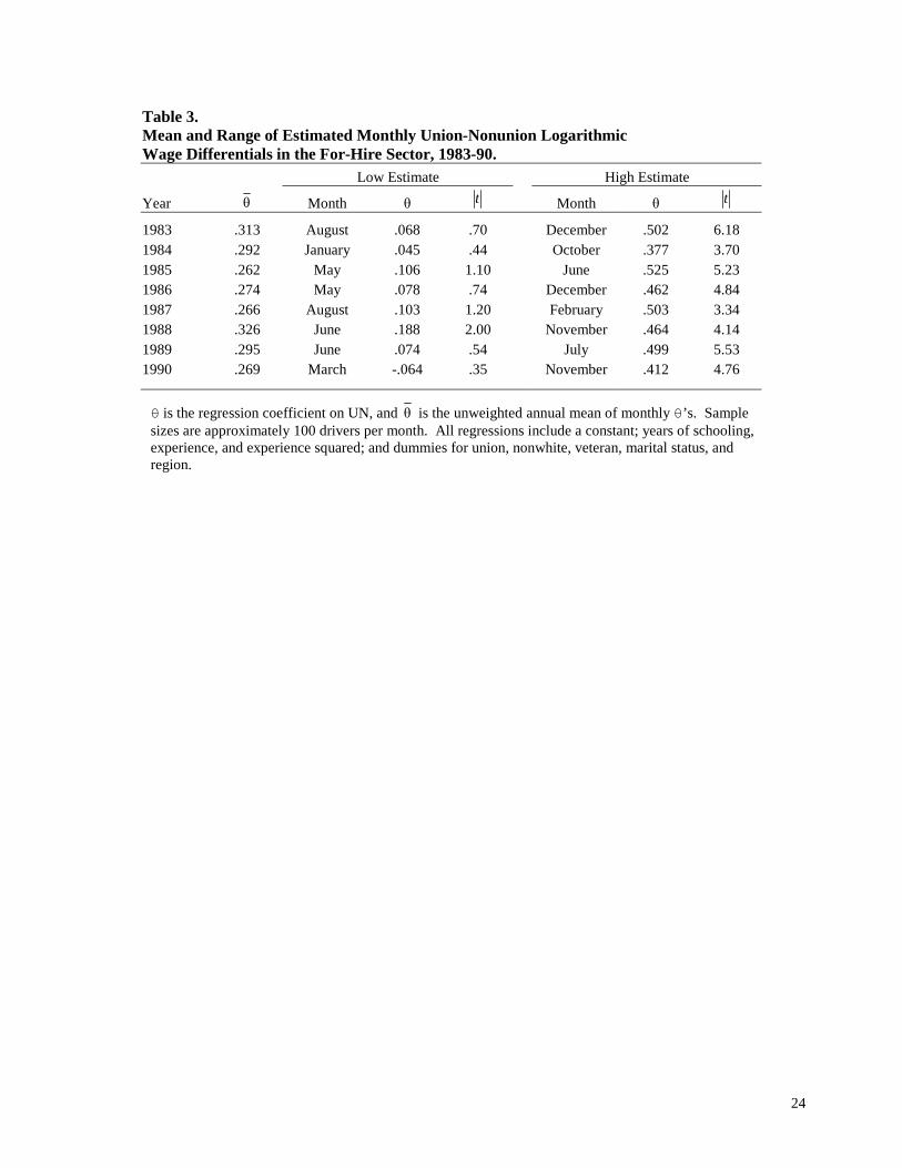
regressions in the for-hire sector are estimated for January 1983 - December 1990. Table 3 presents the

8

means (unweighted) of the monthly estimates, as well as the minimum and maximum estimates. Month-to-

month variability is found to be substantial. For example, in 1985 union premium estimates range from a

low of .106 for the May sample to a high of .525 for the December sample.7 No obvious seasonal pattern is

evident in the month-to-month variability. Rather, the results reported in Table 3 imply rather clearly that

reliable inferences cannot be drawn from regression results based on single-month samples of approximately

100 drivers, about 30 of whom are union members. Annual estimates of the union wage premium based

only on the May survey do not permit inferences as to the exact timing of the labor market responses to

deregulation. The month-to-month variability in estimates demonstrated in Table 3 does help explain the

rather weak correspondence found between contract terms in the National Master Freight Agreements and

May CPS estimates of union wage premiums during 1973-85 (see Rose, 1987; for a recent summary of

NMFA contract terms, see Bureau of National Affairs, 1991).

Finally, use of the 96 monthly CPS surveys permits analysis of male-female wage differentials, not

possible previously owing to the small number of female drivers (Rose 1987, p. 1159n). There are 444

female drivers in the combined samples for 1983-90 (and 22,496 males). Female drivers tend to be younger

(35.1 versus 38.6 years), more educated (11.7 versus 11.0 years), less likely to be married (50.2% vs.

73.0%), and less likely to be union members (15.5% vs. 29.2%) than their male counterparts. Estimation of

a pooled male-female wage equation for 1983-90 (N = 22,940) produces a coefficient (|t|) of -0.195 (11.01)

on a female dummy variable, indicating female drivers have hourly earnings 17.7% lower than similar males

(all variables are the same as in previous regressions). The unadjusted mean log wage differential is 0.244.

Estimation of the gender differential using separate male and female wage equations, and weighting

alternatively by male and female coefficients, produces virtually identical estimates. Is the estimated gender

wage gap large or small? It is low relative to economy-wide gender gaps. But much of the economy-wide

gap reflects inter-occupational differences, while gaps within narrowly-defined occupations are generally

lower than the gap among truck drivers. The CPS provides neither sufficiently detailed information on

worker and job characteristics, nor large enough samples of female drivers to permit a detailed analysis of

the determinants of the gender gap. In fact, the severely limited employment of female drivers may say

7 Note that the rather unrepresentative May 1985 survey formed the end-point used in both the Rose (1987)and Hirsch (1988) studies.

9

more about discriminatory barriers facing women than do estimates of wage differentials among existing

drivers.8

Longitudinal Analysis: Is the Union Premium a Compensating Differential?

A potential problem in previous analyses has been the inability to control for unobservable

determinants of truck driver quality. Specifically, employee and employer sorting make it likely that part of

the observed union-nonunion wage differential among drivers reflects a compensating quality premium

rather than a rent. Quality differences are most likely to arise because employers paying union wages can

select higher quality drivers from among drivers in the job queue. Quality differences might also arise

owing to lower quit rates or greater occupation- and firm-specific skills among more highly paid drivers.

Higher quality drivers also might have a greater preference for union representation and thus can be

organized at lower cost. Measured differences in years of schooling are unlikely to provide a good measure

of differences in driver quality.

In order to address the issue of unmeasured driver quality, we exploit the panel construction of the

CPS. Individuals are included in the CPS for 8 months – 4 consecutive months in the survey, followed by 8

months out, followed by 4 months in. Earnings supplement questions (weekly earnings, hours, and union

status) are asked only of the outgoing rotations (surveys 4 and 8); thus individuals provide usable

observations for the same month in consecutive years. For example, the 1989-90 panel includes male

drivers observed in their 4th survey in 1989 and 8th survey in 1990, who report their occupation as truck

driver during both years. Excluded from the 1989-90 panel are drivers in their 8th survey in 1989, their 4th

survey in 1990, workers who are drivers in 1989 or 1990 but not both, and females. Estimates in this section

are provided for 7 panels of drivers – the periods 1983-84 through 1989-90. In order to construct the panels,

drivers are identified based on household identification numbers, as well as age, survey rotation, month, and

year information.9

8 The 1979, 1983, and 1988 May/June CPS Pension Supplements, containing information on tenure with current employer, include only 13 female drivers. These women have an average ratio of years of tenure to years of potential experience of .182, as compared to .314 for male drivers (N = 1,167). 9 The Data Appendix describes construction of the longitudinal data set. Sample selection criteria are the same as previously, except drivers are required to work at least 30 hours per week in at least one rather than both years. Although correcting for some econometric problems, the subsequent analysis may introduce additional problems owing to measurement error in change variables and because changes in union status may not be independent of

10

The longitudinal samples consist of 3,659 male drivers in the for-hire and private sectors, each with

multiple observations in adjoining years. Since wage determination and union-nonunion wage differentials

are found to be broadly similar in the for-hire and private sectors following deregulation, I opt for the

efficiency gains provided by a pooled analysis of the two sectors and multiple years (a sector variable is

included). Four union states are defined: nonunion stayers (UN00), union stayers (UN11), union joiners

(UN01), and union leavers (UN10), where the first number refers to union status in year 1 and the second to

union status in year 2. Over the period approximately 9 percent of our sample changes union status during

the year, roughly half being union joiners and half leavers (measurement error in the union status variable is

discussed subsequently).

Longitudinal estimates of union wage premiums are estimated as follows. Let the wage equation in

levels, pooled across years, be:

(2) ln Wiy = αy + βXiy + τUNiy + Φi + εiy,

where ln Wiy represents the log wage of driver i in year y, vector X includes control variables and its

coefficient vector β (assumed fixed over time), αy represents regression constants allowed to vary by year, τ

represents the logarithmic union-nonunion wage premium assumed fixed over time, Φi is a driver-specific

fixed-effect constant over the 2 periods for which each driver is observed, and εiy is a random error term with

zero mean and constant variance. If the omitted fixed effect (Φi) capturing unmeasured driver skill

differences is correlated with union status, estimation of (2) in levels form will lead to biased estimates of τ.

In difference form, letting t equal panel period y minus y-1, equation (2) becomes:

(3) ∆ln Wit = ∆αt + β∆Xit + τ∆UNit + ∆εit.

In difference form, fixed effect Φi falls out, therefore purging correlation between UN and unmeasured

driver quality differences. Panel specific intercepts ∆αt capture both wage changes among drivers who do

not change union status and the effect of one additional year of experience (∆EXP = 1 for all observations,

whereas ∆EXPSQ varies with the level of EXP). The union wage premium is now estimated based on wage

changes among union status changers, where union joiners have ∆UN = 1, union leavers ∆UN = -1, and

nonunion and union stayers ∆UN = 0. The control variables in X vary little or remain fixed over a two-year

unobservables correlated with wages. For previous estimation of a wage change equation using matched CPS data, see Mellow (1981).

11

period. Nonwhite, veteran status, and region (by design of the CPS) remain fixed and fall out, while

changes in experience equal one and are reflected in the period intercepts. In addition to the change in union

status and period dummies, included explanatory variables are change variables for schooling, experience

squared, marital status, and sector (for-hire or private), and dummies for region.

Equation (3) restricts estimates of to be symmetrical such that wage gains for union joiners are

equivalent to wage losses for leavers, and assumes panel period wage changes are equivalent for nonunion

and union stayers. The following less restrictive specification relaxes these assumptions, allowing wage

changes to differ between nonunion and union stayers and different estimates of for union joiners and

leavers.

(4) ∆ln Wit = ∆αt + β∆Xit + τ01UN01it + τ10UN10it + τ11UN11it + ∆εit.

UN01, UN10, and UN11 are dummy variables set equal to 1 if the driver is a union joiner, leaver, or stayer,

respectively. The parameter τ01 provides a longitudinal estimate of the union wage premium based on the

sample of union joiners, compared to the base group of nonunion stayers; -( τ10- τ11) provides an alternative

estimate of the union premium based on the sample of union leavers, compared to the group of union

stayers. Separate annual estimates of τ01, τ10, and τ11 are possible, but entail considerable loss in efficiency

and a high variability in estimates owing to the small number of union joiners and leavers in each panel.

Table 4 provides regression results for the longitudinal sample of 3,654 drivers, each observed in

consecutive years (the periods 1983-84 through 1989-90). Three sets of union premium estimates are

presented. The first column presents a 1984-90 premium estimate based on a wage levels equation whose

observations are the second year for each driver; the second column presents a longitudinal estimate based

on the coefficient of ∆UN in a wage change equation (eq. 3), thus restricting the estimated premium to be

equivalent for joiners and leavers; and the third column presents alternative longitudinal estimates based

separately on union joiners and leavers (eq. 4). The levels equation includes the same set of control

variables included previously, plus year dummies. The wage change equations include variables measuring

changes in schooling, experience squared, marital status, and sector, as well as dummies for period and

region (the union coefficients are invariant to inclusion of the dummies). The control variables provide

12

virtually no explanatory power. And as seen by the low R2s in the change equations, union status change

(not surprisingly) explains a tiny portion of the year-to-year change in individual wages.

The estimate of the 1984-90 union premium for this sample of drivers, based on the levels equation

shown in the first column, is 0.279 (|t| = 22.05), consistent with evidence presented in Table 1. Longitudinal

estimates of the union premium are substantially lower. The wage change results presented in the second

column provide a union premium estimate of only 0.049 (2.51), about a sixth as large as the levels estimate.

The less restrictive specification in column three permitting alternative estimates of the union premium

based on union joiners and leavers, τ01 and -(τ10 - τ11), respectively, produces estimates of 0.051 (1.74) for

joiners and .053 (1.82) for leavers.

In levels analysis not shown, union joiners are found to earn more than nonunion drivers even in the

initial year when both are nonunion, and union leavers are found to earn more than nonunion drivers in the

second year when both are nonunion. These results, along with the longitudinal estimates presented in

Table 4, are consistent with the existence of a queue of qualified drivers for union jobs, with those selected

being more able than the average nonunion driver.

How much of the union wage advantage represents a rent, and how much is a compensating

premium for labor quality? There is no unique decomposition of the union-nonunion wage differential into

quality and rent components. But if it is assumed that there is no measurement error and that union status

change is exogenous, or more specifically, that drivers who are union members for either or both of the

years have homogeneous labor quality for given measured characteristics (other than union status), such a

division can be approximated by comparing the union premiums estimated above for joiners and leavers, to

the observed differential in the levels equation.10 Let 0.053 be our best estimate of the longitudinal union

premium, based on the average of the estimated wage premium for union joiners and leavers in equation 3.

This is only 19% of the observed levels premium (.053/.279=.190). Thus, the estimates imply that much of

10 The direction of bias is indeterminate if union status change is endogenous. For example, if union leavers voluntarily leave union for nonunion jobs, there will be a downward bias in the union premium estimate for leavers since unusually high wage opportunities increase the probability of voluntary job change. However, involuntary union job loss is likely among drivers in companies with particularly high wage scales, leading to estimates of bias in the opposite direction since these drivers would experience unusually large wage decreases.

13

the observed union-nonunion wage differential observed for truck drivers is not a rent but, rather, reflects a

compensating premium for driver quality.

As is widely recognized (e.g., Freeman 1984; Griliches and Hausman 1986; Card 1991),

measurement error in the union variable can cause substantial downward bias in longitudinal estimates of

the union premium; the bias be larger the smaller the number of union changers and the larger the proportion

of the sample with incorrectly classified union status. There are two principal sources of measurement error

in the union variable – inaccurate answers given by survey respondents or recording errors by the Census,

and incorrect allocations by the Census among workers without responses to the union question. The

proportion of inaccurate responses or recording errors on the union question is reasonably small (2.5%-

3.0%) and has little effect on levels estimates of the union premium (Mellow and Sider 1983; Card 1991).

Its effect on the magnitude of longitudinal estimates is less certain but can be substantial. Freeman (1984)

provides a range of estimates, but assumes that matched firm records are accurate (see Card, 1991, on this

issue) and does not account for the fact that serially correlated measurement error lessens the downward bias

(for analysis of this issue, see Bound and Krueger, 1991). Measurement error is increased here by focusing

on a single occupation, since occupational mobility is a source for some of the true variation in union status,

and by use of brief two-year periods, since the noise-to-signal ratio is higher the shorter the time period. On

the other hand, driving skills are largely occupation rather than firm specific, so drivers can change

employers and union status without changing occupation. Unknown is whether truck drivers are more or

less likely than are average workers to report incorrectly their union status.

Approximately 2% of workers have their union status allocated by the Census through a matching of

non-respondents to responding workers with similar characteristics. Among the sample of union status

changers, a higher proportion will have had their union status allocated, since an incorrect allocation is

likely to produce a measured changer. Unfortunately, the allocation flag indicating whether union status is

allocated is not contained on the 1983-88 microdata earnings file tapes provided to the BLS by the Census;

they are available beginning in 1989. How serious is the measurement error and bias resulting from

incorrect Census allocations? We are not sure. Examining the 1989-90 panel, 16% (8 out of 50) of the

union joiners and leavers had their union status allocated in either 1989 or 1990. Longitudinal union

14

premium estimates for the 1989-90 panel, however, are similar in change equations with and without the

workers whose status is allocated in at least one of the years (the coefficients on ∆UN are .118 and .114,

respectively). Separate estimates for joiners and leavers are not symmetric in the 1989-90 sample and

display greater sensitivity to exclusion of drivers with allocated union status.11

Although the seriousness of measurement error in the union change variable cannot be known with

certainty, the large difference in estimates between the longitudinal and levels equations (.053 vs. .279)

makes us confident that a substantial portion (half may be a good guesstimate) of the union-nonunion

differential for truck drivers is a compensating quality premium. For example, suppose that measurement

error is so severe that longitudinal estimates of the quality-adjusted union premium are biased downward to

a third of their true value. Even then, over 40% of the estimated cross-section union-nonunion wage

differential (already adjusted for measurable wage determinants) can be attributed to unmeasured quality

differences (1 - [(3 x .053)/.279] = .430). The results support the expectation that employers offset some of

the union-nonunion wage differential through selective hiring; both driver quality and wages are higher than

they would be absent unionization. Although the pure rents accruing to unionized truck drivers cannot be

estimated with accuracy, the continuing decline in union density during 1983-90 suggests that these rents

remain substantial.

The previous longitudinal analysis examined wage changes among workers who are truck drivers in

adjacent years. The data set also allows an examination of wage changes among workers changing

occupations – from truck driver in year 1 to another occupation, or from another occupation in year 1 to

driver in year 2. Such a sample is constructed using the same sampling criteria used to construct the

previous panel of drivers. Estimates from this sample allow measurement of the gains and losses associated

with changes into and out of both truck driving and union membership.

The CPS earnings files for 1983-90 allow construction of a panel of 1,473 workers who are truck

drivers in year 1 (survey rotation 4) and not in year 2 (rotation 8), and of 1,580 workers who are not drivers

11 Prior to going to press, I examined the 1991 CPS earnings files and constructed a 1990-91 panel of drivers. The panel contains 57 union changers, 11 of whom had union status allocated in at least one of the years. Estimates from change equations including and excluding drivers with allocated status, using the combined 1989-90 and 1990-91 panels, produce coefficients on ∆UN of .122 and .104, respectively. This limited evidence does not indicate any downward bias in longitudinal estimates arising from the Census allocation of union status.

15

in year 1 and are in year 2. In both samples, about 12% have changed union status, with roughly an even

split between joiners and leavers. Preliminary analysis (not shown) indicated that for both samples of

workers, union premium estimates based alternatively on union joiners and leavers are highly similar. For

ease of exposition, results therefore are presented using a specification with the ∆UN variable and for a

panel (N = 6,712) pooling the three longitudinal samples: truck drivers in adjacent years (TT = 1, N =

3,659), drivers in year 1 and not in year 2 (TN = 1, N = 1,473), and not a driver in year 1 and a driver in year

2 (NT = 1, N = 1,580). The following regression results are obtained from a wage change equation for the

combined 1983-84 through 1989-90 panels (|t| in parentheses):

∆ ln Wt = .001TN - .005NT + .048TT∆UN + .131TNDUN + .116NT∆UN, N = 6,712 R2 = 0.016

(0.10) (0.43) (2.34) (4.59) (4.25)

The wage change regression also includes variables measuring changes in schooling, experience squared,

marital status, and presence in the for-hire trucking sector, as well as dummies for region and period. The

omitted reference group represents individuals who are truck drivers in both years (TT = 1). The absence of

wage gains or losses associated with leaving or entering truck driving (the coefficients on TN and NT,

respectively) is of interest. Small gains or losses associated with occupational change could reflect

relatively low (i.e., quickly learned) investment in training by drivers. Alternatively, the loss in human

capital resulting from occupational change could be substantial since driving skills are to a considerable

degree occupation specific, but this loss may be offset by gains associated with voluntary (i.e., non-random)

job change.

The estimated longitudinal union premium for the trucker-trucker sample of drivers is about 5%, as

seen previously in Table 4. But for the samples of drivers changing occupation, estimated wage changes

associated with the change in union status are 12%-14%. Although higher than the estimate from the TT

sample (perhaps due in part to lower measurement error bias among occupation changers), the longitudinal

premiums remain far lower than estimates of the differential in levels, which are approximately .30 for all

three groups of workers (levels results for the occupational changers are not shown). Although the exact

magnitude of the union premium associated with union status change is again in doubt, the large difference

16

in premium estimates between the levels and change equations make us confident that much of the observed

union-nonunion wage differential in fact reflects labor quality differences in drivers.

Interpretation and Conclusions

Deregulation in the trucking industry provides an unusually rich opportunity to study the creation

and dissolution of economic rents associated with entry, price, and operating restrictions. Past studies have

provided strong evidence that rents arising from regulation were reflected not only in higher profitability and

in the market value of operating rights, but also in the form of higher labor costs. Previous analyses,

however, were limited by small sample sizes of truck drivers, and the concomitant high variability of

estimates, during the post-regulation period. This paper examines wage determination among truck drivers

using the 96 monthly samples from the Current Population Surveys for 1983-90, thus facilitating more

current and precise estimation of union density and union-nonunion wage differentials during the

deregulatory period, as well as the use of longitudinal analysis to examine wage changes for union joiners

and leavers.

The evidence is broadly supportive of the conclusions reached previously by Rose and Hirsch. In

the previously regulated for-hire sector of the trucking industry, union density fell continuously from about

60% during the regulatory period to about 25% by 1990. Union-nonunion wage differentials (in log

differences) fell from about 0.40 during 1973-78 to a range of .26-.33 during 1983-90. Union-nonunion

wage differentials among drivers in the unregulated private carrier sector were about 0.30 during the earlier

period, but have fallen little during the 1980s and are roughly similar in magnitude to union premiums in the

for-hire sector.

Longitudinal analysis is performed on seven panels of truck drivers for whom data are available for

1983-84 through 1989-90. Wage changes among union joiners and leavers allow inferences to be made

about unmeasured quality differences between union and nonunion drivers. Union premium estimates based

on longitudinal data are considerably lower than are union-nonunion differentials estimated from levels data.

Based on results from the panel data, we conclude that a substantial portion of the union-nonunion wage

differential is a compensating premium for unmeasured driver quality, consistent with the hypothesis that

union employers select and retain relatively high-quality drivers.

17

Data from supplemental sources also is examined to shed further light on this paper's results.

Corroborative evidence on unionization and wages among truck drivers is available in private surveys of

long-haul truckload (TL) drivers in 1980 and 1987.12 The National Motor Transportation Data Base

contains survey data collected from drivers at 20 U.S. truckstop sites, with approximately 17,000

observations in 1980 and 19,000 in 1987. These surveys do not sample a representative cross-section of

drivers but, rather, a fairly narrow segment of the total universe of drivers. The survey primarily includes

long-haul truckload drivers along major long-haul (rail competitive) corridors, a large proportion of whom

are involved in irregular-route common carriage. The survey largely excludes short-haul TL drivers who

generally run on a straight through nonstop schedule, and drivers in the highly unionized less-than-truckload

(LTL) segment who drive terminal to terminal.

Union density among those drivers surveyed (primarily for-hire TL) fell sharply during the

deregulation period, from 19.4% in 1980 to only 2.6% in 1987 (coverage among the tiny regular-route LTL

common carriage component of this sample fell from 74.4% to 56.4% during this period). The cost

differential between union and nonunion trucking has exhibited little change during the period. Estimated

costs per mile were 22.3% higher among union than nonunion trucking in 1987, as compared to 20.5%in

1980. Consistent with our finding that part of the union wage premium reflects a quality differential, the

survey finds that union drivers are older, have more trucking experience, and have greater tenure with their

present firm than do nonunion drivers. Moreover, the gap between union and nonunion drivers in these

three characteristics widened between 1980 and 1987.

The relationship between truck drivers’ union status and job tenure also is explored more fully using

the CPS Pension Supplements attaching to the 1979, 1983, and 1988 May/June public use tapes. The

Supplements include a question asking number of years with the current employer. Comparison of union

and nonunion years of tenure may be a reasonable proxy for relative years of driver experience.13 Taking

the ratio of years of tenure on current job to years of potential experience (age-schooling-5), we obtain a

12 Information on these surveys has been kindly provided and summarized by William Linde, Intermodal Policy Division, American Association of Railroads. 13 Union workers generally have lower permanent turnover rates than do nonunion workers. If, on the one hand, this generalization is also correct for truck drivers, the ratio of tenure to years of total driver experience will be higher for union than for nonunion drivers. On the other hand, the business failure of numerous union trucking operations during the 1980s would lead to a bias in the opposite direction.

18

value of .383 for male union drivers in the combined 1979, 1983, and 1988 Pension Supplements, as

compared to only .277 for the sample of nonunion drivers. In 1988 union drivers averaged 10.95 years of

tenure on the current job and 25.76 years of potential experience. The comparable figures for nonunion

drivers are 5.17 years of tenure and 20.44 years of potential experience. The tenure-experience ratio

exhibited a small increase among union drivers between 1979 and 1988, while showing little change among

nonunion drivers. The tenure results reinforce and help explain the earlier finding that a substantial portion

of the union-nonunion wage differential appears to be a compensating premium for higher quality. Union

drivers possess greater tenure and (by inference) driving experience than do nonunion drivers of similar age.

Deregulation in the trucking industry has limited the ability of firms to continue maintenance of

costly unionized trucking operations, except where high wages can be offset by productivity advantages or

where union operations are partially protected from nonunion competition as is the case in many LTL

markets. Evidence from the CPS indicates that the cost pressures brought to bear upon union wages have

produced a narrowing in what once was a very large union-nonunion wage differential in the for-hire sector

of the industry. For the Teamsters to have maintained union density at levels obtained during the regulatory

period, however, the union would have had to agree to wage and benefit concessions far greater than they

did. Evidence clearly indicates that the rank-and-file were unwilling to support many of the concessions

actually recommended by the Teamster leadership, while the even greater concessions that were necessary

to protect employment of union drivers were not politically feasible. Currently, the trucking industry is

characterized by a union sector much smaller than during the regulatory period and in which union drivers

continue to realize a sizable albeit reduced wage premium, a portion of which is offset by higher quality

among union drivers.

19

Data Appendix: Construction of the Longitudinal Sample from the CPS Outgoing Rotation Files

Households are included in the CPS for 8 months – 4 consecutive months in the survey, followed by

8 months out, followed by 4 months in. The CPS contains household identification numbers (ID), but not

individual identifiers. Since January 1983, the CPS has included the earnings supplement questions (weekly

earnings, hours, union status, etc.) each month, rather than just in the May surveys. But only the outgoing

rotation groups 4 and 8 are asked these questions. Individuals potentially can be identified for the same

month in consecutive years; that is, individuals in rotation 4 in year 1 can be matched to individuals in

rotation 8 in year 2. The CPS ran a test sample from July-September 1985 in order to implement new

population weights and area identifiers. As a result, rotation 4 households interviewed in July 1984 through

September 1985 were not reinterviewed a year later in 1985 and 1986. Therefore, the longitudinal sample

for 1984-85 is approximately one-half, and the sample for 1985-86 approximately one-quarter, the normal

size.

The longitudinal file was created in the following manner. Separate data files were created

separately for males and females, and for pairs of years (rotation 4 1983, and rotation 8, 1984; rotation 4,

1984, and rotation 8, 1985; etc.). Within each file, individuals were sorted as appropriate on the basis of

ascending and descending household ID, year, and age. To be considered an acceptable matched pair, a

rotation 8 individual had to be matched with a rotation 4 individual with identical household ID, identical

survey month, and an age difference between 0 and 2 (since surveys can occur on different days of the

month, age change need not equal 1). Several passes were necessary because a single household may

contain more than one male or female pair. Checks were provided to insure that only unique matches were

selected. For each rotation 8 individual, the search was made through all rotation 4 individuals with the

same ID to make sure there was only 1 possible match; the file was resorted in reverse order and each

selected rotation 4 individual was checked to insure a unique rotation 8 match. As uniquely matched pairs

were identified they were removed from the work file. Incorrect changes in the variables marital status,

veteran status, race, and education (e.g., a change in schooling other than 0 or 1, a change from married to

never married, etc.) were used to delete “bad” observations in households where there were multiple

observations and ages too close to separate matched pairs. Several passes at the data were made. In

20

households where two pairs of individuals could be separated based on a 1 year but not the 0 to 2 year age

change, a 1 year criterion was used. If a unique pair could not be identified based on these criteria, they

were not included in the data set (e.g., four observations with two identical pairs, or three individuals with

two possible matches using the 0 to 2 age change criterion).

The match rate in the longitudinal analysis is 64%. A match rate of 64.3% is obtained based on the

percentage of the 7,883 rotation 4 truckers for 1983-89 included in the levels analysis (this excludes

observations during July 1984 - September 1985 for reasons stated above) who also are included in the

subsequent longitudinal analysis – 5,068 rotation 8 workers in the trucker-trucker and trucker-nontrucker

samples during 1984-90 (the combined TT and TN samples shown in the text were N = 5,132 and included

workers with 30 or more hours in at least one of the years; 64 of these had fewer than 30 hours in year 1 and

were not included in the levels analysis or the calculation of the match rate). Alternatively, a match rate of

64.4% is obtained based on the percentage of the 8,066 rotation 8 truckers for 1984-90 included in the levels

analysis who also are included in the longitudinal analysis – 5,191 rotation 4 workers in the trucker-trucker

and nontrucker-trucker samples during 1983-89. The principal reasons that matches cannot be made are if a

household moves (thus changing the household ID), if an individual moves out of a household (young

workers are less likely to be matched), if an individual drops out of the labor market or fails to meet other

sample selection criteria, or if the Census is unable to reinterview a household and/or receive information on

the individual. Note that the match rate reported here is similar to the match rate of 68.8% for the 1987-88

CPS reported by Card (1991) using a broader-based sample and a less stringent probabilistic matching

algorithm obtained from the Bureau of Labor Statistics.

21

References

Bound, John and Krueger, Alan B. “The Extent of Measurement Error in Longitudinal Earnings Data: Do

Two Wrongs Make a Right?” Journal of Labor Economics 9 (January 1991): 1-24.

Bureau of National Affairs. Collective Bargaining Negotiations and Contracts. Washington: BNA, May 30,

1991.

Card, David. “Deregulation and Labor Earnings in the Airline Industry.” Industrial Relations Section

Working Paper #247, Princeton University, January 1989.

Card, David. “The Effect of Unions on the Distribution of Wages: Redistribution or Relabelling?”

Industrial Relations Section Working Paper #287, Princeton University, July 1991.

Freeman, Richard B. “Longitudinal Analyses of the Effects of Trade Unions.” Journal of Labor Economics

2 (January 1984): 1-26.

Giles, David E. A. “The Interpretation of Dummy Variables in Semilogarithmic Equations: Unbiased

Estimation.” Economics Letters 10 (1982): 77-79.

Griliches, Zvi and Hausman, Jerry. “Errors in Variables in Panel Data.” Journal of Econometrics 31

(February 1986): 93-118.

Hirsch, Barry T. “Trucking Regulation, Unionization, and Labor Earnings: 1973-85.” Journal of Human

Resources 23 (Summer 1988): 296-319.

Hirsch, Barry T., and Addison, John T. The Economic Analysis of Unions: New Approaches and Evidence.

Boston: Allen & Unwin, 1986.

Lazear, Edward P. “A Competitive Theory of Monopoly Unionism.” American Economic Review 73

(September 1983): 631-43.

Lewis, H. Gregg. Union Relative Wage Effects: A Survey. Chicago: University of Chicago Press, 1986.

Mellow, Wesley. “Unionism and Wages: A Longitudinal Analysis.” Review of Economics and Statistics

63 (February 1981): 43-52.

Mellow, Wesley and Sider, Hal. “Accuracy of Response in Labor Market Surveys: Evidence and

Implications.” Journal of Labor Economics 1 (October 1983): 331-44

Rose, Nancy L. “The Incidence of Regulatory Rents in the Motor Carrier Industry.” Rand Journal of

Economics 16 (Autumn 1985): 299-318.

_______. “Labor Rent-Sharing and Regulation: Evidence from the Trucking Industry.” Journal of

Political Economy 95 (December 1987): 1146-78.

Ying, John S. and Keeler, Theodore E. “Pricing in a Deregulated Environment: The Motor Carrier

Experience.” Rand Journal of Economics 22 (Summer 1991): 264-73.

22

Table 1. Mean Real Wages, Union Density, and Union Wage Premium Estimates for Male Truck Drivers, 1973-90

Drivers in For-Hire Sector Drivers in Private Carrier Sector

N DEN Wu Wn ln Wu – ln Wn θ t N DEN Wu Wn ln Wu – ln Wn θ t

A. Using only May public use CPS samples:

1973-78 1,533 .599 15.76 10.68 .452 .392 19.24 3,170 .364 13.25 9.00 .403 .300 23.18 1979a 175 .566 14.86 11.31 .308 .244 3.87 338 .352 13.37 9.44 .368 .248 5.73 1980a 94 .564 13.91 10.69 .245 .156 1.64 213 .423 12.69 9.13 .355 .281 5.60 1981a 84 .607 14.69 11.75 .214 .170 2.02 176 .364 13.03 9.63 .294 .202 2.96 1983a 127 .504 14.35 10.07 .363 .324 5.26 248 .343 12.58 9.20 .293 .229 4.09 1984a 79 .304 14.36 10.18 .366 .360 4.02 145 .290 12.84 9.45 .342 .277 4.09 1985a 111 .288 12.43 10.59 .205 .106 1.10 156 .288 14.58 8.82 .541 .403 6.55

B. Using all 12 monthly CPS samples for each year:

1983 1,034 .432 14.70 10.45 .370 .311 11.60 1,867 .312 13.03 9.16 .374 .291 15.22 1984 1,158 .375 14.12 10.72 .314 .282 10.70 1,854 .286 12.87 9.09 .364 .288 15.18 1985 1,154 .341 13.83 10.47 .299 .260 10.24 1,744 .287 13.31 9.12 .409 .300 15.11 1986 1,093 .319 14.00 10.39 .347 .293 11.11 1,683 .269 13.06 9.04 .390 .305 15.37 1987 1,136 .276 13.49 10.00 .337 .269 9.89 1,599 .283 12.95 9.13 .359 .275 13.64 1988 1,161 .300 13.84 9.84 .365 .328 12.25 1,448 .256 12.62 9.01 .360 .254 11.66 1989 1,166 .269 13.64 9.88 .350 .307 10.67 1,565 .247 12.94 8.92 .394 .299 13.32 1990 1,264 .241 13.68 10.21 .333 .283 10.39 1,570 .249 12.29 8.90 .334 .250 11.43

Source: for panel A: Hirsch (1988). CPS = Current Population Survey; DEN = union density, W = usual weekly earnings divided by usual hours worked (in 1990:4 dollars, adjusted by the quarterly Personal Consumption Expenditure component of the GNP implicit price deflator); ln Wu - ln Wn represents the unadjusted log wage differential between union and nonunion drivers; and θ represents the regression coefficient on the union membership dummy variable UN for the corresponding period. All regressions include a constant; years of schooling, experience, and experience squared; and dummies for union, nonwhite, veteran, marital status, and region (8).

23

Table 2. Mean Real Wages, Union Density, and Union Wage Premium Estimates for Male Nontruck Operatives and Blue-Collar Manufacturing Workers, 1983-90

Nontruck Operatives Blue-Collar Manufacturing Workers

N DEN Wu Wn ln Wu – ln Wn θ t N DEN Wu Wn ln Wu – ln Wn θ t

1983 7,877 .419 13.11 9.43 .374 .279 31.71 14,915 .429 13.17 10.97 .225 .146 24.78 1984 8,191 .400 12.98 9.34 .366 .266 31.71 15,534 .407 13.08 10.81 .236 .150 25.75 1985 8,267 .389 13.16 9.31 .385 .295 33.96 15,415 .388 13.26 10.91 .241 .158 26.39 1986 7,884 .377 13.13 9.40 .384 .279 28.35 14,926 .374 13.33 10.82 .255 .171 27.71 1987 7,735 .348 12.98 9.08 .400 .284 29.18 14,739 .362 13.04 10.55 .256 .158 24.91 1988 7,276 .342 12.73 8.97 .385 .270 27.51 14,080 .351 12.86 10.45 .249 .150 23.17 1989 7,452 .324 12.82 9.18 .374 .266 26.15 14,308 .339 12.89 10.65 .232 .142 21.73 1990 7,742 .312 12.60 9.09 .365 .255 25.99 14,403 .329 12.67 10.38 .239 .145 22.07

The data are derived from the earnings microdata files from BLS containing the 12 monthly CPS surveys. N = sample size; DEN = union density, W = usual weekly earnings divided by usual hours worked (in 1990:4 dollars, adjusted by the quarterly Personal Consumption Expenditure component of the GNP implicit price deflator); ln Wu –ln Wn represents the unadjusted log wage differential; and h represents the regression coefficient on a union membership dummy variable UN for the corresponding period. All regressions include a constant; years of schooling, experience, and experience squared; and dummies for union, nonwhite, veteran, marital status, and region (8).

24

Table 3. Mean and Range of Estimated Monthly Union-Nonunion Logarithmic Wage Differentials in the For-Hire Sector, 1983-90. Low Estimate High Estimate

Year θ Month θ t Month θ t

1983 .313 August .068 .70 December .502 6.18 1984 .292 January .045 .44 October .377 3.70 1985 .262 May .106 1.10 June .525 5.23 1986 .274 May .078 .74 December .462 4.84 1987 .266 August .103 1.20 February .503 3.34 1988 .326 June .188 2.00 November .464 4.14 1989 .295 June .074 .54 July .499 5.53 1990 .269 March -.064 .35 November .412 4.76

θ is the regression coefficient on UN, and θ is the unweighted annual mean of monthly θ’s. Sample sizes are approximately 100 drivers per month. All regressions include a constant; years of schooling, experience, and experience squared; and dummies for union, nonwhite, veteran, marital status, and region.

25

Table 4. Longitudinal Analysis of Union Wage Effects, Combined Panels for 1983-84 through 1989-90. Dependent Variable

Union (Variable) Mean ln W ∆ ln W ∆ ln W

Union Membership .350 .278 – – (UN) (22.05) Change in UN -.004 – .049 – DUN (2.51) Union joiner .044 – – .051 UN01 (1.74) Union leaver .048 – – -.047 UN10 (1.66) Union stayer .306 – – .006 UN11 (.45) Nonunion stayer .602 – – – UN00 R2 .255 .007 .007 N 3,659 3,659 3,659

The first regression is a levels equation with second-year observations for each driver and ln W as the dependent variable; included variables are years of schooling, experience, and experience squared; and dummies for union, nonwhite, veteran, marital status, trucking sector, region, and year. The second and third regressions are wage change equations with ∆ ln W the dependent variable (mean equals .013), corresponding to equations (3) and (4) in the text. Included variables are changes in schooling, experience squared, marital status, and sector, and dummies for region and 2 panel year periods. Nonunion stayer (UN00) is the omitted category in the third column. t is given in parentheses.