Tropospheric stability at candidate SKA sites 1 · PDF fileWordprocessor MsWord Word 2007...

Name Designation

R P Millenaar Chief Site

Engineer

R T Schilizzi Director

R T Schilizzi Director

TROPOSPHERIC STABILI

Document number ................................

Revision ................................

Author ................................

Date ................................................................

Status ................................................................

Affiliation Date

Submitted by:

SPDO 02/11/11

Accepted by:

SPDO 02/11/11

Approved by:

SPDO 02/11/11

TROPOSPHERIC STABILITY AT CANDIDATE SKA

...................................................................WP3-040.020.001

...........................................................................................................................

.........................................................................................................

...................................................................................

..................................................................... Final

Signature

TY AT CANDIDATE SKA SITES

040.020.001-TR-001

........................... A

......... R.P. Millenaar

................... 2-11-2011

Final Confidential

WP3-040.020.001-TR-001

Revision : A

of 55

DOCUMENT HISTORY

Revision Date Of Issue Engineering Change

Number

Comments

- 25-10-2011 - first draft

A 2-11-2011 - final

DOCUMENT SOFTWARE

Package Version Filename

Wordprocessor MsWord Word 2007 Tropospheric stability at candidate SKA sites 1.0.docx

Block diagrams

Other

ORGANISATION DETAILS Name SKA Program Development Office

Physical/Postal

Address

Jodrell Bank Centre for Astrophysics

Alan Turing Building

The University of Manchester

Oxford Road

Manchester, UK

M13 9PL

Fax. +44 (0)161 275 4049

Website www.skatelescope.org

WP3-040.020.001-TR-001

Revision : A

of 55

TABLE OF CONTENTS

1 INTRODUCTION ............................................................................................. 6

2 SCOPE ......................................................................................................... 6

3 ORGANISATION OF WORK ................................................................................ 6

3.1 Partners and responsibilities ..................................................................................................... 6

3.2 Installation and commissioning ................................................................................................. 7

4 PROCESSING PRINCIPLES .................................................................................. 7

5 SITE DESCRIPTIONS ......................................................................................... 9

5.1 Boolardy, Australia .................................................................................................................... 9

5.2 Karoo, South Africa .................................................................................................................. 11

6 RESULTS .................................................................................................... 13

6.1 Measurement period ............................................................................................................... 13

6.1.1 Overview of measurements Australia .............................................................................. 14

6.1.2 Overview of measurements South Africa ......................................................................... 16

6.2 Tropospheric delay data .......................................................................................................... 20

6.2.1 Delay time series .............................................................................................................. 20

6.2.2 Delay cumulative distribution .......................................................................................... 20

6.2.3 Results Australia ............................................................................................................... 22

6.2.3.1 Delay time series ....................................................................................................... 22

6.2.3.2 Delay cumulative distribution ................................................................................... 28

6.2.4 Results South Africa .......................................................................................................... 31

6.2.4.1 Delay time series ....................................................................................................... 31

6.2.4.2 Delay cumulative distribution ................................................................................... 43

6.2.5 Comparisons between sites ............................................................................................. 50

7 REFERENCES ............................................................................................... 55

WP3-040.020.001-TR-001

Revision : A

of 55

FIGURES Figure 1: One of the STI dishes (West) during installation at the Australian core site ......................... 10

Figure 2: One of the dishes (West) at the South African core site ....................................................... 12

Figure 3: Overview Australia June 2011 ................................................................................................ 14

Figure 4: Overview Australia July 2011 ................................................................................................. 14

Figure 5: Overview Australia August 2011 ............................................................................................ 14

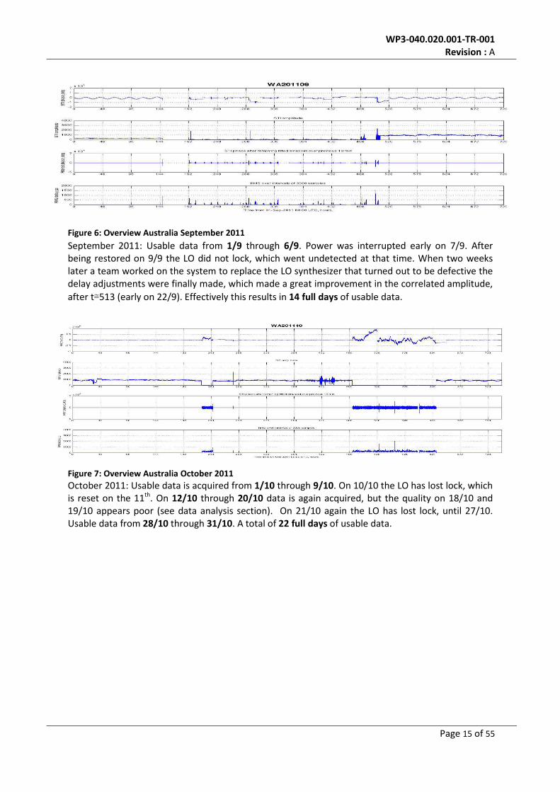
Figure 7: Overview Australia October 2011 .......................................................................................... 15

Figure 6: Overview Australia September 2011 ..................................................................................... 15

Figure 8: Overview South Africa March 2011 ....................................................................................... 16

Figure 9: Overview South Africa April 2011 .......................................................................................... 16

Figure 10: Overview South Africa May 2011 ........................................................................................ 16

Figure 11: Overview South Africa June 2011 ........................................................................................ 17

Figure 12: Overview South Africa July 2011 ......................................................................................... 17

Figure 13: Overview South Africa August 2011 .................................................................................... 17

Figure 14: Overview South Africa September 2011 .............................................................................. 19

Figure 15: Overview South Africa October 2011 .................................................................................. 19

Figure 16: Time series Australia June 2011 ........................................................................................... 21

Figure 17: Time series Australia July 2011 ............................................................................................ 22

Figure 18: Time series Australia August 2011 ....................................................................................... 23

Figure 19: Time series Australia September 2011 ................................................................................ 24

Figure 20: Time series Australia October 2011 ..................................................................................... 26

Figure 21: Time series Australia, zoomed-in on 18 and 19-10-2011 .................................................... 27

Figure 22: Cumulative distribution Australia June 2011 ....................................................................... 27

Figure 23: Cumulative distribution Australia August 2011 ................................................................... 28

Figure 24: Cumulative distribution Australia July 2011 ........................................................................ 28

Figure 26: Cumulative distribution Australia October 2011 ................................................................. 30

Figure 25: Cumulative distribution Australia September 2011 ............................................................ 29

Figure 27: Time series South Africa March 2011 .................................................................................. 30

Figure 28: Time series South Africa April 2011 ..................................................................................... 31

Figure 29: Time series South Africa, zoomed-in on 19-4-2011 ............................................................. 32

Figure 30: Time series South Africa May 2011 ..................................................................................... 33

Figure 31: Time series South Africa, zoomed-in on 4-5-2011 to 6-5-2011 ........................................... 34

Figure 32: Time series South Africa June 2011 ..................................................................................... 35

Figure 33: Time series South Africa July 2011 ...................................................................................... 36

Figure 34: Time series South Africa August 2011 ................................................................................. 37

Figure 35: Time series South Africa September 2011 ........................................................................... 38

Figure 36: Time series South Africa, zoomed-in on 7-09-2011 ............................................................. 41

Figure 37: Time series South Africa October 2011 ............................................................................... 42

Figure 38: Cumulative distribution South Africa March 2011 .............................................................. 41

Figure 39: Cumulative distribution South Africa April 2011 ................................................................. 42

Figure 40: Cumulative distribution South Africa May 2011 .................................................................. 42

Figure 42: Cumulative distribution South Africa July 2011 ................................................................... 47

Figure 41: Cumulative distribution South Africa June 2011 ................................................................. 43

Figure 43: Cumulative distribution South Africa August 2011 ............................................................. 47

Figure 44: Cumulative distribution South Africa September 2011 ....................................................... 48

Figure 45: Cumulative distribution South Africa October 2011............................................................ 49

Figure 46: Median rms delay over time (overall, daytime and night-time) .......................................... 50

Figure 47: Combined cumulative distribution 201106 (blue Aus, red SA) ............................................ 52



WP3-040.020.001-TR-001

Revision : A

of 55



TABLES Table 1: STI information Australia ........................................................................................................... 9

Table 2: STI information South Africa ................................................................................................... 11

Table 3: Cumulative Distribution Statistics over time .......................................................................... 51

Glossary

IEAC International Engineering Advisory Committee

RFI Radio Frequency Interference

SKA Square Kilometre Array

SPDO SKA Program Development Office

SSEC SKA Science and Engineering Committee

WP3-040.020.001-TR-001

Revision : A

of 55

1 Introduction

The tropospheric stability over the proposed core locations in the two candidate host countries,

Australia and South Africa, has been investigated. This work was organised and partly carried out by

the SPDO, within PrepSKA Work Package 3.4, which aimed to “Carry out studies of the effects of

tropospheric turbulence on high frequency observations. Study the high-frequency limits of phase-

referencing and self-calibration, and determine the implications for the SKA design” [1]. On advise

from the IEAC and SSEC the work has been carried out as in-situ measurements of tropospheric

stability. The current document reports on the measurement campaign, the instrumentation,

deployment and measurement results up to a point in time as late as practically possible. The latter

remark refers to the limited time that the measurement systems have been producing data, in

particular the one in Australia. This report therefore will be issued as close to the set delivery time as

possible, and will be revised when new data has been analysed at later dates. The document history

table will account for these updates.

In this report the candidate sites are listed in alphabetical order (Australia/Australasia before

South/Southern Africa).

2 Scope

Site Test Interferometers (STI) have been installed at the core locations of the candidate SKA hosts

and measurements were taken. The purpose is to characterise the tropospheric stability conditions

over these sites for a period long enough such that representative information is obtained, sampling

all seasons. Because of slow deployment the measurement period has been limited, to the extent

that summer months have not been observed within the available time. This report provides general

information on the systems and details the properties of the two sites. Measured rms delays over

the baseline of nominally 200 m are presented and discussed. Plots of monthly rms delay over time

are included and monthly statistics for daytime and night-time cumulative distributions of rms delay

are presented. An overview of usable data over the reporting period is included.

3 Organisation of work

3.1 Partners and responsibilities

The project to collect tropospheric stability data has been organised around these parties:

SPDO – Has organised the project, participated in deployment and commissioning, carried out data

inspections, remote data retrieves, data processing and intermediate and final reporting.

JPL – Has designed, produced and tested two identical STI systems, described fully in [2]. Each

consists of two 0.84 m reflectors with modified lnb’s. The modification allows feeding the mixer with

a common local oscillator signal. A weatherproof box near the antenna contains antenna electronics,

consisting of a bandpass filter, amplifier and optical transducer for the IF path and transducer,

amplifier, tripler, filter, amplifier and doubler for the LO signal path. A central rack contains a LO

generator, IF modules with transducer, filters and amplification, feeding their outputs into IQ mixers

that function as analog correlators. LO and IF connections between central rack and antenna

electronics boxes is through RF over fibre. A computer system takes care of data acquisition,

monitoring, storage and ethernet communications.

Sites- Have participated in deployment, provided foundations for antennas, antenna-boxes and a

controlled environment for the central electronics. Have taken care of subsurface routing of the

fibres from central rack to both antenna electronics boxes. Have supplied personnel to carry out

basic maintenance and local support, including a power supply provision and internet connectivity.

WP3-040.020.001-TR-001

Revision : A

of 55

3.2 Installation and commissioning

Design and construction of the two STI systems was done during 2010. Mid 2010 the two sites were

advised to make preparatory measures at their sites to allow rapid installation and commencement

of the measurement campaign. This included the request to make room available for the central

rack in an RFI shielded environment. In November the author visited JPL to inspect and discuss the

systems then being completed and tested. These were ready for shipment to the two sites by mid

December 2010. It was hoped that these would arrive at their destinations in time before the local

summer holidays. Unfortunately this turned out not to be the case. Moreover it was learned that

site preparations were not yet fully completed in South Africa and had not even started in Australia

by the time the holidays were over.

The first system installed, ready for testing in the field and subsequent commissioning was the one

in South Africa. An SPDO team visited the site and, together with the South African team, completed

installation and testing. This took place at the end of February 2010. This involved checking out the

functionality of the system elements, fibre connectivity and antenna pointing, following the

procedures set out in [2]. After adjustment of cable delays the system was found to be ready for

operation and the routine measurements were started early March. During this month there were

multiple occurrences of suspect data in addition to a 12-day gap in useful data due to an antenna

having developed a serious pointing error. It is concluded that the data before 23-3 cannot be

trusted. Therefore the start of the campaign is taken to be 23-3-2011.

Site preparation, and therefore also installation in Australia has been delayed substantially. Some of

the delay was caused by the fact that the site could not be reached because of heavy rainfall in the

area. Also delays were incurred because the RFI campaign in Australia was in competition for the

same personnel. Furthermore, it turned out that there was no shielded environment available at the

site, in which the central rack could be housed. That caused further delays because the rack

electronics needed to be repacked into a shielded rack that was acquired, and which also

necessitated EMI testing of the new rack. It was not until the second week of May that it made sense

for the SPDO team to travel to the site. On arrival the installation was found not to be complete yet.

During this visit a successful commissioning was not possible because of this and other technical

difficulties experienced at the site. The two antennas could be pointed correctly, but a complete

working STI could not be achieved. The Australian team would complete the installation and testing

but this was not completed before the second week of June, again because of technical and

personnel difficulties. Usable data was being acquired starting 12-6-2011. Initially the routine

measurements were started with a system that did not have the cable delays fully adjusted. This was

eventually completed on 23-9-2011. This has had an effect on the correlated amplitude of the signal,

but there is no sign that this has negatively affected the delay data. See also the discussion on

amplitude effects on the delay data in section 6.2.1.

4 Processing principles

The system documentation provides general principles of operation of this kind of instrumentation

in addition to specific details for the equipment used, see [2] and [3]. Here the data processing

principles are summarised.

The STI correlator produces I,Q, and reduced phase output data streams. Correlated amplitude is

calculated from:

a = I 2 + Q2 Eq. 1

WP3-040.020.001-TR-001

Revision : A

of 55

Phase (raw) is calculated from:

p = tan−1(Q

I) Eq. 2

The phase is unwrapped before being used. The reduced phase P is the raw phase p, with slow

variations removed by an algorithm explained in appendix A1 of [3].

The results are to be expressed in delay values, and in order to compare between sites, for a

standardised baseline length and independent of path length differences due to the elevation of the

satellite. It is noted that there is no need to calculate projected baseline length as function of

satellite elevation and azimuth because the phase disturbances originate in a thin atmospheric layer

close to the antennas for which the distance for the piercing points through the layer effectively

equals to the baseline length. The algorithm to arrive at a standardised zenith delay therefore

becomes:

d =P

360 fsin(e)

b0

b

β

, Eq. 3

where f is the observing frequency, e the satellite elevation, b and b0 the actual and reference

baselines (for which we take 200 m) and β = 5/6. This is a scaling exponential that must be applied to

phase fluctuations induced by the atmosphere using Kolmogorov modelling, see [4]. The rms of the

delay over 3000 samples is calculated. The sample rate being 10Hz this equates to a stream of 5-

minute interval rms zenith delay values.

WP3-040.020.001-TR-001

Revision : A

of 55

5 Site descriptions

5.1 Boolardy, Australia

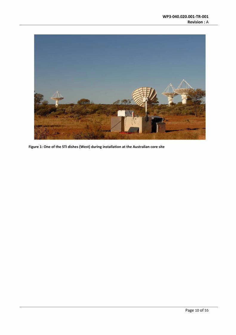
The antennas have been mounted to large, heavy concrete blocks that rest upon the surface, see the

illustration in Figure 1. Underground fibre routing leads to one of the temporary huts that houses

the central electronics in its shielded cabinet, about 200 metres away from the antennas. At the time

of installation and also during the course of the measurements construction activities in the area are

taking place, for building antenna foundations, excavation works, road building and telescope

construction. This has made the environment a very dusty place, which posed challenges to clean

fibre handling.

Antenna #1 West

longitude 116° 37’ 44.4”E 116.629133°

latitude 26° 41’ 48.8”S -26.696883°

altitude 1217 ft 371 m

Antenna #2 East

longitude 116° 37’ 50.5”E 116.630683°

latitude 26° 41’ 52.9”S -26.698017°


Satellite

Optus D3

longitude 156.0°

direction azimuth 61.33°

direction elevation 36.72°

range 38040 km

polarisation tilt 51.6°

frequency band used 11.7-12.2 GHz (central 200 MHz), transmitting and receiving linear

polarisation

Interferometer baseline, derived from coordinate data

Antenna distance 199.1 m

baseline azimuth 129.36°

path difference 60.75 m (relative to West antenna)

Local noon

On 21-06 at 04:15 UTC

Table 1: STI information Australia

WP3-040.020.001-TR-001

Revision : A

of 55

Figure 1: One of the STI dishes (West) during installation at the Australian core site

WP3-040.020.001-TR-001

Revision : A

of 55

5.2 Karoo, South Africa

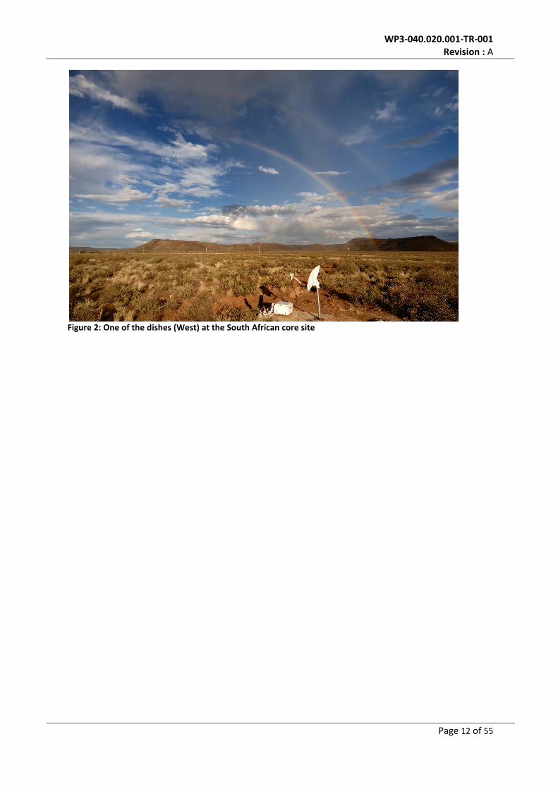
The antennas are mounted to steel posts that are attached to poured concrete foundations, see

Figure 2. The central electronics rack is housed in one of the RFI shielded huts on the site, some tens

of meters away from the nearest antenna. Underground fibres connect the antenna boxes to the

central electronics rack. During the campaign there were no significant construction activities going

on.

Antenna #1 West

longitude 21° 25’ 58.1”E 21.432806°

latitude 30° 45’ 13.8”S 30.753833°


Antenna #2 East

longitude 21° 26’ 04.7”E 21.434639°

latitude 30° 45’ 17.3”S 30.754806°

altitude 3546 ft 1080.8 m

Satellite

Eutelsat W7

longitude 36.0°

direction azimuth 26.96°

direction elevation 50.82°

range 37029 km

frequency band used 12.2-12.7 GHz (central 200 MHz), transmitting linear polarisation, receiving

circular polarisation

Interferometer baseline, derived from coordinate data

Antenna distance 205.9 m

baseline azimuth 121.7°

path difference 11.41 m (relative to East antenna)

Local noon

On 21-06 at 10:36 UTC

Table 2: STI information South Africa

WP3-040.020.001-TR-001

Revision : A

of 55

Figure 2: One of the dishes (West) at the South African core site

WP3-040.020.001-TR-001

Revision : A

of 55

6 Results

6.1 Measurement period

In section 3.2 the period in which measurements were done was discussed in broad terms. Here the

actual periods are specified in which data was acquired that were ultimately used for analysis. This is

done in the form of presenting monthly plots in sections 6.1.1 and 6.1.2. These are standard plots

that come out of the data processing package using all acquired data, regardless of validity due to

system status.

Complete months are shown. For each of the plots a brief explanation of data anomalies is given,

together with the net periods of usable data per month.

Each of the plots in this chapter on the overview of available data, and also in the chapters on data

analysis (6.2), contain four panels, from top to bottom:

1. Raw unwrapped phase: For correct operation sinewave-like variations should be seen as

caused by the diurnal movement of the satellite in its geostationary orbit cube. Because new

files are started at 0 UT the phase is reset to zero at that time, which gives rise to occasional

small steps, or larger steps at that time when during the previous day the unwrapping

algorithm was disturbed or the file wasn’t started at 0 UT for some reason. It is quite easy to

see in this subplot whether valid data is present or not.

2. Correlated amplitude: Nominal levels of ~200 to 700 units in South Africa, and ~200 to 1100

units in Australia indicate correct operation. The variation that is seen is likely due to

transponder channels being switched on and off within the 200 MHz of available bandwidth.

Incorrect operation is indicated by very low amplitude or wildly varying values.

Even though the first two panels are sufficient for judging whether valid data is present, the

following two are included to show the impact on these derived parameters, and also to provide a

complete overview that include small scale anomalies or glitches that need attention for the analysis

in sections 6.2.3 and 6.2.4:

3. Filtered phase: A sinusoid is fitted and removed from the raw phase over the previous 10

minutes. Usually quite clear diurnal tropospheric variation becomes visible.

4. Rms delay: These are corrected zenith delay values, as described in section 4. The diurnal

variations should be obvious.

WP3-040.020.001-TR-001

Revision : A

of 55

6.1.1 Overview of measurements Australia

June 2011: Engineering work on the system up to 10/6. An uninterrupted period starts at 12/8

(T=264), which doesn’t last long when power is lost on 18/6, after which the LO doesn’t regain lock.

No personnel available to attend to the system. Effectively only 12/6 through 17/6 (6 days) are

suitable for analysis.

July 2011: LO lock restored on 4/7. Useful data acquired from 5/7 until 25/7. Then no access, nor

data being acquired for unknown reasons (likely a lengthy power failure). Effectively 20 days of

usable data acquired.

August 2011: System working on 3/8; valid data from 4/8 for the rest of the month (28 days).

Multiple occurrences of drops in correlated amplitude. See data analysis, section 6.2.3.

Figure 3: Overview Australia June 2011

Figure 4: Overview Australia July 2011

Figure 5: Overview Australia August 2011

WP3-040.020.001-TR-001

Revision : A

of 55

September 2011: Usable data from 1/9 through 6/9. Power was interrupted early on 7/9. After

being restored on 9/9 the LO did not lock, which went undetected at that time. When two weeks

later a team worked on the system to replace the LO synthesizer that turned out to be defective the

delay adjustments were finally made, which made a great improvement in the correlated amplitude,

after t≅513 (early on 22/9). Effectively this results in 14 full days of usable data.

Figure 7: Overview Australia October 2011

October 2011: Usable data is acquired from 1/10 through 9/10. On 10/10 the LO has lost lock, which

is reset on the 11th

. On 12/10 through 20/10 data is again acquired, but the quality on 18/10 and

19/10 appears poor (see data analysis section). On 21/10 again the LO has lost lock, until 27/10.

Usable data from 28/10 through 31/10. A total of 22 full days of usable data.

Figure 6: Overview Australia September 2011

WP3-040.020.001-TR-001

Revision : A

of 55

6.1.2 Overview of measurements South Africa

March 2011: Engineering and testing activities until 11-3, followed by a pointing error that was fixed

on 23-3. Usable data from 24/3 onwards, 8 days total.

April 2011: On 28/4 the system stopped writing to disk. That means that usable data was acquired

from 1/4 through 27/4 (27 days).

May 2011: Following a system reboot on 3/5 useful data was acquired until the end of the month (28

full days).

Figure 8: Overview South Africa March 2011

Figure 9: Overview South Africa April 2011

Figure 10: Overview South Africa May 2011

WP3-040.020.001-TR-001

Revision : A

of 55

Figure 11: Overview South Africa June 2011

June 2011: Upgrade activities on 6/6 and 7/6. Another episode of system not writing to disk from

22/6 to 27/6. Useful data acquired on 1/6 through 5/6, 8/6 through 21/6 and 28/6 through 30/6, a

total of 22 days.

Figure 12: Overview South Africa July 2011

July 2011: Complete month of usable data (31 days).

Figure 13: Overview South Africa August 2011

August 2011: System stopped writing to disk, starting early on 16/8. Useful data through 15/8 (15

days).

WP3-040.020.001-TR-001

Revision : A

of 55

WP3-040.020.001-TR-001

Revision : A

of 55

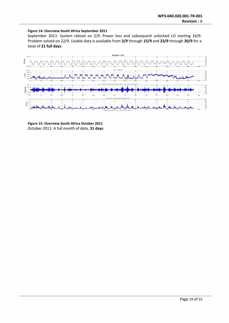
Figure 14: Overview South Africa September 2011

September 2011: System reboot on 2/9. Power loss and subsequent unlocked LO starting 16/9.

Problem solved on 22/9. Usable data is available from 3/9 through 15/9 and 23/9 through 30/9 for a

total of 21 full days.

Figure 15: Overview South Africa October 2011

October 2011: A full month of data, 31 days.

WP3-040.020.001-TR-001

Revision : A

of 55

6.2 Tropospheric delay data

This report contains analysed data in two forms: time series plots of four parameters and cumulative

distribution plots of measured zenith rms delay.

6.2.1 Delay time series

The procedure that was followed was to inspect the availability of usable data, which resulted in the

assessment in the previous sections. Next only full days were processed, resulting in a series of

monthly plots that are presented in the sections that follow.

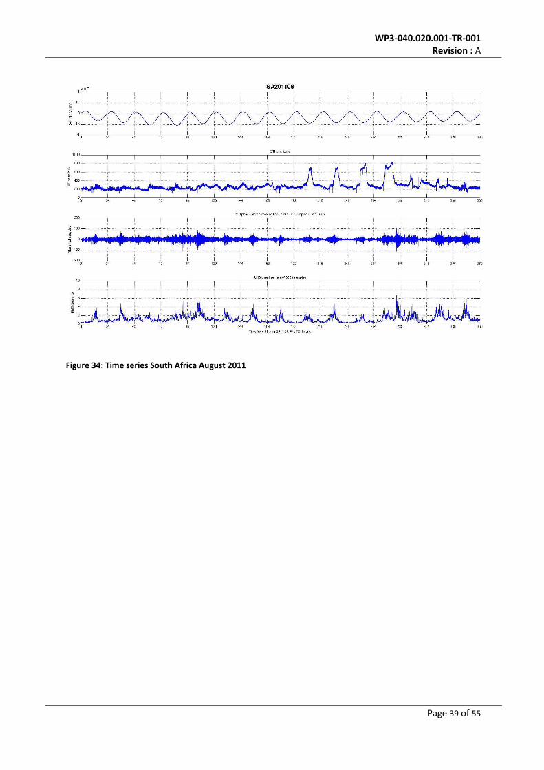
The explanation on what is shown in the panels in each of the plots is repeated here (from section

6.1), from top to bottom:

1. Raw unwrapped phase: For correct operation sinewave-like variations should be seen as

caused by the diurnal movement of the satellite in its geostationary orbit cube. Because new

files are started at 0 UT the phase is reset to zero at that time, which gives rise to occasional

small steps, or larger steps at that time when during the previous day the unwrapping

algorithm was disturbed or the file wasn’t started at 0 UT for some reason.

2. Correlated amplitude: Nominal levels of ~200 to 700 units in South Africa, and ~200 to 1100

units in Australia indicate correct operation. The variation that is seen is likely due to

transponder channels being switched on and off within the 200 MHz of available bandwidth,

see discussion at the end of this paragraph.

3. Filtered phase: A sinusoid is fitted and removed from the raw phase over the previous 10

minutes. Usually quite clear diurnal tropospheric variation becomes visible.

4. Rms delay: These are corrected zenith delay values, as described in section 4. The diurnal

variations should be obvious.

Note that these plots do not have the same time-scale, depending on availability of usable data: they

are shown at their greatest resolution here. This is also true for the vertical scales in the bottom two

panels: the scale used allows best visibility of details.

In these plots it will be apparent that the correlated amplitude traces show variability that one might

not expect. Some of this may be caused by inexact pointing of (one of the dishes), as may be the

case in Australia where a diurnal pattern is seen during much of the time. In South Africa we see

evidence of changes in received signal within the 200 MHz bandwidth. Turning on and off

transponder channels by the satellite operator may be causing the variations. This, however, cannot

be backed up by spectrum analyser evidence. Time constraints have not allowed investigating this

within the reporting period. One might suspect that the changes in signal to noise would have a

noticeable effect on the phase data. This, however, has not been observed in the data. It would

appear that the signal to noise levels have been sufficient for not detecting a clear effect in the

filtered phase data, and that the processing to arrive at the rms delays over 3000 seconds has

removed any remaining effect. This conclusion is supported by the demonstration in the Australian

system where adjusting the cable delays caused a doubling of the correlated amplitude (see 3.2),

without seeing differences in the floor values in the rms delay data, before versus after the change

to the hardware.

6.2.2 Delay cumulative distribution

Further inspection of the time series plots reveals data that was affected by non-tropospherical

causes. It would be incorrect to include that data in the cumulative distribution plots of zenith rms

WP3-040.020.001-TR-001

Revision : A

of 55

delay values. That data is removed before making these distribution plots. Occurrence of this was

indicated in the descriptions of the time series plots.

The plots show three traces:

1. Night-time cumulative distribution (dotted trace): An 8 hour period, centred on local

midnight.

2. Day-time cumulative distribution (dashed trace): An 8 hour period, centred on local noon.

The local noon times that were used are listed in Table 1 for Australia and Table 2 for South

Africa.

3. Overall cumulative distribution (solid trace): All data, regardless of time of day (so including

also dawn and dusk periods).

WP3-040.020.001-TR-001

Revision : A

of 55

6.2.3 Results Australia

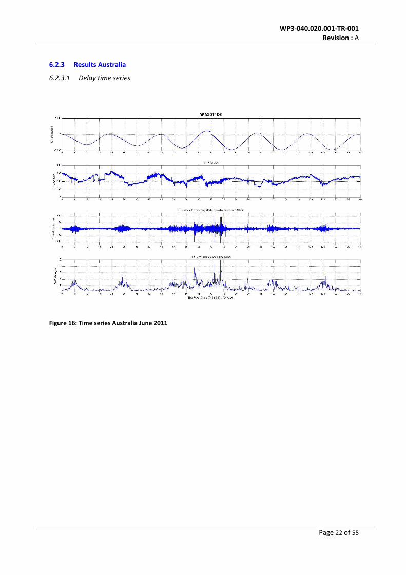
6.2.3.1 Delay time series

Figure 16: Time series Australia June 2011

WP3-040.020.001-TR-001

Revision : A

of 55

The markers indicate glitches that should be disregarded as invalid delay points that have been

removed from data before making the cumulative distribution plots. The brief interruption at t~246

will result only in a ingle zero delay sample in the cumulative distribution and is not removed from

the data.

Figure 17: Time series Australia July 2011

WP3-040.020.001-TR-001

Revision : A

of 55

The markers indicate glitches that should be disregarded as invalid delay points that have been

removed from the data before making the cumulative distribution plots.

Figure 18: Time series Australia August 2011

WP3-040.020.001-TR-001

Revision : A

of 55

Figure 19: Time series Australia September 2011

WP3-040.020.001-TR-001

Revision : A

of 55

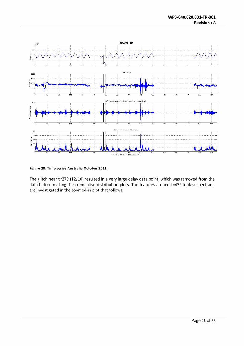
Figure 20: Time series Australia October 2011

The glitch near t~279 (12/10) resulted in a very large delay data point, which was removed from the

data before making the cumulative distribution plots. The features around t=432 look suspect and

are investigated in the zoomed-in plot that follows:

WP3-040.020.001-TR-001

Revision : A

of 55

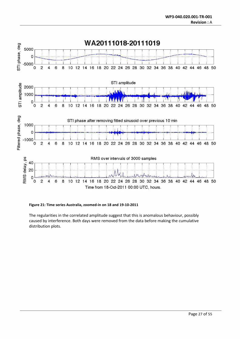
Figure 21: Time series Australia, zoomed-in on 18 and 19-10-2011

The regularities in the correlated amplitude suggest that this is anomalous behaviour, possibly

caused by interference. Both days were removed from the data before making the cumulative

distribution plots.

WP3-040.020.001-TR-001

Revision : A

of 55

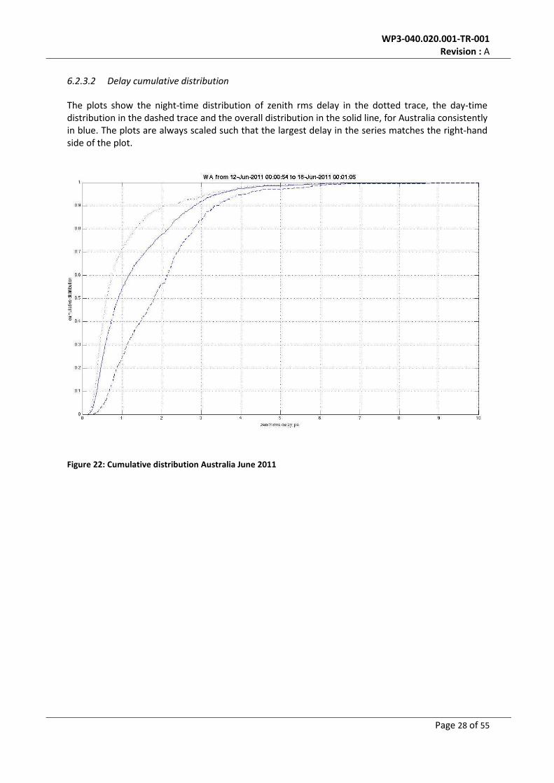
6.2.3.2 Delay cumulative distribution

The plots show the night-time distribution of zenith rms delay in the dotted trace, the day-time

distribution in the dashed trace and the overall distribution in the solid line, for Australia consistently

in blue. The plots are always scaled such that the largest delay in the series matches the right-hand

side of the plot.

Figure 22: Cumulative distribution Australia June 2011

WP3-040.020.001-TR-001

Revision : A

of 55

Figure 24: Cumulative distribution Australia July 2011

Figure 23: Cumulative distribution Australia August 2011

WP3-040.020.001-TR-001

Revision : A

of 55

Figure 26: Cumulative distribution Australia October 2011

Figure 25: Cumulative distribution Australia September 2011

WP3-040.020.001-TR-001

Revision : A

of 55

6.2.4 Results South Africa

6.2.4.1 Delay time series

Note that occurrences of low amplitude were seen around t~160, with no obvious effects on the rms

delay. This data was not removed before making the cumulative distribution plots.

Figure 27: Time series South Africa March 2011

WP3-040.020.001-TR-001

Revision : A

of 55

The marker indicates a glitch that should be disregarded as an invalid delay point that has been

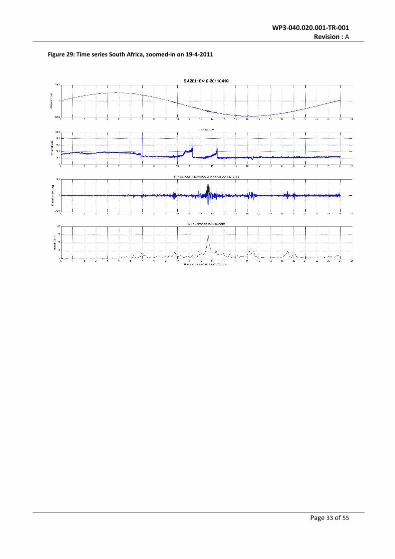
removed from the data before making the cumulative distribution plots. The delay feature on 19/4

(starting t=432) appears to be a real tropospheric event and is not removed from the data, but will

give a 31ps outlier in the cumulative distribution plot for this month. A zoomed in plot for this day

follows:

Figure 28: Time series South Africa April 2011

WP3-040.020.001-TR-001

Revision : A

of 55

Figure 29: Time series South Africa, zoomed-in on 19-4-2011

WP3-040.020.001-TR-001

Revision : A

of 55

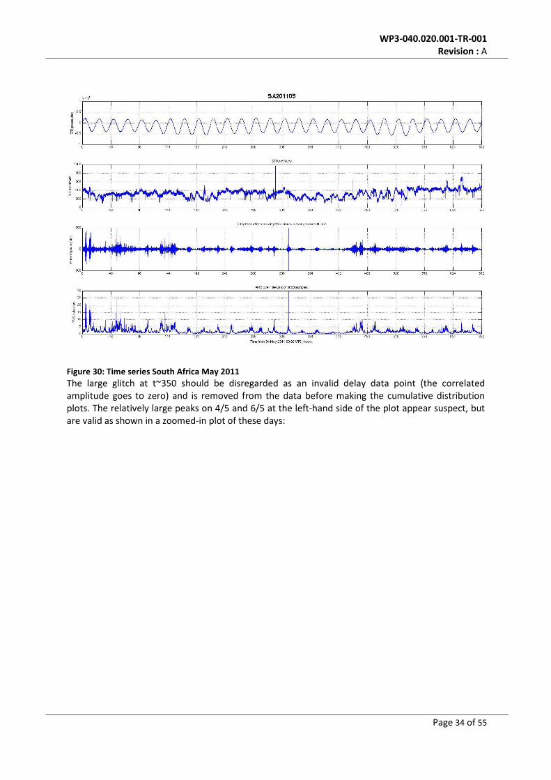
The large glitch at t~350 should be disregarded as an invalid delay data point (the correlated

amplitude goes to zero) and is removed from the data before making the cumulative distribution

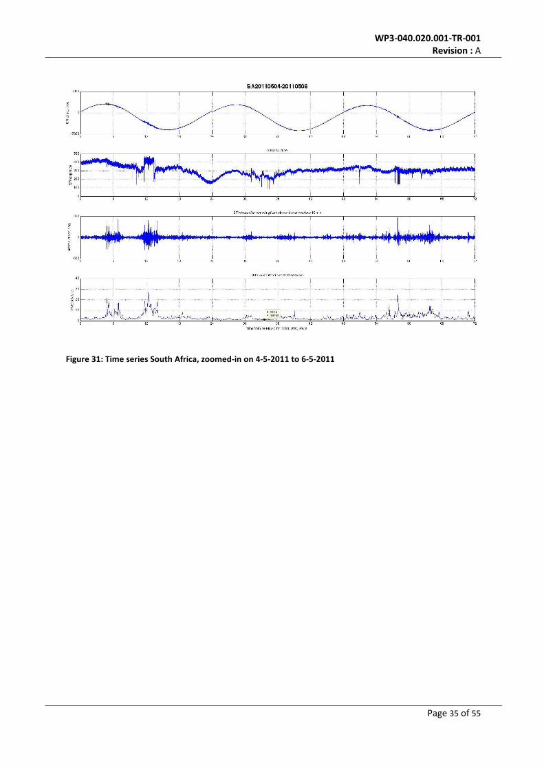
plots. The relatively large peaks on 4/5 and 6/5 at the left-hand side of the plot appear suspect, but

are valid as shown in a zoomed-in plot of these days:

Figure 30: Time series South Africa May 2011

WP3-040.020.001-TR-001

Revision : A

of 55

Figure 31: Time series South Africa, zoomed-in on 4-5-2011 to 6-5-2011

WP3-040.020.001-TR-001

Revision : A

of 55

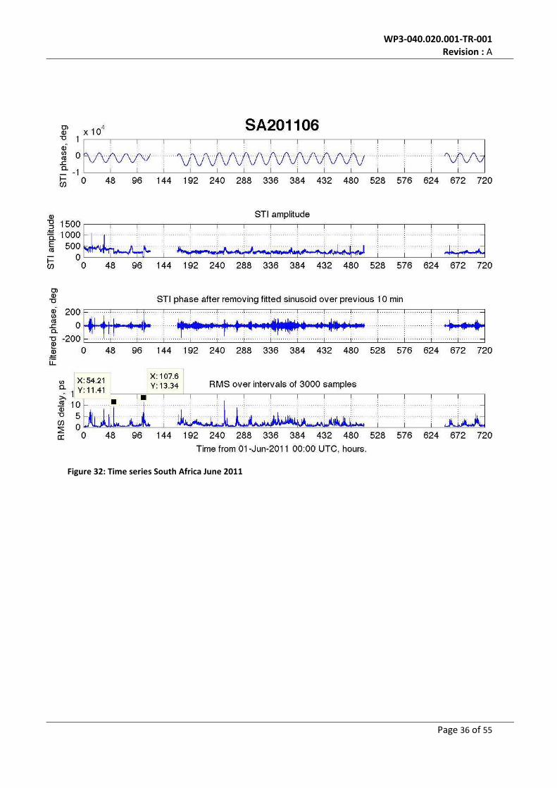
Figure 32: Time series South Africa June 2011

WP3-040.020.001-TR-001

Revision : A

of 55

The markers indicate glitches caused by sudden drops in correlated amplitude that should be

disregarded as invalid data and that have been removed from the data before making the

cumulative distribution plots.

WP3-040.020.001-TR-001

Revision : A

of 55

Figure 33: Time series South Africa July 2011

WP3-040.020.001-TR-001

Revision : A

of 55

Figure 34: Time series South Africa August 2011

WP3-040.020.001-TR-001

Revision : A

of 55

The event at t=109 (7/9) cannot be qualified as a tropospheric effect as becomes clear in the

zoomed-in view for that day in the following plot. It appears that work was being done on the

satellite transponder(s), causing rapid fluctuations in amplitude with an impact on delay data. This

day was removed from the data before making the cumulative distribution plots.

Figure 35: Time series South Africa September 2011

WP3-040.020.001-TR-001

Revision : A

of 55

Figure 36: Time series South Africa, zoomed-in on 7-09-2011

This plot demonstrates that the delay data around t=13 cannot be attributed to the troposphere. In

this plot note the marker that indicates very low rms delay values.

WP3-040.020.001-TR-001

Revision : A

of 55

Figure 37: Time series South Africa October 2011

WP3-040.020.001-TR-001

Revision : A

of 55

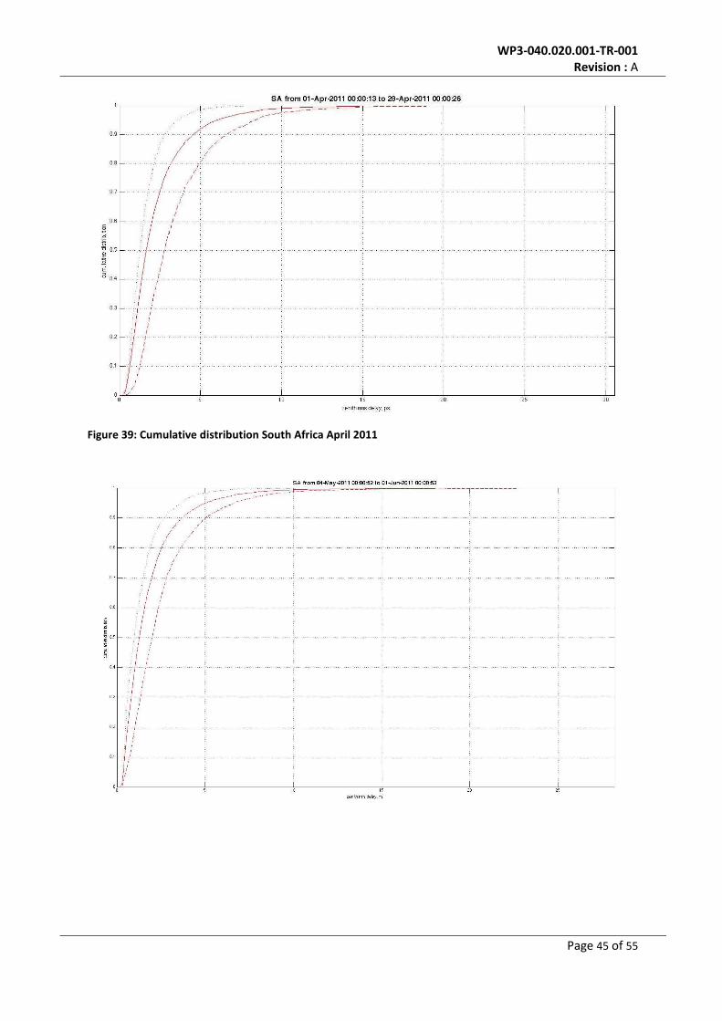
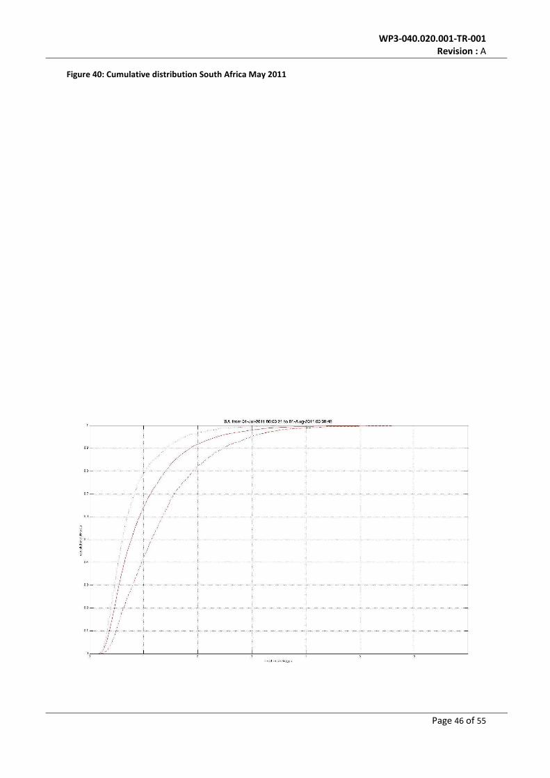
6.2.4.2 Delay cumulative distribution

The plots show the night-time distribution of zenith rms delay in the dotted trace, the day-time

distribution in the dashed trace and the overall distribution in the solid line, for South Africa

consistently in red. The plots are always scaled such that the largest delay in the series matches the

right-hand side of the plot.

Figure 38: Cumulative distribution South Africa March 2011

WP3-040.020.001-TR-001

Revision : A

of 55

WP3-040.020.001-TR-001

Revision : A

of 55

Figure 39: Cumulative distribution South Africa April 2011

WP3-040.020.001-TR-001

Revision : A

of 55

Figure 40: Cumulative distribution South Africa May 2011

WP3-040.020.001-TR-001

Revision : A

of 55

Figure 42: Cumulative distribution South Africa July 2011

Figure 43: Cumulative distribution South Africa August 2011

Figure 41: Cumulative distribution South Africa June 2011

WP3-040.020.001-TR-001

Revision : A

of 55

Figure 44: Cumulative distribution South Africa September 2011

WP3-040.020.001-TR-001

Revision : A

of 55

Figure 45: Cumulative distribution South Africa October 2011

6.2.5 Comparisons between sites

The cumulative distributions are used to extract numeric data that can be used to compare the

measurements at the two sites. In

monthly overall, daytime and night

95 percentile rms delays are listed. Also the number of samples on which these statistics are based

are listed. Even though the numbers

only be made by comparing same months for the two countries, which is rather limited for the

reasons explained earlier. The South African data, extending over more months than the Australian

set, suggest a seasonal effect on the delays values. This is also illustrated in a plot of median delay

values over the sampled months,

the top trace represents daytime statistics, the middle trace overall and the bottom trace night

statistics.

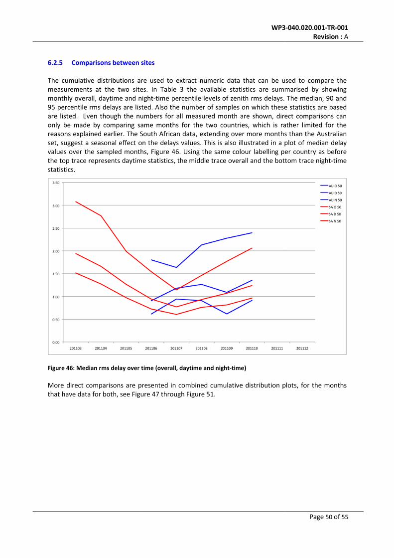
Figure 46: Median rms delay over time (overall, daytime and night

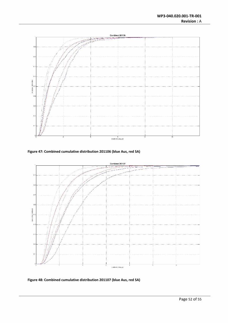
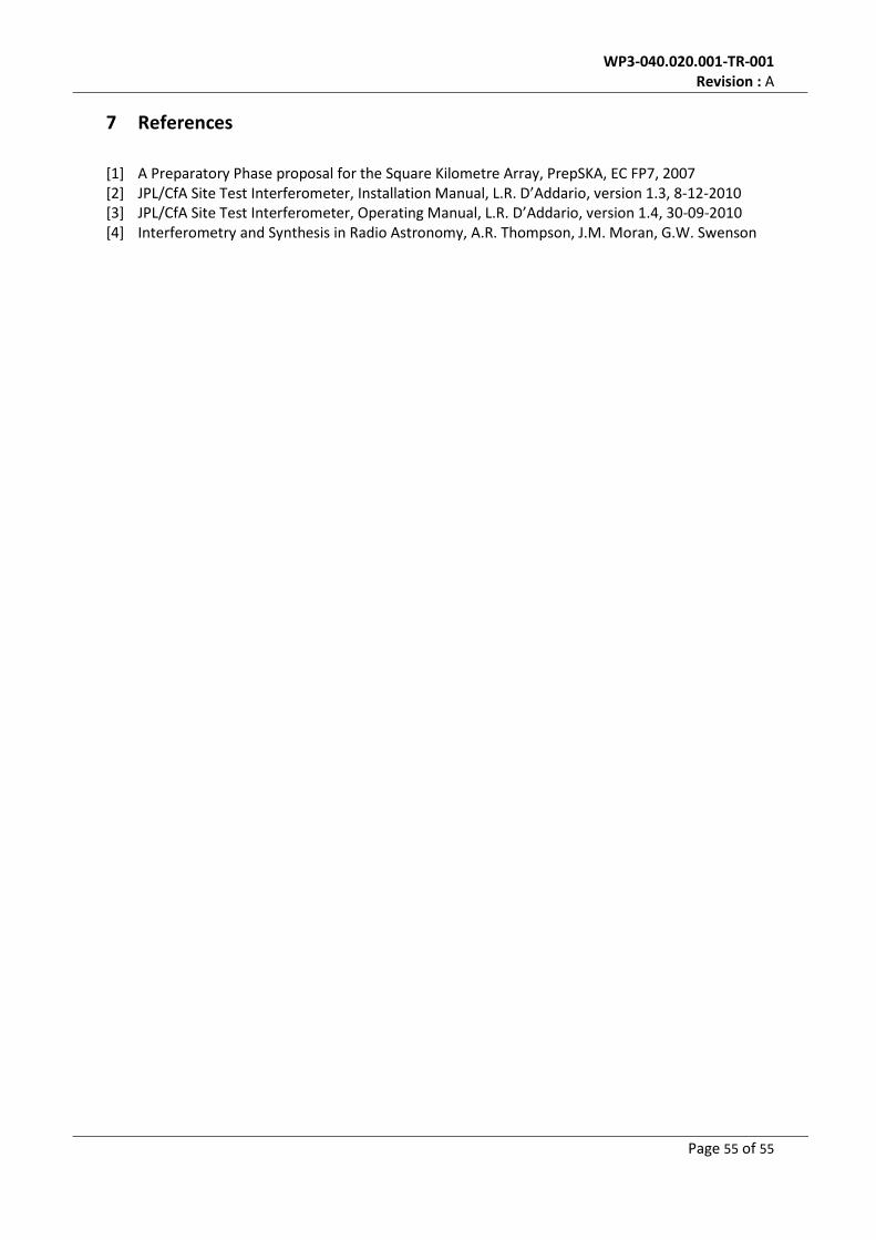
More direct comparisons are presented in combined cumulative distribution plots, for the months

that have data for both, see Figure

WP3

Comparisons between sites


measurements at the two sites. In Table 3 the available statistics are summarised by showing

monthly overall, daytime and night-time percentile levels of zenith rms delays. The median, 90 and


are listed. Even though the numbers for all measured month are shown, direct comparisons can



gest a seasonal effect on the delays values. This is also illustrated in a plot of median delay

values over the sampled months, Figure 46. Using the same colour labelling per country as before

the top trace represents daytime statistics, the middle trace overall and the bottom trace night

: Median rms delay over time (overall, daytime and night-time)

arisons are presented in combined cumulative distribution plots, for the months

Figure 47 through Figure 51.

WP3-040.020.001-TR-001

Revision : A

of 55


mmarised by showing

time percentile levels of zenith rms delays. The median, 90 and


for all measured month are shown, direct comparisons can



gest a seasonal effect on the delays values. This is also illustrated in a plot of median delay

ing per country as before

the top trace represents daytime statistics, the middle trace overall and the bottom trace night-time

arisons are presented in combined cumulative distribution plots, for the months

WP3-040.020.001-TR-001

Revision : A

of 55

Table 3: Cumulative Distribution Statistics over time

WP3-040.020.001-TR-001

Revision : A

of 55

Figure 47: Combined cumulative distribution 201106 (blue Aus, red SA)


WP3-040.020.001-TR-001

Revision : A

of 55



WP3-040.020.001-TR-001

Revision : A

of 55

7 References

[1] A Preparatory Phase proposal for the Square Kilometre Array, PrepSKA, EC FP7, 2007

[2] JPL/CfA Site Test Interferometer, Installation Manual, L.R. D’Addario, version 1.3, 8-12-2010

[3] JPL/CfA Site Test Interferometer, Operating Manual, L.R. D’Addario, version 1.4, 30-09-2010

[4] Interferometry and Synthesis in Radio Astronomy, A.R. Thompson, J.M. Moran, G.W. Swenson

Tropospheric stability at candidate SKA sites 1 · PDF fileWordprocessor MsWord Word 2007...

Documents

Transcript of Tropospheric stability at candidate SKA sites 1 · PDF fileWordprocessor MsWord Word 2007...