Trip Distribution Lecture 9 Norman W. Garrick

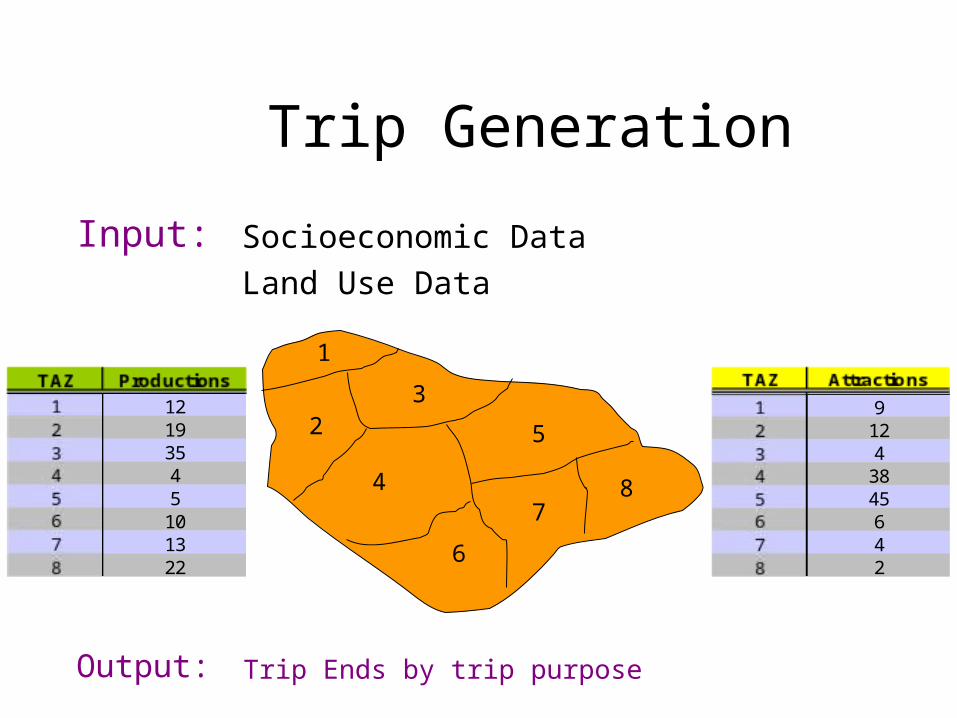
Trip Generation

1

23

4

5

6

87

TAZ Productions

1 122 193 354 45 56 107 138 22

TAZ Attractions

1 92 123 44 385 456 67 48 2

Input:

Output:

Socioeconomic Data

Land Use Data

Trip Ends by trip purpose

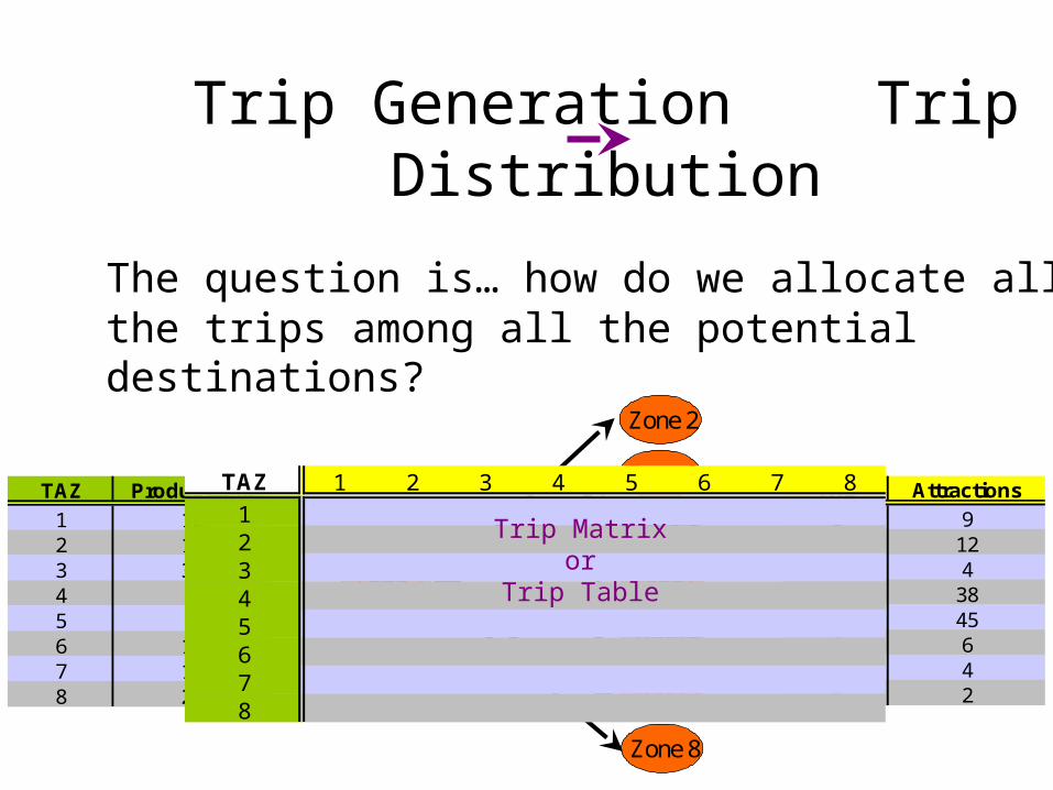
Trip Generation Trip Distribution

The question is… how do we allocate all the trips among all the potential destinations?

TAZ Productions

1 122 193 354 45 56 107 138 22

TAZ Attractions

1 92 123 44 385 456 67 48 2

Zone 2

Zone 3

Zone 4

Zone 5

Zone 6

Zone 7

Zone 8

Zone 1

TAZ 1 2 3 4 5 6 7 8

12345678

Trip Matrixor

Trip Table

Trip Distribution

Trip Distribution

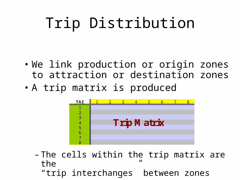
• We link production or origin zones to attraction or destination zones

• A trip matrix is produced

– The cells within the trip matrix are the “trip interchanges” between zones

Zone 1

TAZ 1 2 3 4 5 6 7 8

12345678

Trip Matrix

Basic Assumptions of Trip Distribution

• Number of trips decrease with COST between zones

• Number of trips increase with zone “attractiveness”

Methods of Trip Distribution

I. Growth Factor Models

II. Gravity Model

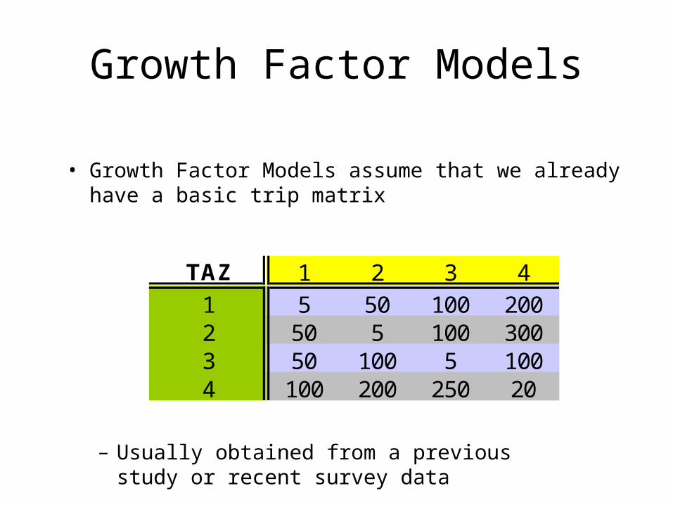
Growth Factor Models

• Growth Factor Models assume that we already have a basic trip matrix

– Usually obtained from a previous study or recent survey data

TAZ 1 2 3 4

1 5 50 100 2002 50 5 100 3003 50 100 5 1004 100 200 250 20

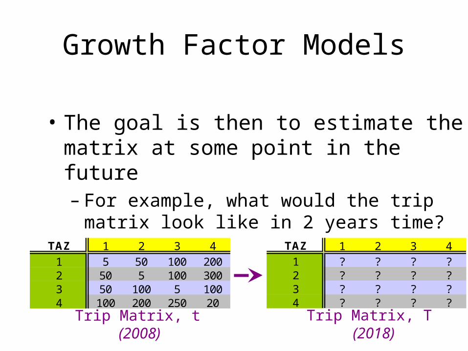
Growth Factor Models

• The goal is then to estimate the matrix at some point in the future – For example, what would the trip matrix look like

in 2 years time?

TAZ 1 2 3 4

1 5 50 100 2002 50 5 100 3003 50 100 5 1004 100 200 250 20

Trip Matrix, t (2008)

Trip Matrix, T (2018)

TAZ 1 2 3 4

1 ? ? ? ?2 ? ? ? ?3 ? ? ? ?4 ? ? ? ?

Some of the More Popular Growth Factor Models

• Uniform Growth Factor

• Singly-Constrained Growth Factor

• Average Factor

• Detroit Factor

• Fratar Method

Uniform Growth Factor Model

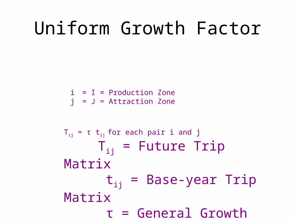
Uniform Growth Factor

Tij = τ tij for each pair i and j

Tij = Future Trip Matrix tij = Base-year Trip Matrix τ = General Growth Rate

i = I = Production Zone j = J = Attraction Zone


TAZ 1 2 3 4

1 5 50 100 2002 50 5 100 3003 50 100 5 1004 100 200 250 20

TAZ 1 2 3 4

1 6 60 120 2402 60 6 120 3603 60 120 6 1204 120 240 300 24

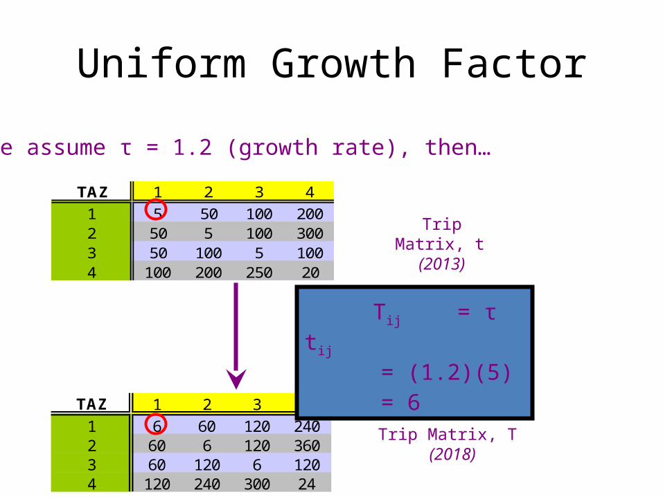
Trip Matrix, t (2013)

Trip Matrix, T (2018)

If we assume τ = 1.2 (growth rate), then…

Tij = τ tij

= (1.2)(5)= 6


The Uniform Growth Factor is typically used for over a 1 or 2 year horizon

However, assuming that trips growat a standard uniform rate is a fundamentally flawed

concept

The Gravity Model

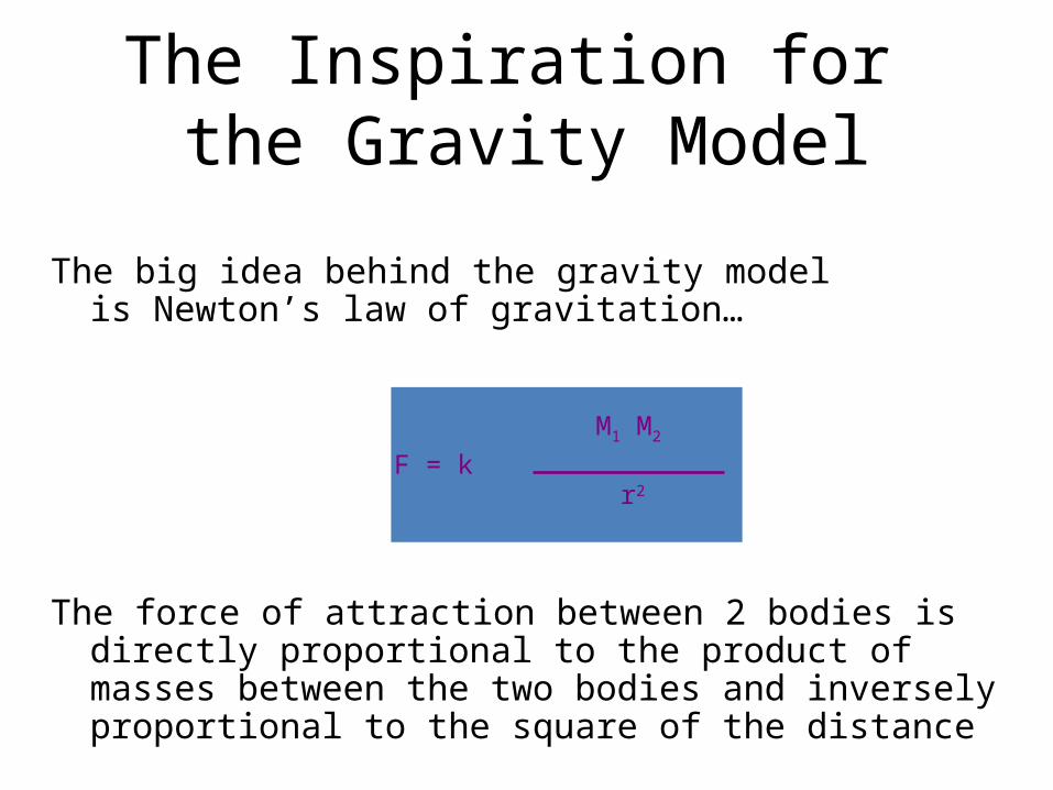
The big idea behind the gravity model is Newton’s law of gravitation…

The force of attraction between 2 bodies is directly proportional to the product of masses between the two bodies and inversely proportional to the square of the distance

The Inspiration for the Gravity Model

F = k

M1 M2

r2

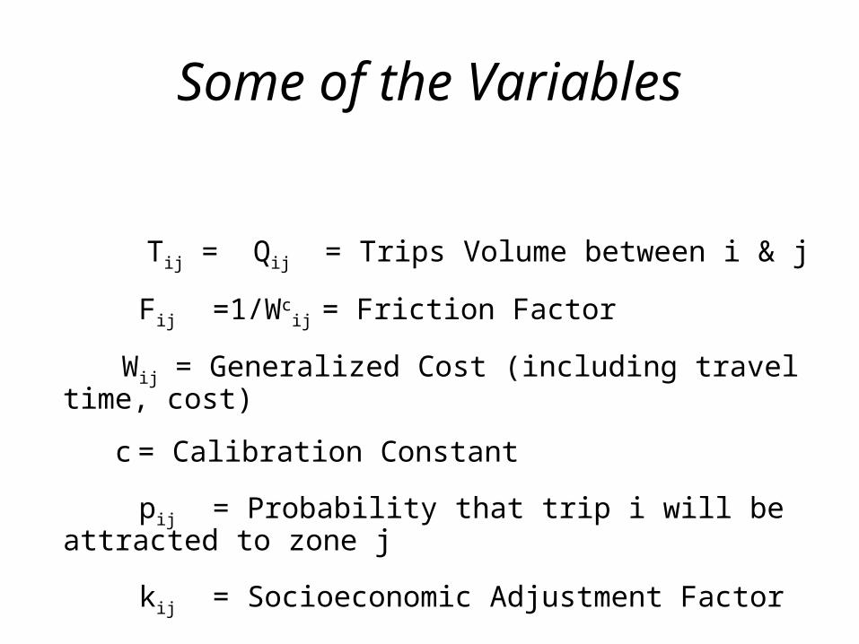
Some of the Variables

Tij = Qij = Trips Volume between i & j

Fij =1/Wcij = Friction Factor

Wij = Generalized Cost (including travel time, cost)

c= Calibration Constant

pij = Probability that trip i will be attracted to zone j

kij = Socioeconomic Adjustment Factor

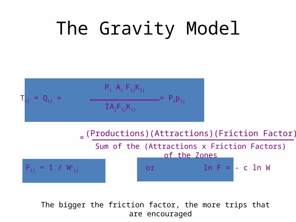
The Gravity Model

The bigger the friction factor, the more trips that are encouraged

Tij = Qij =

Pi Aj FijKij

ΣAjFijKij

Fij = 1 / Wcij

(Productions)(Attractions)(Friction Factor)

Sum of the (Attractions x Friction Factors) of the Zones=

= Pipij

or ln F = - c ln W

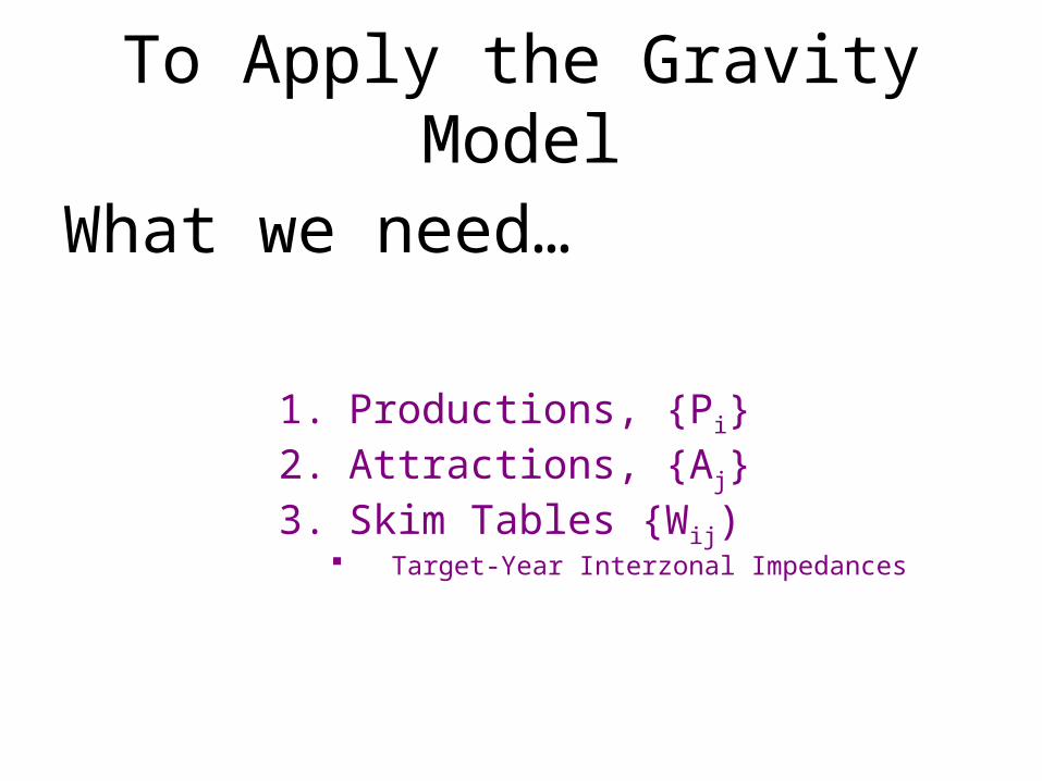
To Apply the Gravity Model

What we need…

1. Productions, {Pi}2. Attractions, {Aj}3. Skim Tables {Wij)

Target-Year Interzonal Impedances

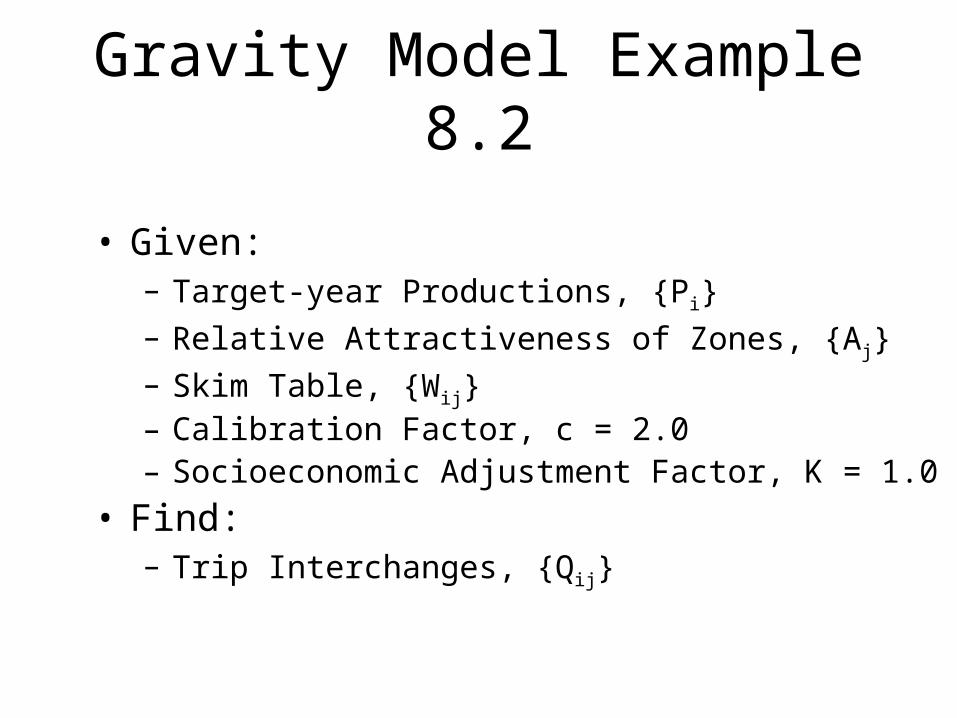
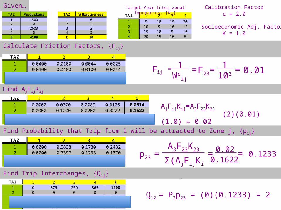
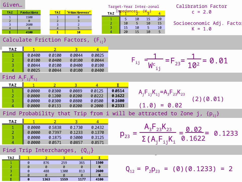
Gravity Model Example 8.2

• Given:– Target-year Productions, {Pi}

– Relative Attractiveness of Zones, {Aj}

– Skim Table, {Wij}– Calibration Factor, c = 2.0– Socioeconomic Adjustment Factor, K = 1.0

• Find:– Trip Interchanges, {Qij}

Σ(AjFijKij)

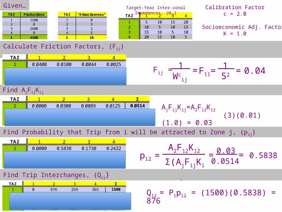
Calculate Friction Factors, {Fij}

TAZ Productions

1 15002 03 26004 0Σ 4100

TAZ "Attractiveness"

1 02 33 24 5Σ 10

TAZ 1 2 3 4

1 5 10 15 202 10 5 10 153 15 10 5 104 20 15 10 5

Calibration Factorc = 2.0

Socioeconomic Adj. FactorK = 1.0

TAZ 1 2 3 4

1 0.0400 0.0100 0.0044 0.00252 0.0100 0.0400 0.0100 0.00443 0.0044 0.0100 0.0400 0.01004 0.0025 0.0044 0.0100 0.0400

TAZ 1 2 3 4 Σ

1 0.0000 0.0300 0.0089 0.0125 0.05142 0.0000 0.1200 0.0200 0.0222 0.16223 0.0000 0.0300 0.0800 0.0500 0.16004 0.0000 0.0133 0.0200 0.2000 0.2333

TAZ 1 2 3 4

1 0.0000 0.5838 0.1730 0.24322 0.0000 0.7397 0.1233 0.13703 0.0000 0.1875 0.5000 0.31254 0.0000 0.0571 0.0857 0.8571

TAZ 1 2 3 4 Σ

1 0 876 259 365 15002 0 0 0 0 03 0 488 1300 813 26004 0 0 0 0 0Σ 0 1363 1559 1177 4100

Target-Year Inter-zonal Impedances, {W ij}

F11=152 = 0.04

AjFijKij=A2F12K12

(3)(0.01)(1.0) = 0.03

Given…

Find AjFijKij

Find Probability that Trip from i will be attracted to Zone j, {p ij}

Find Trip Interchanges, {Qij}

p12 =A2F12K12

0.0514= 0.03 = 0.5838

Q12 = P1p12 = (1500)(0.5838) = 876

Fij =1

Wcij

=

Σ(AjFijKij)

Calculate Friction Factors, {Fij}

TAZ Productions

1 15002 03 26004 0Σ 4100

TAZ "Attractiveness"

1 02 33 24 5Σ 10

TAZ 1 2 3 4

1 5 10 15 202 10 5 10 153 15 10 5 104 20 15 10 5

Calibration Factorc = 2.0

Socioeconomic Adj. FactorK = 1.0

TAZ 1 2 3 4

1 0.0400 0.0100 0.0044 0.00252 0.0100 0.0400 0.0100 0.00443 0.0044 0.0100 0.0400 0.01004 0.0025 0.0044 0.0100 0.0400

TAZ 1 2 3 4 Σ

1 0.0000 0.0300 0.0089 0.0125 0.05142 0.0000 0.1200 0.0200 0.0222 0.16223 0.0000 0.0300 0.0800 0.0500 0.16004 0.0000 0.0133 0.0200 0.2000 0.2333

TAZ 1 2 3 4

1 0.0000 0.5838 0.1730 0.24322 0.0000 0.7397 0.1233 0.13703 0.0000 0.1875 0.5000 0.31254 0.0000 0.0571 0.0857 0.8571

TAZ 1 2 3 4 Σ

1 0 876 259 365 15002 0 0 0 0 03 0 488 1300 813 26004 0 0 0 0 0Σ 0 1363 1559 1177 4100

Target-Year Inter-zonal Impedances, {W ij}

F23=1

102 = 0.01

AjFijKij=A3F23K23

(2)(0.01)(1.0) = 0.02

Given…

Find AjFijKij

Find Probability that Trip from i will be attracted to Zone j, {p ij}

Find Trip Interchanges, {Qij}

p23 =A3F23K23

0.1622= 0.02 = 0.1233

Q12 = P2p23 = (0)(0.1233) = 2

Fij =1

Wcij

=

Keep in mind that the socioeconomic factor, K, can be a matrix of values rather than just

one value

TAZ 1 2 3 4

1 1.4 1.2 1.7 1.92 1.2 1.1 1.1 1.43 1.7 1.1 1.5 1.34 1.9 1.4 1.3 1.6

The Problem with K-Factors

• Although K-Factors may improve the model in the base year, they assume that these special conditions will carry over to future years and scenarios– This limits model sensitivity and undermines the

model’s ability to predict future travel behavior

• The need for K-factors often is a symptom of other model problems. – Additionally, the use of K-factors makes it more

difficult to figure out the real problems

Limitations of the Gravity Model

• Too much of a reliance on K-Factors in calibration • External trips and intrazonal trips cause difficulties• The skim table impedance factors are often too

simplistic to be realistic– Typically based solely upon vehicle travel times

• At most, this might include tolls and parking costs– Almost always fails to take into account how things such

as good transit and walkable neighborhoods affect trip distribution

– No obvious connection to behavioral decision-making

Trip Distribution Lecture 9 Norman W. Garrick

Documents

Transcript of Trip Distribution Lecture 9 Norman W. Garrick