Trienko Lups Grobler - repository.up.ac.za
223
SEQUENTIAL AND NON-SEQUENTIAL HYPERTEMPORAL CLASSIFICATION AND CHANGE DETECTION OF MODIS TIME-SERIES by Trienko Lups Grobler Submitted in partial fulfilment of the requirements for the degree Philosophiae Doctor (Engineering) in the Department of Electrical, Electronic and Computer Engineering Faculty of Engineering, Built Environment and Information Technology UNIVERSITY OF PRETORIA September 2012 © University of Pretoria
Transcript of Trienko Lups Grobler - repository.up.ac.za

SEQUENTIAL AND NON-SEQUENTIAL HYPERTEMPORAL CLASSIFICATION AND
CHANGE DETECTION OF MODIS TIME-SERIES
by
Trienko Lups Grobler
Submitted in partial fulfilment of the requirements for the degree
Philosophiae Doctor (Engineering)
in the
Department of Electrical, Electronic and Computer Engineering
Faculty of Engineering, Built Environment and Information Technology
UNIVERSITY OF PRETORIA
September 2012
©© UUnniivveerrssiittyy ooff PPrreettoorriiaa

SUMMARY
SEQUENTIAL AND NON-SEQUENTIAL HYPERTEMPORAL CLASSIFICATION AND
CHANGE DETECTION OF MODIS TIME-SERIES
by
Trienko Lups Grobler
Promoter(s): Prof. J.C. Olivier, Dr. W. Kleynhans and Dr. A.J. van Zyl
Department: Electrical, Electronic and Computer Engineering
University: University of Pretoria
Degree: Philosophiae Doctor (Engineering)
Keywords: noise-harmonic features, Coloured Simple Harmonic Oscillator, Sup-
port Vector Machine, Moderate Resolution Imaging Spectroradiometer,
Cumulative Sum, Ornstein-Uhlenbeck process, inductive simulator, hy-
pertemporal classification, hypertemporal change detection, sequential
analysis
Satellites provide humanity with data to infer properties of the earth that were impossible a century
ago. Humanity can now easily monitor the amount of ice found on the polar caps, the size of forests
and deserts, the earth’s atmosphere, the seasonal variation on land and in the oceans and the surface
temperature of the earth. In this thesis, new hypertemporal techniques are proposed for the settlement
detection problem in South Africa. The hypertemporal techniques are applied to study areas in the
Gauteng and Limpopo provinces of South Africa. To be more specific, new sequential (windowless)
and non-sequential hypertemporal techniques are implemented. The time-series employed by the new
hypertemporal techniques are obtained from the Moderate Resolution Imaging Spectroradiometer
(MODIS) sensor, which is on board the earth observations satellites Aqua and Terra. One MODIS
dataset is constructed for each province.
A Support Vector Machine (SVM) [1] that uses a novel noise-harmonic feature set is implemented to
detect existing human settlements. The noise-harmonic feature set is a non-sequential hypertemporal
feature set and is constructed by using the Coloured Simple Harmonic Oscillator (CSHO) [2]. The
CSHO consists of a Simple Harmonic Oscillator (SHO) [3], which is superimposed on the Ornstein-

Uhlenbeck process [4]. The noise-harmonic feature set is an extension of the classic harmonic feature
set [5]. The classic harmonic feature set consists of a mean and a seasonal component. For the case
studies in this thesis, it is observed that the noise-harmonic feature set not only extends the harmonic
feature set, but also improves on its classification capability.
The Cumulative Sum (CUSUM) algorithm was developed by Page in 1954 [6]. In its original form
it is a sequential (windowless) hypertemporal change detection technique. Windowed versions of
the algorithm have been applied in a remote sensing context. In this thesis CUSUM is used in its
original form to detect settlement expansion in South Africa and is benchmarked against the classic
band differencing change detection approach of Lunetta et al., which was developed in 2006 [7].
In the case of the Gauteng study area, the CUSUM algorithm outperformed the band differencing
technique. The exact opposite behaviour was seen in the case of the Limpopo dataset.
Sequential hypertemporal techniques are data-intensive and an inductive MODIS simulator was the-
refore also developed (to augment datasets). The proposed simulator is also based on the CSHO.
Two case studies showed that the proposed inductive simulator accurately replicates the temporal
dynamics and spectral dependencies found in MODIS data.

OPSOMMING
SEKWENSIËLE EN NIE-SEKWENSIËLE HIPERTEMPORALE KLASSIFIKASIE EN
VERANDERING-OPSPORING VAN MABS-TYDSREEKSE
deur
Trienko Lups Grobler
Promotor(s): Prof. J.C. Olivier, Dr. W. Kleynhans en Dr. A.J. van Zyl
Departement: Elektriese, Elektroniese en Rekenaar-Ingenieurswese
Universiteit: Universiteit van Pretoria
Graad: Philosophiae Doctor (Ingenieurswese)
Sleutelwoorde: harmoniesegeraas-kenmerkstel, Gekleurde Eenvoudige Harmoniese
Ossillator, Steunvektormasjien, Matigeresolusie- Beeldskeppende
Spektrale Radio-ontvanger, Kumulatiewesom, Ornstein-Uhlenbeck
proses, induktiewe simulator, hipertemporale klassifikasie, hipertempo-
rale verandering-opsporing, sekwensiële analiese
Satelliete gee die mensdom die geleentheid om dinge van die aarde te leer wat nie ’n eeu gelede
moontlik was nie. Die mensdom kan nou maklik die hoeveelheid ys op die pole, die grootte van
woude en woestyne, die aarde se atmosfeer, die seisoenale veranderinge op land en in die oseane,
asook die temperatuur op die aarde se oppervlak monitor. In hierdie proefskrif word nuwe hipertem-
porale tegnieke vir die sogenaamde nedersettingsopsporingsprobleem in Suid-Afrika beskryf. Die
nuwe hipertemporale tegnieke word toegepas op studie-areas in die Gauteng- en Limpopoprovinsies
van Suid-Afrika. Om meer spesifiek te wees, nuwe sekwensiële (vensterlose) en nie-sekwensiële
hipertemporale tegnieke word bespreek. Die tydsreekse wat deur die hipertemporale tegnieke be-
nodig word, word deur die Matigeresolusie- Beeldskeppende Spektrale Radio-ontvanger (MABS)
sensor verskaf, wat gemonteer is op die aardobservasiesatelliete Aqua en Terra. Een MABS-datastel
is saamgestel vir elke provinsie.
’n Steunvektormasjien (SVM) [1] wat ’n nuwe harmoniesegeraas-kenmerkstel gebruik om bes-
taande nedersettings op te spoor, is geïmplementeer. Die nuwe harmoniesegeraas-kenmerkstel
is ’n nie-sekwensiële hipertemporale-kenmerkstel en is saamgestel deur die Gekleurde Eenvou-

dige Harmoniese Ossillator (GEHO) te gebruik [2]. Die GEHO bestaan uit ’n Eenvoudige Har-
moniese Ossillator (EHO) [3] wat gesuperponeer is op die Ornstein-Uhlenbeck-proses [4]. Die
harmoniesegeraas-kenmerkstel is ’n uitbreiding van die klassieke harmoniese-kenmerkstel [5]. Die
klassieke harmoniese-kenmerkstel bestaan uit ’n gemiddelde en ’n seisoenale komponent. Aan
die hand van die gevallestudies in hierdie proefskrif is daar gevind dat die harmoniesegeraas-
kenmerkstel nie net ’n uitbreiding van die klassieke harmoniese-kenmerkstel is nie, maar dat
die harmoniesegeraas-kenmerkstel ook die klassifikasie-vermoë van die klassieke harmoniese-
kenmerkstel verbeter.
Die Kumulatiewesom- (KUMSOM) algoritme is in 1954 deur Page ontwikkel [6]. In sy oorspronklike
vorm is dit ’n sekwensiële hipertemporale veranderingopsporingstegniek. Afgeknotte weergawes van
die algoritme is al vantevore in ’n afstandswaarneming-konteks gebruik. In hierdie proefskrif word
KUMSOM in sy oorspronklike vensterlose vorm gebruik om die vorming van nuwe nedersettings
in Suid-Afrika op te spoor. Die KUMSOM-algoritme word ook met die bandaftrekkingmetode ver-
gelyk, wat in 2006 deur Lunetta et al. ontwikkel is [7]. In die geval van die Gauteng-gevallestudie
lewer KUMSOM beter resultate as die bandaftrekkingmetode. Die presiese teenoorgestelde gedrag is
waargeneem in die geval van Limpopo.
Sekwensiële hipertemporale tegnieke is baie data-intensief, gevolglik is ’n induktiewe MABS-
simulator ontwerp wat datastelle kan vergroot. Die nuwe simulator is ook gebaseer op die GEHO.
Twee gevallestudies het gewys dat die induktiewe simulator wel die temporale dinamika en spektrale
afhanklikheid kan dupliseer wat voorkom in MABS-data.

ACKNOWLEDGEMENTS
In the first place I would like to thank God for the many blessings that I have received out of his
gracious hand. Second, I would like to thank my supervisors, Prof. J.C. Olivier, Dr. W. Kleynhans
and Dr. A.J. van Zyl, and my colleagues, Dr. B.P. Salmon and Mr. E.R. Ackermann, for their technical
contributions. I would also like to thank my wife, Mrs. C.I. Grobler, friends and family (especially my
parents and brother Mr. P.N. Grobler) for their support. Lastly, I would like to thank my sister, Mrs.
J.B. Louw, who helped me obtain some of the reference material used in this thesis. The Council for
Scientific and Industrial Research (CSIR) (especially Mr. A. van der Merwe) should also be thanked
for their financial contribution. The thesis was proofread by Mrs. M.B. Bradley.
In die begin het God die hemel en die aarde geskep. Die aarde was heeltemal onbewoonbaar, dit was
donker op die diep waters, maar die Gees van God het oor die waters gesweef. Toe het God gesê:
“Laat daar lig wees!” En daar was lig.
Genesis 1:1-3, Bybel Nuwe Vertaling, 1983
This dissertation is dedicated to my wife and parents.

LIST OF ABBREVIATIONS
AG Asymmetric Gaussian
AIRS Atmospheric Infrared Sounder
AMSR-E Advanced Microwave Scanning Radiometer-EOS
AMSU Advanced Microwave Sounding Unit
ANN Artificial Neural Network
AR Autoregressive
ARL Average Run Length
ASN Average Sample Number
ASTER Advanced Spaceborne Thermal Emission and Reflection Radiometer
ATMS Advanced Technology Microwave Sounder
AVHRR Advanced Very High Resolution Radiometer
B Blue
BB Blackbody
BFAST Breaks for Additive Seasonal and Trend
BOB Bureau of Budget
BRDF Bidirectional Reflectance Distribution Function
CERES Clouds and the Earth’s Radiant Energy System
CSIR Council for Scientific and Industrial Research

CrIS Cross-track Infrared Sounder
CSHO Coloured Simple Harmonic Oscillator
CUSUM Cumulative Sum
CVA Change Vector Analysis
CZCS Coastal Zone Color Scanner
DAAC Distributed Active Archive Center
DL Double Logistic
DN Digital Number
DOD Department of Defense
DOI Department of the Interior
EDOS EOS Data and Operations System
EHO Eenvoudige Harmoniese Ossillator
EOS Earth Observing System
EOSMRWG EOS Science and Mission Requirements Working Group
ERTS Earth Resources Technology Satellite
ESE Earth Science Enterprise
EUMETSAT European Organisation for the Exploitation of Meteorological Satellites
EVI Enhanced Vegetation Index
FFT Fast Fourier Transform
FP False Positive Rate

FPAR Fraction of Photosynthetically Active Radiation
FPAs Focal Plane Assemblies
G Green
GEHO Gekleurde Eenvoudige Harmoniese Ossillator
GES DAAC GSFC Earth Sciences DAAC
GIS Geographic Information System
GMS Geostationary Meteorological Satellite
GOES Geostationary Operational Environmental Satellite
GSFC Goddard Space Flight Center
HSB Humidity Sounder for Brazil
HyspIRI Hyperspectral Infrared Imager
i.i.d. independent and identically distributed
ICA Independent Component Analysis
IFOV Instantaneous Field of View
IFOV Instantaneous Field of View
INSAT Indian National Satellite System
IPO Integrated Program Office
IR Infrared
IRS Indian Remote Sensing Satellite
ISRO Indian Space Research Organisation

ITOS Improved TIROS Operational System
JAXA Japan Aerospace Exploration Agency
JERS Japanese Earth Resource Satellite
KDE Kernel Density Estimation
KUMSOM Kumulatiewesom
LAADS L1 and Atmosphere Archive and Distribution System
LAI Leaf Area Index
LDCM Landsat Data Continuity Mission
LP DAAC Land Processes DAAC
LWIR Long-wave Infrared
MABS Matigeresolusie- Beeldskeppende Spektrale Radio-ontvanger
MISR Multi-angle Imaging SpectroRadiometer
MODAPS MODIS Adaptive Processing System
MODIS Moderate Resolution Imaging Spectroradiometer
MOPITT Measurements of Pollution in the Troposphere
MSS Multispectral Scanner
MTPE Mission to Planet Earth
MWIR Mid-wave Infrared
NASA National American Aeronautics and Space Administration
NDVI Normalised Difference Vegetation Index

NESDIS National Environmental Satellite Data and Information Service
NIR Near-Infrared
NOAA National Oceanic and Atmospheric Administration
NPOESS National Polar Orbiting Environmental Satellite Series
NPP NPOESS Preparatory Project
NSIDC DAAC National Snow and Ice Data Center DAAC
OA Overall Accuracy
OC Operating Characteristic
OCDPS Ocean Color Data Processing System
OLS Ordinary Least Squares
OMPS Ozone Mapping and Profiler Suite
PCA Principal Component Analysis
POES Polar-orbiting Operational Environmental Satellite
PROSAIL PROSPECT + Scattering by Arbitrary Inclined Leaves
R Red
RBV Return Beam Vidicon
ROC Receiver Operating Curve
SAR Synthetic Aperture Radar
SBRC Hughes/Santa Barbara Research Center
SD Solar Diffuser

SDSM Solar Diffuser Stability Monitor
SEASAT Sea Satellite
SHO Simple Harmonic Oscillator
SMA Spectral Mixture Analysis
SMMR Scanning Multichannel Microwave Radiometer
SNR Signal-to-Noise Ratio
SPOT Système Probatoire d’Observation de la Terre
SPRT Sequential Probability Ratio Test
SRCA Spectral Radiometric Calibration Assembly
SSE Sum of Squared Error
SV Space View
SVM Support Vector Machine
SWIR Short-wave Infrared
TDRSS Tracking and Data Relay Satellite System
TIROS Television Infrared Observation Satellite
TM Thematic Mapper
TOMS Total Ozone Mapping Spectrometer
TP True Positive Rate
UAV Unmanned Aerial Vehicle
UME Uniformly Most Efficient

UN Unitited Nations
USA United States of America
USGS United States Geological Survey
USSR Union of Soviet Socialist Republics
VIIRS Visible Infrared Imager Radiometer Suite

TABLE OF CONTENTS
CHAPTER 1 Introduction 1
1.1 Settlement detection . . . . . . . . . . . . . . . . . . . . . . . . . . . . . . . . . . . 2
1.2 Hypertemporal approaches . . . . . . . . . . . . . . . . . . . . . . . . . . . . . . . 2
1.3 Data selection . . . . . . . . . . . . . . . . . . . . . . . . . . . . . . . . . . . . . . 3
1.4 Sequential approaches . . . . . . . . . . . . . . . . . . . . . . . . . . . . . . . . . . 3
1.5 Inductive simulation . . . . . . . . . . . . . . . . . . . . . . . . . . . . . . . . . . . 4
1.6 Problem statement . . . . . . . . . . . . . . . . . . . . . . . . . . . . . . . . . . . 4
1.6.1 Existing hypertemporal techniques . . . . . . . . . . . . . . . . . . . . . . . 4
1.6.2 Contribution to hypertemporal classification . . . . . . . . . . . . . . . . . . 5
1.6.3 Contribution to hypertemporal change detection . . . . . . . . . . . . . . . . 5
1.7 Publications and related work . . . . . . . . . . . . . . . . . . . . . . . . . . . . . . 6
1.8 Layout of thesis . . . . . . . . . . . . . . . . . . . . . . . . . . . . . . . . . . . . . 8
CHAPTER 2 Remote sensing 10
2.1 History of remote sensing . . . . . . . . . . . . . . . . . . . . . . . . . . . . . . . . 10
2.1.1 Military reconnaissance satellites . . . . . . . . . . . . . . . . . . . . . . . 11
2.1.2 Manned space flight . . . . . . . . . . . . . . . . . . . . . . . . . . . . . . 11
2.1.3 Meteorological satellites . . . . . . . . . . . . . . . . . . . . . . . . . . . . 11
2.1.4 Earth resource satellites . . . . . . . . . . . . . . . . . . . . . . . . . . . . 13
2.2 A typical remote sensing system . . . . . . . . . . . . . . . . . . . . . . . . . . . . 16
2.3 Electromagnetic radiation . . . . . . . . . . . . . . . . . . . . . . . . . . . . . . . . 17
2.3.1 Electromagnetic spectrum . . . . . . . . . . . . . . . . . . . . . . . . . . . 17
2.3.2 Propagation of electromagnetic radiation . . . . . . . . . . . . . . . . . . . 18
2.3.3 Radiation units . . . . . . . . . . . . . . . . . . . . . . . . . . . . . . . . . 19
2.3.4 Blackbody radiation . . . . . . . . . . . . . . . . . . . . . . . . . . . . . . 20
2.4 Atmospheric interactions . . . . . . . . . . . . . . . . . . . . . . . . . . . . . . . . 22

2.4.1 Atmospheric absorption . . . . . . . . . . . . . . . . . . . . . . . . . . . . 23
2.4.2 Atmospheric scattering . . . . . . . . . . . . . . . . . . . . . . . . . . . . . 23
2.5 Surface interaction . . . . . . . . . . . . . . . . . . . . . . . . . . . . . . . . . . . 25
2.5.1 Reflection, absorption and transmission . . . . . . . . . . . . . . . . . . . . 25
2.5.2 Albedo . . . . . . . . . . . . . . . . . . . . . . . . . . . . . . . . . . . . . 27
2.5.3 Bidirectional Reflectance Distribution Function . . . . . . . . . . . . . . . . 27
2.5.4 Spectral signature of vegetation, soil and water . . . . . . . . . . . . . . . . 28
2.6 Remote Sensing Platforms . . . . . . . . . . . . . . . . . . . . . . . . . . . . . . . 30
2.6.1 Ground-based, airborne and spaceborne platforms . . . . . . . . . . . . . . . 30
2.6.2 Passive and active remote sensing systems . . . . . . . . . . . . . . . . . . . 30
2.6.3 Resolution of remote sensing sensors . . . . . . . . . . . . . . . . . . . . . 31
2.6.4 Signal-to-noise ratio . . . . . . . . . . . . . . . . . . . . . . . . . . . . . . 33
2.7 Moderate Resolution Imaging Spectroradiometer . . . . . . . . . . . . . . . . . . . 33
2.7.1 History of MODIS . . . . . . . . . . . . . . . . . . . . . . . . . . . . . . . 34
2.7.2 MODIS sensor characteristics . . . . . . . . . . . . . . . . . . . . . . . . . 34
2.7.3 MODIS products . . . . . . . . . . . . . . . . . . . . . . . . . . . . . . . . 35
2.7.4 MODIS design . . . . . . . . . . . . . . . . . . . . . . . . . . . . . . . . . 38
2.7.5 The MCD43A4 product . . . . . . . . . . . . . . . . . . . . . . . . . . . . 38
2.8 Dataset description . . . . . . . . . . . . . . . . . . . . . . . . . . . . . . . . . . . 40
2.9 Conclusion . . . . . . . . . . . . . . . . . . . . . . . . . . . . . . . . . . . . . . . 43
CHAPTER 3 Sequential analysis 44
3.1 Neyman-Pearson . . . . . . . . . . . . . . . . . . . . . . . . . . . . . . . . . . . . 45
3.2 Kullback-Leibler divergence . . . . . . . . . . . . . . . . . . . . . . . . . . . . . . 46
3.3 Hypothesis testing: Wald’s formulation . . . . . . . . . . . . . . . . . . . . . . . . 47
3.3.1 The OC and ASN functions of the SPRT . . . . . . . . . . . . . . . . . . . . 50
3.3.2 Wald’s approximations . . . . . . . . . . . . . . . . . . . . . . . . . . . . . 51
3.3.3 Exact computation . . . . . . . . . . . . . . . . . . . . . . . . . . . . . . . 53
3.3.4 Simulation . . . . . . . . . . . . . . . . . . . . . . . . . . . . . . . . . . . 53
3.3.5 Example: Gaussian random variable . . . . . . . . . . . . . . . . . . . . . . 53
3.3.6 Example: Bernoulli random variable . . . . . . . . . . . . . . . . . . . . . . 58
3.4 Hypothesis testing: Bayesian formulation . . . . . . . . . . . . . . . . . . . . . . . 62
3.4.1 On the structure of the minimal cost function . . . . . . . . . . . . . . . . . 65

3.4.2 Bayesian versus Wald’s formulation . . . . . . . . . . . . . . . . . . . . . . 66
3.4.3 Example . . . . . . . . . . . . . . . . . . . . . . . . . . . . . . . . . . . . 67
3.5 Bayesian quickest detection . . . . . . . . . . . . . . . . . . . . . . . . . . . . . . . 70
3.6 Non-Bayesian quickest detection . . . . . . . . . . . . . . . . . . . . . . . . . . . . 72
3.6.1 Lorden’s performance measure . . . . . . . . . . . . . . . . . . . . . . . . . 72
3.6.2 Pollak’s performance measure . . . . . . . . . . . . . . . . . . . . . . . . . 76
3.7 Conclusion . . . . . . . . . . . . . . . . . . . . . . . . . . . . . . . . . . . . . . . 77
CHAPTER 4 Hypertemporal techniques 80
4.1 Simulation . . . . . . . . . . . . . . . . . . . . . . . . . . . . . . . . . . . . . . . . 81
4.1.1 Noise-free inductive models . . . . . . . . . . . . . . . . . . . . . . . . . . 83
4.1.2 Proposed simulator . . . . . . . . . . . . . . . . . . . . . . . . . . . . . . . 86
4.2 Classification . . . . . . . . . . . . . . . . . . . . . . . . . . . . . . . . . . . . . . 94
4.2.1 Literature review . . . . . . . . . . . . . . . . . . . . . . . . . . . . . . . . 95
4.2.2 Minimum distance classifier . . . . . . . . . . . . . . . . . . . . . . . . . . 97
4.2.3 Time-varying maximum likelihood classifier . . . . . . . . . . . . . . . . . 98
4.2.4 Support Vector Machine . . . . . . . . . . . . . . . . . . . . . . . . . . . . 99
4.3 Change detection . . . . . . . . . . . . . . . . . . . . . . . . . . . . . . . . . . . . 106
4.3.1 Literature review . . . . . . . . . . . . . . . . . . . . . . . . . . . . . . . . 106
4.3.2 Lunetta et al.’s scheme . . . . . . . . . . . . . . . . . . . . . . . . . . . . . 110
4.3.3 Cumulative Sum . . . . . . . . . . . . . . . . . . . . . . . . . . . . . . . . 111
4.4 Conclusion . . . . . . . . . . . . . . . . . . . . . . . . . . . . . . . . . . . . . . . 112
CHAPTER 5 Results 113
5.1 Preliminary data analysis: Gauteng and Limpopo . . . . . . . . . . . . . . . . . . . 113
5.1.1 Yearly ensemble mean . . . . . . . . . . . . . . . . . . . . . . . . . . . . . 114
5.1.2 Temporal Hellinger distance . . . . . . . . . . . . . . . . . . . . . . . . . . 118
5.1.3 CSHO model parameters . . . . . . . . . . . . . . . . . . . . . . . . . . . . 122
5.1.4 Noise correlation . . . . . . . . . . . . . . . . . . . . . . . . . . . . . . . . 129
5.1.5 Spatial correlation . . . . . . . . . . . . . . . . . . . . . . . . . . . . . . . 131
5.2 Simulator results: Gauteng and Limpopo . . . . . . . . . . . . . . . . . . . . . . . . 132
5.2.1 Simulator validation . . . . . . . . . . . . . . . . . . . . . . . . . . . . . . 134
5.2.2 Preliminary validation results . . . . . . . . . . . . . . . . . . . . . . . . . 136
5.2.3 Discussion of metric selection . . . . . . . . . . . . . . . . . . . . . . . . . 138
5.2.4 Class metrics . . . . . . . . . . . . . . . . . . . . . . . . . . . . . . . . . . 139
5.2.5 Pixel metrics . . . . . . . . . . . . . . . . . . . . . . . . . . . . . . . . . . 142
5.2.6 Discussion of simulator results . . . . . . . . . . . . . . . . . . . . . . . . . 145
5.3 Classification results: Gauteng and Limpopo . . . . . . . . . . . . . . . . . . . . . . 146
5.3.1 Classification accuracy metrics . . . . . . . . . . . . . . . . . . . . . . . . . 147
5.3.2 Structure used for accuracy metrics . . . . . . . . . . . . . . . . . . . . . . 148
5.3.3 Preliminary benchmark classification results: Gauteng . . . . . . . . . . . . 149
5.3.4 Preliminary SVM classification results: Gauteng . . . . . . . . . . . . . . . 153
5.3.5 Classification results: Gauteng . . . . . . . . . . . . . . . . . . . . . . . . . 157
5.3.6 Classification results: Limpopo . . . . . . . . . . . . . . . . . . . . . . . . 158
5.3.7 Important classification conclusions . . . . . . . . . . . . . . . . . . . . . . 160
5.4 Change detection results: Gauteng and Limpopo . . . . . . . . . . . . . . . . . . . . 161
5.4.1 Change detection accuracy metrics . . . . . . . . . . . . . . . . . . . . . . . 162
5.4.2 Results of Lunetta et al.’s scheme: Gauteng and Limpopo . . . . . . . . . . . 162
5.4.3 Temporal dependence and the CUSUM threshold . . . . . . . . . . . . . . . 163
5.4.4 Results of the CUSUM test: Gauteng and Limpopo . . . . . . . . . . . . . . 166
5.4.5 Important change detection conclusions . . . . . . . . . . . . . . . . . . . . 172
5.5 Conclusion . . . . . . . . . . . . . . . . . . . . . . . . . . . . . . . . . . . . . . . 173
CHAPTER 6 Conclusion 174
6.1 Main conclusions . . . . . . . . . . . . . . . . . . . . . . . . . . . . . . . . . . . . 174
6.2 Summary of work . . . . . . . . . . . . . . . . . . . . . . . . . . . . . . . . . . . . 174
6.3 Future work . . . . . . . . . . . . . . . . . . . . . . . . . . . . . . . . . . . . . . . 176
APPENDIX A Mathematical Background 198
A.1 Stochastic calculus . . . . . . . . . . . . . . . . . . . . . . . . . . . . . . . . . . . 198
A.2 Gaussian quadrature . . . . . . . . . . . . . . . . . . . . . . . . . . . . . . . . . . . 204
A.3 Cholesky factorisation . . . . . . . . . . . . . . . . . . . . . . . . . . . . . . . . . 205
A.4 Lagrange multipliers . . . . . . . . . . . . . . . . . . . . . . . . . . . . . . . . . . 206
A.5 Kernel Density Estimation . . . . . . . . . . . . . . . . . . . . . . . . . . . . . . . 206

CHAPTER 1
INTRODUCTION
Satellites provide humanity with data to infer properties of the earth that were impossible a century
ago. Humanity can now easily monitor the amount of ice found on the polar caps, the size of forests
and deserts, the earth’s atmosphere, the seasonal variation on land and in the oceans and the surface
temperature of the earth.
In this thesis satellite data are used to detect and estimate human settlement expansion. Anthropoge-
nic changes to the environment are driven by the need to provide food, water and housing to more
than 7 billion people. Unfortunately humanity’s need to survive has a negative effect on the environ-
ment [8]. For example, human settlement expansion on the outskirts of Xalapa city, the capital city of
the state of Veracruz in Mexico, is causing severe environmental damage in the region [9]. Monitoring
the growth of settlements around the world is important as it could enable multiple governments to
enforce sustainable development, which would decrease humanity’s negative impact on the environ-
ment. Monitoring settlement expansion in South Africa is the primary focus of the thesis. Monitoring
settlement expansion is especially important in South Africa as it is one of the most pervasive forms
of land cover change found in southern Africa [10].
The chapter starts by explaining the importance of monitoring settlement expansion in South Africa
(in greater detail than in the previous paragraph) and then continues by briefly introducing the tech-
niques and the data that are used to detect settlement expansion in Section 1.2, Section 1.3 and Sec-
tion 1.4. The main problem statement is given in Section 1.6, which also discusses the main contri-
butions made by this thesis. The chapter ends with a list of publications written during the course of
the study and a brief overview of the remaining chapters.

Chapter 1 Introduction
1.1 SETTLEMENT DETECTION
Human settlement expansion in South Africa is often unplanned and informal in nature, meaning that
the settlements form in randomly selected places, without any provision for electricity, running water,
refuse removal or water-borne sewage. These informal settlements usually develop as people move
closer to employment opportunities [10].
According to a report from the nineteenth special session of the general assembly of the Unitited
Nations (UN), the South African government needs to be empowered to plan, implement, develop
and manage human settlements [11]. As mentioned before, predicting where human settlements will
form is rather difficult. For this reason, the main focus of this thesis is to develop affordable techniques
that will aid the South African government in monitoring the expansion of human settlements so that
efficient decisions can be made regarding infrastructure development and resource allocation. Remote
sensing provides an attractive solution to this problem, since the data of certain remote sensing sensors
are free and provide large-scale monitoring capabilities. In this thesis remote sensing data will be the
primary tool used to monitor settlement expansion. Two provinces of South Africa were selected as
study regions, namely Gauteng and Limpopo. Gauteng was selected as it has a higher population
growth rate than the remaining provinces of South Africa, which makes it an attractive study area.
Limpopo was chosen due to the fact that it is a very poor province of South Africa [12]. Poverty
usually leads to the formation of informal settlements.
1.2 HYPERTEMPORAL APPROACHES
Most of the remote sensing classification and change detection techniques available in literature are
multi-temporal (usually bi-temporal or single date) techniques [13, 14]. In contrast, the approaches
that are investigated in this thesis are all hypertemporal techniques. Hypertemporal techniques fully
exploit the information located in hypertemporal time-series to classify or detect changes. A hy-
pertemporal time-series is defined as a time-series that consists of frequent equal-spaced observa-
tions [10]. The benefit of using the temporal dimension effectively is that the date selection problem
is circumvented [15]. When working with multi-temporal algorithms, selecting optimal dates is im-
portant, as class separability may be different during different seasons. Another possible benefit of
hypertemporal techniques is that a time-series can provide phenological metrics, which are used for
discerning between different vegetation types. There already exists a few hypertemporal classification
Department of Electrical, Electronic and Computer EngineeringUniversity of Pretoria
2

Chapter 1 Introduction
and change detection techniques in literature [5,7,10,15–21]. The approaches cited are definitely not
an exhaustive list.
1.3 DATA SELECTION
The MCD43A4 MODIS product consists of Bidirectional Reflectance Distribution Function (BRDF)
corrected land surface reflectance (eight-day composite, 500 m resolution) time-series. The pro-
duct was chosen to investigate the hypertemporal techniques discussed in this thesis, because the
MCD43A4 product provides a long, reliable high temporal remote sensing time-series. Another be-
nefit of the adjusted land spectral reflectance product is that it significantly reduces the anisotropic
scattering effects of surfaces under different illumination and observation conditions [22]. Further-
more, MODIS data, when compared to Advanced Very High Resolution Radiometer (AVHRR) data,
exhibit enhanced spectral and radiometric resolution, wide geographical coverage and improved at-
mospheric corrections, while preserving the same temporal resolution [15].
1.4 SEQUENTIAL APPROACHES
Sequential hypertemporal approaches are a relatively new subset of current hypertemporal remote
sensing techniques that are available in literature. Up to now the focus in remote sensing has mainly
been on sequential classification approaches [23]. A good literature review on the field of sequential
analysis can be found in [24, 25]. Sequential approaches are threshold-based techniques. Sequential
approaches keep sampling observations until an on-line statistic crosses a predefined threshold. The
main advantage of sequential approaches is that on average, sequential approaches usually require
fewer observations than fixed-sample-size approaches. The reason for the speed increase is that se-
quential approaches terminate uniquely for each observable sequence. Sequential approaches try to
jointly optimise the accuracy and detection delay of the classifier or change detector. It should be
clear that the accuracy of a classifier or change detector (which is the primary focus of remote sensing
literature) is not the only design criterion to consider when designing classifiers and change detec-
tors. The detection delay of a classifier or change detector is also an important design criterion [23].
Sequential classification and its application in remote sensing are studied in detail in [23]. One of the
objectives of this thesis is to verify the preliminary sequential results of [23] and extend sequential
analysis to the remote sensing change detection realm. Interest in sequential techniques is expressed
in this thesis because, the South African government not only needs to detect settlement expansion,
Department of Electrical, Electronic and Computer EngineeringUniversity of Pretoria
3

Chapter 1 Introduction
but also needs to do so as quickly as possible.
1.5 INDUCTIVE SIMULATION
Sequential hypertemporal approaches usually rely on densities. As sequential approaches employ
densities, they require large amounts of training data. For the current thesis, large amounts of training
data are not available and therefore an efficient simulator that can augment datasets is required. Most
remote sensing simulators in the literature are deductive simulators, which means that they employ
the biophysical laws that govern the reflection of light [26, 27]. In contrast to deductive simulators,
an inductive simulator uses a mathematical (inductive) model that is fitted directly on an existing
dataset. The aim of an inductive model is to model the statistical characteristics of the original dataset
and therefore it can be used for dataset augmentation.
1.6 PROBLEM STATEMENT
At this stage enough background has been discussed to formulate the fundamental problem statement
of this thesis:
Problem Statement: Develop new sequential or non-sequential hypertemporal remote sen-
sing techniques to detect settlement expansion in South Africa.
The existing techniques investigated and the contributions made by this thesis in trying to solve the
above problem statement are discussed in the following three sections.
1.6.1 Existing hypertemporal techniques
The following existing hypertemporal techniques were investigated in this thesis:
1. Ackermann [23] applied sequential analysis to the remote sensing field and in doing so develo-
ped the time-varying maximum likelihood classifier. Ackermann also developed the minimum
distance classifier [16].
2. Lhermitte et al. [5] showed that an efficient classifier could be created by using only the mean
and seasonal harmonic components of a remotely sensed time-series. For the remainder of this
thesis, the harmonic feature group proposed by Lhermitte et al. is denoted by ιιι .
Department of Electrical, Electronic and Computer EngineeringUniversity of Pretoria
4

Chapter 1 Introduction
3. Carrão et al. [15] showed that temporal features can provide good separability, which inspired
the development of the temporal feature group ζζζ (defined formally in Section 4.2.4.2).
4. Lunetta et al. [7] developed the band differencing algorithm (a hypertemporal change detection
approach).
1.6.2 Contribution to hypertemporal classification
The following contribution was made in the hypertemporal remote sensing classification field:
1. A non-sequential hypertemporal SVM classifier was implemented. The SVM classifier uses
a novel (an outcome of this thesis) noise-harmonic feature group θθθ (where the symbol θθθ is
used to represent this noise-harmonic feature group), which is an extension (in size but also in
classification capability) of the classic harmonic feature group ιιι proposed in [5]. The feature
group θθθ is constructed from the CSHO [2]. The SVM using θθθ is benchmarked against the
minimum-distance classifier, the time-varying maximum likelihood classifier, an SVM classi-
fier using the harmonic feature group ιιι and an SVM using the temporal feature group ζζζ (see
Chapter 4 and Chapter 5 for more detail) [5, 15, 16, 23]. Generally the SVM classifier using
θθθ outperformed the minimum-distance classifier, the time-varying maximum likelihood clas-
sifier, the SVM classifier using the harmonic feature group ιιι and the SVM using the temporal
feature group ζζζ . The performance results of the new hypertemporal technique were published
in [2].
1.6.3 Contribution to hypertemporal change detection
The following contributions were made to the hypertemporal remote sensing change detection
field:
1. The sequential change detection algorithm called CUSUM (windowless version) [6] was in-
troduced into the remote sensing field and benchmarked against the popular hypertemporal
approach developed by Lunetta et al. (see Chapter 4 for more detail) [7, 10, 28]. This thesis
therefore builds on and extends the work done by Ackermann [23], which mainly focused on
sequential detection (had a smaller scope). Windowed versions of the CUSUM algorithm have
been used in a remote sensing context [28,29]. The problem of windowed approaches, is that it
Department of Electrical, Electronic and Computer EngineeringUniversity of Pretoria
5

Chapter 1 Introduction
becomes important to select an optimal window length. If the window is chosen either too small
or too large then the change detection capability of the approach deteriorates. The windowless
CUSUM approach presented here, is more flexible as it circumvents the optimal window length
issue. The results of the windowless CUSUM approach were published in [30].
2. To implement the CUSUM algorithm effectively, an inductive simulator was developed (see
Section 1.5 and Chapter 4 for more detail). In selective cases, inductive statistical models simi-
lar to the one used in this thesis have been used to simulate a single time-series [31]. The com-
plex issue of replicating multispectral correlation and dependence was not undertaken in [31].
The inductive simulator developed in this thesis accurately enforces multispectral correlation
and dependence. The details of this simulator were published in [32].
1.7 PUBLICATIONS AND RELATED WORK
The following conference papers (where C# implies a conference paper) were produced during the
course of the PhD study:
[C1] E.R. Ackermann, T.L. Grobler, A.J. van Zyl, K.C. Steenkamp and J.C. Olivier, “Minimum
error land cover separability analysis and classification of MODIS time series data”, IEEE
International Geoscience and Remote Sensing Symposium, Vancouver, Canada, July 2011, pp.
2999–3002.
[C2] T.L. Grobler, E.R. Ackermann, J.C. Olivier and A.J. van Zyl, “Systematic Luby Transform
codes as incremental redundancy scheme”, IEEE AFRICON, Livingston, Zambia, September
2011, pp. 1–5.
[C3] E.R. Ackermann, T.L. Grobler, A.J. van Zyl and J.C. Olivier, “Belief propagation for nonlinear
block codes”, IEEE AFRICON, Livingston, Zambia, September 2011, pp. 1–6.
[C4] T.L. Grobler, E.R. Ackermann, A.J. van Zyl, W. Kleynhans, B.P. Salmon and J.C. Olivier,
“Sequential classification of MODIS time series”, IEEE International Geoscience and Remote
Sensing Symposium, Munich, Germany, July 2012, pp. 6236–6239.
[C5] B.P. Salmon, W. Kleynhans , F. van den Bergh, J.C. Olivier, W.J. Marais, T.L. Grobler, K.J.
Wessels, “A search algorithm to meta-optimize the parameters for an extended Kalman filter to
Department of Electrical, Electronic and Computer EngineeringUniversity of Pretoria
6

Chapter 1 Introduction
improve classification on hyper-temporal images”, IEEE International Geoscience and Remote
Sensing Symposium, Munich, Germany, July 2012, pp. 4974–4977.
[C6] W. Kleynhans, B.P. Salmon, J.C. Olivier, F. van den Bergh, K.J. Wessels and T.L. Grobler, “De-
tecting land-cover change using a sliding window temporal autocorrelation approach”, IEEE
International Geoscience and Remote Sensing Symposium, Munich, Germany, July 2012, pp.
6765–6768.
The following journal papers (where J# implies a journal paper) were published during the course of
the PhD study:
[J1] T.L. Grobler, A.J. van Zyl, J.C. Olivier, W. Kleynhans, B.P. Salmon and W.T. Penzhorn, “Wu’s
algorithm and its possible application in Cryptanalysis”, African Journal of Mathematics and
Computer Science Research, vol. 5, no. 1, pp. 1–8, January 2012.
[J2] T.L. Grobler, E.R. Ackermann, J.C. Olivier, A.J. van Zyl and W. Kleynhans, “Land-Cover
separability analysis of MODIS time-series data using a combined Simple Harmonic Oscillator
and a Mean Reverting Stochastic Process”, IEEE Journal of Selected Topics in Applied Earth
Observations and Remote Sensing, vol. 5, no. 3, pp. 857–866, June 2012.
[J3] W. Kleynhans, B.P. Salmon, J.C. Olivier, F. van den Bergh, K.J. Wessels, T.L. Grobler, K.C.
Steenkamp, “Land cover change detection using autocorrelation analysis on MODIS time series
data: detection of new human settlements in the Gauteng province of South Africa”, IEEE
Journal of Selected Topics in Applied Earth Observations and Remote Sensing, vol. 5, no. 3,
pp. 777–783, June 2012.
[J4] T.L. Grobler, E.R. Ackermann, A.J. van Zyl, J.C. Olivier, W. Kleynhans and B.P. Salmon,
“Using Page’s Cumulative Sum Test on MODIS time-series to detect land-cover changes”,
IEEE Geoscience and Remote Sensing Letters, vol. 10, no. 2, pp. 332–336, March 2013.
[J5] T.L. Grobler, E.R. Ackermann, A.J. van Zyl, J.C. Olivier, W. Kleynhans and B.P. Salmon, “An
inductive approach to simulating multispectral MODIS surface reflectance time series”, IEEE
Geoscience and Remote Sensing Letters, vol. 10, no. 3, pp. 446–450, May 2013.
[J6] E.R. Ackermann, T.L. Grobler, W. Kleynhans, J.C. Olivier, B.P. Salmon and A.J. van Zyl,
“Cavalieri Integration”, Quaestiones Mathematicae, vol. 35, no. 3, pp. 265–296, September
Department of Electrical, Electronic and Computer EngineeringUniversity of Pretoria
7

Chapter 1 Introduction
2012.
1.8 LAYOUT OF THESIS
The outline of the thesis is as follows:
Chapter 2: The chapter provides a broad overview of the remote sensing field, which includes a
brief history of remote sensing, an introduction to the physical principles behind remote sensing, an
overview of remote sensing platforms and an introduction to the MODIS sensor. The MODIS data
used by the classification and change detection algorithms investigated in this thesis are also presented
in this chapter.
Chapter 3: The chapter provides a broad overview of the sequential analysis field. It starts with
the Neyman-Pearson optimal classification result, which is the predecessor of modern sequential
analysis. The chapter then continues to the field of sequential classification, which is discussed by
using two frameworks, namely Wald’s framework and the Bayesian framework. From sequential
classification the chapter progresses to a group of statistical change detection algorithms grouped
under the collective name of quickest detection. The quickest detection techniques discussed in the
chapter are divided into Bayesian and non-Bayesian approaches. Two main non-Bayesian approaches
are discussed, namely the CUSUM stopping time and the Shiryaev-Roberts stopping time (as well as
its variants). The main reason for including this chapter is to provide the theoretical background
knowledge required to implement CUSUM as a sequential hypertemporal remote sensing change
detection algorithm.
Chapter 4: The chapter provides the technical details of the newly proposed algorithms as well as
the benchmarking sequential and non-sequential hypertemporal classification and change detection
algorithms investigated in the thesis. The details of the inductive simulator developed for the CUSUM
algorithm are also found in this chapter. Furthermore, the chapter contains literature reviews of remote
sensing classification and change detection.
Chapter 5: The chapter starts with preliminary data analysis results obtained from the test datasets.
These results can be used to predict the performance of the different classification and change de-
tection approaches. The chapter then gives the classification and change detection accuracies and
rankings of the different sequential and non-sequential hypertemporal classification and change de-
Department of Electrical, Electronic and Computer EngineeringUniversity of Pretoria
8

Chapter 1 Introduction
tection algorithms investigated in the thesis.
Chapter 6: In this chapter the main conclusions from Chapter 5 are summarised.
Department of Electrical, Electronic and Computer EngineeringUniversity of Pretoria
9

CHAPTER 2
REMOTE SENSING
The main aim of this chapter is to introduce two datasets. All the hypertemporal techniques presented
in Chapter 4 are applied to these two datasets. The two datasets are discussed in Section 2.8. The first
few sections of this chapter however introduce the basic principles of remote sensing, as well as the
MODIS sensor. These introductory sections are needed to understand the content of the datasets in
Section 2.8.
Remote sensing is the science of converting data about the earth’s surface, recorded with remote (dis-
tant) sensor platforms, into usable information. The remote sensors archive how the earth’s surface
reflects or transmits electromagnetic energy at different wavelengths and thus record an electroma-
gnetic spectral signature of the earth’s surface [33].
2.1 HISTORY OF REMOTE SENSING
It can be argued that the moment in time which gave birth to photography was in fact also the starting
point of spaceborne remote sensing. Photography was invented in 1839. Those early photographs
were created by the photographic processes of Nicephore Niepce, William Henry Fox Talbot, and
Louis Jacques Daguerre [33]. The first aerial photograph was taken (of Bievre, France) by a Parisian
photographer named Gaspard Felix Tournachon (from a balloon). The earliest existing aerial photo-
graph was taken from a balloon over Boston in 1860 by James Wallace Black and immortalised by
Oliver Wendell Holmes [33]. The First and Second World War sparked the widespread use of aerial
photography as a surveillance tool. The use of aerial photography for environmental purposes only
became popular after the Second World War [10]. The term “remote sensing” was first coined by
Evelyn Pruit after recognising that “aerial photography” no longer accurately described the different

Chapter 2 Remote sensing
images recorded, as some images (at that point) were recorded by using wavelengths outside the vi-
sible spectrum [34]. The next step in the evolution (starting in the 1960s) of remote sensing was when
humans started using spaceborne platforms to house remote sensing sensors. The space era, which
is still continuing, can be discussed under four headings, namely military reconnaissance satellites,
manned space flight, meteorological satellites and earth resource satellites [35].
2.1.1 Military reconnaissance satellites
Before 1960, the United States of America (USA) and the former Union of Soviet Socialist Republics
(USSR) used aerial photographs to keep track of each other’s military capability. However, at the
Surprise Attack Conference in Geneva (in 1958) it was proposed for the first time to use satellites to
gather military information [35]. CORONA was one of the first military programmes under which
satellites were launched into space to perform military reconnaissance (active during the 1960s).
These missions were usually very short in duration, typically no longer than one or two weeks. These
early systems were constrained, since they could only carry a limited amount of film. The film canister
was ejected and picked up as it descended to earth [35]. Later systems could store images in digital
format and transported the data to the earth via telemetry.
2.1.2 Manned space flight
On April 12, 1961 Yuri Gagarin became the first person to orbit the earth. Although no photos were
taken during this mission, it became apparent that spaceborne earth observation had great potential.
The USA also started manned space missions in the 1960s, culminating in the moon landing in 1969
during the Apollo programme [35]. The Mercury (1961-1963), Gemini (1965-1966) and Skylab
(1973-1974) programmes were some of the manned American programmes that captured pictures of
the earth. The Russians also conducted their own manned missions, which included the Vostok and
Voskhod programmes, which were analogous to the Mercury and Gemini missions [35].
2.1.3 Meteorological satellites
Meteorological satellites (weather satellites) paved the way for the modern earth resource satellites.
Meteorological satellite, TIROS-1, was the first satellite that was used for earth observation and was
launched by the USA on April 1, 1960 [35]. Both polar orbiting and geostationary satellites are used
for weather prediction. A geostationary satellite completes its orbit every 24 hours, so that it can
Department of Electrical, Electronic and Computer EngineeringUniversity of Pretoria
11

Chapter 2 Remote sensing
always monitor one specific place on earth and is usually found at a higher altitude than polar orbiting
satellites. Polar orbiting satellites do not complete their orbit in 24 hours and can therefore survey the
entire surface of the earth [36].
There are a few polar orbiting satellite programmes worth highlighting [36]:
1. ITOS/NOAA or POES: ITOS-1 was launched on January 23, 1970, while NOAA-1 was
launched on December 11, 1970. It is noteworthy to mention that NOAA-6 (launched
on June 27, 1979) contained the first in a series of AVHRRs, the predecessor of MODIS.
The ITOS/NOAA programme is administrated by the National Oceanic and Atmospheric
Administration (NOAA). The most recent Polar-orbiting Operational Environmental Satellite
(POES) launched is NOAA-19, launched on June 2, 2009.
2. Nimbus: Nimbus-1 was launched on August 28, 1964. Nimbus-7 (launched on June 27,
1979) carries the Coastal Zone Color Scanner (CZCS), the Total Ozone Mapping Spectrometer
(TOMS) and the Scanning Multichannel Microwave Radiometer (SMMR). The Nimbus sa-
tellites were put into space by the National American Aeronautics and Space Administration
(NASA).
There are four important geostationary satellite programmes, that together provide complete coverage
(weather) of the globe, namely [36]:
1. Meteosat: Meteosat-1 was launched on November 23, 1977. The Meteosat programme is
administrated by the European Organisation for the Exploitation of Meteorological Satellites
(EUMETSAT) and covers Europe and Africa.
2. GOES: GOES-1 was launched on October 16, 1975. The Geostationary Operational Envi-
ronmental Satellites (GOESs) are operated by the National Environmental Satellite Data and
Information Service (NESDIS) and have been developed by NOAA. There are two main GOES
satellites in use, GOES-W, which services the western Americas and the Atlantic Ocean, and
GOES-E, which covers the eastern Americas and the Pacific.
3. Indian INSAT: INSAT-1B was launched on August 30, 1983. The Indian National Satellite
System (INSAT) satellites where launched by the Indian Space Research Organisation (ISRO)
and provides coverage of India and the Indian Ocean.
Department of Electrical, Electronic and Computer EngineeringUniversity of Pretoria
12

Chapter 2 Remote sensing
4. Japanese GMS: GMS-1 was launched on July 14, 1977. The Geostationary Meteorological
Satellite (GMS) programme is driven by the Japan Meteorological Agency and covers South-
East Asia and Japan.
The coverage areas for each of the geostationary weather satellites are displayed in Figure 2.1.
GOES-W GOES-E METEOSAT INSAT GMS
Figure 2.1: Worldwide coverage by international geostationary weather satellites.
2.1.4 Earth resource satellites
While weather satellites have been monitoring the earth’s atmosphere since 1960 and have largely
been considered useful, there was no real appreciation of land data from space before the development
of earth resource satellites. The development of earth resource satellites can be divided into three
generations. The first generation is mainly characterised by the fact that basic remote sensing sensors
were used. The Landsat and Système Probatoire d’Observation de la Terre (SPOT) satellites are
prime examples of first phase earth resource programmes. It can be argued that a second generation
began with the inception of the Earth Observing System (EOS) programme, which hailed in the era
of sophisticated remote sensing sensors that could survey the earth and allow humans to track climate
change. The EOS was part of NASA’s Mission to Planet Earth (MTPE), now called the Earth Science
Enterprise (ESE). It is important to note that these generations are not mutually exclusive, and that
some intersection does occur. At the moment earth resource satellite development is moving into a
third generation that started with the launch of NPP. The third phase will be characterised by the
use of remote sensing sensors that are far more advanced (giant leap) than the sensors housed in, for
instance, Terra. These sensors will have the explicit goal of achieving the original vision of EOS,
Department of Electrical, Electronic and Computer EngineeringUniversity of Pretoria
13

Chapter 2 Remote sensing
which is to collect a 15-year global data set to address questions on climate change.
2.1.4.1 First generation
The idea of a civilian satellite that could be used for scientific earth surveillance was proposed in
1965 by William Pecora, director of the United States Geological Survey (USGS), and was inspired
by the photographs taken on the Mercury, Gemini and Apollo missions in the 1960s. Unfortunately
this idea was met with heavy criticism from the Bureau of Budget (BOB) and the Department of
Defense (DOD), since the BOB thought high-altitude aircraft would be better suited to the task and
the DOD was concerned that earth resource satellites would jeopardise its military reconnaissance
missions.
In 1966 NASA felt pressure from the Department of the Interior (DOI), after USGS convinced the
DOI to announce that the DOI would be starting its own earth resource satellite programme. This for-
ced NASA to accelerate the building of an earth resource satellite. Unfortunately, a limited budget and
sensor disagreements between application agencies again delayed the satellite construction process.
Finally, by 1970 NASA received authorisation to build a satellite. The first earth resource satellite,
Landsat-1, was launched on July 23, 1972 by NASA; at that time the satellite was known as the Earth
Resources Technology Satellite (ERTS) [33]. Landsat-1 carried the Return Beam Vidicon (RBV) and
Multispectral Scanner (MSS) systems. Seven satellites were launched in the Landsat series, some
of which are still functioning today. Landsat-4, launched on July 16, 1982, carried the Thematic
Mapper (TM), another predecessor of MODIS [33].
A few other earth resource satellite programmes (started as part of the first generation) worth mentio-
ning are [35]:
1. SEASAT: SEASAT was managed by NASA’s Jet Propulsion Laboratory and was launched on
June 27, 1978. SEASAT had on board the first spaceborne Synthetic Aperture Radar (SAR),
but unfortunately only functioned for three months.
2. SPOT: SPOT is a high-resolution, optical imaging earth observation satellite programme ma-
naged by Spot Image based in Toulouse, France. SPOT-1 was launched on February 22, 1986.
3. IRS: IRS are a series of earth observation satellites, built, launched and maintained by ISRO.
IRS-1A was launched on March 17, 1988.
Department of Electrical, Electronic and Computer EngineeringUniversity of Pretoria
14

Chapter 2 Remote sensing
4. JERS: JERS-1 was launched on February 11, 1992 and was administrated by the Japan Aeros-
pace Exploration Agency (JAXA).
2.1.4.2 Second generation
In the early 1980s, there was a merger between the human spaceflight missions and the earth science
missions of NASA, which was termed System Z. System Z fostered the idea of having one giant
spacecraft carrying a variety of sophisticated earth observation sensors, including radar. System Z
changed into the EOS in 1983, after scientists realised that multiple small missions would lead to
better results [37, 38]. In the beginning the System Z earth observation system was to consist of
two large (15-ton) platforms called EOS-A and EOS-B. After a reduction in size, the original sun-
synchronous system EOS-A was renamed to EOS-Terra to emphasise its main function, namely to
make land observations. EOS-Terra was launched on December 18, 1999. EOS-B was renamed
to EOS-Aqua, as EOS-B would focus on ocean observation, and was launched on May 4, 2002.
EOS-Terra carries the Advanced Spaceborne Thermal Emission and Reflection Radiometer (ASTER),
the Multi-angle Imaging SpectroRadiometer (MISR), MODIS, the Measurements of Pollution in the
Troposphere (MOPITT) and the the Clouds and the Earth’s Radiant Energy System (CERES). EOS-
Aqua carries the Advanced Microwave Scanning Radiometer-EOS (AMSR-E), the Atmospheric In-
frared Sounder (AIRS), the Advanced Microwave Sounding Unit (AMSU), CERES, the Humidity
Sounder for Brazil (HSB) and MODIS. Many EOS missions have been launched over the last de-
cade [37, 38].
2.1.4.3 Third generation
During the mid 1990s a series of decisions were taken that NASA’s EOS programme would only be
regarded as a proof of concept and that NOAA would eventually be responsible for developing sys-
tems to study climate change. At about the same time the USA government decided to combine the
low earth orbiting satellite programmes of NOAA and the DOD into the National Polar Orbiting En-
vironmental Satellite Series (NPOESS). The responsibility of administrating NPOESS was assigned
to the newly created Integrated Program Office (IPO) consisting of NASA/NOAA/DOD [37,38]. The
NPP satellite was originally developed by the IPO, until DOD participation in the project was dis-
solved. The NPOESS Preparatory Project (NPP) satellite is intended to bridge the gap between old
(Terra) and new systems (still to be launched) and was launched on October 28, 2011. The NPP sa-
Department of Electrical, Electronic and Computer EngineeringUniversity of Pretoria
15

Chapter 2 Remote sensing
Platform
4. Sensor
InstrumentationSignal transmission
detectedSolar spectrum
Ground receptionand processing
Sun
2. Atmosphereric path
Solar spectrum
Useful datarepresentation
1. Radiation source
3. Surface
5. Ground station
Figure 2.2: Signal and data flow in a typical remote sensing system (from [23]).
tellite carries five instruments, including the Advanced Technology Microwave Sounder (ATMS), the
Cross-track Infrared Sounder (CrIS), CERES, the Visible Infrared Imager Radiometer Suite (VIIRS)
and the Ozone Mapping and Profiler Suite (OMPS). MODIS is a predecessor of VIIRS. The Landsat
Data Continuity Mission (LDCM) and Hyperspectral Infrared Imager (HyspIRI) are two new deve-
lopments that will also form part of the third generation [37, 38].
2.2 A TYPICAL REMOTE SENSING SYSTEM
A general remote sensing platform is depicted in Figure 2.2 and consists of five main parts, namely
the radiation source, the atmospheric path, the surface, the remote sensor and the ground reception
station [39].
The sun is arguably the best known and most widely used source of electromagnetic energy and
its energy is distributed throughout the electromagnetic spectrum. The electromagnetic energy from
the sun travels through the atmosphere towards the surface of the earth. When the electromagnetic
energy travels through the atmosphere, some of the energy is absorbed or scattered. The remaining
energy arrives at the surface of the earth, where the energy is absorbed, reflected or transmitted. The
absorbed energy can be re-emitted at a different wavelength. The reflected and emitted wavelengths
travel back through the atmosphere towards the remote sensing sensor, where it is finally recorded.
The atmosphere again absorbs and scatters some of the reflected and emitted energy. In the last
step the recorded data are sent to a ground station where the data are processed to create useful
Department of Electrical, Electronic and Computer EngineeringUniversity of Pretoria
16

Chapter 2 Remote sensing
Infrared
FM
broad
cast
radio
VHFTV
Microwaves
10−6 10−5 10−4 10−210−3 1 10 102 10310−710−810−910−10
3× 10¹⁸ 3× 10¹⁷ 3× 10¹⁶ 3× 10¹⁵ 3× 10¹⁴ 3× 10¹³ 3× 10¹² 3× 10¹¹ 3× 10¹⁰ 3× 10⁸ 3× 10⁷ 3× 10⁶ 3× 1053× 109
10−1
1 µm 10 µm 100 µm 1 cm1 mm 1 m 10 m 100 m 1 km100 nm10 nm1 nm0.1 nm 10 cm
Far infrared
Visible
ligh
t
Shortw
ave
radio
AM
broad
cast
radio
Lon
gwave
radio
Frequency (Hz)
Wavelength (m)
UltravioletX-rays
Optical remote sensing
Figure 2.3: The electromagnetic spectrum, showing the region of interest for optical remote sensing
(from [23]).
information [39].
2.3 ELECTROMAGNETIC RADIATION
The most important principles of electromagnetic radiation are discussed in this section. The section
starts by introducing the electromagnetic spectrum and is followed by a section that explains how elec-
tromagnetic radiation propagates. Radiation units are discussed in Section 2.3.3, while Section 2.3.4
explains what blackbody radiation is.
2.3.1 Electromagnetic spectrum
In Figure 2.3 a segment of the electromagnetic spectrum is shown. Electromagnetic spectrum di-
visions were created for convenience and by tradition for each discipline and is therefore defined
differently in other sources [34]. The ultraviolet, visible, infrared and microwave regions are usually
used for remote sensing purposes.
Near ultraviolet radiation is known for its ability to induce fluorescence, emission of visible radiation,
in some materials. Unfortunately ultraviolet radiation is severely scattered by the atmosphere and
therefore not used very often in a remote sensing context [34].
The visible and infrared region together form the optical region [23]. The optical region is usually
divided further into smaller regions. However more than one division are, used in literature, as shown
in Table 2.1. The near infrared and mid-infrared regions are close to the visible region and have similar
characteristics to visible light, and for this reason can be recorded via films, filters and cameras. The
Department of Electrical, Electronic and Computer EngineeringUniversity of Pretoria
17

Chapter 2 Remote sensing
far infrared region is reasonably far removed from the visible region. In everyday terminology this
region is known as the thermal region, consisting of “heat” [34].
Table 2.1: Some common optical regions of the electromagnetic spectrum.
Region Wavelength (µm)
Blue 0.4 – 0.5
Visible Green 0.5–0.6
Red 0.6–0.7
Near IR 0.7–1.4
Short-wave IR 1.4–3.0
Infrared [23] Mid-wave IR 3.0–8.0
Long-wave IR 8.0–15.0
Far IR 15.0–1000
Photographic IR 0.7–0.9
Very near IR 0.7–1.0
Infrared [35] Reflected IR 0.7–3.0
Near IR 0.7–3.0
Thermal IR 3.0–1000
The microwave region is usually used in an active remote sensing system.
2.3.2 Propagation of electromagnetic radiation
Electromagnetic radiation is produced through several means, including changes in the energy levels
of electrons, acceleration of electrical charges, decay of radioactive substances and the thermal mo-
tion of atoms and molecules [34]. Electromagnetic radiation propagates by means of a transverse
wave. Electromagnetic radiation consists of a perpendicular electric (E) and a magnetic field (H)
that increase and decrease in phase with each other [35]. Transverse waves have a few important
properties, namely [34]:
1. Wavelength (λ ) is the distance between two successive peaks. Wavelength can be measured in
everyday units of length, but the wavelengths of the electromagnetic radiation that is relevant
to most remote sensing sensors are so short that less known units are usually employed, which
Department of Electrical, Electronic and Computer EngineeringUniversity of Pretoria
18

Chapter 2 Remote sensing
include the micrometre (µm: 10−6) and the nanometre (nm: 10−9).
2. Amplitude (A) is equal to the height of each peak. Amplitude is often measured as spectral ir-
radiance (W.m−2.µm−1), expressed as watts per square metre per micrometre (as energy levels
per wavelength interval).
3. Frequency ( f ) is measured in Hz and is defined as the number of crests passing a fixed point in
a second.
All matter above 0 K produces electromagnetic radiation, and all electromagnetic radiation travels at
the speed of light, c = 2.99893×10⁸ ms−1. Because all electromagnetic radiation travels at the same
speed, an inverse relation exists, between the wavelength and frequency of electromagnetic radiation,
which is expressed mathematically as [35]
c = λ f . (2.1)
In Equation 2.1, λ is measured in m and f is measured in Hz. Equation 2.1 explains why a transverse
wave with a longer wavelength has a lower frequency when compared to a transverse wave with a
shorter wavelength wave.
2.3.3 Radiation units
Although many electromagnetic radiation characteristics can be explained eloquently through wave
theory, another theory offers useful insights when describing how electromagnetic energy reacts with
matter. This theory, called the particle theory, states that electromagnetic radiation is absorbed and
emitted in units called photons or quanta. The energy of a quantum is given by [33]
Q = h f ,
where Q represents the energy of a quantum in joules (J), h is Planck’s constant equal to 6.626×10⁻³⁴
J.s and f represents frequency measured in Hz.
The rate dQdt at which photons strike a surface is called radiant flux Φ measured in watts (W). Ra-
diant exitance (M) and irradiance (E) are defined as dΦ
dA , where A denotes area measured in m2. The
difference between radiant exitance and irradiance is that radiant exitance refers to the rate at which
photons are emitted from a unit area, while irradiance refers to the rate at which photons strike a unit
area. Spectral radiant exitance (Mλ ) and spectral irradiance (Eλ ) differ from M and E in that they des-
Department of Electrical, Electronic and Computer EngineeringUniversity of Pretoria
19

Chapter 2 Remote sensing
cribe how the energy is distributed with respect to wavelength across the electromagnetic spectrum
and is therefore defined as dMdλ
and dEdλ
respectively and measured in W.m−2.µm−1 [39].
The radiometric units introduced up to this stage, take into account energy, time, wavelength and area.
A variable that is still unaccounted for is the viewing angle and radiance L thus takes into account the
viewing angle and is defined as
L =d2Φ
dAdΩcosθ,
where L is the observed or measured radiance (W.m−2.sr−1) in the direction θ and Ω is the solid angle
(sr) subtended by the observation or measurement. As in the case of radiant exitance and irradiance,
radiance also has a spectral counterpart called spectral radiance Lλ = dLdλ
[39].
2.3.4 Blackbody radiation
A blackbody is an ideal body which, if it existed, would be a perfect absorber and a perfect radia-
tor, absorbing all incident radiation, reflecting none, and emitting radiation at all wavelengths [39].
In remote sensing, the exitance curves of blackbodies at various temperatures can be used to model
naturally occurring phenomena such as solar radiation and terrestrial emittance. The spectral ra-
diant exitance Mλ (measured in W.m−2.µm−1) of a blackbody for different temperatures is described
through Planck’s law [39]
Mλ =εc1
λ 5(ec2/λT −1), (2.2)
where ε is emittance (dimensionless), c1 is the first radiation constant and is equal to 3.7413× 10⁸
W.µm4.m−2, λ is radiation wavelength with units µm, c2 is the second radiation constant, which is
equal to 1.4388×104 µm.K, and T is the absolute radiant temperature in K.
Emittance (emissivity) is the ratio of the radiation given off by a surface to the radiation given off by
a blackbody at the same temperature; a blackbody has an emissivity of 1, while a whitebody (perfect
reflector) has an emissivity of 0. All other objects (greybodies) have an emissivity between 0 and
1 [39].
Alternatively, Planck’s law can be described in terms of the radiation frequency f by using the follo-
Department of Electrical, Electronic and Computer EngineeringUniversity of Pretoria
20

Chapter 2 Remote sensing
10−2 10−1 100 101 102 10310−2
100
102
104
106
1086000 K Sun
3000 K Tungsten filament
800 K Red-hot object300 K Earth
195 K Dry ice
77 K Liquid nitrogen
Visible
SpectrumWavelength λ (µm)
Sp
ectr
alex
cita
nceM
λ(W
.m−2.µ
m−1)
Wie
n’s
dis
pla
cem
ent
law
:λ
max
=2898
T
Figure 2.4: Blackbody radiation at various temperatures
wing substitutions
Mλ dλ =−M f d f
λ =cf
dλ
d f=− c
f 2 .
After the above substitutions have been made, Equation 2.2 changes to
M f =εc1 f 3
c4(ec2 f/cT −1). (2.3)
If Equation 2.3 is integrated over all frequencies, the radiant exitance M (measured in W.m−2) will be
obtained for a blackbody. That is
M =∫
∞
0M f d f =
∫∞
0
εc1 f 3
c4(ec2 f/cT −1)d f . (2.4)
If x = c2 fcT and dx = c2
cT d f are substituted into Equation 2.4 the following is obtained
Department of Electrical, Electronic and Computer EngineeringUniversity of Pretoria
21

Chapter 2 Remote sensing
M =εc1T 4
c42
∫∞
0
x3
ex−1dx (2.5)
=εc1T 4ζ (4)Γ(4)
c42
(2.6)
=εc1π4
15c42
T 4
= εσT 4, (2.7)
where σ is the Stefan-Boltzmann radiation constant, which is equal to 5.6693× 10⁻⁸ W.m−2.K−4
and T is absolute temperature measured in K [39].
Equation 2.5 and Equation 2.6 are equal, since it is a well-known fact that∫
∞
0xn−1
ex−1 dx is equal to the
product ζ (n)Γ(n) for all n ∈ N, where ζ (n) = ∑∞i
1in is the well-known Riemann zeta function and
Γ(n) = (n− 1)! is the gamma function [39, 40]. Equation 2.7 is known as the Stefan-Boltzmann
radiation law, which states that the total radiation emitted from a blackbody is proportional to the
fourth power of its absolute temperature [34].
If Equation 2.2 is differentiated with respect to wavelength, the derivative is set to 0, and the resul-
ting equation solved λmax (measured in µm) is obtained, which is the wavelength at which maximum
emittance occurs for a given absolute temperature [39]. The result of this procedure is Wien’s displa-
cement law [34]
λmax =2898
T. (2.8)
In Equation 2.8 the constant 2898 is measured in µm.K, while T represents absolute temperature,
which is measured in K. Wien’s displacement law states that the wavelength of maximum emittance
for a blackbody is inversely proportional to absolute temperature [34].
2.4 ATMOSPHERIC INTERACTIONS
The atmospheric path is a critical component of any remote sensing system. When electromagnetic
radiation travels through the atmosphere a lot of scattering and absorption takes place. Scattering
alters the direction in which the electromagnetic radiation propagates, while absorption leads to atte-
nuation in signal strength. When designing remote sensing systems it is of great importance to keep
the effect of scattering and absorption in mind, as it would serve no purpose to record electromagnetic
radiation in an atmospheric absorption window. Absorption and scattering are caused by particles and
Department of Electrical, Electronic and Computer EngineeringUniversity of Pretoria
22

Chapter 2 Remote sensing
Transm
ission
(%)
Transm
ission
(%)
UV Visible Short-wave IR Thermal IR
Wavelength (µm)
100
00.3 0.4 0.7 1.0 3.0 15
MicrowaveFar IR
20 30 100 1000 Wavelength (µm)
100
0
NearIR
Totalabsorption
Atmospheric windows
Blue
Green
Red
Figure 2.5: Atmospheric electromagnetic transmission windows (from [23]).
gases contained in the atmosphere.
2.4.1 Atmospheric absorption
As photons collide with atmospheric molecules, some of the radiation is absorbed through electron or-
bital transitions and induced vibrations, heating up the atmosphere. Nitrogen, oxygen, carbon dioxide,
ozone and water vapour all absorb electromagnetic radiation at different wavelengths. The set of fre-
quencies that a gaseous mixture can absorb consists of the union of all the the frequencies that the
constituent gases of the gaseous mixture can absorb. The atmosphere contains nitrogen, oxygen,
carbon dioxide, ozone and water vapour, therefore the net effect of this gaseous mixture in the atmos-
phere is atmospheric absorption windows. The parts of the spectrum that are not affected heavily by
absorption (in which the transmission of electromagnetic radiation is high) are known as atmosphe-
ric transmission windows [23]. The atmospheric transmission windows are displayed in Figure 2.5.
2.4.2 Atmospheric scattering
Scattering is mainly caused when electromagnetic energy is redirected from its original propagation
path via particulates or large gas molecules [23]. There are three basic types of scattering taking
place in the atmosphere that affect electromagnetic radiation, namely Rayleigh, Mie and nonselective
Department of Electrical, Electronic and Computer EngineeringUniversity of Pretoria
23

Chapter 2 Remote sensing
Mie scattering
Rayleigh scattering
Nonselective scattering
Heigh
t
(particle wavelength)
(particle ≈ wavelength)
(particle wavelength)
Figure 2.6: Atmospheric scattering (from [23]).
scattering, as shown in Figure 2.6.
2.4.2.1 Rayleigh scattering
Rayleigh scattering takes place at high altitudes, where the radiation wavelengths are much larger
than the size of the particulates. In Rayleigh scattering, the volume-scattering coefficient σλ (with
units cm−1) is given by
σλ =4π2NV 2
λ 4(n2−n2
0)2
(n2 +n20)
2 , (2.9)
where N is the number of particles per cm3, V is the volume of scattering particles (cm3), λ is the
radiation wavelength measured in cm, n is the refractive index of particles and n0 is the refractive
index of the medium. From Equation 2.9 it is clear that the scattering coefficient is proportional to
the inverse fourth power of wavelength and this causes the shorter blue wavelengths to be scattered
toward the ground much better than the longer red wavelengths, which makes the sky appear blue.
As the sun approaches the horizon, the rays of the sun follow a longer path through the atmosphere,
which in turn leads to an increase in blue wavelength scattering, leaving only the red wavelengths to
reach the human eye (making a sunset appear orange/red) [39]. The primary components responsible
for scattering at these altitudes include atmospheric gases such as oxygen and nitrogen or tiny specks
of dust. Rayleigh scattering is symmetrical, with equal amounts of forwardscatter and backscatter
[23].
Department of Electrical, Electronic and Computer EngineeringUniversity of Pretoria
24

Chapter 2 Remote sensing
2.4.2.2 Mie scattering
Mie scattering occurs closer to the ground than Rayleigh scattering, where the diameter of the parti-
culates is about the same as the wavelength of radiation. For the most universal situation, in which
there is a continuous particle-size distribution, the Mie scattering coefficient σλ (with units km−1) is
given by the following relationship
σλ = 105π
∫ a2
a1
N(a)K(a,n)a2da,
where N(a) is the number of particles in the interval a to a+ da (cm−3), K(a,n) is the scattering
coefficient (cross-section measured in cm−1), a represents the radius of the spherical particles (in cm)
and n is the index of the refraction of particles [39]. Aerosols, dust particles, pollen, smoke and water
vapour are the main causes of Mie scattering. Mie scattering is not as dependent on wavelength as
Rayleigh scattering and mainly affects the visible spectrum. As can be seen from Figure 2.6, Mie
scattering mainly causes forward scattering [23].
2.4.2.3 Nonselective scattering
Nonselective scattering occurs at low altitudes, where the particles are usually much larger than the
wavelength of radiation. Nonselective scattering scatters electromagnetic radiation uniformly and
is not really dependent on wavelength. This kind of scattering is caused by large particulates such
as dust, water droplets, ice crystals and hail. Since nonselective scattering scatters electromagnetic
radiation uniformly, it is responsible for the fact that clouds appear white [23].
2.5 SURFACE INTERACTION
The previous section focused on the scattering and absorption effects of the atmosphere. In this
section a closer look is taken at what happens to electromagnetic radiation when it reaches the earth’s
surface.
2.5.1 Reflection, absorption and transmission
When electromagnetic energy reaches the earth’s surface, the incident radiation may be absorbed,
reflected or transmitted [35]. The three phenomena introduced above are displayed in Figure. 2.7.
Department of Electrical, Electronic and Computer EngineeringUniversity of Pretoria
25

Chapter 2 Remote sensing
θi θr
Incident Radiation Reflected
(a) Specular reflector.
Incident Radiation
Scattered
(b) Lambertian reflector.
Incident Radiation
Absorbed
(c) Absorbtion.
Incident Radiation
TransmittedAbsorbed
Reflected
Absorbed
(d) Transmission.
Figure 2.7: Interaction of electromagnetic radiation with a surface (from [10]).
Atoms and molecules contain electrons. To explain the concept of absorption, it is useful to imagine
that the electrons are attached to the atoms via springs. The electrons vibrate continuously at a specific
frequency, called the natural frequency. When an electromagnetic wave impedes on an atom that is
vibrating at the same frequency as the frequency of the incident wave, the energy is absorbed by the
atom via the resonance principle. Absorption can also occur due to electron orbital transitions and
is not limited to vibration inducement. The absorbed radiation can then be re-emitted at a different
wavelength. Reflection and transmission of electromagnetic waves occur because the frequencies of
the incident waves do not match the natural frequencies of the objects. During reflection the atoms
start vibrating for a short while, after which the energy is simply re-emitted at the same wavelength
as the incident wave. In the case of transmission the radiation is passed on through the bulk of
the material and emitted on the other side of the material at the same wavelength as the incident
wave.
The roughness of the surface determines the type of reflection that will occur. A very smooth surface
acts as a specular reflector, for which the reflection angle, θr, equals the incidence angle, θi. A very
rough surface acts like a Lambertian reflector (diffuse reflector), which scatters the incident radiation
Department of Electrical, Electronic and Computer EngineeringUniversity of Pretoria
26

Chapter 2 Remote sensing
uniformly in all directions [35]. It should be clear that for remote sensing purposes a Lambertian
reflector is preferred, since specular reflectors usually appear dark from most angles, as the incident
radiation is not reflected uniformly [23].
2.5.2 Albedo
Absorption, reflectance and transmission are related via
EI(λ ) = EA(λ )+ER(λ )+ET (λ ), (2.10)
due to the principle of conservation of energy. Where EI denotes the incident radiation, EA denotes the
absorbed radiation, ER denotes the reflected radiation and ET denotes the transmitted radiation, with
all energy components being a function of wavelength. Equation 2.10 states that all incident radiation
is absorbed, reflected or transmitted. The albedo (spectral reflectance) of a surface is given by the
ratio of the electromagnetic radiation reflected from a surface to the total electromagnetic radiation
incident on the surface and is expressed mathematically as [33]
ρ(λ ) =ER(λ )
EI(λ ).
2.5.3 Bidirectional Reflectance Distribution Function
There is a function that can describe the scattering characteristics of a surface much better than albedo
can, namely the BRDF.
BRDF is usually denoted by the symbol f with units sr−1 and defined as
f (θ ,φ ,θ ′,φ ′) =dL′(θ ′,φ ′)dE(θ ,φ)
,
where dE is the irradiance (units W.m−2), dL′ is the reflected radiance (units W.m−2.sr−1), θ is
the zenith angle of the radiation source, φ is the azimuthal angle of the radiation source and the
primed angles refer to the location of the sensor. The relationship between irradiance dE and incident
radiance dL is expressed mathematically as
dE(θ ,φ) = L(θ ,φ)cos(θ)dω
= L(θ ,φ)cos(θ)sin(θ)dθdφ
where dω is the solid angle defined as sin(θ)dθdφ [39].
Department of Electrical, Electronic and Computer EngineeringUniversity of Pretoria
27

Chapter 2 Remote sensing
2.5.4 Spectral signature of vegetation, soil and water
A graph of the spectral reflectance (albedo) of an object as a function of wavelength is termed a
spectral reflectance curve (spectral signature) of the object [33]. Different types of objects have
different spectral signatures and spectral signatures can therefore be used for classification. The
spectral signature for three diverse types of objects are displayed in Figure 2.8.
0.4 0.6 1.2 1.40.8 1.0 1.6 1.8 2.0 2.2 2.4 2.6
Wavelength (µm)
0
10
20
30
40
50
60
Vegetation
Soil
Water
Near Short-wave
infrared infrared
Refl
ecta
nce
(%)
Blu
e
Gre
en
Red
MODIS
1 23 4 5 6 7
Figure 2.8: Spectral reflectance charachteristics of common earth surface materials in the visible and
near-to-mid-infrared range. The positions of the MODIS spectral bands are also indicated (from [23]).
2.5.4.1 Vegetation
The spectral signature of lush green vegetation is characterised by a “peak-valley” configuration [33].
Vegetation appears green, since chlorophyll strongly absorbs radiation in the blue and red bands,
while heavily reflecting radiation from the green band. As depicted in Figure 2.9, chlorophyll is a
green pigment, which is contained in sacs called chloroplasts [35]. The peak in the spectral signature
of the green band is clearly visible in Figure 2.8. Most of the Near-Infrared (NIR) radiation reaches
the leaf’s spongy mesophyll tissue, where 40 to 50 percent of the NIR radiation is reflected. The
reflection caused by the spongy mesophyll tissue is responsible for the fairly flat spectral signature
found in Figure 2.8 between 0.7 µm and 1.3 µm [33, 35]. The cell structures of different vegetation
types vary a lot, which leads to discernible NIR reflection patterns [39]. The remaining NIR radiation
is transmitted. Multiple layers of leaves in a plant canopy provide the opportunity for hierarchical
layers of transmittance and reflectance. Hence the infrared reflectance increases with the number
Department of Electrical, Electronic and Computer EngineeringUniversity of Pretoria
28

Chapter 2 Remote sensing
Cuticle
Lower Epidermis
Palisade Mesophyll
Spongy Mesophyll
Chloroplast
B,R GIR
Figure 2.9: Generalised cross-section showing the cell structure of a green leaf.
of layers of leaves in a canopy [33]. Healthy vegetation consists mainly of water and the spectral
signature of vegetation therefore also contains water absorption bands at 1.4µm, 1.9 µm and 2.7 µm
which, are located in the Short-wave Infrared (SWIR) region.
Spectral ratioing (or image differencing) is a popular transform thst is used on remotely sensed data
to enhance the interpretability of the data. Normalised Difference Vegetation Index (NDVI) is an
example of such a spectral ratioing technique and for the MODIS sensor is calculated with
NDVI =(Band 2)− (Band 1)(Band 2)+(Band 1)
. (2.11)
It can clearly be seen from Figure 2.8, that vegetation reflects much less radiation in the red band
(MODIS 1) than in the NIR band (MODIS band 2) and vegetation will consequently have a large
NDVI value. Soil will have a lower NDVI value, since there is not much difference between the
amounts of radiation that are reflected in the red and NIR bands (in the case of soil). NDVI can be
used to identify vegetative areas [23].
2.5.4.2 Soil
The soil curve in Figure 2.8 does not have a “peak-valley” appearance. Some of the factors affec-
ting soil reflectance include moisture content, soil texture (proportion of sand, silt or clay), surface
roughness, presence of iron oxide and organic matter content [33]. Moist soil has a lower reflectance
if compared to dry soil. As with vegetation, the effect of moistness (water content) on reflectance is
amplified in the water absorption bands. The soil texture influences the soil’s capability of retaining
water. Clay particles are smaller than those of silt, which in turn are smaller than those of sand. Sand
Department of Electrical, Electronic and Computer EngineeringUniversity of Pretoria
29

Chapter 2 Remote sensing
is thus more porous when compared to clay. Clay can retain water the best, while sand has the lowest
retention capability due to its porous nature (which is caused by the size of the sand granules) [39].
The surface roughness of a soil and the presence of iron oxide and organic matter in a soil will also
significantly decrease its reflectance capability [33].
2.5.4.3 Water
As can be seen from Figure 2.8, most of the radiation incident upon water is either absorbed or
transmitted. The longer the wavelength of incident radiation, the better it is absorbed by water, and
therefore water appears blue-green in the visible spectrum, and dark in the infrared range. Suspended
sediments or shallow water bodies may cause increased reflection. The increased reflectance may
even be observable in the NIR region [23].
2.6 REMOTE SENSING PLATFORMS
Different remote sensing platforms and systems are discussed in this section. The section concludes
with the resolution of remote sensing sensors.
2.6.1 Ground-based, airborne and spaceborne platforms
There are three main types of remote sensing platforms, namely ground-based, airborne and space-
borne platforms.
Ground-based sensors can usually only work on a small scale and are thus normally used for genera-
ting ground truth data. Balloons, aircraft and more recently Unmanned Aerial Vehicles (UAVs) are all
airborne platforms. Satellites are the primary platforms used to host spaceborne sensors [23]. Active
and passive remote sensing systems can be found on both airborne and spaceborne platforms.
2.6.2 Passive and active remote sensing systems
Remote sensing systems can be grouped into two mayor system categories, named active and passive
systems. In a passive remote sensing system the sun is used as the source of electromagnetic radiation,
while in an active system, such as radar, the system produces its own radiation. The difference
between a passive and an active system is illustrated in Figure 2.10. Most active radiation systems
Department of Electrical, Electronic and Computer EngineeringUniversity of Pretoria
30

Chapter 2 Remote sensing
(radars) produce radiation in the spectrum bands where the sun does not radiate with high intensity,
such as the microwave region. A passive sensor can also be designed to measure the thermal radiation
produced by the earth, so that the earth becomes the radiation source of the passive system instead of
the sun.
Passive system
Active system
Figure 2.10: Active and passive remote sensing system.
Two main acquisition scanners are employed by passive remote sensing systems, namely the trans-
verse scanner and the pushbroom scanner. A transverse (also termed across-track or whiskbroom)
scanner is an electro-mechanical device that obtains data from narrow swaths of terrain (by using
a scanning mirror), which are at right angles to the direction of movement. The scanning mirror
sweeps across the satellite’s ground track. The scanning mirror directs reflected (or emitted) radiation
towards the on-board detectors. A pushbroom scanning system does not rely on a scanning mirror to
direct radiation onto a detector, but instead employs a linear array of detectors. Each detector in the
array measures the radiation reflected from a small area on the ground, which is known as a ground
resolution cell [35].
2.6.3 Resolution of remote sensing sensors
One way of comparing different remote sensing sensors with one another is to compare their reso-
lution. The resolution of a remote sensing sensor can be divided into four categories, namely its
spectral, spatial, temporal and radiometric resolution [23].
Department of Electrical, Electronic and Computer EngineeringUniversity of Pretoria
31

Chapter 2 Remote sensing
2.6.3.1 Spectral resolution
Most remote sensing systems record data from different spectral bands. The width of these spectral
bands is known as the spectral resolution of the sensor. If these spectral bands are not small (low
resolution) and there are large gaps between them, the sensor is called a multispectral sensor; on the
other hand, if the resolution is high and there are almost no gaps between bands, the sensor is known
as a hyperspectral sensor [23]. The difference between multispectral and hyperspectral sensors is
illustrated in Figure 2.11.
Spectral bands
PixelsWater
Soil
Veg
Water
Veg
Soil
HyperspectralMultispectral
Figure 2.11: Interaction of reflected light with surface materials, showing multispectral and hyper-
spectral signatures (from [23]).
2.6.3.2 Spatial resolution
The spatial resolution depends on the Instantaneous Field of View (IFOV), which is the angular cone
of visibility that describes the surface area from which radiation is recorded by the sensor at any
instant in time.
Increasing the spatial resolution of a sensor can also decrease its spectral resolution. If the sensor’s
IFOV is made narrower (which increases its spatial resolution) the area which is monitored by the
sensor is decreased. The smaller surveillance area means less energy reaches the sensor, which means
that the Signal-to-Noise Ratio (SNR) of the sensor will also be lower. To compensate for this the
scanning bandwidth must be increased, which in turn lowers the spectral resolution of the sensor
[23].
Department of Electrical, Electronic and Computer EngineeringUniversity of Pretoria
32

Chapter 2 Remote sensing
2.6.3.3 Temporal resolution
The temporal resolution of a sensor refers to the time interval it needs to make successive measure-
ments of the same physical location. The temporal resolution is actually dependent on the remote
sensing platform carrying the sensor. There is normally a trade-off between the temporal and spatial
resolution of a sensor. The higher the spatial resolution the lower the temporal resolution. This trade-
off is due to the sensor’s swath width. If the sensor has a large swath width, then the revisit time to
a specific location will be shorter. The revisit time will be shorter, because the entire earth can be
surveyed faster [23].
2.6.3.4 Radiometric resolution
The radiometric resolution of a sensor is measured in bits. The number of bits that a sensor has
available to record values determines the number of unique levels of radiation it can measure. For
example, MODIS, has a radiometric resolution of 12 bits, thus MODIS can detect 212 = 4096 unique
levels of radiation.
Remote sensing data are commonly expressed with Digital Numbers (DNs) ranging from 0 to 2b−1,
where b is the radiometric resolution of the sensor, in bits [23].
2.6.4 Signal-to-noise ratio
Another important characteristic of a remote sensing sensor is its SNR. The SNR is defined as the
the energy contained in the received signal divided by the energy in the noise that is generated by
aberrations in the electronics. It is desirable to have a sensor with a high SNR [35].
2.7 MODERATE RESOLUTION IMAGING SPECTRORADIOMETER
In this section the MODIS sensor is discussed in detail. A literature review of land cover mapping
applications with MODIS data can be found in [41]. The MODIS product selected for this thesis is
discussed in Section 2.7.5.
Department of Electrical, Electronic and Computer EngineeringUniversity of Pretoria
33

Chapter 2 Remote sensing
2.7.1 History of MODIS
In 1983 NASA created the EOS Science and Mission Requirements Working Group (EOSMRWG)
with the explicit purpose of developing a global concept for EOS. The EOSMRWG report delivered
in 1984 called for several instruments to survey the earth. In 1984 NASA formed an instrument panel
for each facility sensor proposed by the EOSMRWG report. The MODIS instrument panel suggested
the development of two sensors, the MODIS-T and the MODIS-N. The original MODIS-N was a
conventional imaging filtered radiometer capable of surveying 35 spectral bands, while MODIS-T
was supposed to be a 64-band imagining spectroradiometer with the ability to tilt to avoid sun-glint
from the oceans. The management and development of the MODIS sensor was assigned to Goddard
Space Flight Center (GSFC), where it was decided to develop the MODIS-T sensor in-house and to
outsource the MODIS-N sensor. In 1991 the Hughes/Santa Barbara Research Center (SBRC) was
assigned the contract to build the MODIS-N sensor. Soon after the SBRC contract started, major
restructuring of EOS occurred, which led to a decision to keep the MODIS-N design and to scrap the
MODIS-T design. Over the next few years the SBRC developed and fabricated two MODIS flight
models. The first of these models was installed in EOS-Terra, which was subsequently launched on
December 18, 1999. The second model was installed in EOS-Aqua, which was launched on May 4,
2002 [37, 38].
2.7.2 MODIS sensor characteristics
Both EOS-Terra and EOS-Aqua are polar-orbiting sun-synchronous platforms. The orbital height of
the EOS platforms is 705 km at the equator. Each MODIS instrument has a two-sided scan mirror
with a maximum scan angle of 55 at either side of nadir, providing a nominal swath width of 2330
km. Because of to the large swath width, the MODIS sensor surveys the earth every one to two
days [42, 43]. The predecessors of MODIS are NOAA’s AVHRR and Landsat’s TM. MODIS was
compared to AVHRR in Section 1.3. Although the TM sensor provides a higher spatial resolution than
MODIS, the TM sensor is charachterised by incomplete spatial coverage, low temporal resolution and
cloud contamination [23]. A total of 36 spectral bands are surveyed by MODIS inside the spectral
region 0.412-14.235 µm. The first two bands are located in the Red (R) (0.648 µm) and NIR (0.858
µm) regions and have a spatial resolution of 250 m. The next five MODIS bands (bands 3-7: 0.470
µm, 0.555 µm, 1.240 µm, 1.640 µm and 2.13 µm) have a spatial resolution of 500 m and are located
in the visible to the SWIR regions. The remaining 29 bands (bands 8–36) have a spatial resolution
Department of Electrical, Electronic and Computer EngineeringUniversity of Pretoria
34

Chapter 2 Remote sensing
of 1000 m and are located in the the Mid-wave Infrared (MWIR) and Long-wave Infrared (LWIR)
regions. The MODIS instrument has a 12-bit radiometric resolution [42]. The characteristics of the 36
spectral bands of MODIS are displayed in Table 2.2 and Table 2.3. Additional MODIS characteristics
can be found in Table 2.4.
2.7.3 MODIS products
The data captured by the MODIS sensor can be subjected to a few levels of processing [42]:
• Level 0: The initial data set, which is automatically derived from the instrumental raw data.
• Level 1A: Contains geodetic information.
• Level 1B: Calibrated radiances for all bands and surface reflectance values for selective bands.
• Level 2: Derived geophysical variables at the same resolution and location as level 1 source
data (swath products).
• Level 2G: Level 2 data mapped on a uniform space-time grid scale (sinusoidal).
• Level 3: Gridded variables in derived spatial and/or temporal resolutions.
• Level 4: Model output or results from analyses of lower-level data.
The raw MODIS data are transferred to ground stations in White Sands, New Mexico, via the Tra-
cking and Data Relay Satellite System (TDRSS). The raw data are then forwarded to the EOS Data
and Operations System (EDOS) at GSFC, where level 0 processing takes place. Level 1A and level
1B data are generated by GSFC Earth Sciences DAAC (GES DAAC). Higher-level MODIS land
and atmosphere products are produced by the MODIS Adaptive Processing System (MODAPS), and
distributed by three Distributed Active Archive Centers (DAACs), namely the L1 and Atmosphere
Archive and Distribution System (LAADS), the Land Processes DAAC (LP DAAC) and the Natio-
nal Snow and Ice Data Center DAAC (NSIDC DAAC). Ocean colour products are produced and
distributed by the Ocean Color Data Processing System (OCDPS) [37, 38].
There are close to 40 MODIS products available. Most MODIS product names start with three specific
letters, which may be MOD, MYD or MCD. MOD indicates that the product was derived using only
Department of Electrical, Electronic and Computer EngineeringUniversity of Pretoria
35
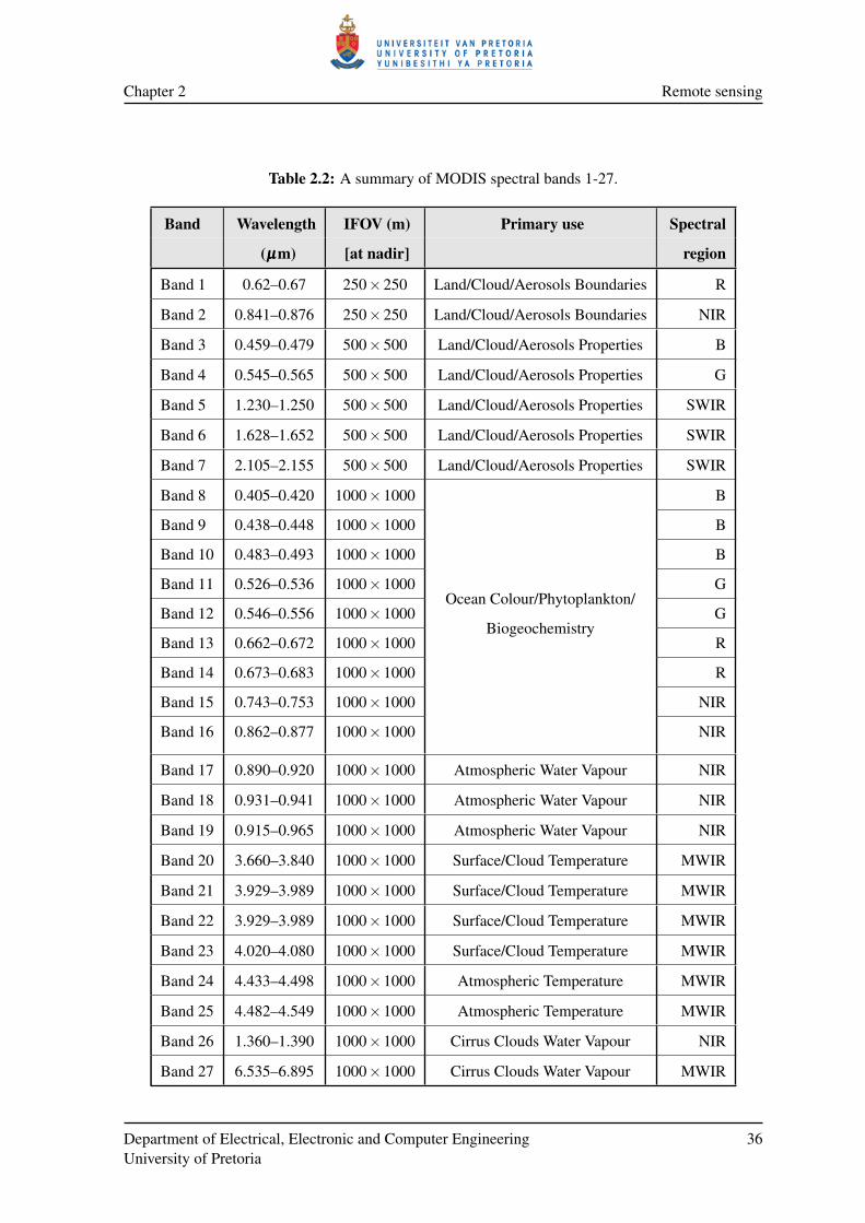
Chapter 2 Remote sensing
Table 2.2: A summary of MODIS spectral bands 1-27.
Band Wavelength IFOV (m) Primary use Spectral
(µµµm) [at nadir] region
Band 1 0.62–0.67 250×250 Land/Cloud/Aerosols Boundaries R
Band 2 0.841–0.876 250×250 Land/Cloud/Aerosols Boundaries NIR
Band 3 0.459–0.479 500×500 Land/Cloud/Aerosols Properties B
Band 4 0.545–0.565 500×500 Land/Cloud/Aerosols Properties G
Band 5 1.230–1.250 500×500 Land/Cloud/Aerosols Properties SWIR
Band 6 1.628–1.652 500×500 Land/Cloud/Aerosols Properties SWIR
Band 7 2.105–2.155 500×500 Land/Cloud/Aerosols Properties SWIR
Band 8 0.405–0.420 1000×1000
Ocean Colour/Phytoplankton/
B
Band 9 0.438–0.448 1000×1000
Biogeochemistry
B
Band 10 0.483–0.493 1000×1000 B
Band 11 0.526–0.536 1000×1000 G
Band 12 0.546–0.556 1000×1000 G
Band 13 0.662–0.672 1000×1000 R
Band 14 0.673–0.683 1000×1000 R
Band 15 0.743–0.753 1000×1000 NIR
Band 16 0.862–0.877 1000×1000 NIR
Band 17 0.890–0.920 1000×1000 Atmospheric Water Vapour NIR
Band 18 0.931–0.941 1000×1000 Atmospheric Water Vapour NIR
Band 19 0.915–0.965 1000×1000 Atmospheric Water Vapour NIR
Band 20 3.660–3.840 1000×1000 Surface/Cloud Temperature MWIR
Band 21 3.929–3.989 1000×1000 Surface/Cloud Temperature MWIR
Band 22 3.929–3.989 1000×1000 Surface/Cloud Temperature MWIR
Band 23 4.020–4.080 1000×1000 Surface/Cloud Temperature MWIR
Band 24 4.433–4.498 1000×1000 Atmospheric Temperature MWIR
Band 25 4.482–4.549 1000×1000 Atmospheric Temperature MWIR
Band 26 1.360–1.390 1000×1000 Cirrus Clouds Water Vapour NIR
Band 27 6.535–6.895 1000×1000 Cirrus Clouds Water Vapour MWIR
Department of Electrical, Electronic and Computer EngineeringUniversity of Pretoria
36

Chapter 2 Remote sensing
Table 2.3: A summary of MODIS spectral bands 28-36.
Band Wavelength IFOV (m) Primary use Spectral
(µµµm) [at nadir] region
Band 28 7.175–7.475 1000×1000 Cirrus Clouds Water Vapour LWIR
Band 29 8.400–8.700 1000×1000 Cloud Properties LWIR
Band 30 9.580–9.880 1000×1000 Ozone LWIR
Band 31 10.780–11.280 1000×1000 Surface/Cloud Temperature LWIR
Band 32 11.770–12.270 1000×1000 Surface/Cloud Temperature LWIR
Band 33 13.185–13.485 1000×1000 Cloud Top LWIR
Band 34 13.485–13.785 1000×1000 Cloud Top LWIR
Band 35 13.785–14.085 1000×1000 Cloud Top LWIR
Band 36 14.085–14.385 1000×1000 Cloud Top LWIR
Table 2.4: MODIS Design Specifications.
Orbit 705 km, 10:30 AM descending node or
1:30 PM ascending node, sun-synchronous,
near polar, circular
Scan rate 20.3 rpm, cross track
Swath dimension 2330 km (cross track) by 10 km (along track at nadir)
Telescope 17.78 cm off-axis, a focal (collimated),
with intermediately held stop
Size 1.0×1.6×1.0 m3.
Weight 250 kg
Power 225 W (orbital average)
Data rate 11 Mbps (peak daytime)
Quantisation 12 bits
Spatial resolution (at nadir) 250m (bands 1–2)
500m (bands 3–7), 1000 m (bands 8–36)
Design life 5 years
Department of Electrical, Electronic and Computer EngineeringUniversity of Pretoria
37

Chapter 2 Remote sensing
data from EOS-Terra, MYD indicates that data from EOS-Aqua was used and MCD indicates that the
product was generated using data from EOS-Terra and EOS-Aqua. Normally two numbers follow the
three letters and indicate the intended application of the product. A list of these numbers with their
appropriate descriptions can be found in Table 2.5 and Table 2.6.
Most standard MODIS land products use a sinusoidal grid tiling system. Tiles are 10 degrees by 10
degrees at the equator. The tile coordinate system starts at (0,0) (horizontal tile number, vertical tile
number) in the upper left corner and proceeds right (horizontal) and downward (vertical). The tile in
the bottom right corner is (35,17).
2.7.4 MODIS design
MODIS is a whiskbroom scanning radiometer with a double-sided paddle wheel scan mirror, which
operates at 20.3 rpm. The incident radiation (earth view) is reflected from the scan mirror to a fold
mirror. From the fold mirror the radiation is reflected onto the primary mirror of the Afocal Gregorian
Telescope. The radiation is reflected by the primary mirror and then passes through a field stop. After
passing through the field stop the radiation falls upon the secondary mirror of the telescope. The
secondary mirror then reflects the incident radiation to three dichroic beamsplitters. The beamsplitters
split the radiation into four regions: NIR, visible, SWIR and MWIR, and LWIR, after which the
radiation ends up on four Focal Plane Assemblies (FPAs), one for each region. The MODIS sensor
also houses four on-board calibrators. The name of each calibrator is given below [37, 38]:
1. Solar Diffuser (SD) and Solar Diffuser Stability Monitor (SDSM),
2. Spectral Radiometric Calibration Assembly (SRCA),
3. Blackbody (BB),
4. Space View (SV).
2.7.5 The MCD43A4 product
The MCD43A4 MODIS product consists of seven BRDF corrected land surface reflectance (eight-day
composite, 500 m resolution) time-series [22]. BRDF is discussed in Section 2.5.3. The reason for
selecting this product was discussed in Section 1.3. The product is built from a 16-day rolling window
Department of Electrical, Electronic and Computer EngineeringUniversity of Pretoria
38

Chapter 2 Remote sensing
Table 2.5: The MODIS Product Codes 01–28
Product Code# Description
01 Level-1A Radiance Counts
02 Level-1B Calibrated, Geolocated Radiances
03 Geolocation Data Set
04 Aerosol Product
05 Total Precipitable Water
06 Cloud Product
07 Atmospheric Profiles
08 Gridded Atmosphere Products (Level 3)
09 Atmospherically Corrected Surface Reflectance
10 Snow Cover
11 Land Surface Temperature and Emissivity
12 Land Cover/ Land Change
13 Vegetation Indices
14 Thermal Anomalies, Fires and Biomass Burning
15 Leaf Area Index and FPAR
16 Surface Resistance and Evapotranspiration
17 Vegetation Production, Net Primary Productivity
18 Normalised Water Leaving Radiance
19 Pigment Concentration
20 Chlorophyll II, Fluorescene
21 Chlorophyll and Pigment Concentration
22 Photosynthetically Active Radiation
23 Suspended Solids Concentration in Ocean Water
24 Organic Matter Concentration
25 Coccolith Concentration
26 Ocean Water Attenuation Coefficient
27 Ocean Primary Productivity
28 Sea Surface Temperature
Department of Electrical, Electronic and Computer EngineeringUniversity of Pretoria
39

Chapter 2 Remote sensing
Table 2.6: The MODIS Product Codes 29–MODISALB.
Product Code# Description
29 Sea Ice Cover
31 Phycoerythrin Concentration
35 Cloud Mask
36 Total Absorption Coefficient
36 Total Absorption Coefficient
37 Ocean Aerosol Properties
39 Clear Water Epsilon
43 Albedo-16 day (Level 3)
44 Vegetation Cover Conversion and Continuous Fields
MODISALB Snow and Sea Ice Albedo
of acquisitions obtained from the Terra and Aqua satellites, which explains the use of “MCD” in the
product name. An MCD43A4 pixel value consists of seven reflection ratios (at 500 m resolution).
The seven reflection ratios are located in the seven MODIS land bands. The raw MCD43A4 data are
DNs (16-bit unsigned integer values). The raw 16-bit data of MCD43A4 should not be confused with
the raw radiation value (which is a 12-bit value) recorded by the MODIS sensor. The raw MCD43A4
data should be multiplied by 0.0001 to obtain reflection ratios. The temporal period of MODIS
MCD43A4 (if an observation is produced every eight-days) roughly translates to 45 observations per
year. NDVI is calculated from MCD43A4 by using Equation 2.11. In the remainder of this thesis the
phrase “MODIS pixel” refers to the seven time-series at 500 m resolution that are associated with the
MCD43A4 product.
2.8 DATASET DESCRIPTION
The datasets used in this thesis are constructed from the eight-day composite MODIS MCD43A4
BRDF corrected 500 m land surface reflectance product. The study areas associated with the MODIS
MCD43A4 datasets span a total area of approximately 230 km2 in Gauteng and 800 km2 in Limpopo,
South Africa. Gauteng and Limpopo are provinces in South Africa and their physical location is
shown in Figure 2.12.
Department of Electrical, Electronic and Computer EngineeringUniversity of Pretoria
40

Chapter 2 Remote sensing
Gauteng is the smallest province in South Africa. The name “Gauteng” is derived from the Sesotho
word meaning “Place of Gold”. The name chosen for Gauteng is appropriate as it is the economic
heart of South Africa. The capital of Gauteng is Johannesburg [12].
Limpopo is the northernmost province of South Africa. It is named after the Limpopo River. “Lim-
popo” is the Zulu word for “waterfalls”. The Limpopo province houses the largest hunting industry in
the country. The capital of Limpopo is Polokwane and was formerly known as Pietersburg [12].
The reasons for selecting Gauteng and Limpopo as study regions were discussed in Section 1.1.
15 19 23 27 31 35-36
-34
-32
-30
-28
-26
-24
-22
Geographic longitude (degrees)
Geograp
hic
latitude(degrees)
Namibia
Botswana
Gauteng
Limpopo
Figure 2.12: The physical location of the Gauteng province and the Limpopo province [2] © IEEE
2012.
Two land cover classes are considered: settlements and natural vegetation, denoted by s and v res-
pectively. In this thesis the settlements class contains pixels that contain more than 50% buildings
(construction), whereas the vegetation class contains pixels with more than 90% vegetation.
The above class classification rule is illustrated below with an example. Figure 2.13 is a Google
EarthTM image of a populated area in Gauteng. Four red parallelograms are visible in Figure 2.13.
Each red parallelogram represents a pixel that is actually surveyed by the MODIS sensor and is
500 m×500 m in size. If the vegetation settlement classification rule mentioned above is applied to
Figure 2.13, only the bottom right pixel would be classified as a vegetation pixel, while the remaining
three would be classified as settlement pixels.
Two MODIS MCD43A4 datasets are used to investigate the hypertemporal techniques discussed in
Department of Electrical, Electronic and Computer EngineeringUniversity of Pretoria
41

Chapter 2 Remote sensing
Figure 2.13: A Google EarthTM image of a populated area in Gauteng (courtesy of Google EarthTM).
2001 2002 2003 2004 2005 2006 2007 2008 20090
5
10
15
20
25
30
35
4045
Band 1Band 2Band 3Band 4Band 5Band 6Band 7%
Refl
ecta
nce
Figure 2.14: A random vegetation MODIS pixel in Gauteng.
Department of Electrical, Electronic and Computer EngineeringUniversity of Pretoria
42

Chapter 2 Remote sensing
this thesis. The Gauteng dataset consists of 1106 MODIS pixels, while the Limpopo dataset contains
3349 MODIS pixels and was selected with visual (human) interpretation of two high-resolution SPOT
images from 2001 and 2009. MODIS pixels that, according to the SPOT images, either did not change
or changed from vegetation to settlement were selected. Each MCD43A4 MODIS pixel contains
seven time-series with I = 368 observations (extracted between January 2001 and March 2009).
An NDVI time-series can be added to a MODIS pixel and is computed using the first two spec-
tral land bands. The Gauteng and Limpopo datasets are respectively divided into the three classes:
natural vegetation (592 Gauteng pixels and 1497 Limpopo pixels), settlements (333 Gauteng pixels
and 1735 Limpopo pixels) and real land cover change from vegetation to settlement (181 Gauteng
pixels and 117 Limpopo pixels). A random vegetation MODIS pixel in Gauteng is displayed in Fi-
gure 2.14.
2.9 CONCLUSION
The chapter provided a broad overview of the remote sensing field, which included a brief history
of remote sensing, an introduction to the physical principles behind remote sensing, an overview of
remote sensing platforms and an introduction to the MODIS sensor. The MODIS data used by the
classification and change detection algorithms investigated in this thesis were also presented in this
chapter.
Department of Electrical, Electronic and Computer EngineeringUniversity of Pretoria
43

CHAPTER 3
SEQUENTIAL ANALYSIS
The main reason for including this chapter in the thesis is to provide the theoretical background
knowledge required to implement CUSUM as a sequential hypertemporal remote sensing change
detection algorithm. It is recommended to first study Section A.1 if the reader is unfamiliar with
stochastic calculus. Stochastic calculus provides the mathematical framework needed to understand
and study sequential analysis.
In this chapter, different statistical techniques are investigated either to classify observations or to
detect changes in the underlying distribution of observation. All the techniques investigated have no
pre-determined sample size and are thus purely sequential or on-line. The study of statistical sequen-
tial classification and change detection techniques is known collectively as sequential analysis. Good
literature reviews can be found in [24, 25] on the subject of sequential analysis. The main advantage
of a sequential approach is that on average sequential approaches require fewer observations than a
fixed-sample-size approach while maintaining the same probability of error. The reason for this is
that sequential algorithms terminate uniquely for each observable sequence. In an ambiguous case
the algorithm will take longer to terminate than in an unambiguous case [23]. The chapter starts with
Neyman and Pearson’s 1933 seminal result [44], which provides an optimal fixed-sample-size classi-
fication strategy. Neyman and Pearson’s result inspired Wald [45,46] to develop a sequential solution
to the classification problem during the 1940s. Optimality was subsequently proven by Wald and
Wolfowitz in 1948 [47]. The sequential classification problem, also known as sequential detection, is
discussed in two frameworks, namely in Wald’s framework (frequentest) (Section 3.3) [46] and in a
Bayesian framework (Section 3.4) [48]. From sequential detection the chapter progresses to a group
of change detection algorithms grouped under the collective name of quickest detection. Quickest
detection techniques are statistical techniques capable of detecting a change as quickly as possible

Chapter 3 Sequential analysis
after it occurs (using different measures for the delay). Statistical change detection has its roots in the
seminal papers of Shewhart [49] and Page [6]. The quickest detection techniques discussed in this
chapter are divided into Bayesian (see Section 3.5) and non-Bayesian (see Section 3.6) approaches.
The problem of quickest detection was first cast into a Bayesian framework in 1952 [50], and was
subsequently solved in 1963 by Shiryaev [51]. The most famous non-Bayesian change detection al-
gorithm is arguably the CUSUM stopping time, first developed by Page (see Section 3.6.1) [6]. It has
been shown that the CUSUM stopping time is asymptotically optimal [52] (when employing the worst
case expected delay as a performance measure). The asymptotically optimal result was later extended
by showing that the CUSUM stopping time is in fact exactly optimal [53, 54]. An alternative to the
CUSUM stopping rule was proposed in 1966 and is known as the Shiryaev-Roberts stopping time (see
Section 3.6.2) [51, 55]. An extension to the Shiryaev-Roberts stopping time known as the Shiryaev-
Roberts-Pollak stopping time was developed in 1985 by Pollak [56]. The Shiryaev-Roberts-Pollak
method is a third-order asymptotically optimal sequential procedure when employing Pollak’s perfor-
mance measure (which is less restrictive than the worst case expected delay) [56]. More recently the
Shiryaev-Roberts-Pollak stopping time was extended to the deterministic Shiryaev-Roberts stopping
time [57, 58], which can uniformly outperform both Shiryaev-Roberts and Shiryaev-Roberts-Pollak
for appropriately chosen starting conditions [57,58]. For a good theoretical introduction to sequential
analysis the reader is referred to [48], while the reader is referred to [59] for an overview that focuses
more strongly on implementation specifics.
3.1 NEYMAN-PEARSON
The following section closely follows the notation of [60, 61]. Let zn = zkk=1,2,··· ,n be an inde-
pendent and identically distributed (i.i.d.) sequence of real observation of size n following one of two
hypotheses:
H0 : zk ∼ Q0, k = 1,2, · · · ,n
versus
H1 : zk ∼ Q1, k = 1,2, · · · ,n;
where Q0 and Q1 are two probability distributions with associated densities q0 and q1, respectively.
The problem is to determine which hypothesis is true by only looking at the observations. Fur-
thermore, let q0(zn) and q1(zn) denote n-dimensional density functions. Let T be a function of the
observations, known as the test statistic and let R be the image of T . The image R can be divided into
Department of Electrical, Electronic and Computer EngineeringUniversity of Pretoria
45

Chapter 3 Sequential analysis
a critical region R0 and a region of acceptance R1, such that R0 ∪R1 = R. If T (zn) fall into R0, H0
is rejected. Constructing a hypothesis test thus requires selecting a test statistic and a critical region.
The probability α of rejecting H0 when it is in fact true is known as the level of significance or the
size of the test and is equal to
α =∫
zn:T (zn)∈R0q0(zn)dzn.
The probability α is also known as the probability of a false alarm PFA or the type I error. The power
of the test 1−β is defined as the probability of accepting H1 if it is in fact true, also known as the
probability of detection PD, and is equal to
1−β =∫
zn:T (zn)∈R0q1(zn)dzn.
In other words, β is the probability of accepting H0 when it is in fact false (type II error).
Neyman and Pearson [44, 61] derived the following theorem, which states that the likelihood ratio Λ
is the best possible choice of T . The likelihood ratio maximises the PD given a specific false alarm
rate PFA.
Theorem 1 (Neyman-Pearson) To maximise the PD for a given PFA decide H1 if
Λ(zn) =q1(zn)
q0(zn)> γ,
where the threshold γ is found from
PFA =∫
zn:Λ(zn)>γq0(zn)dzn.
3.2 KULLBACK-LEIBLER DIVERGENCE
Theorem 1 stipulates that Λ is the optimal test statistic and some of the unique properties of Λ that
make it a useful tool when building a classifier or a change detector should therefore be highlighted.
Instead of calculating the likelihood ratio
Λk =k
∏i=1
q1(zi)
q0(zi), (3.1)
the log-likelihood ratio
Sk =k
∑i=1
si, (3.2)
where
si = lnq1(zi)
q0(zi), (3.3)
Department of Electrical, Electronic and Computer EngineeringUniversity of Pretoria
46

Chapter 3 Sequential analysis
could be calculated. The sum Sk is derived from lnΛk.
In probability theory and information theory, the Kullback-Leibler divergence is a non-symmetric
measure of the difference between two probability distributions Q0 and Q1 and is defined as
DKL(Q1‖Q0) =∫
∞
−∞
q1(z1)lnq1(z1)
q0(z1)dz1
= E1
[ln
q1(z1)
q0(z1)
]
= E1[s1].
The reason why z1 can be used is that the sequence z = zkk=1,2,··· is a sample path of a discrete,
stationary stochastic process. In other words, the density of the first observation of multiple sample
paths equals the density from which the sequence z is drawn. Kullback-Leibler divergence is always
positive, implying that Sk will have positive drift under H1, because E1[s1] > 0. Under H0, Sk will
have negative drift, since E0[s1] =−∫
∞
−∞q0(z)ln
q0(z)q1(z)
dz =−DKL(Q0‖Q1)< 0. It should be perfectly
clear that lnΛ is a good statistic to use when building a classifier, since under H1, Sk experiences
positive drift, while under H0, Sk experiences negative drift [59].
3.3 HYPOTHESIS TESTING: WALD’S FORMULATION
The following section closely follows the notation of [59]. The problem with Neyman-Pearson is that
the sample size has to be chosen before the threshold can be computed and therefore the algorithm
is non-sequential. In contrast with Neyman-Pearson, Wald’s formulation, the Sequential Probability
Ratio Test (SPRT), is a sequential approach and is the Uniformly Most Efficient (UME) test among
all sequential tests. In general the art of classifying as quickly (no predetermined sample size) and
accurately as possible is known as sequential detection.
The problem introduced in Section 3.1 is now restated without limiting the sample size. Consider the
sequence z = zkk=1,2,··· of i.i.d. real observation following one of two hypotheses:
H0 : zk ∼ Q0, k = 1,2, · · ·
versus
H1 : zk ∼ Q1, k = 1,2, · · · ;
where Q0 and Q1 are two probability distributions with associated densities q0 and q1, respectively.
Department of Electrical, Electronic and Computer EngineeringUniversity of Pretoria
47

Chapter 3 Sequential analysis
Furthermore, let the sequence z be adapted to the filtration Fk = σ(zkk=1,2,···). The problem is to
determine which hypothesis is true by only looking at the observations.
The above problem can be solved by using a sequential statistical test. A sequential statistical test
for testing between hypotheses H0 and H1 is defined by a sequential decision rule, which is the pair
(δ ,T ), where T is a stopping time and δ a decision function. In the case of the SPRT the stopping
time is equal to
T = T SPRTA,B = infk ≥ 0|Λk /∈ (A,B), (3.4)
where Λk was defined in Equation 3.1, and the decision function (after stopping) is
δT =
0 when ΛT ≤ A
1 when ΛT ≥ B.
In other words, Wald’s test keeps on sampling until the likelihood ratio crosses the exit thresholds
A or B, at which time a decision is made. If ΛT is less or equal to A, hypothesis H0 is accepted, if
ΛT is greater or equal to B, hypothesis H1 is accepted. The type I error α is equal to the probability
P0(δT = 1), where the subscript refers to the fact that H0 is assumed to be true. The probability of a
type II error β is equal to the probability P1(δT = 0).
The log-likelihood ratio Sk (Equation 3.2) can also be used instead of Λk to derive the sequential
decision rule, (δ ,T ). In the log-likelihood domain the SPRT stopping time is equal to
T = T SPRT−a,h = infk ≥ 0|Sk /∈ (−a,h), (3.5)
where lnA =−a and lnB = h. The decision rule now becomes
δT =
0 when ST ≤−a
1 when ST ≥ h.
Overshoot is an important concept that is often used to analyse the performance of the SPRT algorithm
and should therefore be defined formally. Let
O(T,ST ,−a,h,δT ) =
|ST +a| when δT = 0
|ST −h| when δT = 1.(3.6)
When inspecting Equation 3.6 it should be clear to the reader that O(T,ST ,−a,h,δT ) is a random
variable. If O(T,ST ,−a,h,δT )≡ 0 then there is no overshoot (ST always equals one of the boundaries
a,h), however when O(T,ST ,−a,h,δT ) 6≡ 0 then overshoot does occur.
Department of Electrical, Electronic and Computer EngineeringUniversity of Pretoria
48

Chapter 3 Sequential analysis
As mentioned before, Wald’s SPRT is the UME test among all sequential tests. This fact is formally
stated by the Wald-Wolfowitz theorem, given below without proof [47, 48].
Theorem 2 (Wald-Wolfowitz) Suppose (T,δ ) is the Sequential Probability Ratio Test, SPRT(A,B)
with 0 < A ≤ 1 ≤ B < ∞, and let (T ′,δ ′) denote any other sequential decision rule with
maxE0[T ′],E1[T ′]< ∞, and satisfying
α′ = P0(δ
′T ′ = 1)≤ P0(δT = 1) = α and β
′ = P1(δ′T ′ = 0)≤ P1(δT = 0) = β ,
with
P0(δT = 1)+P1(δT = 0)< 1.
Then
E0[T ′]≥ E0[T ] and E1[T ′]≥ E1[T ].
At this point the natural question arises, “How can the thresholds A and B be selected to achieve a
certain probability of error?” It turns out that it is quite complex to find the exact thresholds A and
B, but quite simple to find approximations of A and B that typically work well in practice. These
practical estimates are known as Wald’s approximations of A and B. When Λk ≥ B, sampling stops
and hypothesis H1 is chosen. Clearly the decision rule leads to [23]
k
∏i=1
q1(zk)≥ B ·k
∏i=1
q0(zk) =⇒ P1(δ = 1)≥ B ·P0(δ = 1), (3.7)
which can be interpreted as the probability of observing zk under H1 is at least B times bigger than
under H0. Furthermore, since H1 was chosen, the type I error is equal to P0(δ = 1). Recognising
the type II error β to be equal to P1(δ = 0), an upper limit for B can be derived by using Equation 3.7
and is equal to
B≤ 1−β
α. (3.8)
Similarly a lower limit for A can be derived and is equal to
A≥ β
1−α. (3.9)
Wald’s approximations for A and B are derived by replacing the inequalities with equalities in Equa-
tion 3.9 and Equation 3.8 and are thus equal to
A =β
1−αand B =
1−β
α.
Department of Electrical, Electronic and Computer EngineeringUniversity of Pretoria
49

Chapter 3 Sequential analysis
Wald’s approximations for the log-likelihood domain can be found similarly and are equal to
−a = lnβ
1−αand h = ln
1−β
α.
Alternatively Wald’s approximate error probabilities can be calculated with the correct exit bounda-
ries A and B, resulting in
α =1−AB−A
and β = AB−1B−A
. (3.10)
3.3.1 The OC and ASN functions of the SPRT
The problem stated at the beginning of Section 3.3 is restated with additional information to help
in defining the Operating Characteristic (OC) and the Average Sample Number (ASN) functions
properly. Consider the sequence z = zkk=1,2,··· of i.i.d. real observations (adapted to the filtration
Fk), which obeys one of the two hypotheses,
H0 : θ = θ0
versus
H1 : θ = θ1;
best, where θ ∈Θ is a unique property of the random variable generating the sequence z, for example
θ could represent the mean of a Gaussian random variable and Θ ⊂ R is the possible range of θ .
The problem could also be stated for a parameter list θθθ , but for simplicity it is not done here. If θ
is equal to θ0, the random variable generating the sequence z will obey density q0, similarly when θ
equals θ1 the sequence z will be distributed according to density q1. Assume now that the sequence s
is derived from z by using Equation 3.3 and is also i.i.d.. Under H0 the random variable generating
s will have density f0 and under H1 the random variable will have density f1, which is shorthand for
fθ0 and fθ1 , respectively. In general, when the unique property of z is equal to θ , the sequence s will
be distributed according to density fθ . In effect the parameter θ determines the density of the random
variable generating s.
The probability Q(θ) of accepting hypothesis H0, treated as a function of θ ∈ Θ, when the exit
thresholds −a and h are fixed, is called the operating characteristic function. In other words the type
I error α is equal to 1−Q(θ0) and the type II error β is equal to Q(θ1) [59].
The average sample number Eθ [T ] is the mean number of sample points required to make a decision
when performing a hypothesis test, with fixed exit thresholds −a and h, as a function of θ ∈ Θ . In
Department of Electrical, Electronic and Computer EngineeringUniversity of Pretoria
50

Chapter 3 Sequential analysis
the cases where θ equals θ0 or θ1 the shorthand notations E0[T ] and E1[T ] are used. If the sequence
z follows H0, the expected number of samples required to make a decision is equal to E0[T ], while
E1[T ] is defined similarly [59].
3.3.2 Wald’s approximations
The OC function Q(θ) can be approximated by Q(θ) with equation
Q(θ) =
e−ω0(θ)h−1e−ω0(θ)h−eω0(θ)a
when Eθ [s1] 6= 0
hh+a when Eθ [s1] = 0,
(3.11)
where ω0(θ) is the unique non-zero real number which satisfies
Eθ [e−ω0(θ)s1 ] =∫
∞
−∞
e−ω0(θ)s1 fθ (s1)ds1 (3.12)
= 1,
if a non-zero solution exists, otherwise ω0(θ) = 0, and Eθ [s1] is defined as
Eθ [s1] =∫
∞
−∞
s1 fθ (s1)ds1. (3.13)
Wald’s approximation of Q(θ) is derived from the following well-known identity of Wald (see Theo-
rem 6) [48]
Eθ
[e−ωST
(Eθ
[e−ωs1
])−T ]= 1, (3.14)
where T is the SPRT stopping time defined in Equation 3.5. Wald’s identity is valid for all ω ∈ω|Eθ [e−ωs1 ]< ∞. Equation 3.14 can be transformed into
Eθ
[e−ωST−T lnEθ [e−ωs1 ]
]= 1, (3.15)
trivially. If ω is substituted with ω0(θ), Equation 3.15 reduces to
Eθ
[e−ω0(θ)ST
]= 1. (3.16)
If the excess over the boundaries −a and h is ignored, ST is approximately equal to either −a or h,
and Equation 3.16 becomes
e−ω0(θ)h[1−Pθ (ST ≤−a)]+ eω0(θ)aPθ (ST ≤−a)≈ 1, (3.17)
Department of Electrical, Electronic and Computer EngineeringUniversity of Pretoria
51

Chapter 3 Sequential analysis
where Pθ (ST ≤−a) is equal to Q(θ). By making Q(θ) the subject of Equation 3.17, Equation 3.11
is obtained.
The ASN function Eθ (T ) can be approximated via Eθ (T ) with equation
Eθ [T ] =
−aQ(θ)+h(1−Q(θ))Eθ [s1]
when Eθ [s1] 6= 0
a2Q(θ)+h2(1−Q(θ))
Eθ [s21]
when Eθ [s1] = 0.(3.18)
The approximation of the ASN function was also derived through another identity of Wald, na-
mely
Eθ [T ] =
Eθ [ST ]Eθ [s1]
if E[s1] 6= 0
Eθ [S2T ]
Eθ [s21]
if E[s1] = 0,(3.19)
where Eθ [ST ] equals
−aQ(θ)+h[1− Q(θ)], (3.20)
and Eθ [S2T ] equals
a2Q(θ)+h2[1− Q(θ)], (3.21)
if the excess over the boundaries is ignored. The stopping time T used in Wald’s identity is again the
SPRT stopping time in Equation 3.5. The result of substituting Equation 3.20 and Equation 3.21 into
Equation 3.19 is Equation 3.18.
Wald’s approximations can be restated in the likelihood domain in which case Q(θ) and Eθ [T ] can
be expressed as
Q(θ) =
B−ω0(θ)−1B−ω0(θ)−A−ω0(θ)
when Eθ (s1) 6= 0
lnBln(BA−1)
when Eθ (s1) = 0,
and
Eθ [T ] =
lnAQ(θ)+lnB(1−Q(θ))Eθ [s1]
when Eθ [s1] 6= 0
(lnA)2Q(θ)+(lnB)2(1−Q(θ))
Eθ [s21]
when Eθ [s1] = 0.
In the special case when θ = θ0 or θ = θ1 then Q(θ0) and Q(θ1) reduces to
Q(θ0) =B−1B−A
and Q(θ1) = AB−1B−A
,
Department of Electrical, Electronic and Computer EngineeringUniversity of Pretoria
52

Chapter 3 Sequential analysis
respectively, which is nothing more than the approximations already stated in Equation 3.10. The
function Eθ (T ) also simplifies in the two special cases θ = θ0 and θ = θ1 to
E0[T ] = (E0[s1])−1[
α ln(
1− β
α
)+(1− α) ln
(β
1− α
)], (3.22)
E1[T ] = (E1[s1])−1[(1− β ) ln
(1− β
α
)+ β ln
(β
1− α
)], (3.23)
respectively, where α and β are Wald’s probability of error approximations [59].
3.3.3 Exact computation
For a given θ , let Pθ (−a|y) = Pθ (y) be the probability that Sk (Equation 3.2), starting from y, reaches
the lower bound −a, and let Eθ [T |y] = Nθ (y) be the expected number of sample points required by
the SPRT algorithm to terminate when Sk starts at y, i.e. Sk = ∑ki=1 si + y [59]. It should now be clear
that Q(θ) is equal to Pθ (0) and Eθ [T ] is equal to Nθ (0). It is widely known that Pθ (y) and Nθ (y)
respectively satisfy the following two Fredholm integral equations of the second kind [62],
Pθ (y) =∫ −a−y
−∞
fθ (s1)ds1 +∫ h
−aPθ (s1) fθ (s1− y)ds1, −a≤ y≤ h, (3.24)
Nθ (y) = 1+∫ h
−aNθ (s1) fθ (s1− y)ds1, −a≤ y≤ h, (3.25)
which can be solved through a system of linear equations that approximate Equation 3.24 and Equa-
tion 3.25 [63]. The derivation of Pθ (y) and Nθ (y) is based upon the theory of a random walk with
absorbing and reflecting boundaries (barriers) [59]. See Section 3.3.5.2 for further details. Another
exact approach is the Markov method of Brook [64].
3.3.4 Simulation
The easiest way to compute Q(θ) and Eθ [T ] is through simulation. The pseudo-code for computing
the OC and ASN functions is given in Listing 3.1 (listed at the end of the chapter). The functions
obtained via simulation become more accurate as N becomes larger.
3.3.5 Example: Gaussian random variable
Consider the sequence z = zkk=1,2,··· of i.i.d. real observations (adapted to the filtration Fk) ge-
nerated by a Gaussian random variable with density N (θ ,1). The problem is to choose one of two
Department of Electrical, Electronic and Computer EngineeringUniversity of Pretoria
53

Chapter 3 Sequential analysis
fixed hypotheses so that the data sequence fits that hypothesis best. The following two hypotheses are
under consideration:
H0 : θ = θ0 = 0
versus
H1 : θ = θ1 = 1.
For this example the increment sequence s becomes skk=1,2,··· = zk− 12k=1,2,···, since
sk = lnq1(zk)
q0(zk)
= lne−(zk−1)2
e−z2k
= zk−12,
and is thus also an independent Gaussian sequence with density fθ (s1) =1√2π
e−(s1−(θ− 1
2 ))2
2 . Example
realisations of zk and Sk when θ = θ0 or θ = θ1 are given in Figure 3.1, while the probability density
functions of the random variable generating zk and sk under the same assumption of θ are given in
Figure 3.2. Note that the example sequences are classified correctly for the exit thresholds equal to
h = 3 and −a = −3 and that the stopping times are equal to T = 15 and T = 11 in Figure 3.1c and
Figure 3.1d, respectively.
The OC and ASN functions offer insight into the problem given above and will be calculated by using
Wald’s approximation as well as the exact computational approach presented in Section 3.3.3.
3.3.5.1 Wald’s approximation
The first step in calculating the OC and ASN functions is to determine ω0(θ) by using Equation 3.12
and for this example is equal to
E[e−ω0(θ)s1 ] =∫
∞
−∞
e−ω0(θ)s11√2π
e−(s1−(θ− 1
2 ))2
2 ds1
= 1
e−ω0(θ)(θ− 12 )+
12 ω2
0 (θ) = e0
ω0(θ) = 2θ −1. (3.26)
The next step is to calculate Eθ [s1] by using Equation 3.13, in order to attain
Eθ [s1] = θ − 12.
Department of Electrical, Electronic and Computer EngineeringUniversity of Pretoria
54

Chapter 3 Sequential analysis
1 5 10 15-2
-1.5
-1
-0.5
0
0.5
1
1.5
2
2.5
3
H0 : θ = 0
H1 : θ = 1
k
z k
(a) zk under H0.
1 5 10 11-2
-1.5
-1
-0.5
0
0.5
1
1.5
2
2.5
3
H0 : θ = 0
H1 : θ = 1
k
z k
(b) zk under H1.
1 5 10 15-5
-4
-3
-2
-1
0
1
2
3
4
5
h
−a
k
Sk
T = 15
Accept H0
Accept H1
(c) Sk under H0.
1 5 10 11-5
-4
-3
-2
-1
0
1
2
3
4
5
h
−a
k
Sk
T = 11
Accept H0
Accept H1
(d) Sk under H1.
Figure 3.1: Example sequences of zk and Sk for the unit variance Gaussian example having a mean
of θ0 = 0 and θ1 = 1 under H0 and H1, respectively. The exit thresholds are equal to 3 and -3.
The quantity Eθ [s21] is also required and is equal to 1 since s2
1 ∼ χ21 . The approximate OC function is
determined by substituting Equation 3.26 into Equation 3.11 to obtain
Q(θ) =
e−(2θ−1)h−1e−(2θ−1)h−e(2θ−1)a when θ 6= 1
2
hh+a when θ = 1
2 .
(3.27)
Wald’s approximated OC function for the Gaussian example is presented in Figure 3.3.
The approximate ASN function is calculated by substituting Eθ [s1], Eθ [s21] and Equation 3.27 into
Department of Electrical, Electronic and Computer EngineeringUniversity of Pretoria
55

Chapter 3 Sequential analysis
-4 -3 -2 -1 0 1 2 3 4 50
0.1
0.2
0.3
0.4
0.5
zk under H0 and H1
Likelihood
q0 q1
(a) Probability density function of zk.
-4 -3 -2 -1 0 1 2 3 4 5
0.1
0.2
0.3
0.4
0.5
sk under H0 and H1
Likelihood
f0 f1
0
(b) Probability density function of sk.
Figure 3.2: Probability density functions of the random variable generating zk and sk under H0 and
H1.
Equation 3.18, which gives
Eθ [T ] =
1θ− 1
2
[1−ea(2θ−1)
e−h(2θ−1)−ea(2θ−1) h− e−h(2θ−1)−1e−h(2θ−1)−ea(2θ−1) a
]when θ 6= 1
2
ah when θ = 12 .
Wald’s approximated ASN function for the Gaussian example is presented in Figure 3.4.
3.3.5.2 Exact computation
By substituting fθ (s1) into Equation 3.24 and Equation 3.25 and applying the method of Gaussian
quadrature (Section A.2) [63, 65], Equation 3.24 and Equation 3.25 can be reduced to
P(y) = Φ
(−a− y−
(θ − 1
2
))+
m
∑k=1
Ak · (2π)−12 e−
12 (yk−y−(θ− 1
2 ))2 · P(yk), (3.28)
N(y) = 1+m
∑k=1
Ak · (2π)−12 e−
12 (yk−y−(θ− 1
2 ))2 · N(yk), (3.29)
where Φ(y) = (2π)−12∫ y−∞
e−t22 dt, and, Ak and yk are, respectively, the weights and roots of the Gaus-
sian quadrature for the interval [−a,h]. The θ subscript is dropped to avoid clutter. Equation 3.28 can
be replaced by the following system of linear equations
A · P = B,
Department of Electrical, Electronic and Computer EngineeringUniversity of Pretoria
56

Chapter 3 Sequential analysis
-1 -0.5 0 0.5 1 1.5 20
0.1
0.2
0.3
0.4
0.5
0.6
0.7
0.8
0.9
1
θ
Q(θ)orQ(θ)
Wald’s Approximation
Exact Computation
Simulation1− α
β
Figure 3.3: The exact OC function and Wald’s approximated OC function for the unit variance
Gaussian example with mean θ = 0 and θ = 1 under H0 and H1 respectively. The exit thresholds
are equal to 3 and -3.
-1 -0.5 0 0.5 1 1.5 20
2
4
6
8
10
12
14
θ
E θ[T]or
E θ[T]
Wald’s Approximation
Exact Computation
Simulation
Eθ0 [T ] Eθ1 [T ]
Figure 3.4: The exact ASN function and Wald’s approximated ASN function for the unit variance
Gaussian example with mean θ = 0 and θ = 1 under H0 and H1 respectively. The exit thresholds
are equal to 3 and -3.
Department of Electrical, Electronic and Computer EngineeringUniversity of Pretoria
57

Chapter 3 Sequential analysis
where the matrix A(m×m) and column vectors P(m×1) and B(m×1) are defined by
A = (ai j), i, j = 1, · · · ,m;
PT = [P(y1), · · · , P(ym)],
BT =
[Φ
(−a− y1−
(θ − 1
2
)), · · · ,Φ
(−a− ym−
(θ − 1
2
))],
with
ai j =−A jψ(y j,yi) for i 6= j,
aii = 1−Aiψ(y j,yi),
ψ(y j,yi) =1√2π
e−(y j−yi−(θ− 1
2 ))2
2 .
The column vector P can now be solved easily with P = A−1 · B. The OC function Q(θ) is obtained
by substituting the column vector P into Equation 3.28 and setting y to naught. Similarly, N can be
ascertained by replacing Equation 3.29 with the linear system
A · N = I,
where A is as before, I is an m×1 unit vector and N is the column vector NT = [N(y1), · · · , N(ym)].
As before, the column vector N can be solved with N = A−1 · I. The ASN function Eθ [T ] is obtained
by substituting the column vector N into Equation 3.29 and setting y to naught. The exact OC and
ASN functions for the Gaussian example are presented in Figure 3.3 and Figure 3.4. Note that the
curve obtained through simulation fits precisely on the exact theoretical curve.
The exact OC and ASN functions can be used to do a sweep of the exit boundaries. The type I and
type II error, as well as the ASN of the SPRT algorithm, are presented in Figure 3.5 for the unit
variance Gaussian example with exit boundaries in the range of [1,3].
3.3.6 Example: Bernoulli random variable
Consider the sequence z = zkk=1,2,··· of i.i.d. real observations (adapted to the filtration Fk) ge-
nerated by a Bernoulli random variable with probability mass function
qp(z1) =
p if z1 = 1
1− p if z1 = 0.
Department of Electrical, Electronic and Computer EngineeringUniversity of Pretoria
58

Chapter 3 Sequential analysis
0.035953
0.0359530.035953
0.0495780.049578
0.049578
0.0632020.063202
0.063202
0.0768260.076826
0.076826
0.0904510.090451
0.090451
0.104080.10408
0.10408
0.11770.1177
0.1177
0.13132
0.131320.13132
0.144950.14495
0.14495
0.158570.15857
0.15857
0.17220.1722
0.17220.18582
-3 -2.8 -2.6 -2.4 -2.2 -2 -1.8 -1.6 -1.4 -1.2 -11
1.2
1.4
1.6
1.8
2
2.2
2.4
2.6
2.8
3
h
−a
α
(a) Type I error.
0.035953
0.035953
0.049578
0.049578
0.063202
0.063202
0.076826
0.076826
0.090451
0.090451
0.10408
0.104080.10408
0.1177
0.11770.1177
0.13132
0.131320.13132
0.14495
0.144950.14495
0.15857
0.158570.158570.1722
0.17220.18582
0.18582
-3 -2.8 -2.6 -2.4 -2.2 -2 -1.8 -1.6 -1.4 -1.2 -11
1.2
1.4
1.6
1.8
2
2.2
2.4
2.6
2.8
3
−a
h
β
(b) Type II error.2.7325
3.092
3.092
3.4515
3.4515
3.4515
3.811
3.811
3.811
4.1705
4.1705
4.1705
4.53
4.53
4.53
4.8895
4.8895
4.8895
5.249
5.249
5.249
5.6085
5.6085
5.6085
5.968
5.968
6.3275
6.3275
6.687
-3 -2.8 -2.6 -2.4 -2.2 -2 -1.8 -1.6 -1.4 -1.2 -11
1.2
1.4
1.6
1.8
2
2.2
2.4
2.6
2.8
3
−a
h
Eθ0[T ]
(c) Eθ0 [T ].
2.7325
3.092
3.092
3.4515
3.4515
3.4515
3.811
3.811
3.811
4.1705
4.1705
4.1705
4.53
4.53
4.53
4.53
4.8895
4.8895
4.8895
5.249
5.249
5.249
5.249
5.6085
5.6085
5.6085
5.968
5.968
5.968
6.3275
6.3275
6.687
-3 -2.8 -2.6 -2.4 -2.2 -2 -1.8 -1.6 -1.4 -1.2 -11
1.2
1.4
1.6
1.8
2
2.2
2.4
2.6
2.8
3
−a
h
Eθ1[T ]
(d) Eθ1 [T ].
Figure 3.5: The general performance of the unit variance Gaussian example with mean θ = 0 and
θ = 1 under H0 and H1, respectively, and exit boundaries in the range of [1,3].
The problem is to choose one of two fixed hypotheses so that the data sequence fits that hypothesis
best. The following two hypotheses are under consideration:
H0 : p = p0 = y = 0.4
versus
H1 : p = p1 = 1− y = 0.6.
For this example the increment sequence s becomes
sk =
ln 1−yy if zk = 1
ln y1−y if zk = 0,
Department of Electrical, Electronic and Computer EngineeringUniversity of Pretoria
59

Chapter 3 Sequential analysis
with probability mass function equal to
fp(s1) =
p if s1 = ln 1−yy
1− p if s1 = ln y1−y .
and is thus also an i.i.d. Bernoulli sequence. To make the meaning of the OC and ASN functions
clearer, they will be calculated in the following sections by using Wald’s approximation, which for
the above problem also produces the exact solution. The series Sk can only increase or decrease by
ln 1−yy or − ln 1−y
y and as such if the exit thresholds are chosen as integer multiples of ln 1−yy there will
be no overshoot. When there is no overshoot, Wald’s approximations are exact as they are derived by
ignoring the overshoot.
3.3.6.1 Wald’s approximation
As stated before, the first step in calculating the OC and ASN functions is to determine ω0(p) by
using Equation 3.12. By applying Equation 3.12 the following is attained:
E[e−ω0(p)s1 ] = e−ω0(p)·ln 1−yy · p+ e−ω0(p)·ln y
1−y · (1− p)
= e−Y · p+ eY · (1− p) (3.30)
= 1.
Equation 3.30 can be solved by using a simple substitution, namely eY =X , as is done below:
e2Y · (1− p)− eY + p = 0
X 2 · (1− p)−X + p = 0.
The usable value of X (p) is equal to
X (p) =
1+√
1−4(1−p)·p2(1−p) if 0 < p≤ 0.5
1−√
1−4(1−p)·p2(1−p) if 0.5 < p < 1
(3.31)
and is a direct result of the quadratic formula. From Equation 3.31, ω0(p) is obtained trivially, as
eω0(p)·ln 1−yy is equal to X (p) so that
ω0(p) =lnX (p)
ln 1−yy
if 0 < p < 1
ω0(p)≈ 2.47lnX (p). (3.32)
Department of Electrical, Electronic and Computer EngineeringUniversity of Pretoria
60

Chapter 3 Sequential analysis
0 0.1 0.2 0.3 0.4 0.5 0.6 0.7 0.8 0.9 10
0.1
0.2
0.3
0.4
0.5
0.6
0.7
0.8
0.9
1Wald’s Approximation
Simulation
p
Q(p)
Figure 3.6: The exact OC function derived using Wald’s approximation for the Bernoulli example
with p0 = 0.4 and p1 = 0.6 under H0 and H1 respectively. The exit thresholds are equal to 8 ln 0.60.4
and −8ln 0.60.4 .
Note that when p→ 0, ω0(p)→−∞ and when p→ 1, ω0(p)→ ∞.
The OC function is calculated by substituting Equation 3.32 into Equation 3.11 to obtain
Q(p) =
e−2.47lnX h−1e−2.47lnX h−e2.47lnX a when p 6= 1
2
hh+a when p = 1
2 ,
(3.33)
and is presented in Figure 3.6. Note that the p of X (p) is implied.
The values Ep[s1] and Ep[s21] need to be calculated before computing the ASN function. For this
example, Ep[s1] = (2p+1) ln 1−yy ≈ 0.41(2p+1) and Ep[s2
1] = (ln 1−yy )2 ≈ 0.16. The ASN function
is calculated by substituting Ep[s1], Ep[s21] and Equation 3.33 into Equation 3.18 which gives
Ep[T ] =
10.41(2p+1)
[1−e2.47lnX a
e−2.47lnX h−e2.47lnX a h− e−2.47lnX h−1e−2.47lnX h−e2.47lnX a a
]when p 6= 1
2
ah0.16 when p = 1
2 .
The exact ASN function for the Bernoulli example can be found in Figure 3.7.
Department of Electrical, Electronic and Computer EngineeringUniversity of Pretoria
61

Chapter 3 Sequential analysis
0 0.1 0.2 0.3 0.4 0.5 0.6 0.7 0.8 0.9 10
10
20
30
40
50
60
70Wald’s Approximation
Simulation
p
E p[T]
Figure 3.7: The exact ASN function function derived using Wald’s approximation for the Bernoulli
example with p0 = 0.4 and p1 = 0.6 under H0 and H1 respectively. The exit thresholds are equal to
8 ln 0.60.4 and −8ln 0.6
0.4 .
3.4 HYPOTHESIS TESTING: BAYESIAN FORMULATION
The following section closely follows the notation of [48]. Once again, consider the sequence
z = zkk=1,2,··· of i.i.d. real observations (adapted to the filtration Fk) following one of two hy-
potheses:
H0 : zk ∼ Q0, k = 1,2, · · ·
versus
H1 : zk ∼ Q1, k = 1,2, · · · ;
where Q0 and Q1 are two probability distributions with associated densities q0 and q1, respectively.
Further assume that hypothesis H1 occurs with prior probability π and hypothesis H0 occurs with
prior probability 1− π . Instead of asking what the exit boundaries should be to obtain a certain
probability of error, as is done in the case of Wald, the problem could be restated in terms of different
costs, that should be minimised concurrently. Naturally three different costs are important, namely
the cost incurred by observing an observation c≥ 0, the cost of making a type I error c0 > 0 and the
cost of making a type II error c1 > 0. The power of this approach is flexibility, as the objective is not
Department of Electrical, Electronic and Computer EngineeringUniversity of Pretoria
62

Chapter 3 Sequential analysis
to have the lowest probability of error but rather to minimise a cost function, which takes into account
c,c0 and c1. This alternative problem formulation is known as the Bayesian sequential detection
problem.
As already stated, any sequential test consists of a sequential decision rule (T,δ ), where T is a stop-
ping time and δ is a decision function that can be evaluated after each observation. From the sequen-
tial decision rule it follows that the average cost of error can be expressed as
ce(T,δ ) = (1−π)c0P0(δT = 1)+πc1P1(δT = 0)
= (1−π)c0α +πc1β . (3.34)
Complementary to the average cost of error is the cost of sampling, which can be expressed as
cEπ [T ] = c · [(1−π)E0[T ]+πE1[T ]], (3.35)
where Eπ [·] denotes expectation under the probability measure Pπ = (1−π)P0 +πP1. The average
cost of error reduces to the average probability of error Pe when c0 = c1 = 1. When c = 1 the average
cost of sampling reduces to the Average Run Length (ARL). Normally the ARL is associated with
either hypothesis H0 or H1 [6], but here it refers to the general expected run length of the experiment
and could therefore be seen as a misuse of terminology. To avoid ambiguity the term ASN (which is
closely related to the ARL) is only used when working in Wald’s framework.
The total cost incurred by (or Bayes risk of) any sequential decision rule is thus equal to the sum of
the average cost of error and the cost of sampling and is expressed mathematically as
ce(T,δ )+ cEπ [T ].
Naturally, the best sequential decision rule would be the rule that minimises the total cost, which can
be stated as
g(π) = infT∈T ,δ∈D
[ce(T,δ )+ cEπ [T ]
], (3.36)
where g(π) is known as the minimal expected cost function, and T and D are the set of all valid
stopping times and decision rules, respectively. Through simple mathematical manipulation Equa-
tion 3.36 can be reformulated as
g(π) = infT∈T
Eπ
[minc1π
πT ,c0(1−π
πT )+ cT
], (3.37)
Department of Electrical, Electronic and Computer EngineeringUniversity of Pretoria
63

Chapter 3 Sequential analysis
where ππk is the posterior probability that H1 is true, given all the information up to observation k,
and is expressed as
ππk =
π ∏ki=1 q1(zi)
π ∏ki=1 q1(zi)+(1−π)∏
ki=1 q0(zi)
=ππ
k−1q1(zk)
ππk−1q1(zk)+(1−ππ
k−1)q0(zk),
with ππ0 = π . The optimal sequential decision rule satisfying Equation 3.36 or Equation 3.37 is given
by the following theorem [23, 48]:
Theorem 3 (Optimal i.i.d. sequential decision rule) Consider the optimisation
problem of Equation 3.36 or Equation 3.37. The optimal solution is given by the sequential decision
rule (T,δ ) with
T = infk ≥ 0|ππk /∈ (πL,πU) (3.38)
and
δk =
0 if ππk ≤ c0/(c0 + c1)
1 if ππk > c0/(c0 + c1),
where the exit thresholds πL and πU are given by
πL = sup0≤ π ≤ 1|g(π) = c1π (3.39)
and
πU = inf0≤ π ≤ 1|g(π) = c0(1−π) (3.40)
respectively. That is, the optimal sequential decision rule continues sampling until ππk /∈ (πL,πU), at
which time it chooses hypothesis H1 if ππk ≥ πU and H0 otherwise.
The minimal cost function g(π) = infT∈T Eπh(ππT )+ cT, where h(π) = minc1π,c0(1−π), can
be calculated easily, since g(π) is the monotone point-wise limit from above of the sequence of
functions
gk(π) = minh(π),Rgk−1(π)+ c, k = 1,2, · · · (3.41)
with g0(π) = h(π), and where the operator R is defined by
Rr(π) = Eπ [r(ππ1 )]
=∫
∞
−∞
r(
πq1(z1)
πq1(z1)+(1−π)q0(z1)
)·[πq1(z1)+(1−π)q0(z1)
]dz1,
Department of Electrical, Electronic and Computer EngineeringUniversity of Pretoria
64

Chapter 3 Sequential analysis
0 0.2 0.4 0.6 0.8 10
0.1
0.2
0.3
0.4
0.5
π
Cost
g(π)
h(π)
Figure 3.8: The limiting procedure used to calculate g(π), in the case where the observations gene-
rated by H0 and H1 are different Bernoulli random variables.
such that
Rgk−1(π) = Eπ [gk−1(ππ1 )].
After g(π) has been computed, the exit boundaries πL and πU are respectively calculated with Equa-
tion 3.39 and Equation 3.40. The limiting procedure used to calculate g(π) is illustrated in Fi-
gure 3.8 [23, 66].
3.4.1 On the structure of the minimal cost function
As shown in [48], the minimal cost function g(π) is concave, and is bounded by 0 ≤ g(π) ≤ h(π),
where h(π) = minc1π,c0(1− π), as mentioned in Section 3.4. Furthermore, g(0) = g(1) = 0.
Interestingly enough, the prior probability that H1 is true (i.e., π) is not used to determine the minimal
cost function. That is, the same g(π) is used for any π ∈ [0,1].
A classic minimal cost function is shown in Figure 3.9a, which is symmetric about the line π = 1/2,
since c0 = c1.
Figure 3.9b indicates that g(π) can be divided into a continue sampling region and a stop sampling
region. More specifically, g(π) represents the minimum between the cost incurred when continuing
to sample (corresponding to c+Eπg(π) in Figure 3.9a) and the cost incurred when terminating the
experiment. The same applies to Figure 3.9c and Figure 3.9d, where the only difference is that the
costs of errors (c0 and c1) are no longer equal.
Department of Electrical, Electronic and Computer EngineeringUniversity of Pretoria
65

Chapter 3 Sequential analysis
g(π)
πL πU
c0(1− π)c1π
10 π
c c
c+ Eπg(π)
(a) Structure of the cost function, g(π), c0 = c1.
g(π)
πL πUπ
c c
continue stopstop
cost incurredwhen continuing
cost incurredwhen stopping
(b) Decision regions of the cost function, c0 = c1.
g(π)
πL πU
c0(1− π)c1π
10 π
c c
c+ Eπg(π)
(c) Structure of the cost function, g(π), c0 6= c1.
π
c c
continue stopstop
cost incurredwhen continuing
cost incurredwhen stopping
g(π)
πL πU
(d) Decision regions of the cost function, c0 6= c1.
Figure 3.9: Typical structure and behaviour of the minimal cost function, g(π) (from [23]).
3.4.2 Bayesian versus Wald’s formulation
The boundaries πL and πU can be converted to Wald’s exit boundaries with
A =1−π
π
πL
1−πL⇐⇒ πL =
πA1−π(1−A)
, (3.42)
and
B =1−π
π
πU
1−πU⇐⇒ πU =
πB1−π(1−B)
, (3.43)
implying that Wald’s SPRT stopping time (Equation 3.4) is nothing more than the Bayesian optimal
stopping time (Equation 3.38) [23]. The relationship that exists between the Bayesian formulation and
Wald’s approach makes it possible to express the approximate type I and type II errors as a function
of πL and πU . The approximate type I error is equal to
α =1−AB−A
=πL−π
π−1· πU−1
πL−πU, (3.44)
Department of Electrical, Electronic and Computer EngineeringUniversity of Pretoria
66

Chapter 3 Sequential analysis
while the approximate type II error becomes
β = AB−1B−A
=πL
π· π−πU
πL−πU. (3.45)
3.4.3 Example
Let z = zkk=1,2,··· be an i.i.d. sequence of real observation (adapted to the filtration Fk) following
one of two equiprobable (π = 0.5) hypotheses:
H0 : zk ∼ Q0, k = 1,2, · · · ,n
versus
H1 : zk ∼ Q1, k = 1,2, · · · ,n
where Q0 and Q1 are two probability distributions with associated probability mass functions q0 and
q1, respectively. The probability mass functions q0 and q1 are equal to
q0(z1) =
0.4 if z1 = 1
0.6 if z1 = 0,
and
q1(z1) =
0.6 if z1 = 1
0.4 if z1 = 0.
For this example c0 = 1 and c1 = 1 and c ∈ [0,0.05]. When working in the Bayesian framework, the
instinctive question arises, what should the values of c0,c1 and c be to obtain a certain type I and
type II error? The solution to this problem turns out to be quite difficult, as there is no direct link
between the costs and the probability of error. Without this link the choice of c0,c1 and c is quite
arbitrary and of no real practical value. To find this link for the current problem, c will be traversed
to determine the effect of c on α and β , while keeping c1 and c2 constant. See [23] for a greater
variety of examples with different initial conditions. In particular, [23] investigates the case when
the hypotheses are not equiprobable, as well as the case when c0 6= c1. The focus here is however
to provide an extensive example that would enable the reader to link the costs to the probability of
error, for an arbitrary choice of π,c0,c1 and c. The exit boundaries πU and πL are displayed in Figure
3.10 as a function of c for the above-mentioned example. The probability of error Pe (Equation 3.34)
and the ARL (Equation 3.35) is displayed in Figure 3.11. The step-like nature of the Pe and the ARL
is due to the fact that for the example the exit boundaries can only be discrete functions (limited
Department of Electrical, Electronic and Computer EngineeringUniversity of Pretoria
67

Chapter 3 Sequential analysis
0 0.01 0.02 0.03 0.04 0.050
0.2
0.4
0.6
0.8
1
c
π
πU
πL
Figure 3.10: The value for πL and πU as a function of c with c0 = c1 = 1 for the Bernoulli example.
0 0.01 0.02 0.03 0.04 0.050
0.05
0.1
0.15
0.2
0.25
0.3
0.35
0.4
0.45
c
Pe=(1
−π)α
+πβ
Wald’s ApproximationSimulation
(a) Average probability of error, Pe.
0 0.01 0.02 0.03 0.04 0.050
20
40
60
80
100
120
140
160
180
c
E π[T]=(1
−π)E
0[T]+
πE 1
[T]
Wald’s ApproximationSimulation
(b) ARL, Eπ [T ].
Figure 3.11: The Pe and Eπ [T ] as a function of c for the Bernoulli example.
number of values), which implies that there is no overshoot, causing Wald’s approximation to be
exact (see Section 3.3.6 for more details). The fact that there is no overshoot should actually be taken
into account when computing πL and πU , but is not done here for the sake of simplicity and to be
compatible with [23]. The value of c is now restricted to 0.008 in order to show the reader how to
obtain the curves in Figure 3.10 and Figure 3.11 (where c was traversed). When the value of c is
fixed, the values for πL and πU are calculated by first determining g(π) with Equation 3.41 by letting
k→ ∞ (in practice 300 iterations were used) and then applying Equation 3.39 and Equation 3.40.
The calculated function g(π) and thresholds πL = 0.15501 and πU = 0.84499 for c0 = 1,c1 = 1 and
c = 0.008 can be found in Figure 3.12a. The values of πL and πU can be converted to A and B with
Equation 3.42 and Equation 3.43, which gives 0.1834 and 5.4512, respectively. The exit boundaries
A and B need to be converted to A and B, as there is no overshoot for this problem. The first step in
Department of Electrical, Electronic and Computer EngineeringUniversity of Pretoria
68

Chapter 3 Sequential analysis
0 0.1 0.2 0.3 0.4 0.5 0.6 0.7 0.8 0.9 10
0.05
0.1
0.15
0.2
0.25
0.3
0.35
0.4
0.45
0.5
πL = 0.15501 πU = 0.84499
π = 0.5
q0(1) = 0.4
q1(1) = 0.6
c = 0.008
c0 = 1
c1 = 1
N = 300
h(π)
g(π)
π
g(π)
(a) The minimal cost function, g(π).
0 5 10 15 20 25 30 35 400
0.1
0.2
0.3
0.4
0.5
0.6
0.7
0.8
0.9
1
k
Accept H1
Accept H0πL
πU
ππ k
π
T = 43
(b) The sequence ππππ .
Figure 3.12: The minimal cost function and an example posterior sequence for the Bernoulli example.
calculating A and B is to calculate the constant integer k via
k =
lnB
ln q1(1)q0(1)
.
Only B is used, as using A in a similar fashion would produce the same integer k. Now
A = e−k∗ln q1(1)q0(1) ,
=
(q1(1)q0(1)
)−k
,
and
B = ek∗ln q1(1)q0(1) ,
=
(q1(1)q0(1)
)k
.
Substituting A and B into Equation 3.44 and Equation 3.45 yields the correct value for α = 0.1164 and
β = 0.1164 as there is no overshoot. The average probability of error can now finally be calculated
with Pe = (1−π)α +(π)β , which is equal to 0.1164. Next compute the averages E0[T ] and E1[T ]
with Equation 3.22 and Equation 3.23, where α = α and β = α is already known and
E0[s1] = q0(0)× ln(
q1(0)q0(0)
)+q0(1)× ln
(q1(1)q0(1)
),
E1[s1] = q1(0)× ln(
q1(0)q0(0)
)+q1(1)× ln
(q1(1)q0(1)
).
With E0[T ] and E1[T ] the ARL is easily calculated and is equal to 14.4290. An example sequence ππππ
for the current problem under H0 is displayed in Figure 3.12b.
Department of Electrical, Electronic and Computer EngineeringUniversity of Pretoria
69

Chapter 3 Sequential analysis
3.5 BAYESIAN QUICKEST DETECTION
The following section closely follows the notation of [48]. In Section 3.3 and Section 3.4 the focus
was on sequential detection or rather classification of an observed sequence with no fixed sample
size. A more general problem will be studied in the remainder of the chapter. In the more general
case the observed sequence is allowed to switch from one hypothesis to another, and the aim is
to detect this change as quickly as possible, while simultaneously minimising the probability of a
false alarm. This section is called Bayesian quickest detection, since the distribution of the change
point is known beforehand. In Section 3.6 the case where the change point distribution is unknown
is investigated. The Bayesian quickest detection problem is also known as Shiryaev’s disruption
problem, since Shiryaev solved it [67].
Shiryaev’s disruption problem is now introduced formally. Consider the sequence z = zkk=1,2,···
of i.i.d. real observations with a random change point τ . Further assume that conditioned on τ , z is
an independent sequence where z−τ = z1,z2, · · · ,zτ−1, is i.i.d. with marginal distribution Q0, and
z+τ = zτ ,zτ+1, · · · is also i.i.d. with marginal distribution Q1. The associated densities of Q0 and Q1
are q0 and q1, respectively. A probability distribution Pπ is considered that describes both the (prior)
distribution of τ and the distribution of z induced by this prior and above conditional behaviour.
Moreover, the observations zkk=1,2,··· generate the filtration Fk, with
Fk = σ(zkk=1,2,···,τ = 0), k = 1,2, · · ·
and F0 contains not only Ω (the sample space) but also the set τ = 0. The case where τ is geome-
trically distributed will be considered, and consequently,
Pπτ = k=
π if k = 0
(1−π)(1−ρ)k−1ρ if k = 1,2, · · · .
Let T ∈ T be a stopping time and let T be the set consisting of all valid stopping times, then T is
actually the time at which the alarm is sounded to signal that a change in distribution has occurred.
The optimal choice of T is the T that minimises jointly the probability of a false alarm
PπT < τ (3.46)
and the expected delay
E π [(T − τ)+] = E π [maxT − τ,0], (3.47)
Department of Electrical, Electronic and Computer EngineeringUniversity of Pretoria
70

Chapter 3 Sequential analysis
where Eπ denotes expectation under the probability measure Pπ .
A convenient way of implementing a joint minimisation between Equation 3.46 and Equation 3.47 is
to seek T ∈T to solve the optimisation problem
g(π) = infT∈T
[PπT < τ+ c ·E π [(T − τ)+]
], (3.48)
where c > 0 is a constant controlling the relative importance of the two performance indices and
g(π) is known as the minimal expected cost, or simply the minimal cost function. Through simple
mathematical manipulation Equation 3.48 can be reformulated as
g(π) = E π
[1−π
πT + c ·
T−1
∑k=0
ππk
], (3.49)
where ππk is the posterior probability that a change did occur before or at k given all the observations
up to k and is expressed as
ππk =
[ππk−1 +(1−ππ
k−1)ρ]q1(zk)
[ππk−1 +(1−ππ
k−1)ρ]q1(zk)+ [(1−ππk−1)(1−ρ)]q0(zk)
, (3.50)
with ππ0 = π .
The optimal stopping time satisfying Equation 3.48 or Equation 3.49 is given by the following theo-
rem [48]:
Theorem 4 (Bayes optimal stopping time) Consider the optimisation
problem of Equation 3.48 or Equation 3.49. The optimal solution is given by
T = infk ≥ 0|ππk ≥ π
∗
where the exit boundary π∗ is given by
π∗ = inf0≤ π ≤ 1|g(π) = 1−π. (3.51)
That is continue sampling until ππk ≥ π∗, at which time a change is declared.
The minimal cost function g(π) = infT∈T Eπh(ππT ) + c ·∑T−1
k=0 ππk , where h(π) = 1− π , can be
calculated easily, since g(π) is the monotone point-wise limit from above of the sequence of func-
tions
gk(π) = minh(π),Rgk−1(π)+ cπ, k = 1,2, · · ·
Department of Electrical, Electronic and Computer EngineeringUniversity of Pretoria
71

Chapter 3 Sequential analysis
with g0(π) = h(π), and where the operator R is defined by
Rr(π) = Eπ [r(ππ1 )]
=∫
∞
−∞
r(ππ1 ) ·[[π +(1−π)ρ]q1(z1)+(1−π)(1−ρ)q0(z1)
]dz1,
with
ππ1 =
[π +(1−π)ρ]q1(z1)
[π +(1−π)ρ]q1(zk)+ [(1−π)(1−ρ)]q0(z1),
such that
Rgk−1(π) = Eπ [gk−1(ππ1 )].
Once g(π) is known, the exit boundary π∗ is calculated with Equation 3.51 [66].
3.6 NON-BAYESIAN QUICKEST DETECTION
This section closely follows the notation from [48, 59]. In this section the quickest detection algo-
rithms have no prior change point distribution. Two measures of detection delay are investigated,
namely Lorden’s performance measure [52] and Pollak’s performance measure [56].
3.6.1 Lorden’s performance measure
Consider a measurable space (Ω,F ), consisting of a sample space Ω and a σ -field F of events [48].
Further consider a family Pτ |τ ∈ [1,2, · · · ,∞] of probability measures on (Ω,F ) and a random
sequence z = zk;k = 1,2, · · · ∞, such that, under Pτ , z−τ = z1,z2, · · · ,zτ−1 are independent and
identically distributed (i.i.d) with a fixed marginal distribution Q0 and z+τ = zτ ,zτ+1, · · · ,∞ are
i.i.d with marginal distribution Q1 and are independent of z−τ . The probability densities associated
with Q0 and Q1 are q0 and q1 respectively. A procedure is desired that can detect a change in the
underlying distribution of z (when z is sampled from Q1 instead of Q0), if it occurs (i.e. if τ < ∞),
as quickly as possible after it occurs. As a set of detection strategies, it is natural to consider the set
T of all (extended) stopping times with respect to the filtration Fk where Fk denotes the smallest
σ -field with respect to which z0,z1, · · · ,zk are measurable. Thus, when the stopping time T takes on
the value k, the interpretation is that T has detected the existence of a change point τ at or prior to
time k. It is of interest to penalise expected delay via its worst case value (also known as Lorden’s
performance measure)
dl(T ) = supτ≥1
ess sup Eτ(T − τ +1)+|Fτ−1, (3.52)
Department of Electrical, Electronic and Computer EngineeringUniversity of Pretoria
72

Chapter 3 Sequential analysis
where Eτ· denotes expectation under the distribution Pτ and (T − τ + 1)+ = maxT − τ + 1,0.Note that ess sup Eτ(T − τ +1)+|Fτ−1 is the worst case average delay under Pτ , where the worst
case is taken over all realization of z−τ . In other words, it is the same as measuring the average
detection delay when the first sample already belongs to the changed distribution. The desire to make
dl(T ) small must be balanced with a constraint on the false alarm rate. The fact that false alarms will
occur is accepted, however the rate at which they occur is fixed. The false alarm rate is quantified by
the mean time between false alarms
f (T ) = E∞T. (3.53)
A useful design criterion is then given by
infT∈T
dl(T ) subject to f (T )≥ λ , (3.54)
where λ is a positive, finite constant. A stopping time is desired that minimises the worst case
expected delay within a lower-bound constraint on the mean time between false alarms. A possible
stopping time that meets the requirements of Equation 3.54 is Page’s CUSUM stopping time [6]. In
particular, for h≥ 0 the CUSUM stopping time is defined as
T CUSUMh = infk ≥ 0|gk ≥ h,
where
gk =
(gk−1 + sk)
+ if k > 0
y ∈ R+ if k = 0,(3.55)
and
sk = lnq1(zk)
q0(zk). (3.56)
Under normal CUSUM operating conditions y is set to 0. As it turns out T CUSUMh is the optimal
choice, as indicated by the theorem below [48, 53, 54]:
Theorem 5 (Optimality of CUSUM) Choose h ≥ 0. Then, the stopping time T CUSUMh solves Equa-
tion 3.54 with λ = f (T CUSUMh ). That is,
f (T )≥ f (T CUSUMh ) =⇒ dl(T )≥ dl(T CUSUM
h ).
3.6.1.1 The ARL function of CUSUM
As explained in Section 3.3.1, the parameter θ determines the distribution of z and when θ = θ0
density q0 is obeyed (no change) and when θ = θ1 density q1 is obeyed (change occurred). The
Department of Electrical, Electronic and Computer EngineeringUniversity of Pretoria
73

Chapter 3 Sequential analysis
average run length function L (θ) is the expected number of samples required for an algorithm (for
example CUSUM) to terminate as a function of θ when the exit threshold(s) (for example h) is/are
fixed. It turns out that in the case of CUSUM, when θ = θ0 then L (θ0) = f (T CUSUMh ) and when
θ = θ1 then L (θ1) = dl(T CUSUMh ). The function L (θ) can be calculated with [59]
L (θ) =Nθ (0)
1−Pθ (0), (3.57)
where Nθ (0) = Eθ [T |0] and Pθ (0) = Pθ (−a|0) were defined in Section 3.3.3. Equation 3.57 is only
valid when −a = 0. The exact value of L (θ) can thus be calculated by solving Equation 3.24
and Equation 3.25 with −a = 0. Wald’s approximation of L (θ) can be derived by evaluating the
following limit
L (θ) = lima→0
Eθ [T |0]1− Pθ (−a|0) , (3.58)
where Pθ is Wald’s approximated OC function and Eθ is Wald’s approximated ASN function with
SPRT exit boundaries −a and h. After evaluating the limit, Equation 3.58 becomes [59]
L (θ) =
1Eθ [sk]
(h+ e−ω0(θ)h
ω0(θ)− 1
ω0(θ)
)if Eθ [sk] 6= 0
h2
Eθ [s2k ]
if Eθ [sk] = 0.(3.59)
However Siegmund’s approximation is much better than Wald’s approximation, as Siegmund incor-
porates an approximation of the overshoot. Siegmund’s approximation is equal to [59]
L (θ) =
1Eθ [sk]
(h+δ++δ−+ e−ω0(θ)(h+δ++δ−)
ω0(θ)− 1
ω0(θ)
)if Eθ [sk] 6= 0
(h+δ++δ−)2
Eθ [s2k ]
if Eθ [sk] = 0,(3.60)
where
δ+ ≈ Eθ [ST −h|ST −h≥ 0],
δ− ≈ Eθ [ST |ST ≤ 0].
3.6.1.2 Example: Gaussian random variable
Suppose there is an observed sequence z, such that zk is drawn from density q0 ∼N (0,1) before
change point τ . From time point τ , zk is drawn from density q1 ∼N (1,1). Assuming z, it follows
that s is also i.i.d and is characterised by density f0∼N(− 1
2 ,1)
before the change and f1∼N(1
2 ,1)
after the change occurred. In general s is characterised by fθ ∼N (θ − 12 ,1) (see Section 3.3.5). The
CUSUM sequence g is derived from s. As soon as g crosses h a change can be declared. An example
Department of Electrical, Electronic and Computer EngineeringUniversity of Pretoria
74

Chapter 3 Sequential analysis
1 10 20 30 40 50 60 70 80 90 1000
2
4
6
8
10
12
14
16
18
k
gk
h = 5
τ = 64
T = 70
6
Figure 3.13: An example CUSUM sequence g with q0 ∼N (0,1), q1 ∼N (1,1), h = 5 and change
point τ = 64.
of g can be found in Figure 3.13. The measures defined in Equation 3.52 and Equation 3.53 can be
calculated for every h by respectively setting θ equal to either 0 or 1 in Equation 3.57. The exact
values of L (0) and L (1) are calculated by using the same approach as discussed in Section 3.3.5.2.
The exact values of Equation 3.52 and Equation 3.53 are displayed in Figure 3.14 for h∈ [1,5].
Furthermore, L (θ) can be calculated by traversing θ in Equation 3.57 and fixing h. By substituting
Eθ [s1],Eθ [s21] and ω0(θ) (calculated in Section 3.3.5.1) into Equation 3.59 Wald’s approximation of
L (θ) is obtained, which is equal to
L (θ) =
e−2(θ− 12 )h−1+2(θ− 1
2 )h2(θ− 1
2 )2 if θ 6= 1
2
h2 if θ = 12 .
Siegmund’s approximation is obtained by substituting Eθ [s1],Eθ [s21] and ω0(θ) into Equation 3.60,
which results in
L (θ) =
e−2[(θ− 12 )h+1.166(θ− 1
2 )]−1+2[(θ− 12 )h+1.166(θ− 1
2 )]
2(θ− 12 )
2 if θ 6= 12
(h+1.166)2 if θ = 12 .
(3.61)
Equation 3.61 could be calculated since in the Gaussian case δ++δ− = 2ς , where [59]
ς =−π−1∫
∞
0x−2 ln
[2x2 (1− e−
12 x2
)
]dx≈ 0.583. (3.62)
Department of Electrical, Electronic and Computer EngineeringUniversity of Pretoria
75
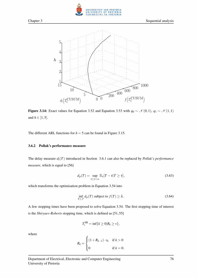
Chapter 3 Sequential analysis
0200
400600
8001000
05
10151
2
3
4
5
f(TCUSUMh
)
dl(TCUSUMh
)
h
Figure 3.14: Exact values for Equation 3.52 and Equation 3.53 with q0 ∼N (0,1), q1 ∼N (1,1)
and h ∈ [1,5].
The different ARL functions for h = 5 can be found in Figure 3.15.
3.6.2 Pollak’s performance measure
The delay measure dl(T ) introduced in Section 3.6.1 can also be replaced by Pollak’s performance
measure, which is equal to [56]
dp(T ) = sup1≤τ<∞
Eτ [T − τ|T ≥ τ], (3.63)
which transforms the optimisation problem in Equation 3.54 into
infT∈T
dp(T ) subject to f (T )≥ λ . (3.64)
A few stopping times have been proposed to solve Equation 3.54. The first stopping time of interest
is the Shiryaev-Roberts stopping time, which is defined as [51, 55]
T SRv = infk ≥ 0|Rk ≥ v,
where
Rk =
(1+Rk−1) · sk if k > 0
0 if k = 0.
Department of Electrical, Electronic and Computer EngineeringUniversity of Pretoria
76

Chapter 3 Sequential analysis
0 0.2 0.4 0.6 0.8 1 1.2 1.40
50
100
150
200
250
300
350Exact Computation
Wald’s Approximation
Siegmund’s Approximation
Simulation
-0.2θ
L(θ)
orL(θ)
orL(θ)
f(TCUSUM5
)
dl(TCUSUM5
)
Figure 3.15: The different ARL functions with q0 ∼ N (0,1), q1 ∼ N (1,1), h = 5 and θ =
[−0.2,1.4].
The value of Rk can also be calculated non-iteratively via
Rk =k
∑i=1
k
∏j=i
s j.
The Shiryaev-Roberts-Pollak stopping time is closely related to Equation 3.65. The only difference
is that R0 is not initialised with 0 but is assumed to be random with distribution equal to the quasi-
stationary distribution of Rk. Another stopping time is the deterministic Shiryaev-Roberts stopping
time. The deterministic Shiryaev-Roberts method once again considers the SR statistic R0 to be
deterministic, but not necessarily equal to zero [58]. It was shown that the Shiryaev-Roberts stopping
time and the Shiryaev-Roberts-Pollak stopping time are suboptimal solutions to Equation 3.64 [57].
The Shiryaev-Roberts-Pollak stopping time is however an asymptotically optimal (λ → ∞) solution
of Equation 3.64 in an O(1) sense [56].
3.7 CONCLUSION
Many different algorithms were investigated in this chapter, of which only CUSUM (Section 3.6.1)
and a Bayesian sequential detection (Section 3.4) variation (called time-varying maximum likelihood
classification [23]) will be used in the remaining chapters. It is important to realize that even though
Department of Electrical, Electronic and Computer EngineeringUniversity of Pretoria
77

Chapter 3 Sequential analysis
only a few of the algorithms are used directly in the remaining chapters, most of the theory in this
chapter is important and is provided to derive (or understand) the algorithms that are used in the later
chapters. The Neyman-Pearson (Section 3.1) result is critical to include in this chapter as it is the
fundamental building block on which sequential analysis rests. The SPRT (Wald’s formulation–
Section 3.3) must be included as it provides the mathematical background needed to understand
CUSUM, which is merely a repeated SPRT [59]. The SPRT algorithm also helps shed light on the
Bayesian sequential detection problem. Section 3.5 (Bayesian quickest detection) and Section 3.6.2
(the Shiryaev-Roberts stopping time and its variants) are the only two sections that can be seen as
non-critical and are included for the sake of completeness. The Bayesian quickest detection algo-
rithm was not implemented on the datasets in Section 2.8, as the change point of the datasets was not
geometrically distributed. As mentioned in Section 6.3 the Shiryaev-Roberts stopping time could still
turn out to be useful (in the remote sensing field).
Department of Electrical, Electronic and Computer EngineeringUniversity of Pretoria
78

Chapter 3 Sequential analysis
Listing 3.1: The pseudo-code for determining the OC and ASN functions via simulation.
N = 100000; %amount o f s e q u e n c e s t o g e n e r a t e f o r each t h e t a
%p a r a m e t e r d e t e r m i n i n g t h e d e n s i t y o f t h e o b s e r v a b l e s e q u e n c e
s e t t h e t a e q u a l t o an e x p e r i m e n t a l r a n g e ;
S = 0 ; %t h e sum of t h e log− l i k e l i h o o d r a t i o s
accept_H_0 = 0 ; %t h e amount o f t i m e s H_0 was a c c e p t e d
t e l l e r = 0 ; %samples r e q u i r e d b e f o r e a d e c i s i o n i s made
%dens i t y_H_0 ( z ) and . . . _H_1 ( z ) a r e t h e d e n s i t y f u n c t i o n s
%of H_0 and H_1
d e l a y = z e r o s ( 1 ,N ) ; %v e c t o r o f d e l a y s f o r each t h e t a
Q = z e r o s ( 1 , l e n g t h ( t h e t a ) ) ; %t h e OC f u n c t i o n
E_T = z e r o s ( 1 , l e n g t h ( t h e t a ) ) ; %t h e ASN f u n c t i o n
f i x h ; f i x a ; %upper and lower b o u n d a r i e s o f SPRT
f o r k = 1 : l e n g t h ( t h e t a ) %i t e r a t e t h r o u g h t h e t a
accept_H_0 = 0 ; d e l a y = z e r o s ( 1 ,N ) ;
f o r n = 1 :N %per fo rm N e x p e r i m e n t s
e x i t = f a l s e ; t e l l e r = 0 ; S = 0 ;
w h i l e ! e x i t %c o n t i n u e u n t i l e x i t b o u n d a r i e s a r e c r o s s e d
t e l l e r = t e l l e r + 1 ;
draw a z from d e n s i t y wi th p a r a m e t e r t h e t a ( k ) ;
s = l o g ( dens i t y_H_1 ( z ) / dens i t y_H_0 ( z ) ) ; S = S + s ;
i f S >= h %c r o s s e d upper boundary
d e l a y ( n ) = t e l l e r ; e x i t = t r u e ;
end%i f
i f S <= −a %c r o s s e d lower boundary
accept_H_0 = accept_H_0 + 1 ;
d e l a y ( n ) = t e l l e r ; e x i t = t r u e ;
end%i f
end%w h i l e
end%f o r
Q( k ) = accept_H_0 /N; E_T ( k ) = mean ( d e l a y ) ;
end%f o r
Department of Electrical, Electronic and Computer EngineeringUniversity of Pretoria
79

CHAPTER 4
HYPERTEMPORAL TECHNIQUES
The chapter provides the technical details of all the sequential and non-sequential hypertemporal
classification and change detection algorithms that were investigated in this thesis. The chapter is
divided into three main sections, namely simulation (Section 4.1), classification (Section 4.2) and
change detection (Section 4.3).
Simulation is the creation of synthetic data in such a way that the synthetic data accurately represent
real world data or phenomena. Simulated datasets are used for algorithm development, testing and
validation, as well as for optimising instrument specifications. Simulated data are a valuable tool
and is often used by the remote sensing community [26, 68]. Most remote sensing simulators are
constructed by using a deductive approach, which means that they rely on the biophysical laws that
govern the reflection of light [26, 27]. In Section 4.1.2, an inductive multispectral hypertemporal
reflectance simulator is proposed. In contrast to deductive simulators, an inductive simulator uses a
mathematical model that is built from the statistical properties of an existing dataset. The fact that an
inductive model is built up from the statistical properties of an existing dataset enables an inductive
model to augment datasets. The inductive simulator from Section 4.1.2 will be used to generate data
for the data-intensive CUSUM algorithm presented in Section 4.3.3. The inductive model that will
be used consists of two components, namely an SHO [3] (Section 4.1.1) to model the deterministic
underlying noise-free signal and the Ornstein-Uhlenbeck process [4] (Section 4.1.2.1) to model the
residual after the SHO has been subtracted. The two-component model will be referred to, in this
chapter, as the CSHO [2], which is discussed in detail in Section 4.1.2.2. The possibility of using the
parameters of the CSHO model as features for classification is discussed in Section 4.2.4.2.
Classification is the act of arranging or organising according to class or category. Land cover classi-

Chapter 4 Hypertemporal techniques
fication using remotely sensed data is a critical first step in large-scale environmental monitoring, re-
source management and regional planning [14]. A good review of different classification approaches
is given in [14]. As mentioned in Chapter 1 the thesis focuses on hypertemporal classifiers. The
minimum distance classifier [16], the time-varying maximum likelihood classifier [23], and the three
feature groups ιιι ,θθθ and ζζζ are discussed in Section 4.2.2, Section 4.2.3 and Section 4.2.4.2 respecti-
vely. The classification results obtained after applying these approaches to the datasets in Section 2.8
can be found in Chapter 5.
Change detection is the process of identifying differences in the state of an object or phenomenon
by observing it at different times. Essentially, it involves the ability to quantify temporal effects
using multitemporal data [69]. There have been quite a number of reviews on change detection in
the remote sensing field, namely [13, 69–73]. As mentioned in Chapter 1 the thesis also focuses on
hypertemporal change detection techniques. The band differencing algorithm [7] and the windowless
CUSUM algorithm [6] are discussed in Section 4.3.2 and Section 4.3.3 respectively. The change
detection results obtained after applying the aforementioned techniques to the datasets in Section 2.8
are presented in Chapter 5.
4.1 SIMULATION
As stated in the previous section, most remote sensing simulators are constructed by using a de-
ductive approach, which means that they employ the biophysical laws that govern the reflection of
light [26, 27]. The simulator proposed in this chapter, however uses an inductive approach. An in-
ductive approach tries to fit a mathematical model on the observed time-series directly, which is then
used to simulate realistic reflectance values. The CSHO simulator proposed in this chapter is based
on a stochastic inductive model. A stochastic inductive model tries to model the observed stochas-
tic process, not just the noise-free underlying signal. The proposed simulator is not the first such
approach used in the remote sensing literature [31]. Usually it is applied to a single time-series to
enable forecasting, as is the case in [31]. The proposed simulator supplements [31], by making the
concurrent simulation of multiple dependent time-series (multispectral) possible. On the other side of
the inductive spectrum lies the complementary noise-free inductive models [74], which are used for
noise reduction. The noise-free signals are then used to extract phenological markers. These two in-
ductive approaches do not compete against each other, since they have different aims, noise reduction
versus time-series generation.
Department of Electrical, Electronic and Computer EngineeringUniversity of Pretoria
81

Chapter 4 Hypertemporal techniques
Deductive
Inductive
Stochastic Noise-free
SingleTime-series
MultipleTime-series
Supplementary
Composition Composition
Complementary
Composition
PhenologicalMarkers
Supplementary
ForecastingBootstrapping
Other sources
Bio-physicalRay tracing
Instrument specification optimizationValidation of data processing algorithms,etc...
Figure 4.1: Functional (scientific) positioning of the proposed simulator.
The deductive simulators that were mentioned earlier use bio-physical parameters such as chlorophyll
content, which can be derived from ancillary sources (for example direct measurement). An inductive
simulator is an example of one such an ancillary source (in specific applications). For example, an
inductive simulator could be used to forecast Leaf Area Index (LAI), which is a parameter required by
the PROSPECT + Scattering by Arbitrary Inclined Leaves (PROSAIL) deductive simulator [27, 75].
Since an inductive simulator is actually a possible deductive simulator input source, they are not
directly comparable. It is important to point out that inductive simulators are supplementary tools
when used with deductive simulators, as they are not required by deductive simulators, which can
function independently from inductive simulators. Figure 4.1 illustrates the scientific positioning of
the simulator proposed in this chapter relative to existing simulators and models.
Department of Electrical, Electronic and Computer EngineeringUniversity of Pretoria
82

Chapter 4 Hypertemporal techniques
4.1.1 Noise-free inductive models
In this section, a short overview will be given of some of the different noise-free inductive models
that are currently in use. The proposed stochastic inductive simulator uses an underlying inductive
noise-free model (deterministic part) as its base. To make the simulator stochastic, a stochastic model
is added to the deterministic base, which is the primary differentiating factor between noise-free
modelling and stochastic modelling. In stochastic modelling the statistical properties of an observed
class are replicated, while deterministic modelling wants to determine the shape of the underlying
noise-free signal, and as such provides complementary functionality. The stochastic model does not
necessarily require the best possible underlying noise-free model, as long as the model used for the
residual preserves the statistical properties of the original signal.
The SHO model is an example of a noise-free inductive model [3] and is given by
Asin(2π fst +φ)+C, (4.1)
where
A,C
are the harmonic features proposed by [5, 10] and Ts =1fs
is the period of the model. Many other
models have been proposed as an improvement on the SHO model [31, 74, 76–78].
In particular, Carrão et al. [74] modelled MODIS time-series with a harmonic non-linear solution of
a chaotic attractor
C+Acos(2π fst +φ +α cos(2π fst +ζ )).
The function of each parameter used by Carrão’s model is discussed below:
• C is a linear parameter that represents the annual mean of the model.
• A is the amplitude for the sine wave that fixes the peak deviation from the annual mean of the
model.
• φ is the annual phase (produces a specific season of a given land cover class).
• α controls the non-linear strength of the model. When α = 0, the model reduces to a simple
harmonic oscillator, whereas α > 0 introduces non-symmetry (bi-annual behaviour) in the mo-
del.
Department of Electrical, Electronic and Computer EngineeringUniversity of Pretoria
83

Chapter 4 Hypertemporal techniques
• ζ is the annual nonlinear phase. This phase allows time to “slow down” and to “accelerate” in
order to reproduce asymmetries in variations (increases versus decreases).
Figure 4.2 illustrates the effect of the model parameters, as well as some of the different wave shapes
that Carrão’s model can represent.
0 5 10 15 20 25 30 35 40 45-1
-0.8
-0.6
-0.4
-0.2
0
0.2
0.4
0.6
0.8
1
(a) ∆ =− π
2 .
0 5 10 15 20 25 30 35 40 45-1
-0.8
-0.6
-0.4
-0.2
0
0.2
0.4
0.6
0.8
1
(b) ∆ = π
2 .
0 5 10 15 20 25 30 35 40 45-1
-0.8
-0.6
-0.4
-0.2
0
0.2
0.4
0.6
0.8
1
(c) ∆ = 0.
0 5 10 15 20 25 30 35 40 45-1
-0.8
-0.6
-0.4
-0.2
0
0.2
0.4
0.6
0.8
1
(d) ∆ = π .
Figure 4.2: The equation for Carrão’s model is, C+Acos(2π fst + φ +α cos(2π fst + ζ )) and ∆ =
φ − ζ . The blue line is when α = 1, while the black line is when α = 0 and the red lines are for
0 < α < 1. When the parameter α > 1 Carrão’s model will exhibit bi-annual variation. To get the
specific graphs φ = 0, which only functions as a translation parameter.
Kleynhans et al. [78] modelled NDVI time-series with a triply modulated cosine function
A(t)sin(2π fst +φ(t))+C(t).
Department of Electrical, Electronic and Computer EngineeringUniversity of Pretoria
84

Chapter 4 Hypertemporal techniques
Jönsson et al. [76] modelled vegetation index time-series using Asymmetric Gaussian (AG) func-
tions, while Zhang et al. [77] used piecewise-defined local Double Logistic (DL) functions. The AG
and DL global model functions both have the following form
y(t) =H
∑h=1
c1,h + c2,hg(t;Ah),
where H denotes the number of local model functions to use. The linear parameters c1,h and c2,h res-
pectively govern the mean and the amplitude of the local function g(t,Ah), while the meta-parameter
Ah = a1, · · · ,ar determines the shape of the local function g(t,Ah). The AG local function is equal
to
g(t,a1, · · · ,a5) =
exp[−1( t−a1
a2
)a3], if t ≥ a1
exp[−1(a1−t
a4
)a5], if t < a1.
(4.2)
In Equation 4.2, a1 determines the position of the maxima (or minima) of g, while a2 and a3 determine
the width and flatness of the right half of the function g. Similarly a4 and a5 determine the width and
flatness of the left half of the function g. The DL local function is represented by
g(t;a1, · · · ,a4) =1
1+ exp(a1−t
a2
) − 11+ exp
(a3−ta4
) ,
where a1 and a3 determine, respectively, the position of the left and right inflection points and a2 and
a4 fix the rates of change at those points. The global AG and DL functions therefore respectively
require H×7 and H×6 parameters.
Verbesselt et al. [19, 20] proposed a seasonal-trend model
C1 +C2t +k
∑j=1
A j sin(2π j fst +φ j),
where C1 is the mean of the model, C2 is the slope of the linear trend and A j and φ j are responsible
for reproducing the seasonal behaviour.
From all the inductive models discussed up to this point the SHO was selected as the deterministic
base of the proposed CSHO simulator. It is a well-known fact that the SHO model is a good first order
noise-free model of a remotely sensed time-series [3].
A short discussion follows below to justify the SHO as the underlying noise-free model for the propo-
sed simulator. In the discussion, reasons are provided for not selecting the other noise-free inductive
models (in this section). Kleynhans’s model is not a possible candidate for the deterministic base of
the proposed simulator, since it is not a parsimonious model. The stochastic model that will be used
Department of Electrical, Electronic and Computer EngineeringUniversity of Pretoria
85

Chapter 4 Hypertemporal techniques
in the end should be parsimonious so that it can also be used to extract classification features. The
seasonal-trend model is also not suitable, as the trend term of the model implies that the model should
be used with a window. The model used in the end should be parsimonious and be able to simulate
a multi-year time-series. It has been shown that Carrão’s model is better than the remaining models,
i.e. better than AG and DL, as using Carrão’s model leads to lower fitting errors [74]. Carrão’s model
can be used as a simulator by adding white noise to it. All of the models mentioned (in particular
Carrão’s model) are definitely more accurate than the SHO model over a one-year window, but are
also computationally more intensive than the Fourier transform used by the SHO.
In particular Carrão’s method uses phase unwrapping, Levenberg-Marquardt ×2 and Ordinary Least
Squares (OLS) as functional blocks for estimating the parameters of the model [79, 80]. When the
time-series becomes multi-year and there is inter-annual variation in the data, the long-term fitting-
error made by the SHO is on average far less when compared to most of the other shapes that can
be produced by Carrão’s model (the SHO is one of the shapes Carrão’s model can produce and is
obtained when α = 0). A summary of some of the shapes Carrão’s model can generate can be found
in Figure 4.2.
In other words, when the time-series becomes multi-year the SHO is actually a very good model
candidate, while the extra versatility offered by Carrão’s model becomes redundant (especially if the
first harmonic component dominates the remaining harmonic components). In the case of multi-year
time-series the increased accuracy (if any when compared to an SHO owing to the possibility of
local minima, which is relevant for Levenberg-Marquardt), benefit obtained by using Carrão’s model
no longer outweighs the computational cost of the parameter estimation technique used by Carrão’s
method (compared to the SHO). It is also important to realize that when Carrão’s model is used on
each year individually, its parsimoniousness is compromised.
4.1.2 Proposed simulator
The proposed simulator uses the CSHO model. The CSHO consists of two components, a determinis-
tic component and a stochastic component. The SHO is used for the deterministic component, while
the Ornstein-Uhlenbeck process is used for the stochastic component. The Ornstein-Uhlenbeck pro-
cess is used to model the remaining residual after the SHO is subtracted from the observed time-series.
As the SHO is very general, there will be a high degree of dependence between the observations of
the residual. The Ornstein-Uhlenbeck process can model a time-series with dependent observations
Department of Electrical, Electronic and Computer EngineeringUniversity of Pretoria
86

Chapter 4 Hypertemporal techniques
(first order), since this process is the continuous-time analogue of the discrete-time AR(1) process.
The dependence implies colouredness, which is where the name of the simulator comes from. The
Ornstein-Uhlenbeck process can be used to generate coloured noise as well as white noise [81]. The
harmonic parameters of the SHO are estimated with the Fourier transform, while the parameters of
the Ornstein-Uhlenbeck process are estimated with maximum likelihood parameter estimation. The
objective of the CSHO simulator is to simulate multispectral time-series with an inherent correlation
structure. In this thesis the simulator is used to augment datasets for data-intensive classification and
change detection algorithms (Section 4.3.3). In selective cases, statistical inductive models similar to
the CSHO have been used to forecast a single time-series [31]. The complex issue of incorporating
multispectral correlation into a simulator was however not addressed in [31]. The CSHO simulator
incorporates the average class noise correlation between the different spectral bands and reproduces
class-specific spectral behaviour (spectral dependence) by enforcing the statistical restrictions impo-
sed by different parameters (like mean and seasonal amplitude) of each spectral band in a class on
one another.
In Section 4.1.2.1 the Ornstein-Uhlenbeck process is discussed, which is followed by Section 4.1.2.2
that discusses the CSHO in detail. Section 4.1.2.3 describes the algorithm used to estimate the pa-
rameters of the CSHO. The algorithm for simulating a MODIS pixel with the CSHO is presented in
Section 4.1.2.7. The details of how the CSHO simulator enforces spectral dependence and correlation
are presented in Section 4.1.2.4, Section 4.1.2.5 and Section 4.1.2.6.
4.1.2.1 Ornstein-Uhlenbeck
The Ornstein-Uhlenbeck process is widely used in mathematical finance for the modelling of the
dynamics of interest rates and volatilities of asset prices. The Ornstein-Uhlenbeck process is the
continuous-time analogue of the discrete time AR(1) process and, when initialised with the equili-
brium distribution, is also stationary, Gaussian, Markovian and mean reverting. A stochastic process
η(t) is
• stationary if, for all t1 < t2 < · · ·< tn and h > 0, the random n-vectors (η(t1),η(t2), · · · ,η(tn))
and (η(t1 +h),η(t2 +h), · · · ,η(tn +h)) are identically distributed;
• Gaussian if, for all t1 < t2 < · · · < tn, the n-vector (η(t1),η(t2), · · · ,η(tn)) is multi-variate
normally distributed;
Department of Electrical, Electronic and Computer EngineeringUniversity of Pretoria
87

Chapter 4 Hypertemporal techniques
• Markovian if, ∀B ∈ R and for all t1 < t2 < · · · < tn, P(η(tn) ≤ B|η(t1),η(t2), · · · ,η(tn−1)) =
P(η(tn) ≤ B|η(tn−1)) (in lay man terms it means that the future is determined only by the
present and not the past).
Moreover, the Ornstein-Uhlenbeck stochastic process satisfies the following stochastic differential
equation:
dη(t) = λ (µ−η(t))dt +σdW (t), (4.3)
where λ > 0 is the rate of mean reversion, µ is the long-term mean of the stochastic process, σ > 0
is the volatility or average magnitude, per square-root time, of the random fluctuations and W (t)
is a standard Brownian motion on t ∈ [0,∞], implying that dW (t) ∼ N (0,√
dt). The solution to
Equation 4.3 is given by
η(t) = η(0)e−λ t +µ(1− e−λ t)+∫ t
0σeλ (s−t)dW (s),
where the integral on the right-hand side is an Itô integral. The equilibrium density of the Ornstein-
Uhlenbeck process is equal to N (µ, σ2
2λ). If the random fluctuations in the process are ignored, it
becomes clear that η(t) has an overall drift towards the process mean µ . The process η(t) reverts to
the mean exponentially, at a rate λ , with a magnitude in direct proportion to the distance between the
current value of η(t) and µ [82].
4.1.2.2 Coloured Simple Harmonic Oscillator
Let xc(t) = xbc(t)b∈1,··· ,7 denote a MODIS pixel at time t with assigned class label c ∈ C , where
xbc(t) denotes the bth spectral band’s reflectance at time t. The c is omitted if the class of the MODIS
pixel is unknown.
Each observed signal belonging to the same class is a sample path of a stochastic process Xbc (t).
Each MODIS class c is therefore modelled as a set of correlated (spectrally) stochastic processes
Xc(t) = Xbc (t)b∈1,··· ,7. Since Xb
c (t) is a stochastic process, an analytic expression can be assigned
(if such an expression exists) to each sample path (MODIS pixel) xbc(t;θθθ
bc) of Xb
c (t), where θθθbc is
a set of random values with a joint probability density function. It is important to realise that real
world MODIS pixels are also spatially correlated, while the proposed model assumes spatial inde-
pendence.
Department of Electrical, Electronic and Computer EngineeringUniversity of Pretoria
88

Chapter 4 Hypertemporal techniques
The proposed analytic expression for each MODIS pixel in each band (sample path) is given by
xbc(t;θθθ
bc) = sb
c(t;Abc ,φ
bc ,C
bc)+η
bc (t;µb
c ,λbc ,σ
bc ), (4.4)
where sbc(t;Ab
c ,φbc ,C
bc) is the SHO model given in Equation 4.1 with period Ts =
1fs= 45. The noise
process ηbc (t;µb
c ,λbc ,σ
bc ) is an Ornstein-Uhlenbeck process that satisfies the stochastic differential
equation given in Equation 4.3.
For each class and band, it is expected that µbc will be insignificant relative to Cb
c , as µbc = 0 if
the parameter Cbc is estimated without error. For convenience θθθ
bc will sometimes be omitted from
xbc(t;θθθ
bc).
The distribution of θθθbc is determined by the parameter set Ab
c ,φbc ,C
bc ,λ
bc ,σ
bc and it follows that
θθθ c = θθθ bcb∈1,··· ,7 = Ab
c ,φbc ,C
bc ,λ
bc ,σ
bc b∈1,··· ,7 = θ1, · · · ,θ35. The probability density function
associated with θθθ c is denoted with fc(θθθ c). When NDVI is included in the parameter set the notation
θθθ c will be used. The same convention applies for Xc(t) and xc(t). NDVI is excluded when construc-
ting the probability density function fc(θθθ c), since NDVI must be constructed from bands 1 and 2.
The notation for a MODIS pixel (plus NDVI) is represented graphically in Figure 4.3 (where x[i] is
the discrete analogue of x(t)).
45
Jan, x[1]
Dec, x[45]MODISpixel
500m
500 m
x[N ]
1 2 3 4
5 6 7 NDVI
single multispectral pixel
x5[1]
Figure 4.3: Time-series data representation for a single pixel, plus NDVI [2] © IEEE 2012.
The ensemble mean for Xc(t) is defined as
yc(t) = E [Xbc (t)]b∈1,··· ,7,NDVI, (4.5)
and is assumed to be periodic, i.e. yc(t) = yc(t +45 j), ∀ j ∈ N.
Department of Electrical, Electronic and Computer EngineeringUniversity of Pretoria
89

Chapter 4 Hypertemporal techniques
The autocorrelation of xc(t) is defined as Rc(τ) = Rbc (τ)b∈1,··· ,7,NDVI, where
Rbc (τ) =
(xbc(t)−E[xb
c(t)])(xbc(t + τ)−E[xb
c(t)])var(xb
c(t)). (4.6)
Although the spatial correlation is not fully incorporated into the CSHO model it can still be quan-
tified with the same notation. The spatial correlation of class c in band b ∈ 1, · · · ,7,NDVI can be
represented with a correlation matrix ρρρcb, with elements
ρcbm,n
=E[(xb
m,c(t)−E[xbm,c(t)])(x
bn,c(t)−E[xb
n,c(t)])]
std(xbm,c(t))std(xbn
n,c(t)),
where xbm,c(t) is the m-th pixel in a set of P MODIS pixels belonging to class c. The average spatial
correlation is then equal to
ρρρc = Eρρρc
bb∈1,··· ,7,NDVI. (4.7)
The CSHO does enforce a limited amount of spatial correlation through fc(θθθ c) (for instance the
sample paths of the CSHO pixels are reasonably in phase, have slight differences in long-term mean
and seasonal amplitude). As such CSHO pixels are less correlated (spatially) than the actual MODIS
pixels.
4.1.2.3 Parameter estimation
To estimate the harmonic parameters of Equation 4.4 the Fourier transform is used, while the noise
parameters will be estimated via maximum-likelihood parameter estimation. The Fourier transform
F of an observed MODIS pixel x(t) is defined as
X( f ) = F [xb(t)]b∈1,··· ,7,NDVI.
The subscript c is omitted here, since the class to which the MODIS pixel belongs is unknown.
For each band b the harmonic parameters Ab, φ b,Cb are estimated as follows:
Ab = 2|F [xb(t)]( fs)|
φb = arg(F [xb(t)]( fs))
Cb = |F [xb(t)](0)|.
In practice φ b is calculated by using a minimum squared error sinusoidal fit. The mean and amplitude
of the sinusoid used to calculate φ b are set to Ab and Cb respectively.
Department of Electrical, Electronic and Computer EngineeringUniversity of Pretoria
90

Chapter 4 Hypertemporal techniques
The parameters µb, λ b and σb for xb(t) are estimated by using maximum likelihood parameter esti-
mation. The first step is to calculate the residual by using
ηb(t) = xb(t)− Ab sin(2π f t + φ
b)+Cb.
Now let ηb[i] be the discrete time analogue of ηb(t), with ∆t being the time step of ηb[i], i.e. t = i∆t,
and I the total number of discrete time samples that are available of ηb(t). The log-likelihood function
of ηb[i] is given by [83]
L(µb,λ b, σb) =− I2
ln(2π)− I ln(σb)−·· ·
· · · 12(σb)2
I
∑i=1
[η
b[i]−ηb[i−1]αb−µ
b(1−αb)]2, (4.8)
where
(σb)2 = (σb)2 1− e2αb
2λ b (4.9)
and
αb = e−λ b∆t . (4.10)
By respectively setting the partial derivative of Equation 4.8 with respect to µb,λ b, σb equal to 0 and
respectively solving for µb,λ b, σb, such that µb is independent of λ b and σb, the following maximum
likelihood estimators are obtained
µb =
ηlηkk−ηkηkl
I(ηkk−ηkl)− (η2k −ηkηl)
,
λb =− 1
∆tln
ηkl− µbηk− µbηl + I(µb)2
ηkk−2µbηk + I(µb)2 ,
ˆσb =1I[ηll−2α
bηkl +(αb)2
ηkk · · ·
−2µb(1− α
b)(ηl− αbηk)+ I(µb)2(1− α
b)2],
with
ηk =I
∑i=1
ηb[i−1], ηl =
I
∑i=1
ηb[i],
ηkk =I
∑i=1
ηb[i−1]2, ηkl =
I
∑i=1
ηb[i−1]ηb[i], ηll =
I
∑i=1
ηb[i]2,
where the relation between σb and ˆσb is defined in the same way as in Equation 4.9 and αb is defined
in the same manner as in Equation 4.10. The estimated parameters can now be used as classification
features.
Department of Electrical, Electronic and Computer EngineeringUniversity of Pretoria
91

Chapter 4 Hypertemporal techniques
4.1.2.4 Parameter probability density function
All the estimated parameters (of all pixels in a specific class) are represented by the vector ΘΘΘc =
Θ1,Θ2, · · · ,Θ35, where Θi is a random variable and θi (or rather θi) is a realisation of it. Note
that NDVI is excluded from the parameter probability density function, as it is created from MODIS
land bands 1 and 2. The joint density of ΘΘΘc is assumed to be Gaussian distributed and expressed
with
fc(θθθ c) =1√
(2π)|θθθ c||ΣΣΣ|exp[− 1
2(θθθ c−µµµ)ΣΣΣ−1(θθθ c−µµµ)
]. (4.11)
In Equation 4.11, µµµ =E[ΘΘΘc] and ΣΣΣ is the covariance matrix with elements Σn,m =E[(Θn−µΘn)(Θm−µΘm)], ∀m,n ∈ 1, · · · , |θθθ c|.
4.1.2.5 Parameter and noise correlation
The parameter correlation matrix PPPcp has elements Pn,m =
E[(Θn−µΘn )(Θm−µΘm )]σΘn σΘm
, ∀m,n ∈ 1, · · · , |θθθ c|.The parameter correlation matrix PPPc
p is used to get an indication of the dependence between the model
parameters of each class and is used to model class-specific spectral behaviour.
In addition to PPPcp, the noise correlation PPPc
η is measured between the different MODIS bands. To de-
termine the noise correlation, dW b(t) from Equation 4.3 needs to be estimated, since dW b(t) induces
the random behaviour in the noise. To estimate dW b(t), ηb(t) is discretised with timesteps of length
∆t. An exact formula that holds for ∆t = 1 is [83]
ηb[i] = e−λ b
ηb[i−1]+ (1− e−λ b
)µb +σb
√(1− e−2λ b
)
2λ b ∆W b[i], (4.12)
where ∆W b[i]∼N (0,1) and is equal to ∆W b[i] =W b[i]−W b[i−1].
By making ∆W b[i] the subject of Equation 4.12, it can be used to estimate (or approximate) the
independent, normally distributed innovation terms for each timestep of each MODIS band. This, in
turn, allows the computation of the correlation matrix PPPcη of the innovation terms across the spectral
bands with Pn,m =E[(Ωn−µΩn )(Ωm−µΩm )]
σΩn σΩm, ∀m,n ∈ 1, · · · ,7, where Ωn is the random variable with
realisations ∆W n and n refers to the MODIS band.
Department of Electrical, Electronic and Computer EngineeringUniversity of Pretoria
92

Chapter 4 Hypertemporal techniques
4.1.2.6 Generating correlated innovations
Independent, correlated innovations are generated by following the approach presented in [84]. Consi-
der d independent standard (i.e. unit variance) white noise processes ∆W1, . . . ,∆W
d each of length
I, where I is the number of observations that needs to be simulated. Let furthermore a (deterministic
and constant) matrix
δδδ =
δ11 δ12 · · · δ1d
δ21 δ22 · · · δ2d...
.... . .
...
δ71 δ72 · · · δ7d
be given, and consider the seven-dimensional process ∆∆∆WWW c, defined by
∆∆∆WWW c = δδδ∆∆∆WWW , (4.13)
where
∆∆∆WWW c = [∆W 1c , · · · ,∆W 7
c ]T .
Moreover, assume that the rows of δδδ have unit length, i.e.
‖δi#‖2 = 1, i = 1, . . . ,7. (4.14)
Then each of the components ∆W 1c , · · · ,∆W 7
c separately is also a standard (i.e. unit variance) white
noise process, with instantaneous correlation given by
PPPcη = δδδδδδ
∗. (4.15)
Given a positive definite correlation matrix PPPcη , δδδ can be obtained by using Cholesky factorisation
(Section A.3) [40], such that Equation 4.14 is automatically satisfied.
4.1.2.7 Simulating a MODIS pixel
Let σσσ c = σbc b∈1,··· ,7, λλλ c = λ b
c b∈1,··· ,7, µµµc = µbc b∈1,··· ,7, CCCc = Cb
cb∈1,··· ,7, AAAc =
Abcb∈1,··· ,7, φφφ c = φ b
c b∈1,··· ,7, sc(t) = sbc(t)b∈1,··· ,7 and ηηηc(t) = η(t)b
cb∈1,··· ,7. If the
CSHO model is used to simulate a MODIS pixel which belongs to class c the following steps are
required:
Department of Electrical, Electronic and Computer EngineeringUniversity of Pretoria
93

Chapter 4 Hypertemporal techniques
1. Draw θθθ c randomly from fc(θθθ c) (assuming that fc(θθθ c) has already been constructed by using
the procedure discussed in Section 4.1.2.4).
2. Generate correlated seven-dimensional innovations ∆∆∆WWW c that are characterised by the correla-
tion matrix PPPcη (assuming that PPPc
η has already been estimated via the procedure discussed in
Section 4.1.2.5) by using the procedure discussed in Section 4.1.2.6.
3. Use σσσ c and λλλ c (from θθθ c) together with ∆∆∆WWW c and Equation 4.12 to generate ηηηc(t) under the
assumption that µµµc = 0 and ηηηc(0) = 000. The first 45 observations must be ignored, to allow
ηηηc(t) to reach a state of equilibrium.
4. Use CCCc, AAAc and φφφ c (from θθθ c) and Equation 4.1 to generate sc(t).
5. Generate xc(t) using sc(t),ηηηc(t) and Equation 4.4.
6. Generate NDVI from x1c(t) and x2
c(t).
4.2 CLASSIFICATION
As mentioned in the chapter introduction, classification is the act of arranging or organising according
to class or category. Land cover classification using remotely sensed data is a critical first step in large-
scale environmental monitoring, resource management and regional planning [14]. At this point it is
prudent to point out the subtle difference between land cover and land use. Land cover refers to the
(physical) surface cover, such as vegetation, urban infrastructure, water, bare soil etc., whereas land
use refers to the (functional) purpose that the land serves, such as agriculture, recreation, or wildlife
habitat [23].
The main focus of this section will be on land cover classification. In Section 4.2.1 a short litera-
ture review is given of land cover classification techniques, followed by the presentation of three
hypertemporal classifiers in Section 4.2.2, Section 4.2.3 and Section 4.2.4. The CSHO feature set is
discussed in Section 4.2.4.2.
Department of Electrical, Electronic and Computer EngineeringUniversity of Pretoria
94

Chapter 4 Hypertemporal techniques
4.2.1 Literature review
According to [85] there are two types of analytic approaches for creating land cover maps, namely
photointerpretation and machine analysis. Photointerpretation relies on a human analyst to interpret
an enhanced image. Machine analysis on the other hand, uses statistical or numerical algorithms to
perform the labelling of multispectral datasets. A good review of different machine analysis tech-
niques (henceforth described only as classification techniques) is available in [14]. According to [14],
remote sensing classification approaches can be grouped using a taxonomy. The proposed taxonomy
in [14] can be found in Figure 4.4. A short description of each category found in Figure 4.4 is given
in [14, 23]. In [14], the classification elements are used as the primary attribute for grouping clas-
sification techniques together. In this section the classification of elements will also be used as the
primary attribute for grouping classification techniques together. The different classification elements
parametric non-parametric
data representation
hard soft (fuzzy)
classifier output
supervised unsupervised
use of training samples
per-pixel
per-field object-oriented
subpixel
classification elements
contextual-based knowledge-based
Figure 4.4: A taxonomy of fixed sample size land cover classification techniques (from [23]).
and some of the most popular algorithms used by each type of element are discussed in the following
list:
1. In per-pixel classification, each pixel is classified as belonging to a specific land cover
class. Per-pixel classification clearly assumes homogeneous pixels, which becomes unrea-
listic when the spatial resolution is decreased [23]. Per-pixel classifiers can be parametric
or non-parametric. Maximum likelihood classification is probably the most commonly used
per-pixel parametric classification approach and is presented clearly in [85]. The most fre-
quently used non-parametric per-pixel classifiers are Artificial Neural Networks (ANNs) [86],
decision trees [87,88] and SVMs [89–91]. There are some remaining advanced per-pixel-based
classification algorithms worth mentioning, which include: the spectral angle classifier [92],
Independent Component Analysis (ICA) [93, 94], a model-based approach [95, 96] and several
nearest neighbour approaches [97–99].
Department of Electrical, Electronic and Computer EngineeringUniversity of Pretoria
95

Chapter 4 Hypertemporal techniques
2. Subpixel techniques are especially used with medium or coarse resolution remote sensing data,
since heterogeneous pixels are quite common at those spatial resolutions. Typically subpixel
classification is done with either fuzzy sets [100,101] or Spectral Mixture Analysis (SMA) [102–
104]. Other prominent approaches to subpixel classification include ANNs [105], Dempster-
Shafer theory, certainty factors [106] and a maximum likelihood approach [107].
3. One way to to handle pixel heterogeneity is to employ per-field classification. In per-field clas-
sification pixels are no longer evaluated individually, but in “fields” consisting of the same land
cover type, such that the noise can be averaged out over larger areas, implying that the fields
are more homogeneous than the pixels that make up the fields (see for example [108, 109]).
Object-oriented classification is similar to per-field-based classification. The main difference is
that object-oriented methods use only raster data, whereas per-field approaches use vector and
raster data. The reference list [110–112], provides additional information on object-oriented
classification. A frequently used object-oriented approach is eCognition, which is described in
(among others) [113].
4. Contextual-based approaches to land cover classification take the spatial distribution of pixels
into account in an attempt to minimise the effects of intra-class variations [114]. In [115] a
selection of early ad hoc contextually based classifiers are compared. More recently it has been
shown that the Markov and Gibbs random fields are effective approaches that can use spatial
information [116, 117]. Markov and Gibbs random fields were introduced to image processing
by the seminal paper [118]. There are also spectral-contextual classifiers of which [119] is a
good example.
5. Knowledge-based methods use ancillary data sources (such as a digital elevation map, a soil
map, housing, etc.) on top of the contextual information that is available for a region to perform
classification (see [120] for an example).
4.2.1.1 Dimensionality reduction
The large amount of training data that hyperspectral data provide needs to be reduced, as classifiers
that use large training datasets become impractical very quickly [23]. An effective way of reducing
training datasets is to use dimensionality reduction, which is closely related to feature extraction.
Dimensionality reduction algorithms have to be able to select the most prevailing elements from a
Department of Electrical, Electronic and Computer EngineeringUniversity of Pretoria
96

Chapter 4 Hypertemporal techniques
dataset, while skipping the unimportant elements. Several approaches to dimensionality reduction
exist, including Principal Component Analysis (PCA), minimum noise fraction transform, discrimi-
nant analysis [121–123], decision boundary feature extraction [124], Gaussian mixture model feature
extraction [95], wavelet transform [125] and SMA [126].
4.2.1.2 Hypertemporal classification
Most of the classification techniques discussed in the literature review up to now have been single-
date classifiers. It has been shown that multitemporal and hypertemporal classification is more re-
liable than single-date classification [15, 127, 128], since single-date reflectance values between dif-
ferent classes may be unseparable due to the fact that land-cover classes could have similar spectral
characteristics during certain times of the year [15]. A second reason that motivates hypertemporal
classification is that most of the earth (landmass) is covered by vegetation. Vegetation species have
unique phenologies, which make remote classification possible [39]. The most prominent hypertem-
poral classification techniques in literature are PCA [17,129,130], phenological metrics [18,131,132],
Fourier analysis [5, 133–136], wavelet analysis [137], minimum distance classification [16, 23] and
time-varying maximum likelihood classification [23].
The chapter focuses on hypertemporal classification techniques. In particular it revolves around the
parameters of the CSHO. The parameters of the CSHO will be used as features that will be fed into
an SVM classifier. The proposed technique extends the approach in [5], which is based on Fourier
features. In [5], it is shown that efficient separability can in fact be achieved when using only the
mean and seasonal harmonic components. The Ornstein-Uhlenbeck process, which is a component
of the CSHO, summarises the less important Fourier features that by themselves do not contribute
significantly to classification up with two average model parameters that could possibly contribute
significantly to classification accuracy. The SVM classifier with CSHO features is compared to the
minimum distance classifier [16], the time-varying model classifier [23] and SVMs fed with temporal
and harmonic features in Section 5.3.
4.2.2 Minimum distance classifier
The minimum distance classifier classifies the observed signal x(t) as class c by choosing the class
with the lowest model error [16, 23]. Where the model error for each class c is defined as the accu-
mulated euclidean distance between the observed signal x(t) and the signal model (yearly ensemble
Department of Electrical, Electronic and Computer EngineeringUniversity of Pretoria
97
Chapter 4 Hypertemporal techniques
mean) yc(t), mathematically it can be written as, find a c such that the following optimisation problem
is minimised:
infc∈C
∫ I
0‖x(t)− yc(t)‖2 dt.
Any subset of x(t) and yc(t) can be used for classification, as long as both subsets are constructed
from the same spectral bands. The euclidean differences are normalised with the difference between
the maximum and minimum observed value in each band.
4.2.3 Time-varying maximum likelihood classifier
The time-varying maximum likelihood classifier uses the time-varying model [23]. The background
theory used in this section was discussed in detail in Section 3.4. The time-varying model is a dis-
crete model and Xc(t) therefore needs to be discretised. Let the discretised form of Xc(t) be denoted
by Xc[k]k=1,2,···. The time-varying model is equivalent to the first order statistical description
of Xc[k]k=1,2,···. Usually the phrase “first order statistical description” is only associated with
a single stochastic process, but here the first order statistical description is connected with a set of
stochastic processes. The first order statistical description of Xc[k]k=1,2,··· is equal to the set of
probability density functions at each time step k, qckk=1,2···. If it is assumed that the MODIS
data contain no inter-annual variation, in other words it is assumed that the MODIS time-series is
periodic (45 observations in a year), then it is true that qck = qc
k+45n, n = 1,2, · · ·. Note that qck is
an eighth-dimensional density and that the density at k can also be constructed for a smaller number
of bands. When only a subset of the bands is used the notation qc,bk is used, where b can be any
subset of 1, · · · ,7,NDVI. The same rule applies for Xbc (t) and xb
c (t). Assume now that the class
label c is equal to either a v ≡ 0 or a s ≡ 1 if the observed MODIS pixel belongs to either the ve-
getation or settlement class. Any unlabelled MODIS pixel xb[k]k∈N obeys one of two statistical
hypotheses:
H0 : xb[k]∼ Q0,bk , k = 1,2, · · ·
versus
H1 : xb[k]∼ Q1,bk , k = 1,2, · · · ;
where for each time step k, Q0,bk and Q1,b
k are two |b|-dimensional probability distributions with
associated densities q0,bk and q1,b
k , respectively. Further assume that hypothesis H1 occurs with prior
probability π and H0 with prior probability 1−π .
Department of Electrical, Electronic and Computer EngineeringUniversity of Pretoria
98

Chapter 4 Hypertemporal techniques
Now define the posterior sequence to be
ππk =
ππk−1q1,b
k (xb[k])
ππk−1q1,b
k (xb[k])+(1−ππk−1)q
0,bk (xb[k])
, k = 1,2, · · · ,
where ππ0 = π . The maximum likelihood classification of the time-varying classification task is then
given by
δk =
0, if ππk ≤ 0.5
1, if ππk > 0.5.
If thresholds are introduced to the time-varying maximum likelihood classifier then the time-varying
maximum likelihood classifier becomes sequential in nature. Let πU,πL be those thresholds. If ππk
crosses πU,πL a decision can be made. The decision rule now becomes
δk =
0, if ππk ≤ πL
1, if ππk > πU.
It can easily be shown (see Section 3.4.2 for more details) that the sequential time-varying maximum
likelihood classifier is equivalent to the time-varying SPRT (in terms of classification accuracy and
delay), where the time-varying SPRT is obtained by casting the classification problem presented in
this section into the likelihood domain. Currently the classification problem is solved using a posterior
sequence.
4.2.4 Support Vector Machine
An SVM works by creating a hyperplane or set of hyperplanes in a high or infinite dimensional
space, and as such can be used for classification, regression, or to perform other similar functions
[1, 138, 139]. An SVM works on the principle of finding a hyperplane, such that the hyperplane has
the furthest distance from the training data of any class (which is known as the functional margin).
The training data for the classifier are a set of n points of the form
D = (r(i),ψ(i)|r(i) ∈ Rp,ψ(i) ∈ −1,1 (4.16)
where ψ(i) is a label denoting class membership, and r(i) is a p-dimensional real feature vector. If the
data are linearly separable, a maximum-margin hyperplane is calculated to divide the data into points
belonging to the class with label −1 or 1 perfectly. The maximum-margin hyperplane is represented
by the following
wT · r+b = 0, (4.17)
Department of Electrical, Electronic and Computer EngineeringUniversity of Pretoria
99

Chapter 4 Hypertemporal techniques
Margin
w
Origin
b
‖w‖
H2
H1
Figure 4.5: Example of a maximum-margin hyperplane of a linear SVM (from [23]).
where vector w is perpendicular to hyperplane, Equation 4.17, and b||w|| is the offset of hyperplane,
Equation 4.17, from the origin in the direction of w. The maximum-margin hyperplane is calculated
by choosing w and b to maximise the distance between the hyperplanes wT · x + b = −1 (which
corresponds to hyperplane H1 in Figure 4.5) and wT · x+ b = 1 (which corresponds to hyperplane
H2 in Figure 4.5). These two hyperplanes are as far a part as possible although they still correctly
classify each training data point. The problem of maximising the distance between the hyperplanes
wT ·x+b =−1 and wT ·x+b = 1 reduces to the following optimisation problem:
minw,b
12||w||2
s.t. ψi(wT · r+b)≥ 1, i = 1, · · · ,n. (4.18)
Equation 4.18 is known as the primal problem. The optimisation problem is actually solved by using
the so-called dual problem, which is the Lagrangian reformulation of the primal problem. There
are mainly two reasons for rather solving the dual problem, namely the constraints of Equation 4.18
are supplanted by constraints of the Lagrange multipliers themselves, which are much easier to deal
with, and in the dual problem inner products are used in both the training and testing algorithms,
which makes it possible to effortlessly generalise to non-linear SVMs [23]. Readers interested in
the dual problem are referred to [139], which is a comprehensive tutorial on SVMs. To extend the
Department of Electrical, Electronic and Computer EngineeringUniversity of Pretoria
100

Chapter 4 Hypertemporal techniques
approach to non-separable datasets the optimisation problem is reformulated to obtain:
minw,b
12||w||2 +C
n
∑i=1
ξi
s.t. ψi(wT · r+b)≥ 1−ξi, i = 1, · · · ,n
ξi ≥ 0, i = 1, · · · ,n.
The method entails, introducing slack variables, ξi, which measure the degree of misclassification
of ri. The parameter C controls the relative weighting between the slack variables and the goal
minw,b12 ||w||2.
An SVM was chosen as classification technique since SVMs, unlike neural networks, are robust to the
over-fitting problem (increased spectral view increases feature set sizes). The first documented use
of SVMs in remote sensing was in [140]. A good review of the application of SVMs in the remote
sensing field can be found in [91], of which [89, 141–143] are worth singling out. It is also worth
mentioning [15, 144–148], as these works applied SVMs to MODIS data.
4.2.4.1 Example
Consider the following linearly separable binary classification problem:
ρρρ = [w1,w2,b]T ,w = [w1,w2]T .
r = [r1,r2]T .
The aim is to find a hyperplane wT r+ b = 0 that separates the binary classes perfectly, while the
margin between wT r + b = −1 and wT r + b = 1 is also maximised. The following six training
examples are given,
r(1) = [1,1]T = (1,1),
r(2) = [1,2]T = (1,2),
r(3) = [2,1]T = (2,1),
r(4) = [3,3]T = (3,3),
r(5) = [2,4]T = (2,4),
r(6) = [4,5]T = (4,5).
With classification given by the label ψ(i) ∈ −1,+1 for each training example,
ψψψ = [−1,−1,−1,1,1,1].
Department of Electrical, Electronic and Computer EngineeringUniversity of Pretoria
101

Chapter 4 Hypertemporal techniques
The given binary classification problem is represented graphically in Figure 4.6. The hyperplane
0 0.5 1 1.5 2 2.5 3 3.5 4 4.50
1
2
3
4
5
w · x− b = 0
w · x− b = −1
w · x− b = 1
r1
r 2 w
Figure 4.6: An example of an SVM classification problem.
wT r + b = 0 for this example can be found by solving the following primal minimisation pro-
blem.
Minimize f (ρρρ) =12‖w‖2 =
12
wT w, (4.19)
such that g1(ρρρ) = w1 +w2 +b+1≤ 0,
g2(ρρρ) = w1 +2w2 +b+1≤ 0,
g3(ρρρ) = 2w1 +w2 +b+1≤ 0,
g4(ρρρ) =−2w1−4w2−b+1≤ 0,
g5(ρρρ) =−3w1−3w2−b+1≤ 0,
g6(ρρρ) =−4w1−5w2−b+1≤ 0,
Department of Electrical, Electronic and Computer EngineeringUniversity of Pretoria
102

Chapter 4 Hypertemporal techniques
which can be transformed to have only equality constraints by introducing the auxiliary variables, κ j.
After introducing the auxiliary variables Equation 4.19 reduces to:
minimise f (ρρρ) =12‖w‖2 (4.20)
such that h1(ρρρ) = w1 +w2 +b+1+κ21 = 0,
h2(ρρρ) = w1 +2w2 +b+1+κ22 = 0,
h3(ρρρ) = 2w1 +w2 +b+1+κ23 = 0,
h4(ρρρ) =−2w1−4w2−b+1+κ24 = 0,
h5(ρρρ) =−3w1−3w2−b+1+κ25 = 0,
h6(ρρρ) =−4w1−5w2−b+1+κ26 = 0.
The constraints in Equation 4.19 follow from the requirement that
ψ(i)(
wT r(i)+b)≥ 1, ∀i = 1, . . . ,6. (4.21)
Now the Lagrange function (Section A.4) [40] of Equation 4.20 can easily be constructed, which is
equal to
L (ρρρ,κκκ,λλλ ) = f (ρρρ)+6
∑j=1
λ j(g j(ρρρ)+κ2j )
with λλλ being the Lagrange multiplier. The Lagrange function can be used for solving Equation 4.19
by setting each of its partial derivatives to zero and solving the set of equations formed. Taking the
partial derivative of the Lagrange function with respect to each of its variables yields the following
Department of Electrical, Electronic and Computer EngineeringUniversity of Pretoria
103

Chapter 4 Hypertemporal techniques
set of equations:
∂L
∂w1= w1 +λ1 +λ2 +λ3−2λ4−3λ5−4λ6,
∂L
∂w2= w2 +λ1 +2λ2 +λ3−4λ4−3λ5−5λ6,
∂L
∂b= λ1 +λ2 +λ3−λ4−λ5−λ6,
∂L
∂κ j= 2λ jκ j ∀i 1 . . .6,
∂L
∂λ1= w1 +w2 +b+1+κ
21 ,
∂L
∂λ2= w1 +2w2 +b+1+κ
22 ,
∂L
∂λ3= 2w1 +w2 +b+1+κ
23 ,
∂L
∂λ4= −2w1−4w2−b+1+κ
24 ,
∂L
∂λ5= −3w1−3w2−b+1+κ
25 ,
∂L
∂λ6= −4w1−5w2−b+1+κ
26 .
Setting the above equations to zero and solving produces the following result:
w∗1
w∗2
b∗
κ∗1
κ∗2
κ∗3
κ∗4
κ∗5
κ∗6
λ ∗1
λ ∗2
λ ∗3
λ ∗4
λ ∗5
λ ∗6
=
2/3
2/3
−3
0.8165≈ 49/60
0
0
0
0√
2
0
0
4/9
−2/9
2/3
0
(4.22)
Department of Electrical, Electronic and Computer EngineeringUniversity of Pretoria
104

Chapter 4 Hypertemporal techniques
The first three solutions of Equation 4.22 are also the solution of Equation 4.19, ρρρ∗ = [2/3,2/3,−3],
which completely describes the hyperplane wT r+b = 0. The hyperplane can be rewritten in terms of
r1 and r2.
wT r+b = w1r1 +w2r2 +b
= 2/3r1 +2/3r2−3
= 0
leading to the normal straight line r2 =−r1 +4.5.
4.2.4.2 Proposed features
Three main sets of SVM features will be presented. The first feature set consists of the harmonic
components of Equation 4.4 and is denoted by
ιιι = Cb,Abb∈1,··· ,NDVI. (4.23)
Any spectral subset of ιιι can also be selected, and is denoted by ιιιb, where b is any subset of
1, · · · ,NDVI. Fourier (or spectral) analysis, on NDVI time-series in particular, has been used ex-
tensively for land cover classification (see for example [5, 78, 134, 149]), and it has been shown that
reliable class separation can be achieved even when considering only the mean and seasonal spectral
components [5, 78], i.e. Equation 4.23.
The second feature set consists of noise-harmonic features, i.e. consists of all the parameters in
Equation 4.4 and is represented mathematically with
θθθ = Cb,Ab,φ b,λ b,σbb∈1,··· ,NDVI.
As in the case of ιιι , a spectral subset of θθθ is denoted by θθθb. The benefit of θθθ when compared to
ιιι is that θθθ also includes the parameters of the Ornstein-Uhlenbeck process, which are λλλ and σσσ .
The Ornstein-Uhlenbeck process summarises the less important Fourier features that by themselves
do not contribute significantly to classification up with two model parameters that could contribute
significantly to classification accuracy.
The third feature set is composed of temporal features. Selecting temporal features for classification
purposes is a well-known approach [15]. If the most relevant reflectance values of a MODIS pixel
x(t) are to be chosen, then those reflectance values from x(t) where the annual ensemble mean of two
Department of Electrical, Electronic and Computer EngineeringUniversity of Pretoria
105

Chapter 4 Hypertemporal techniques
different classes are at a maximum distance from each other need to be selected. Mathematically it
can be expressed as follows: a τ should be selected such that the following optimisation problem is
maximised.
supτ∈1,··· ,45
‖yc1(τ)− yc2(τ)‖2,
where y represents the annual ensemble mean. The solution τ can be extended to a sequence τττ;
since the annual ensemble mean is periodic, a maximum can be attained more than once during
the observation period I. Now the actual reflectance values from the observed MODIS pixel are
selected,
ζζζ = x(τττ) = xb(τττ)b∈1,··· ,7,NDVI.
A smaller ζζζb can be constructed by using subsets of yc1(t), yc2(t) and x(t), as long as the subsets are
constructed by using the same spectral bands. Now, ιιι , θθθ or ζζζ can be substituted into rrr(i) (see Equa-
tion 4.16). As mentioned in Chapter 1, the shorthand notation ιιι ,θθθ and ζζζ will be used to respectively
refer to each feature set group, namely harmonic features, noise-harmonic features and temporal fea-
tures.
4.3 CHANGE DETECTION
As stated in the chapter introduction, change detection is the process of identifying differences in
the state of an object or phenomenon by observing it at different times. Essentially, it involves the
ability to quantify temporal effects using multitemporal data [69]. Usually land cover changes are
categorised into land cover conversion and land cover modification [71]. Land cover conversion
is described in [71] as “complete replacement of one cover type by another”, whereas land cover
modification is described as “more subtle changes that affect the character of land cover without
changing its overall classification”.
In Section 4.3.1 a short literature review is given of land cover change detection techniques, fol-
lowed by the presentation of two hypertemporal change detection techniques in Sections 4.3.2 and
4.3.3.
4.3.1 Literature review
There have been quite a number of reviews on change detection in the remote sensing field, na-
mely [13, 69–73, 150]. The review written by Singh [69] in 1989 laid much of the foundation needed
Department of Electrical, Electronic and Computer EngineeringUniversity of Pretoria
106

Chapter 4 Hypertemporal techniques
to categorize remote sensing change detection approaches effectively [151]. The following main ca-
tegories were proposed by Singh, namely univariate image differencing, image regression, image
ratioing, vegetation index differencing, PCA, post-classification comparison, direct multi-date com-
parison and Change Vector Analysis (CVA). Later Lu et al. [13] improved on the categories proposed
by Singh (more organised) [151]. The categories proposed by Lu et al. are briefly discussed be-
low:
• Algebra – this category includes the methods that depend on a change metric, which is subse-
quently compared to a threshold value in order to declare a change or not. The change metric
can be computed in a variety of ways, namely image differencing [152–155], image regres-
sion [156], image rationing [157], vegetation index differencing [158] and CVA [159].
• Transformation – this category comprises methods that reduce data dimensionality. Some of
the possible approaches to reducing data redundancy are PCA [160], Kauth-Thomas [161],
Gramm-Schmidt [161] and the Chi-square transformation [162].
• Classification – post-classification comparison [163], Expectation Maximization [164,165] and
ANN [166] are some of the constituent techniques that make up the classification category. The
methods in this category use classified images and require a large amount of training data.
• Advanced models – this category includes, among others, the Li-Strahler reflectance mo-
del [167], SMA [102], and the biophysical parameter estimation model [168, 169]. The funda-
mental idea behind the methods in this category is that the reflectance values are converted to
biophysical parameters, which are more interpretable than the original raw reflectance values.
• Geographic Information System (GIS) – the integrated GIS and remote sensing method [170]
and the standard GIS approach [171] are some of the algorithms that fall into this category.
• Visual interpretation – visual interpretation requires manual interpretation of remote sensing
images at different times followed by on-screen digitation of change polygons [172].
• Other methods – many categories have now been suggested to group the different change de-
tection techniques together. There are however some techniques that do not fall into any of
the above categories, namely measures of spatial dependence [173], knowledge-based vision
systems [174], change curves [175], generalised linear models [176], the curve theorem-based
Department of Electrical, Electronic and Computer EngineeringUniversity of Pretoria
107

Chapter 4 Hypertemporal techniques
approach [177], structure based approach [178] and spatial statistics-based approach [179].
Most of the categories proposed by Lu et al. consist of methods that are multitemporal, which nor-
mally require only two images as input. There are however some reviews that explicitly discuss an
additional category called hypertemporal change detection techniques or temporal trajectory analy-
sis [71, 73]. The other categories proposed by [71, 73], will not be adopted, as the multitemporal
techniques are grouped sufficiently using the categories proposed by [13]. All the methods that are
applied to hypertemporal time-series fall into this additional category.
4.3.1.1 Hypertemporal techniques
When considering multi-date change detection, a serious consideration is the selection of optimal
image dates. This problem can be circumvented by considering a hypertemporal time-series [10].
The last decade has seen a dramatic increase in the number of papers published in the field of hy-
pertemporal change detection (remote sensing) [7, 12, 19–21, 28, 151, 180–193], some of which are
discussed briefly below.
Temporal change metrics are used in [180] to detect land cover changes. The temporal change metrics
are computed by computing the annual difference (year2-year1) of the annual maximum, annual mini-
mum and annual range. In addition to the above metrics, the magnitude of the multitemporal change
vector is also calculated. These metrics are then compared with a threshold to determine whether
a change has occurred or not. In [7], a change is detected by identifying abnormal pixel behaviour.
These pixels are identified by selecting pixels that show a significant deviation in the annual difference
of the yearly total NDVI relative to other pixels from the same class and study area. In [184, 185] a
disturbance index is computed to detect large-scale ecosystem disturbances. The disturbance index
is calculated on an annual basis by dividing two ratios. The top ratio is calculated by dividing the
annual maximum land surface temperature LSTmax with the annual maximum Enhanced Vegetation
Index (EVI) EVImax, while the bottom ratio is calculated by dividing the multi-year mean of LSTmax
with the multi-year mean of EVImax. The disturbance index is then compared with a predetermined
threshold to determine whether a change flag is required. The departure from a model algorithm, the
recursive merging algorithm and the yearly delta algorithm are some of the multitemporal techniques
proposed in [28, 187]. A generic change detection approach is proposed in [19, 20] for NDVI time-
series by detecting and characterising Breaks for Additive Seasonal and Trend (BFAST). Lastly, it
is worth mentioning the sliding window approach documented in [21], the autocorrelation approach
Department of Electrical, Electronic and Computer EngineeringUniversity of Pretoria
108

Chapter 4 Hypertemporal techniques
proposed in [189, 190] and the Kalman filter approach presented in [191].
Most of the remote sensing hypertemporal change detection algorithms in the literature use some form
of windowing, in other words only recent data are used to detect change. In contrast the hypertemporal
change detection algorithm proposed in Section 4.3.3 (Page’s original CUSUM algorithm [6]) is
windowless, consequently no step is required to determine the window length.
There are several metrics by which a change detection algorithm should be evaluated. An obvious
one is detection delay, which is the time taken for the change detection algorithm to declare that a
change has occurred, given that a change in the data actually occurred. Then there is the question
of how likely it is for the algorithm to declare that a change has occurred, given that the change in
the data did in fact occur, a metric that is referred to as either probability of detection or the True
Positive Rate (TP). There are more metrics that need to be considered. For example, there is the
possibility that the algorithm will declare change, even though no change has occurred in the data,
which can be referred to as either the probability of false detection (alarm) or the False Positive
Rate (FP). As this chapter is presented in a statistical framework, the detection theory terms TP and
FP will not be adopted. Then there is the question of how to eliminate the need for a windowing
mechanism, in the sense that the proposed algorithm is on-line or sequential, i.e. it uses all the past
data. This is possible when the algorithm has the property that it only starts behaving differently
when an actual change has occurred. However, it is not common for the above four change detection
criteria to be considered simultaneously in a remote sensing change detection context, and in that
respect the proposed algorithm is novel, since it can sequentially detect change (vegetation pixels
that are changed into settlement pixels) as accurately and quickly as possible, while staying below a
certain probability of false alarm.
The proposed change detection algorithm (Section 4.3.3) uses Page’s original CUSUM algorithm in
order to process samples sequentially [6]. Windowed versions of the CUSUM algorithm have been
used with MODIS in the past, typically in a bootstrapping [194] or in an in-control process mean
context [28, 29]. The problem with using only recent data, which was extracted using a window, is
that the average pixel behaviour might not be captured if the window is not long enough. The next
example highlights the main drawback of using a window.
In Figure 4.7, the time-series of a vegetation pixel in Gauteng (that did not change from land cover
type) over 8 years and its filtered output (which could be considered as the in-control process mean)
Department of Electrical, Electronic and Computer EngineeringUniversity of Pretoria
109

Chapter 4 Hypertemporal techniques
is presented in Figure 4.7. Clearly to select a proper history period is quite difficult in the case of
2001 2002 2003 2004 2005 2006 2007 2008 20095
7
9
11
13
15
FilteredData
%R
eflec
tan
ce
Figure 4.7: Temporal behaviour of a vegetation pixel (Gauteng) in MODIS band 1, and its filtered
output (first 10 FFT components).
Figure 4.7. An improper estimated in-control process mean (due to a bad history period) will lead
to wrongly estimated residuals (larger than they should be). Larger residuals cause an unnecessary
amount of false alarms. Which is why CUSUM performs so badly for the approach presented in
[28, 187].
CUSUM can be implemented without using a window, because in Page’s original form the CUSUM
statistic is derived from log-likelihood ratios, which can be obtained from densities estimated at every
time-step of the year. The densities at each time-step thus circumvents intra-annual variation. The
densities are constructed by using the CSHO, which can replicate average pixel behaviour which
implies that the effect of inter-annual variation is also minimised (see Section 5.2.4.4) [2, 30, 32].
The CUSUM change detection algorithm is compared with the popular band differencing approach
(Section 4.3.2) in Section 5.4 [7, 10, 28].
4.3.2 Lunetta et al.’s scheme
Let xp[k] = xbp[k]b∈1,··· ,7,NDVI be the p-th discrete MODIS pixel in a set of P unlabelled pixels. The
c subscript is omitted as the class of the pixel is unknown. The change detection scheme proposed by
Lunetta et al. can be implemented with the following steps [28]:
1. The signal xp[k] is first filtered, by keeping only the first ν components of an I point Fast Fourier
Transform (FFT), where I is equal to the temporal dimension of xp[k].
Department of Electrical, Electronic and Computer EngineeringUniversity of Pretoria
110

Chapter 4 Hypertemporal techniques
2. For each pixel p compute the annual sum for each year of data (of which there are Y years). Let
ap1, · · · ,apY correspond to this list of annual sums, where ap1 = ∑45k=1 xb
p[k]b∈1,··· ,7,NDVI,
etc.
3. For each pixel p compute the difference between consecutive annual sums, i.e., ap2 −ap1,ap3 − ap2,apY − apY−1, where ap2 − ap1 = ab
p2 − abp1b∈1,··· ,7,NDVI, etc. Let dp j =
ap j+1−ap j.
4. For each pixel p compute the z − score
zp j =dp j−µµµ j
σσσ j
for each of the Y − 1 va-
lues in dp1,dp2, · · · ,dpY−1. This is done for each dp j by subtracting the mean (µµµ j =
Ed1 j,d2 j, · · · ,dP j = Edb1 j,d
b2 j, · · · ,db
P jb∈1,··· ,7,NDVI) and dividing by the standard de-
viation (σσσ j =√
E(d1 j)2,(d2 j)2, · · · ,(dP j)2− (µµµ j)2, where (d1 j)
2 = (db1 j)
2b∈1,··· ,7,NDVI,
etc.). Note that the mean and the standard deviation are computed across space. Let
zp1,zp2, · · · ,zpY−1 correspond to this list of z-scores.
5. For each pixel p compute the change score cp = max|zbp1|, |zb
p2|, · · · , |zbpY−1|b∈1,··· ,7,NDVI.
A change or no change decision can now be reached in every band by comparing cp with the
eight-dimensional threshold hl . If cp > hl a change is declared.
4.3.3 Cumulative Sum
The CUSUM algorithm is discussed in detail in Section 3.6. To apply the CUSUM algorithm to
MODIS time-series it needs to be modified slightly. The modified CUSUM algorithm that is presented
in this section is also applied to the first order statistical description of Xc[k]k=1,2,···, which was
introduced in Section 4.2.3. There is however a slight difference; the CUSUM algorithm will only
be applied to individual bands, so that a fair comparison with Lunetta et al.’s scheme is possible (no
multispectral densities are considered). The modified CUSUM stopping time is given by
TCUSUMh = infk≥ 0|gk ≥ hc,
where
gk =
(gb
k−1 + sbk)
+b∈1,··· ,7,NDVI k 6= 0
y ∈ R+8 k = 0
and
sbk = ln
q1,bk (xb(k))
q0,bk (xb(k))
. (4.24)
Department of Electrical, Electronic and Computer EngineeringUniversity of Pretoria
111

Chapter 4 Hypertemporal techniques
Under normal CUSUM operating conditions y= 0= 0,0,0,0,0,0,0,0. As soon as gbk ≥ hb
c a change
can be declared in band b. It is important to realise that the optimality of CUSUM (and the optimality
of the sequential time-varying classifier) can no longer be guaranteed because of the following list of
shortcomings:
1. The identically distributed assumption is violated by Equation 4.24.
2. The MODIS time-series does not consist of independent observations.
3. The densities q0,bk and q1,b
k are estimated and not known beforehand.
4. In reality the MODIS pixels are spatially correlated.
The densities at each time-step can be estimated from ground truth data or via a trained CSHO simu-
lator. Furthermore, it should also be obvious to the reader that the CUSUM algorithm presented here
is nothing more than a repeated time-varying SPRT (see Section 4.3.3) [59].
4.4 CONCLUSION
The chapter presented the details of all the sequential and non-sequential hypertemporal classification
and change detection algorithms that were investigated in this thesis. The chapter was divided into
three main sections, namely simulation (Section 4.1), classification (Section 4.2) and change detec-
tion (Section 4.3). The chapter primarily dealt with a new stochastic inductive model, the CSHO
(Section 4.1.2.2) and the model’s possible application in simulation (Section 4.1.2.2), classification
(Section 4.2.4.2) and change detection (Section 4.3.3). The experimental results of all the algorithms
presented in this chapter will be given in Chapter 5. Note that the time-varying maximum likelihood
classifier (with thresholds) in Section 4.2.3 and the CUSUM algorithm in Section 4.3.3 are sequential
approaches.
Department of Electrical, Electronic and Computer EngineeringUniversity of Pretoria
112

CHAPTER 5
RESULTS
The chapter starts with preliminary data analysis results obtained from the datasets introduced in
Section 2.8. These results can be used to predict the performance of the different classification and
change detection approaches. In Section 5.2 the inductive simulator discussed in Section 4.1.2 is
validated. The final sections of the chapter give the classification and change detection accuracies
and rankings of the different sequential and non-sequential hypertemporal classification and change
detection algorithms discussed in Chapter 4.
5.1 PRELIMINARY DATA ANALYSIS: GAUTENG AND LIMPOPO
In this section a preliminary investigation of the datasets introduced in Chapter 2 is performed. The
knowledge gained from the preliminary analysis is used to explain the classification and change de-
tection results of Section 5.3 and Section 5.4. The data analysis is conducted under the following
headings: yearly ensemble mean (Section 5.1.1), temporal Hellinger distance (Section 5.1.2), CSHO
parameters (Section 5.1.3), noise correlation (Section 5.1.4) and spatial correlation (Section 5.1.5).
An important data manipulation technique used in the remainder of the section is temporal grouping
of multispectral observations and is expressed in mathematical notation below.
Recall from Chapter 4 that each MODIS pixel (which is denoted here explicitly by xc) has eight asso-
ciated time-series, such that xc = xc[k]k=1,2,···, where xc[k] ∈ R8 is the multispectral observation
at time k. To group certain time steps together, the projection operator is required and is defined
as
pri∈I
ψψψ = ψii∈I , (5.1)
such that priψψψ is the i-th component of the sequence ψψψ . In Equation 5.1, I denotes the index set.

Chapter 5 Results
Let Dc denote the set of all xc belonging to land cover class c. Then, for each observation period i,
1≤ i≤ j = 45 (with j the number of observations in a year), and for each land cover class c, the set
Gi,c is defined as [23]
Gi,c =X ∈ pr
i+ jnxc|xc ∈Dc
, n = 1,2, · · · ,N, 1≤ i≤ j,
such that Gi,c denotes the set of all multispectral observations for a specific time i during the year, and
a particular land cover class c (with N being the number of years). Furthermore, let G bi,c denote the set
of observations corresponding to a particular time of the year i, a particular class c, and a selection of
|b| spectral bands, b⊆ 1, · · · ,7,NDVI.
5.1.1 Yearly ensemble mean
The yearly ensemble mean yc(t) is defined by Equation 4.5. The yearly ensemble mean for each
class is estimated by taking the average at each observation time step over all pixels and then over
all years. In other words, inter-annual variability is not ignored but averaged to obtain the yearly
ensemble mean for each class.
5.1.1.1 Yearly ensemble mean: Gauteng
The estimated yearly ensemble means yv(t) and ys(t) for the Gauteng data set are presented in Fi-
gures 5.1 and 5.3. The v and s subscripts respectively refer to the vegetation and settlement class.
The result of fitting sinusoids on the estimated yearly ensemble means is displayed in Figures 5.2 and
5.4.
5.1.1.2 Yearly ensemble mean: Limpopo
The estimated yearly ensemble means yv(t) and ys(t) for the Limpopo dataset are presented in Fi-
gures 5.5 and 5.6 respectively.
5.1.1.3 Discussion of yearly ensemble mean
The average absolute distance (for each band b) between the yearly ensemble means of the vegetation
and settlement classes is defined as
yb =145
45
∑k=1|yb
v [k]− ybs [k]|.
Department of Electrical, Electronic and Computer EngineeringUniversity of Pretoria
114

Chapter 5 Results
1 2 3 4 5 6 7MODIS land bands
%R
eflec
tance
Settlements
Vegetation0
5
10
15
20
25
30
35
40
Figure 5.1: The yearly ensemble mean of the MODIS land bands for the vegetation and settlement
classes (Gauteng) [2] © IEEE 2012.
1 2 3 4 5 6 7MODIS land bands
%R
eflec
tance
Settlements
Vegetation
0
5
10
15
20
25
30
35
40
Figure 5.2: Sinusoidal fits on the yearly ensemble mean of the MODIS land bands for the vegetation
and settlement class (Gauteng).
The average absolute distance between the yearly ensemble means of the vegetation and settlement
classes (for both data sets) can be found in Table 5.1. The values in Table 5.1 were computed with
the DN reflectance values and not the scaled values that are used in Figure 5.1 to Figure 5.6.
The average standard deviation (for each band) about the yearly ensemble mean is given in Table 5.2
(for each class and dataset). The average standard deviation is calculated by first grouping all obser-
vation time steps (over multiple years and pixels) together and then computing the standard deviation
at each time step in a year. To obtain the average standard deviation, the average is then taken over
all the time steps in a year of the computed standard deviations. Mathematically speaking it can be
Department of Electrical, Electronic and Computer EngineeringUniversity of Pretoria
115

Chapter 5 Results
NDVI
Jan Feb Mar Apr May Jun Jul Aug Sept Oct Nov Dec0.2
0.25
0.3
0.35
0.4
0.45
0.5
0.55
Settlements
Vegetation
Figure 5.3: The yearly ensemble mean of NDVI for the vegetation and settlement classes (Gauteng)
[2] © IEEE 2012.
NDVI
Jan Feb Mar Apr May Jun Jul Aug Sept Oct Nov Dec0.2
0.25
0.3
0.35
0.4
0.45
0.5
0.55
Settlements
Vegetation
Figure 5.4: Sinusoidal fits on the yearly ensemble mean of NDVI for the vegetation and settlement
class (Gauteng).
expressed as
E[std(G bi,c)i∈1,··· ,45]b∈1,2,··· ,7,NDVI.
The following observations and conclusions can be made from the average yearly ensemble mean
results:
1. In the case of the Gauteng dataset the average absolute distance between the yearly ensemble
means of the vegetation and settlements class across all bands is equal to 144.07. For the
Limpopo dataset the average absolute distance corresponds to 289.10. The absolute distance
between the vegetation and settlement yearly ensemble means is therefore larger for the Lim-
popo dataset. This can be visually verified by using Figure 5.1 to Figure 5.6.
Department of Electrical, Electronic and Computer EngineeringUniversity of Pretoria
116

Chapter 5 Results
1 2 3 4 5 6 7MODIS land bands
%R
eflec
tan
ceSettlements
Vegetation
0
5
10
15
20
25
30
35
40
Figure 5.5: The yearly ensemble mean of the MODIS land bands for the vegetation and settlement
classes (Limpopo) [2] © IEEE 2012.
NDVI
Jan Feb Mar Apr May Jun Jul Aug Sept Oct Nov Dec0.2
0.25
0.3
0.35
0.4
0.45
0.5
0.55
Settlements
Vegetation
Figure 5.6: The yearly ensemble mean of NDVI for the vegetation and settlement classes (Limpopo)
[2] © IEEE 2012.
2. The average standard deviation across all bands for the the vegetation class is respectively
equivalent to 216.67 and 280.48 for the Gauteng and Limpopo datasets. In the case of the
settlements class 223.67 and 287.35 are respectively obtained. On average the Limpopo data
set has a higher standard deviation about the yearly ensemble mean when compared with the
Gauteng dataset. Furthermore, in general the settlement classes also have a higher standard
deviation around the yearly ensemble mean when compared with the vegetation classes.
3. The higher average absolute distance observable between the yearly ensemble means of the
vegetation and settlements class for the Limpopo dataset implies that the Limpopo dataset is
more separable than the Gauteng dataset. On the other hand, the higher average standard de-
viation about the yearly ensemble mean found in the Limpopo dataset, would suggest that the
Department of Electrical, Electronic and Computer EngineeringUniversity of Pretoria
117

Chapter 5 Results
Table 5.1: Average absolute distance between the yearly ensemble means of the vegetation and
settlements class (for both datasets).
Band
Dataset 1 2 3 4 5 6 7 NDVI
Gauteng 166.12 317.82 97.09 162.18 65.07 168.71 175.55 0.0474
Limpopo 357.06 363.48 142.63 232.65 341.54 340.75 534.64 0.0525
Table 5.2: Average standard deviation about the yearly ensemble mean.
Band
1 2 3 4 5 6 7 NDVI
Vegetation
Gauteng 181.47 329.06 93.08 117.83 336.67 339.28 335.88 0.0794
Limpopo 249.79 343.11 110.85 147.04 423.00 488.04 481.93 0.0734
Settlement
Gauteng 225.74 239.93 106.97 140.07 280.65 370.95 424.97 0.0799
Limpopo 248.40 311.77 123.35 165.93 405.72 515.95 527.60 0.0617
Limpopo dataset is less separable than the Gauteng dataset. Looking at the average distance
of the yearly ensemble means between classes or at the average standard deviations about the
yearly ensemble means separately is not enough to predict high or low separability between
classes. In contrast, the temporal Hellinger distance defined in Section 5.1.2 takes into account
the average distance and the average standard deviation to determine to what extent two classes
are separable.
5.1.2 Temporal Hellinger distance
The Hellinger distance between probability density functions p and q is a value between 0 and 1 and
is defined as
HD(p,q) =√
1−∫
∞
−∞
√p(x)q(x) dx.
A Hellinger distance of HD(p,q)≈ 0 indicates that the densities are not separable, whereas a distance
of HD(p,q)≈ 1 indicates that the densities are trivially separable.
Department of Electrical, Electronic and Computer EngineeringUniversity of Pretoria
118

Chapter 5 Results
The temporal Hellinger distance is the Hellinger distance between the single-band time-varying mo-
dels of the settlement and vegetation classes and is a measure of the degree of separability between
the two classes. In other words, the closer the temporal Hellinger distance is to 1 at a specific time
step in a year the better a temporal feature classifier will be able to distinguish a settlement observa-
tion from a vegetation observation at that specific time step in the year (in theory). The time-varying
model was briefly discussed in Section 4.2.3. The time-varying model is constructed by estima-
ting the density of G bi,c at each time step in a year. The densities were estimated by using Kernel
Density Estimation (KDE), employing a Gaussian kernel and Silverman’s rule of thumb as the band-
width selection rule (Section A.5) [195, 196]. The densities were constructed via the KDE toolbox
for Matlab [197]. Recall from Section 4.2.3 that the time-varying model densities are denoted with
qc,bi i∈1,··· ,45. The estimated Gauteng dataset time-varying model for both the vegetation and set-
tlement class in land band 2 is depicted in Figure 5.7a, i.e. qv,2i i∈1,··· ,45 and qs,2
i i∈1,··· ,45. The
estimated multispectral density at time step i = 1 between land bands 1 and 2 for the settlements class
is displayed in Figure 5.7b.
0
1
2
3
01000
20003000
400010
2030
40
×10−3settlement
vegetation
Observ
ation
period
Reflectance (DN)
Lik
elih
ood
(a) qv,2i i∈1···45 and qs,2
i i∈1···45 [198] © IEEE 2012.
10001500
20002500
2000
3000
4000
0
2
4×10⁻⁶
Lik
elih
ood
Reflectance band 1 (DN)Reflect
ance band 2 (DN)
(b) qs,1,21 .
Figure 5.7: Single-band and multiband time-varying models for the Gauteng data set.
The temporal Hellinger distance in band b is defined as
Hb[i] = HD(qv,bi ,qs,b
i ). (5.2)
At this point it is perhaps worthwhile to give some empirical incitement for using multispectral mo-
dels. In Figure 5.8 there are three dual-band scatter diagrams at three different times of the year (for
the Gauteng vegetation dataset).
Figure 5.8a indicates that there is a strong correlation at time i = 35 between bands 1 and 2, while
Figure 5.8c shows a weak correlation between bands 5 and 7 at time step i = 22. Figure 5.8b testifies
Department of Electrical, Electronic and Computer EngineeringUniversity of Pretoria
119

Chapter 5 Results
0 1000 2000 3000 40000
1000
2000
3000
4000
DN, band 1
DN,band2
(a) Scatter diagram (N = 592) between
bands 1 and 2, i = 35.
DN, band 4
DN,band6
0 1000 2000 3000 40000
1000
2000
3000
4000
(b) Scatter diagram (N = 592) between
bands 4 and 6, i = 32.
DN, band 5
DN,band7
0 1000 2000 3000 40000
1000
2000
3000
4000
(c) Scatter diagram (N = 592) between
bands 5 and 7, i = 22.
Figure 5.8: Scatter diagrams of several spectral bands, at different times of the year.
that there is a moderate degree of correlation present between bands 4 and 6 at time i = 32. The
degree of correlation in Figure 5.8b is less than the degree of correlation in Figure 5.8a, but more
than that attested by Figure 5.8c. The reason for only giving three scatter diagrams (out of thousands
of possibilities), is that the aim here is not to give a comprehensive description of the dependencies
between the spectral bands, but to motivate the use of multispectral models.
5.1.2.1 Temporal Hellinger distance: Gauteng
The temporal Hellinger distance between the single-band time-varying models of the vegetation and
settlement classes for the Gauteng dataset is depicted in Figure 5.9.
5.1.2.2 Temporal Hellinger distance: Limpopo
The temporal Hellinger distance between the single-band time-varying models of the vegetation and
settlement classes for the Limpopo dataset is displayed in Figure 5.10.
5.1.2.3 Discussion of temporal Hellinger distance
The average and maximum temporal Hellinger distance (across all time steps in a year) between the
time-varying models of the vegetation and settlement classes is given in Table 5.3.
The following comments pertain to the temporal Hellinger distance metric:
Department of Electrical, Electronic and Computer EngineeringUniversity of Pretoria
120

Chapter 5 Results
Hellingerdistance
SpringAutumn WinterSummer0
0.2
0.4
0.6
0
0.2
0.4
0.6
Hellingerdistance
band 1
band 4band 3band 2
band 5
NDVIband 7band 6
Jan Feb Mar Apr May Jun Jul Aug Sept Oct Nov Dec
Figure 5.9: The temporal Hellinger distance between the single-band time-varying models of the
vegetation and settlement classes for the Gauteng dataset [198] © IEEE 2012.
1. In the case of the Gauteng dataset the average Hellinger distance (across all bands) is equal to
0.32, while the average maximum Hellinger distance (across all bands) corresponds to 0.45.
2. In the case of the Limpopo dataset the average Hellinger distance and the average maximum
Hellinger distance respectively correspond to 0.37 and 0.43.
3. During certain times of the year the time-varying models of the Gauteng dataset are more se-
parable than the time-varying models of the Limpopo dataset (based on the average maximum
temporal Hellinger distance between the time-varying models of the vegetation and settlement
classes), while the time-varying models of the Limpopo dataset are on average more separable
than the time-varying models of the Gauteng dataset (based on the average temporal Hellinger
distance between the time-varying models of the vegetation and settlement classes). Table 5.3
predicts that the accuracy performance of a temporal classifier applied to the Gauteng or Lim-
popo datasets would be similar.
4. From Table 5.3 it is clear that in the case of the Gauteng dataset bands 1,2, 3,4 provide a
higher degree of separability (between the time-varying models of the vegetation and settle-
ment classes) than bands 5,6,7,NDVI, which implies that a temporal classifier using bands
1,2,3,4 should perform better than a temporal classifier using bands 5,6,7,NDVI (theore-
tically speaking). The vegetation and settlement classes are most separable in band 2 and least
separable in band 5.
Department of Electrical, Electronic and Computer EngineeringUniversity of Pretoria
121

Chapter 5 Results
Hellingerdistance
SpringAutumn WinterSummer0
0.2
0.4
0.6
0
0.2
0.4
0.6
Hellingerdistance
band 1
band 4band 3band 2
band 5
NDVIband 7band 6
Jan Feb Mar Apr May Jun Jul Aug Sept Oct Nov Dec
Figure 5.10: The temporal Hellinger distance between the single-band time-varying models of the
vegetation and settlement classes for the Limpopo dataset.
5. It is also clear from Table 5.3 that a temporal classifier applied to the Limpopo dataset should
perform better if it used data from bands 1,2,3,4 than data from bands 5,6,7,NDVI. The
temporal classifier should produce its most accurate results if it uses data from band 1 and its
most inaccurate results when it uses data from band 6.
5.1.3 CSHO model parameters
The CSHO is introduced in Section 4.1.2.2. A lot can be ascertained about the Gauteng and Limpopo
datasets by looking at the parameters of the CSHO. The parameters are investigated in three different
ways. Firstly, the parameter Hellinger distance between the probability density functions of the dif-
ferent CSHO parameters is investigated. Then a closer look is taken at the densities of λλλ . Finally the
correlation between the different parameters is investigated.
The parameter Hellinger distance between the densities of the vegetation and settlement classes for
the parameter θi is expressed mathematically as
HD( fv(θi), fs(θi)),
where fc(θi) is the marginal probability density function of f (θθθ) defined in Equation 4.11. This
metric predicts which parameters would be good features to use as input to an SVM or an ANN. The
parameter Hellinger distance measures the separability between the probability density functions of
the parameters of the CSHO. In other words, a parameter Hellinger distance close to 1 implies that
Department of Electrical, Electronic and Computer EngineeringUniversity of Pretoria
122

Chapter 5 Results
Table 5.3: The average and maximum temporal Hellinger distance between the single-band time-
varying models of the vegetation and settlement classes for the Gauteng and Limpopo datasets.
Band
Dataset 1 2 3 4 5 6 7 NDVI
E[Hb[i]i∈1,··· ,45]
Gauteng 0.31 0.42 0.35 0.45 0.21 0.24 0.28 0.32
Limpopo 0.46 0.37 0.41 0.48 0.29 0.26 0.37 0.28
supHb[i]i∈1,··· ,45
Gauteng 0.52 0.57 0.44 0.54 0.34 0.36 0.38 0.42
Limpopo 0.51 0.46 0.46 0.53 0.35 0.31 0.42 0.39
the parameter is a good feature to use to differentiate between the vegetation and settlement classes,
while a a parameter Hellinger distance close to 0 implies the parameter is not a good feature to use to
differentiate between the vegetation and settlement classes.
To a certain extent the λλλ parameters measure the degree of dependence between the observations of
the MODIS time-series (temporal dependence). This is true since the λ parameter of the Ornstein-
Uhlenbeck process regulates the coefficient of ηb[i− 1] in Equation 4.12. The influence of the pre-
vious observation on the current observation increases as λ → 0 and decreases as λ → ∞.
The parameter correlation matrix PPPcp defined in Section 4.1.2.5 measures the correlation between the
parameters of the CSHO and the parameter correlation matrix PPPcp is thus also a measure of spectral
dependence (under the Gaussian assumption). Note that PPPcp implies the inclusion of NDVI, whereas
PPPcp does not include NDVI. Up to now the mathematical definitions of different correlation matrices
were given, PPPcp, PPP
cη and ρρρ
c. What is lacking at this point however is a computational approach for
computing a correlation matrix RRR from a set Rxx=1,2,··· ,k, with Rx[i] being observations of Rx and
i = 1,2, · · · ,n. The correlation matrix RRR has entries
rxy =∑
ni=1(Rx[i]− Rx)(Ry[i]− Ry)√
∑ni=1(Rx[i]− Rx)2 ∑
ni=1(Ry[i]− Ry)2
, x,y = 1,2, · · · ,k. (5.3)
Department of Electrical, Electronic and Computer EngineeringUniversity of Pretoria
123

Chapter 5 Results
5.1.3.1 CSHO model parameters: Gauteng
The parameter Hellinger distance between the probability density functions of the parameters of the
CSHO for the vegetation and settlement classes of the Gauteng dataset is displayed in Figure 5.11.
The probability density functions of λλλ v and λλλ s are given in Figure 5.12. The matrices PPPvp and PPPs
p are
presented in Figure 5.13.
1
2
3
4
5
6
7
NDVI
0
C A φ λσ
Hellin
gerdistan
ce
0.1
0.2
0.3
0.4
0.5
0.6
0.7
0.8
0.9
1
Figure 5.11: HD( fv(θi), fs(θi)) (Gauteng) [2] © IEEE 2012.
0 0.5 10
5
10
15
0 0.5 10
5
10
15
band 1
band 4band 3band 2
band 5
NDVIband 7band 6
λ λ
Likelihood
Likelihood
(a) λλλ v.
0 0.5 10
5
10
15
0 0.5 10
5
10
15
λ λ
Likelihood
Likelihood
band 1
band 4band 3band 2
band 5
NDVIband 7band 6
(b) λλλ s.
Figure 5.12: Probability density functions of λλλ v and λλλ s (Gauteng).
5.1.3.2 CSHO model parameters: Limpopo
The parameter Hellinger distance between the probability density functions of the parameters of the
CSHO for the vegetation and settlement classes of the Limpopo dataset is displayed in Figure 5.14.
Department of Electrical, Electronic and Computer EngineeringUniversity of Pretoria
124

Chapter 5 Results
-1
-0.5
0
0.5
1
C A φ σ λ
C
A
φ
σ
λ
(a) PPPvp [32] © IEEE 2012.
-1
-0.5
0
0.5
1
C A φ σ λ
C
A
φ
σ
λ
(b) PPPsp.
Figure 5.13: PPPvp and PPPs
p (Gauteng)
The probability density functions of λλλ v and λλλ s for the Limpopo dataset are given in Figure 5.15. The
matrices PPPvp and PPPs
p are presented in Figure 5.16 for the Limpopo dataset.
1
2
3
4
5
6
7
NDVI
0
C A φ λσ
Hellin
gerdistan
ce
0.1
0.2
0.3
0.4
0.5
0.6
0.7
0.8
0.9
1
Figure 5.14: HD( fv(θi), fs(θi)) (Limpopo) [2] © IEEE 2012.
5.1.3.3 Discussion of CSHO model parameters
The average parameter Hellinger distances across bands and parameters are given in Table 5.4 and
Table 5.5 respectively for the Gauteng and Limpopo datasets. The average values of λ for each band
and class for the Gauteng and Limpopo datasets are given in Table 5.6.
The following observations and conclusion can be made from the figures and tables pertaining to the
parameters of the CSHO:
Department of Electrical, Electronic and Computer EngineeringUniversity of Pretoria
125

Chapter 5 Results
0 0.5 10
5
10
15
0 0.5 10
5
10
15
λ λ
Likelihood
Likelihood
band 1
band 4band 3band 2
band 5
NDVIband 7band 6
(a) λλλ v.
0 0.5 10
5
10
15
0 0.5 10
5
10
15
λ λ
Likelihood
Likelihood
band 5
NDVIband 7band 6
band 1
band 4band 3band 2
(b) λλλ s.
Figure 5.15: Probability density functions of λλλ v and λλλ s (Limpopo).
-1
-0.5
0
0.5
1
C A φ σ λ
C
A
φ
σ
λ
(a) PPPvp.
-1
-0.5
0
0.5
1
C A φ σ λ
C
A
φ
σ
λ
(b) PPPvp.
Figure 5.16: PPPvp and PPPs
p (Limpopo).
1. The average parameter Hellinger distance (across bands) can be calculated from Table 5.4 and
is equal to 0.34 and 0.29 in the case of the Limpopo and Gauteng datasets. The higher average
parameter Hellinger distance of the Gauteng dataset implies that the potential differentiabi-
lity between the vegetation and settlement classes is higher for the Gauteng dataset than the
Limpopo dataset when the parameters of the CSHO are used as classification features.
2. Based on the average parameter Hellinger distances in Table 5.4, a higher degree of differen-
tiability between the vegetation and settlement class is possible (plausible) for the Gauteng
dataset if bands 1,2,7,NDVI (band 7 provides the highest degree of differentiability) are
used (when the parameters of the CSHO are used as classification features). The remaining
Department of Electrical, Electronic and Computer EngineeringUniversity of Pretoria
126

Chapter 5 Results
Table 5.4: Average Hellinger distance (across bands) between the densities of the parameters of the
CSHO for the Gauteng and Limpopo datasets.
Band
Dataset 1 2 3 4 5 6 7 NDVI
Gauteng 0.37 0.41 0.27 0.26 0.33 0.34 0.51 0.46
Limpopo 0.29 0.31 0.26 0.25 0.25 0.22 0.26 0.33
Table 5.5: Average Hellinger distance (across parameters) between the densities of the parameters of
the CSHO for the Gauteng and Limpopo datasets.
Parameter
Dataset C A φ σ λ
Gauteng 0.39 0.38 0.48 0.20 0.51
Limpopo 0.43 0.19 0.25 0.25 0.33
bands (band 4 provides the lowest degree of differentiability) provide less differentiability than
1,2,7,NDVI). The Limpopo dataset has exactly the same division of its bands (as the Gau-
teng dataset). For the Limpopo dataset NDVI provides the highest amount of differentiability,
while band 6 provides the lowest amount.
3. According to Table 5.5 the CSHO parameters can be sorted as follows: λ ,φ ,C,A,σ (by using
the Hellinger distance values across parameters). The parameters are now in descending order
(in terms of their potential usefulness as classification features). Similarly, for the Limpopo
class the parameter list C,λ ,φ ,σ ,A is constructed.
4. For the Gauteng dataset the following is observable when inspecting Figure 5.11: Firstly, the
potential discerning capability (classification capability) of C (see Section 4.1.2.7) in bands 2
and 4 is high, since the parameter Hellinger distance is high in bands 2 and 4. Similarly, the
potential classification capability that bands 7 and NDVI can provide in the case of A is also
quite good. The phase parameters φφφ are also theoretically capable of good class differentiability
in all the MODIS land bands, while the estimated noise parameters provide good potential class
discernment in bands 2, 5, 7 and NDVI. It is noteworthy to mention that generally band 5 cannot
Department of Electrical, Electronic and Computer EngineeringUniversity of Pretoria
127

Chapter 5 Results
Table 5.6: The average values of λ in each band and class for the Gauteng and Limpopo datasets.
Band
Average value of λ bv
Gauteng 0.24 0.16 0.53 0.43 0.23 0.26 0.15 0.14
Limpopo 0.18 0.18 0.42 0.38 0.26 0.24 0.13 0.13
Average value of λ bs
Gauteng 0.40 0.33 0.61 0.51 0.44 0.43 0.31 0.28
Limpopo 0.26 0.29 0.53 0.47 0.41 0.33 0.21 0.17
be used to provide good class differentiability except in the case of the mean reversion rate of
the noise. Finally, the volatility of the noise provides poor potential class differentiability,
because the volatility has an HD≈ 0 in almost all of the MODIS bands.
5. According to Figure 5.14 the mean component is the best parameter to use as a classification
feature, while the seasonal component would be the worst parameter to use, except in the case
of NDVI (for the Limpopo dataset). However the most important result from Figure 5.14 is that
the noise parameters can also be used to differentiate between classes.
6. According to Table 5.6 the average value of λ is equal to 0.34 (in the case of the Gauteng
dataset), while the average value of λ is equivalent to 0.29 for the Limpopo dataset. As stated
before, the higher the value of λ the less the dependence is between the observations in the
dataset. Since 0.34 > 0.29 it can be inferred that the dependence between the observations in
the Gauteng dataset is less than for the Limpopo dataset.
7. For the Gauteng dataset, the lowest amount of dependence between the observations of the ve-
getation class is observable in bands 1,3,4,6 (the lowest amount of dependence is observable
in band 3), while the highest amount of dependence between the observations is observable in
bands 2,5,7,NDVI (the highest amount is seen in the case of NDVI). For the settlement
class, temporal dependence is more prominent in bands 3,4,5,6 (temporal dependence is
most prominent in band 3) than in bands 1,2,7,NDVI (The lowest amount of dependence is
observable in the case of NDVI).
8. In the case of the Limpopo dataset, the lowest amount of dependence between the observations
Department of Electrical, Electronic and Computer EngineeringUniversity of Pretoria
128

Chapter 5 Results
of the vegetation class is observable in bands 3,4,5,6 (the lowest amount of dependence
is observable in band 3), while the highest amount of dependence between the observations
is observable in bands 1,2,7,NDVI (the highest amount is seen in the case of NDVI). For
the settlement class, temporal dependence is more prominent in bands 3,4,5,6 (temporal
dependence is most prominent in band 3) than in bands 1,2,7,NDVI (The lowest amount of
dependence is observable in the case of NDVI).
9. From Figure 5.13 it is clear that for the Gauteng dataset the mean parameters C of the CSHO are
the most correlated. Note that under a Gaussian assumption correlation implies dependence;
however the terminology is not adopted here for the sake of generality. For the settlement class
band 2 shows a significantly lower correlation for C than in the vegetation class. The amplitude
parameters A are more correlated in the settlement class than in the vegetation class. There is
also a high degree of correlation between λλλ and σσσ respectively; for the settlement class λλλ and
σσσ are also highly correlated. The correlation profiles (patterns) of C,σσσ and λλλ are especially
similar for the Gauteng dataset.
10. As can be seen in Figure 5.16, similar to the Gauteng dataset, the mean parameters of the
CSHO are the most correlated. In contrast to the Gauteng dataset, the amplitude parameters A
are also highly correlated. The correlation between λλλ and σσσ is less in the Limpopo dataset than
in the Gauteng dataset. The correlation profiles of C,A,σσσ and λλλ are especially similar for the
Limpopo dataset.
5.1.4 Noise correlation
The noise correlation matrix PPPcη is discussed in Section 4.1.2.5 and measures the degree of correlation
that exists (in the noise) between the different spectral bands.
5.1.4.1 Noise correlation: Gauteng
The noise correlation matrices PPPvη and PPPs
η are displayed graphically in Figure 5.17 for the Gauteng
dataset.
Department of Electrical, Electronic and Computer EngineeringUniversity of Pretoria
129

Chapter 5 Results
1 2 3 4 5 6 7
1
2
3
4
5
6
7
-1.0
-0.5
0
0.5
1.0
NDVINDVI
(a) PPPvη [32] © IEEE 2012.
1 2 3 4 5 6 7
1
2
3
4
5
6
7
-1.0
-0.5
0
0.5
1.0
NDVINDVI
(b) PPPsη .
Figure 5.17: PPPvη and PPPs
η (Gauteng).
5.1.4.2 Noise correlation: Limpopo
The noise correlation matrices PPPvη and PPPs
η are displayed graphically in Figure 5.18 for the Limpopo
dataset.
1 2 3 4 5 6 7
1
2
3
4
5
6
7
-1.0
-0.5
0
0.5
1.0
NDVINDVI
(a) PPPvη .
1 2 3 4 5 6 7
1
2
3
4
5
6
7
-1.0
-0.5
0
0.5
1.0
NDVINDVI
(b) PPPsη .
Figure 5.18: PPPvη and PPPs
η (Limpopo).
5.1.4.3 Discussion of noise correlation
The following is conspicuous when inspecting Figures 5.17 and 5.18:
1. The parameter correlation matrices and the noise correlation matrices have similar profiles
(patterns), especially in the case of the noise parameters of the CSHO.
Department of Electrical, Electronic and Computer EngineeringUniversity of Pretoria
130

Chapter 5 Results
2. The noise correlation matrices of the different classes are very similar. On average the most
correlated two-band pairs are 1,3,1,4,1,6,1,7,2,5,3,4,5,6,6,7.
3. On average the least correlated two-band pairs are 1,2,2,3,2,6,2,7,3,5,3,6,3,7,4,6.
4. The following band pairs vary most between classes and datasets:
1,2,2,6,3,7,5,7.
5.1.5 Spatial correlation
The average spatial correlation matrix ρρρc is defined in Equation 4.7 and measures the average spatial
correlation that exists between the pixels of a specific class. When inspecting Equation 4.7 notice that
the spatial correlation is calculated by computing the average correlation between pixels and not via
Euclidean distances. According to Section 4.3.3, one of the reasons that CUSUM’s optimality cannot
be guaranteed is because of spatial correlation (see Section 5.4.4 for more details).
5.1.5.1 Spatial correlation: Gauteng
The matrices ρρρv and ρρρ
s are displayed in Figure 5.19 for the Gauteng dataset.
100 200 300 400 500
100
200
300
400
500
0.2
0.3
0.4
0.5
0.6
0.7
0.8
0.9
1
(a) ρρρv.
50 100 150 200 250 300
50
100
150
200
250
300
0.2
0.3
0.4
0.5
0.6
0.7
0.8
0.9
1
(b) ρρρs.
Figure 5.19: ρρρv and ρρρ
s (Gauteng)
Department of Electrical, Electronic and Computer EngineeringUniversity of Pretoria
131

Chapter 5 Results
5.1.5.2 Spatial correlation: Limpopo
The matrices ρρρv and ρρρ
s are presented graphically in Figure 5.20 for the Limpopo dataset.
200 600 1000 1400
200
400
600
800
1000
1200
14000.2
0.3
0.4
0.5
0.6
0.7
0.8
0.9
1
(a) ρρρv.
200 600 1000 1400
200
400
600
800
1000
1200
1400
16000.2
0.3
0.4
0.5
0.6
0.7
0.8
0.9
1
(b) ρρρs.
Figure 5.20: ρρρv and ρρρ
s (Limpopo).
5.1.5.3 Discussion of spatial correlation
The following observations can be made about Figures 5.19 and 5.20:
1. In the case of the Gauteng dataset, the average spatial correlation (computed by taking the
average of ρρρc) is equivalent to 0.66 and 0.71 for the vegetation and settlement class respectively.
In the case of the Limpopo dataset the average spatial correlation is equal to 0.71 and 0.70 for
the vegetation and settlement class respectively.
2. By using Figures 5.19 and 5.20 as a visual aid, it can be confirmed that on average the spatial
correlation is higher in the Limpopo dataset than in the Gauteng dataset.
5.2 SIMULATOR RESULTS: GAUTENG AND LIMPOPO
The algorithm for simulating a MODIS pixel is discussed in detail in Section 4.1.2.7. As mentioned
in Chapter 1, the main purpose of the inductive simulator is to augment datasets for the data-intensive
sequential algorithms, especially CUSUM. The inductive simulator is used together with the CUSUM
algorithm in Section 5.4.4. Figure 5.21 contains a true vegetation pixel from the Gauteng dataset and
its recreated (simulated) counterpart.
Department of Electrical, Electronic and Computer EngineeringUniversity of Pretoria
132

Chapter 5 Results
0
10
20
30
40
2001 2002 2003 2004 2005 2006 2007 2008 20090
10
20
30
40
band 1
band 4band 3band 2
band 5
band 7band 6
A MODIS vegetation pixel in the Gauteng dataset
Simulated version of the above pixel
%R
eflec
tance
%R
eflec
tance
Figure 5.21: A true vegetation pixel belonging to the Gauteng dataset as well as its recreated (simu-
lated) counterpart.
The following observations can be made from Figure 5.21:
1. From the real vegetation pixel graph it is clear that there is correlation between spectral bands
(if the reflectance goes up in band 1 it usually also goes up in band 4) and spectral dependence
(consider, for instance the mean of each spectral band).
2. The simulated pixel does not replicate the temporal behaviour exactly.
3. The long-term mean and seasonal components of the real and simulated pixels are however
similar.
4. The real vegetation pixel has increment difference outliers, while the simulated pixel does not.
As mentioned in Chapter 4, the spectral signature for each class is encapsulated by f (θθθ c) (see Sec-
tion 4.1.2.4) and PPPcη (see Section 4.1.2.5). The metrics introduced in this section are used to determine
if the class signature is replicated adequately by the simulator.
The experimental procedure used to validate the simulator is discussed in Section 5.2.1. The dif-
ferent metrics and the reason for selecting each metric are discussed in Section 5.2.3. There are two
main metric types. The details of each type are given in Section 5.2.4 and Section 5.2.5 respecti-
vely. The results obtained via the experimental procedure discussed in Section 5.2.1 are presented in
Department of Electrical, Electronic and Computer EngineeringUniversity of Pretoria
133

Chapter 5 Results
xc(t)× |Rc|ParameterEstimation
θc × |Rc|ParameterCorrelation
P cp Parameter
Density fc(θc)
λc, σc × |Rc|
-
+
NoiseCorrelation
WhiteIncrements
P cη ∆W c Ornstein-
Uhlenbeck
λc,σc ×N
+ + +
+
S Pixel S Class
θc ×N
×|Rc| ×N
×|Rc|
s(t)
×N s(t)
NDVI NDVI
×|Rc| or N
×|Rc| or N
50%
100% or 50%
(i) (ii)
(iv)
(iii)
(v)
(vi) (vii) (viii)
(ix)
(x)
(xi)
(I)
(II)
(III)
(IV) (V) (VI)
(VII)
(VIII)
Figure 5.22: Flow diagram illustrating how S and S are generated. When there are two possibilities
at a block, the first option relates to the generation of the pixel set S , while the second option is used
to create the class set S. The capital roman numerals are the steps needed to create the pixel set S ,
while the lowercase roman numerals are the steps required to create the class set S [32] © IEEE 2012.
Section 5.2.6.
5.2.1 Simulator validation
The simulator is validated by using class and pixel metrics. The class metrics are used to determine
whether the simulated dataset has the same statistical attributes as the original dataset and are impor-
tant, since class attributes are used by classifiers to distinguish between classes [2,23]. The pixel me-
trics, in contrast, are used to verify that the simulator can also reproduce any given pixel accurately by
comparing every real world pixel to its simulated counterpart. The construction procedures of the si-
mulated datasets to which the two types of metrics are applied differ and are illustrated in Figure 5.22.
The construction procedures are an extension of the algorithm presented in Section 4.1.2.7.
The steps required to generate the dataset S (|S| = N) to which the class metrics are applied are
summarised below:
i Estimate the parameters of Rc (all the pixels in R belonging to class c).
Department of Electrical, Electronic and Computer EngineeringUniversity of Pretoria
134

Chapter 5 Results
ii Select a random 50% of the estimated parameters to construct PPPcp (discussed in Section 4.1.2.5).
The pixels associated with the selected parameters form the training set. The remaining pixels
in Rc belong to the validation set.
iii Create fc(θθθ c) from PPPcp (actually the parameters are used directly) using Equation 4.11 and draw
N×θθθ c from it.
iv Calculate s(t) with Equation 4.1, by using the harmonic parameters of step i.
v Determine the residual by subtracting s(t) from x(t).
vi Compute PPPcη from the residual, by using the same training set as in step ii and Equation 4.12.
vii Calculate N time-series of correlated increments ∆∆∆WWW c using PPPcη , Equation 4.13 and Equa-
tion 4.15.
viii Generate correlated noise by using the noise parameters of θθθ c (drawn in step iii), ∆∆∆WWW c[i] and
Equation 4.12.
ix Create the simulated harmonic component by using the harmonic parameters of θθθ c and Equa-
tion 4.1.
x Add the correlated noise to the harmonic component.
xi Generate NDVI from the simulated data by using band 1 and 2.
The pixel metrics simulated dataset S is constructed by using a different approach. The steps re-
quired to generate the dataset S (|S |= |Rc|) to which the pixel metrics are applied are summarised
below:
I-III. Follow steps i, iv and v of the class generation algorithm.
IV. Execute step vi of the class generation algorithm, but use all of the pixels in Rc.
V. Perform step vii of the class generation algorithm, but generate |Rc| time-series instead of N.
VI. Generate correlated noise by using the estimated noise parameters derived in step i instead of
the noise parameters of θθθ c.
Department of Electrical, Electronic and Computer EngineeringUniversity of Pretoria
135
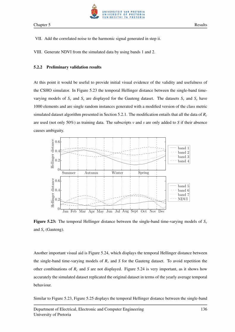
Chapter 5 Results
VII. Add the correlated noise to the harmonic signal generated in step ii.
VIII. Generate NDVI from the simulated data by using bands 1 and 2.
5.2.2 Preliminary validation results
At this point it would be useful to provide initial visual evidence of the validity and usefulness of
the CSHO simulator. In Figure 5.23 the temporal Hellinger distance between the single-band time-
varying models of Sv and Ss are displayed for the Gauteng dataset. The datasets Sv and Ss have
1000 elements and are single random instances generated with a modified version of the class metric
simulated dataset algorithm presented in Section 5.2.1. The modification entails that all the data of Rc
are used (not only 50%) as training data. The subscripts v and s are only added to S if their absence
causes ambiguity.
0
0.2
0.4
0.6
0
0.2
0.4
0.6
Hellingerdistance
band 1
band 4band 3band 2
band 5
NDVIband 7band 6
SpringAutumn WinterSummer
Jan Feb Mar Apr May Jun Jul Aug Sept Oct Nov Dec
Hellingerdistance
Figure 5.23: The temporal Hellinger distance between the single-band time-varying models of Sv
and Ss (Gauteng).
Another important visual aid is Figure 5.24, which displays the temporal Hellinger distance between
the single-band time-varying models of Rv and S for the Gauteng dataset. To avoid repetition the
other combinations of Rc and S are not displayed. Figure 5.24 is very important, as it shows how
accurately the simulated dataset replicated the original dataset in terms of the yearly average temporal
behaviour.
Similar to Figure 5.23, Figure 5.25 displays the temporal Hellinger distance between the single-band
Department of Electrical, Electronic and Computer EngineeringUniversity of Pretoria
136

Chapter 5 Results
0
0.2
0.4
0.6
0
0.2
0.4
0.6
Hellingerdistance
band 1
band 4band 3band 2
band 5
NDVIband 7band 6
SpringAutumn WinterSummer
Jan Feb Mar Apr May Jun Jul Aug Sept Oct Nov Dec
Hellingerdistance
Figure 5.24: The temporal Hellinger distance between the single-band time-varying models of Rv
and S (Gauteng).
time-varying models of Sv and Ss for the Limpopo dataset.
0
0.2
0.4
0.6
0
0.2
0.4
0.6
band 1
band 4band 3band 2
band 5
NDVIband 7band 6
SpringAutumn WinterSummer
Jan Feb Mar Apr May Jun Jul Aug Sept Oct Nov Dec
Hellingerdistance
Hellingerdistance
Figure 5.25: The temporal Hellinger distance between the single-band time-varying models of Sv
and Ss (Limpopo).
The following observations can be made when inspecting Figure 5.23, Figure 5.24 and Fi-
gure 5.25:
1. The curves in Figure 5.23 and Figure 5.9 have similar profiles. The same can be said for
Figure 5.25 and Figure 5.10.
Department of Electrical, Electronic and Computer EngineeringUniversity of Pretoria
137

Chapter 5 Results
2. The Hellinger distance for most bands in Figure 5.24 stay below 0.2. The exception is NDVI,
which stays below 0.5. For most of the year however the Hellinger distance of NDVI is close
to zero. The small Hellinger distance implies that the yearly temporal behaviour is replicated
sufficiently by the CSHO simulator. The other possible combinations of Rc and S (although not
presented) exhibit similar behaviour than that of Figure 5.24. Simular results are obtained for
the Limpopo dataset.
5.2.3 Discussion of metric selection
The metrics in this section are based on the metrics proposed in [199]. Two underlying metrics are
used, namely the Sum of Squared Error (SSE) and Hellinger distance (except for the power spectral
density metric that measures power). In both cases a value close to zero is desirable. When “Hellin-
ger” is not part of the metric name, it indicates that the SSE was used as the base metric. Each metric
was chosen to verify that the simulator reproduces three important characteristics, namely temporal
dynamics, spectral behaviour and accurate noise.
5.2.3.1 Temporal dynamics
There are two types of temporal dynamics to account for, namely intra-annual and inter-annual varia-
tion. The main reason for intra-annual variation is due to seasonality, which is caused by a wide range
of factors including plant phenology. Inter-annual variation can be caused by many factors, including
a drought or a flood. The total model error metric is a first-order statistic and is used to verify whether
the average seasonal behaviour is replicated correctly. The average temporal Hellinger distance is
probably the most important metric from the perspective of Section 4.2.3 and Section 4.3.3, as it mea-
sures the difference between the first-order statistical description of the CSHO and the true dataset.
The average temporal Hellinger distance therefore measures whether the CSHO sufficiently replicates
intra-annual variation and how effective the CSHO is in compensating for inter-annual variation. The
autocorrelation metric is a second order statistic which measures whether the CSHO also models the
temporal behaviour of any given pixel properly.
5.2.3.2 Spectral behaviour
As discussed in Section 4.1.2, the main aim of the simulator is to replicate spectral behaviour. It is
well know that each class has a unique spectral signature within a certain allowable margin of varia-
Department of Electrical, Electronic and Computer EngineeringUniversity of Pretoria
138

Chapter 5 Results
tion [39]. The proposed simulator encapsulates and models the spectral signature for each class by
using Equation 4.11. Equation 4.11 enforces the class-specific statistical restrictions imposed by the
different CSHO model parameters of each spectral band on one another. The parameter correlation
metric measures how effective the simulator is in reproducing spectral dependence (under the as-
sumption of Gaussianity), while the average parameter Hellinger distance measures how trustworthy
the joint Gaussian assumption of fc(θθθ c) is.
Furthermore, the model also enforces noise correlation by using the approach presented in Sections
4.1.2.5 and 4.1.2.6. The noise correlation metric measures how well the noise correlation is model-
led.
5.2.3.3 Accurate noise
A widely used assumption for remotely sensed time-series noise is that it is white [74, 78] if all
information-carrying frequency components have been extracted [31]. The different power spectral
density metric values reveal whether a white or coloured assumption is more appropriate when using
an SHO as the underlying deterministic model. The average noise increment Hellinger distance
determines whether the noise increments of each pixel are similar to the increments of the Ornstein-
Uhlenbeck process.
5.2.4 Class metrics
The total model error, the average parameter Hellinger distance, the parameter and noise correla-
tion and the average temporal Hellinger distance are respectively discussed in Section 5.2.4.1, Sec-
tion 5.2.4.2, Section 5.2.4.3 and Section 5.2.4.4. A few figures are presented in this section to aid
the reader in understanding the different class metrics. These figures were generated by comparing
mostly Rv and S. The dataset S used by the figures is constructed by using the same procedure detai-
led in Section 5.2.1. Again, to avoid repetition, only the graphs for the Gauteng vegetation class are
presented.
Department of Electrical, Electronic and Computer EngineeringUniversity of Pretoria
139

Chapter 5 Results
5.2.4.1 Total model error
The equation for the total model error is given by
∫ I
0‖yRc
c (t)− ySc(t)‖2
2dt, (5.4)
where yc(t) is the yearly ensemble mean of c and is defined in Equation 4.5. To determine the SSE
of each time step in the year Equation 5.4 needs to be divided by 45. To give some insight into the
total model error metric, Figure 5.26 presents the yearly ensemble means of Rv and S for the Gauteng
dataset.
0
5
10
15
20
25
30
35
40
1 2 3 4 5 6 7MODIS land bands
%R
eflec
tan
ce
Vegetation
Simulated
Figure 5.26: The yearly ensemble mean of Rv and S (Gauteng).
It is clear from Figure 5.26 that the total model error between Rv and S (for Gauteng) is close to
zero.
5.2.4.2 Average parameter Hellinger distance metric
The equation for the average parameter Hellinger distance is equal to
1|θθθ c|
|θθθ c|∑k=1
HD( f Rcc (θk), f S
c (θk)),
where fc(θk) is the marginal probability density function of fc(θθθ c) and HD( f Rcc (θk), f S
c (θk)) repre-
sents the Hellinger distance between f Rcc (θk) and f S
c (θi). Figure 5.27 ought to make the definition of
the average parameter Hellinger distance clearer. According to Figure 5.27 the parameter Hellinger
distance is greatest for A.
Department of Electrical, Electronic and Computer EngineeringUniversity of Pretoria
140

Chapter 5 Results
1
2
3
4
5
6
7
NDVI
0
C A φ λσ
Hellin
gerdistan
ce
0.1
0.2
0.3
0.4
0.5
0.6
0.7
0.8
0.9
1
Figure 5.27: HD( f Rvv (θi), f S
v (θi)) (Gauteng).
5.2.4.3 Parameter and noise correlation metrics
The equations for the noise and parameter correlation metrics are given by
‖PPPcpRc− PPPc
pS‖2
2
and
‖PPPcηRc− PPPc
ηS‖2
2.
The noise correlation metric needs to be divided by 8×8 (NDVI was added for completeness), while
the parameter correlation metric needs to be divided by 40× 40 to determine the average SSE. For
convenience the matrices PPPvpS
and PPPvηS
are displayed in Figure 5.28. There is not much difference
between Figure 5.28a and Figure 5.13a. The same goes for Figure 5.28b and Figure 5.17a.
-1
-0.5
0
0.5
1
C A φ σ λ
C
A
φ
σ
λ
(a) PPPvpS
.
-1.0
-0.5
1 2 3 4 5 6 7
1
2
3
4
5
6
7
0
0.5
1.0
NDVINDVI
(b) PPPvηS
.
Figure 5.28: PPPvpS
and PPPvηS
(Gauteng).
Department of Electrical, Electronic and Computer EngineeringUniversity of Pretoria
141

Chapter 5 Results
5.2.4.4 Average temporal Hellinger distance metric
The equation for the average temporal Hellinger distance is expressed as
18
NDVI
∑b=1
1I
∫ I
0HD( f Rc
xbc(t)
, f Sxb
c(t)) dt,
where fxbc(t) is the probability density function in band b at time step t. Figure 5.29 and Figure 5.30 are
visual aids to help explain the average temporal Hellinger distance metric. The reflectance probability
density functions at time step 3 (of 45) for all eight years in MODIS band 1 for Rv and S (Gauteng) are
displayed in Figure 5.29. The probability functions of S seem to be symmetrical about the mean (and
almost identical) of the mean values of the densities of Rv. The temporal Hellinger distance for time
steps 3+45n, n = 0, · · · ,8, in band 1 is calculated by determining the Hellinger distance between
the probability density functions in Figure 5.29. The Hellinger distance between the probability
density functions of the observation time steps of MODIS band 4 for Rv and S (Gauteng) is displayed
in Figure 5.30. The mean and variance for the curve in Figure 5.30 are respectively 0.1926 and
0.0051, which is closer to zero than one.
0 2 4 6 8 10 12 14 16 18 200
0.05
0.1
0.15
0.2
0.25
0.3
0.35
% Reflectance in MODIS band 1
Lik
elih
ood
Observed data
Simulated data
Figure 5.29: The reflectance probability density functions at time step period 3 (of 45) for all eight
years in MODIS band 1 for Rv and S (Gauteng).
5.2.5 Pixel metrics
The autocorrelation metric, the average noise increment Hellinger distance and the power spectral
density metric are respectively discussed in Section 5.2.5.1, Section 5.2.5.2 and Section 5.2.5.3. A
few figures are displayed in this section to help the reader comprehend the different pixel metrics.
Department of Electrical, Electronic and Computer EngineeringUniversity of Pretoria
142

Chapter 5 Results
0 45 90 135 180 225 270 315 3600
0.2
0.4
0.6
0.8
1
t
µ = 0.1926 σ = 0.0713
HD(f
Rv
x4 v(t),f
S x4 v(t))
Figure 5.30: The Hellinger distance between the probability density functions of the observation
time steps of MODIS band 4 for Rv and S (Gauteng).
These figures were created by comparing mostly random pixels from Rv and S . The dataset S used
to create the figures is constructed by using the same procedure described in Section 5.2.1. Again, to
avoid repetition, only the graphs for the Gauteng vegetation class are presented.
5.2.5.1 Autocorrelation metric
The autocorrelation metric is expressed mathematically as
1|Rc|
|Rc|∑p=1
∫ I
0‖RRc(p)
c (τ)− RS (p)c (τ)‖2
2 dτ, (5.5)
where RRc(p)c is the autocorrelation (defined in Equation 4.6) of the p-th pixel in Rc, while RS(p)
c is
defined similarly. To determine the average SSE per lag value Equation 5.5 needs to be divided by 368
(number of observations). Figure 5.31 displays the curves of a random vegetation pixel in Gauteng,
as well as its replicated counterpart (belonging to S ). Clearly the two curves in Figure 5.31 are very
similar.
5.2.5.2 Average noise increment Hellinger distance metric
The equation for the average noise increment Hellinger distance is defined as
18
NDVI
∑b=1
1|Rc|
|Rc|∑p=1
HD( f Rc(p)∆ηb , f S (p)
∆ηb ),
where f Rc(p)∆ηb is the density function of the noise increments ηb[t +1]−ηb[t] for pixel p in dataset Rc,
while f S (p)∆ηb is defined similarly.
Department of Electrical, Electronic and Computer EngineeringUniversity of Pretoria
143

Chapter 5 Results
0 45 90 135 180 225 270 315 360-1
-0.6
-0.20
0.2
0.6
1
τ
Simulated dataObserved data
R2 v(τ)
Figure 5.31: The autocorrelation function of a real and simulated vegetation pixel in band 2 (Gau-
teng).
5.2.5.3 Power spectral density metric
The equation for the power spectral density metric is equal to
18
NDVI
∑b=1
1|Rc|
|Rc|∑p=1
∫ 0.1
0DRη
c (p)b ( f ) d f ,
where DRηc (p)
b ( f ) is the power spectral density of the estimated noise of pixel p in dataset Rc in band
b. The same metric can be applied to S η and W η , where S η is the coloured noise (Ornstein-
Uhlenbeck) representation of Rηc (Rc after subtracting the SHO) and W η is the white noise represen-
tation of Rηc . Figure 5.32 displays DRη
v (p)2 ( f ), DS η (p)
2 ( f ) and DW η (p)2 ( f ) for a random vegetation pixel
p in the Gauteng dataset. From Figure 5.32 it is clear that∫ 0.1
0 DRηv (p)
2 ( f ) d f ≈ ∫ 0.10 DS η (p)
2 ( f ) d f ,
while∫ 0.1
0 DRηv (p)
2 ( f ) d f 6= ∫ 0.10 DW η (p)
2 ( f ) d f .
0 0.02 0.04 0.06 0.08 0.1 0.12 0.14 0.16 0.18 0.20
5000
10000
15000Observed NoiseOrnstein-UhlenbeckWhite Noise
Hz
W/H
z
Figure 5.32: The power spectral density of the estimated noise of a vegetation pixel in MODIS band
2 along with its coloured and white representations.
Department of Electrical, Electronic and Computer EngineeringUniversity of Pretoria
144

Chapter 5 Results
5.2.6 Discussion of simulator results
Random split cross-validation was performed to create 50 different class metric simulated data sets,
with the algorithm presented in Section 5.2.1 and N = 1000. No cross-validation was used for the
pixel metrics, since all the pixels in Rc were used. For the pixel metrics 50 independent experiments
were also conducted. Each data set for each experiment was independently created via the algorithm
in Section 5.2.1. The class and pixel metrics were then applied to each experiment to produce the
results in Table 5.7 and Table 5.8.
Table 5.7: Difference metrics between Rc, S and S (50 experiments) for the Gauteng dataset. The v
index indicates vegetation, while the s index indicates settlement.
Metric Name Rv Rs
Model Error 58.3917±8.1991 52.8838±22.9432
Parameter Hellinger Distance 0.1817±0.0070 0.2563±0.0081
Parameter Correlation 19.6224±3.6121 32.5042±5.7380
Noise Correlation 0.0371±0.0085 0.0629±0.0101
Temporal Hellinger Distance 0.2349±0.0042 0.2266±0.0094
Autocorrelation 31.0137±0.2431 34.3992±0.4749
Noise Hellinger Distance 0.1674±0.0003 0.1755±0.0003
Power in Rcη 92.7649 38.3202
Power in Sη 94.6440±0.6564 46.0178±0.2901
Power in Wη 22.9897±0.0642 11.7971±0.0542
The following observations can be made from Table 5.7 and Table 5.8:
1. Relative to the definitions of the SSE and Helinger distance metrics, the results in Table 5.7
and Table 5.8 are close to zero, implying that the simulator accurately replicates the temporal
dynamics and spectral characteristics of the MODIS datasets. The small variances in Table 5.7
and Table 5.8 imply that the metric results are stable and reliable.
2. Relative to the other classes the Gauteng settlement class has a higher standard deviation on its
metric results, which can be explained by the fact that the Gauteng settlement dataset is much
smaller than the other datasets.
Department of Electrical, Electronic and Computer EngineeringUniversity of Pretoria
145

Chapter 5 Results
Table 5.8: Difference metrics between Rc, S and S (50 experiments) for the Limpopo dataset. The v
index indicates vegetation, while the s index indicates settlement.
Metric Name Rv Rs
Model Error 68.5056±11.7454 56.8919±11.3777
Parameter Hellinger Distance 0.2045±0.0054 0.2097±0.0041
Parameter Correlation 15.4586±2.6663 12.9429±1.8421
Noise Correlation 0.0422±0.0063 0.0421±0.0064
Temporal Hellinger Distance 0.2147±0.0047 0.1939±0.0033
Autocorrelation 31.6738±0.1975 30.4443±0.1531
Noise Hellinger Distance 0.1630±0.0002 0.1582±0.0002
Power in Rcη 110.6438 80.5593
Power in Sη 111.0334±0.45182 85.4707±0.3112
Power in Wη 26.8485±0.0513 21.7033±0.0368
3. Relative to the metric definitions the autocorrelation metric has the largest value, which is
understandable since the non-stationarity that is present in the MODIS data shows up in the
autocorrelation metric. The error incurred due to parameter estimation also affects the autocor-
relation metric.
4. For the power metric in general Rcη ≈ Sη , while Rc
η 6=Wη , which implies that a coloured noise
model is more appropriate for the current datasets.
5. There is no standard deviation for the power in Rcη as the power of Rc
η obviously only needs to
be calculated once.
5.3 CLASSIFICATION RESULTS: GAUTENG AND LIMPOPO
The focus of this section is on the classification performance of the noise-harmonic feature group θθθ
derived from Equation 4.4 and discussed in Section 4.2.4.2. The feature group θθθ under investigation
extends the feature group ιιι proposed in [5]. The feature group θθθ is also compared with the temporal
feature group ζζζ , which is discussed in Section 4.2.4.2 [15]. The different feature groups are used
as inputs to SVM classifiers (discussed in Section 4.2.4). The SVM classifiers are also compared
Department of Electrical, Electronic and Computer EngineeringUniversity of Pretoria
146

Chapter 5 Results
with two benchmarking techniques, namely the minimum distance classifier and the time-varying
maximum likelihood classifier, which are discussed in Section 4.2.2 and Section 4.2.3 respectively.
The time-varying maximum likelihood classifier is especially important, as it is based on sequential
analysis. This section starts by introducing the different classification accuracy metrics employed,
followed by the presentation of classification results. The classification results of the Gauteng data-
set are presented in Section 5.3.3, Section 5.3.4 and Section 5.3.5. The classification results of the
Limpopo dataset are presented in Section 5.3.6.
5.3.1 Classification accuracy metrics
Two classification accuracy metrics are used in this section, namely Overall Accuracy (OA) and the κ-
coefficient. The κ-coefficient is especially useful, since it can determine whether the values contained
in an error matrix represent a result significantly better than random [200, 201]. The two metrics in
question are computed by using an error matrix, which is a matrix containing the number of pixels
classified correctly and incorrectly for each class under consideration. An example error matrix is
presented in Table 5.9.
Table 5.9: Error matrix used to explain the definition of OA and the κ-coefficient.
Class 0 Class 1
Class 0 x11 x12 x1∗
Class 1 x21 x22 x2∗
x∗1 x∗2 N
OA is a percentage (obviously the closer the metric is to 100 the better the classifier) and is defined
as
100×r
∑i=1
xii/N, (5.6)
while the κ-coefficient is computed with
κ =N ∑
ri=1 xii−∑
ri=1 xi∗× x∗i
N2−∑ri=1 xi∗× x∗i
. (5.7)
In Equation 5.6 and Equation 5.7, N is the total number of pixels in the error matrix, r is the number
of rows in the matrix, xii is the number in row i and column i, xi∗ is the total for row i, and x∗i is
the total for column i (see Table 5.9 for more details). Note that x11 refers to the number of pixels
belonging to class 0 classified correctly and x22 refers to the number of pixels belonging to class
Department of Electrical, Electronic and Computer EngineeringUniversity of Pretoria
147

Chapter 5 Results
1 which were classified correctly, while x21 refers to the number of pixels belonging to class 0
which were not classified correctly and x12 refers to the number of pixels belonging to class 1 which
where not classified correctly. The value of κ can be smaller than or equal to 1. The magnitude
guidelines for κ published in [202] are adopted here. According to [202], a larger κ indicates that the
classifier can easily discern the different classes, while a smaller (or even negative) κ indicates that
the classifier cannot easily discern the different classes.
5.3.2 Structure used for accuracy metrics
In this section a three-dimensional structure is presented that is used to organise the cross-validation
classification results of Section 5.3.3 to Section 5.3.7.
The κ-coefficients and the OA percentages generated by the cross-validation experiments in Sec-
tion 5.3.3 to Section 5.3.6 can be organised into a three-dimensional irregular structure Ξυ ,µ ,
where
υ ∈ ‘κ’, ‘OA’
and
µ ∈ Min Dist,TVML,θθθ , ιιι ,ζζζ (5.8)
with elements
ξµ
x,y(x),z ∈ κ ,OA,
where
x ∈ 1,2, · · · ,8;
y(x) ∈
1,2, · · · ,(
x8
);
z ∈ 1,2, · · · ,e. (5.9)
In Equation 5.8, Min Dist,TVML,θθθ , ιιι and ζζζ are respectively associated with the minimum distance
classifier, the time-varying maximum likelihood classifier, the noise-harmonic feature group, the har-
monic feature group and the temporal feature group defined in Section 4.2.4.2. When µ is omitted it
implies that the classification procedure that generated Ξυ is unknown.
Department of Electrical, Electronic and Computer EngineeringUniversity of Pretoria
148

Chapter 5 Results
In Equation 5.9, x represents the band restriction value (the amount of bands that may be used for
classification), while each y is associated with a unique band combination given the restriction of x
(which explains the combination notation used to define y). The z index points to a specific cross-
validation experiment and e ∈ 1,2, · · · denotes the amount of experiments performed.
Recall that each MODIS pixel consists of a time-series. The notation Ξυ [n] should be interpreted as
representing a structure similar to Ξυ , with the only difference being that it consists of classification
accuracy metric elements obtained by using truncated (n ∈ 1,2, · · · ,368) MODIS pixels. It should
be clear that if [n] is omitted from Ξυ [n] then it implies that no truncation was performed before
classification commenced.
The notation Φυ = Eω [Ξυ ] should be interpreted as the sample mean of Ξυ along the dimension
ω ∈ x,y,z (which is similar to the Matlab mean command). The resulting structure Φυ has only
two dimensions, since Eω [] eliminated a dimension of Ξυ . The notation Θυ = Eη 6=ω [Eω [Ξυ ]] should
be interpreted as the sample mean of Ξυ along the dimension ω , followed by the sample mean of Φυ
along the dimension η ∈ x,y,z. Note that the resulting structure Θυ has only one dimension. The
structures σωΞυ and ση 6=ωσωΞυ should be interpreted in a similar way, except for the fact
that σ indicates that standard deviation (which is similar to the Matlab std command) should be used
instead of the sample mean when deriving σωΞυ and ση 6=ωσωΞυ. The notation
Συ = Ξ1,2,··· ,7,∗,1υ
should be interpreted as a substructure of Ξυ which only contains the elements in Ξυ for which
x = 1,2, · · · ,7 and z = 1. The ∗ is a wild card which indicates all valid values y can ascertain.
If one of the dimensions of a structure Συ is equal to one, then (Συ)@ should be interpreted as the
structure obtained after the redundant dimension is removed. When two structures Ξυ ,µ1 and Ξυ ,µ2
are compared, then classification approach µ1 performs better than µ2 if ξµ1x,y(x),z > ξ
µ2x,y(x),z for more
than 50% of all the possible index values (see Equation 5.9).
5.3.3 Preliminary benchmark classification results: Gauteng
In this section the results of the benchmark classification approaches are presented. The benchmark
classifiers that were used are the minimum distance classifier and the time-varying maximum likeli-
hood classifier presented in Section 4.2.2 and Section 4.2.3 respectively [23]. These two approaches
were selected, as they are frontier hypertemporal approaches. As the algorithms are only used for
Department of Electrical, Electronic and Computer EngineeringUniversity of Pretoria
149

Chapter 5 Results
benchmarking, the full vegetation and settlement datasets were used for training and validation (im-
plying that e = 1). The estimation procedure for the yearly ensemble means used by the minimum
distance classifier is discussed in Section 5.1.1, while the estimation of the time-varying model used
by the time-varying maximum likelihood classifier is discussed in Section 5.1.2. Moreover, no se-
quential thresholds were used for the time-varying maximum likelihood classifier and π = 0.5. The
OA classification results of the benchmarking approaches for each possible band combination are
found in Figure 5.33.
1 2 3 4 5 6 7
10
20
30
40
50
60
70
Number of bands
Number
ofcombinations
OA%
50
60
70
80
90
100
(a)(
Ξ1,2,··· ,7,∗,1‘OA’,Min Dist
)@.
50
60
70
80
90
100
1 2 3 4 5 6 7
10
20
30
40
50
60
70
Number of bands
Number
ofcombinations
OA%
(b)(
Ξ1,2,··· ,7,∗,1‘OA’,TVML
)@.
Figure 5.33: The classification results (OA) of the benchmarking approaches of the Gauteng dataset.
Each possible two-band combination κ-coefficient for the benchmarking approaches is presented in
Figure 5.34.
The following observations and conclusions can be made from Figure 5.34:
1. With respect to the minimum distance classifier, the bands that in combination perform best are
2,4,7,NDVI, while bands 1,3,5,6 perform worst (in terms of classification capability).
The band that in combination performs best is band 2, while band 5 performs worst. The band
combination that separates the two classes best is 4,7, while the lowest κ value is produced
by 1,5.
2. The results are exactly the same for the time-varying maximum likelihood classifier, except
that 4,6 is the band combination that performs best, while band combination 1,3 performs
worst.
3. For both approaches NDVI performs best (single-band). The worst performing bands are res-
Department of Electrical, Electronic and Computer EngineeringUniversity of Pretoria
150

Chapter 5 Results
NDVI
1 2 3 4 5 6 7
1
2
34
5
6
7
NDVIAVG
κC
oeffi
cient
AVG 0.1
0.20.30.40.50.60.70.80.9
(a)(
Ξ1,2,∗,1‘κ’,Min Dist
)@packed into a symmetrical matrix
(plus a mean row and column).
NDVI
1 2 3 4 5 6 7
1
2
34
5
6
7
NDVIAVG
κC
oeffi
cient
AVG 0.1
0.20.30.40.50.60.70.80.9
(b)(
Ξ1,2,∗,1‘κ’,TVML
)@packed into a symmetrical matrix (plus
a mean row and column).
Figure 5.34: The two-band classification results (κ) of the benchmarking approaches of the Gauteng
dataset.
pectively band 5 and 6 in the case of the minimum distance classifier and the time-varying
maximum likelihood classifier.
4. Recall from Section 5.1.2.3 that the temporal Hellinger metric predicted that a temporal clas-
sifier using bands 1,2,3,4 would perform better than a temporal classifier using bands
5,6,7,NDVI. As seen in Figure 5.34, this prediction is reasonably close to the actual ob-
served behaviour of the two temporal benchmarking classifiers investigated in this section. A
possible reason for the discrepancy between the observed behaviour and the predicted beha-
viour is discussed in Section 5.3.4.
5. Generally the time-varying maximum likelihood classifier outperforms the minimum distance
classifier, as it uses a superior metric, namely the posterior sequence, which incorporates the
yearly ensemble mean as well as the inter-class variance.
As an interesting side note, a closer look is taken at bands 4,7 and 1,5 from Figure 5.34a.
The yearly ensemble means (after fitting appropriate sinusoids) of 4,7 and 1,5 are displayed in
Figure 5.35a and Figure 5.35b, respectively. It is clear from Figure 5.35 that, in the case of bands
4 and 7, the yearly ensemble means of the settlement and vegetation classes have a greater distance
between them than in bands 1 and 5. The increased distance observable when inspecting the yearly
ensemble means of 4,7 and 1,5 helps to explain why the minimum distance classifier using
bands 4,7 outperforms the minimum distance classifier using bands 1,5.
Department of Electrical, Electronic and Computer EngineeringUniversity of Pretoria
151

Chapter 5 Results
% Reflectance (land band 1)
%R
efl
ecta
nce
(lan
db
an
d5)
7 8 9 10 11 12 1322
26
30
34Vegetation
Settlements
(a) Yearly ensemble mean models of bands 1 and 5.
6.5 7.5 8.5 9.5 10.513
15
17
19
21
23
% Reflectance (land band 4)
%R
efl
ecta
nce
(lan
dband
7)
Vegetation
Settlements
(b) Yearly ensemble mean models of bands 4 and 7.
Figure 5.35: Two-dimensional yearly ensemble mean models of Gauteng.
In the last part of this section the focus will shift to the time-varying maximum likelihood classifier.
The time-varying maximum likelihood classifier is unique in the sense that it is based on sequential
analysis (discussed in Section 3.4) and was first introduced (to the remote sensing field) in [23]. As the
time-varying maximum likelihood classifier is based on sequential analysis it can be truncated, which
allows the classifier to make a decision after each observation is received by using all the observations
received up to that point. The focus of [23] was on the trade-off between classification accuracy and
classification delay. The classification study in Section 5.3 however focused solely on increasing
classification accuracy. One of the aims of this thesis, which was stated in Chapter 1, is to verify the
sequential results presented in [23]. The most important result of [23] was therefore reproduced and
can be found in Figure 5.36. Figure 5.36 presents the mean single-band classification κ-coefficient or
average single-band classification performance of the time-varying maximum likelihood classifier as
a function of time or sample size. If the notation from Section 5.3.2 is used then the mean single-band
classification κ-coefficient (as a function of sample size) can be expressed as
Ey(1)
[(Ξ
1,∗,1‘κ’,Min Dist[n]
)@].
The delay and accuracy measures discussed in Section 4.2.3 are not calculated, as the datasets under
consideration have finite sizes and Figure 5.36 thus displays an alternative fixed-sample-size perfor-
mance measure.
Generally the average κ-coefficient in Figure 5.36 increases with time. A steep increase is observable
in the first year and a smaller increase during the second year. After the second year however the
increase of κ is small. The temporal dynamics of the average κ-coefficient in Figure 5.36 suggests that
Department of Electrical, Electronic and Computer EngineeringUniversity of Pretoria
152

Chapter 5 Results
2002 2003 2004 2005 2006 2007 2008 20090.35
0.45
0.55
0.65
0.75
2001
Ave
rage
κ-c
oeffi
cien
t
Figure 5.36: The average single-band classification performance of the time-varying maximum like-
lihood classifier for the Gauteng dataset as a function of time.
for the Gauteng dataset specifically the thresholds of the time-varying maximum likelihood classifier
should be chosen in such a way that the classifier on average experiences (excluding outliers) at least
a one-year delay (preferably two) before it can classify an observed sequence. The same result was
obtained in another independent study, namely [78].
5.3.4 Preliminary SVM classification results: Gauteng
The SVM classifier and the proposed feature groups are discussed in Section 4.2.4 and Section 4.2.4.2
respectively. Recall from Section 4.2.4.2 that three feature groups are proposed, namely temporal fea-
tures ζζζ , harmonic features ιιι and noise-harmonic features θθθ . A linear SVM is used, since it produced
sufficient classification results. The SVM is realised with the SVM and Kernel Methods Matlab Tool-
box [203]. The SVM and Kernel Methods Matlab Toolbox requires two input parameters, which
are determined via a standard grid search algorithm. The two input parameters that need to be set
are (c,λ ). The parameter c sets the bound on the Lagrangian multipliers, while λ is a conditioning
parameter for the quadratic programming method used to determine the SVM hyperplane. Random
split cross-validation (50% for training and 50% for validation) was employed by the grid search al-
gorithm (50 independent experiments). The cross-validation OA results of the Gauteng dataset for all
the possible band combinations of ζζζ , ιιι and θθθ are presented in Figure 5.37. The standard deviation in
Figure 5.37 for each feature group is small, indicating that the classification results are reliable and
stable.
The Gauteng two-band classification results for ζζζ , ιιι and θθθ are presented in Figure 5.38. The κ-
Department of Electrical, Electronic and Computer EngineeringUniversity of Pretoria
153

Chapter 5 Results
1 2 3 4 5 6 7
10
20
30
40
50
60
70
Number of bands
Number
ofcombination
s
OA%
50
60
70
80
90
100
(a) Gauteng: Ez
[Ξ1,2,··· ,7,∗,∗‘OA’,ζζζ
].
1 2 3 4 5 6 7
10
20
30
40
50
60
70
Number of bands
Number
ofcombinations
σOA
0.5
1
1.5
2
2.5
(b) Gauteng: σz
Ξ1,2,··· ,7,∗,∗‘OA’,ζζζ
.
50
60
70
80
90
100
1 2 3 4 5 6 7
10
20
30
40
50
60
70
Number of bands
Number
ofcombinations
OA%
(c) Gauteng: Ez
[Ξ1,2,··· ,7,∗,∗‘OA’,ιιι
].
1 2 3 4 5 6 7
10
20
30
40
50
60
70
Number of bands
Number
ofcombinations
σOA
0.5
1
1.5
2
2.5
(d) Gauteng: σz
Ξ1,2,··· ,7,∗,∗‘OA’,ιιι
.
1 2 3 4 5 6 7
10
20
30
40
50
60
70
Number of bands
Number
ofcombinations
OA%
50
60
70
80
90
100
(e) Gauteng: Ez
[Ξ1,2,··· ,7,∗,∗‘OA’,θθθ
].
1 2 3 4 5 6 7
10
20
30
40
50
60
70
Number of bands
Number
ofcombinations
σOA
0.5
1
1.5
2
2.5
(f) Gauteng: σz
Ξ1,2,··· ,7,∗,∗‘OA’,θθθ
.
Figure 5.37: The cross-validation results [with (∞,0.05) and e = 50] of the Gauteng dataset for all
the possible band combinations of ζζζ , ιιι and θθθ .
Department of Electrical, Electronic and Computer EngineeringUniversity of Pretoria
154

Chapter 5 Results
NDVI
1 2 3 4 5 6 7
1
2
34
5
6
7
NDVIAVG
κC
oeffi
cient
AVG 0.1
0.20.30.40.50.60.70.80.9
(a) Gauteng: Ez
[Ξ1,2,∗,∗‘κ’,ζζζ
]packed into a symmetrical ma-
trix.
NDVI
1 2 3 4 5 6 7
1
2
34
5
6
7
NDVIAVG
κC
oeffi
cient
AVG 0.1
0.20.30.40.50.60.70.80.9
(b) Gauteng: Ez
[Ξ1,2,∗,∗‘κ’,ιιι
]packed into a symmetrical ma-
trix.
NDVI
1 2 3 4 5 6 7
1
2
34
5
6
7
NDVIAVG
κC
oeffi
cient
AVG 0.1
0.20.30.40.50.60.70.80.9
(c) Gauteng: Ez
[Ξ1,2,∗,∗‘κ’,θθθ
]packed into a symmetrical ma-
trix.
NDVI
1 2 3 4 5 6 7
1
2
34
5
6
7
NDVIAVG
κC
oeffi
cient
AVG 0.1
0.20.30.40.50.60.70.80.9
(d) Average between ζζζ , ιιι and θθθ results for Gauteng.
Figure 5.38: The two-band classification results (average κ) of ζζζ , ιιι and θθθ for the Gauteng dataset
[with (∞,0.05) and e = 50].
coefficients reported in Figure 5.38 are the average of 50 random split cross-validation experiments.
The following observations and conclusions can be made from Figure 5.38:
1. When the SVM classifier using ζζζ uses data from bands 1,2,4,6 it classifies better than when
the SVM classifier using ζζζ uses data from bands 3,5,7,NDVI. The SVM classifier using ζζζ
obtains its best classification results when data from band 2 are used in combination, while the
SVM classifier using ζζζ performs at its worst when data from band 5 are used in combination.
The two-band combination 2,5 performs best, while the two-band combination 7,NDVIperforms worst of all the two-band combinations. The best and worst single-bands that the
SVM classifier using ζζζ can use are bands 2 and 5 respectively.
2. When the SVM using the harmonic features ιιι uses data from bands 1,2,7,NDVI it achieves
Department of Electrical, Electronic and Computer EngineeringUniversity of Pretoria
155

Chapter 5 Results
better classification results than when it uses data from bands 3,4,5,6. When the SVM using
the harmonic features ιιι use data from band 7 in combination it produces the best classification
results, while using band 5 in combination leads to the worst classification results. Band com-
bination 3,5 performs best, while band combination 2,7 performs worst of all the possible
two-band combination. The best and worst single-bands that the SVM classifier using ιιι can
use are NDVI and band 5 respectively.
3. The SVM using the noise-harmonic features θθθ perform better when it uses data from bands
1,2,4,7 than when it uses data from bands 3,5,6,NDVI. The highest average κ values are
achieved when band 2 is used in combination, while the lowest average κ values are achieved
when using band 3 in combination. The two-band combination that perform best is 1,2,while 3,4 perform the worst among all the possible two-band combinations. The best and
worst single-bands that the SVM classifier using θθθ can use are bands 2 and 3 respectively.
4. Generally for the Gauteng dataset, the SVM using θθθ outperforms the SVMs using ζζζ and ιιι . The
SVM using ιιι outperforms the SVM using ζζζ . The fact that the feature group θθθ outperforms ιιι is
as expected, since the parameter Hellinger distance indicated in Section 5.1.3.3 that the noise
and phase parameters of the CSHO are extra discerning features, which implies that they can
be used to extend the classification potential of ιιι .
5. The average κ-coefficients of the SVMs using ζζζ , ιιι and θθθ are presented in Figure 5.38d, from
which it is clear that on average combining 1,2,3,4 with 6,7,NDVI produces high κ
values. Furthermore, generally the following band combinations, 1,2,5,2 and 3,2, also
perform well.
6. Recall from Section 5.1.2.3 that for the Gauteng dataset the temporal Hellinger distance metric
predicted that a classifier using data from bands 1,2,3,4 would provide better class differen-
tiability than a classifier using data from bands 5,6, 7,NDVI when the classifier in question
relies on temporal features. Similarly, recall from Section 5.1.3.3 that the parameter Hellinger
distance metric predicted that a classifier using data from bands 1,2,7,NDVI would provide
better class differentiability than a classifier using bands 3,4,5,6 when the classifier in ques-
tion employs the parameters of the CSHO as classification features. As seen in Figure 5.38,
these two predictions are close to the actual observed behaviour of the three SVM classifiers
investigated in this section. The correlation between the predictions and reality implies that the
Department of Electrical, Electronic and Computer EngineeringUniversity of Pretoria
156

Chapter 5 Results
separability metrics introduced in Section 5.1 can be used to select classification features. The
small discrepancy between the observed behaviour and the predicted behaviour can be ascribed
to the fact that the relation between actual performance and predicted separability based on
a single metric is not a perfect one-to-one relation, as the single metric does not incorporate
all the factors (for instance spectral dependence is not measured by the Hellinger metric) that
influence the performance of a specific classifier.
5.3.5 Classification results: Gauteng
Finally, the bar graph representing the Ey(x)[Ez[Ξ‘κ’,µ
]]values for each classification approach men-
tioned (for all µ) is presented in Figure 5.39. Note that there is no cross-validation experiments for
the benchmarking approaches. In the case of the benchmarking approaches only one sample mean is
taken over all the band combinations. The values Ey(x)[σz
Ξ‘κ’,µ]
for the SVM approaches are dis-
played in Figure 5.39b. Recall that the index x ∈ 1,2, · · · ,8 is used to indicate the band restriction
value. So if x = 5, the band restriction value is equal to 5. The following observations can be made
from Figure 5.39a and Figure 5.39b:
1. The SVM classifier using the noise-harmonic features outperform all the other classifiers when
x ≤ 3. When x > 3 however the time-varying maximum likelihood classifier performs bet-
ter than the SVM classifier using the noise-harmonic features. Furthermore, when x > 3 the
SVM classifier using the harmonic features produces similar classification results as the SVM
classifier using the noise-harmonic features.
2. For all values of x, the time-varying maximum likelihood classifier on average achieves hi-
gher classification accuracies compared to the remaining classifiers (when the SVM using θθθ is
excluded).
3. The SVM classifier using the harmonic features classifies better than the SVM using ζζζ and the
minimum distance classifier except when x = 1, then ζζζ produces better classification results
than ιιι or the minimum distance classifier.
4. The SVM classifier using the temporal features outperforms the minimum distance classifier
when x < 8. When x = 8 the minimum distance classifier outperforms the SVM using ζζζ .
5. For all classifiers, increasing the spectral dimension increases classification accuracy.
Department of Electrical, Electronic and Computer EngineeringUniversity of Pretoria
157

Chapter 5 Results
6. The standard deviation for each SVM classifier (for all x) is small, implying that the classifica-
tion results are stable and reliable.
TVML ζ ι θ0
0.2
0.4
0.6
0.8
1
1 band
2 bands
3 bands
4 bands
5 bands
6 bands
7 bands
8 bands
MinDist
E y(x
)
[ E z[ Ξ
‘κ’,µ
]]
(a) Ey(x)[Ez[Ξ‘κ’,µ
]]for the Gauteng dataset.
0
0.005
0.01
0.015
ζ ι θ
1 band
2 bands
3 bands
4 bands
5 bands
6 bands
7 bands
8 bands
E y(x
)
[ σz
Ξ‘κ’,µ
](b) Ey(x)
[σz
Ξ‘κ’,µ]
for the Gauteng dataset.
Figure 5.39: The bar graph representing the Ey(x)[Ez[Ξ‘κ’,µ
]]values for the benchmarking and SVM
classifiers [with (∞,0.05) and e = 50] (Gauteng).
5.3.6 Classification results: Limpopo
To avoid repetition, only the most important classification results for the Limpopo data set will be
mentioned. As mentioned in Section 5.3.3, the time-varying maximum likelihood classifier is an
important facet of the thesis and the equivalent of Figure 5.36 is therefore presented in Figure 5.40
for the Limpopo dataset.
2002 2003 2004 2005 2006 2007 2008 20090.35
0.45
0.55
0.65
0.75
2001
Ave
rage
κ-c
oeffi
cien
t
Figure 5.40: The average single-band classification performance of the time-varying maximum like-
lihood classifier for the Limpopo dataset as a function of time.
Department of Electrical, Electronic and Computer EngineeringUniversity of Pretoria
158

Chapter 5 Results
Generally the average κ-coefficient in Figure 5.40 increases during the first two years. A steep in-
crease is observable in the first year and a smaller increase during the second year. After the second
year however the average κ-coefficient starts to decrease steadily. The temporal dynamics over the
first two years of the average κ-coefficient in Figure 5.40 strengthens the one-year (preferably two-
year) sequential detection delay rule formed in Section 5.3.3, while inspecting Figure 5.36. The
behaviour in Figure 5.36 and Figure 5.40 however differs from 2002 onwards. The decrease in κ ob-
servable in Figure 5.40 implies that the vegetation and settlement classes in the case of the Limpopo
dataset become less separable over time. The opposite behaviour is seen in Figure 5.36, implying that
the separability does not decrease in the case of the Gauteng dataset. The loss in separability in the
case of the Limpopo dataset is not directly observable when inspecting Table 5.8, which implies that
the separability loss happens gradually.
The equivalent of Figure 5.39 is presented in Figure 5.41 for the Limpopo dataset, as it sums up the
performance of each classifier on the Limpopo dataset. As mentioned in Section 5.3.4, a grid search
is required to obtain the SVM software parameters (c,λ ). Random split cross-validation (50% for
training and 50% for validation) was also employed by the grid search algorithm for the Limpopo da-
taset (10 independent experiments). The content details of Figure 5.41 are discussed in Section 5.3.5.
Also recall from Section 5.3.5 that x ∈ 1,2,8 indicates the band restriction value.
0
0.2
0.4
0.6
0.8
11 band
2 bands
8 bands
TVML ζ ι θMinDist
E y(x
)
[ E z[ Ξ1,2,8,∗,∗
‘κ’,µ
]]
(a) Ey(x)[Ez[Ξ1,2,8,∗,∗‘κ’,µ
]]for the Limpopo dataset.
0
0.005
0.01
0.015
ζ ι θ
Ey(x
)
[ σz
Ξ1,2,8,∗,∗
‘κ’,µ
]
1 band
2 bands
8 bands
(b) Ey(x)[σz
Ξ1,2,8,∗,∗‘κ’,µ
]for the Limpopo dataset.
Figure 5.41: The bar graph representing the Ey(x)[Ez[Ξ‘κ’,µ
]]values for the benchmarking and SVM
classifiers [with (∞,1) and e = 10] (Limpopo).
The following observations can be made from Figure 5.41:
Department of Electrical, Electronic and Computer EngineeringUniversity of Pretoria
159

Chapter 5 Results
1. The SVM classifier using the noise-harmonic features on average achieves higher classification
accuracies than any of the other classifiers for all x.
2. The SVM classifier using the temporal features on average produces better classification results
if compared to all the classification results produced by the remaining classifiers (if the SVM
classifier using θθθ is excluded) except when x = 8. When x = 8 the SVM classifier using ιιι
outperforms the SVM using ζζζ .
3. The time-varying maximum likelihood classifier and the SVM classifier using the harmonic
features on average achieve better classification accuracies if compared with the classification
results produced by the minimum distance classifier.
4. When x = 1 or x = 8 the SVM using the harmonic features outperforms the time-varying maxi-
mum likelihood classifier. When x = 2 exactly the opposite behaviour is observed.
5. For all classifiers, increasing the spectral dimension improves the accuracy of the classifier.
6. The standard deviation for each SVM classifier (for all x) is small, implying that the classifica-
tion results are reliable and stable.
7. According to the classification results the Limpopo dataset is less separable than the Gauteng
dataset.
5.3.7 Important classification conclusions
The following important conclusions can be made from the results presented in Section 5.3:
1. As the conclusions in Section 5.3.3 and Section 5.3.4 show, the metrics proposed in Section 5.1
can be used to choose efficient spectral bands and classification features.
2. As mentioned in Section 5.3.5 and Section 5.3.6, increasing the spectral dimension of a classi-
fier improves its classification accuracy.
3. The feature group θθθ is an extension of ιιι , not only in size but also in terms of its classifica-
tion capability. This is clearly seen in Figure 5.11, Figure 5.14 and Figure 5.38. Moreover,
Figure 5.39 and Figure 5.41 show that the SVM classifier that uses θθθ outperforms all the other
Department of Electrical, Electronic and Computer EngineeringUniversity of Pretoria
160

Chapter 5 Results
classifiers investigated (except when x > 2, in the case of the Gauteng datset, which is when
the time-varying maximum likelihood classifier starts achieving a slightly better classification
accuracy). It is also significant to mention that the SVM classifier using θθθ performs much bet-
ter than the other classifiers when the spectral dimension of the classifier is low. This unique
characteristic of θθθ is significant, since it is obviously more advantageous to classify more ac-
curately without having to increase the spectral view.
4. The Limpopo dataset is less separable than the Gauteng dataset, according to the classification
results in Section 5.3.5 and Section 5.3.6. This is not surprising for the temporal or the CSHO
feature classifiers. Even though the temporal Hellinger distance metrics in Table 5.3, are similar
for the Gauteng and Limpopo datasets it is clear from Figure 5.40 that the separability of the
Limpopo dataset deteriorates over time, explaining the weaker performance (in the case of the
Limpopo dataset) of the minimum distance classifier, the time-varying maximum likelihood
classifier and the SVM using ζζζ in spite of good separability in the time-varying models of the
Limpopo dataset. For ιιι and θθθ it is clear from Figure 5.11 and Figure 5.14 that the parameters
of the CSHO provide better classification capability in the case of the Gauteng dataset than for
the Limpopo dataset.
5. The most important sequential result found in [23] was reproduced, which is stated next. The
temporal dynamics of the average κ-coefficient in Figure 5.36 and Figure 5.40 suggest that in
general the thresholds of the time-varying maximum likelihood classifier should be chosen in
such a way that the classifier on average experiences (excluding outliers) at least a one-year
delay (preferably two) before it can classify an observed sequence.
5.4 CHANGE DETECTION RESULTS: GAUTENG AND LIMPOPO
This section focuses on the performance of the sequential change detection algorithm presented in
Section 4.3.3, namely CUSUM. The CUSUM algorithm is benchmarked against the popular band
differencing algorithm discussed in Section 4.3.2. This section starts by introducing the different
change detection metrics employed, followed by the presentation of the change detection results of
band differencing and CUSUM.
Department of Electrical, Electronic and Computer EngineeringUniversity of Pretoria
161

Chapter 5 Results
5.4.1 Change detection accuracy metrics
As change detection metrics PD, PFA, E(T −τ)+368 and Ae are employed as metrics instead of dl(T )
and f (T ), which were introduced in Section 3.6, since metrics that can be fairly compared to non-
sequential change detection algorithms are required. Here PD is the probability of correctly detecting
a change within the eight-year observation period, PFA is the probability of detecting a change when
there was no change in the eight-year period, E(T − τ)+368= EminmaxT − τ,0,368− τ is
the positive expected delay truncated to 368 observations and Ae =12 [(1−PD)+PFA].
5.4.2 Results of Lunetta et al.’s scheme: Gauteng and Limpopo
The scheme developed by Lunetta et al. is discussed in detail in Section 4.3.2 and is also known as
the band differencing algorithm [7]. The band differencing algorithm is a popular time-series change
detection benchmarking method, which requires two parameters as input, the amount of frequency
components ν to preserve and the decision threshold hbl [10,28]. A grid search was performed to find
suitable values for ν and hbl . In this section the algorithm is applied to the Gauteng and Limpopo
datasets. The values for ν , hbl and the change detection accuracies can be found in Table 5.10 and
Table 5.11 for the Gauteng and Limpopo datasets, respectively. As the band differencing approach is
used for benchmarking, the entire Gauteng and Limpopo datasets are used for training and validation.
In a previous study [30], the band differencing algorithm was applied to the Gauteng and Limpopo
datasets. In [30], the focus was on preserving the structure of the original signal and for that reason
ν was set equal to 10. Figure 5.42 displays the effect of ν , which should make the reason for setting
ν equal to 10 in the previous study clear. In this section, however the structure of the original signal
is not one of the design criteria, and ν is thus found via a grid search algorithm. The number of
frequency components ν to keep (as found via the grid search algorithm) is respectively set to two
and three for the Gauteng and Limpopo datasets.
The following observations and conclusions can be made from Table 5.10 and Table 5.11:
1. In Table 5.10 and Table 5.11 the lower value of ν increases the accuracy of the band differencing
change detector. The remaining observations assume that the lower value of ν is used.
2. For the Gauteng dataset it is clear from Table 5.10 that when the band differencing algorithm
employs bands 1,3,4,NDVI the accuracy of the band differencing change detector is higher
Department of Electrical, Electronic and Computer EngineeringUniversity of Pretoria
162

Chapter 5 Results
0
20
40
2001 2002 2003 2004 2005 2006 2007 2008 2009
band 1
band 4band 3band 2
band 5
band 7band 6
A MODIS vegetation pixel in the Gauteng dataset
0
20
40
0
20
40
A filtered version of the above pixel (ν = 2)
A filtered version of the above pixel (ν = 10)
%R
eflec
tance
Figure 5.42: A true vegetation pixel belonging to the Gauteng dataset and two different filtered
versions of the vegetation pixel.
than if it uses bands 2,5,6,7. Using band 1 leads to the lowest average error Ae, while using
band 5 leads to the highest average error.
3. Exactly the same performance is observable for the Limpopo dataset as for the Gauteng dataset,
except that for the Limpopo dataset, using band 4 leads to the lowest average error, while using
band 2 leads to the highest average error.
4. Generally the Gauteng dataset produces lower average errors when it is compared with the
Limpopo dataset.
5.4.3 Temporal dependence and the CUSUM threshold
The influence of temporal dependence on the CUSUM threshold needs to be investigated before
CUSUM can be applied to MODIS data. The influence of temporal dependence on the CUSUM
threshold is explained in this section with the aid of an example. Assume therefore that there is a
sequence zk which is an i.i.d. sequence. The sequence is drawn independently from q0 before change
point τ and from τ onwards drawn from q1. The density q0 ∼N (0,1) and the density q1 ∼N (1,1).
An example of such a sequence can be found in Figure 5.43a with τ = 64. The CUSUM statistic
gk generated from zk with Equation 3.55 when y = 0 in Equation 3.55 is displayed in Figure 5.43c.
Note that Equation 3.55 employs the log likelihood ratio sk defined in Equation 3.56. While gk stays
Department of Electrical, Electronic and Computer EngineeringUniversity of Pretoria
163

Chapter 5 Results
1 10 20 30 40 50 60 70 80 90 100-4
-3
-2
-1
0
1
2
3
4
τ = 64
k
zk
-4 -3 -2 -1 0 1 2 3 4 50
0.1
0.2
0.3
0.4
0.5
zk before and after change point τ
Likelihood
q0 q1
(a) zk is independent.
-5
-4
-3
-2
-1
0
1
2
3
τ = 71
zk
-4 -3 -2 -1 0 1 2 3 4 50
0.1
0.2
0.3
0.4
0.5
zk before and after change point τ
Likelihood
q0 q1
1 10 20 30 40 50 60 70 80 90 100k
(b) zk is not independent.
1 10 20 30 40 50 60 70 80 90 1000
2
4
6
8
10
12
14
16
18
k
gk
-4 -3 -2 -1 0 1 2 3 4 5
0.1
0.2
0.3
0.4
0.5
sk before and after change point τ
Likelihood
f0 f1
0
(c) gk for independent case.
1 10 20 30 40 50 60 70 80 90 1000
2
4
6
8
10
12
14
16
18
k
gk
-4 -3 -2 -1 0 1 2 3 4 5
0.1
0.2
0.3
0.4
0.5
sk before and after change point τ
Likelihood
f0 f1
0
(d) gk for dependent case.
Figure 5.43: gk for an independent and dependent example.
Department of Electrical, Electronic and Computer EngineeringUniversity of Pretoria
164

Chapter 5 Results
Table 5.10: Band differencing applied to the Gauteng dataset.
MODIS band hbl PD PFA Ae
ν=2ν=10
1 1.25981.8874
0.79010.6133
0.06930.2247
0.13960.3057
2 1.36990.7477
0.60770.9613
0.17740.8986
0.28480.4687
3 1.18271.5350
0.77350.7790
0.12330.3919
0.17490.3064
4 1.25981.5681
0.77350.7182
0.05910.3311
0.14280.3064
5 1.46350.7918
0.53590.9392
0.20100.8733
0.33260.4670
6 1.54602.7407
0.57460.2210
0.12330.0591
0.27440.4191
7 1.27631.7222
0.69610.6796
0.14700.2787
0.22540.2996
NDVI 1.20471.5185
0.80110.8122
0.16220.4645
0.18050.3262
below a threshold h no change is declared. After crossing the threshold h a change is declared. If
zk is associated with q0 and q1 then sk will be associated with f0 ∼ N (−12 ,1) and f1 ∼ N (1
2 ,1)
because
sk = lnq1(zk)
q0(zk)
= lne−
12 (zk−1)2
e−12 z2
k
= zk−12.
The densities f0 and f1 are displayed in Figure 5.43c.
The focus now shifts to the discretised Ornstein-Uhlenbeck process (see Section 4.1.2.1), which is a
dependent sequence with generating equation
zk = e−λ zk−1 +(1− e−λ )µ +σ
√1− e−2λ
2ληk,
where λ > 0 determines the degree of dependence (as well as the mean reversion rate), µ is the
long-term mean, σ > 0 is the volatility of the random fluctuations and ηk is i.i.d. and has density
N (0,1). Recall from Section 4.1.2.1 that the dependent sequence zk is distributed according to den-
sity N(µ, σ2
2λ
)(the equilibrium density) as long as z0 is also distributed according to the equilibrium
density. The closer λ gets to zero the higher the temporal dependence in the sequence zk. To mi-
Department of Electrical, Electronic and Computer EngineeringUniversity of Pretoria
165

Chapter 5 Results
Table 5.11: Band differencing applied to the Limpopo dataset.
MODIS band hbl PD PFA Ae
ν=3ν=10
1 2.22872.4379
0.64960.4957
0.08220.0788
0.21630.2915
2 2.46001.7553
0.30770.4615
0.07410.3634
0.38320.4509
3 1.83232.2673
0.74360.5641
0.17570.0969
0.21600.2664
4 2.24522.0085
0.63250.6410
0.06010.1844
0.21380.2717
5 1.93142.1682
0.58120.4188
0.22240.1777
0.32060.3794
6 1.92042.4049
0.67520.3761
0.21510.0888
0.26990.3564
7 1.74971.6011
0.74360.8120
0.24450.4502
0.25040.3191
NDVI 2.03051.7828
0.69230.7778
0.13830.3180
0.22300.2701
mic the independent case, the variance of the equilibrium density should be equal to 1. By choosing
σ = 1√2
and λ = 14 a variance of 1 is obtained. Furthermore, assume that before change point τ , µ = 0
and from τ onwards µ = 1. The dependent sequence zk is shown in Figure 5.43b (τ = 71) and zk’s
CUSUM sequence gk is shown in Figure 5.43d. It is clear from Figure 5.43 that the change detection
threshold h will usually be higher for the dependent case than the independent case (even though
both cases are equally separable), since the higher temporal dependence found in the dependent case
causes a larger noise floor. A larger noise floor is observable for the dependent case, as the probability
of sk to be positive increases due to the dependence (see the gray area in Figure 5.43d).
5.4.4 Results of the CUSUM test: Gauteng and Limpopo
In this section CUSUM is applied to the Gauteng and Limpopo datasets in order to detect when
vegetation pixels in the study areas change into settlement pixels. The CUSUM algorithm is discussed
in detail in Section 3.6 and Section 4.3.3. The CUSUM result section is divided into two parts or
phases. In the first part of the section an off-line optimisation algorithm is used to determine the
best threshold h by performing a sweep of h from 1 to 100 on simulated data to establish an intuitive
base of the performance of CUSUM on MODIS data in the study areas. The simulated data that are
used during this first phase are generated by the CSHO simulator discussed in Section 4.1.2.7 and
Section 5.2.1. In the second part of the section the performance of the off-line determined h (using
random split cross-validation) is evaluated on real world MODIS change data and is compared to the
Department of Electrical, Electronic and Computer EngineeringUniversity of Pretoria
166

Chapter 5 Results
band differencing method (on the same data). The following algorithm, with input vector ( j,k, l,m,n),
is proposed to determine the best off-line threshold h:
1. Use j pixels of the no-change vegetation data (real world no-change data) to learn the parame-
ters needed by the simulator (training set).
2. Use k no-change settlement pixels (real world no-change data) to estimate the parameters nee-
ded by the simulator (training set).
3. Now using the trained simulator, simulate l pixels of each class, and use them to create the 45
probability density functions that span a year.
4. Simulate m pixels of each class, and use those to create simulated change data, where the
change point τ has density U[1,300]. The change is simulated by using linear blending over a
six-month period [10].
5. Simulate n pixels of no-change vegetation pixels.
6. For each threshold h perform the CUSUM algorithm on each band and determine PD, PFA,
E(T − τ)+368 and Ae using the simulated change and no-change data.
7. To determine the best h for each band, calculate the κ-coefficient Equation 5.7 (based on the
number of correctly detected changes and the number of incorrectly detected changes) at each
h in the sweeping interval and then select the h value that produces the largest κ-coefficient.
As an example of the output generated by the off-line optimisation algorithm, the resulting
PD, PFA and E(T − τ)+368 metrics, determined for the Gauteng data set with input vector
(592,333,3000,3000,3000), are shown in Figure 5.44.
The resulting PD, PFA and E(T − τ)+368 generated by the off-line optimisation algorithm for the
Limpopo dataset with input vector (1497,1735,3000,3000,3000) is displayed in Figure 5.45.
The following observations can be made from Figure 5.44 and Figure 5.45:
1. The effect of hbc on the metrics PD, PFA and E(T − τ)+368 is different for each value of b and
each dataset.
Department of Electrical, Electronic and Computer EngineeringUniversity of Pretoria
167

Chapter 5 Results
10 20 30 40 50 60 70 80 90 1000
0.1
0.2
0.3
0.4
0.5
0.6
0.7
0.8
0.9
1
Band 1
Band 2
Band 3
Band 4
Band 5
Band 6
Band 7
NDVI
hbc
PD
(a) PD versus hbc .
Band 1
Band 2
Band 3
Band 4
Band 5
Band 6
Band 7
NDVI
0
0.1
0.2
0.3
0.4
0.5
0.6
0.7
0.8
0.9
1
PFA
10 20 30 40 50 60 70 80 90 100hbc
(b) PFA versus hbc .
Band 1
Band 2
Band 3
Band 4
Band 5
Band 6
Band 7
NDVI
0
0.1
0.2
0.3
0.4
0.5
0.6
0.7
0.8
0.9
1
PD
0.1 0.2 0.3 0.4 0.5 0.6 0.7 0.8 0.9 1PFA
(c) PD versus PFA.
Band 1
Band 2
Band 3
Band 4
Band 5
Band 6
Band 7
NDVI
0
50
100
150
200
250E
(T−τ)+
368
10 20 30 40 50 60 70 80 90 100hbc
(d) E(T − τ)+368 versus hbc .
Figure 5.44: Measured PD, PFA and E(T − τ)+368 values for the simulated data in Gauteng [30]
© IEEE 2012.
2. The most important graphs in Figure 5.44 and Figure 5.45 are the Receiver Operating Curves
(ROCs) in Figure 5.44c and Figure 5.45c, since they display the probability of correctly de-
tecting a change in the eight-year observation period against declaring a change during the
observation period if none occurred. It is clear from Figure 5.44c that the CUSUM change
detector produces higher change detection accuracies when using simulated data from bands
2,3,4,NDVI than if it uses simulated data from bands 1,5,6,7. In Figure 5.45c it is clear
that the CUSUM change detector achieves better change detection results if it uses simulated
data from bands 1,2,3,4 than if it uses simulated data from bands 5,6,7,NDVI.
3. It is important to realise that the delay metric E(T − τ)+368 presented in Figure 5.44d and
Department of Electrical, Electronic and Computer EngineeringUniversity of Pretoria
168

Chapter 5 Results
10 20 30 40 50 60 70 80 90 1000
0.1
0.2
0.3
0.4
0.5
0.6
0.7
0.8
0.9
1
hbc
PD
Band 1
Band 2
Band 3
Band 4
Band 5
Band 6
Band 7
NDVI
(a) PD versus hbc .
Band 1
Band 2
Band 3
Band 4
Band 5
Band 6
Band 7
NDVI
0
0.1
0.2
0.3
0.4
0.5
0.6
0.7
0.8
0.9
1
PFA
10 20 30 40 50 60 70 80 90 100hbc
(b) PFA versus hbc .
0 0.1 0.2 0.3 0.4 0.5 0.6 0.7 0.8 0.9 1
Band 1
Band 2
Band 3
Band 4
Band 5
Band 6
Band 7
NDVI
PFA
0
0.1
0.2
0.3
0.4
0.5
0.6
0.7
0.8
0.9
1
PD
(c) PD versus PFA.
0
50
100
150
200
250
Band 1
Band 2
Band 3
Band 4
Band 5
Band 6
Band 7
NDVI
E(T−τ)+
368
10 20 30 40 50 60 70 80 90 100hbc
(d) E(T − τ)+368 versus hbc .
Figure 5.45: Measured PD, PFA and E(T − τ)+368 values for the simulated data in Limpopo.
Figure 5.45d is an inefficient delay metric, as it is a truncated metric (and is easily affected by
outliers). The metric is only reported here to be compatible with [30].
4. Better conclusions about the value of the threshold hbc , to optimise the delay of the CUSUM
algorithm, can be made from the delay metric discussion in Section 5.3.6. The CUSUM algo-
rithm and the time-varying maximum likelihood algorithm are based on the same underlying
principles (see Chapter 3, Section 4.2.3 and Section 4.3.3). Since both approaches use the same
underlying principles (CUSUM is merely a repeated time-varying SPRT–Section 4.3.3) both
approaches are limited by the same expected decision delay imposed on them by the separabi-
lity of the dataset to which they are applied. The one approach cannot suddenly be ten times
faster than the other approach, as the underlying engines are based on the same design. As
Department of Electrical, Electronic and Computer EngineeringUniversity of Pretoria
169

Chapter 5 Results
seen in Figure 5.36 and Figure 5.40, the sequential threshold of the time-varying maximum
likelihood classifier should be chosen in such a way that the classifier experiences a delay of at
least a year (preferably two) before making a decision. A good design criterion for the CUSUM
threshold hbc would therefore be to choose hb
c in such a way that the expected decision delay
(excluding outliers) of the CUSUM algorithm is at least one year (preferably two). Of course
this delay is based on the fact that the change was instantaneous. The threshold should ob-
viously be adapted to compensate for gradual change if required (meaning the expected delay
of the detector should be increased).
To evaluate the performance of CUSUM on real world data, the metrics PD, PFA and Ae are used.
No delay could be measured, as the true change points of the Gauteng and Limpopo datasets are
unknown. The following methodology is proposed to determine the effectiveness of CUSUM on the
Gauteng and Limpopo datasets:
1. Use the off-line optimisation algorithm with input vectors (296,333,1000,1000,1000) and
(749,1735,1000,1000, 1000) for the Gauteng and Limpopo datasets respectively, to deter-
mine the threshold h for each study region. Note that only 50% (random 50%) of the no change
vegetation data was used to learn the parameters needed by the simulator and 50% of the real
data was left for validation.
2. Apply the best h value to the no-change real vegetation data (validation dataset) and the real
change data to determine PD and PFA (for each study region).
Random split cross-validation is performed by repeating the above experiment 50 times. The results
of the random split cross validation experiments are displayed in Table 5.12. A training dataset and
a validation dataset (equal in size), which were least correlated with each other (from all possible
training and validation data sets) are also investigated. Since spatial independence is assumed by
CUSUM, the worst case experiment is required to investigate whether spatial independence could be
assumed (without detrimental effects) for the datasets under consideration. The results of the worst
case experiment are found in Table 5.13.
The following observations and conclusion can be made from Table 5.12 and Table 5.13:
1. In the case of the real change Gauteng dataset the CUSUM algorithm achieves better change
detection accuracies when applied to bands 1,2,3,4 than when the CUSUM algorithm is
Department of Electrical, Electronic and Computer EngineeringUniversity of Pretoria
170

Chapter 5 Results
Table 5.12: Random split cross-validation of CUSUM (50 experiments, 50% for training and 50%
for validation) applied to the Gauteng and Limpopo datasets.
MODIS band hbc σhb
cPD σPD PFA σPFA Ae
GautengLimpopo
1 37.3349.77
6.348.03
0.98350.7695
0.00470.0167
0.19320.2483
0.03810.0281
0.10480.2394
2 55.8839.19
5.876.46
0.87180.6736
0.00300.0144
0.12250.3070
0.01960.0281
0.12540.3167
3 28.6736.90
5.558.42
0.98460.6638
0.00230.0376
0.17370.1920
0.03480.0307
0.09460.2641
4 38.0238.53
7.2910.77
0.98350.6866
0.00080.0308
0.15930.1930
0.02710.0311
0.08790.2532
5 16.3022.78
2.785.90
0.78840.6860
0.06520.0360
0.53630.4517
0.05520.0352
0.37400.3829
6 18.0519.06
5.215.30
0.21360.6986
0.08090.0416
0.34710.4700
0.05580.0456
0.56680.3857
7 19.2740.72
2.887.45
0.71140.7236
0.07300.0281
0.24950.3180
0.08530.0408
0.26900.2972
NDVI 21.2135.53
1.655.17
0.81700.7499
0.05020.0488
0.14840.4316
0.05610.0519
0.16570.3409
applied to bands 5,6,7,NDVI. Exactly the same behaviour is observed in the case of the real
change Limpopo dataset. The CUSUM change detection algorithm performs much better on
the Gauteng dataset than on the Limpopo dataset. The top performing band sets obtained for
the off-line optimization algorithm (discussed earlier in this section) are practically the same
as the top performing bands sets obtained when CUSUM is applied to the real change datasets.
The discrepancy can be explained by the fact that the simulated change dataset is certainly not
a carbon copy of the real change dataset and as such a guarantee can therefore not be given that
CUSUM will produce exactly same results when applied to the simulated change dataset and
the real change dataset.
2. Recall from Section 5.1.2.3 that for the Gauteng dataset the temporal Hellinger distance metric
predicted that a change detector using data from bands 1,2,3,4 would provide better change
detection accuracies than a change detector that uses data from bands 5,6,7,NDVI when
the change detector in question relies on temporal features. From Table 5.12 it is clear that
this prediction is accurate. This is no surprise, as a similar result is found in Section 5.3.3 and
Section 5.3.4. A similar conclusion can be made when inspecting the real change Limpopo
dataset.
3. As mentioned in Section 5.4.3, the CUSUM threshold is affected by the amount of temporal
Department of Electrical, Electronic and Computer EngineeringUniversity of Pretoria
171

Chapter 5 Results
Table 5.13: CUSUM applied to the worst possible correlated training set (for the Gauteng and Lim-
popo datasets).
MODIS band hbc PD PFA Ae
GautengLimpopo
1 23.5960.80
0.98900.8034
0.25000.3178
0.13050.2572
2 65.4544.19
0.87290.6752
0.15540.3284
0.14120.3266
3 29.5761.46
0.98340.6410
0.12500.2510
0.07080.3050
4 39.5432.23
0.98340.7778
0.12160.3418
0.06910.2820
5 11.6326.91
0.95580.5983
0.77700.3578
0.41060.3798
6 12.9634.22
0.20990.5299
0.32430.3845
0.55720.4273
7 14.2943.52
0.82870.7009
0.58450.3204
0.37790.3098
NDVI 22.2637.54
0.81220.8120
0.33110.5901
0.25950.3891
dependence in the data. The higher the dependence, the higher the threshold should be. This
threshold phenomenon is observable in Table 5.12 when inspecting the top performing bands
1,2,3,4 of the real change Gauteng dataset. The bands in 1,2,3,4 that have a higher
amount of dependence between their observations (which can be estimated from Table 5.6)
have higher thresholds than the bands that have a lower amount of dependence between their
observations. A similar conclusion can be drawn from the real change Limpopo dataset. It
is however important to realise that the λ value is only an estimate of the amount of depen-
dence between the observations of a band and can therefore not always be trusted to predict the
CUSUM threshold as is seen in the case of the NDVI threshold for the real change Gauteng
dataset.
4. As the results in Table 5.12 and Table 5.13 are similar, it shows that a spatial independent
assumption is an allowable assumption for the current datasets.
5.4.5 Important change detection conclusions
The following important conclusions can be made from the results presented in Section 5.4:
1. From Table 5.10 and Table 5.11 it is clear that the band differencing algorithm performs better
Department of Electrical, Electronic and Computer EngineeringUniversity of Pretoria
172

Chapter 5 Results
if structure preservation is ignored when choosing the value of ν .
2. From Table 5.12 and Table 5.13 it is clear that the sequential change detection algorithm
CUSUM can be effectively applied to MODIS. According to Figure 5.36 and Figure 5.40,
a good design criterion for the CUSUM threshold hbc would be to choose hb
c in such a way that
the expected decision delay (excluding outliers) of the CUSUM algorithm is at least one year
(preferably two).
3. According to Table 5.10 and Table 5.12 the CUSUM algorithm outperforms band differencing
in the case of the Gauteng dataset. The exact opposite happens in the case of the Limpopo
dataset. This is not surprising, since Figure 5.40 shows that the separability of the Limpopo
dataset deteriorates over time. Since the CUSUM approach is a sequential algorithm, it is
severely affected by this deterioration (more than band differencing that relies on detecting
pixel outliers).
5.5 CONCLUSION
The chapter presented the classification and change detection accuracies and rankings of the dif-
ferent sequential and non-sequential hypertemporal classification and change detection algorithms
investigated in this thesis. The most important conclusions from this chapter are summarised in Sec-
tion 6.1.
Department of Electrical, Electronic and Computer EngineeringUniversity of Pretoria
173

CHAPTER 6
CONCLUSION
The results and conclusion of Chapter 5 are summarized in this chapter.
6.1 MAIN CONCLUSIONS
The following table highlights the most important sections contained in the thesis:
Table 6.1: The most important sections of the thesis.
Algorithm Description Results Main conclusions
Simulation Section 4.1.2 Section 5.2 Section 5.2.6
Minimum distance classifier Section 4.2.2
Section 5.3 Section 5.3.7Time-varying maximum likelihood classifier Section 4.2.3
θθθ , ιιι and ζζζ Section 4.2.4.2
Band differencing Section 4.3.2 Section 5.4.2Section 5.4.5
CUSUM Section 4.3.3 Section 5.4.4
The sections listed in the right most column of Table 6.1 contain the most important conclusions made
in the thesis.
6.2 SUMMARY OF WORK
In this thesis new hypertemporal techniques were proposed for the settlement detection problem in
South Africa. The hypertemporal techniques were applied to study areas in the Gauteng and Limpopo

Chapter 6 Conclusion
provinces of South Africa. To be more precise, new sequential (windowless) and non-sequential
hypertemporal techniques were investigated. The time-series employed by the new hypertemporal
techniques were obtained from the MODIS sensor, which is on board the earth observation satellites
Aqua and Terra. One MODIS dataset was constructed for each province.
An SVM that uses a novel noise-harmonic feature set was implemented to detect existing human
settlements. The noise-harmonic feature set is a non-sequential hypertemporal feature set and was
constructed by using the CSHO. The CSHO consists of an SHO which is superimposed on the
Ornstein-Uhlenbeck process. The noise-harmonic feature set is an extension of the classic harmonic
feature set. The classic harmonic feature set consists of a mean and a seasonal component. For the
case studies in this thesis, it is observed that the noise-harmonic feature set not only extends the
harmonic feature set, but also improves on its classification capability.
The noise-harmonic feature SVM was also compared with the minimum distance classifier, the time-
varying classifier (which is based on sequential analysis) and a temporal feature SVM. In general
the noise-harmonic feature SVM outperformed the minimum distance classifier, the time-varying
classifier and the temporal feature SVM. It is also worth mentioning that the noise-harmonic feature
SVM performs much better than the other classifiers when the spectral dimension of the classifiers
are low.
The CUSUM algorithm was developed by E.S. Page in 1954. In its original form it is a sequential
(windowless) hypertemporal change detection technique. Windowed versions of the algorithm have
been applied in a remote sensing context. In this thesis CUSUM was used in its original form to
detect settlement expansion in South Africa and is benchmarked against the classic band differencing
change detection approach of R.S. Lunetta et al. In the case of the Gauteng study area, the CUSUM
algorithm outperformed the band differencing technique.
Sequential hypertemporal techniques are data-intensive and an inductive MODIS simulator was
consequently also developed (to augment datasets). The proposed simulator is also based on the
CSHO. Two case studies showed that the proposed inductive simulator accurately replicates the tem-
poral dynamics and spectral dependencies found in MODIS data.
The main result of this thesis is that the noise-harmonic feature set and the CUSUM algorithm are
promising hypertemporal techniques that may achieve good results (competitive) when applied in a
remote sensing context. The main academic contribution of this thesis however was the successful
Department of Electrical, Electronic and Computer EngineeringUniversity of Pretoria
175

Chapter 6 Conclusion
application of sequential hypertemporal techniques in the remote sensing field.
6.3 FUTURE WORK
The following is a list of possible work that can be done in the future to extend the results in this
thesis:
1. The Shiryaev-Roberts stopping time, which is a sequential change detection algorithm, is de-
fined in Equation 3.65. It would be interesting to compare the performance of the Shiryaev-
Roberts stopping time when it is applied to the datasets in Section 2.8 with the performance
results of the CUSUM (Section 4.3.3) algorithm presented in Section 5.4.4.
2. Figure 5.43 seems to indicate that if there is dependence between observations then the CUSUM
statistic derived from the dependent observations exhibit sinusoidal behaviour. It would be
worth investigating whether applying different filtering techniques to the CUSUM statistic
could improve the performance of the CUSUM algorithm whenever it is applied to a dataset
with dependent observations.
3. The AR(p) model is defined as
Xt = c+p
∑i=1
ϕiXt−i + εt ,
where ϕ1, . . . ,ϕp are the parameters of the model, c is a constant, and εt is white noise.
Since the Ornstein-Uhlenbeck proces is actually the continues-time analogue of the AR(1)
process, it would make sense to also try and model the residual ηbc (t) with a higher order AR
process. It would be interesting to determine whether the set ϕ1, . . . ,ϕp can provide good
class discernibility.
Department of Electrical, Electronic and Computer EngineeringUniversity of Pretoria
176

REFERENCES
[1] V. Vapnik and A. Chervonenkis, “On the uniform convergence of relative frequencies of events
to their probabilities,” Theory of Probability and its Applications, vol. 16, no. 2, pp. 264–280,
1971.
[2] T. Grobler, E. R. Ackermann, J. C. Olivier, A. J. van Zyl, and W. Kleynhans, “Land-cover
separability analysis of MODIS time-series data using a combined Simple Harmonic Oscillator
and a mean reverting stochastic process,” Selected Topics in Applied Earth Observations and
Remote Sensing, IEEE Journal of, vol. 5, no. 3, pp. 857–866, 2012.
[3] J. Hermance, R. Jacob, B. Bradley, and J. Mustard, “Extracting phenological signals from
multiyear AVHRR NDVI time series: Framework for applying high-order annual splines with
roughness damping,” Geoscience and Remote Sensing, IEEE Transactions on, vol. 45, no. 10,
pp. 3264–3276, 2007.
[4] G. Uhlenbeck and L. Ornstein, “On the theory of the Brownian motion,” Physical Review,
vol. 36, no. 5, p. 823, 1930.
[5] S. Lhermitte, J. Verbesselt, I. Jonckheere, K. Nackaerts, J. van Aardt, W. Verstraeten, and
P. Coppin, “Hierarchical image segmentation based on similarity of NDVI time series,” Remote
Sensing of Environment, vol. 112, no. 2, pp. 506–521, 2008.
[6] E. Page, “Continuous inspection schemes,” Biometrika, vol. 41, pp. 241–257, 1954.
[7] R. Lunetta, J. Knight, J. Ediriwickrema, J. Lyon, and L. Worthy, “Land-cover change detection
using multi-temporal MODIS NDVI data,” Remote Sensing of Environment, vol. 105, no. 2,
pp. 142–154, 2006.

References
[8] J. Foley, R. DeFries, G. Asner, C. Barford, G. Bonan, S. Carpenter, F. Chapin, M. Coe,
G. Daily, H. Gibbs et al., “Global consequences of land use,” Science, vol. 309, no. 5734,
pp. 570–574, 2005.
[9] G. Benítez, A. Pérez-Vázquez, M. Nava-Tablada, M. Equihua, and J. Álvarez-Palacios, “Urban
expansion and the environmental effects of informal settlements on the outskirts of Xalapa city,
Veracruz, Mexico,” Environment and Urbanization, vol. 24, no. 1, pp. 149–166, 2012.
[10] W. Kleynhans, “Detecting land-cover change using MODIS time-series data,” Ph.D. disserta-
tion, University of Pretoria, 2011.
[11] “United Nations division for sustainable development – na-
tional information – South Africa,” 2010. [Online]. Avai-
lable: http://www.un.org/esa/agenda21/natlinfo/countr/safrica/
human_settlements
[12] B. Salmon, “Improved hyper-temporal feature extraction methods for land cover change detec-
tion in satellite time series,” Ph.D. dissertation, University of Pretoria, 2012.
[13] D. Lu, P. Mausel, E. Brondizio, and E. Moran, “Change detection techniques,” International
Journal of Remote Sensing, vol. 25, no. 12, pp. 2365–2401, 2004.
[14] D. Lu and Q. Weng, “A survey of image classification methods and techniques for improving
classification performance,” International Journal of Remote Sensing, vol. 28, no. 5, pp. 823–
870, 2007.
[15] H. Carrão, P. Gonçalves, and M. Caetano, “Contribution of multispectral and multitemporal
information from MODIS images to land cover classification,” Remote Sensing of Environment,
vol. 112, no. 3, pp. 986–997, 2008.
[16] E. Ackermann, T. Grobler, A. van Zyl, K. Steenkamp, and J. Olivier, “Minimum error land
cover separability analysis and classification of MODIS time series data,” in Geoscience and
Remote Sensing Symposium (IGARSS), 2011 IEEE International. Vancouver, Canada: IEEE,
2011, pp. 2999–3002.
[17] R. Lasaponara, “Estimating interannual variations in vegetated areas of Sardinia island using
Department of Electrical, Electronic and Computer EngineeringUniversity of Pretoria
178

References
SPOT/VEGETATION NDVI temporal series,” Geoscience and Remote Sensing Letters, IEEE,
vol. 3, no. 4, pp. 481–483, 2006.
[18] D. Alcaraz, J. Paruelo, and J. Cabello, “Identification of current ecosystem functional types in
the Iberian Peninsula,” Global Ecology and Biogeography, vol. 15, no. 2, pp. 200–212, 2006.
[19] J. Verbesselt, R. Hyndman, G. Newnham, and D. Culvenor, “Detecting trend and seasonal
changes in satellite image time series,” Remote Sensing of Environment, vol. 114, no. 1, pp.
106–115, 2010.
[20] J. Verbesselt, R. Hyndman, A. Zeileis, and D. Culvenor, “Phenological change detection while
accounting for abrupt and gradual trends in satellite image time series,” Remote Sensing of
Environment, vol. 114, no. 12, pp. 2970–2980, 2010.
[21] B. Salmon, J. Olivier, W. Kleynhans, K. Wessels, F. van den Bergh, and K. Steenkamp, “The
use of a multilayer perceptron for detecting new human settlements from a time series of MO-
DIS images,” International Journal of Applied Earth Observation and Geoinformation, vol. 13,
no. 6, pp. 873–883, 2011.
[22] C. Schaaf, F. Gao, A. Strahler, W. Lucht, X. Li, T. Tsang, N. Strugnell, X. Zhang, Y. Jin,
J. Muller et al., “First operational BRDF, albedo nadir reflectance products from MODIS,”
Remote Sensing of Environment, vol. 83, no. 1-2, pp. 135–148, 2002.
[23] E. Ackermann, “Sequential land cover classification,” Master’s thesis, University of Pretoria,
2011.
[24] B. Ghosh and P. Sen, Eds., Handbook of Sequential Analysis. New York: Dekker, 1991, vol.
118.
[25] T. Lai, “Sequential analysis: Some classical problems and new challenges,” Statistica Sinica,
vol. 11, pp. 303–408, 2001.
[26] L. Guanter, K. Segl, and H. Kaufmann, “Simulation of optical remote-sensing scenes with
application to the ENMAP hyperspectral mission,” Geoscience and Remote Sensing, IEEE
Transactions on, vol. 47, no. 7, pp. 2340–2351, 2009.
Department of Electrical, Electronic and Computer EngineeringUniversity of Pretoria
179

References
[27] W. Verhoef and H. Bach, “Coupled soil-leaf-canopy and atmosphere radiative transfer mo-
deling to simulate hyperspectral multi-angular surface reflectance and TOA radiance data,”
Remote Sensing of Environment, vol. 109, no. 2, pp. 166–182, 2007.
[28] S. Boriah, “Time series change detection: Algorithms for land cover change,” Ph.D. disserta-
tion, The University of Minnesota, 2010.
[29] J. Verbesselt, A. Zeileis, and M. Herold, “Near real-time disturbance detection in terrestrial
ecosystems using satellite image time series: drought detection in Somalia,” Faculty of
Economics and Statistics, University of Innsbruck, Working Papers, 2011. [Online]. Available:
http://EconPapers.repec.org/RePEc:inn:wpaper:2011-18
[30] T. Grobler, E. Ackermann, A. van Zyl, J. Olivier, W. Kleynhans, and B. Salmon, “Using Page’s
Cumulative Sum test on MODIS time series to detect land-cover changes,” Geoscience and
Remote Sensing Letters, IEEE, vol. 10, no. 2, pp. 332–336, March 2013, DOI: 10.1109/L-
GRS.2012.2205556.
[31] B. Jiang, S. Liang, J. Wang, and Z. Xiao, “Modeling MODIS LAI time series using three
statistical methods,” Remote Sensing of Environment, vol. 114, no. 7, pp. 1432–1444, 2010.
[32] T. Grobler, E. Ackermann, A. van Zyl, J. Olivier, W. Kleynhans, and B. Salmon, “An induc-
tive approach to simulating multispectral MODIS surface reflectance time series,” Geoscience
and Remote Sensing Letters, IEEE, vol. 10, no. 3, pp. 446–450, May 2013, DOI: 10.1109/L-
GRS.2012.2208446.
[33] T. Lillesand and R. Kiefier, Remote Sensing and Image Interpretation, 3rd ed. John Wiley &
Sons, Inc., 1994.
[34] J. Cambell, Introduction to Remote Sensing, 4th ed. The Guilford Press, 2008.
[35] P. Gibson, Introductory Remote Sensing, Principles and Concepts, 1st ed. Routledge, 2000.
[36] E. Liebenberg and C. Vlok, “The Interpretation of maps, aerial photographs and satellite
images,” Study guide2 for GGH203–V, University of South Africa.
[37] B. Ramachandran, C. Justice, and A. Abrams, Eds., Land Remote Sensing and Global Envi-
Department of Electrical, Electronic and Computer EngineeringUniversity of Pretoria
180

References
ronmental Change, NASA’s Earth Observing System and the Science of ASTER and MODIS.
Springer, 2011.
[38] J. Qu, W. Gao, M. Kafatos, E. Robert, and V. V. Salomonson, Eds., Earth Science Satellite
Remote Sensing, Science and Instruments, Volume 1. Springer, 2006.
[39] S. Davis, D. Landgrebe, T. Phillips, P. Swain, R. Hoffer, J. Lindenlaub, and L. Silva, Remote
Sensing, the Quantitative Aproach, 1st ed. McGraw-Hill, 1978.
[40] M. Hazewinkel, Ed., Encyclopedia of Mathematics. Springer, 2001.
[41] T. García-Mora, J. Mas, and E. Hinkley, “Land cover mapping applications with MODIS: a
literature review,” International Journal of Digital Earth, vol. 5, no. 1, pp. 63–87, 2012.
[42] Q. Weng, Ed., Advances in Environmental Remote Sensing, Sensors, Algorithms, and Applica-
tions. CRC Press, Taylor & Francis Group, 2011.
[43] R. Colditz, “Time series generation and classification of MODIS data for land cover mapping,”
Ph.D. dissertation, Julius-Maximilians-Universität Würzburg, September 2007.
[44] J. Neyman and E. Pearson, “On the problem of the most efficient tests of statistical hypotheses,”
Philosophical Transactions of the Royal Society of London. Series A, Containing Papers of a
Mathematical or Physical Character, vol. 231, pp. 289–337, 1933.
[45] A. Wald, “Sequential tests of hypotheses,” Annals of Mathematical Statistics, vol. 16, pp. 117–
186, 1945.
[46] ——, Sequential Analysis. John Wiley & Sons, Inc., 1947.
[47] A. Wald and J. Wolfowitz, “Optimum character of the sequential probability ratio test,” The
Annals of Mathematical Statistics, vol. 19, no. 3, pp. 326–339, 1948.
[48] H. Poor and O. Hadjiliadis, Quickest Detection. Cambridge University Press, 2009.
[49] W. Shewhart, Economic Control of Quality of Manufactured Product. Princeton, NJ: D. Van
Nostrand Reinhold, 1931.
Department of Electrical, Electronic and Computer EngineeringUniversity of Pretoria
181

References
[50] M. Girshick and H. Rubin, “A Bayes approach to a quality control model,” The Annals of
Mathematical Statistics, vol. 23, no. 1, pp. 114–125, 1952.
[51] A. Shiryaev, “The problem of the most rapid detection of a disturbance in a stationary process,”
in Soviet Mathematics Doklady, vol. 2, no. 795-799, 1961.
[52] G. Lorden, “Procedures for reacting to a change in distribution,” Annals of Mathematical Sta-
tistics, vol. 42, pp. 1897–1908, 1971.
[53] G. Moustakides, “Optimal stopping times for detecting changes in distributions,” The Annals
of Statistics, vol. 14, no. 4, pp. 1379–1387, 1986.
[54] Y. Ritov, “Decision theoretic optimality of the CUSUM procedure,” The Annals of Statistics,
pp. 1464–1469, 1990.
[55] S. Roberts, “A comparison of some control chart procedures,” Technometrics, pp. 411–430,
1966.
[56] M. Pollak, “Optimal detection of a change in distribution,” The Annals of Statistics, pp. 206–
227, 1985.
[57] A. Polunchenko, “Quickest change detection with applications to distributed multi-sensor sys-
tems,” Ph.D. dissertation, University of Southern California, 2009.
[58] G. Moustakides, A. Polunchenko, and A. Tartakovsky, “A numerical approach to performance
analysis of quickest change-point detection procedures,” Statistica Sinica, vol. 21, pp. 571–
596, 2011.
[59] M. Basseville, I. Nikiforov et al., Detection of Abrupt Changes: Theory and Application.
Prentice Hall Englewood Cliffs, 1993, vol. 15.
[60] F. James, Statistical Methods in Experimental Physics, 2nd ed. World Scientific Pub Co Inc,
2006.
[61] S. Kay, Fundamentals of Statistical Signal Processing, Volume II: Detection Theory. Prentice
Hall, 1998.
Department of Electrical, Electronic and Computer EngineeringUniversity of Pretoria
182

References
[62] W. H. Press, B. P. Flannery, S. A. Teukolsky, and W. T. Vetterling, Numerical Recipes in
FORTRAN: The Art of Scientific Computing, 2nd ed. Cambridge University Press, 1992.
[63] A. Goel and S. Wu, “Determination of the ARL and a contour nomogram for CUSUM charts
to control normal mean,” Technometrics, vol. 13, no. 2, pp. 221–230, 1971.
[64] D. Brook and D. Evans, “An approach to the probability distribution of CUSUM run length,”
Biometrika, vol. 59, no. 3, pp. 539–549, 1972.
[65] L. Kantorovich and V. Krylov, Approximate Methods of Higher Analysis. Interscience Gro-
ningen, 1964.
[66] A. Shiryaev, Optimal Stopping Rules. New-York: Springer, 1978.
[67] ——, “On optimum methods in quickest detection problems,” Theory of Probability and its
Applications, vol. 8, no. 1, pp. 22–46, 1963.
[68] J. Schott, S. Brown, R. Raqueno, H. Gross, and G. Robinson, “An advanced synthetic image
generation model and its application to multi/hyperspectral algorithm development,” Canadian
Journal of Remote Sensing, vol. 25, no. 2, pp. 99–111, 1999.
[69] A. Singh, “Digital change detection techniques using remotely-sensed data,” International
Journal of Remote Sensing, vol. 10, no. 6, pp. 989–1003, 1989.
[70] D. Mouat, G. Mahin, and J. Lancaster, “Remote sensing techniques in the analysis of change
detection,” Geocarto International, vol. 8, no. 2, pp. 39–50, 1993.
[71] P. Coppin, I. Jonckheere, K. Nackaerts, B. Muys, and E. Lambin, “Digital change detection me-
thods in ecosystem monitoring: A review,” International Journal of Remote Sensing, vol. 25,
no. 9, pp. 1565–1596, 2004.
[72] R. Radke, S. Andra, O. Al-Kofahi, and B. Roysam, “Image change detection algorithms: A
systematic survey,” Image Processing, IEEE Transactions on, vol. 14, no. 3, pp. 294–307,
2005.
[73] G. Jianya, S. Haigang, M. Guorui, and Z. Qiming, “A review of multi-temporal remote sensing
data change detection algorithms,” The International Archives of the Photogrammetry, Remote
Department of Electrical, Electronic and Computer EngineeringUniversity of Pretoria
183

References
Sensing and Spatial Information Sciences, vol. 37, pp. 757–762, 2008.
[74] H. Carrão, P. Gonalves, and M. Caetano, “A nonlinear harmonic model for fitting satellite
image time series: Analysis and prediction of land cover dynamics,” Geoscience and Remote
Sensing, IEEE Transactions on, vol. 48, no. 4, pp. 1919–1930, 2010.
[75] S. Jacquemoud, W. Verhoef, F. Baret, C. Bacour, P. Zarco-Tejada, G. Asner, C. François, and
S. Ustin, “PROSPECT+ SAIL models: A review of use for vegetation characterization,” Re-
mote Sensing of Environment, vol. 113, pp. S56–S66, 2009.
[76] P. Jönsson and L. Eklundh, “Seasonality extraction by function fitting to time-series of satellite
sensor data,” Geoscience and Remote Sensing, IEEE Transactions on, vol. 40, no. 8, 2002.
[77] X. Zhang, M. Friedl, C. Schaaf, A. Strahler, J. Hodges, F. Gao, B. Reed, and A. Huete, “Mo-
nitoring vegetation phenology using MODIS,” Remote Sensing of Environment, vol. 84, no. 3,
pp. 471–475, 2003.
[78] W. Kleynhans, J. Olivier, K. Wessels, F. Van den Bergh, B. Salmon, and K. Steenkamp, “Impro-
ving land cover class separation using an extended Kalman filter on MODIS NDVI time-series
data,” Geoscience and Remote Sensing Letters, IEEE, vol. 7, no. 2, pp. 381–385, 2010.
[79] K. Levenberg, “A method for the solution of certain problems in least squares,” Quarterly of
Applied Mathematics, vol. 2, pp. 164–168, 1944.
[80] D. Marquardt, “An algorithm for least-squares estimation of nonlinear parameters,” Journal of
the Society for Industrial and Applied Mathematics, vol. 11, no. 2, pp. 431–441, 1963.
[81] E. Bibbona, G. Panfilo, and P. Tavella, “The Ornstein–Uhlenbeck process as a model of a low
pass filtered white noise,” Metrologia, vol. 45, p. S117, 2008.
[82] Z. Brzezniak and T. Zastawniak, Basic Stochastic Processes: A Course Through Exercises.
Springer Verlag, 1999.
[83] T. van den Berg, “Calibrating the Ornstein-Uhlenbeck model,” May 2011,
http://www.sitmo.com/article/calibrating-the-ornstein-uhlenbeck
-model/.
Department of Electrical, Electronic and Computer EngineeringUniversity of Pretoria
184

References
[84] T. Björk, Arbitrage Theory in Continuous Time. Oxford University Press, USA, 2009.
[85] J. Richards and X. Jia, Remote Sensing Digital Image Analysis: An Introduction. Berlin,
Germany: Springer Verlag, 2006.
[86] J. Paola and R. Schowengerdt, “A review and analysis of backpropagation neural networks
for classification of remotely-sensed multi-spectral imagery,” International Journal of Remote
Sensing, vol. 16, no. 16, pp. 3033–3058, 1995.
[87] P. Swain and H. Hauska, “The decision tree classifier design and potential,” IEEE Transactions
on Geoscience Electronics, vol. 15, no. 3, pp. 142–147, 1977.
[88] R. De Fries, M. Hansen, J. Townshend, and R. Sohlberg, “Global land cover classifications at
8 km spatial resolution: The use of training data derived from Landsat imagery in decision tree
classifiers,” International Journal of Remote Sensing, vol. 19, no. 16, pp. 3141–3168, 1998.
[89] C. Huang, L. Davis, and J. Townshend, “An assessment of Support Vector Machines for land
cover classification,” International Journal of Remote Sensing, vol. 23, no. 4, pp. 725–749,
2002.
[90] G. Foody and A. Mathur, “A relative evaluation of multiclass image classification by Support
Vector Machines,” Geoscience and Remote Sensing, IEEE Transactions on, vol. 42, no. 6, pp.
1335–1343, 2004.
[91] G. Mountrakis, J. Im, and C. Ogole, “Support Vector Machines in remote sensing: A review,”
ISPRS Journal of Photogrammetry and Remote Sensing, vol. 66, no. 3, pp. 247–259, 2011.
[92] Y. Sohn and N. Rebello, “Supervised and unsupervised spectral angle classifiers,” Photogram-
metric Engineering and Remote Sensing, vol. 68, no. 12, pp. 1271–1282, 2002.
[93] T. Lee, M. Lewicki, and T. Sejnowski, “ICA mixture models for unsupervised classification
of non-Gaussian classes and automatic context switching in blind signal separation,” Pattern
Analysis and Machine Intelligence, IEEE Transactions on, vol. 22, no. 10, pp. 1078–1089,
2000.
[94] C. Shah, M. Arora, and P. Corresponding, “Unsupervised classification of hyperspectral data:
Department of Electrical, Electronic and Computer EngineeringUniversity of Pretoria
185
References
An ICA mixture model based approach,” International Journal of Remote Sensing, vol. 25,
no. 2, pp. 481–487, 2004.
[95] A. Koltunov and E. Ben-Dor, “A new approach for spectral feature extraction and for unsu-
pervised classification of hyperspectral data based on the Gaussian mixture model,” Remote
Sensing Reviews, vol. 20, no. 2, pp. 123–167, 2001.
[96] ——, “Mixture density separation as a tool for high-quality interpretation of multi-source re-
mote sensing data and related issues,” International Journal of Remote Sensing, vol. 25, pp.
3275–3299, 2004.
[97] M. Collins, C. Dymond, and E. Johnson, “Mapping subalpine forest types using networks of
nearest neighbour classifiers,” International Journal of Remote Sensing, vol. 25, no. 9, pp.
1701–1721, 2004.
[98] P. Hardin, “Parametric and nearest-neighbor methods for hybrid classification: A comparison
of pixel assignment accuracy,” Photogrammetric Engineering and Remote Sensing, vol. 60,
no. 12, pp. 1439–1448, 1994.
[99] R. Haapanen, A. Ek, M. Bauer, and A. Finley, “Delineation of forest/nonforest land use classes
using nearest neighbor methods,” Remote Sensing of Environment, vol. 89, no. 3, pp. 265–271,
2004.
[100] G. Foody, “Approaches for the production and evaluation of fuzzy land cover classifications
from remotely-sensed data,” International Journal of Remote Sensing, vol. 17, no. 7, pp. 1317–
1340, 1996.
[101] J. Zhang and G. Foody, “Fully-fuzzy supervised classification of sub-urban land cover from
remotely sensed imagery: Statistical and Artificial Neural Network approaches,” International
Journal of Remote Sensing, vol. 22, no. 4, pp. 615–628, 2001.
[102] J. Adams, D. Sabol, V. Kapos, R. Almeida Filho, D. Roberts, M. Smith, and A. Gillespie,
“Classification of multispectral images based on fractions of endmembers: Application to land-
cover change in the Brazilian Amazon,” Remote Sensing of Environment, vol. 52, no. 2, pp.
137–154, 1995.
Department of Electrical, Electronic and Computer EngineeringUniversity of Pretoria
186

References
[103] D. Lu, E. Moran, and M. Batistella, “Linear mixture model applied to Amazonian vegetation
classification,” Remote Sensing of Environment, vol. 87, no. 4, pp. 456–469, 2003.
[104] D. Roberts, M. Gardner, R. Church, S. Ustin, G. Scheer, and R. Green, “Mapping chaparral
in the Santa Monica Mountains using multiple endmember spectral mixture models,” Remote
Sensing of Environment, vol. 65, no. 3, pp. 267–279, 1998.
[105] B. Mannan and A. Ray, “Crisp and fuzzy competitive learning networks for supervised classi-
fication of multispectral IRS scenes,” International Journal of Remote Sensing, vol. 24, no. 17,
pp. 3491–3502, 2003.
[106] I. Bloch, “Information combination operators for data fusion: A comparative review with clas-
sification,” Systems, Man and Cybernetics, Part A: Systems and Humans, IEEE Transactions
on, vol. 26, no. 1, pp. 52–67, 1996.
[107] R. Schowengerdt, “On the estimation of spatial-spectral mixing with classifier likelihood func-
tions,” Pattern Recognition Letters, vol. 17, no. 13, pp. 1379–1387, 1996.
[108] P. Aplin and P. Atkinson, “Sub-pixel land cover mapping for per-field classification,” Interna-
tional Journal of Remote Sensing, vol. 22, no. 14, pp. 2853–2858, 2001.
[109] C. Lloyd, S. Berberoglu, P. Curran, and P. Atkinson, “A comparison of texture measures for the
per-field classification of Mediterranean land cover,” International Journal of Remote Sensing,
vol. 25, no. 19, pp. 3943–3965, 2004.
[110] U. Benz, P. Hofmann, G. Willhauck, I. Lingenfelder, and M. Heynen, “Multi-resolution,
object-oriented fuzzy analysis of remote sensing data for GIS-ready information,” ISPRS Jour-
nal of Photogrammetry and Remote Sensing, vol. 58, no. 3, pp. 239–258, 2004.
[111] I. Gitas, G. Mitri, and G. Ventura, “Object-based image classification for burned area map-
ping of Creus Cape, Spain, using NOAA-AVHRR imagery,” Remote Sensing of Environment,
vol. 92, no. 3, pp. 409–413, 2004.
[112] V. Walter, “Object-based classification of remote sensing data for change detection,” ISPRS
Journal of Photogrammetry and Remote Sensing, vol. 58, no. 3, pp. 225–238, 2004.
Department of Electrical, Electronic and Computer EngineeringUniversity of Pretoria
187

References
[113] L. Wang, W. Sousa, P. Gong, and G. Biging, “Comparison of IKONOS and QuickBird images
for mapping mangrove species on the Caribbean coast of Panama,” Remote Sensing of Envi-
ronment, vol. 91, no. 3, pp. 432–440, 2004.
[114] S. Magnussen, P. Boudewyn, and M. Wulder, “Contextual classification of Landsat TM images
to forest inventory cover types,” International Journal of Remote Sensing, vol. 25, no. 12, pp.
2421–2440, 2004.
[115] E. Mohn, N. Hjort, and G. Storvik, “A simulation study of some contextual classification me-
thods for remotely sensed data,” Geoscience and Remote Sensing, IEEE Transactions on, no. 6,
pp. 796–804, 1987.
[116] B. Jeon and D. Landgrebe, “Classification with spatio-temporal interpixel class dependency
contexts,” Geoscience and Remote Sensing, IEEE Transactions on, vol. 30, no. 4, pp. 663–
672, 1992.
[117] Y. Jhung and P. Swain, “Bayesian contextual classification based on modified M-estimates and
Markov random fields,” Geoscience and Remote Sensing, IEEE Transactions on, vol. 34, no. 1,
pp. 67–75, 1996.
[118] S. Geman and D. Geman, “Stochastic relaxation, Gibbs distributions, and the Bayesian resto-
ration of images,” Pattern Analysis and Machine Intelligence, IEEE Transactions on, no. 6, pp.
721–741, 1984.
[119] J. Stuckens, P. Coppin, and M. Bauer, “Integrating contextual information with per-pixel classi-
fication for improved land cover classification,” Remote Sensing of Environment, vol. 71, no. 3,
pp. 282–296, 2000.
[120] M. Hodgson, J. Jensen, J. Tullis, K. Riordan, and C. Archer, “Synergistic use of LIDAR and
color aerial photography for mapping urban parcel imperviousness,” Photogrammetric Engi-
neering and Remote Sensing, vol. 69, no. 9, pp. 973–980, 2003.
[121] Q. Du and C. Chang, “A linear constrained distance-based discriminant analysis for hyperspec-
tral image classification,” Pattern Recognition, vol. 34, no. 2, pp. 361–373, 2001.
[122] S. Myint, “A robust texture analysis and classification approach for urban land-use and land-
Department of Electrical, Electronic and Computer EngineeringUniversity of Pretoria
188

References
cover feature discrimination,” Geocarto International, vol. 16, no. 4, pp. 29–40, 2001.
[123] G. Okin, D. Roberts, B. Murray, and W. Okin, “Practical limits on hyperspectral vegetation
discrimination in arid and semiarid environments,” Remote Sensing of Environment, vol. 77,
no. 2, pp. 212–225, 2001.
[124] J. Benediktsson, J. Sveinsson, and K. Amason, “Classification and feature extraction of AVI-
RIS data,” Geoscience and Remote Sensing, IEEE Transactions on, vol. 33, no. 5, pp. 1194–
1205, 1995.
[125] M. Ulfarsson, J. Benediktsson, and J. Sveinsson, “Data fusion and feature extraction in the
wavelet domain,” International Journal of Remote Sensing, vol. 24, no. 20, pp. 3933–3945,
2003.
[126] T. Rashed, J. Weeks, M. Gadalla, and A. Hill, “Revealing the anatomy of cities through spectral
mixture analysis of multispectral satellite imagery: A case study of the Greater Cairo region,
Egypt.” Geocarto International, vol. 16, no. 4, pp. 7–18, 2001.
[127] R. Lunetta and M. Balogh, “Application of multi-temporal Landsat 5 TM imagery for wetland
identification,” Photogrammetric Engineering and Remote Sensing, vol. 65, no. 11, pp. 1303–
1310, 1999.
[128] M. Heinl and U. Tappeiner, “The benefits of considering land cover seasonality in multi-
spectral image classification,” Journal of Land Use Science, vol. 1, pp. 1–19, 2011.
[129] J. Townshend, T. Goff, and C. Tucker, “Multitemporal dimensionality of images of Normalized
Difference Vegetation Index at continental scales,” Geoscience and Remote Sensing, IEEE
Transactions on, no. 6, pp. 888–895, 1985.
[130] M. Hall-Beyer, “Comparison of single-year and multiyear NDVI time series principal com-
ponents in cold temperate biomes,” Geoscience and Remote Sensing, IEEE Transactions on,
vol. 41, no. 11, pp. 2568–2574, 2003.
[131] R. Colditz, M. Schmidt, C. Conrad, M. Hansen, and S. Dech, “Land cover classification with
coarse spatial resolution data to derive continuous and discrete maps for complex regions,”
Remote Sensing of Environment, vol. 115, pp. 3264–3275, 2011.
Department of Electrical, Electronic and Computer EngineeringUniversity of Pretoria
189

References
[132] V. Simonneaux, B. Duchemin, D. Helson, S. Er-Raki, A. Olioso, and A. Chehbouni, “The
use of high-resolution image time series for crop classification and evapotranspiration estimate
over an irrigated area in central Morocco,” International Journal of Remote Sensing, vol. 29,
no. 1, pp. 95–116, 2008.
[133] N. Viovy, “Automatic classification of time series (ACTS): A new clustering method for remote
sensing time series,” International Journal of Remote Sensing, vol. 21, no. 6-7, pp. 1537–1560,
2000.
[134] R. Juárez and W. Liu, “FFT analysis on NDVI annual cycle and climatic regionality in Nor-
theast Brazil,” International Journal of Climatology, vol. 21, no. 14, pp. 1803–1820, 2001.
[135] M. Jakubauskas, D. Legates, and J. Kastens, “Crop identification using harmonic analysis of
time-series AVHRR NDVI data,” Computers and Electronics in Agriculture, vol. 37, no. 1, pp.
127–139, 2002.
[136] D. de Castro Victoria, A. da Paz, A. Coutinho, J. Kastens, and J. Brown, “Cropland area
estimates using MODIS NDVI time series in the state of Mato Grosso, Brazil,” Pesquisa Agro-
pecuária Brasileira, Brasília, vol. 47, no. 9, pp. 1270–1278, 2012.
[137] G. Galford, J. Mustard, J. Melillo, A. Gendrin, C. Cerri, and C. Cerri, “Wavelet analysis of
MODIS time series to detect expansion and intensification of row-crop agriculture in Brazil,”
Remote Sensing of Environment, vol. 112, no. 2, pp. 576–587, 2008.
[138] V. Vapnik, The Nature of Statistical Learning Theory. Springer-Verlag New York Inc, 2000.
[139] C. Burges, “A tutorial on Support Vector Machines for pattern recognition,” Data Mining and
Knowledge Discovery, vol. 2, no. 2, pp. 121–167, 1998.
[140] J. Gualtieri and R. Cromp, “Support Vector Machines for hyperspectal remote sensing classi-
fication,” in Proceedings of the SPIE, 27th AIPR Workshop: Advances in Computer Assisted
Recognition, Washington, DC, October 1998, pp. 221–232.
[141] G. Zhu and D. Blumberg, “Classification using ASTER data and SVM algorithms;: The case
study of Beer Sheva, Israel,” Remote Sensing of Environment, vol. 80, no. 2, pp. 233–240,
2002.
Department of Electrical, Electronic and Computer EngineeringUniversity of Pretoria
190

References
[142] F. Melgani and L. Bruzzone, “Classification of hyperspectral remote sensing images with Sup-
port Vector Machines,” Geoscience and Remote Sensing, IEEE Transactions on, vol. 42, no. 8,
pp. 1778–1790, 2004.
[143] M. Pal and P. Mather, “Support Vector Machines for classification in remote sensing,” Interna-
tional Journal of Remote Sensing, vol. 26, no. 5, pp. 1007–1011, 2005.
[144] Y. Liu, Y. Xu, R. Shi, and Z. Niu, “Evaluation of various classifiers on regional land cover
classification using MODIS data,” in Geoscience and Remote Sensing Symposium (IGARSS),
2005 IEEE International, vol. 2, July 2005, pp. 1281–1283.
[145] J. Guo, J. Zhang, Y. Zhang, and Y. Cao, “Study on the comparison of land cover classifica-
tion for multitemporal MODIS images,” in International Workshop on Earth Observation and
Remote Sensing Applications, Beijing, June 2008, pp. 1–6.
[146] C. Ye, Y. Liu, J. Peng, P. Song, and D. Zhao, “Improving MODIS land cover classification
using NDVI time-series and Support Vector Machines in the Poyang Lake Basin, China,” in
Wireless Communications Networking and Mobile Computing, Chengdu, September 2010, pp.
1–4.
[147] H. Cai and S. Zhang, “Regional land cover classification from MODIS time-series and geo-
graphical data using Support Vector Machines,” in IEEE Youth Conference on Information
Computing and Telecommunications, Beijing, November 2010, pp. 102–105.
[148] S. Li, Y. Zhu, J. Feng, P. Ai, and X. Chen, “Comparative study of three feature selection
algorithms for regional land cover classification using MODIS data,” in Congress on Image
and Signal Processing, 2008, pp. 565–569.
[149] B. Salmon, J. Olivier, K. Wessels, W. Kleynhans, F. Van den Bergh, and K. Steenkamp, “Un-
supervised land cover change detection: Meaningful sequential time series analysis,” Selected
Topics in Applied Earth Observations and Remote Sensing, IEEE Journal of, no. 99, pp. 1–9,
2011.
[150] R. Lasaponara and A. Lanorte, “Satellite time-series analysis,” International Journal of Remote
Sensing, vol. 33, no. 15, pp. 4649–4652, 2012.
Department of Electrical, Electronic and Computer EngineeringUniversity of Pretoria
191

References
[151] A. Srivastava, “A novel approach of land cover change mapping using hypertemporal images,”
Master’s thesis, University of Twente, 2011.
[152] T. Sohl, “Change analysis in the United Arab Emirates: an investigation of techniques,” Pho-
togrammetric Engineering and Remote Sensing, vol. 65, no. 4, pp. 475–484, 1999.
[153] F. Bovolo and L. Bruzzone, “A split-based approach to unsupervised change detection in large-
size multitemporal images: Application to Tsunami-damage assessment,” Geoscience and Re-
mote Sensing, IEEE Transactions on, vol. 45, no. 6, pp. 1658–1670, 2007.
[154] T. Celik, “A Bayesian approach to unsupervised multiscale change detection in synthetic aper-
ture radar images,” Signal Processing, vol. 90, no. 5, pp. 1471–1485, 2010.
[155] T. Celik and K. Ma, “Unsupervised change detection for satellite images using dual-tree com-
plex wavelet transform,” Geoscience and Remote Sensing, IEEE Transactions on, vol. 48, no. 3,
pp. 1199–1210, 2010.
[156] C. Jha and N. Unni, “Digital change detection of forest conversion of a dry tropical Indian
forest region,” International Journal of Remote Sensing, vol. 15, no. 13, pp. 2543–2552, 1994.
[157] A. Prakash and R. Gupta, “Land-use mapping and change detection in a coal mining area-a
case study in the Jharia coalfield, India,” International Journal of Remote Sensing, vol. 19,
no. 3, pp. 391–410, 1998.
[158] J. Townshend and C. Justice, “Spatial variability of images and the monitoring of changes in the
Normalized Difference Vegetation Index,” International Journal of Remote Sensing, vol. 16,
no. 12, pp. 2187–2195, 1995.
[159] E. Lambin and A. Strahler, “Indicators of land-cover change for Change Vector Analysis in
multitemporal space at coarse spatial scales,” International Journal of Remote Sensing, vol. 15,
no. 10, pp. 2099–2119, 1994.
[160] J. Deng, K. Wang, Y. Deng, and G. Qi, “PCA-based land-use change detection and analysis
using multitemporal and multisensor satellite data,” International Journal of Remote Sensing,
vol. 29, no. 16, pp. 4823–4838, 2008.
Department of Electrical, Electronic and Computer EngineeringUniversity of Pretoria
192

References
[161] J. Collins and C. Woodcock, “An assessment of several linear change detection techniques for
mapping forest mortality using multitemporal Landsat TM data,” Remote Sensing of Environ-
ment, vol. 56, no. 1, pp. 66–77, 1996.
[162] M. Ridd and J. Liu, “A comparison of four algorithms for change detection in an urban envi-
ronment,” Remote Sensing of Environment, vol. 63, no. 2, pp. 95–100, 1998.
[163] C. Munyati and T. Kabanda, “Using multitemporal Landsat TM imagery to establish land use
pressure induced trends in forest and woodland cover in sections of the Soutpansberg Moun-
tains of Venda region, Limpopo Province, South Africa,” Regional Environmental Change,
vol. 9, no. 1, pp. 41–56, 2009.
[164] L. Bruzzone and S. Serpico, “An iterative technique for the detection of land-cover transitions
in multitemporal remote-sensing images,” Geoscience and Remote Sensing, IEEE Transactions
on, vol. 35, no. 4, pp. 858–867, 1997.
[165] G. Moser, S. Serpico, and G. Vernazza, “Unsupervised change detection from multichannel
SAR images,” Geoscience and Remote Sensing Letters, IEEE, vol. 4, no. 2, pp. 278–282,
2007.
[166] S. Gopal and C. Woodcock, “Remote sensing of forest change using Artificial Neural Net-
works,” Geoscience and Remote Sensing, IEEE Transactions on, vol. 34, no. 2, pp. 398–404,
1996.
[167] S. Macomber and C. Woodcock, “Mapping and monitoring conifer mortality using remote
sensing in the Lake Tahoe Basin,” Remote Sensing of Environment, vol. 50, no. 3, pp. 255–266,
1994.
[168] O. Samain, J. Roujean, and B. Geiger, “Use of a Kalman filter for the retrieval of surface BRDF
coefficients with a time-evolving model based on the ECOCLIMAP land cover classification,”
Remote Sensing of Environment, vol. 112, no. 4, pp. 1337–1346, 2008.
[169] M. Chen, S. Liu, L. Tieszen, and D. Hollinger, “An improved state-parameter analysis of eco-
system models using data assimilation,” Ecological Modelling, vol. 219, no. 3-4, pp. 317–326,
2008.
Department of Electrical, Electronic and Computer EngineeringUniversity of Pretoria
193

References
[170] J. Slater and R. Brown, “Changing landscapes: Monitoring environmentally sensitive areas
using satellite imagery,” International Journal of Remote Sensing, vol. 21, no. 13-14, pp. 2753–
2767, 2000.
[171] W. Michalak, “GIS in land use change analysis: Integration of remotely sensed data into GIS,”
Applied Geography, vol. 13, no. 1, pp. 28–44, 1993.
[172] T. Stone and P. Lefebvre, “Using multi-temporal satellite data to evaluate selective logging in
Para, Brazil,” International Journal of Remote Sensing, vol. 19, no. 13, pp. 2517–2526, 1998.
[173] G. Henebry, “Detecting change in grasslands using measures of spatial dependence with Land-
sat TM data,” Remote Sensing of Environment, vol. 46, no. 2, pp. 223–234, 1993.
[174] F. Wang, “A knowledge-based vision system for detecting land changes at urban fringes,”
Geoscience and Remote Sensing, IEEE Transactions on, vol. 31, no. 1, pp. 136–145, 1993.
[175] R. Lawrence and W. Ripple, “Calculating change curves for multitemporal satellite imagery:
Mount St. Helens 1980–1995,” Remote Sensing of Environment, vol. 67, no. 3, pp. 309–319,
1999.
[176] J. Morisette, S. Khorram, and T. Mace, “Land-cover change detection enhanced with generali-
zed linear models,” International Journal of Remote Sensing, vol. 20, no. 14, pp. 2703–2721,
1999.
[177] T. Yue, S. Chen, B. Xu, Q. Liu, H. Li, G. Liu, and Q. Ye, “A curve-theorem based approach for
change detection and its application to Yellow River Delta,” International Journal of Remote
Sensing, vol. 23, no. 11, pp. 2283–2292, 2002.
[178] Q. Zhang, J. Wang, X. Peng, P. Gong, and P. Shi, “Urban built-up land change detection with
road density and spectral information from multi-temporal Landsat TM data,” International
Journal of Remote Sensing, vol. 23, no. 15, pp. 3057–3078, 2002.
[179] J. Read and N. S.-. N. Lam, “Spatial methods for characterising land cover and detecting land-
cover changes for the tropics,” International Journal of Remote Sensing, vol. 23, no. 12, pp.
2457–2474, 2002.
Department of Electrical, Electronic and Computer EngineeringUniversity of Pretoria
194

References
[180] J. Borak, E. Lambin, and A. Strahler, “The use of temporal metrics for land cover change
detection at coarse spatial scales,” International Journal of Remote Sensing, vol. 21, no. 6-7,
pp. 1415–1432, 2000.
[181] R. Kennedy, W. Cohen, and T. Schroeder, “Trajectory-based change detection for automated
characterization of forest disturbance dynamics,” Remote Sensing of Environment, vol. 110,
no. 3, pp. 370–386, 2007.
[182] A. Ramoela, “An innovative method to map land cover changes at a country level utilising
hyper-temporal satellite images: A case study of Portugal,” Master’s thesis, International Ins-
titute for Geo-Information Science and Earth Observation, 2007.
[183] C. De Bie, M. Khan, A. Toxopeus, V. Venus, and A. Skidmore, “Hypertemporal image ana-
lysis for crop mapping and change detection,” The International Archives of Photogrammetry,
Remote Sensing and Spatial Information Sciences, vol. 37, pp. 803–814, 2008.
[184] D. Mildrexler, M. Zhao, and S. Running, “Testing a MODIS global Disturbance Index across
North America,” Remote Sensing of Environment, vol. 113, no. 10, pp. 2103–2117, 2009.
[185] N. Coops, M. Wulder, and D. Iwanicka, “Large area monitoring with a MODIS-based Distur-
bance Index (DI) sensitive to annual and seasonal variations,” Remote Sensing of Environment,
vol. 113, no. 6, pp. 1250–1261, 2009.
[186] J. Beltran-Abaunza, “Method development to process hyper-temporal remote sensing images
for change mapping,” Master’s thesis, International Institute for Geo-Information Science and
Earth Observation, 2009.
[187] S. Boriah, V. Mithal, A. Garg, V. Kumar, M. Steinbach, C. Potter, and S. Klooster, “A compara-
tive study of algorithms for land cover change,” in Proceedings of the Conference on Intelligent
Data Understanding, 2010.
[188] F. Van Den Bergh, K. Wessels, S. Miteff, T. Van Zyl, A. Gazendam, and A. Bachoo, “HiTempo:
A platform for time-series analysis of remote-sensing satellite data in a high-performance com-
puting environment,” International Journal of Remote Sensing, vol. 33, no. 15, pp. 4720–4740,
2012.
Department of Electrical, Electronic and Computer EngineeringUniversity of Pretoria
195
References
[189] W. Kleynhans, B. Salmon, J. Olivier, K. Wessels, and F. Van den Bergh, “An autocorrelation
analysis approach to detecting land cover change using hyper-temporal time-series data,” in
Geoscience and Remote Sensing Symposium (IGARSS), 2011 IEEE International, 2011, pp.
94–97.
[190] W. Kleynhans, B. Salmon, J. Olivier, F. van den Bergh, K. Wessels, T. Grobler, and K. Steen-
kamp, “Land cover change detection using autocorrelation analysis on MODIS time-series
data: Detection of new human settlements in the Gauteng province of South Africa,” Selected
Topics in Applied Earth Observations and Remote Sensing, IEEE Journal of, vol. 5, no. 3, pp.
777–783, 2012.
[191] W. Kleynhans, J. Olivier, K. Wessels, B. Salmon, F. Van den Bergh, and K. Steenkamp, “De-
tecting land cover change using an extended Kalman filter on MODIS NDVI time-series data,”
Geoscience and Remote Sensing Letters, IEEE, no. 99, pp. 506–510, 2011.
[192] V. Chandola and R. Vatsavai, “A Gaussian process based online change detection algorithm
for monitoring periodic time series,” in Proceedings of SIAM Data Mining Conference, 2011,
pp. 95–116.
[193] Y. Kang, “Real-time change detection in time series based on growing feature quantization,”
in The 2012 International Joint Conference on Neural Networks. IEEE, 2012, pp. 1–6.
[194] J. Kucera, P. Barbosa, and P. Strobl, “Cumulative Sum charts - A novel technique for proces-
sing daily time series of MODIS data for burnt area mapping in Portugal,” in International
Workshop on the Analysis of Multi-temporal Remote Sensing Images, Leuven, August 2007.
[195] B. W. Silverman, Density Estimation. Chapman and Hall, 1986.
[196] D. W. Scott, Multivariate Density Estimation: Theory, Practice, and Visualization. Wiley,
1992.
[197] A. Ihler and M. Mandel, “Kernel Density Estimation Toolbox for MATLAB,” 2003. [Online].
Available: http://www.ics.uci.edu/ ihler/code/kde.html
[198] T. Grobler et al., “Sequential classification of MODIS time series,” in Geoscience and Remote
Sensing Symposium (IGARSS), 2012 IEEE International. Munchen, Germany: IEEE, 2012,
Department of Electrical, Electronic and Computer EngineeringUniversity of Pretoria
196

References
pp. 6236–6239.
[199] S. Lhermitte, J. Verbesselt, W. Verstraeten, and P. Coppin, “A comparison of time series simila-
rity measures for classification and change detection of ecosystem dynamics,” Remote Sensing
of Environment, 2011.
[200] J. Cohen et al., “A coefficient of agreement for nominal scales,” Educational and Psychological
Measurement, vol. 20, no. 1, pp. 37–46, 1960.
[201] J. R. Jensen, Introductory Digital Image Processing: A Remote Sensing Perspective. Upper
Saddle River, New Jersey, USA: Prentice Hall, Inc., 1996.
[202] J. Landis and G. Koch, “The measurement of observer agreement for categorical data,” Biome-
trics, pp. 159–174, 1977.
[203] S. Canu, Y. Grandvalet, V. Guigue, and A. Rakotomamonjy, “SVM
and Kernel Methods Matlab Toolbox,” Perception Systèmes et In-
formation, INSA de Rouen, Rouen, France, 2005. [Online]. Avai-
lable: http://asi.insa-rouen.fr/enseignants/ arakotom/toolbox/
index.html
Department of Electrical, Electronic and Computer EngineeringUniversity of Pretoria
197

APPENDIX A
MATHEMATICAL BACKGROUND
This appendix contains the mathematical background that is needed to understand Chapter 3, Chap-
ter 4 and Chapter 5. In Section A.1 an overview is given of stochastic calculus. In the last five sections
of the appendix the following mathematical concepts or ideas are summarised: Gaussian quadrature,
Cholesky factorisation, the method of Langragian multipliers and KDE.
A.1 STOCHASTIC CALCULUS
The basic definitions used in Chapter 3 are defined in this section and can also be found in [48, 59,
82].
Definition 1 (A σ -field F ) Let Ω be a non-empty set. A σ -field F on Ω is a family of subsets of Ω
such that
1. the empty set /0 belongs to F ;
2. if A belongs to F , then so does the complement Ω\A;
3. if A1,A2, · · · is a sequence of sets in F , then their union A1∪A2∪·· · also belongs to F .
Definition 2 (Family of Borel sets) The family of Borel sets B= B(R) is a σ -field on R. The Borel
σ -field in R is the smallest σ -field containing all intervals in R.
Definition 3 (Probability measure) Let F be a σ -field on Ω. A probability measure P is a function
P : F → [0,1]

Appendix A Mathematical Background
such that
1. P(Ω) = 1;
2. if A1,A2, · · · are pairwise disjoint sets (that is, Ai∩A j = /0 for i 6= j) belonging to F , then
P(A1∪A2∪·· ·) = P(A1)+P(A2)+ · · · .
The triple (Ω,F ,P) is known as a probability space. Each set A contained in F is referred to as an
event. Whenever the P(A) = 1 then event A is said to occur almost surely.
Definition 4 (Random variable) If F is a σ -field on Ω, then a function ξ : Ω→ R is said to be
F -measurable if
ξ ∈ B ∈F
for every Borel set B ∈B(R). If (Ω,F ,P) is a probability space, then such a function ξ is called a
random variable.
The short-hand notation ξ ∈ B in the above definition represents the inverse image ξ−1(B). In
expanded form ξ ∈ B is written as
ω ∈Ω : ξ (ω) ∈ B.
Definition 5 (The σ field generated by a random variable) The σ -field σ(ξ ) generated by a ran-
dom variable ξ : Ω→ R consists of all sets of the form ξ ∈ B, where B is a Borel set in R.
Definition 6 (The σ field generated by a family of random variables) The σ -field σ ξi : i ∈ Igenerated by a family ξi : i ∈ I of random variables is defined to be the smallest σ -field contai-
ning all the events of the form ξi ∈ B, where B is a Borel set in R and i ∈ I (I is an index set).
Definition 7 (The distribution of a random variable and the cumulative distribution function)
Every random variable ξ : Ω→ R gives rise to a probability measure
Pξ (B) = Pξ ∈ B
on R defined on the σ -field of Borel sets B ∈B(R). The probability measure Pξ is called the distri-
bution of ξ . The function Fξ : R→ [0,1] defined by
Fξ (x) = Pξ ≤ x= Pξ ((−∞,x]), x ∈ R
Department of Electrical, Electronic and Computer EngineeringUniversity of Pretoria
199

Appendix A Mathematical Background
is called the cumulative distribution function of ξ .
Definition 7 implies that the measurability of ξ ensures that ξ generates a probability measure Pξ on
(R,B(R)), such that (R,B(R),Pξ ) is also a probability space. If Pξ is known, then the structure of
(Ω,F ,P) is no longer needed to describe the behavior of ξ .
Definition 8 (Probability density function) If there is a Borel function fξ : R→R such that for any
Borel set B⊂ R
Pξ ∈ B=∫
Bfξ (x)dx,
then ξ is said to be a random variable with absolutely continuous distribution and fξ is called the
density of ξ . If there is a (finite or infinite) sequence of pairwise distinct real number x1,x2, · · · such
that for any Borel set B⊂ R
Pξ ∈ B= ∑xi∈B
Pξ = xi,
then ξ is said to have discrete distribution with values x1,x2, · · · and mass Pξ = xi at xi.
Definition 9 (Essential supremum) Let (ξi)i∈I (where I is an index set) be a family of real-valued
random variables on (Ω,F ,P), bounded by another variable. The essential supremum of (ξi)i∈I is Ξ
(denoted by Ξ = ess supI ξi) if
(∀i ∈ I) ξi ≤X P−almost surely⇔ Ξ≤X P−almost surely.
Definition 10 (Expectation) A random variable ξ : Ω→ R is said to be integrable if∫
Ω
|ξ |dP < ∞.
Then
E[ξ ] =∫
Ω
ξ dP
exists and is called the expectation of ξ .
The expectation E[ξ ] can also be expressed as a Riemann integral as follows [48]:
E[ξ ] =∫
Ω
ξ dP
=∫
RxdPξ
=∫
∞
−∞
xdFξ (x)
=∫
∞
−∞
x fξ (x)dx.
Department of Electrical, Electronic and Computer EngineeringUniversity of Pretoria
200

Appendix A Mathematical Background
It is also important to note that ddx Fξ (x) = fξ (x).
Definition 11 (Conditioning on an event) For an integrable random variable ξ and any event B ∈F such that P(B) 6= 0 the conditional expectation of ξ given B is defined by
E[ξ |B] = 1P(B)
∫
Bξ dP.
Definition 12 (Conditioning on a discrete random variable) Let ξ be an integrable random va-
riable and let η be a discrete random variable. Then the conditional expectation of ξ given η is
defined to be a random variable E[ξ |η ] such that
E[ξ |η ](ω) = E[ξ |η = yn] if η(ω) = yn
for any n = 1,2, · · · .
By using Definition 12 the following proposition can be derived (stated here without proof)
[82]:
Proposition 1 If ξ is an integrable random variable and η is a discrete random variable, then
1. E[ξ |η ] is σ(η)-measurable;
2. For any A ∈ σ(η)
∫
AE[ξ |η ]dP =
∫
Aξ dP. (A.1)
Definition 13 (Conditioning on an arbitrary random variable) Let ξ be an integrable random va-
riable and let η be an arbitrary random variable. Then the conditional expectation of ξ given η is
defined to be a random variable E[ξ |η ] such that
1. E[ξ |η ] is σ(η)-measurable;
2. For any A ∈ σ(η)
∫
AE[ξ |η ]dP =
∫
Aξ dP. (A.2)
Definition 14 (Conditioning on a σ -field) Let ξ be an integrable random variable on a probability
space (Ω,F ,P), and let G be a σ -field contained in F . Then the conditional expectation of ξ given
G is defined to be a random variable E[ξ |G ] such that
Department of Electrical, Electronic and Computer EngineeringUniversity of Pretoria
201

Appendix A Mathematical Background
1. E[ξ |G ] is G -measurable
2. For any A ∈ G
∫
AE[ξ |G ]dP =
∫
Aξ dP.
Definition 15 (Sample path) The sequence of number ξ1(ω),ξ2(ω), · · · for any fixed ω ∈Ω is called
a sample path.
Definition 16 (Filtration) A sequence of σ -fields F1,F2, · · · on Ω such that
F1 ⊂F2 ⊂ ·· · ⊂F
is called a filtration.
Definition 17 (Adapted to a filtration) A sequence of random variables ξ1,ξ2, · · · is adapted to a
filtration F1,F2 · · · if ξn is Fn-measurable for each n = 1,2, · · · .
Definition 18 (Stopping time) A random variable T with values in the set 1,2, · · ·∪∞ is called
a stopping time (with respect to a filtration Fn) if for each n = 1,2, · · ·
T = n ∈Fn.
At this point Wald’s identities can be presented (and is stated here without proof) [48]. Wald’s iden-
tities were used in Chapter 3 to derive the OC and ASN functions.
Theorem 6 (Wald’s identities) Suppose sk;k = 1,2, · · · is an i.i.d. sequence adapted to the filtra-
tion Fk, and let Sk denote the sequence of cumulative sums, Sk = ∑ki=1 si. Then the following
statements are true:
1. Suppose E[s1] is finite, then for every stopping time T satisfying E[T ] < ∞, E[ST ] =
E[s1]E[T ] =⇒ E[T ] = E[ST ]E[s1]
when E[s1] 6= 0.
2. Suppose E[s21] is finite, then for ever stopping time T satisfying E[T ] < ∞, E[ST −TE[s1]]
2 =
E[T ]E[s1−E[s1]]2 =⇒ E[T ] = E[S2
T ]
E[s21]
when E[s1] = 0.
3. For scalars a,h > 0 define the stopping time T h−a = infk|Sk /∈ (−b,a). Suppose ω 6= 0 is
such that E[e−ωs1 ]< ∞, then E[eωST (E[e−ωs1 ])−T ] = 1, holds for any stopping time T such that
P(T ≤ T h−a) = 1.
Department of Electrical, Electronic and Computer EngineeringUniversity of Pretoria
202

Appendix A Mathematical Background
Definition 19 (Stochastic process) A stochastic process is a family of random variables ξ (t) para-
meterised by t ∈T , where T ⊂R. When T = 1,2, · · · then ξ (t) is a stochastic process in discrete
time (a sequence of random variables). When T is an interval in R (typically T = [0,∞]) then ξ (t)
is a stochastic process in continuous time. Moreover, for every ω ∈Ω the function
T 3 t→ ξ (t,ω)
is called a sample path of ξ (t).
Definition 20 (Brownian motion) The Wiener process (or Brownian motion) is a stochastic process
W (t) with values in R defined for t ∈ [0,∞) such that
1. W (0) = 0 almost surely;
2. the sample paths t→W (t) are almost surely continuous;
3. for any finite sequence of times 0 < t1 < · · ·< tn and Borel sets A1, · · · ,An ⊂ R
PW (t1) ∈ A1, · · · ,W (tn) ∈ An=∫
A1
· · ·∫
An
p(t1,0,x1)p(t2− t1,x1,x2) · · ·
p(tn− tn−1,xn−1,xn)dx1 · · ·dx2,
where
p(t,w,y) =1√2πt
e−(x−y)2
2t
defined for any x,y ∈ R and t > 0 is called the transition density.
From Definition 20 the following theorem can be derived (stated here without proof) [82]:
Theorem 7 A stochastic process W (t), t ≥ 0, is a Wiener process if and only if the following condi-
tions hold:
1. W (0) = 0 almost surely;
2. the sample paths t→W (t) are almost surely continuous;
3. W (t) has stationary (the distribution of X(s+ t)−X(s) does not depend on s for all s, t > 0)
independent (E[(W (u)−W (t))(W (s)−W (r))] = 0 for any 0≤ r ≤ s≤ t ≤ u) increments;
4. the increment W (t)−W (s) has the normal distribution with mean 0 and variance t− s for any
0≤ s≤ t.
Department of Electrical, Electronic and Computer EngineeringUniversity of Pretoria
203

Appendix A Mathematical Background
Definition 21 (Random step process) A process f (t), t ≥ 0 is a random step process if there is
a finite sequence of numbers 0 = t0 < t1 < · · · < tn and square integrable random variables
η0,η1, · · · ,ηn−1 such that
f (t) =n−1
∑j=0
η j111[t j,t j+1](t),
where η j is Ft j -measurable for j = 0,1, · · · ,n−1. The set of random step processes will be denoted
by M2step. In Equation A.3, 111(t) represents the indicator function.
Definition 22 (Stochastic integral of a random step process) The stochastic integral of a random
step process f ∈M2step is defined by
I( f ) =n−1
∑j=0
η j(W (t j+1)−W (t j)).
Definition 23 M2 is the class of stochastic processes f (t), t ≥ 0 that satisfy
E[∫ ∞
0| f (t)|2
]< ∞
and
limn→∞
E[∫ ∞
0| f (t)− fn(t)|2
]= 0. (A.3)
In this case the sequence of step processes f1, f2, · · · approximates f in M2.
Definition 24 (Itô stochastic integral) I( f ) ∈ L2 (L2 is the space of square integrable random va-
riables) is called the Itô stochastic integral [from 0 to ∞] of f ∈M2 if
limn→∞
E[|I( f )− I( fn)|2] = 0
for any sequence f1, f2, · · · ∈M2step of random step processes that approximates f in M2 (i.e. such that
Equation A.3 is satisfied). I( f ) and∫
∞
0 f (t)dW (t) are interchangeable.
A.2 GAUSSIAN QUADRATURE
The Gauss-Legendre quadrature rule is formally expressed as [40]∫ b
af (x)dx≈ b−a
2
n
∑i=1
wi f(
b−a2
zi +a+b
2
),
where zi is the i-th root of the Legendre polynomial Pn(z) = 12nn!
dn
dzn
[(z2−1)n
]and
wi =2(
1− z2i
)[P′n(zi)]2
.
Department of Electrical, Electronic and Computer EngineeringUniversity of Pretoria
204

Appendix A Mathematical Background
A.3 CHOLESKY FACTORISATION
If A has real entries and is symmetric (A=AT ) and positive definite (zT Az is positive, for any column
vector z), then A can be written as
A = LL∗,
where L has positive diagonal entries and is a lower triangular matrix, and L∗ is equal to the conjugate
transpose of L. Writing A as the product LL∗ is known as Cholesky decomposition [40].
The Cholesky algorithm, used to calculate the decomposition matrix L is described next. The recur-
sive Cholesky algorithm starts by setting i = 1 and A(1) = A. At step i, the matrix A(i) then has the
following form:
A(i) =
Ii−1 0 0
0 ai,i b∗i0 bi B(i)
,
where Ii−1 is the identity matrix of dimension i−1.
If matrix Li is defined as
Li =
Ii−1 0 0
0 √ai,i 0
0 1√ai,ibi In−i
,
then A(i) can be written as
A(i) = LiA(i+1)L∗i
where
A(i+1) =
Ii−1 0 0
0 1 0
0 0 B(i)− 1ai,i
bib∗i
.
Note that bib∗i is an outer product. If the above is repeated enough times then at step n (which is also
the dimension of the matrix A), A(n+1) = I. Hence, the lower triangular matrix L is equal to
L = L1L2 . . .Ln.
Department of Electrical, Electronic and Computer EngineeringUniversity of Pretoria
205

Appendix A Mathematical Background
A.4 LAGRANGE MULTIPLIERS
The method of Lagrange multipliers is employed to solve the following optimization problem:
maxx,y
f (x,y)
s.t. g(x,y) = c, (A.4)
where f and g are functions that have continuous first order partial derivatives and c is a constant. The
Lagrange function is derived from f (x,y),g(x,y),c and a new variable λ (the Lagrange multiplier)
and is defined as
L (x,y,λ ) = f (x,y)+λ ·(
g(x,y)− c).
If x0 and y0 are solutions of Equation A.4, then there exists an λ0 such that (x0,y0,λ0) is a stationary
point of L (x,y,λ ) [40].
A.5 KERNEL DENSITY ESTIMATION
If (x1,x2, · · · ,xn) are i.i.d. samples drawn from a distribution with an unknown density f , then the
kernel density estimator of f is
fh(x) =1n
n
∑i=1
Kh(x− xi) =1nh
n
∑i=1
K(x− xi
h
),
where K(x) is a symmetric but not necessarily positive function that integrates to one (and is known
as the kernel), h > 0 is called the bandwidth (functions as a smoothing parameter) and Kh(x) =
1/hK(x/h) (and is known as the scaled kernel). If Gaussian kernels are used to approximate univariate
data, and the underlying density being estimated is itself a Gaussian then Silverman’s rule of thumb
is the optimal choice of h. Silverman’s rule of thumb is:
h =
(4σ5
3n
) 15
≈ 1.06σn−1/5,
where σ is the standard deviation of the samples (x1,x2, · · · ,xn). The multivariate case is approached
in a similar way [195].
Department of Electrical, Electronic and Computer EngineeringUniversity of Pretoria
206