TRENDS AND DETERMINANTS OF FOOD CONSUMPTION PATTERNS … · TRENDS AND DETERMINANTS OF FOOD...
299
TRENDS AND DETERMINANTS OF FOOD CONSUMPTION PATTERNS IN WEST AFRICA By Nathalie Mongue Me-Nsope A DISSERTATION Submitted to Michigan State University in partial fulfillment of the requirements for the degree of Agricultural, Food and Resource Economics – Doctor of Philosophy 2014
Transcript of TRENDS AND DETERMINANTS OF FOOD CONSUMPTION PATTERNS … · TRENDS AND DETERMINANTS OF FOOD...
TRENDS AND DETERMINANTS OF FOOD CONSUMPTION PATTERNS IN WEST
AFRICA
By
Nathalie Mongue Me-Nsope
A DISSERTATION
Submitted to
Michigan State University
in partial fulfillment of the requirements
for the degree of
Agricultural, Food and Resource Economics – Doctor of Philosophy
2014
ABSTRACT
TRENDS AND DETERMINANTS OF FOOD CONSUMPTION PATTERNS IN WEST
AFRICA
By
Nathalie Mongue Me-Nsope
This dissertation examines food consumption patterns in the Economic Community of West
Africa States (ECOWAS). The study provides detailed information on food demand parameters,
which are critical to improving policymakers’ ability to make sound food policy decisions.
Chapter 2 analyzes per capita food availability data from FAO’s food balance sheet (FBS) from
1980 through 2009. It identifies major contributors to diets and documents shifts in levels and
composition of food supply at the country level. The analysis reveals: 1) a trend towards greater
per capita calorie supplies for most countries; 2) a diversification in the composition of food
supply; 3) a cassava revolution in some Coastal Non-Sahelian countries; 4) some diet upgrading
in terms of protein availability; and 5) growth in daily fat supply per capita for most countries.
Chapter 3 estimates the effects of urbanization and gross domestic product per capita on
starchy staples (SS) demand in Senegal, Mali and Benin using an Error-Corrected Linearized
Almost Ideal Demand System. Short-run and long run-elasticities are estimated using per capita
food availability data obtained from FAO’s FBS and supplementary data. Support for a statistical
association between urbanization and SS demand is found only in the case of millet in Mali. The
results suggest mixed evidence on the effect of relative prices on SS demand and on substitution
between coarse grains and rice. Evidence also supports more expenditure-elastic demand for
millet and sorghum than for rice in Senegal and Mali, contrary to conventional expectations.
Aggregate-level analysis of food demand ignores the effects of the distribution of income
and of differences in food supply across regions on food demand. As a result, Chapter 4 uses
Mali’s 2006 household budget survey data to estimate a censored Quadratic Almost Ideal
Demand System model for cereals in Mali. Cereals demand parameters are estimated by rural/
urban location and by income group. All expenditure elasticities were positive, as expected.
Uncompensated own-price elasticities also support downward-sloping demand curves for all
cereals. The results suggest high substitution between rice and coarse grains in both the rural and
the urban areas and across income groups.
Chapter 5 measures the welfare effects of cereals price shocks observed from 2008 to
2011 by means of a proportional compensating variation that allows for second-order demand
responses to cereal price changes. Across all income groups and place of residence, the full
effect is only slightly lower than the first-order effect. This reflects the fact that during this
period all cereals prices were rising sharply, limiting the scope for substitution to “cheaper”
cereals. Without considering the possibility of producer supply response in the rural areas, the
magnitude of the welfare loss was higher for rural households than urban households. In both the
rural and the urban areas, the welfare loss from observed price changes, in terms of relative share
of income affected, was greater for poorer households than richer households from 2008 to 2011.
However, the absolute income loss was greater for the higher income groups. The findings
present a scope to encourage ongoing diversification of staple food sources to give consumers
more opportunity for substitution and choice. Price transmission across cereals suggests a need
for a cereals policy rather than just, for example, a rice policy. The results suggest strong future
growth in demand (pressure on prices if supply is not increased), and a need to focus on driving
down unit costs throughout the food system.
iv
To My God who makes all things possible!
Unless the Lord builds the house,
They labor in vain who build it;
Unless the Lord guards the city,
The watchman stays awake in vain. (Psalms 127:1)

v
ACKNOWLEDGMENTS
I am greatly indebted to my major professor and dissertation supervisor, Dr. John Staatz, for his
guidance and encouragement during this dissertation process. I also wish to express my gratitude
to my other committee members, Dr. Robert Myers, Dr. Songqing Jin, and Dr. Kimberly Chung
for their useful feedback. I acknowledge the work of FAO for making available to researchers
the FBS data upon which a part of this dissertation is based. Many thanks to Dr. Nango Dembele
and Dr. Boubacar Diallo for moral and academic support. Enormous thanks to Maurice
Taondyandé (IITA/RESAKSS) who provided the household budget survey used in this research,
and was willing to respond to data queries. My gratitude to Steve Longabaugh for encouraging
me and for generating the map used in this research. I am grateful for financial support received
from the Syngenta Foundation for Sustainable Agriculture through the Strengthening Regional
Agricultural Integration project with MSU, under which this research took place. I also would
like to thank the following AFRE faculty who supported and encouraged me throughout my stay
at MSU: Drs. Scott Swinton, Roy Black, Eric Crawford, Valerie Kelly, Colletta Moser, Cynthia
Donovan and Veronique Theriault. Special thanks to Debbie Conway for moral support and for
always making things easier. A special thanks to my colleagues and friends, Ramziath Adjao,
Helder Zavale, Berthe Abdrahamane, Milu Muyanga, Jordan Chamberlin, Mukumbi Kudzai, and
Vivek Pandey, who were always available to share their knowledge and expertise, and whose
friendship was a source of strength throughout this process. Heartfelt thanks to my son, Karsten
for cheering me along the way; to my mom–for all the sacrifices of love; and to my siblings,
nieces and nephew. I thank my A/G church family and childhood friends for the love and
prayers. Many thanks to Patricia Johannes for editing and formatting this work.
vi
TABLE OF CONTENTS
LIST OF TABLES ....................................................................................................................... ix LIST OF FIGURES .....................................................................................................................xv KEY TO ABBREVIATIONS...................................................................................................xvii
CHAPTER 1. INTRODUCTION ................................................................................................1
1.1. Issue and Background ......................................................................................................1 1.2. Problem Statement ...........................................................................................................4 1.3. Research Objectives .........................................................................................................7 1.4. Literature Review and Research Gap ............................................................................7
1.5. Research Contributions .................................................................................................10
CHAPTER 2. TRENDS IN PER CAPITA FOOD AVAILABILITY IN WEST AFRICA .14 2.1. Introduction ....................................................................................................................14
2.2. Objectives and Hypotheses ............................................................................................14 2.3. Data and Reliability of Food Balance Sheet Consumption Estimates .......................15 2.4. Methodological Approach .............................................................................................20
2.5. Findings ...........................................................................................................................21 2.5.1. Determinants of Food Consumption Patterns ...................................................21
2.5.1.1. Population ...............................................................................................21 2.5.1.2. Urbanization ...........................................................................................23
2.5.1.3. Economic Growth ...................................................................................24
2.5.2. Trends in Per Capita Food Availability .............................................................25
2.5.2.1. Trends in Daily Food Energy Availability (kcal/capita).....................25
2.5.2.2. Trends in the Composition of Per Capita Food Availability by
Major Food Group.................................................................................30
2.5.2.2.1. Non-Coastal Sahel..................................................................31 2.5.2.2.2. Coastal Non-Sahel..................................................................32
2.5.2.2.3. Coastal Sahel...........................................................................33
2.5.2.3. Trends in the Availability of Major Starchy Staple Types
(kg/capita/year).......................................................................................34
2.5.2.3.1. Major Starchy Staples Availability in the Non-
Coastal Sahel..........................................................................35
2.5.2.3.2. Major Starchy Staples Availability in the Coastal Sahel....37
2.5.2.3.3. Major Starchy Staples Availability in the Coastal Non-
Sahel........................................................................................40 2.5.2.4. Trends in Per Capita Macronutrient Availability ..............................43
2.5.2.4.1. Analysis of Protein Supply ....................................................44
2.5.2.4.1.1 Trend in Total Daily Protein Availability Per
Capita .................................................................44
2.5.2.4.1.2. Daily Protein Supply by Source-Animal
versus Plant Protein .........................................46
vii
2.5.2.4.1.3 Animal Protein by Source ...............................51
2.5.2.4.1.4. Plant Protein by Source ....................................64 2.5.2.4.2. Analysis of Fat Supply ...........................................................69
2.5.2.5. Trends in the Share of Macronutrient Group in Daily Per Capita
Energy Supply........................................................................................71
2.5.2.5.1. Non-Coastal Sahel ...........…………………………………..71 2.5.2.5.2. Coastal Sahel .......……………………………………...........72
2.5.2.5.3. Coastal Non-Sahel .................................................................72
2.6. Chapter Summary .........................................................................................................78
APPENDIX... ................................................................................................................................81
CHAPTER 3. AGGREGATE-LEVEL DETERMINANTS OF STARCHY STAPLES
DEMAND IN WEST AFRICA: THE CASE OF BENIN, MALI AND SENEGAL ............104
3.1. Background and Problem Statement .........................................................................104 3.2. Research Objective and Hypotheses ...........................................................................106
3.3. Data and Methodology .................................................................................................107 3.4. Aggregate Food Demand Model Specification and Estimation Method ................108
3.5. Findings .........................................................................................................................116 3.5.1. Determinants of Starchy Staples Demand – Senegal .....................................116 3.5.2. Determinants of Starchy Staples Demand – Benin .......................................127
3.5.3. Determinants of Starchy Staples Demand – Mali ..........................................135 3.6. Chapter Summary ........................................................................................................143
APPENDIX.. ...............................................................................................................................146
CHAPTER 4. HOUSEHOLD-LEVEL EVIDENCE OF CEREALS DEMAND IN URBAN
AND RURAL MALI ..................................................................................................................156
4.1. Background and Problem Statement .........................................................................156 4.2. Research Questions and Hypotheses ..........................................................................157 4.3. Conceptual Framework and Literature Review .......................................................159
4.3.1. Household-Level Determinants of Food Demand ..........................................159 4.3.1.1. Income ...................................................................................................159
4.3.1.2. Prices ......................................................................................................160
4.3.1.2.1. Estimating Price Effects in Cross-Sectional Household
Survey Data...........................................................................162 4.3.1.3. Taste and Preferences ..........................................................................164 4.3.1.4. Household Socio-demographic Characteristics ................................165 4.3.1.5. Geographic Location ...........................................................................165 4.3.1.6. Place of Residence ...............................................................................166
4.4. Data and Computation of Relevant Variables ..........................................................167 4.5. Methodological Framework .......................................................................................167
4.5.1. Commodity Aggregation and Weak Separability ..........................................167 4.5.2. Modeling Approach ...........................................................................................168 4.5.2.1. Model Specification Test ....................................................................169 4.5.2.2. Problems in Demand System Estimation ..........................................169 4.5.2.2.1. Zero-Expenditure.................................................................170
viii
4.2.5.2.2. Expenditure Endogeneity (EE) ..........................................171
4.6. Estimation Method ......................................................................................................174 4.7. Findings ........................................................................................................................175 4.7.1. General Descriptive Summary of the Data .....................................................175
4.7.2. Household Cereals Demand: Econometric Results .......................................197 4.7.2.1. Expenditure Elasticities by Place of Residence ................................204
4.7.2.2. Expenditure Elasticities by Income Group within Place of
Residence ...............................................................................................205 4.7.2.3. Own-Price Responses by Place of Residence ....................................207
4.7.2.4. Own-Price Responses by Income Group within Place of
Residence...............................................................................................210 4.7.2.5. Cross Price Elasticities by Place of Residence ...................................210 4.7.2.6. Cross Price Elasticities by Place of Residence and Income Group..212
4.7.2.6.1. Urban Cross Price Effects by Income Group....................212
4.7.2.6.2. Rural Cross Price Effects by Income Group......................213
4.8. Chapter Summary .......................................................................................................215
APPENDIX.. ...............................................................................................................................219
CHAPTER 5. WELFARE EFFECTS OF CEREAL PRICE SHOCKS IN MALI ............244 5.1. Problem Statement ......................................................................................................244
5.2. Research Objectives .....................................................................................................244 5.3. Literature Review .........................................................................................................245
5.4. Methodological Approach and Data ..........................................................................248 5.5 Findings ........................................................................................................................251
CHAPTER 6. SUMMARY OF MAJOR FINDINGS AND IMPLICATIONS FOR THE
FOOD SECURITY POLICIES IN MALI ...............................................................................264
6.1. Summary of Major Findings and Policy Implications ..............................................264 6.2. Limitations of the Study ..............................................................................................271
BIBLIOGRAPHY ......................................................................................................................273
ix
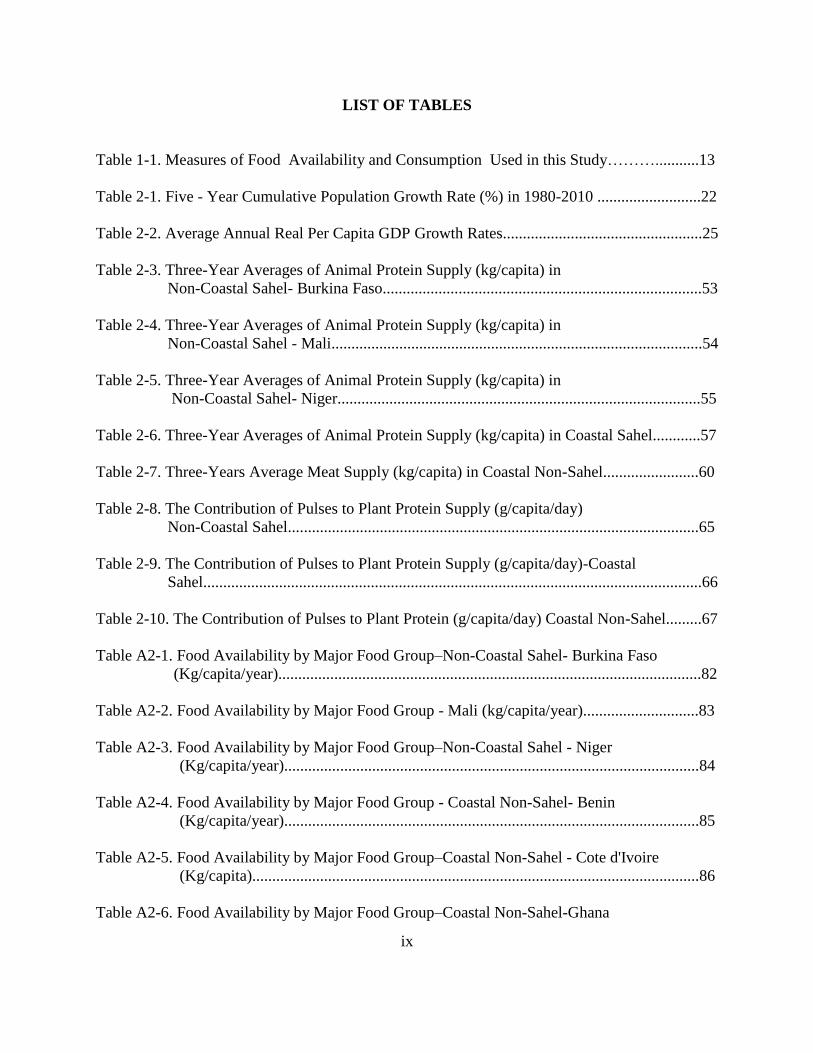
LIST OF TABLES
Table 1-1. Measures of Food Availability and Consumption Used in this Study………...........13
Table 2-1. Five - Year Cumulative Population Growth Rate (%) in 1980-2010 ..........................22
Table 2-2. Average Annual Real Per Capita GDP Growth Rates..................................................25
Table 2-3. Three-Year Averages of Animal Protein Supply (kg/capita) in
Non-Coastal Sahel- Burkina Faso................................................................................53
Table 2-4. Three-Year Averages of Animal Protein Supply (kg/capita) in
Non-Coastal Sahel - Mali.............................................................................................54
Table 2-5. Three-Year Averages of Animal Protein Supply (kg/capita) in
Non-Coastal Sahel- Niger...........................................................................................55
Table 2-6. Three-Year Averages of Animal Protein Supply (kg/capita) in Coastal Sahel............57
Table 2-7. Three-Years Average Meat Supply (kg/capita) in Coastal Non-Sahel........................60
Table 2-8. The Contribution of Pulses to Plant Protein Supply (g/capita/day)
Non-Coastal Sahel.......................................................................................................65
Table 2-9. The Contribution of Pulses to Plant Protein Supply (g/capita/day)-Coastal
Sahel.............................................................................................................................66
Table 2-10. The Contribution of Pulses to Plant Protein (g/capita/day) Coastal Non-Sahel.........67
Table A2-1. Food Availability by Major Food Group–Non-Coastal Sahel- Burkina Faso
(Kg/capita/year)..........................................................................................................82
Table A2-2. Food Availability by Major Food Group - Mali (kg/capita/year).............................83
Table A2-3. Food Availability by Major Food Group–Non-Coastal Sahel - Niger
(Kg/capita/year)........................................................................................................84
Table A2-4. Food Availability by Major Food Group - Coastal Non-Sahel- Benin
(Kg/capita/year)........................................................................................................85
Table A2-5. Food Availability by Major Food Group–Coastal Non-Sahel - Cote d'Ivoire
(Kg/capita)................................................................................................................86
Table A2-6. Food Availability by Major Food Group–Coastal Non-Sahel-Ghana
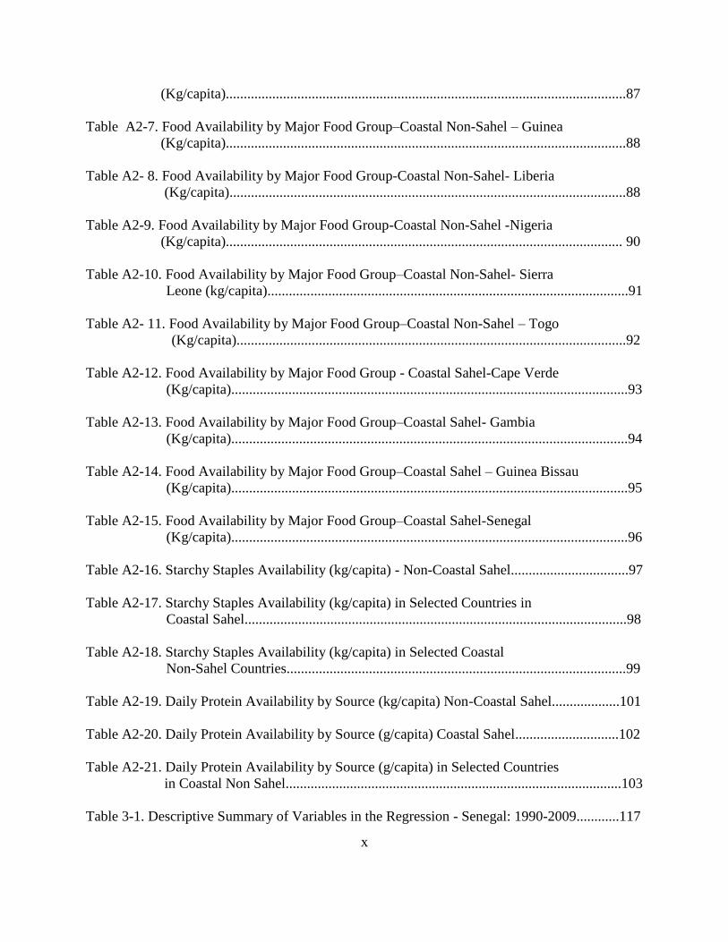
x
(Kg/capita)................................................................................................................87
Table A2-7. Food Availability by Major Food Group–Coastal Non-Sahel – Guinea
(Kg/capita)................................................................................................................88
Table A2- 8. Food Availability by Major Food Group-Coastal Non-Sahel- Liberia
(Kg/capita)...............................................................................................................88
Table A2-9. Food Availability by Major Food Group-Coastal Non-Sahel -Nigeria
(Kg/capita)............................................................................................................... 90
Table A2-10. Food Availability by Major Food Group–Coastal Non-Sahel- Sierra
Leone (kg/capita).....................................................................................................91
Table A2- 11. Food Availability by Major Food Group–Coastal Non-Sahel – Togo
(Kg/capita).............................................................................................................92
Table A2-12. Food Availability by Major Food Group - Coastal Sahel-Cape Verde
(Kg/capita)...............................................................................................................93
Table A2-13. Food Availability by Major Food Group–Coastal Sahel- Gambia
(Kg/capita)...............................................................................................................94
Table A2-14. Food Availability by Major Food Group–Coastal Sahel – Guinea Bissau
(Kg/capita)...............................................................................................................95
Table A2-15. Food Availability by Major Food Group–Coastal Sahel-Senegal
(Kg/capita)...............................................................................................................96
Table A2-16. Starchy Staples Availability (kg/capita) - Non-Coastal Sahel.................................97
Table A2-17. Starchy Staples Availability (kg/capita) in Selected Countries in
Coastal Sahel...........................................................................................................98
Table A2-18. Starchy Staples Availability (kg/capita) in Selected Coastal
Non-Sahel Countries...............................................................................................99
Table A2-19. Daily Protein Availability by Source (kg/capita) Non-Coastal Sahel...................101
Table A2-20. Daily Protein Availability by Source (g/capita) Coastal Sahel.............................102
Table A2-21. Daily Protein Availability by Source (g/capita) in Selected Countries
in Coastal Non Sahel..............................................................................................103
Table 3-1. Descriptive Summary of Variables in the Regression - Senegal: 1990-2009............117
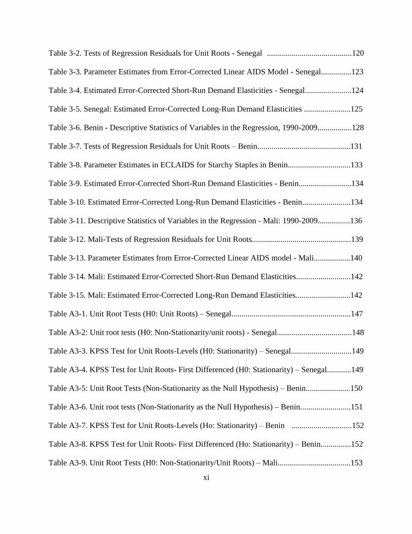
xi
Table 3-2. Tests of Regression Residuals for Unit Roots - Senegal ..........................................120
Table 3-3. Parameter Estimates from Error-Corrected Linear AIDS Model - Senegal...............123
Table 3-4. Estimated Error-Corrected Short-Run Demand Elasticities - Senegal.......................124
Table 3-5. Senegal: Estimated Error-Corrected Long-Run Demand Elasticities .......................125
Table 3-6. Benin - Descriptive Statistics of Variables in the Regression, 1990-2009.................128
Table 3-7. Tests of Regression Residuals for Unit Roots – Benin..............................................131
Table 3-8. Parameter Estimates in ECLAIDS for Starchy Staples in Benin...............................133
Table 3-9. Estimated Error-Corrected Short-Run Demand Elasticities - Benin..........................134
Table 3-10. Estimated Error-Corrected Long-Run Demand Elasticities - Benin........................134
Table 3-11. Descriptive Statistics of Variables in the Regression - Mali: 1990-2009................136
Table 3-12. Mali-Tests of Regression Residuals for Unit Roots.................................................139
Table 3-13. Parameter Estimates from Error-Corrected Linear AIDS model - Mali..................140
Table 3-14. Mali: Estimated Error-Corrected Short-Run Demand Elasticities...........................142
Table 3-15. Mali: Estimated Error-Corrected Long-Run Demand Elasticities...........................142
Table A3-1. Unit Root Tests (H0: Unit Roots) – Senegal...........................................................147
Table A3-2: Unit root tests (H0: Non-Stationarity/unit roots) - Senegal.....................................148
Table A3-3. KPSS Test for Unit Roots-Levels (H0: Stationarity) – Senegal..............................149
Table A3-4. KPSS Test for Unit Roots- First Differenced (H0: Stationarity) – Senegal............149
Table A3-5: Unit Root Tests (Non-Stationarity as the Null Hypothesis) – Benin......................150
Table A3-6. Unit root tests (Non-Stationarity as the Null Hypothesis) – Benin.........................151
Table A3-7. KPSS Test for Unit Roots-Levels (Ho: Stationarity) – Benin ..............................152
Table A3-8. KPSS Test for Unit Roots- First Differenced (Ho: Stationarity) – Benin...............152
Table A3-9. Unit Root Tests (H0: Non-Stationarity/Unit Roots) – Mali....................................153
xii
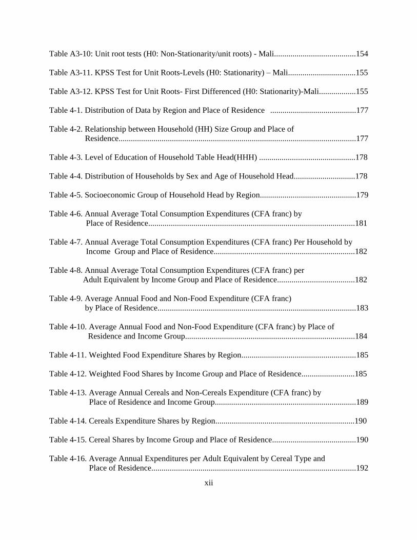
Table A3-10: Unit root tests (H0: Non-Stationarity/unit roots) - Mali........................................154
Table A3-11. KPSS Test for Unit Roots-Levels (H0: Stationarity) – Mali.................................155
Table A3-12. KPSS Test for Unit Roots- First Differenced (H0: Stationarity)-Mali..................155
Table 4-1. Distribution of Data by Region and Place of Residence ..........................................177
Table 4-2. Relationship between Household (HH) Size Group and Place of
Residence....................................................................................................................177
Table 4-3. Level of Education of Household Table Head(HHH) ...............................................178
Table 4-4. Distribution of Households by Sex and Age of Household Head..............................178
Table 4-5. Socioeconomic Group of Household Head by Region...............................................179
Table 4-6. Annual Average Total Consumption Expenditures (CFA franc) by
Place of Residence.....................................................................................................181
Table 4-7. Annual Average Total Consumption Expenditures (CFA franc) Per Household by
Income Group and Place of Residence.....................................................................182
Table 4-8. Annual Average Total Consumption Expenditures (CFA franc) per
Adult Equivalent by Income Group and Place of Residence......................................182
Table 4-9. Average Annual Food and Non-Food Expenditure (CFA franc)
by Place of Residence.................................................................................................183
Table 4-10. Average Annual Food and Non-Food Expenditure (CFA franc) by Place of
Residence and Income Group...................................................................................184
Table 4-11. Weighted Food Expenditure Shares by Region........................................................185
Table 4-12. Weighted Food Shares by Income Group and Place of Residence..........................185
Table 4-13. Average Annual Cereals and Non-Cereals Expenditure (CFA franc) by
Place of Residence and Income Group.....................................................................189
Table 4-14. Cereals Expenditure Shares by Region....................................................................190
Table 4-15. Cereal Shares by Income Group and Place of Residence.........................................190
Table 4-16. Average Annual Expenditures per Adult Equivalent by Cereal Type and
Place of Residence....................................................................................................192
xiii
Table 4-17. Average Annual Expenditures (CFA franc/AE) by Cereal Type and
Place of Residence....................................................................................................193
Table 4-18. Average Annual Expenditures (CFA franc/AE) by Cereal Type, by
Income Group and Place of Residence.....................................................................194
Table 4-19. Shares in Cereal Budget by Cereal Type, Place of Residence and
Income Group ......................................................................................................196
Table 4-20. Estimated Reduced Forms for Cereals Expenditure and Cereal
Expenditure Squared................................................................................................200
Table 4-21. Results of the Test for the Endogeneity of Expenditure...........................................201
Table 4-22. Tests for Nonlinearity of the Demand System Based on Statistical Significance of
the Coefficient of the Price Times Expenditure-Squared Terms.............................202
Table 4-23. Cereals Expenditure Elasticities by Place of Residence and Income Group............206
Table 4-24. Cereals Own-Price Elasticities - By Place of Residence and Income Group...........209
Table 4-25. Compensated Cross-Price Elasticities - By Place of Residence...............................211
Table 4-26. Urban Compensated Cross-Price Elasticities by Income Group..............................213
Table 4-27. Rural Compensated Cross-Price Elasticities by Income Group...............................215
Table A4-1. Structure of ELIM-2006 data................................................................................. 220
Table A4-2. Number of Zero Expenditures by Place of Residence-Considering Expenditure
on All Modes of Acquisition.................................................................................. 226
Table A4-3. Zero-Expenditure by Mode of Acquisition.............................................................226
Table A4-4. Estimated Parameters of the Censored QUAIDS model for Cereals Demand- by
Place of Residence – Total Cereals Expenditure......................................................227
Table A4-5. Estimated Elasticities of the Censored QUAIDS model for Cereals Demand
by Place of Residence- Total Cereals Expenditures................................................229
Table A4-6. Estimated Elasticities of the Censored QUAIDS model for Cereals Demand
by Urban- Income Group- Total Cereals Expenditures............................................231
Table A4-7. Estimated Elasticities of the Censored QUAIDS model for Cereals Demand
by Rural- Income Group - Total Cereals Expenditures...........................................233
Table A4-8. Estimated Parameters of the Censored QUAIDS model for Cereals Demand
xiv
by Place of Residence – Only Purchased Cereals Expenditure..............................235
Table A4-9. Estimated Elasticities of the Censored QUAIDS model for Cereals Demand
by Place of Residence- Only Purchased Cereals Expenditures..............................238
Table A4-10. Estimated Elasticities of the Censored QUAIDS model for Cereals Demand by
Urban- Income Group- Only Purchased Cereals Expenditures.............................240
Table A4-11. Estimated Elasticities of the Censored QUAIDS model for Cereals Demand by
Rural- Income Group- Only Purchased Cereals Expenditures..............................242
Table 5-1. Average Consumer Price Changes Compared to 2006 (%).......................................250
Table 5-2. Compensating Variation of Cereals Price Changes by Place of Residence
(% of Total Cereals Expenditures).............................................................................251
Table 5-3. Magnitude of Welfare Loss Implied by Cereals Price Changes by
Place of Residence.....................................................................................................253
Table 5-4. Compensating Variation of Cereals Price Changes by Place of Residence
and Income Group (% of total Cereals Expenditures)...............................................254
Table 5-5. Magnitude of Welfare Loss Implied by Cereals Price Changes by Place
of Residence and per Capita Income Group................................................................256
Table 5-6. Compensating Variation Implied by Rice Price Changes by Place of
Residence (%)............................................................................................................257
Table 5-7. Magnitude of Welfare Loss Implied by Rice Price Changes by Place of
Residence...................................................................................................................258
Table 5-8. Welfare Effects of Rice Price Increases by Place of Residence and
Income Group (%).....................................................................................................259
Table 5-9. Magnitude of Welfare Loss Implied by Rice Price Changes by Place of
Residence and per Capita Income Group..................................................................260
xv
LIST OF FIGURES
Figure 1-1. Map of West Africa......................................................................................................2
Figure 1-2. Annual Food Price Index (2002-2004=100).................................................................3
Figure 2-1. Urban Population Shares (%) - West Africa (1980-2010) ...................................... ...23
Figure 2-2. Daily Energy Availability (kcal/capita/day) - Non-Coastal Sahel…………………..29
Figure 2-3. Daily Energy Availability (kcal/capita/day) - Coastal Sahel………………………..29
Figure 2-4. Daily Energy Availability (kcal/capita/day) - Coastal Non-Sahel…………………..30
Figure 2-5. Major Starchy Staples Availability - Mali (kg/capita/year) ………………………...37
Figure 2-6. Major Starchy Staples Availability - Cape Verde (kg/capita/year) ………………...38
Figure 2-7. Major Starchy Staples Availability - Senegal (kg/capita/year)……………………...39
Figure 2-8. Major Starchy Staples Availability - Ghana (kg/capita/year)……………………….42
Figure 2-9. Major Starchy Staples Availability - Nigeria (kg/capita/year)……………………...43
Figure 2-10. Protein Availability (g/capita/day) Non-Coastal Sahel……………………………45
Figure 2-11. Protein Availability (g/capita/day)-Coastal Sahel…………………………………45
Figure 2-12. Protein Availability (g/capita/day)-Coastal Non-Sahel……………………………46
Figure 2-13. Animal Protein Availability (g/capita/day) Non-Coastal Sahel……………………47
Figure 2-14. Animal Protein Availability (g/capita/day) Coastal Sahel…………………………48
Figure 2-15. Animal Protein Availability (g/capita/day) Coastal Non-Sahel……………………50
Figure 2-16. Fat Availability (g/capita/day) Non-Coastal Sahel...………………………………69
Figure 2-17. Fat Availability (g/capita/day) Coastal Sahel……………………………………...70
Figure 2-18. Fat Availability (g/capita/day) Coastal Non-Sahel………………………………...70
Figure 2-19. Daily Caloric Share (%) by Macronutrients - Non-Coastal Sahel…………………74
xvi
Figure 2-20. Daily Caloric Share (%) by Macronutrients - Coastal Sahel………………………75
Figure 2-21. Daily Caloric Share (%) by Macronutrients - Coastal Non-Sahel…………………76
Figure 3-1. Shares in Cereals Budget - Senegal: 1990-2009 ...................................................... 118
Figure 3-2. Natural Logarithm of Deflated Cereals Prices - Senegal: 1990-2009 ...................... 118
Figure 3-3. Shares in Starchy Staples Budget - Benin: 1990-2009 ............................................ 129
Figure 3-4. Logarithm Transformed Deflated Starchy Staples Prices - Benin: 1990-2009 ........ 129
Figure 3-5. Shares in Cereals Budget - Mali: 1990-2009 ........................................................... 136
Figure 3-6. Logarithm Transformed Deflated Cereals Prices - Mali: 1990-2009 ...................... 137
Figure 4-1. Food Expenditures per Capita and Total Household Consumption Expenditures
per Capita (CFA franc)……………………………………………………….........186
Figure 4-2. Food Expenditure Shares and Total Household Consumption Expenditures .......... 187
Figure 4-3. Total Household Food Expenditure and the Share of Cereals in Food Budget ....... 191
Figure 4-4. Cereals Expenditures (CFA franc/AE) by Income Group and Place of Residence..195
Figure 4-5. Shares in Cereal Budget by Cereal Type Place of Residence and Income Group ... 196
xvii
KEY TO ABBREVIATIONS
ADF–Augmented Dickey-Fuller
AIDS–Almost Ideal Demand System
CDF–Standard Normal Cumulative Distribution Functions
CFA franc–Common Currency for West African States
CV–Proportional Compensating Variation
DEA–Daily Energy Availability
ECLAIDS–Error Corrected Linearized Almost Ideal Demand System
ECOWAS– Economic Community of West African States
ELIM–Enquête Légère Intégrée Auprès des Ménages
FAO–Food and Agricultural Organization of the United Nations
FBS–Food Balance Sheet
GDP–Gross Domestic Product
HBS–Household Budget Survey
HH–Household
HHH–Household Head
IV–Instrumental Variable
KPSS–Kwiatkowski–Phillips–Schmidt–Shin tests
MPC–Marginal Propensity to Consume
OLS–Ordinary Least Squares
OMA–Observatoire du Marché Agricole
PDF–Standard Normal Probability Density Function
xviii
PP–Phillips-Perron
QUAIDS–Quadratic Almost Ideal Demand System
R&T–Roots and Tubers
SAP–Structural Adjustment Programs
WA–West Africa
1
CHAPTER 1. INTRODUCTION
1.1. Issue and Background
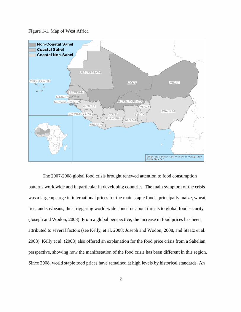
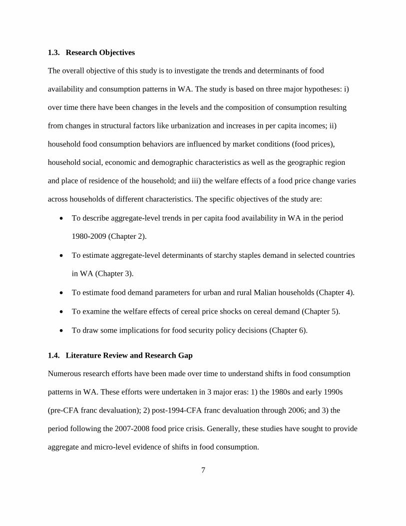
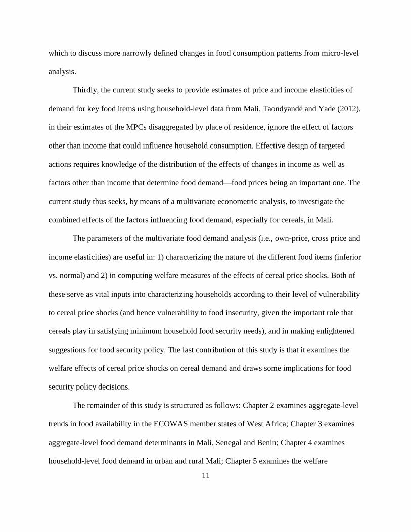
The region of West Africa (WA) includes 16 countries: Benin, Burkina Faso, Cape Verde, Cote
d’Ivoire, Gambia, Ghana, Guinea, Guinea Bissau, Liberia, Mali, Mauritania, Niger, Nigeria,
Senegal, Sierra Leone, and Togo. A map of WA is available in Figure 1-1. With the exception of
Mauritania, all of these countries are members of the Economic Community of West African
States (ECOWAS). This study focuses on ECOWAS member countries since ECOWAS has a
major role in defining agricultural policy for the region.
WA has undergone rapid changes in its social and economic environment during the last
25 years, resulting in shifts in food consumption patterns. Some of these changes include
urbanization, growth in per capita incomes, population growth, in a few countries a demographic
transition towards smaller family sizes, migration within the zone towards the coastal states, and
the adoption of more western lifestyles (Lopriore and Muehlhof, 2003; Satterthwaite et. al,
2010). In addition to the aforementioned structural factors, the region has undergone policy shifts
that constituted major changes in the conditions that determine demand. Examples of these
include the Structural Adjustment Programs (SAP) and the 1994 CFA franc devaluation that
brought about changes in relative cereal prices, thereby increasing the domestic price of rice
relative to that of the local coarse grains (Camara, 2004).
2
Figure 1-1. Map of West Africa
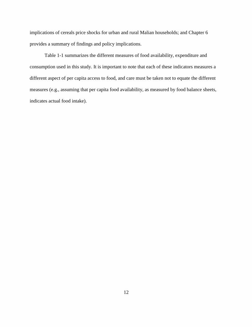
The 2007-2008 global food crisis brought renewed attention to food consumption
patterns worldwide and in particular in developing countries. The main symptom of the crisis
was a large upsurge in international prices for the main staple foods, principally maize, wheat,
rice, and soybeans, thus triggering world-wide concerns about threats to global food security
(Joseph and Wodon, 2008). From a global perspective, the increase in food prices has been
attributed to several factors (see Kelly, et al. 2008; Joseph and Wodon, 2008, and Staatz et al.
2008). Kelly et al. (2008) also offered an explanation for the food price crisis from a Sahelian
perspective, showing how the manifestation of the food crisis has been different in this region.
Since 2008, world staple food prices have remained at high levels by historical standards. An
3
examination of the Food and Agricultural Organization (FAO)’s food price index (see Figure
1.2), a measure of the change in international prices of a basket of food commodities, shows that
in 2011 the index rose above its 2008 peak. The index dropped in 2012 (nominal terms) but still
remained generally higher than its 2008 level.1
Figure 1-2. Annual Food Price Index (2002-2004=100)
Source: Author’s computation using FAO’s food price index.
The circumstances of the global food crisis in WA, which previously relied on cheap
food imports for a substantial part of its staple food supply, have been unique.2 As observed by
1FAO, Food Price Index: http://www.fao.org/worldfoodsituation/FoodPricesIndex/en/. 2 The deregulation of domestic food markets and the liberalization of agriculture experienced as
part of the SAP in the region forced most of West African nations into competition in the world
food markets with developed country producers that produced at lower costs and sold at lower
prices, sometimes due to substantial subsidies provided to their farmers and exporters.
0
50
100
150
200
250
1990
1991
1992
1993
1994
1995
1996
1997
1998
1999
2000
2001
2002
2003
2004
2005
2006
2007
2008
2009
2010
2011
2012
Real
Nominal
4
Staatz et al. (2008), trade bans and high international food prices pushed many West African
countries away from their historical reliance on regional and international trade as a key
component of their food security strategies, thereby leading many governments to conclude that
the risks were very high in depending on the international market for staples. Kelly et al. (2008)
also observed that in the Sahel region, the impact of the food price crisis on household
consumption has been differentiated according to each country’s food consumption profile and
food supply. However, in spite of production shortfalls in some countries, there is a strong
potential for production stability at the regional level (Kelly et al. 2008).
1.2. Problem Statement
Food demand is determined by factors at the national (aggregate), the intermediate, and the
household (micro) level. Aggregate-level determinants of food consumption include population,
urbanization, per capita incomes and overall changes in lifestyle. Intermediate-level determinants
include factors such as cultural changes that affect changes in tastes and preferences. Household-
level factors include households’ economic and socio-demographic characteristics such as
household composition (size, age and sex), income level and geographic location. Households
therefore differ among themselves in food consumption behavior and, in particular, in their
response to changes in market conditions. The analysis of food consumption provides
information on: 1) food demand elasticities (own-price, cross-price and income elasticities); 2)
differences in demand patterns by urban/rural location, by geographical region, by socio-
economic group and across households of different demographic composition. Such an analysis
also provides parameters needed to understand the adjustments of consumption in the macro
food economy.
5
Knowledge of food demand parameters and of how consumption patterns have changed
over time is critical for informed policy making. However, in WA, information on food demand
parameters is limited, thus restricting policymakers’ ability to make sound food policy decisions.
One ultimate goal of the analysis of food consumption patterns is to improve the efficiency of
government interventions by providing policymakers, for example, with suggestions for the
design of safety nets compatible with targeting people based on the nature and extent of food
insecurity. According to Kelly et al. (2008), the greatest challenge in the design of policies and
programs that will help households cope with the rising food prices is the identification of
vulnerable groups so that targeting would be towards the neediest and not towards the most vocal
constituencies.
A major concern has been that the price hikes for internationally traded food products are
being transmitted to local cereals such as millet, maize, and sorghum due to substitutions in
production and consumption. For instance, Joseph and Wodon (2008) observed that just as the
prices of imported food products–rice and wheat—have been increasing, the prices of other
foods that might be thought of as substitutes (millet, sorghum and maize) in Mali have also
increased recently. They attributed this change to increases in cost of production and alternate
demand for grains (animal feed). Diallo et al. (2010) found that 33% of price increases have been
transmitted from international to local markets in WA, mainly for rice and wheat. However, the
impact varies: countries with coastline (Guinea, Ivory Coast and Senegal) are more affected than
landlocked ones (Mali, Niger and Burkina (Diallo et al. 2010). This difference is likely a result
of differences in the cost of inland transport, since in absolute terms the transmission may be
similar across countries. Food price transmission from international to African markets also
differs across commodities (Minot, 2010).
6
Historically, cereals have represented a large share of total household consumption in the
Sahel. Staatz et al. (2008) observed a growing demand for cereals in WA and attribute this to
population growth, urbanization and consumers’ demand for more products (including livestock
products) that require cereals as intermediate inputs as income increases. Given the importance
of grains in the West African food basket, a major source of concern in the context of rising food
prices is the possible reduction of consumption levels whereby households may be forced to
reduce both their food consumption in response to the price surge and other longer-term non-
food expenditures in order to meet basic needs. Camara (2004) found that Bamako households
engage in food consumption smoothing from seasonal shocks in real incomes at the expense of
non-food commodities, of non-staple foods, and through significant substitutions among and
between broad expenditure items such as health and education. Data limitations prevent an actual
examination of food consumption behavior following the 2007-08 food crisis. However, using
Mali’s 2006 household budget survey (HBS) data as a base year, this study examines the
possible effects of cereal price shocks on household welfare for different segments of the
population.
Changing food consumption patterns also have implications for agricultural market
development, currently a priority for WA’s development agenda. With urbanization and the
growing urban middle class in WA, understanding how these patterns have changed (in level and
diversity), whether new food groups are emerging as important sources of household food energy
consumption and whether the traditional cereal habits persist, will help identify opportunities and
challenges for the development of agricultural value chains to meet the growing effective
demand. The findings of this study will contribute to the knowledge base and policy dialogue at
regional and national levels on key policy issues concerning the evolution of agri-food systems.
7
1.3. Research Objectives
The overall objective of this study is to investigate the trends and determinants of food
availability and consumption patterns in WA. The study is based on three major hypotheses: i)
over time there have been changes in the levels and the composition of consumption resulting
from changes in structural factors like urbanization and increases in per capita incomes; ii)
household food consumption behaviors are influenced by market conditions (food prices),
household social, economic and demographic characteristics as well as the geographic region
and place of residence of the household; and iii) the welfare effects of a food price change varies
across households of different characteristics. The specific objectives of the study are:
To describe aggregate-level trends in per capita food availability in WA in the period
1980-2009 (Chapter 2).
To estimate aggregate-level determinants of starchy staples demand in selected countries
in WA (Chapter 3).
To estimate food demand parameters for urban and rural Malian households (Chapter 4).
To examine the welfare effects of cereal price shocks on cereal demand (Chapter 5).
To draw some implications for food security policy decisions (Chapter 6).
1.4. Literature Review and Research Gap
Numerous research efforts have been made over time to understand shifts in food consumption
patterns in WA. These efforts were undertaken in 3 major eras: 1) the 1980s and early 1990s
(pre-CFA franc devaluation); 2) post-1994-CFA franc devaluation through 2006; and 3) the
period following the 2007-2008 food price crisis. Generally, these studies have sought to provide
aggregate and micro-level evidence of shifts in food consumption.
8
The 1980s and early 1990s was a period characterized by heavy reliance on imports for
household food grain needs. The heavy reliance was attributed to the declining competitiveness
of WA food production relative to other producers in the world. A major research question
during the 1980s and 1990s was whether the high consumption of imported rice and wheat was
caused by relatively low rice and wheat prices. A key finding during this period was that the
consumption of imported grains (especially rice) was not driven by relative cereal prices
(Reardon et al. 19883 ; Delgado, 19894; and Rogers and Lowdermilk, 19915). According to
Delgado and Reardon (1992), the switch to rice consumption in the West African Semi-Arid
Tropics appeared to be driven more by structural factors than by shorter-run factors such as
harvest shortfalls or price dips. They concluded that rice and wheat prices would have to increase
very substantially over those of millet and sorghum before encouraging shifts in consumption
back to coarse grains.
The 1994 devaluation of the common currency of many West African countries
represented a major policy shift that changed the conditions that determine demand. An intended
consequence of the devaluation was to raise the costs of all tradable goods relative to non-
tradable goods and reverse the trend in cereal demand from imported to locally produced grains.
Evidence based on post-devaluation studies suggests relatively low rates of substitution of coarse
grains for rice in urban centers of the Sahel. Diagana et al. (1999) studied urban WA
consumption patterns (Mali, Burkina Faso, Senegal and Cote d’Ivoire), and they found that the
general pattern was a reduction in cereal intake (actual quantity consumed in kilograms), but the
3 Using data household-level data from urban Burkina Faso. 4 Using country level data for Burkina Faso, Cote d’Ivoire, Mali, Niger and Senegal. 5 Using household-level data from urban Mali.
9
expected shift from imported rice to local coarse grains as a result of price hikes for imported
cereals did not occur in these countries, with the exception of Burkina Faso. The lack of such a
shift was attributed to the lackluster supply response of the coarse grain sectors and the resilience
of rice demand based on its convenience of processing and preparation for the urban consumer.
Camara (2004) investigated the impact of seasonal changes in real incomes and relative prices on
households’ consumption patterns in Bamako, Mali. She found that Bamako households’
consumption patterns are responsive to changes in real incomes and relative prices in any given
season and that there are seasonal changes in income and price responsiveness for all
commodities in the three demand models she estimated.
Evidence on food consumption patterns in WA following the 2007-2008 food price crisis
is relatively thin. Joseph and Wodon (2008) examined patterns of food consumption in Mali to
understand differences across households groups as defined by their level of consumption and, in
particular, the differential impact on poverty of higher food prices. They assumed that the cost of
an increase in the price of a food commodity for a household translates into an equivalent
reduction of its consumption in real terms (unit-own price elasticity). They neither estimated nor
took into account the own-price or cross-price elasticities of demand, which may lead to
substitution effects and thereby help offset part of the negative effect of higher prices for certain
food items. They assumed constant relative prices and argued that the substitution of millet,
sorghum, and maize for rice and wheat is likely to be low in any case, due to the fact that all
these products are important in the diet of the population and that the prices of the various food
items seem to increase in parallel at least in the medium term (so that it is not clear that
households can offset the loss in purchasing power associated with the price increase by shifting
10
to other foods). They admitted the roughness of their approach and the possibility of slightly
overestimating the impact on poverty of changes in prices.
Taondyandé and Yade (2012) examined, using descriptive and econometric approaches,
how food consumption patterns had changed over time with increased per capita incomes and the
growth in urban population. They also examined how food demand prospects would likely
change as a result of changes in per capita income and by place of residence. Specifically, they
estimated the additional demand for food (marginal propensity to consume, MPC) from an
increase in per capita income as well as income elasticities. However, they do not control for
price variation across the sample.
1.5. Research Contributions
The aim of the current study is to build on the Taondyandé and Yade (2012) study in four
important ways. Firstly, this study examines aggregate (national) level trends in food availability
patterns from national official statistics (as reported through FAO’s FBS). In particular, this
analysis will help us identify major contributors to food availability as well as identify any new
food groups emerging as important contributors to food availability in the region.
Secondly, the study examines aggregate-level determinants of starchy staples demand in
selected countries using a theoretically appropriate framework of analysis. In particular,
aggregate-level demand parameters are obtained by estimating, separately for each of the
countries considered, the impact of the structural variables and prices on startchy staples
expenditures. Aggregate-level food demand analysis provides an understanding of the linkages
between macroeconomic performance and food consumption and, through the food marketing
sector, incentives for agricultural production. Overall, such an analysis provides a context in
11
which to discuss more narrowly defined changes in food consumption patterns from micro-level
analysis.
Thirdly, the current study seeks to provide estimates of price and income elasticities of
demand for key food items using household-level data from Mali. Taondyandé and Yade (2012),
in their estimates of the MPCs disaggregated by place of residence, ignore the effect of factors
other than income that could influence household consumption. Effective design of targeted
actions requires knowledge of the distribution of the effects of changes in income as well as
factors other than income that determine food demand—food prices being an important one. The
current study thus seeks, by means of a multivariate econometric analysis, to investigate the
combined effects of the factors influencing food demand, especially for cereals, in Mali.
The parameters of the multivariate food demand analysis (i.e., own-price, cross price and
income elasticities) are useful in: 1) characterizing the nature of the different food items (inferior
vs. normal) and 2) in computing welfare measures of the effects of cereal price shocks. Both of
these serve as vital inputs into characterizing households according to their level of vulnerability
to cereal price shocks (and hence vulnerability to food insecurity, given the important role that
cereals play in satisfying minimum household food security needs), and in making enlightened
suggestions for food security policy. The last contribution of this study is that it examines the
welfare effects of cereal price shocks on cereal demand and draws some implications for food
security policy decisions.
The remainder of this study is structured as follows: Chapter 2 examines aggregate-level
trends in food availability in the ECOWAS member states of West Africa; Chapter 3 examines
aggregate-level food demand determinants in Mali, Senegal and Benin; Chapter 4 examines
household-level food demand in urban and rural Mali; Chapter 5 examines the welfare
12
implications of cereals price shocks for urban and rural Malian households; and Chapter 6
provides a summary of findings and policy implications.
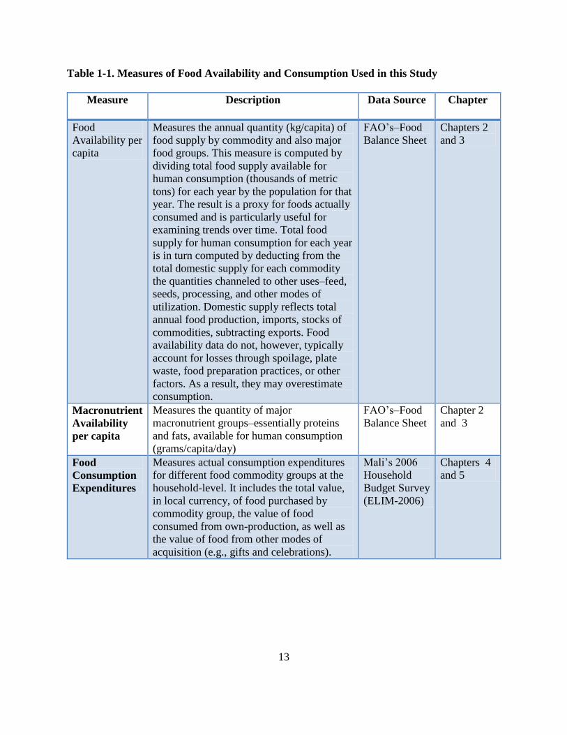
Table 1-1 summarizes the different measures of food availability, expenditure and
consumption used in this study. It is important to note that each of these indicators measures a
different aspect of per capita access to food, and care must be taken not to equate the different
measures (e.g., assuming that per capita food availability, as measured by food balance sheets,
indicates actual food intake).
13
Table 1-1. Measures of Food Availability and Consumption Used in this Study
Measure Description Data Source Chapter
Food
Availability per
capita
Measures the annual quantity (kg/capita) of
food supply by commodity and also major
food groups. This measure is computed by
dividing total food supply available for
human consumption (thousands of metric
tons) for each year by the population for that
year. The result is a proxy for foods actually
consumed and is particularly useful for
examining trends over time. Total food
supply for human consumption for each year
is in turn computed by deducting from the
total domestic supply for each commodity
the quantities channeled to other uses–feed,
seeds, processing, and other modes of
utilization. Domestic supply reflects total
annual food production, imports, stocks of
commodities, subtracting exports. Food
availability data do not, however, typically
account for losses through spoilage, plate
waste, food preparation practices, or other
factors. As a result, they may overestimate
consumption.
FAO’s–Food
Balance Sheet
Chapters 2
and 3
Macronutrient
Availability
per capita
Measures the quantity of major
macronutrient groups–essentially proteins
and fats, available for human consumption
(grams/capita/day)
FAO’s–Food
Balance Sheet
Chapter 2
and 3
Food
Consumption
Expenditures
Measures actual consumption expenditures
for different food commodity groups at the
household-level. It includes the total value,
in local currency, of food purchased by
commodity group, the value of food
consumed from own-production, as well as
the value of food from other modes of
acquisition (e.g., gifts and celebrations).
Mali’s 2006
Household
Budget Survey
(ELIM-2006)
Chapters 4
and 5
14
CHAPTER 2. TRENDS IN PER CAPITA FOOD AVAILABILITY IN WEST AFRICA
2.1. Introduction
Understanding how patterns of per capita food availabilty have changed with changes in
urbanization, per capita incomes, population growth, migration within the zone towards the
coastal states, and the adoption of more western lifestyles is necessary in identifying
opportunities and challenges for the development of agricultural value chains to meet the
growing effective demand in the region.
Lopriore and Muehlhoff (2003) documented the most recent evidence (prior to this study)
on aggregate per capita food availability patterns in WA from food balance sheets (FBS). They
analyzed trends in dietary energy supply and also in the quality and diversity of per capita food
supplies. However, their analysis covers only up to the year 2001. This chapter expands and
updates the Lopriore and Muehlhoff analysis by providing a more comprehensive and up-to-date
picture of the trends in per capita food availability in WA, discussing what is happening in the
“big drivers” of change in the region (e.g., Nigeria and Ghana) as well as analyzing shifts in per
capita food availability in the context of the social, economic and political changes that have
occurred in the region.
2.2. Objectives and Hypotheses
This chapter investigates from national official statistics (as reported through FAO’s FBS)
aggregate (national) trends in per capita food availability in WA in the period 1980-20096. The
analysis is carried out on the 15 ECOWAS member states, and it will help identify major
6 Most recent FAO food balance sheet data are of 2009.
15
contributors to the national food supply (in terms of the major food commodities) as well as new
food groups emerging as important contributors to the diet. The analysis is intended to test the
following hypotheses:
Hypothesis 2.1: As a result of rising per capita incomes, there has been an increase in the level
of per capita calorie availability in the past 30 years.
Hypothesis 2.2: In the past 30 years, there has been a diversification in the composition of food
supply, whereby new food groups (e.g., roots and tubers in the non-coastal Sahelian West
African countries and maize in the landlocked countries) are emerging as important contributors
to the daily caloric supply.
Hypothesis 2.3: The contribution of animal protein to total daily protein supply has increased
over time as per capita incomes have increased.
Hypothesis 2.4: Based on FAO’s recommended daily allowances of various nutrients for a
balanced diet, the per capita food supply has become more balanced in terms of macronutrient
composition.
2.3. Data and Reliability of Food Balance Sheet Consumption Estimates
Data for the period 1980-2009 per country obtained from FAO’s FBS are used for the analysis of
aggregate-level trends in per capita food availability. The FBS calculate domestic food supply as
production plus imports, plus stocks, and less exports. Not all domestic supply is available as
food for human consumption due to other uses – feed, seeds, processing and other modes of
utilization. These are deducted from the total, and the remaining supply for food use is converted
into estimated per capita availability by dividing the total by an estimate of the country’s
16
population. The physical amounts of food available per person are then converted into per capita
availability of calories, protein and fat using a food composition table.
The reliability of the FBS as a source of national average per capita food availability
estimates has been questioned. For instance, Farnsworth (1961) examined the statistical
shortcomings in the construction of food balances and argued that the FBS figures on per capita
availability depend on the accuracy of the production, stocks, and population figures, all of
which are subject to varying degrees of error across countries. She noted that the cassava
production figures deserve special attention, because they illustrate a peculiarly difficult balance
sheet construction problem encountered in many African countries. Unlike practically all other
staple foods, mature cassava can be harvested at any time over a period of years. Moreover, since
cassava usua1ly ranks as a non-preferred food, and since it is often planted for price specu1ation
and as a "hungry season" reserve, large quantities are never harvested but remain on land
abandoned to bush fallow. Hence, if cassava production is estimated by applying data on
sampled yields per acre to the total acreage under cassava, the result is inevitably an inflated
"potential production" figure, rather than an indication of the crop harvested in a single year.
Farnsworth acknowledged that some allowances were made for this peculiar “cassava estimation
problem”, as well as for other balance sheet uncertainties, and she presents some other caveats
on the using FBS data to estimate actual per capita food consumption. These include:
The FBS estimates measure "net availability" or "net supplies" of food at the so-called
"retail level," and this includes not only food delivered to retail outlets and restaurants,
but also food bartered, given away, or immediately eaten after harvesting.
17
The estimates represent the broad pattern of total food supplies, and while the estimates
indicate important calorie contributors, the data afford no firm basis for determining
which of the most important food groups furnishes the largest (or smallest) number of
food calories.
The estimates show whether the hypothetical "average person" of a given country
customarily consumes much or very little meat or milk as compared with “average
persons" in other countries; whether the specified country depends very heavily or very
little on the typical "cheap foods"–cereals and major starchy roots and tubers; whether
wheat, rice or some specified cheaper grain is the dominant cereal; and what kind of
starchy roots and tubers are most common.
For many low-income countries, the national average pattern of consumption represents a
composite of several distinctly different types of diets consumed by different subgroups
of the population (e.g., regional subgroups in Nigeria) and as a result may not yield the
best information on subgroup diets (available from good dietary surveys that are
representative samples of the population, with complete food coverage and taking
adequate account of varying seasonal patterns of consumption).
The estimates often reflect the underestimation or overestimation of agricultural
production –a characteristic of the agricultural statistics of practically all countries. The
underestimation could be from incomplete coverage (of crop areas or crops) or tax-
related purposes (particularly in low-income countries where taxes are often tied directly
or indirectly to farm output). Such crop reporting deficiencies are much greater for
subsistence crops than for commercial crops, and greater for minor than major crops, and
greater for secondary successive and mixed crops than for single primary crops.
18
Overestimation occurs in some countries, when (1) pre-harvest sampling methods are
employed without appropriate adjustment for later losses, and (2) government officials
fabricate or "adjust" yield and production figures primarily for the purpose of impressing
either the voting public or their own superiors.
The estimates are at their worst when constructed for individual years and accepted as
evidence of year-to-year changes in consumption. Only the largest indicated annual
changes, say 20 per cent or more, can be relied on as reflections of actual variations in
food consumption in most countries, and even these only as indicators of the direction,
not the magnitude of change.
The estimates at the “retail level" are not the same as the estimated nutrient intake due to
losses and waste. Furthermore, nutrient losses and waste beyond the “retail level" vary
markedly from country to country, from commodity to commodity7, from year to year
(depending mainly on weather conditions and crop quality), and from times of food
shortage to times of plenty. Farnsworth acknowledged that the FAO estimators employ a
uniform 15 per cent allowance for such losses.
Farnsworth wrote her piece of work more than half a century ago. While some of the concerns
about the manner in which FBS are constructed may still be valid, it is also most likely true that
national agricultural statistics have improved substantially over time in the estimation of food
availability. Nonetheless, her caveats about FBS data still need to be borne in mind. For
7 For example in tropical countries heavily dependent on root crops, plantains, and maize, not
only do such foods deteriorate rapidly after harvest in hot, moist climates, but some of the less-
desired staples, like cassava, may be so amply available that they are wastefully prepared for
consumption in producing areas.
19
example, a question can be raised about the extent to which any apparent diversification of the
food supply over time shown by the FBS reflects real diversification versus just an improvement
in the ability of national agricultural statistics to capture production of secondary crops
(particularly non-cereal production). Notwithstanding the criticisms of food balance sheets,
Timmer et al., (1983) argued that the analysis of FBS is the starting point for most food policy
analysis at the country level. Lopriore and Muehlhoff (2003) also observed that although the
analysis of food supply data derived from FAO’s FBS do not provide information on
consumption patterns and tend to overestimate intakes, it can be used to describe the trends in the
structure of a national diet in terms of the major food commodities. Smith and Haddad (2000)
also argued that per capita daily energy availability (DEA) from the FAO’s FBS is one of the
main indicators of national food availability. The authors provide empirical evidence suggesting
that there is a strong correlation between this per capita DEA and more individual-based
indicators of food security (e.g., anthropometric indicators of children’s nutritional status). In
particular, Smith and Haddad (2000) show that national caloric availability was responsible for
more than a quarter of reductions in child malnutrition in developing countries over the period
1970-95.
20
2.4. Methodological Approach
Food supply data from the FAO’s FBS is used to describe aggregate trends in the structure of per
capita food availability, by country, in terms of the major food commodities. The FAO’s FBS
shows national and per capita quantities of food available for human consumption for almost all
food commodities and all countries. The FBS also shows data on per capita food energy
availability as well as the availability of individual macronutrient groups (proteins and fats). The
analysis of protein availability by source and fat supply helps to better understand changes in the
quality of the food available in terms of major macronutrients. With data on per capita
availability of individual macronutrients and information on the nutrient conversions for each
macronutrient8, the caloric (or energy) contribution of proteins and fats are calculated. According
to FAO (2000), the healthy range of macronutrient intake (what FAO calls “a balanced diet”),
expressed as a percent of total energy, can be broad: 55-75% from carbohydrates, 15-35% from
fats and 10-15% from proteins.
For these key variables, three-year averages are computed to facilitate comparison. In
most cases, the results are presented by specific sub-regions in ECOWAS-WA. These include
the Non-Coastal Sahel (Mali, Burkina Faso and Niger); the Coastal Sahel (Cape Verde, Gambia,
Guinea Bissau, Senegal); and the Coastal Non-Sahel (Benin, Cote d’Ivoire, Ghana, Guinea,
Liberia, Nigeria, Sierra Leone and Togo). The analyses are structured as follows: (i) trends in
energy availability (supply)9; (ii) trends in the composition of food availability; (iii) trends in
macronutrient availability; iv) trends in the contribution of plant and animal sources to protein
8 The general rule is that protein and carbohydrates contain 4 kcal/gm and fat contains 9 kcal/gm. 9 Availability and supply mean the same thing in this context and are used interchangeably.
21
availability, and v) trends in the share of macronutrients in food supply. The discussion of
findings includes a presentation of the major trends in per capita availability, paying attention to
what is happening in the “big movers” in the region, and providing details, as necessary on the
three countries (Benin, Mali and Senegal) for which aggregate demand determinants are later
estimated in chapter 3 of this study. For detailed country-specific trends, the reader should look
at Me-Nsope and Staatz (2013).
2.5. Findings
First, the trends in the major structural factors hypothesized to influence trends in food
consumption–population growth, urbanization, prices and economic growth—are examined.
Second, the trends in per capita food availability from FAO’s FBS are discussed.
2.5.1. Determinants of Food Consumption Patterns
2.5.1.1. Population
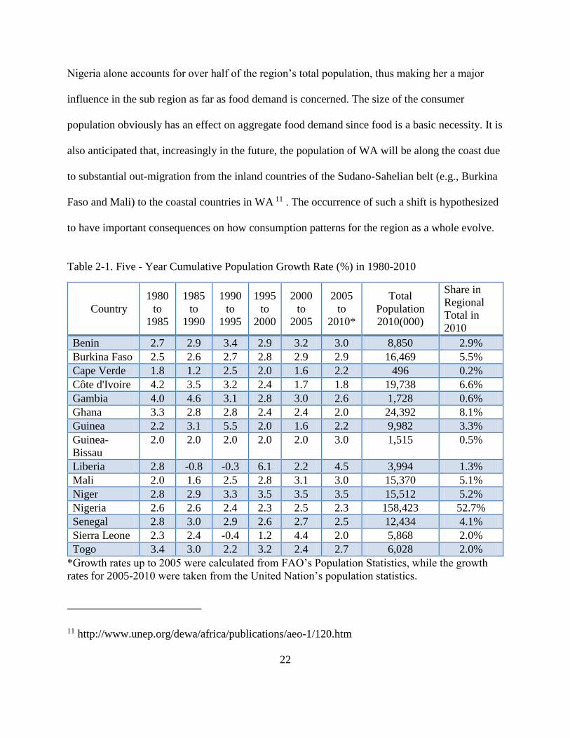
According to the United Nations (2011)10, the 15 West African States that constitute ECOWAS
have a population of approximately 250 million people, covering an area of roughly 5 million
km². The average annual population growth rate is reported at 3%, and it is forecasted that the
sub-region’s population will reach 430 million by 2020. Five-year cumulative population growth
rates in the period 1980-2010 reveal positive continual growth for almost all countries in the
region (Table 2-1). The 2010 population figures reveal the overwhelming importance of the
coastal countries (especially Cote d’Ivoire, Ghana and Nigeria) in the region’s total population.
10 http://www.ohchr.org/EN/Countries/AfricaRegion/Pages/WestAfricaSummary1011.aspx
22
Nigeria alone accounts for over half of the region’s total population, thus making her a major
influence in the sub region as far as food demand is concerned. The size of the consumer
population obviously has an effect on aggregate food demand since food is a basic necessity. It is
also anticipated that, increasingly in the future, the population of WA will be along the coast due
to substantial out-migration from the inland countries of the Sudano-Sahelian belt (e.g., Burkina
Faso and Mali) to the coastal countries in WA 11 . The occurrence of such a shift is hypothesized
to have important consequences on how consumption patterns for the region as a whole evolve.
Table 2-1. Five - Year Cumulative Population Growth Rate (%) in 1980-2010
Country
1980
to
1985
1985
to
1990
1990
to
1995
1995
to
2000
2000
to
2005
2005
to
2010*
Total
Population
2010(000)
Share in
Regional
Total in
2010
Benin 2.7 2.9 3.4 2.9 3.2 3.0 8,850 2.9%
Burkina Faso 2.5 2.6 2.7 2.8 2.9 2.9 16,469 5.5%
Cape Verde 1.8 1.2 2.5 2.0 1.6 2.2 496 0.2%
Côte d'Ivoire 4.2 3.5 3.2 2.4 1.7 1.8 19,738 6.6%
Gambia 4.0 4.6 3.1 2.8 3.0 2.6 1,728 0.6%
Ghana 3.3 2.8 2.8 2.4 2.4 2.0 24,392 8.1%
Guinea 2.2 3.1 5.5 2.0 1.6 2.2 9,982 3.3%
Guinea-
Bissau
2.0 2.0 2.0 2.0 2.0 3.0 1,515 0.5%
Liberia 2.8 -0.8 -0.3 6.1 2.2 4.5 3,994 1.3%
Mali 2.0 1.6 2.5 2.8 3.1 3.0 15,370 5.1%
Niger 2.8 2.9 3.3 3.5 3.5 3.5 15,512 5.2%
Nigeria 2.6 2.6 2.4 2.3 2.5 2.3 158,423 52.7%
Senegal 2.8 3.0 2.9 2.6 2.7 2.5 12,434 4.1%
Sierra Leone 2.3 2.4 -0.4 1.2 4.4 2.0 5,868 2.0%
Togo 3.4 3.0 2.2 3.2 2.4 2.7 6,028 2.0%
*Growth rates up to 2005 were calculated from FAO’s Population Statistics, while the growth
rates for 2005-2010 were taken from the United Nation’s population statistics.
11 http://www.unep.org/dewa/africa/publications/aeo-1/120.htm
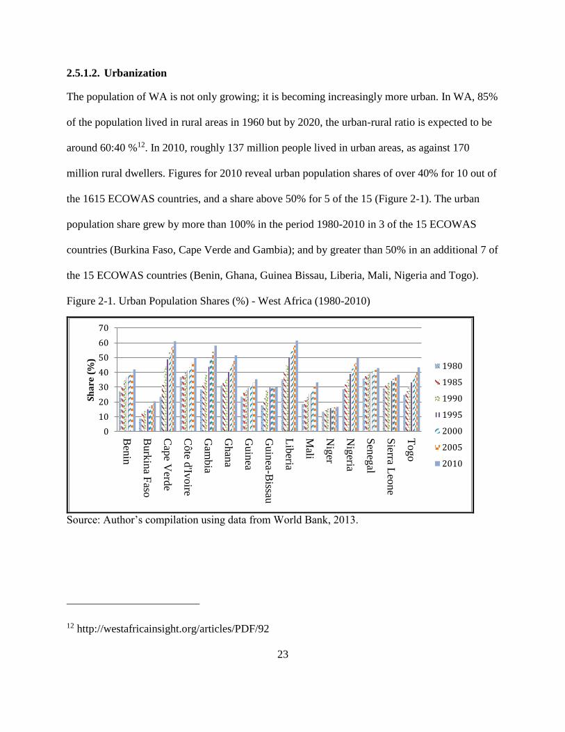
23
2.5.1.2. Urbanization
The population of WA is not only growing; it is becoming increasingly more urban. In WA, 85%
of the population lived in rural areas in 1960 but by 2020, the urban-rural ratio is expected to be
around 60:40 %12. In 2010, roughly 137 million people lived in urban areas, as against 170
million rural dwellers. Figures for 2010 reveal urban population shares of over 40% for 10 out of
the 1615 ECOWAS countries, and a share above 50% for 5 of the 15 (Figure 2-1). The urban
population share grew by more than 100% in the period 1980-2010 in 3 of the 15 ECOWAS
countries (Burkina Faso, Cape Verde and Gambia); and by greater than 50% in an additional 7 of
the 15 ECOWAS countries (Benin, Ghana, Guinea Bissau, Liberia, Mali, Nigeria and Togo).
Figure 2-1. Urban Population Shares (%) - West Africa (1980-2010)
Source: Author’s compilation using data from World Bank, 2013.
12 http://westafricainsight.org/articles/PDF/92
0
10
20
30
40
50
60
70
Ben
in
Burk
ina F
aso
Cap
e Verd
e
Côte d
'Ivoire
Gam
bia
Ghan
a
Guin
ea
Guin
ea-Bissau
Lib
eria
Mali
Nig
er
Nig
eria
Sen
egal
Sierra L
eone
Togo
Sh
are
(%
)
1980
1985
1990
1995
2000
2005
2010
24
The descriptive results presented later in this chapter provide some insight on how food
availability in levels and composition is evolving with the growth in the urban population. The
econometric results presented later in Chapter 3 also serve to provide evidence of any statistical
association between the growth in urban population share and starchy staples availability per
capita.
2.5.1.3. Economic Growth
Changes in consumption patterns have also been associated with changes in a nation’s per capita
gross national product. In economic theory, the relationship between food consumption and
income levels is characterized by Engel’s law–the proportion of income spent on food falls as
income rises. The evolution in real per capita gross domestic product (GDP)–an indicator of
purchasing power, in the region reveals an overall positive trend over the period 1980-2010.
Increases in average annual real per capita GDP growth rates are particularly large in the 2000s
(Table 2-2).
With the exception of a few countries (Cote d’Ivoire, Guinea Bissau, Liberia, Guinea and
Togo), per capita GDP has been growing for most countries since 2000, and the growth rates
have been largest for Cape Verde, Ghana, Nigeria, Burkina Faso, Mali and Sierra Leone. Regmi
and Dyck (2001) observe that urbanization is closely related to economic development and that
both interact to bring about important changes in the composition of consumption—the specific
effects of urbanization on consumption differ depending on the economic conditions.
Urbanization may result in an overall increase in per capita consumption, could result in
improvement in diet quality (such as an increase in animal protein consumption), and could also
increase the demand for processed or easy-to-prepare food (Regmi, 2001).
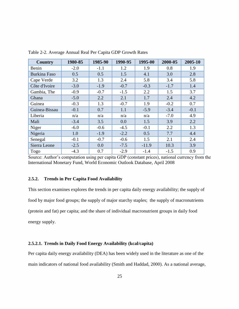
25
Table 2-2. Average Annual Real Per Capita GDP Growth Rates
Country 1980-85 1985-90 1990-95 1995-00 2000-05 2005-10
Benin -2.0 -1.1 1.2 1.9 0.8 1.9
Burkina Faso 0.5 0.5 1.5 4.1 3.0 2.8
Cape Verde 3.2 1.3 2.4 5.8 3.4 5.8
Côte d'Ivoire -3.0 -1.9 -0.7 -0.3 -1.7 1.4
Gambia, The -0.9 -0.7 -1.5 2.2 1.5 3.7
Ghana -5.0 2.2 2.1 1.7 2.4 4.2
Guinea -0.3 1.3 -0.7 1.9 -0.2 0.7
Guinea-Bissau -0.1 0.7 1.1 -5.9 -3.4 -0.1
Liberia n/a n/a n/a n/a -7.0 4.9
Mali -3.4 3.5 0.0 1.5 3.9 2.2
Niger -6.0 -0.6 -4.5 -0.1 2.2 1.3
Nigeria 1.0 -1.9 -2.2 0.5 7.7 4.4
Senegal -0.1 -0.7 -0.6 1.5 2.1 2.4
Sierra Leone -2.5 0.0 -7.5 -11.9 10.3 3.9
Togo -4.3 0.7 -2.9 -1.4 -1.5 0.9
Source: Author’s computation using per capita GDP (constant prices), national currency from the
International Monetary Fund, World Economic Outlook Database, April 2008
2.5.2. Trends in Per Capita Food Availability
This section examines explores the trends in per capita daily energy availability; the supply of
food by major food groups; the supply of major starchy staples; the supply of macronutrients
(protein and fat) per capita; and the share of individual macronutrient groups in daily food
energy supply.
2.5.2.1. Trends in Daily Food Energy Availability (kcal/capita)
Per capita daily energy availability (DEA) has been widely used in the literature as one of the
main indicators of national food availability (Smith and Haddad, 2000). As a national average,
26
DEA is an imperfect indicator of the state of individual food security. However, empirical
evidence, such as that provided by Smith and Haddad (2000), suggest that there is a strong
correlation between this per capita DEA and more individual-based indicators of food security
(e.g., anthropometric indicators of children’s nutritional status). In particular, Smith and Haddad
(2000) show that national caloric availability was responsible for more than a quarter of
reductions in child malnutrition in developing countries over the period 1970-95. The positive
growth in per capita incomes in the region over time (Table 2-2) is expected to have had a
positive influence on DEA per capita.
The empirical data reveal an overall positive trend in reported total per capita DEA,
particularly in the last two decades (Figures 2-2, 2-3, and 2-4). Burkina Faso, Mali, Ghana, and
Nigeria experienced the largest growth (in relative terms) in reported per capita DEA (50% or
more) between 1980-85 and 2004-09. Cote d’Ivoire and Liberia in the same period experienced a
decline in per capita DEA.
The analysis of the trend in per capita DEA reveals that although the overall pattern for
all countries in the region shows a shift towards greater calorie availability, the magnitude of
growth has greatly varied and has been influenced by factors specific to each country. The
analysis highlights the possible effect of growth in income on per capita DEA. In the Non-
Coastal Sahel (Figure 2-2) for instance, Mali and Burkina Faso, with modest economic growth,
have also shown modest increases (in absolute terms) in per capita DEA over time. Reported per
capita DEA for Mali had the biggest growth in the early and mid-1980s. Compared to the period
1983-85 (characterized by drought and economic crisis in Mali), the period 1986-1988 was
characterized by good harvests and improved economic performance (growth in real per capita
incomes of about 3.5%), which corresponded with growth in per capita DEA of about 18%. Mali
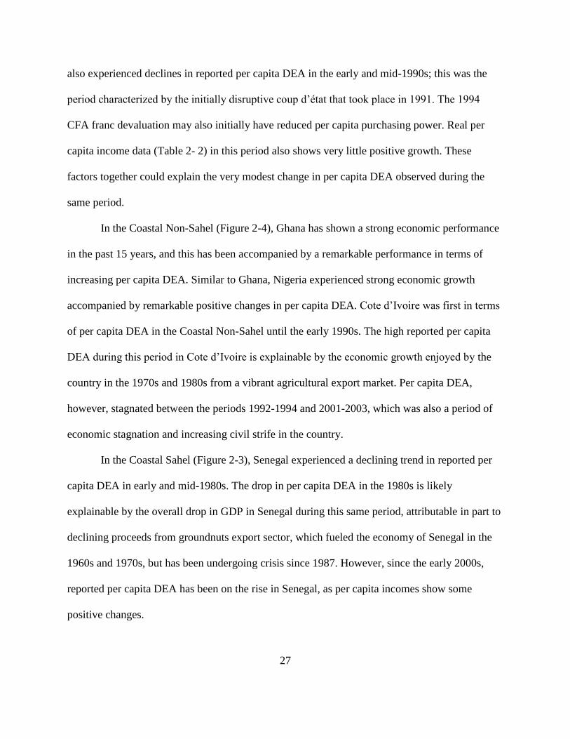
27
also experienced declines in reported per capita DEA in the early and mid-1990s; this was the
period characterized by the initially disruptive coup d’état that took place in 1991. The 1994
CFA franc devaluation may also initially have reduced per capita purchasing power. Real per
capita income data (Table 2- 2) in this period also shows very little positive growth. These
factors together could explain the very modest change in per capita DEA observed during the
same period.
In the Coastal Non-Sahel (Figure 2-4), Ghana has shown a strong economic performance
in the past 15 years, and this has been accompanied by a remarkable performance in terms of
increasing per capita DEA. Similar to Ghana, Nigeria experienced strong economic growth
accompanied by remarkable positive changes in per capita DEA. Cote d’Ivoire was first in terms
of per capita DEA in the Coastal Non-Sahel until the early 1990s. The high reported per capita
DEA during this period in Cote d’Ivoire is explainable by the economic growth enjoyed by the
country in the 1970s and 1980s from a vibrant agricultural export market. Per capita DEA,
however, stagnated between the periods 1992-1994 and 2001-2003, which was also a period of
economic stagnation and increasing civil strife in the country.
In the Coastal Sahel (Figure 2-3), Senegal experienced a declining trend in reported per
capita DEA in early and mid-1980s. The drop in per capita DEA in the 1980s is likely
explainable by the overall drop in GDP in Senegal during this same period, attributable in part to
declining proceeds from groundnuts export sector, which fueled the economy of Senegal in the
1960s and 1970s, but has been undergoing crisis since 1987. However, since the early 2000s,
reported per capita DEA has been on the rise in Senegal, as per capita incomes show some
positive changes.
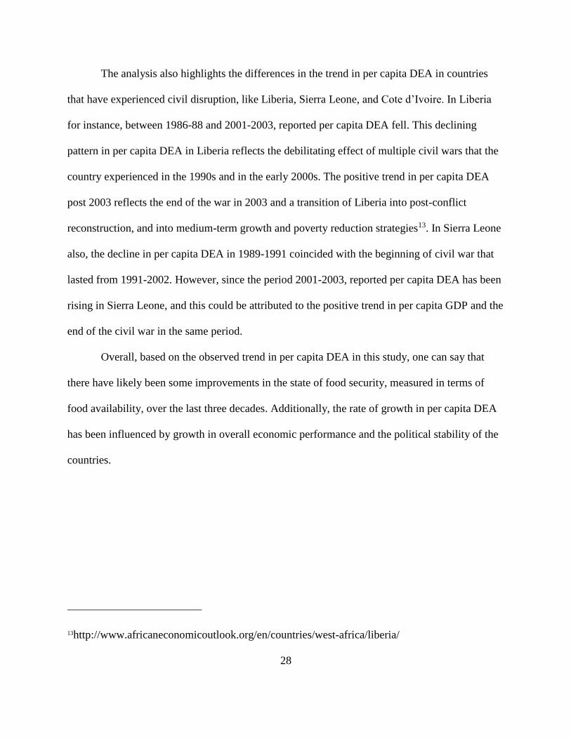
28
The analysis also highlights the differences in the trend in per capita DEA in countries
that have experienced civil disruption, like Liberia, Sierra Leone, and Cote d’Ivoire. In Liberia
for instance, between 1986-88 and 2001-2003, reported per capita DEA fell. This declining
pattern in per capita DEA in Liberia reflects the debilitating effect of multiple civil wars that the
country experienced in the 1990s and in the early 2000s. The positive trend in per capita DEA
post 2003 reflects the end of the war in 2003 and a transition of Liberia into post-conflict
reconstruction, and into medium-term growth and poverty reduction strategies13. In Sierra Leone
also, the decline in per capita DEA in 1989-1991 coincided with the beginning of civil war that
lasted from 1991-2002. However, since the period 2001-2003, reported per capita DEA has been
rising in Sierra Leone, and this could be attributed to the positive trend in per capita GDP and the
end of the civil war in the same period.
Overall, based on the observed trend in per capita DEA in this study, one can say that
there have likely been some improvements in the state of food security, measured in terms of
food availability, over the last three decades. Additionally, the rate of growth in per capita DEA
has been influenced by growth in overall economic performance and the political stability of the
countries.
13http://www.africaneconomicoutlook.org/en/countries/west-africa/liberia/
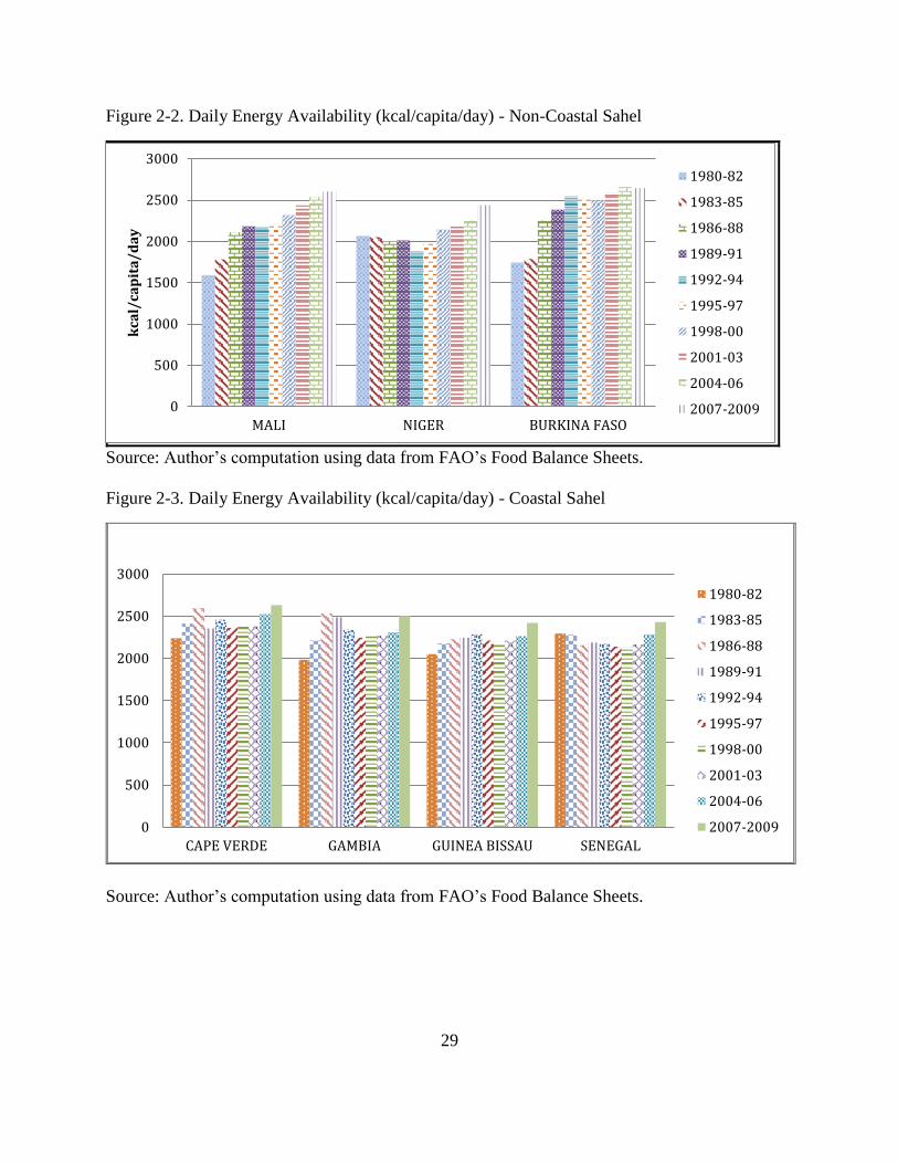
29
Figure 2-2. Daily Energy Availability (kcal/capita/day) - Non-Coastal Sahel
Source: Author’s computation using data from FAO’s Food Balance Sheets.
Figure 2-3. Daily Energy Availability (kcal/capita/day) - Coastal Sahel
Source: Author’s computation using data from FAO’s Food Balance Sheets.
0
500
1000
1500
2000
2500
3000
MALI NIGER BURKINA FASO
kca
l/ca
pit
a/
da
y
1980-82
1983-85
1986-88
1989-91
1992-94
1995-97
1998-00
2001-03
2004-06
2007-2009
0
500
1000
1500
2000
2500
3000
CAPE VERDE GAMBIA GUINEA BISSAU SENEGAL
1980-82
1983-85
1986-88
1989-91
1992-94
1995-97
1998-00
2001-03
2004-06
2007-2009
30
Figure 2-4. Daily Energy Availability (kcal/capita/day) - Coastal Non-Sahel
Source: Author’s computation using data from FAO’s Food Balance Sheets.
2.5.2.2 Trends in the Composition of Per Capita Food Availability by Major Food Group
This sub-section examines aggregate shifts in per capita food supply by major food group.
Specifically, it examines whether there has been a diversification in the composition of food
supply, whereby new food groups (e.g., starchy roots and tubers (R&T) in the non-Coastal Sahel)
are emerging as important contributors to the reported per capita DEA. There are some
differences in major food groups across sub-regions. However, the most common food groups in
this analysis are cereals (excluding beer), starchy R&T, fruits (excluding wine), vegetables,
vegetable oils, meats and offal, alcoholic beverages, oilcrops, sugars and sweeteners, pulses,
milk (excluding butter), and fish and seafood. The trend in a major food group, say “starchy
R&T,” may not reflect what changes are taking place with respect to the supply of a specific
0
500
1000
1500
2000
2500
3000
3500
kca
l/ca
pit
a/d
ay
1980-82
1983-85
1986-88
1989-91
1992-94
1995-97
1998-00
2001-03
2004-06
2007-2009
31
starchy R&T type (e.g., cassava or potatoes). The next sub-section examines trends in specific
commodities within major staple food categories.
2.5.2.2.1. Non-Coastal Sahel
Cereals are the dominant food group in the Non-Coastal Sahel. Per capita cereals availability (in
terms of kg/person) increased by 44% for Mali (Table A2-2 in Appendix), 55% for Burkina Faso
(Table A2-1 in Appendix), and by only 3% in Niger (Table A2-3 in Appendix) during the study
period. Mali alone experienced an increase in per capita availability of starchy R&T in this sub-
region. Per capita starchy R&T supply declined in Burkina Faso (56%) and Niger (57%), albeit
from small initial levels. Niger experienced the largest positive change in per capita availability
of vegetables—from an average of 16 kg/capita/year in the period 1983-1985 to 51
kg/capita/year in 2007-2009 – an increase of 170% in the study period. In Mali, vegetable supply
increased by 4%, while Burkina Faso experienced a decline of 27 %, in the study period.
Reported availability of fruits rose in Niger (93%) and Mali (71%), while Burkina Faso
experienced a decline of 38%. Reported per capita supply of meats and offal increased by 45%
for Mali, 85% for Burkina Faso and 12% for Niger in the period from 1980-85 through to 2004-
2009.
A possible explanation for the higher supplies and higher rate of growth in the per capita
supply of meats and offal in Mali and Burkina compared to Niger is the higher per capita
incomes in Mali and Burkina Faso and economic stagnation in Niger. In contrast, in Niger,
consumers appear to have relied more on pulses (particularly cowpeas) as a major, and lower-
cost, source of protein in the diet. Per capita supply of pulses increased in Niger by 44% in the
period 1980-85 to 2004-09. In this sub-region, per capita supply of alcoholic beverages is highest
32
for Burkina Faso–and has generally remained above an average of 50 kg/capita/year in that
country.
2.5.2.2.2. Coastal Non-Sahel
Starchy R&T compete with cereals as major calorie sources in this sub-region. Cereals supply
per capita has been on the rise for all countries in this sub-region. For all Coastal Non-Sahelian
countries except Sierra Leone, starchy R&T supply has been greater than 100 kg/capita/year
since the 1980s. Ghana (Table A2-6 in Appendix) and Nigeria (Table A2-9 in Appendix )
experienced the most noticeable growth in per capita supply of starchy R&T (72% and 117%
respectively), and in both countries starchy R&T supply was about double that of cereals. The
sharp increase in the supply of starchy R&T per capita in Nigeria from an average of 111 kg/year
in 1986-1988 to 231 kg/year in 1992-1994 reflected the “cassava revolution” in Nigeria (Nweke
et al., 2002).
Ghana experienced an increase in per capita supply of almost all major food groups in the
study period. Fruit supply per capita increased dramatically from an average of 86 kg/year in the
period 1980-85 to 147 kg/year in 2004-09, an increase of 72%; meats and offal supply increased
by about 22% (absolute supply stayed below 15 kg/capita/year); milk supply per capita rose by
about 129%; vegetable oil supply increased by 55%; fish and seafood by 36%; and the supply of
alcoholic beverages rose by about 26%. Nigeria, on the other hand, experienced a decline in per
capita supply of meats and offal of 12%. However, the per capita supply of pulses (a source of
high-quality protein) increased dramatically in Nigeria by 138%. Vegetable oil supply per capita
also increased by 50% in Nigeria.
33
2.5.2.2.3. Coastal Sahel
In the Coastal Sahel, cereals are still a major food group. Based on per capita availability, other
major food groups in this region are fruits and vegetables, meats and offal, milk, sugars and
sweeteners, fish and seafood. Although cereals are a major component of food availability in this
sub-region, over time, per capita cereals supply did not change very much. Compared to the
Coastal non-Sahel sub-region, the per capita supply of starchy R&T is much lower in this sub-
region. In Cape Verde, the starchy R&T supply per capita increased by 69% in the study period
(Table A2-12 in Appendix). Senegal also experienced dramatic changes (especially in the 2000s)
in the starchy R&T supply per capita—from an average of 8 kg/year in 1980-1982 to 29 kg/year
in 2007-2009, an increase of 247% (Table A2-15 in Appendix). Cape Verde, which experienced
rapid economic growth and has the highest per-capita income in the sub-region, experienced an
increase in the supply of almost all major food groups in the study period: per capita supply of
fruit by 106%; that of vegetables by 777%; that of meats and offal by 332%; that of milk supply
by 69%; that of eggs by 300%; that of sugars and sweeteners by 69% and that of alcoholic
beverages by 200%. In contrast, the per capita availability of pulses decreased by 27% and that
of fish and seafood declined by 59%.
Senegal has also shown a positive trend in the supply of all major food groups (Table A2-
15 in Appendix). In the period of study in Senegal, vegetable supply per capita increased from an
average of 17 kg/year in 1980-1982 to 64 kg/year in 2007-2009–an overall increase of 269%;
fruit supply remained at less than 20 kg/capita/year, and increased by 29%; the supply of meats
and offal per capita increased by 23% per capita; and fish and seafood supply (highest per capita
for Senegal in this sub-region) increased by 16%. With the exception of cereals, starchy R&T,
alcoholic beverages and fruits, the supply of all other major food groups remained below 20
34
kg/capita/year in Guinea Bissau (Table A2-14 in Appendix). Food supply per capita in the
Gambia also did not show any striking changes over time (Table A2-13 in Appendix).
Overall, in the Coastal Sahel region, the most noticeable change in the supply of food by
major food group has been in the case of starchy R&T in Cape Verde and Senegal. The specific
composition of these changes in major starchy staples food groups (cereals and roots and tubers)
are investigated in the next sub section.
Overall, the analysis of trends in per capita food availability in the ECOWAS states
shows the following trends in food supply by major food groups. In the Sahel region, we observe
an increase in the supply of starchy R&T (e.g., in Mali, Senegal and Cape Verde). In most
countries across all sub regions, we observe an increase in the per capita supply of fruits and
vegetables, and also of meats and offal. However, while cereals have been for a long time basic
staples in the Sahel and as such most fully reported in official production statistics, agricultural
production statistics in underdeveloped low-income countries have been criticized for being
deficient in the reporting of figures for crops like cassava, fruits and vegetables as well as
livestock (Farnsworth, 1961). Hence, this raises a question of the extent to which the apparent
diversification (more starchy staples, more fruits and vegetables) of the diet (in terms of major
commodities) over time shown by the FBS reflects real diversification versus just an
improvement in the ability of national agricultural statistics to capture non-cereal production
(e.g., roots, tubers and horticultural products).
2.5.2.3. Trends in the Availability of Major Starchy Staple Types (kg/capita/year)
This sub-section examines the trends in the availability of specific starchy staples for a better
understanding of the dynamics of food supply in the region. Disaggregating major starchy staple
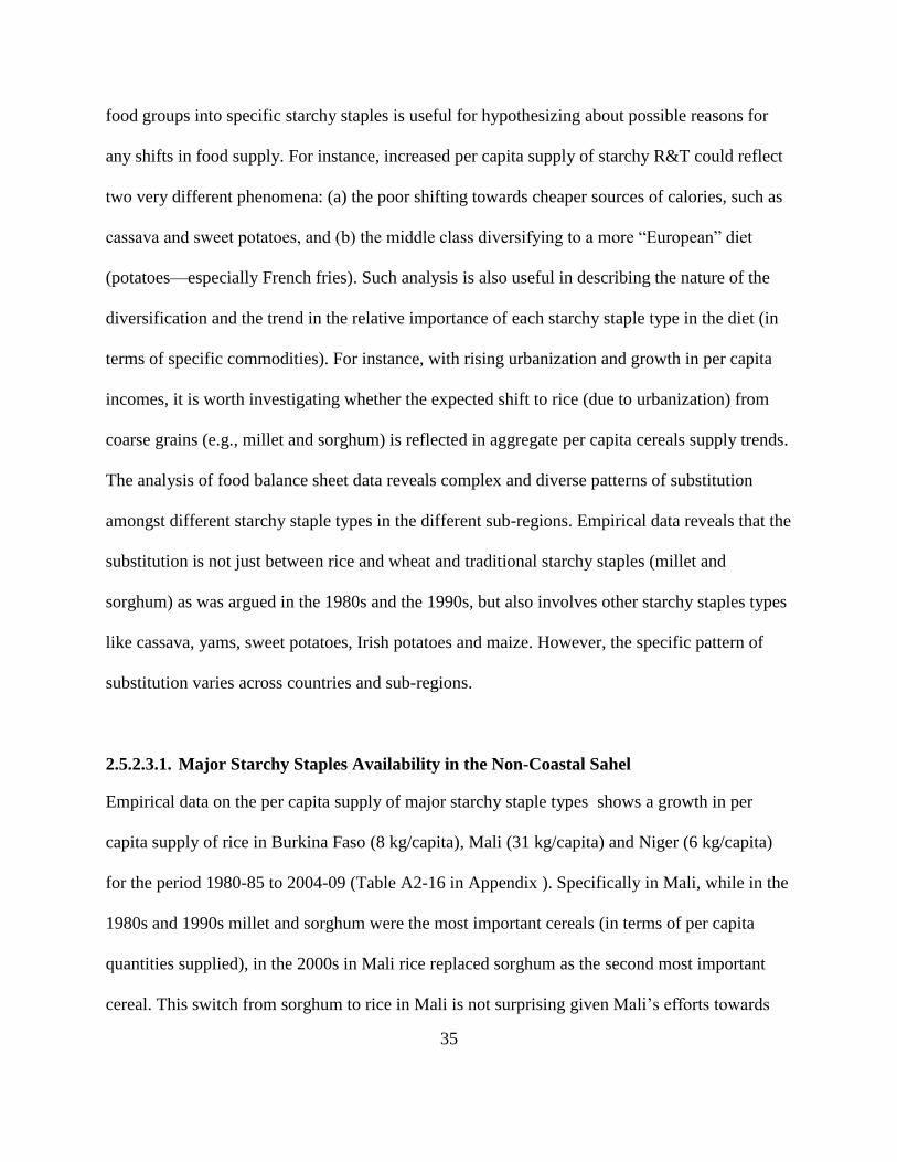
35
food groups into specific starchy staples is useful for hypothesizing about possible reasons for
any shifts in food supply. For instance, increased per capita supply of starchy R&T could reflect
two very different phenomena: (a) the poor shifting towards cheaper sources of calories, such as
cassava and sweet potatoes, and (b) the middle class diversifying to a more “European” diet
(potatoes—especially French fries). Such analysis is also useful in describing the nature of the
diversification and the trend in the relative importance of each starchy staple type in the diet (in
terms of specific commodities). For instance, with rising urbanization and growth in per capita
incomes, it is worth investigating whether the expected shift to rice (due to urbanization) from
coarse grains (e.g., millet and sorghum) is reflected in aggregate per capita cereals supply trends.
The analysis of food balance sheet data reveals complex and diverse patterns of substitution
amongst different starchy staple types in the different sub-regions. Empirical data reveals that the
substitution is not just between rice and wheat and traditional starchy staples (millet and
sorghum) as was argued in the 1980s and the 1990s, but also involves other starchy staples types
like cassava, yams, sweet potatoes, Irish potatoes and maize. However, the specific pattern of
substitution varies across countries and sub-regions.
2.5.2.3.1. Major Starchy Staples Availability in the Non-Coastal Sahel
Empirical data on the per capita supply of major starchy staple types shows a growth in per
capita supply of rice in Burkina Faso (8 kg/capita), Mali (31 kg/capita) and Niger (6 kg/capita)
for the period 1980-85 to 2004-09 (Table A2-16 in Appendix ). Specifically in Mali, while in the
1980s and 1990s millet and sorghum were the most important cereals (in terms of per capita
quantities supplied), in the 2000s in Mali rice replaced sorghum as the second most important
cereal. This switch from sorghum to rice in Mali is not surprising given Mali’s efforts towards
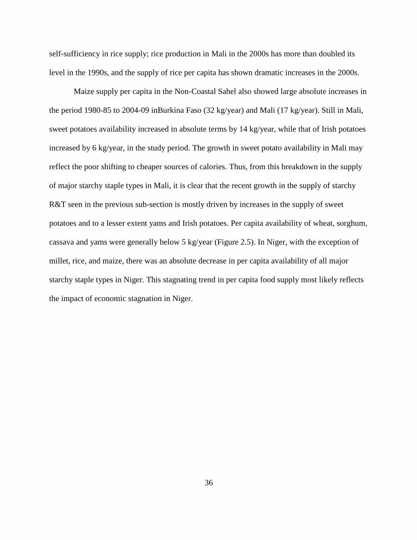
36
self-sufficiency in rice supply; rice production in Mali in the 2000s has more than doubled its
level in the 1990s, and the supply of rice per capita has shown dramatic increases in the 2000s.
Maize supply per capita in the Non-Coastal Sahel also showed large absolute increases in
the period 1980-85 to 2004-09 inBurkina Faso (32 kg/year) and Mali (17 kg/year). Still in Mali,
sweet potatoes availability increased in absolute terms by 14 kg/year, while that of Irish potatoes
increased by 6 kg/year, in the study period. The growth in sweet potato availability in Mali may
reflect the poor shifting to cheaper sources of calories. Thus, from this breakdown in the supply
of major starchy staple types in Mali, it is clear that the recent growth in the supply of starchy
R&T seen in the previous sub-section is mostly driven by increases in the supply of sweet
potatoes and to a lesser extent yams and Irish potatoes. Per capita availability of wheat, sorghum,
cassava and yams were generally below 5 kg/year (Figure 2.5). In Niger, with the exception of
millet, rice, and maize, there was an absolute decrease in per capita availability of all major
starchy staple types in Niger. This stagnating trend in per capita food supply most likely reflects
the impact of economic stagnation in Niger.
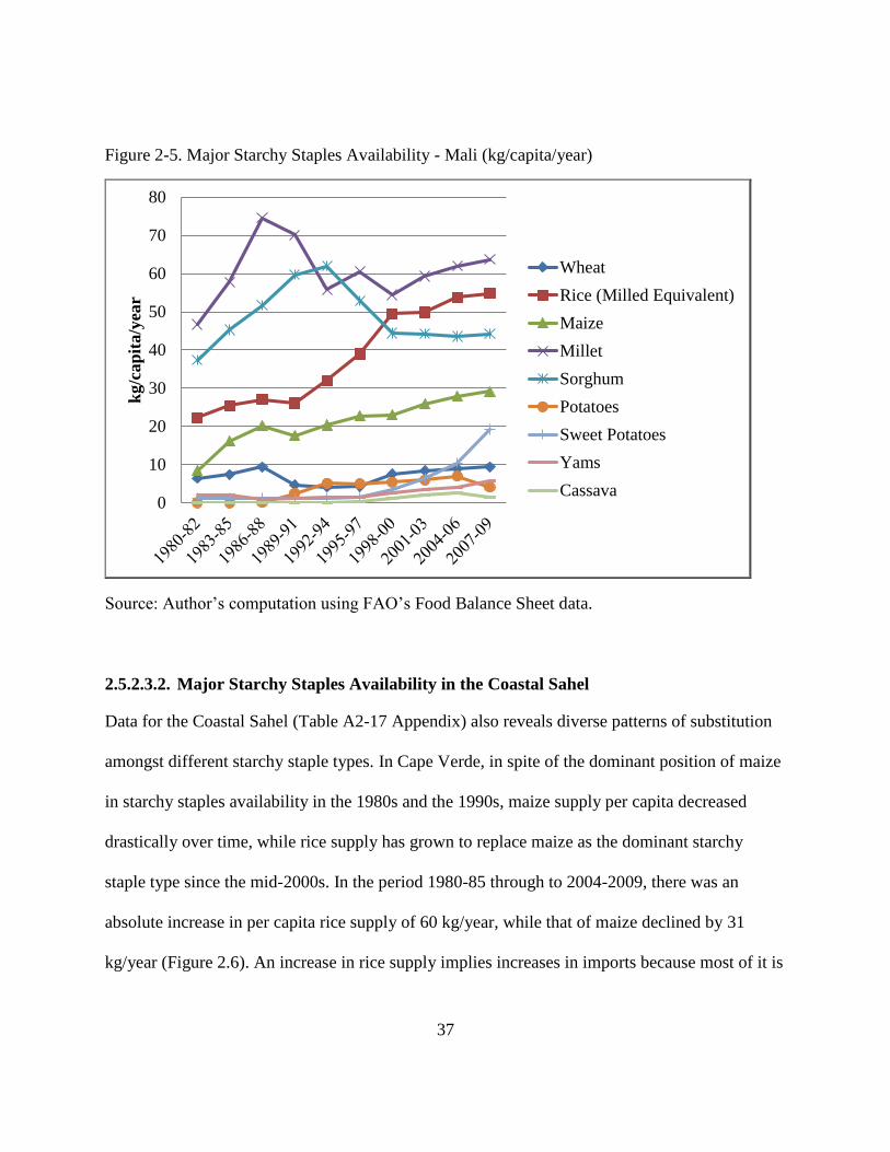
37
Figure 2-5. Major Starchy Staples Availability - Mali (kg/capita/year)
Source: Author’s computation using FAO’s Food Balance Sheet data.
2.5.2.3.2. Major Starchy Staples Availability in the Coastal Sahel
Data for the Coastal Sahel (Table A2-17 Appendix) also reveals diverse patterns of substitution
amongst different starchy staple types. In Cape Verde, in spite of the dominant position of maize
in starchy staples availability in the 1980s and the 1990s, maize supply per capita decreased
drastically over time, while rice supply has grown to replace maize as the dominant starchy
staple type since the mid-2000s. In the period 1980-85 through to 2004-2009, there was an
absolute increase in per capita rice supply of 60 kg/year, while that of maize declined by 31
kg/year (Figure 2.6). An increase in rice supply implies increases in imports because most of it is
0
10
20
30
40
50
60
70
80
kg/c
ap
ita/y
ear
Wheat
Rice (Milled Equivalent)
Maize
Millet
Sorghum
Potatoes
Sweet Potatoes
Yams
Cassava
38
imported14 . Alongside the big increase in per capita rice availability in Cape Verde has been a
rapid growth in the supply of Irish potatoes, whereby the per capita supply of Irish potatoes rose
from an average of 11 kg/year in the period 1980-1985 to an average of 29 kg/year in 2004-2009.
Figure 2-6. Major Starchy Staples Availability - Cape Verde (kg/capita/year)
Source: Author’s computation using FAO’s Food Balance Sheet data.
In Senegal, rice was the dominant starchy staple type (greater than 55 kg/capita/year)
throughout the study period. However, per capita maize availability increased (by 13kg/year)
more than that of rice (5 kg/year) over the 30-year period (Figure 2-7). Senegal also experienced
a very sharp decline in millet and sorghum availability per capita. This reflects a major shift in
the composition of the average diet, linked possibly to urbanization. Furthermore, wheat
availability per capita also increased in Senegal by 12 kg/year during the study period. Increases
14 FAO’s FBS reveal rice production data for Cape Verde of less than 1000 tons throughout the
period 1980-2009, while rice imports increased from an average of 10,000 tons in the period
1980-84 to 46,000 tons in 2005-09.
0
10
20
30
40
50
60
70
80
90
100
kg/c
ap
ita/y
ear
Wheat
Rice (Milled
Equivalent)
Maize
Cassava
Potatoes
Sweet Potatoes
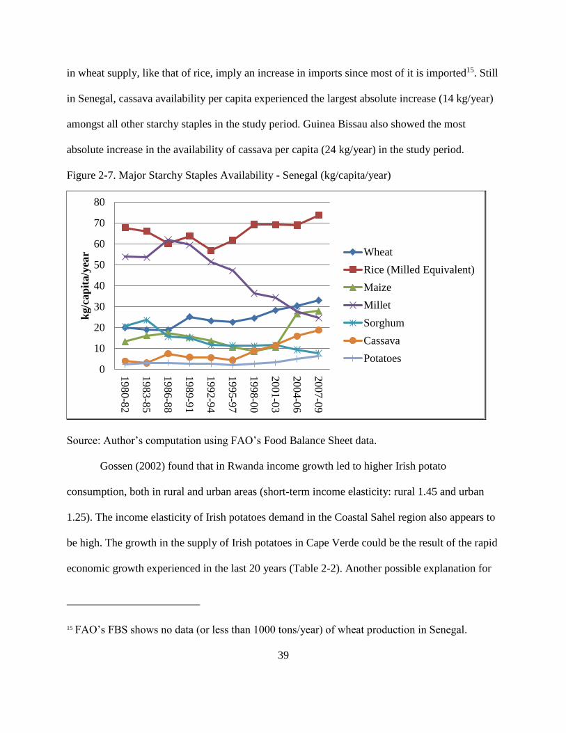
39
in wheat supply, like that of rice, imply an increase in imports since most of it is imported15. Still
in Senegal, cassava availability per capita experienced the largest absolute increase (14 kg/year)
amongst all other starchy staples in the study period. Guinea Bissau also showed the most
absolute increase in the availability of cassava per capita (24 kg/year) in the study period.
Figure 2-7. Major Starchy Staples Availability - Senegal (kg/capita/year)
Source: Author’s computation using FAO’s Food Balance Sheet data.
Gossen (2002) found that in Rwanda income growth led to higher Irish potato
consumption, both in rural and urban areas (short-term income elasticity: rural 1.45 and urban
1.25). The income elasticity of Irish potatoes demand in the Coastal Sahel region also appears to
be high. The growth in the supply of Irish potatoes in Cape Verde could be the result of the rapid
economic growth experienced in the last 20 years (Table 2-2). Another possible explanation for
15 FAO’s FBS shows no data (or less than 1000 tons/year) of wheat production in Senegal.
0
10
20
30
40
50
60
70
80
1980-8
2
1983-8
5
1986-8
8
1989-9
1
1992-9
4
1995-9
7
1998-0
0
2001-0
3
2004-0
6
2007-0
9
kg/c
ap
ita/y
ear Wheat
Rice (Milled Equivalent)
Maize
Millet
Sorghum
Cassava
Potatoes
40
the growth in the supply of Irish potatoes in Cape Verde is changes in lifestyle–i.e., growth in the
consumption of more potato chips (French fries) as people adopt a more Western diet. While the
growth in the supply of Irish potatoes could be the result of the westernization of diets and
economic growth, the rapid growth in the supply of cassava (Senegal and Guinea Bissau), and to
a lesser extent sweet potatoes (Senegal) may represent a shift of the poor to cheaper sources of
calories.
Also from empirical data, millet appears to be replacing rice in terms of per capita
availability in the Gambia. The absolute change in per capita availability was plus 27 kg/year
for millet and minus 34 kg/year for rice in the period 1980-85 through to 2004-09. However, it is
worth pointing out that prior to the CFA franc devaluation, The Gambia had a large re-
exportation trade of imported rice to Senegal. The drastic decline in per capita rice availability
may just reflect the decline in those largely unrecorded previous re-exportations.
2.5.2.3.3. Major Starchy Staples Availability in the Coastal Non-Sahel
Empirical data on the per capita supply of major starchy staple types in the Coastal non-Sahel
region reveals remarkable increases in the supply of starchy roots and tubers and to a lesser
extent cereals (Table A2-18 Appendix). Ghana for example, experienced an absolute increase in
per capita availability of cassava of 86 kg/year, while that of yams increased by 67 kg/year.
Nigeria also experienced the largest absolute increases in per capita availability with cassava (36
kg/year) and with yams (57 kg/year). Per capita availability of sweet potatoes also increased in
Nigeria by 14 kg/year and that of Irish potatoes by 4 kg/year in the study period. In Benin, per
capita availability increased the most for yams (56 kg/year) and cassava (25 kg/year). In Guinea
41
and Sierra Leone also, cassava availability per capita increased by 13 kg/year and 36 kg/year
respectively in the period 1980-85 through to 2004-09.
The increases in the annual per capita supply of specific cereals for Ghana were as
follows: rice, 19 kg; wheat, 8 kg; and maize, 6 kg. In Nigeria, the increases in annual per capita
availability over the study period were maize, 17 kg; wheat, 4 kg; rice, 7 kg; millet,16 10 kg and
sorghum, 6 kg. Benin also experienced an increase in per capita availability of rice (22 kg/year)
in the study period. However, given the importance of unrecorded trade between Benin and
Nigeria, it is possible that some of the increase in recorded per capita rice availability in Benin
actually represented rice transshipped into Nigeria. Maize has over the years maintained its
position as the dominant cereal type in Benin. However, per capita maize consumption increased
only by 3 kg/year in the period 1980-85 through to 2004-09. Rice availability per capita also
increased by 27 kg/year in Guinea in the period 1980-85 through to 2004-09.
Contrary to the increase in rice supply in the other countries in this sub-region, rice
supply per capita decreased by 7 kg/year in Sierra Leone and by 48 kg/year in Liberia during the
study period. For Sierra Leone, the growth in per capita availability of cassava and the decline in
rice availability per capita reflect some degree of substitution of cassava for rice, since both
crops have been over time major starchy staples in Sierra Leone. For Liberia, following a period
of low and relatively stable supply of wheat in the 1980s, per capita wheat supply jumped from
an average of 9 kg/capita/year in the period 1992-1994 to 52 kg/capita/year in the period 1995-
16 Nigeria has the largest apparent per capita supply of millet in the Coastal Non-Sahel. This is not
surprising because Nigeria is the only one of these countries that also has a large Sudano-Sahelian
zone, which is the major area where millet is produced.
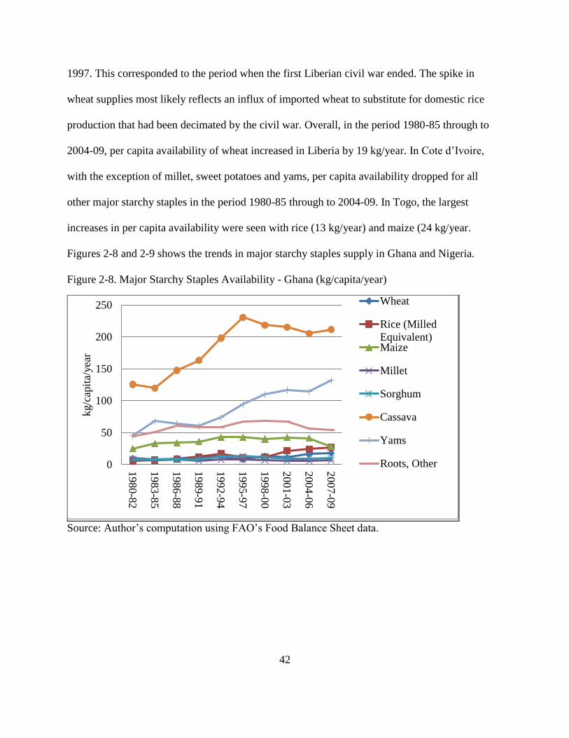
42
1997. This corresponded to the period when the first Liberian civil war ended. The spike in
wheat supplies most likely reflects an influx of imported wheat to substitute for domestic rice
production that had been decimated by the civil war. Overall, in the period 1980-85 through to
2004-09, per capita availability of wheat increased in Liberia by 19 kg/year. In Cote d’Ivoire,
with the exception of millet, sweet potatoes and yams, per capita availability dropped for all
other major starchy staples in the period 1980-85 through to 2004-09. In Togo, the largest
increases in per capita availability were seen with rice (13 kg/year) and maize (24 kg/year.
Figures 2-8 and 2-9 shows the trends in major starchy staples supply in Ghana and Nigeria.
Figure 2-8. Major Starchy Staples Availability - Ghana (kg/capita/year)
Source: Author’s computation using FAO’s Food Balance Sheet data.
0
50
100
150
200
250
1980-8
2
1983-8
5
1986-8
8
1989-9
1
1992-9
4
1995-9
7
1998-0
0
2001-0
3
2004-0
6
2007-0
9
kg/c
apit
a/yea
r
Wheat
Rice (Milled
Equivalent)Maize
Millet
Sorghum
Cassava
Yams
Roots, Other
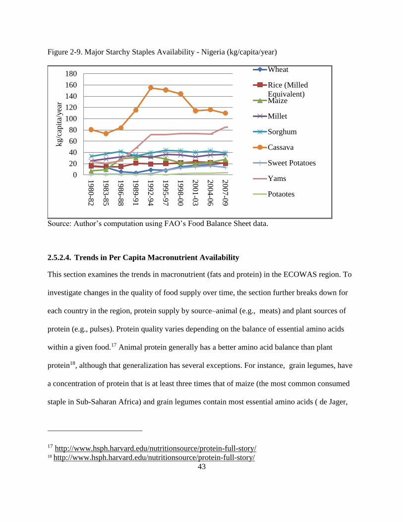
43
Figure 2-9. Major Starchy Staples Availability - Nigeria (kg/capita/year)
Source: Author’s computation using FAO’s Food Balance Sheet data.
2.5.2.4. Trends in Per Capita Macronutrient Availability
This section examines the trends in macronutrient (fats and protein) in the ECOWAS region. To
investigate changes in the quality of food supply over time, the section further breaks down for
each country in the region, protein supply by source–animal (e.g., meats) and plant sources of
protein (e.g., pulses). Protein quality varies depending on the balance of essential amino acids
within a given food.17 Animal protein generally has a better amino acid balance than plant
protein18, although that generalization has several exceptions. For instance, grain legumes, have
a concentration of protein that is at least three times that of maize (the most common consumed
staple in Sub-Saharan Africa) and grain legumes contain most essential amino acids ( de Jager,
17 http://www.hsph.harvard.edu/nutritionsource/protein-full-story/ 18 http://www.hsph.harvard.edu/nutritionsource/protein-full-story/
0
20
40
60
80
100
120
140
160
180
1980-8
2
1983-8
5
1986-8
8
1989-9
1
1992-9
4
1995-9
7
1998-0
0
2001-0
3
2004-0
6
2007-0
9
kg/c
apit
a/yea
r
Wheat
Rice (Milled
Equivalent)Maize
Millet
Sorghum
Cassava
Sweet Potatoes
Yams
Potaotes
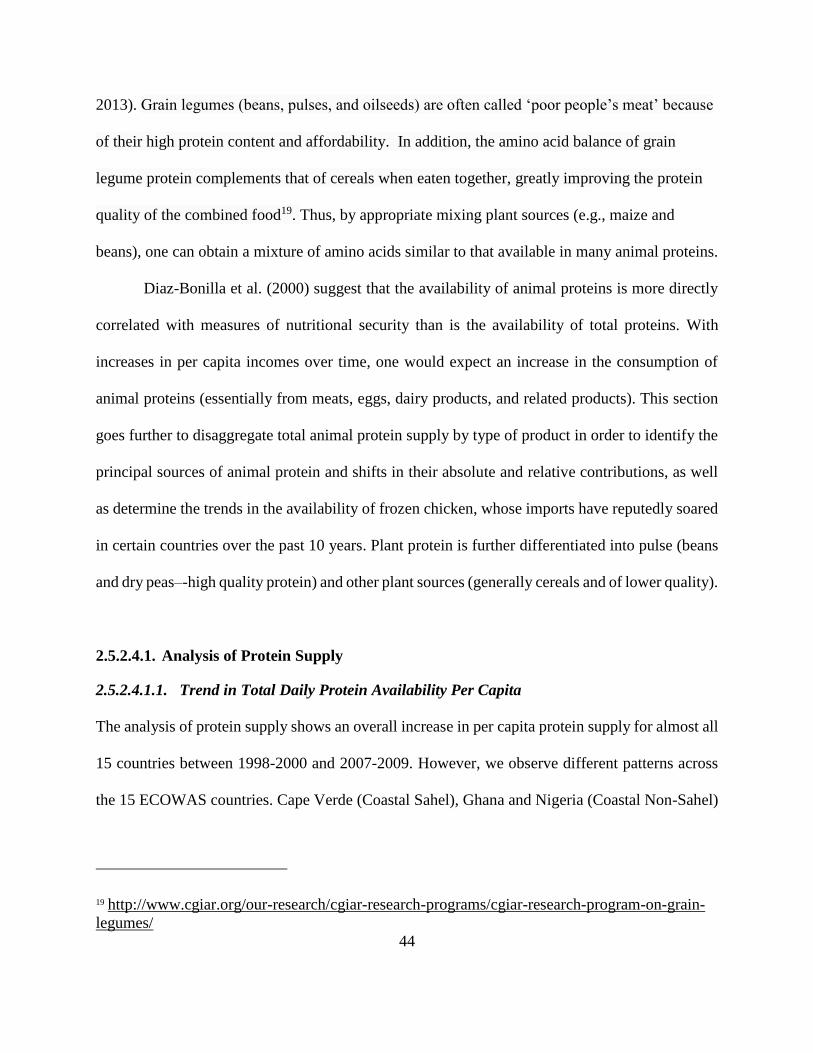
44
2013). Grain legumes (beans, pulses, and oilseeds) are often called ‘poor people’s meat’ because
of their high protein content and affordability. In addition, the amino acid balance of grain
legume protein complements that of cereals when eaten together, greatly improving the protein
quality of the combined food19. Thus, by appropriate mixing plant sources (e.g., maize and
beans), one can obtain a mixture of amino acids similar to that available in many animal proteins.
Diaz-Bonilla et al. (2000) suggest that the availability of animal proteins is more directly
correlated with measures of nutritional security than is the availability of total proteins. With
increases in per capita incomes over time, one would expect an increase in the consumption of
animal proteins (essentially from meats, eggs, dairy products, and related products). This section
goes further to disaggregate total animal protein supply by type of product in order to identify the
principal sources of animal protein and shifts in their absolute and relative contributions, as well
as determine the trends in the availability of frozen chicken, whose imports have reputedly soared
in certain countries over the past 10 years. Plant protein is further differentiated into pulse (beans
and dry peas–-high quality protein) and other plant sources (generally cereals and of lower quality).
2.5.2.4.1. Analysis of Protein Supply
2.5.2.4.1.1. Trend in Total Daily Protein Availability Per Capita
The analysis of protein supply shows an overall increase in per capita protein supply for almost all
15 countries between 1998-2000 and 2007-2009. However, we observe different patterns across
the 15 ECOWAS countries. Cape Verde (Coastal Sahel), Ghana and Nigeria (Coastal Non-Sahel)
19 http://www.cgiar.org/our-research/cgiar-research-programs/cgiar-research-program-on-grain-
legumes/
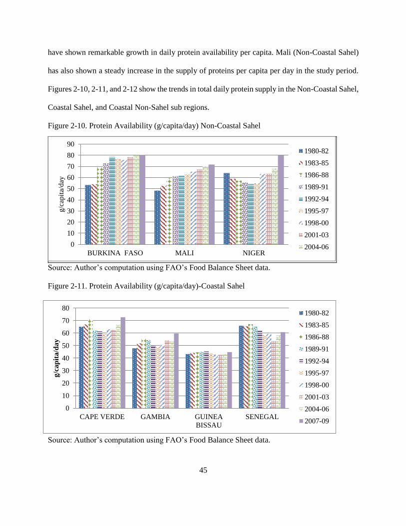
45
have shown remarkable growth in daily protein availability per capita. Mali (Non-Coastal Sahel)
has also shown a steady increase in the supply of proteins per capita per day in the study period.
Figures 2-10, 2-11, and 2-12 show the trends in total daily protein supply in the Non-Coastal Sahel,
Coastal Sahel, and Coastal Non-Sahel sub regions.
Figure 2-10. Protein Availability (g/capita/day) Non-Coastal Sahel
Source: Author’s computation using FAO’s Food Balance Sheet data.
Figure 2-11. Protein Availability (g/capita/day)-Coastal Sahel
Source: Author’s computation using FAO’s Food Balance Sheet data.
0
10
20
30
40
50
60
70
80
90
BURKINA FASO MALI NIGER
g/c
apit
a/day
1980-82
1983-85
1986-88
1989-91
1992-94
1995-97
1998-00
2001-03
2004-06
0
10
20
30
40
50
60
70
80
CAPE VERDE GAMBIA GUINEA
BISSAU
SENEGAL
g/c
ap
ita/d
ay
1980-82
1983-85
1986-88
1989-91
1992-94
1995-97
1998-00
2001-03
2004-06
2007-09
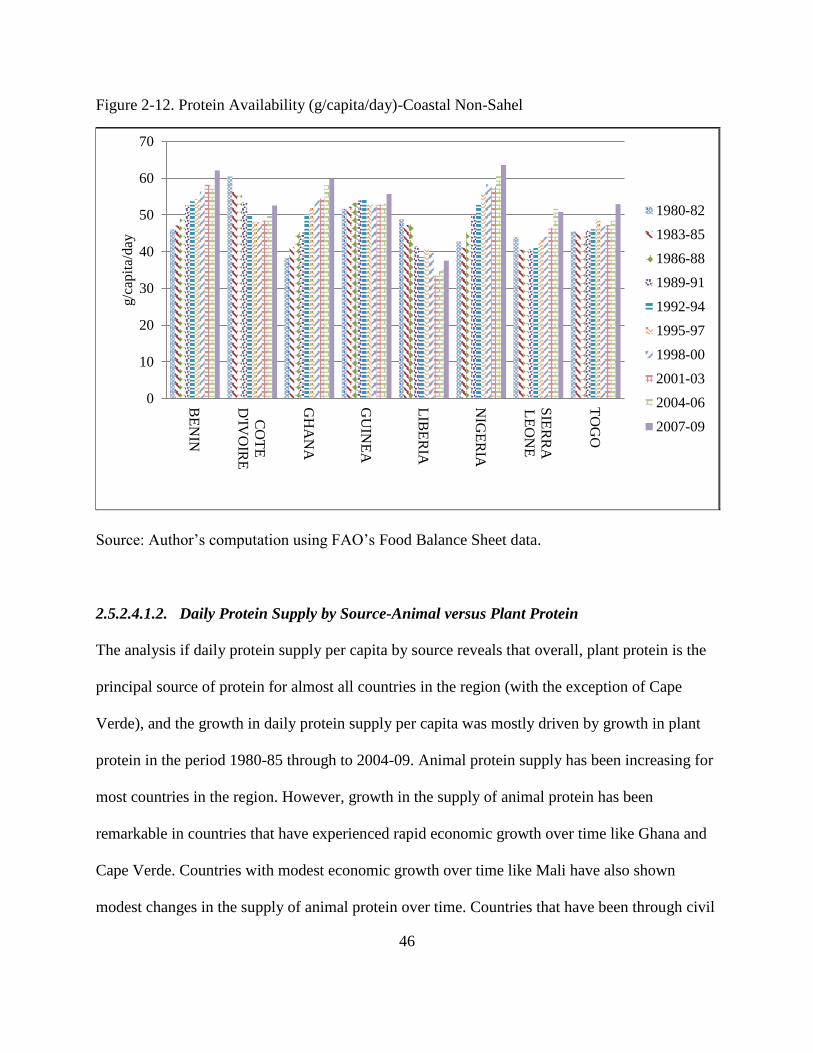
46
Figure 2-12. Protein Availability (g/capita/day)-Coastal Non-Sahel
Source: Author’s computation using FAO’s Food Balance Sheet data.
2.5.2.4.1.2. Daily Protein Supply by Source-Animal versus Plant Protein
The analysis if daily protein supply per capita by source reveals that overall, plant protein is the
principal source of protein for almost all countries in the region (with the exception of Cape
Verde), and the growth in daily protein supply per capita was mostly driven by growth in plant
protein in the period 1980-85 through to 2004-09. Animal protein supply has been increasing for
most countries in the region. However, growth in the supply of animal protein has been
remarkable in countries that have experienced rapid economic growth over time like Ghana and
Cape Verde. Countries with modest economic growth over time like Mali have also shown
modest changes in the supply of animal protein over time. Countries that have been through civil
0
10
20
30
40
50
60
70
BE
NIN
CO
TE
D'IV
OIR
E
GH
AN
A
GU
INE
A
LIB
ER
IA
NIG
ER
IA
SIE
RR
A
LE
ON
E
TO
GO
g/c
apit
a/d
ay
1980-82
1983-85
1986-88
1989-91
1992-94
1995-97
1998-00
2001-03
2004-06
2007-09
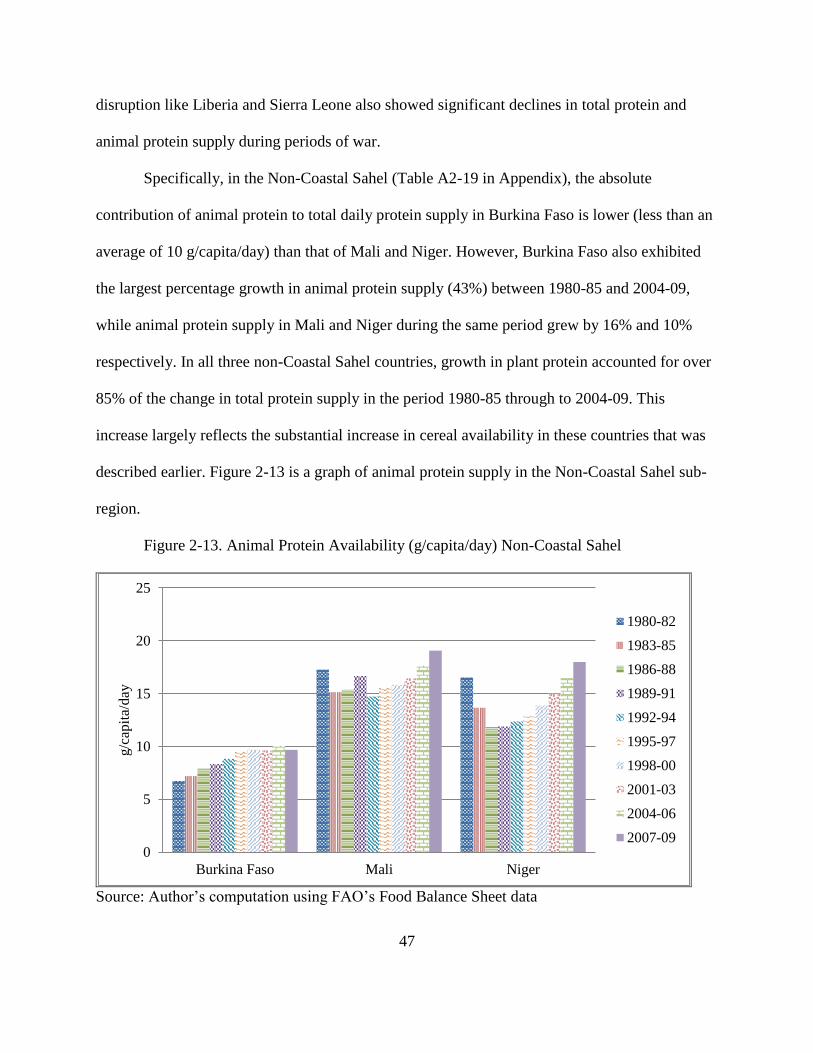
47
disruption like Liberia and Sierra Leone also showed significant declines in total protein and
animal protein supply during periods of war.
Specifically, in the Non-Coastal Sahel (Table A2-19 in Appendix), the absolute
contribution of animal protein to total daily protein supply in Burkina Faso is lower (less than an
average of 10 g/capita/day) than that of Mali and Niger. However, Burkina Faso also exhibited
the largest percentage growth in animal protein supply (43%) between 1980-85 and 2004-09,
while animal protein supply in Mali and Niger during the same period grew by 16% and 10%
respectively. In all three non-Coastal Sahel countries, growth in plant protein accounted for over
85% of the change in total protein supply in the period 1980-85 through to 2004-09. This
increase largely reflects the substantial increase in cereal availability in these countries that was
described earlier. Figure 2-13 is a graph of animal protein supply in the Non-Coastal Sahel sub-
region.
Figure 2-13. Animal Protein Availability (g/capita/day) Non-Coastal Sahel
Source: Author’s computation using FAO’s Food Balance Sheet data
0
5
10
15
20
25
Burkina Faso Mali Niger
g/c
apit
a/day
1980-82
1983-85
1986-88
1989-91
1992-94
1995-97
1998-00
2001-03
2004-06
2007-09
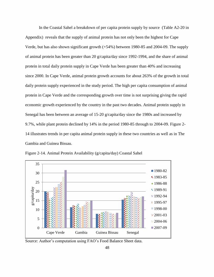
48
In the Coastal Sahel a breakdown of per capita protein supply by source (Table A2-20 in
Appendix) reveals that the supply of animal protein has not only been the highest for Cape
Verde, but has also shown significant growth (+54%) between 1980-85 and 2004-09. The supply
of animal protein has been greater than 20 g/capita/day since 1992-1994, and the share of animal
protein in total daily protein supply in Cape Verde has been greater than 40% and increasing
since 2000. In Cape Verde, animal protein growth accounts for about 263% of the growth in total
daily protein supply experienced in the study period. The high per capita consumption of animal
protein in Cape Verde and the corresponding growth over time is not surprising giving the rapid
economic growth experienced by the country in the past two decades. Animal protein supply in
Senegal has been between an average of 15-20 g/capita/day since the 1980s and increased by
9.7%, while plant protein declined by 14% in the period 1980-85 through to 2004-09. Figure 2-
14 illustrates trends in per capita animal protein supply in these two countries as well as in The
Gambia and Guinea Bissau.
Figure 2-14. Animal Protein Availability (g/capita/day) Coastal Sahel
Source: Author’s computation using FAO’s Food Balance Sheet data.
0
5
10
15
20
25
30
35
Cape Verde Gambia Guinea Bissau Senegal
g/c
apit
a/d
ay
1980-82
1983-85
1986-88
1989-91
1992-94
1995-97
1998-00
2001-03
2004-06
2007-09
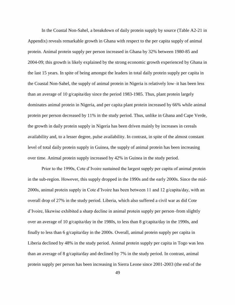
49
In the Coastal Non-Sahel, a breakdown of daily protein supply by source (Table A2-21 in
Appendix) reveals remarkable growth in Ghana with respect to the per capita supply of animal
protein. Animal protein supply per person increased in Ghana by 32% between 1980-85 and
2004-09; this growth is likely explained by the strong economic growth experienced by Ghana in
the last 15 years. In spite of being amongst the leaders in total daily protein supply per capita in
the Coastal Non-Sahel, the supply of animal protein in Nigeria is relatively low–it has been less
than an average of 10 g/capita/day since the period 1983-1985. Thus, plant protein largely
dominates animal protein in Nigeria, and per capita plant protein increased by 66% while animal
protein per person decreased by 11% in the study period. Thus, unlike in Ghana and Cape Verde,
the growth in daily protein supply in Nigeria has been driven mainly by increases in cereals
availability and, to a lesser degree, pulse availability. In contrast, in spite of the almost constant
level of total daily protein supply in Guinea, the supply of animal protein has been increasing
over time. Animal protein supply increased by 42% in Guinea in the study period.
Prior to the 1990s, Cote d’Ivoire sustained the largest supply per capita of animal protein
in the sub-region. However, this supply dropped in the 1990s and the early 2000s. Since the mid-
2000s, animal protein supply in Cote d’Ivoire has been between 11 and 12 g/capita/day, with an
overall drop of 27% in the study period. Liberia, which also suffered a civil war as did Cote
d’Ivoire, likewise exhibited a sharp decline in animal protein supply per person–from slightly
over an average of 10 g/capita/day in the 1980s, to less than 8 g/capita/day in the 1990s, and
finally to less than 6 g/capita/day in the 2000s. Overall, animal protein supply per capita in
Liberia declined by 48% in the study period. Animal protein supply per capita in Togo was less
than an average of 8 g/capita/day and declined by 7% in the study period. In contrast, animal
protein supply per person has been increasing in Sierra Leone since 2001-2003 (the end of the
50
country’s civil war), with an overall increase of 28% in the study period. With the exception of
Cote d’Ivoire, Guinea, and Liberia in the Coastal Non-Sahel region, more than 75% of the
change in total daily supply of protein per person is accounted for by the growth in plant protein
supply. Figure 2-15 shows the trend in animal protein availability per capita in the Coastal non-
Sahel.
Figure 2-15. Animal Protein Availability (g/capita/day) Coastal Non-Sahel
Source: Author’s computation using FAO’sFood Balance Sheet data
0
2
4
6
8
10
12
14
16
18
20
Benin Cote
d'Ivoire
Ghana Guinea Liberia Nigeria Sierra
Leone
Togo
g/c
apit
a/day
1980-82
1983-85
1986-88
1989-91
1992-94
1995-97
1998-00
2001-03
2004-06
2007-09
51
2.5.2.4.1.3. Animal Protein by Source
Overall, a disaggregation of animal protein by specific source (meats, fish and seafood, eggs, and
milk) revealed some interesting trends across all countries in the region. To ensure
comparability, the supply of milk reported in FAOSTAT is converted20 to its dry milk
equivalent given that fluid milk has a high water content. Particularly, the rate of growth in
poultry meat supply per capita has been quite large for most countries in the region–from 45% in
Togo to 1246% in Cape Verde, in the period 1980-85 through to 2004-09. In Benin, for instance,
poultry meat supply per capita and milk increased at the expense of all other sources of animal
protein, indicating some level of substitution. However, in the Coastal Non-Sahel, fish and
seafood remains the most important animal protein source in spite of the increase in poultry meat
availability. In Guinea and Sierra Leone, fish and seafood supply per capita grew in the study
period. Fish and seafood supply per capita also increased in Niger and Mali (Non-Coastal Sahel),
and Senegal and the Gambia (Coastal Sahel). In the Gambia, poultry meat, fish, and seafood and,
to a small extent, eggs are substituting for all other sources of animal protein.
Empirical data for the Non-Coastal Sahel reveals that over time, beef, mutton, and goat
meat have been the major sources of meat in the Non-Coastal Sahel region.
In Burkina Faso (Table 2-3), in the study period, per capita supply of beef increased by 4 kg/year
(109%); that of mutton and goat meat increased by 1 kg/year (35%); that of pig meat by 2
kg/year (about 357%, albeit from a very low base); that of poultry meat by 49%; that of fish and
20 Conversion factor is 10%, i.e., dry milk equals fluid milk divided by 10.
52
seafood by 15%; and that of eggs increased by 1 kg/capita (about 100%). Milk supply in dry
milk equivalent decreased by 1 kg (29%) in Burkina Faso in the study period.
In Mali (Table 2-4), poultry meat supply grew the most in percentage terms (50%) in the
study period but still remains well below the supply of beef, mutton and goat meat. Fish and
seafood supply is largest for Mali in the Non-Coastal Sahel region, and has been fairly stable
over time. Milk supply in Mali increased by 1 kg (13%) in the period 1980-85 through to 2004-
09. Egg supply per capita was below 1 kg/year in the study period. In Niger (Table 2-5), beef
supply per capita experienced the largest absolute increase–5 kg/year (56%) in the period 1980-
85 through to 2004-09. Per capita consumption of fish and seafood also grew by 2 kg/year
(218%), while that of poultry meat dropped by 40%.
53
Table 2-3. Three-Year Averages of Animal Protein Supply (kg/capita) in Non-Coastal Sahel- Burkina Faso
1980
to
1982
1983
to
1985
1986
to
1988
1989
to
1991
1992
to
1994
1995
to
1997
1998
to
2000
2001
to
2003
2004
to
2006
2007
to
2009
% change
1980-85
to
2004-09
CAGR
1980/85
to
2005/09
Bovine Meat 3.2 3.9 4.4 5.7 6.4 6.8 7.1 7.4 7.7 7.2 109.30% 3.0%
Mutton & Goat
Meat 2.1 2.6 2.8 3.2 3.3 3.3 3.3 3.3 3.2 3.1 34.80% 1.2%
Pigmeat 0.4 0.6 0.7 0.8 1.1 1.3 1.6 2 2.4 2.2 356.70% 6.3%
Poultry Meat 1.4 1.6 2 2.2 2.2 2.2 2.2 2.3 2.2 2.2 49.40% 1.5%
Meat, Other 0.9 0.9 0.9 0.8 0.7 0.7 0.6 0.6 0.6 0.6 -34.50% -1.6%
Fish & Seafood 2 2 2 2 2 2 2 2 2 2 0.6%
Eggs 1 1 1 2 3 3 2 2 2 2 100% 2.8%
Milk - dry
equivalent 2.6 2.2 2.3 1.6 1.6 1.7 1.8 1.6 1.7 1.7 -29% -1.4%
Source: Author's calculations using FAO’s Food Balance Sheet data.
54
Table 2-4. Three-Year Averages of Animal Protein Supply (kg/capita) in Non-Coastal Sahel - Mali
1980
to
1982
1983
to
1985
1986
to
1988
1989
to
1991
1992
to
1994
1995
to
1997
1998
to
2000
2001
to
2003
2004
to
2006
2007
to
2009
% change
1980-85
to
2004-09
CAGR
1980/85
to
2005/09
Bovine Meat 5.8 6.7 7.8 8.3 6.0 6.1 6.6 7.4 8.2 9.0 37% 1.3%
Mutton and Goat
Meat
6.5 4.7 4.2 4.9 4.3 4.5 4.8 5.1 5.5 6.9 10% 0.4%
Pig Meat 0.2 0.2 0.2 0.2 0.2 0.2 0.2 0.2 0.2 0.2 8% 0.0%
Poultry Meat 1.7 2.2 2.8 2.7 2.7 2.6 2.8 2.8 3.1 2.8 50% 1.7%
Meat, Other 3.3 2.9 2.7 2.6 2.4 2.4 2.5 2.6 2.9 2.9 -7% -0.3%
Fish and Seafood 10.2 7.3 7.1 8.3 7.2 11.3 9.4 9.1 9.0 8.1 -2% 0.0%
Eggs 0.6 0.7 0.9 0.8 0.8 0.7 0.6 0.5 0.4 0.5 -37% -1.8%
Milk - dry equiv. 5.9 4.7 4.6 5.1 5.1 4.8 5.2 5.2 5.7 6.3 13% 0.5%
Source: Author’s computation using FAO’s Food Balance Sheet data.
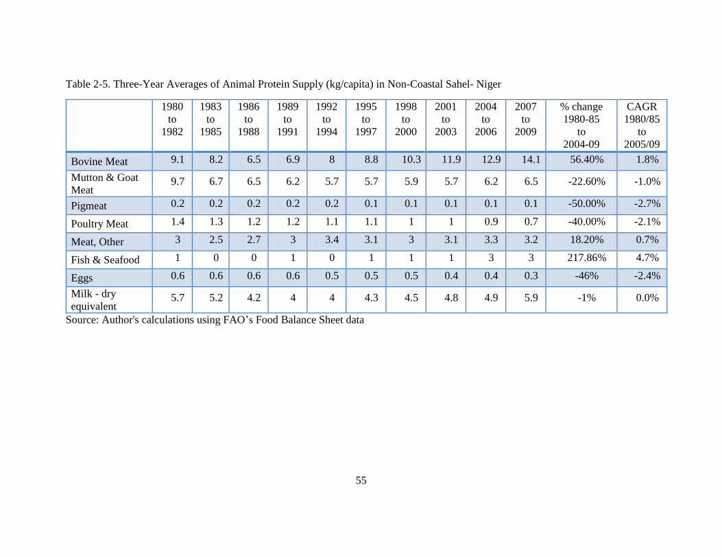
55
Table 2-5. Three-Year Averages of Animal Protein Supply (kg/capita) in Non-Coastal Sahel- Niger
1980
to
1982
1983
to
1985
1986
to
1988
1989
to
1991
1992
to
1994
1995
to
1997
1998
to
2000
2001
to
2003
2004
to
2006
2007
to
2009
% change
1980-85
to
2004-09
CAGR
1980/85
to
2005/09
Bovine Meat 9.1 8.2 6.5 6.9 8 8.8 10.3 11.9 12.9 14.1 56.40% 1.8%
Mutton & Goat
Meat 9.7 6.7 6.5 6.2 5.7 5.7 5.9 5.7 6.2 6.5 -22.60% -1.0%
Pigmeat 0.2 0.2 0.2 0.2 0.2 0.1 0.1 0.1 0.1 0.1 -50.00% -2.7%
Poultry Meat 1.4 1.3 1.2 1.2 1.1 1.1 1 1 0.9 0.7 -40.00% -2.1%
Meat, Other 3 2.5 2.7 3 3.4 3.1 3 3.1 3.3 3.2 18.20% 0.7%
Fish & Seafood 1 0 0 1 0 1 1 1 3 3 217.86% 4.7%
Eggs 0.6 0.6 0.6 0.6 0.5 0.5 0.5 0.4 0.4 0.3 -46% -2.4%
Milk - dry
equivalent 5.7 5.2 4.2 4 4 4.3 4.5 4.8 4.9 5.9 -1% 0.0%
Source: Author's calculations using FAO’s Food Balance Sheet data
56
In the Coastal Sahel (Table 2-6) there was huge growth in the supply of poultry meat in
the period 1980-85 and 2004-09. Poultry meat supply per capita increased by 1,246% in Cape
Verde; 455% in The Gambia; 256% in Guinea Bissau; and 101% in Senegal in the study period. Pig
meat has been the dominant source of meat over time in Cape Verde, and its supply per person also
increased by about 290% in the study period. Unlike pig meat, most of the increase in Cape Verde’s
poultry meat was imported. Poultry meat supply from imports increased from less than 1,000 tons
prior to 2000 to an average of 8,000 tons in the period 2007-09. In spite of the high per capita
availability of fish and seafood in Cape Verde in the early and mid-1980s, per capita availability
dropped by 59% in the study period as chicken apparently substituted for fish in consumption. Per
capita supply of eggs also increased by 3 kg (an increase of 300%) while that dry milk also
increased by about 5 kg (an increase of about 69%) in Cape Verde in the study period.
In Senegal and The Gambia, beef dominated in meat supply over time. However, its per
capita supply declined over time in both countries. Pig meat is the dominant source of meat in
Guinea Bissau (in spite of a 14% decline in per capita supply over time). The fish and seafood
supply in Senegal grew from an average of 22 kg/person/year in the period 1980-85 to 25
kg/person/year.
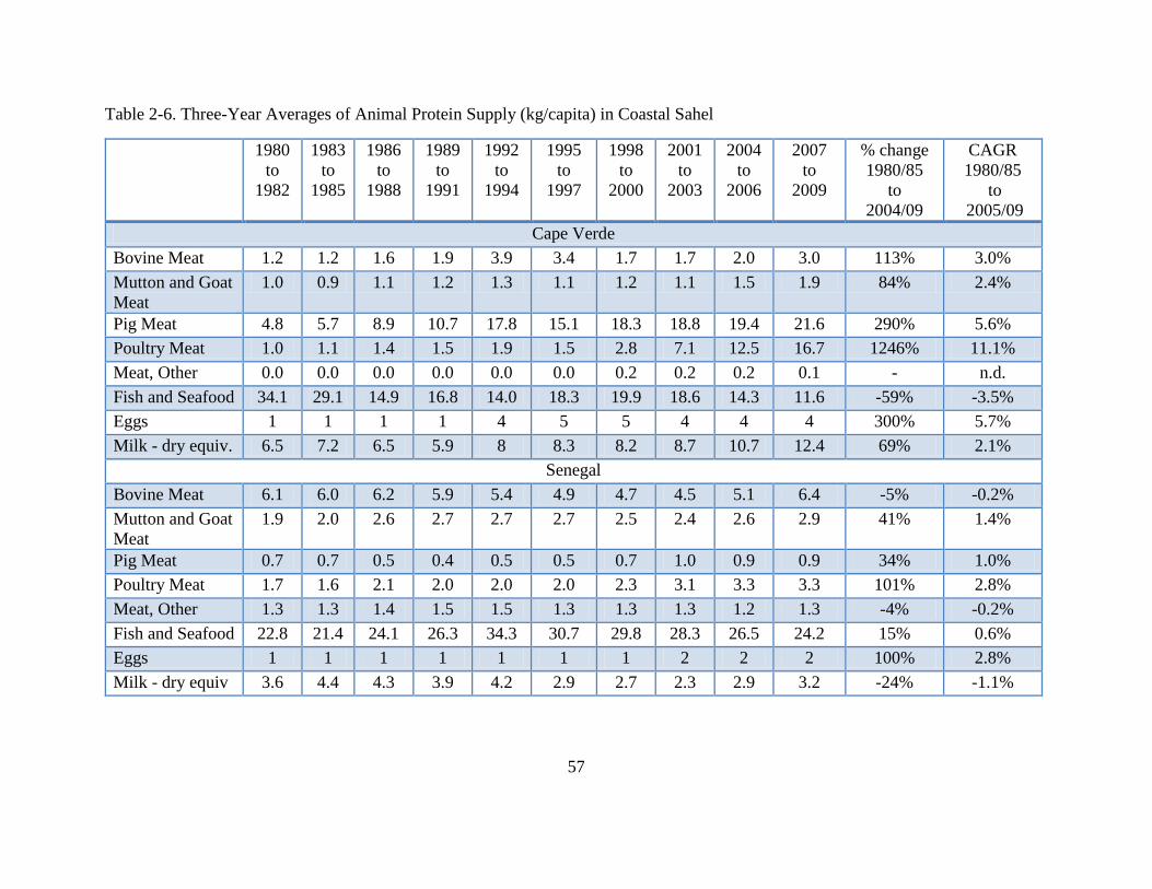
57
Table 2-6. Three-Year Averages of Animal Protein Supply (kg/capita) in Coastal Sahel
1980
to
1982
1983
to
1985
1986
to
1988
1989
to
1991
1992
to
1994
1995
to
1997
1998
to
2000
2001
to
2003
2004
to
2006
2007
to
2009
% change
1980/85
to
2004/09
CAGR
1980/85
to
2005/09
Cape Verde
Bovine Meat 1.2 1.2 1.6 1.9 3.9 3.4 1.7 1.7 2.0 3.0 113% 3.0%
Mutton and Goat
Meat
1.0 0.9 1.1 1.2 1.3 1.1 1.2 1.1 1.5 1.9 84% 2.4%
Pig Meat 4.8 5.7 8.9 10.7 17.8 15.1 18.3 18.8 19.4 21.6 290% 5.6%
Poultry Meat 1.0 1.1 1.4 1.5 1.9 1.5 2.8 7.1 12.5 16.7 1246% 11.1%
Meat, Other 0.0 0.0 0.0 0.0 0.0 0.0 0.2 0.2 0.2 0.1 - n.d.
Fish and Seafood 34.1 29.1 14.9 16.8 14.0 18.3 19.9 18.6 14.3 11.6 -59% -3.5%
Eggs 1 1 1 1 4 5 5 4 4 4 300% 5.7%
Milk - dry equiv. 6.5 7.2 6.5 5.9 8 8.3 8.2 8.7 10.7 12.4 69% 2.1%
Senegal
Bovine Meat 6.1 6.0 6.2 5.9 5.4 4.9 4.7 4.5 5.1 6.4 -5% -0.2%
Mutton and Goat
Meat
1.9 2.0 2.6 2.7 2.7 2.7 2.5 2.4 2.6 2.9 41% 1.4%
Pig Meat 0.7 0.7 0.5 0.4 0.5 0.5 0.7 1.0 0.9 0.9 34% 1.0%
Poultry Meat 1.7 1.6 2.1 2.0 2.0 2.0 2.3 3.1 3.3 3.3 101% 2.8%
Meat, Other 1.3 1.3 1.4 1.5 1.5 1.3 1.3 1.3 1.2 1.3 -4% -0.2%
Fish and Seafood 22.8 21.4 24.1 26.3 34.3 30.7 29.8 28.3 26.5 24.2 15% 0.6%
Eggs 1 1 1 1 1 1 1 2 2 2 100% 2.8%
Milk - dry equiv 3.6 4.4 4.3 3.9 4.2 2.9 2.7 2.3 2.9 3.2 -24% -1.1%
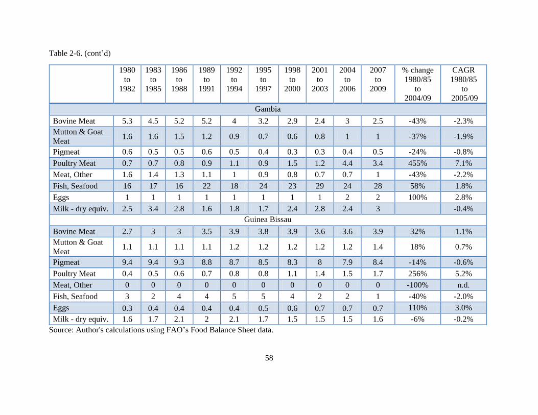
58
Table 2-6. (cont’d)
1980
to
1982
1983
to
1985
1986
to
1988
1989
to
1991
1992
to
1994
1995
to
1997
1998
to
2000
2001
to
2003
2004
to
2006
2007
to
2009
% change
1980/85
to
2004/09
CAGR
1980/85
to
2005/09
Gambia
Bovine Meat 5.3 4.5 5.2 5.2 4 3.2 2.9 2.4 3 2.5 -43% -2.3%
Mutton & Goat
Meat 1.6 1.6 1.5 1.2 0.9 0.7 0.6 0.8 1 1 -37% -1.9%
Pigmeat 0.6 0.5 0.5 0.6 0.5 0.4 0.3 0.3 0.4 0.5 -24% -0.8%
Poultry Meat 0.7 0.7 0.8 0.9 1.1 0.9 1.5 1.2 4.4 3.4 455% 7.1%
Meat, Other 1.6 1.4 1.3 1.1 1 0.9 0.8 0.7 0.7 1 -43% -2.2%
Fish, Seafood 16 17 16 22 18 24 23 29 24 28 58% 1.8%
Eggs 1 1 1 1 1 1 1 1 2 2 100% 2.8%
Milk - dry equiv. 2.5 3.4 2.8 1.6 1.8 1.7 2.4 2.8 2.4 3 -0.4%
Guinea Bissau
Bovine Meat 2.7 3 3 3.5 3.9 3.8 3.9 3.6 3.6 3.9 32% 1.1%
Mutton & Goat
Meat 1.1 1.1 1.1 1.1 1.2 1.2 1.2 1.2 1.2 1.4 18% 0.7%
Pigmeat 9.4 9.4 9.3 8.8 8.7 8.5 8.3 8 7.9 8.4 -14% -0.6%
Poultry Meat 0.4 0.5 0.6 0.7 0.8 0.8 1.1 1.4 1.5 1.7 256% 5.2%
Meat, Other 0 0 0 0 0 0 0 0 0 0 -100% n.d.
Fish, Seafood 3 2 4 4 5 5 4 2 2 1 -40% -2.0%
Eggs 0.3 0.4 0.4 0.4 0.4 0.5 0.6 0.7 0.7 0.7 110% 3.0%
Milk - dry equiv. 1.6 1.7 2.1 2 2.1 1.7 1.5 1.5 1.5 1.6 -6% -0.2%
Source: Author's calculations using FAO’s Food Balance Sheet data.
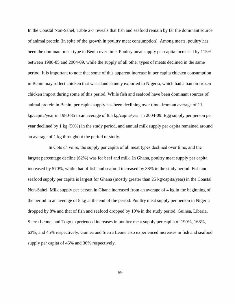
59
In the Coastal Non-Sahel, Table 2-7 reveals that fish and seafood remain by far the dominant source
of animal protein (in spite of the growth in poultry meat consumption). Among meats, poultry has
been the dominant meat type in Benin over time. Poultry meat supply per capita increased by 115%
between 1980-85 and 2004-09, while the supply of all other types of meats declined in the same
period. It is important to note that some of this apparent increase in per capita chicken consumption
in Benin may reflect chicken that was clandestinely exported to Nigeria, which had a ban on frozen
chicken import during some of this period. While fish and seafood have been dominant sources of
animal protein in Benin, per capita supply has been declining over time–from an average of 11
kg/capita/year in 1980-85 to an average of 8.5 kg/capita/year in 2004-09. Egg supply per person per
year declined by 1 kg (50%) in the study period, and annual milk supply per capita remained around
an average of 1 kg throughout the period of study.
In Cote d’Ivoire, the supply per capita of all meat types declined over time, and the
largest percentage decline (62%) was for beef and milk. In Ghana, poultry meat supply per capita
increased by 570%, while that of fish and seafood increased by 38% in the study period. Fish and
seafood supply per capita is largest for Ghana (mostly greater than 25 kg/capita/year) in the Coastal
Non-Sahel. Milk supply per person in Ghana increased from an average of 4 kg in the beginning of
the period to an average of 8 kg at the end of the period. Poultry meat supply per person in Nigeria
dropped by 8% and that of fish and seafood dropped by 10% in the study period. Guinea, Liberia,
Sierra Leone, and Togo experienced increases in poultry meat supply per capita of 190%, 168%,
63%, and 45% respectively. Guinea and Sierra Leone also experienced increases in fish and seafood
supply per capita of 45% and 36% respectively.
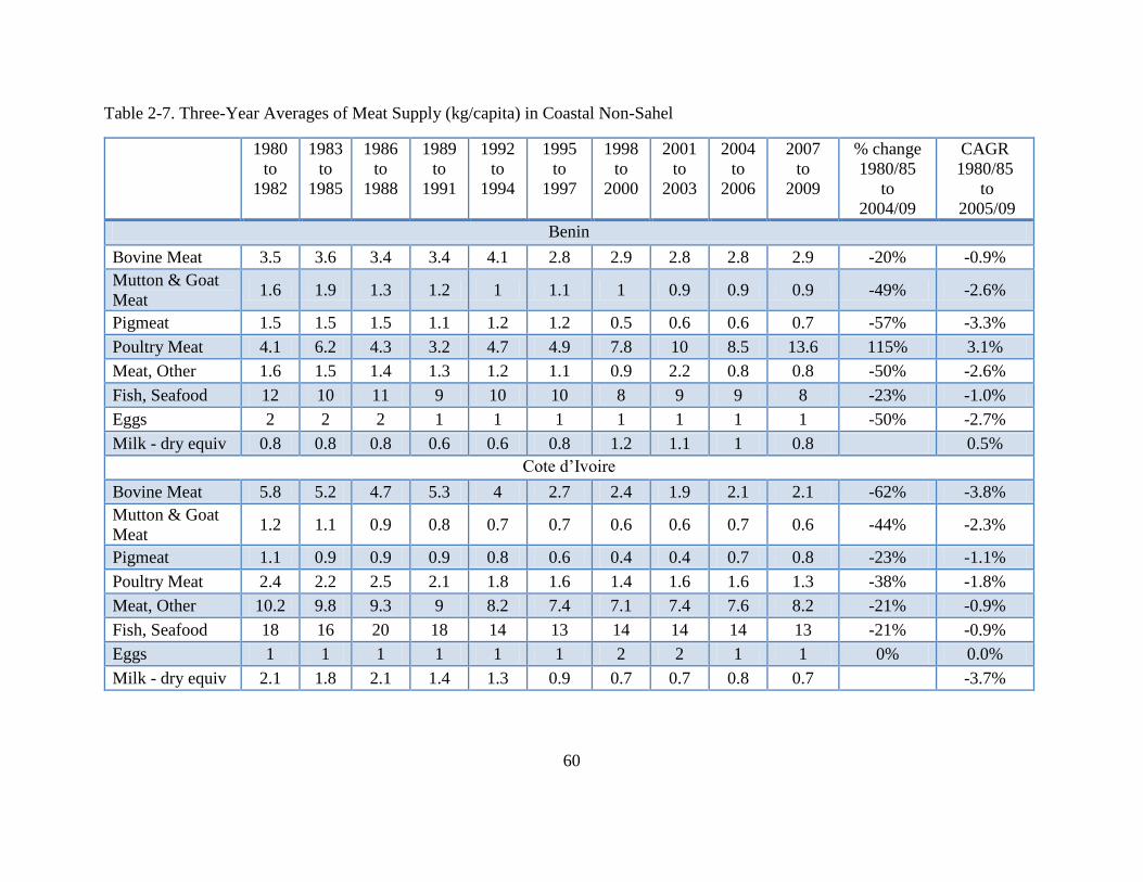
60
Table 2-7. Three-Year Averages of Meat Supply (kg/capita) in Coastal Non-Sahel
1980
to
1982
1983
to
1985
1986
to
1988
1989
to
1991
1992
to
1994
1995
to
1997
1998
to
2000
2001
to
2003
2004
to
2006
2007
to
2009
% change
1980/85
to
2004/09
CAGR
1980/85
to
2005/09
Benin
Bovine Meat 3.5 3.6 3.4 3.4 4.1 2.8 2.9 2.8 2.8 2.9 -20% -0.9%
Mutton & Goat
Meat 1.6 1.9 1.3 1.2 1 1.1 1 0.9 0.9 0.9 -49% -2.6%
Pigmeat 1.5 1.5 1.5 1.1 1.2 1.2 0.5 0.6 0.6 0.7 -57% -3.3%
Poultry Meat 4.1 6.2 4.3 3.2 4.7 4.9 7.8 10 8.5 13.6 115% 3.1%
Meat, Other 1.6 1.5 1.4 1.3 1.2 1.1 0.9 2.2 0.8 0.8 -50% -2.6%
Fish, Seafood 12 10 11 9 10 10 8 9 9 8 -23% -1.0%
Eggs 2 2 2 1 1 1 1 1 1 1 -50% -2.7%
Milk - dry equiv 0.8 0.8 0.8 0.6 0.6 0.8 1.2 1.1 1 0.8 0.5%
Cote d’Ivoire
Bovine Meat 5.8 5.2 4.7 5.3 4 2.7 2.4 1.9 2.1 2.1 -62% -3.8%
Mutton & Goat
Meat 1.2 1.1 0.9 0.8 0.7 0.7 0.6 0.6 0.7 0.6 -44% -2.3%
Pigmeat 1.1 0.9 0.9 0.9 0.8 0.6 0.4 0.4 0.7 0.8 -23% -1.1%
Poultry Meat 2.4 2.2 2.5 2.1 1.8 1.6 1.4 1.6 1.6 1.3 -38% -1.8%
Meat, Other 10.2 9.8 9.3 9 8.2 7.4 7.1 7.4 7.6 8.2 -21% -0.9%
Fish, Seafood 18 16 20 18 14 13 14 14 14 13 -21% -0.9%
Eggs 1 1 1 1 1 1 2 2 1 1 0% 0.0%
Milk - dry equiv 2.1 1.8 2.1 1.4 1.3 0.9 0.7 0.7 0.8 0.7 -3.7%
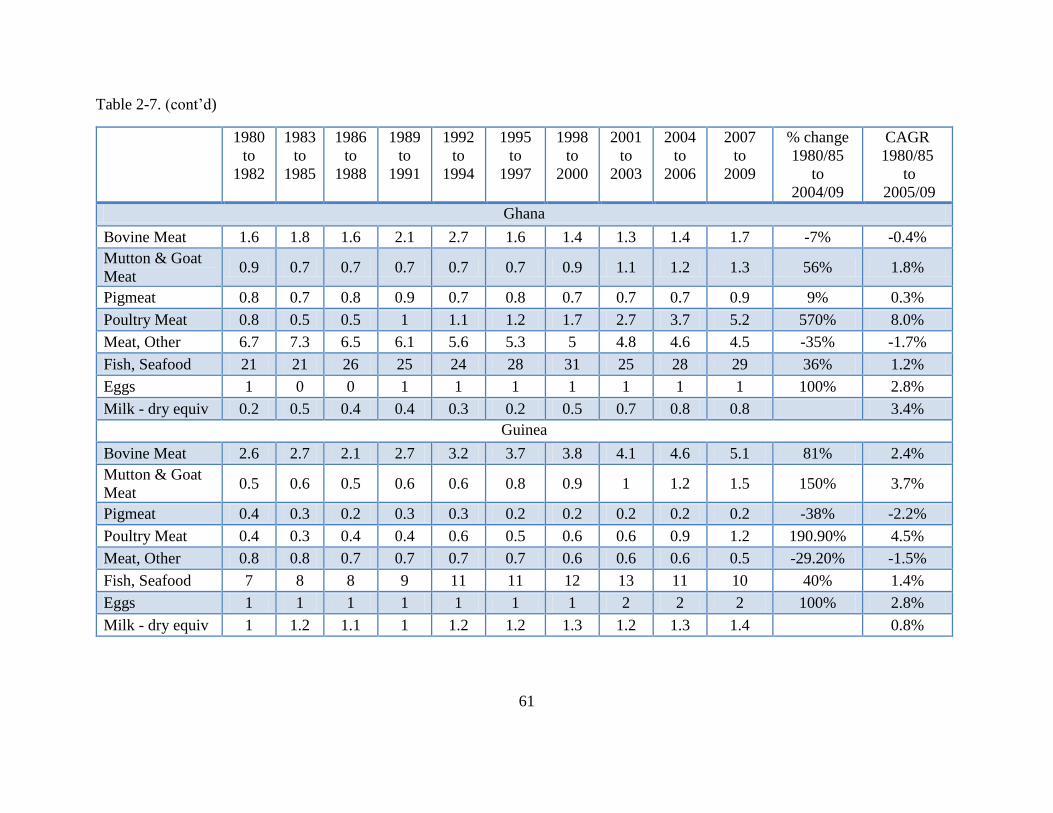
61
Table 2-7. (cont’d)
1980
to
1982
1983
to
1985
1986
to
1988
1989
to
1991
1992
to
1994
1995
to
1997
1998
to
2000
2001
to
2003
2004
to
2006
2007
to
2009
% change
1980/85
to
2004/09
CAGR
1980/85
to
2005/09
Ghana
Bovine Meat 1.6 1.8 1.6 2.1 2.7 1.6 1.4 1.3 1.4 1.7 -7% -0.4%
Mutton & Goat
Meat 0.9 0.7 0.7 0.7 0.7 0.7 0.9 1.1 1.2 1.3 56% 1.8%
Pigmeat 0.8 0.7 0.8 0.9 0.7 0.8 0.7 0.7 0.7 0.9 9% 0.3%
Poultry Meat 0.8 0.5 0.5 1 1.1 1.2 1.7 2.7 3.7 5.2 570% 8.0%
Meat, Other 6.7 7.3 6.5 6.1 5.6 5.3 5 4.8 4.6 4.5 -35% -1.7%
Fish, Seafood 21 21 26 25 24 28 31 25 28 29 36% 1.2%
Eggs 1 0 0 1 1 1 1 1 1 1 100% 2.8%
Milk - dry equiv 0.2 0.5 0.4 0.4 0.3 0.2 0.5 0.7 0.8 0.8 3.4%
Guinea
Bovine Meat 2.6 2.7 2.1 2.7 3.2 3.7 3.8 4.1 4.6 5.1 81% 2.4%
Mutton & Goat
Meat 0.5 0.6 0.5 0.6 0.6 0.8 0.9 1 1.2 1.5 150% 3.7%
Pigmeat 0.4 0.3 0.2 0.3 0.3 0.2 0.2 0.2 0.2 0.2 -38% -2.2%
Poultry Meat 0.4 0.3 0.4 0.4 0.6 0.5 0.6 0.6 0.9 1.2 190.90% 4.5%
Meat, Other 0.8 0.8 0.7 0.7 0.7 0.7 0.6 0.6 0.6 0.5 -29.20% -1.5%
Fish, Seafood 7 8 8 9 11 11 12 13 11 10 40% 1.4%
Eggs 1 1 1 1 1 1 1 2 2 2 100% 2.8%
Milk - dry equiv 1 1.2 1.1 1 1.2 1.2 1.3 1.2 1.3 1.4 0.8%
62
Table 2-7. (cont’d)
1980
to
1982
1983
to
1985
1986
to
1988
1989
to
1991
1992
to
1994
1995
to
1997
1998
to
2000
2001
to
2003
2004
to
2006
2007
to
2009
% change
1980/85
to
2004/09
CAGR
1980/85
to
2005/09
Liberia
Bovine Meat 1.4 1.3 0.9 0.9 1.7 0.7 0.6 0.5 0.4 0.3 -73% -5.3%
Mutton & Goat
Meat 0.6 0.6 0.6 0.6 0.7 0.6 0.5 0.4 0.4 0.5 -28% -1.1%
Pigmeat 2.1 2 2.2 2.3 2.3 2.2 1.9 1.9 2.4 2.6 21% 0.8%
Poultry Meat 1.5 1.8 2.4 2.7 2.9 3.1 3.4 3 4.2 4.6 168% 4.0%
Meat, Other 6.9 6.3 6.7 3.6 3.6 3.6 3.2 2.5 2.2 2.4 -65% -4.1%
Fish, Seafood 13 15 15 10 6 6 6 4 5 5 -64% -4.0%
Eggs 1 2 2 2 2 2 2 1 2 2 33% 1.2%
Milk - dry equiv 1 1.3 0.8 0.4 0.3 0.3 0.3 0.2 0.4 0.3 -4.6%
Nigeria
Bovine Meat 5 5.2 3 2.2 2.3 2.5 2.4 2.2 2 1.9 -62% -3.8%
Mutton & Goat
Meat 1.2 1.4 1.6 1.7 1.8 2.1 2.6 2.8 2.8 2.8 110% 3.1%
Pigmeat 0.5 0.6 1 1.1 1.1 1.2 1.3 1.4 1.4 1.4 158% 3.8%
Poultry Meat 1.8 1.7 1.7 1.8 1.6 1.5 1.4 1.5 1.6 1.6 -8% -0.4%
Meat, Other 1.3 1.2 1.1 1 1 0.9 0.9 0.9 0.9 0.9 -31% -1.3%
Fish, Seafood 16 9 7 10 6 7 7 9 9 13 28% -0.5%
Eggs 3 3 3 3 4 3 3 3 3 4 12% 0.6%
Milk - dry equiv 1.5 0.9 0.5 0.6 0.6 0.6 0.5 0.7 0.8 0.8 -1.6%
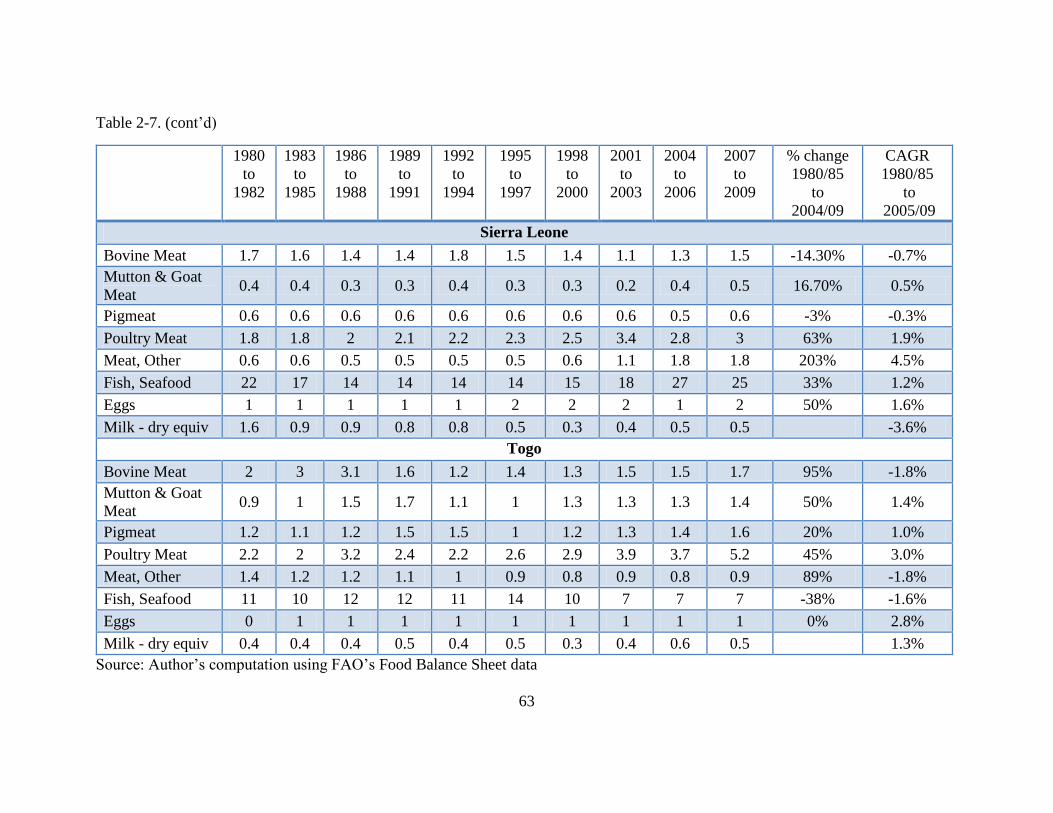
63
Table 2-7. (cont’d)
1980
to
1982
1983
to
1985
1986
to
1988
1989
to
1991
1992
to
1994
1995
to
1997
1998
to
2000
2001
to
2003
2004
to
2006
2007
to
2009
% change
1980/85
to
2004/09
CAGR
1980/85
to
2005/09
Sierra Leone
Bovine Meat 1.7 1.6 1.4 1.4 1.8 1.5 1.4 1.1 1.3 1.5 -14.30% -0.7%
Mutton & Goat
Meat 0.4 0.4 0.3 0.3 0.4 0.3 0.3 0.2 0.4 0.5 16.70% 0.5%
Pigmeat 0.6 0.6 0.6 0.6 0.6 0.6 0.6 0.6 0.5 0.6 -3% -0.3%
Poultry Meat 1.8 1.8 2 2.1 2.2 2.3 2.5 3.4 2.8 3 63% 1.9%
Meat, Other 0.6 0.6 0.5 0.5 0.5 0.5 0.6 1.1 1.8 1.8 203% 4.5%
Fish, Seafood 22 17 14 14 14 14 15 18 27 25 33% 1.2%
Eggs 1 1 1 1 1 2 2 2 1 2 50% 1.6%
Milk - dry equiv 1.6 0.9 0.9 0.8 0.8 0.5 0.3 0.4 0.5 0.5 -3.6%
Togo
Bovine Meat 2 3 3.1 1.6 1.2 1.4 1.3 1.5 1.5 1.7 95% -1.8%
Mutton & Goat
Meat 0.9 1 1.5 1.7 1.1 1 1.3 1.3 1.3 1.4 50% 1.4%
Pigmeat 1.2 1.1 1.2 1.5 1.5 1 1.2 1.3 1.4 1.6 20% 1.0%
Poultry Meat 2.2 2 3.2 2.4 2.2 2.6 2.9 3.9 3.7 5.2 45% 3.0%
Meat, Other 1.4 1.2 1.2 1.1 1 0.9 0.8 0.9 0.8 0.9 89% -1.8%
Fish, Seafood 11 10 12 12 11 14 10 7 7 7 -38% -1.6%
Eggs 0 1 1 1 1 1 1 1 1 1 0% 2.8%
Milk - dry equiv 0.4 0.4 0.4 0.5 0.4 0.5 0.3 0.4 0.6 0.5 1.3%
Source: Author’s computation using FAO’s Food Balance Sheet data
64
2.5.2.4.1.4. Plant Protein by Source
To further examine the quality of protein supplied, plant protein was disaggregated between the
portion due to pulses and all other plant sources. Pulses are an important share of plant protein
supply in Cape Verde, Niger, and Nigeria. Pulses have accounted for 9% (Burkina Faso) to 57%
(Niger) of the change in plant protein supply in the period 1980-85 through to 2004-09. Compared
to the Non-Coastal Sahel, and with the exception Cape Verde, pulses contribute less than 10
g/capita/day of protein and have had small shares (less than 10%) in daily plant protein supply in
the Coastal Sahel.
In the Coastal Non-Sahel sub-region, protein supply from pulses has been less than 10
g/capita/day, and pulses accounted for from 16% (Nigeria) to 257% (Guinea—from a small base) of
the growth in plant protein in the period of study. The growth in the share of pulses in daily plant
protein supply reflects some degree of diet upgrading. Thus, in spite of the relatively low per capita
availability of high quality animal protein in most countries in the region, the positive growth in
protein supply from pulses as well as in the share of pulses in daily plant protein supply supports
the emergence of pulses as poor people’s meat in the region. Tables 2-8, 2-9, and 2-10 shows the
contribution of pulses to daily plant protein supply per capita in the Non-Coastal Sahel, the Coastal
Sahel and the Coastal Non-Sahel sub regions, respectively.
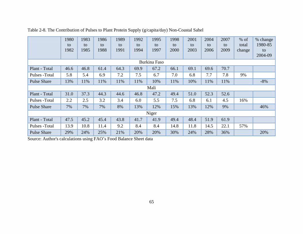
65
Table 2-8. The Contribution of Pulses to Plant Protein Supply (g/capita/day) Non-Coastal Sahel
1980
to
1982
1983
to
1985
1986
to
1988
1989
to
1991
1992
to
1994
1995
to
1997
1998
to
2000
2001
to
2003
2004
to
2006
2007
to
2009
% of
total
change
% change
1980-85
to
2004-09
Burkina Faso
Plant - Total 46.6 46.8 61.4 64.3 69.9 67.2 66.1 69.1 69.6 70.7
Pulses -Total 5.8 5.4 6.9 7.2 7.5 6.7 7.0 6.8 7.7 7.8 9%
Pulse Share 13% 11% 11% 11% 11% 10% 11% 10% 11% 11% -8%
Mali
Plant - Total 31.0 37.3 44.3 44.6 46.8 47.2 49.4 51.0 52.3 52.6
Pulses -Total 2.2 2.5 3.2 3.4 6.0 5.5 7.5 6.8 6.1 4.5 16%
Pulse Share 7% 7% 7% 8% 13% 12% 15% 13% 12% 9% 46%
Niger
Plant - Total 47.5 45.2 45.4 43.8 41.7 41.9 49.4 48.4 51.9 61.9
Pulses -Total 13.9 10.8 11.4 9.2 8.4 8.4 14.8 11.8 14.5 22.1 57%
Pulse Share 29% 24% 25% 21% 20% 20% 30% 24% 28% 36% 20%
Source: Author's calculations using FAO’s Food Balance Sheet data
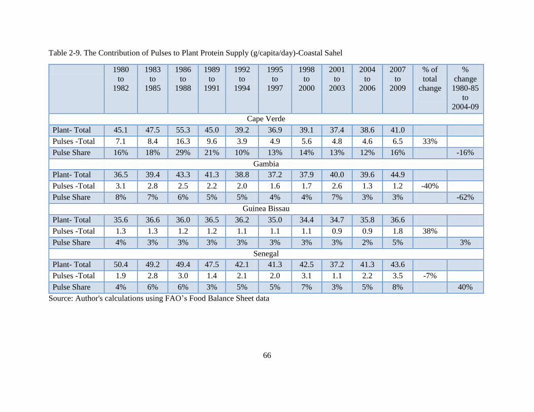
66
Table 2-9. The Contribution of Pulses to Plant Protein Supply (g/capita/day)-Coastal Sahel
1980
to
1982
1983
to
1985
1986
to
1988
1989
to
1991
1992
to
1994
1995
to
1997
1998
to
2000
2001
to
2003
2004
to
2006
2007
to
2009
% of
total
change
%
change
1980-85
to
2004-09
Cape Verde
Plant- Total 45.1 47.5 55.3 45.0 39.2 36.9 39.1 37.4 38.6 41.0
Pulses -Total 7.1 8.4 16.3 9.6 3.9 4.9 5.6 4.8 4.6 6.5 33%
Pulse Share 16% 18% 29% 21% 10% 13% 14% 13% 12% 16% -16%
Gambia
Plant- Total 36.5 39.4 43.3 41.3 38.8 37.2 37.9 40.0 39.6 44.9
Pulses -Total 3.1 2.8 2.5 2.2 2.0 1.6 1.7 2.6 1.3 1.2 -40%
Pulse Share 8% 7% 6% 5% 5% 4% 4% 7% 3% 3% -62%
Guinea Bissau
Plant- Total 35.6 36.6 36.0 36.5 36.2 35.0 34.4 34.7 35.8 36.6
Pulses -Total 1.3 1.3 1.2 1.2 1.1 1.1 1.1 0.9 0.9 1.8 38%
Pulse Share 4% 3% 3% 3% 3% 3% 3% 3% 2% 5% 3%
Senegal
Plant- Total 50.4 49.2 49.4 47.5 42.1 41.3 42.5 37.2 41.3 43.6
Pulses -Total 1.9 2.8 3.0 1.4 2.1 2.0 3.1 1.1 2.2 3.5 -7%
Pulse Share 4% 6% 6% 3% 5% 5% 7% 3% 5% 8% 40%
Source: Author's calculations using FAO’s Food Balance Sheet data
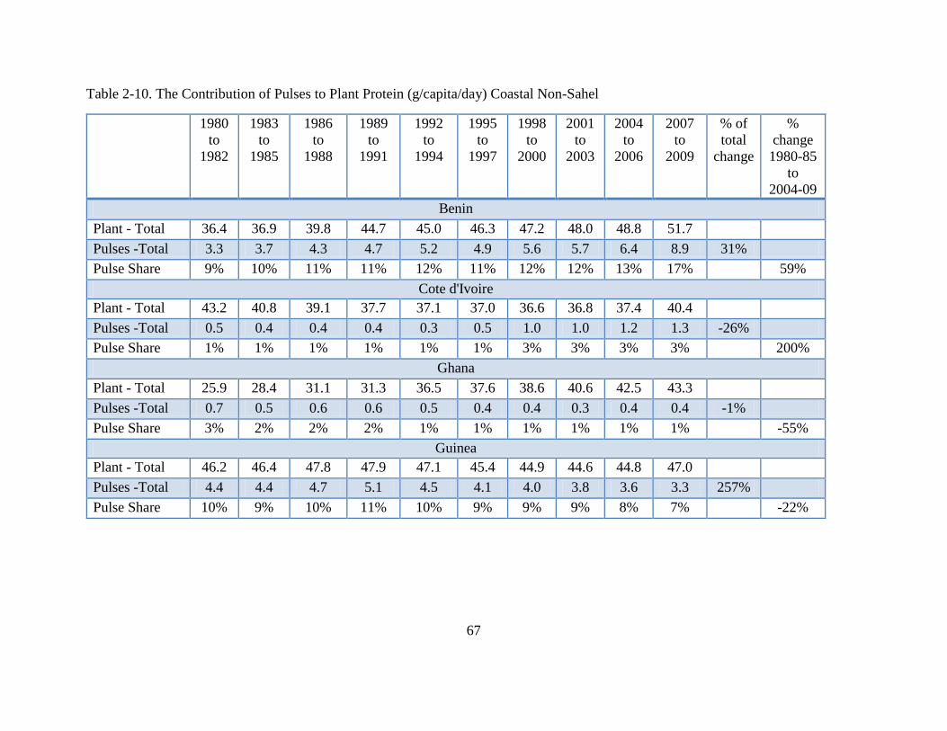
67
Table 2-10. The Contribution of Pulses to Plant Protein (g/capita/day) Coastal Non-Sahel
1980
to
1982
1983
to
1985
1986
to
1988
1989
to
1991
1992
to
1994
1995
to
1997
1998
to
2000
2001
to
2003
2004
to
2006
2007
to
2009
% of
total
change
%
change
1980-85
to
2004-09
Benin
Plant - Total 36.4 36.9 39.8 44.7 45.0 46.3 47.2 48.0 48.8 51.7
Pulses -Total 3.3 3.7 4.3 4.7 5.2 4.9 5.6 5.7 6.4 8.9 31%
Pulse Share 9% 10% 11% 11% 12% 11% 12% 12% 13% 17% 59%
Cote d'Ivoire
Plant - Total 43.2 40.8 39.1 37.7 37.1 37.0 36.6 36.8 37.4 40.4
Pulses -Total 0.5 0.4 0.4 0.4 0.3 0.5 1.0 1.0 1.2 1.3 -26%
Pulse Share 1% 1% 1% 1% 1% 1% 3% 3% 3% 3% 200%
Ghana
Plant - Total 25.9 28.4 31.1 31.3 36.5 37.6 38.6 40.6 42.5 43.3
Pulses -Total 0.7 0.5 0.6 0.6 0.5 0.4 0.4 0.3 0.4 0.4 -1%
Pulse Share 3% 2% 2% 2% 1% 1% 1% 1% 1% 1% -55%
Guinea
Plant - Total 46.2 46.4 47.8 47.9 47.1 45.4 44.9 44.6 44.8 47.0
Pulses -Total 4.4 4.4 4.7 5.1 4.5 4.1 4.0 3.8 3.6 3.3 257%
Pulse Share 10% 9% 10% 11% 10% 9% 9% 9% 8% 7% -22%
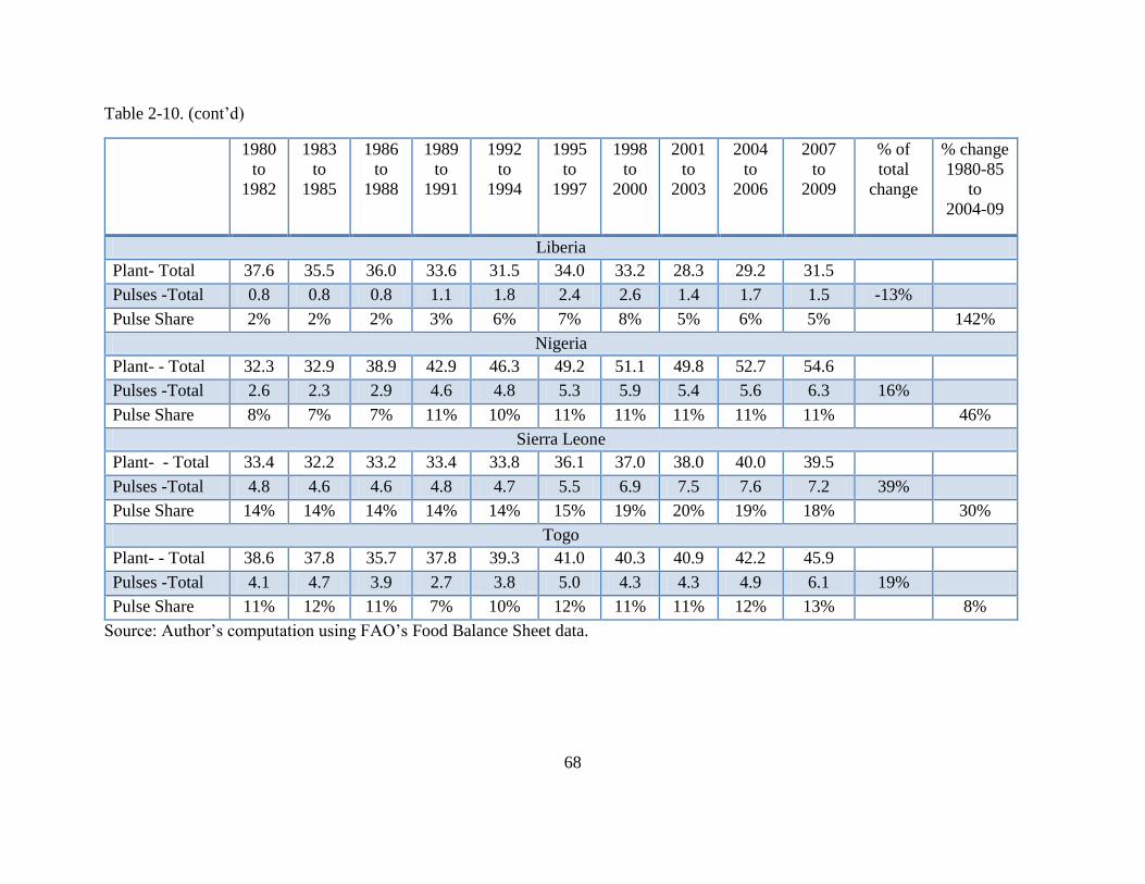
68
Table 2-10. (cont’d)
1980
to
1982
1983
to
1985
1986
to
1988
1989
to
1991
1992
to
1994
1995
to
1997
1998
to
2000
2001
to
2003
2004
to
2006
2007
to
2009
% of
total
change
% change
1980-85
to
2004-09
Liberia
Plant- Total 37.6 35.5 36.0 33.6 31.5 34.0 33.2 28.3 29.2 31.5
Pulses -Total 0.8 0.8 0.8 1.1 1.8 2.4 2.6 1.4 1.7 1.5 -13%
Pulse Share 2% 2% 2% 3% 6% 7% 8% 5% 6% 5% 142%
Nigeria
Plant- - Total 32.3 32.9 38.9 42.9 46.3 49.2 51.1 49.8 52.7 54.6
Pulses -Total 2.6 2.3 2.9 4.6 4.8 5.3 5.9 5.4 5.6 6.3 16%
Pulse Share 8% 7% 7% 11% 10% 11% 11% 11% 11% 11% 46%
Sierra Leone
Plant- - Total 33.4 32.2 33.2 33.4 33.8 36.1 37.0 38.0 40.0 39.5
Pulses -Total 4.8 4.6 4.6 4.8 4.7 5.5 6.9 7.5 7.6 7.2 39%
Pulse Share 14% 14% 14% 14% 14% 15% 19% 20% 19% 18% 30%
Togo
Plant- - Total 38.6 37.8 35.7 37.8 39.3 41.0 40.3 40.9 42.2 45.9
Pulses -Total 4.1 4.7 3.9 2.7 3.8 5.0 4.3 4.3 4.9 6.1 19%
Pulse Share 11% 12% 11% 7% 10% 12% 11% 11% 12% 13% 8%
Source: Author’s computation using FAO’s Food Balance Sheet data.
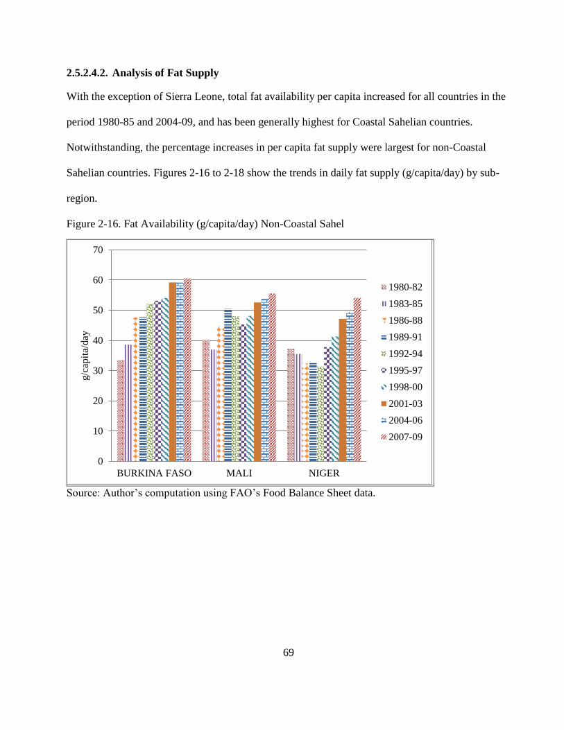
69
2.5.2.4.2. Analysis of Fat Supply
With the exception of Sierra Leone, total fat availability per capita increased for all countries in the
period 1980-85 and 2004-09, and has been generally highest for Coastal Sahelian countries.
Notwithstanding, the percentage increases in per capita fat supply were largest for non-Coastal
Sahelian countries. Figures 2-16 to 2-18 show the trends in daily fat supply (g/capita/day) by sub-
region.
Figure 2-16. Fat Availability (g/capita/day) Non-Coastal Sahel
Source: Author’s computation using FAO’s Food Balance Sheet data.
0
10
20
30
40
50
60
70
BURKINA FASO MALI NIGER
g/c
apit
a/day
1980-82
1983-85
1986-88
1989-91
1992-94
1995-97
1998-00
2001-03
2004-06
2007-09
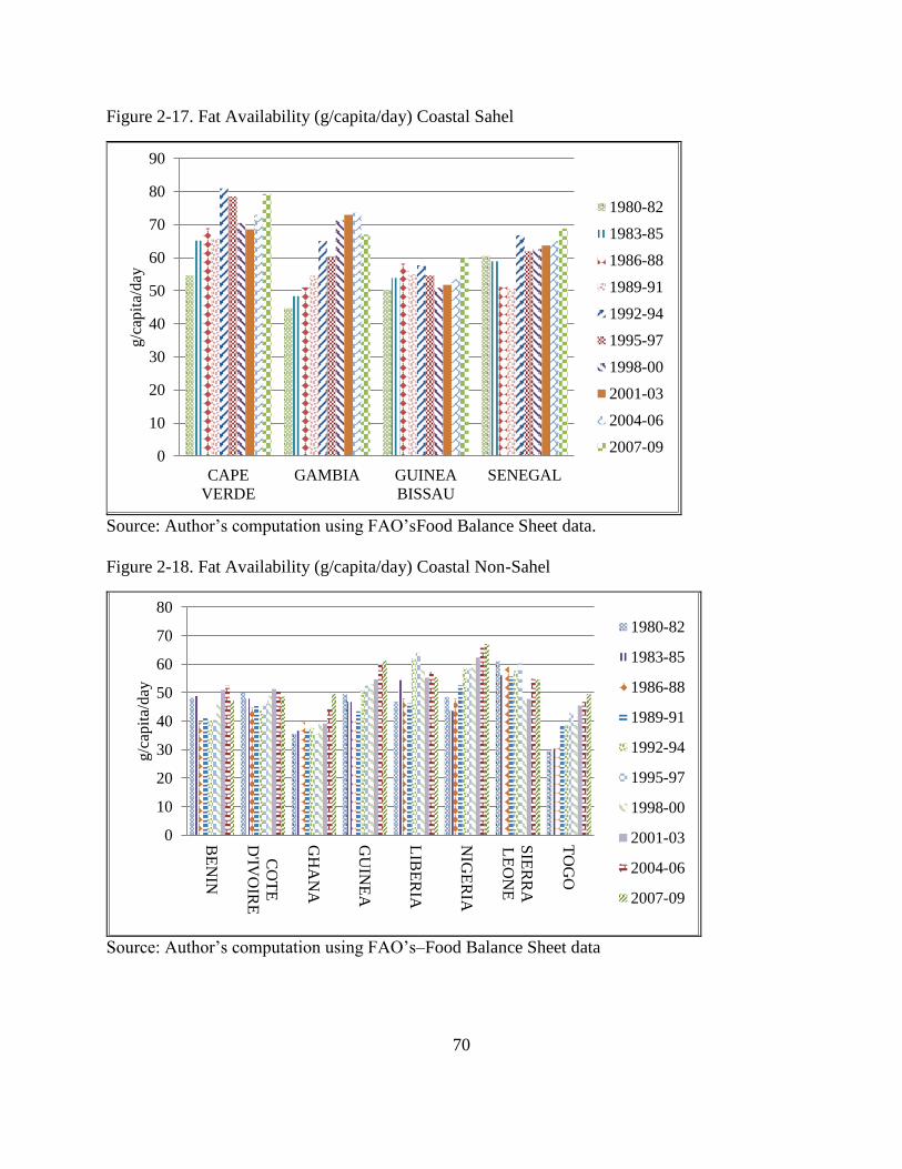
70
Figure 2-17. Fat Availability (g/capita/day) Coastal Sahel
Source: Author’s computation using FAO’sFood Balance Sheet data.
Figure 2-18. Fat Availability (g/capita/day) Coastal Non-Sahel
Source: Author’s computation using FAO’s–Food Balance Sheet data
0
10
20
30
40
50
60
70
80
90
CAPE
VERDE
GAMBIA GUINEA
BISSAU
SENEGAL
g/c
apit
a/d
ay
1980-82
1983-85
1986-88
1989-91
1992-94
1995-97
1998-00
2001-03
2004-06
2007-09
0
10
20
30
40
50
60
70
80
BE
NIN
CO
TE
D'IV
OIR
E
GH
AN
A
GU
INE
A
LIB
ER
IA
NIG
ER
IA
SIE
RR
A
LE
ON
E
TO
GO
g/c
apit
a/day
1980-82
1983-85
1986-88
1989-91
1992-94
1995-97
1998-00
2001-03
2004-06
2007-09
71
2.5.2.5. Trends in the Share of Macronutrient Group in Daily Per Capita Energy Supply
The contribution of various macronutrient groups to total daily per capita energy supply is one
indicator of diet quality. This section examines whether the composition of per capita food supply
in terms of major macronutrient groups is becoming more balanced, based on the joint FAO/WHO
guidelines for various nutrients for a balanced diet—55-75% of total calories from carbohydrates,
15-35% from fats and 10-15% from proteins (Nishida et al. 2004). The analysis reveals that over
time, while most countries in ECOWAS-WA have remained close to the upper bound of the daily
recommended share of carbohydrates in energy supply, few of these countries deviate from the
lower bound of the recommended share of protein and fats in daily energy supply.
2.5.2.5.1. Non-Coastal Sahel
Figure 2-19 shows the trends in the share of various macronutrient groups in total daily energy
supply per capita in the Non-Coastal Sahel. (See Me-Nsope and Staatz (2013) for the underlying
data for this and the other sub-regions.) The share of protein, fats, and carbohydrates in total daily
energy supply has not changed much. In particular, the share of protein seems almost constant over
time, as minor redistributions takes place between fats and carbohydrates. Nonetheless, since total
per capita calorie availability increased markedly for these countries over the study period, the
absolute levels of fat and protein consumption also increased substantially. In addition, we saw
from the analysis of protein by source in the Non-Coastal Sahel that the contribution of animal
protein has been growing since the early 2000s. Thus, in spite of the almost constant share of
protein in total daily energy supply, the quality of protein supply has improved to some extent due
to the growth in consumption of animal protein.
72
2.5.2.5.2. Coastal Sahel
In the Coastal Sahel (Figure 2-20), the share of carbohydrates still remains close to the upper bound
of the daily-recommended share. The share of protein has also remained close to its daily-
recommended lower bound (10-15%). The Gambia and Guinea Bissau over time have fallen below
the minimum daily protein share in total daily energy supply. As was the case in the Non-Coastal
Sahel, just focusing on the share of protein in total daily energy supply obscures the important
changes that have taken place (in particular in Cape Verde) in terms of the quality of protein supply.
The share of fat in daily energy supply has been much higher in the Coastal Sahel than in the Non-
Coastal Sahel.
2.5.2.5.3. Coastal Non-Sahel
In the Coastal Non-Sahel region, a similar pattern of not much variation in the share of each
macronutrient group in daily per capita energy supply is observed (Figure 2-21). However, unlike in
the case of the Coastal and Non-Coastal Sahel, the share of protein in daily energy, over time, and
for almost all Coastal Non-Sahelian countries, has remained below the recommended daily protein
share (10%) in total daily energy supply. With the exception of Sierra Leone, which has shown a
slight increase in protein share over time, protein share in all the other countries has been either
constant or declining. It is, however, worth noting that while the share of protein in total daily
energy supply has not shown much change, the analysis of protein supply in absolute terms as well
as of the contribution of animal protein to total protein supply seen earlier revealed not only an
increase in the amount of protein supplied over time (Benin, Ghana, Nigeria, Sierra Leone), but also
73
an increase in the quality of protein supply over time (Ghana, Nigeria21 and Sierra Leone). Ghana
and Cote d’Ivoire have consistently had higher than the daily-recommended carbohydrate share
over time, and this seems not to be changing much. This is not surprising because of the high
consumption of starchy roots and tubers in these countries. Guinea, Liberia, and Togo, in contrast,
have experienced a decline in the share of carbohydrates towards the upper bound of the
recommended daily share.
21 In Nigeria, the increase in the supply of protein from pulses per capita over time offsets the
decline in animal protein supply per capita, so that overall, the supply of high quality protein
(pulses and animal sources) increased over time.

74
Figure 2-19. Daily Caloric Share (%) by Macronutrients - Non-Coastal Sahel
Source: Author’s computation using FAO’s Food Balance Sheet data
0%
10%
20%
30%
40%
50%
60%
70%
80%
90%
100%
1980-8
2
1983-8
5
1986-8
8
1989-9
1
1992-9
4
1995-9
7
1998-0
0
2001-0
3
2004-0
6
2007-0
9
1980-8
2
1983-8
5
1986-8
8
1989-9
1
1992-9
4
1995-9
7
1998-0
0
2001-0
3
2004-0
6
2007-0
9
1980-8
2
1983-8
5
1986-8
8
1989-9
1
1992-9
4
1995-9
7
1998-0
0
2001-0
3
2004-0
6
2007-0
9
Burkina Faso Mali Niger
Protein Fat Carbohydrates
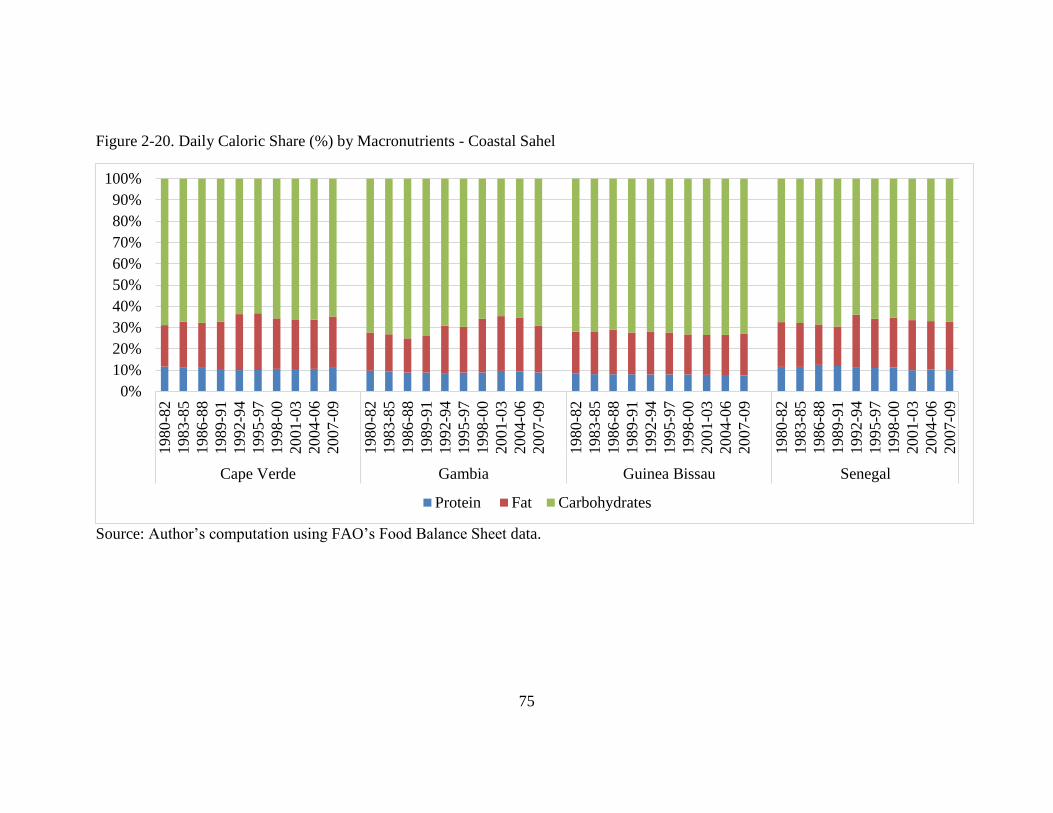
75
Figure 2-20. Daily Caloric Share (%) by Macronutrients - Coastal Sahel
Source: Author’s computation using FAO’s Food Balance Sheet data.
0%
10%
20%
30%
40%
50%
60%
70%
80%
90%
100%1980-8
2
1983-8
5
1986-8
8
1989-9
1
1992-9
4
1995-9
7
1998-0
0
2001-0
3
2004-0
6
2007-0
9
1980-8
2
1983-8
5
1986-8
8
1989-9
1
1992-9
4
1995-9
7
1998-0
0
2001-0
3
2004-0
6
2007-0
9
1980-8
2
1983-8
5
1986-8
8
1989-9
1
1992-9
4
1995-9
7
1998-0
0
2001-0
3
2004-0
6
2007-0
9
1980-8
2
1983-8
5
1986-8
8
1989-9
1
1992-9
4
1995-9
7
1998-0
0
2001-0
3
2004-0
6
2007-0
9
Cape Verde Gambia Guinea Bissau Senegal
Protein Fat Carbohydrates
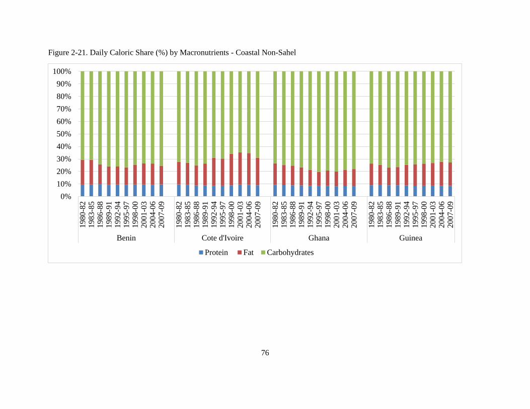
76
Figure 2-21. Daily Caloric Share (%) by Macronutrients - Coastal Non-Sahel
0%
10%
20%
30%
40%
50%
60%
70%
80%
90%
100%
1980-8
21983-8
51986-8
81989-9
11992-9
41995-9
71998-0
02001-0
32004-0
62007-0
9
1980-8
21983-8
51986-8
81989-9
11992-9
41995-9
71998-0
02001-0
32004-0
62007-0
9
1980-8
21983-8
51986-8
81989-9
11992-9
41995-9
71998-0
02001-0
32004-0
62007-0
9
1980-8
21983-8
51986-8
81989-9
11992-9
41995-9
71998-0
02001-0
32004-0
62007-0
9
Benin Cote d'Ivoire Ghana Guinea
Protein Fat Carbohydrates
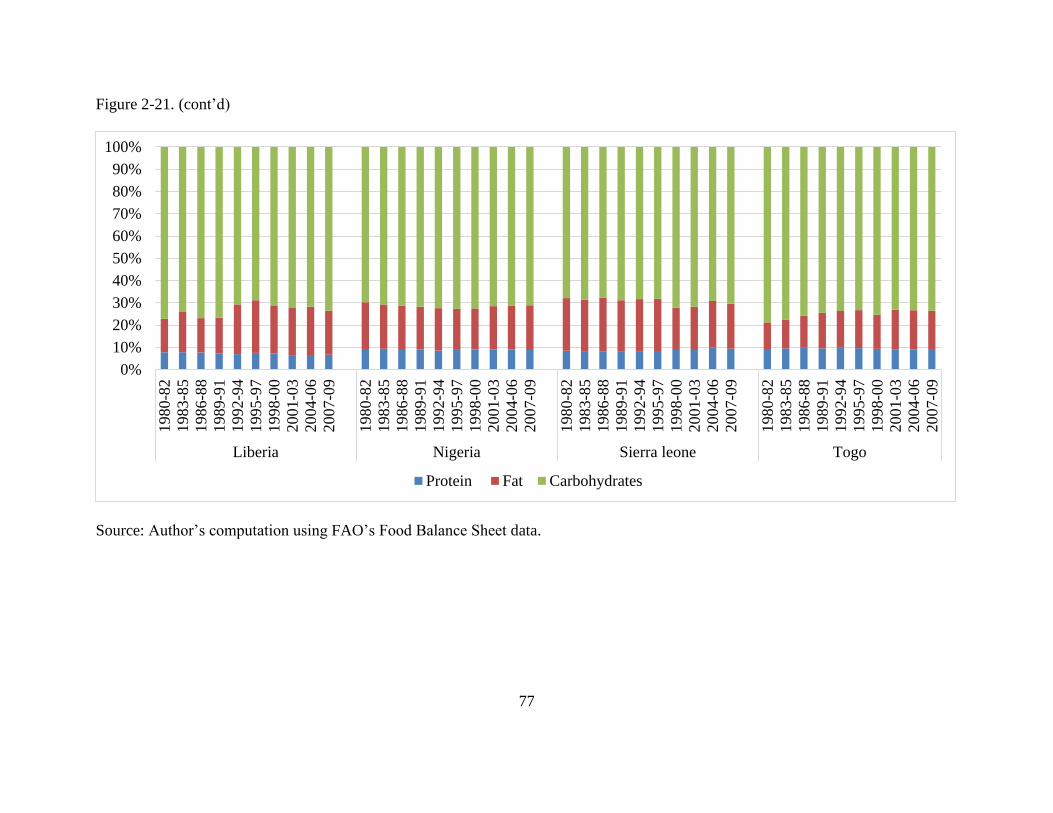
77
Figure 2-21. (cont’d)
Source: Author’s computation using FAO’s Food Balance Sheet data.
0%
10%
20%
30%
40%
50%
60%
70%
80%
90%
100%1980-8
2
1983-8
5
1986-8
8
1989-9
1
1992-9
4
1995-9
7
1998-0
0
2001-0
3
2004-0
6
2007-0
9
1980-8
2
1983-8
5
1986-8
8
1989-9
1
1992-9
4
1995-9
7
1998-0
0
2001-0
3
2004-0
6
2007-0
9
1980-8
2
1983-8
5
1986-8
8
1989-9
1
1992-9
4
1995-9
7
1998-0
0
2001-0
3
2004-0
6
2007-0
9
1980-8
2
1983-8
5
1986-8
8
1989-9
1
1992-9
4
1995-9
7
1998-0
0
2001-0
3
2004-0
6
2007-0
9
Liberia Nigeria Sierra leone Togo
Protein Fat Carbohydrates
78
2.6. Chapter Summary
The goal of this chapter was to provide evidence of shifts in per capita food availability patterns
in ECOWAS West Africa. In particular, the analysis was intended to identify major contributors
to diets, changes in the levels as well as in the composition of per capita food supply at the
country-level and to enhance understanding of the food supply situation within the ECOWAS
using national-level FAOSTAT’s food balance sheet data from 1980-2009. The analysis reveals
a trend towards greater calorie supply for most ECOWAS countries. The growth in daily energy
availability has been much more pronounced and consistent for countries experiencing rapid
economic growth (e.g., Ghana and Cape Verde), but has been disrupted in countries that have
been through civil disruptions like Cote d’Ivoire, Liberia and Sierra Leone.
The analysis also provides evidence of a diversification in the composition of food
supply. The relative importance of starchy roots and tubers in total food availability, particularly
in the Sahel region, has grown over time. The analysis reveals evidence consistent with the
“cassava revolution” that has taken place in some of the Coastal Non-Sahelian countries such as
Nigeria, Ghana, and Sierra Leone (Nweke et al., 2002). The growth in the per capita availability
of cassava (e.g., Senegal) and sweet potatoes (e.g., Mali) most likely reflects the lower income
population shifting towards cheaper calorie sources. Per capita availability of yams also showed
huge increases in some Coastal Non-Sahelian countries (e.g., Ghana and Nigeria). There has also
been positive growth in the supply of Irish potatoes in some countries (e.g., Cape Verde and
Senegal), supporting evidence of a westernization of diets (increased consumption of potato
chips/French fries). The analysis also provides evidence of a striking growth in per capita
availability of maize in the Sahel (Burkina Faso, Mali, and Senegal). Per capita rice availability
increased for most countries in the study period. In Cape Verde, for example, there is been a
79
replacement of maize with rice as the dominant type of cereal. Although food availability is only
one dimension of food security, rising starchy staple availability is likely to have a positive
impact for food security in the region.
With respect to the quality of the per capita food supply, the supply of daily protein
per capita has been increasing for most countries since the early 2000s. Proteins from plant
sources are the dominant source of protein in the entire region. Although plant protein dominates
as the major source of protein for most of these countries, some of these countries (e.g., Niger,
Sierra Leone, Nigeria and Cape Verde) derive an important share of vegetable protein from
pulses, which are also a source of high-quality protein. Some countries have shown a positive
trend in the supply of animal protein. The countries that have shown evidence of diet upgrading
through increased per capita availability of animal protein have been mostly those that have also
shown evidence of rapid and strong economic growth over time (e.g., Ghana and Cape Verde).
Countries with modest economic growth, such as Mali, have also shown modest growth in the
consumption of animal protein over time. Apparent per capita daily fat supply increased for most
countries in the study period. The share of carbohydrates, fats, and proteins in total daily energy
(calorie) supply, however, did not change much over time. While most countries meet and even
exceed the WHO/FAO recommended daily allowance (measured as shares) for carbohydrates,
the share of protein in daily energy continues to remain close to the lower bound of the
recommended daily value. However, this has not always meant that the diets have not improved
over time, as some countries have experienced not only a positive growth in the supply of
proteins in absolute terms, but also have been improving in terms of the availability of animal
protein as well as pulses. Although fish and seafood remain the main animal protein source for

80
most of the coastal states in the ECOWAS zone, most of the countries in the region have
experienced growth in the per capita supply of poultry meat over time, primarily from imports.

81
APPENDIX
82
Table A2-1. Food Availability by Major Food Group–Non-Coastal Sahel- Burkina Faso (kg/capita/year)
Food Group 1980
to
1982
1983
to
1985
1986
to
1988
1989
to
1991
1992
to
1994
1995
to
1997
1998
to
2000
2001
to
2003
2004
to
2006
2007
to
2009
% change
1980-85 to
2004-09
Cereals - Excl. Beer 148 148 196 217 229 224 218 224 232 228 55%
Starchy R & T 17 17 15 7 7 6 6 6 7 8 -56%
Sugar & Sweeteners 4 4 4 4 4 5 4 5 5 5 25%
Pulses 10 9 12 12 13 11 12 12 13 13 37%
Oilcrops 6 8 11 9 12 11 12 15 12 14 86%
Vegetable Oils 3 4 4 4 4 5 5 5 6 6 71%
Fruits Excl. wine 8 8 7 7 7 6 6 6 5 5 -38%
Vegetables- 21 23 22 24 23 21 19 17 17 15 -27%
Meat & offal 9 11 12 15 16 16 17 18 19 18 85%
Eggs 1 1 1 2 3 3 2 2 2 2 100%
Milk - Excl. Butter 26 22 23 16 16 17 18 16 17 17 -29%
Fish & Seafood 2 2 2 2 2 2 2 2 2 2 15%
Alcoholic Beverages 50 46 55 54 63 61 52 55 54 54 13%
Source: Author’s computation using FAO’s Food Balance Sheet data.
83
Table A2-2. Food Availability by Major Food Group - Mali (kg/capita/year)
Food Group 1980
to
1982
1983
to
1985
1986
to
1988
1989
to
1991
1992
to
1994
1995
to
1997
1998
to
2000
2001
to
2003
2004
to
2006
2007
to
2009
% change
1980-85 to
2004-09
Cereals 125 155 185 181 176 181 181 189 198 204 44%
Starchy R&T 4 3 3 5 8 9 13 18 26 32 729%
Sugar & Sweeteners 4 4 6 10 10 11 13 13 13 12 213%
Pulses 4 4 5 6 10 9 12 11 10 7 113%
Vegetable Oils 6 5 7 8 8 7 8 8 8 8 45%
Fruits - Excl. Wine 17 17 18 17 19 23 24 26 30 28 71%
Vegetables 46 49 51 54 51 53 52 52 47 52 4%
Meat & offal 20 19 20 21 18 18 19 21 23 25 23%
Eggs 1 1 1 1 1 1 1 1 0 0 -100%
Milk Excl. Butter 59 47 46 51 51 48 52 52 57 63 13%
Fish, Seafood 10 7 7 8 7 11 9 9 9 8 0%
Alcoholic Beverages 5 6 7 7 5 6 5 6 6 6 9%
Source: Author’s computation using FAO’s Food Balance Sheet data.
84
Table A2-3. Food Availability by Major Food Group–Non-Coastal Sahel - Niger (kg/capita/year)
Food Group 1980
to
1982
1983
to
1985
1986
to
1988
1989
to
1991
1992
to
1994
1995
to
1997
1998
to
2000
2001
to
2003
2004
to
2006
2007
to
2009
%change
1980-85 to
2004-09
Cereals Excl. Beer 197 201 199 211 200 200 200 202 200 209 3%
Starchy R & T 31 32 29 21 14 17 22 14 14 13 -57%
Sugar & Sweeteners 4 7 7 5 3 6 7 6 7 6 18%
Pulses 23 18 18 15 14 14 24 19 23 36 44%
Vegetable Oils 3 3 2 3 2 4 4 5 5 4 50%
Fruits - Excl. Wine 7 7 6 6 5 5 6 10 12 15 93%
Vegetables 21 16 16 30 34 41 49 54 49 51 170%
Meat and offal 27 22 19 20 21 21 23 25 27 28 12%
Eggs 1 1 1 1 1 1 0 0 0 0 -100%
Fish & Seafood 1 0 0 1 0 1 1 1 3 3 218%
Milk Excl. Butter 57 52 42 40 40 43 45 48 49 59 -1%
Alcoholic Beverages 2 1 1 1 0 1 1 0 0 1 -67%
Source: Author’s computation using FAO’s Food Balance Sheet data.
85
Table A2-4. Food Availability by Major Food Group - Coastal Non-Sahel- Benin (kg/capita)
Food Group 1980
to
1982
1983
to
1985
1986
to
1988
1989
to
1991
1992
to
1994
1995
to
1997
1998
to
2000
2001
to
2003
2004
to
2006
2007
to
2009
% change
1980-85 to
2004-09
Cereals – Excl. Beer 93 92 97 109 107 108 108 108 114 115 24%
Starchy R&T 205 212 229 268 266 283 287 289 278 296 38%
Sugar & Sweeteners 0 2 3 4 6 7 6 6 4 6 400%
pulses 6 7 8 9 9 9 10 10 12 17 123%
Oilcrops 7 7 7 8 8 9 9 10 9 8 21%
Vegetable Oils 9 9 6 6 5 5 7 8 9 7 -11%
Fruits Excl. wine 36 35 33 34 31 32 29 30 30 37 -6%
Vegetables- 37 38 42 43 46 49 54 49 48 48 28%
Meat & offal 13 16 13 11 13 12 14 17 14 20 17%
Eggs 2 2 2 1 1 1 1 1 1 1 -50%
Milk – Excl. Butter 8 8 8 6 6 8 12 11 10 8 13%
Fish & Seafood 12 10 11 9 10 10 8 9 9 8 -23%
Alcoholic Beverages 14 12 12 12 11 12 11 12 14 15 12%
Source: Author’s computation using FAO’s Food Balance Sheet data.
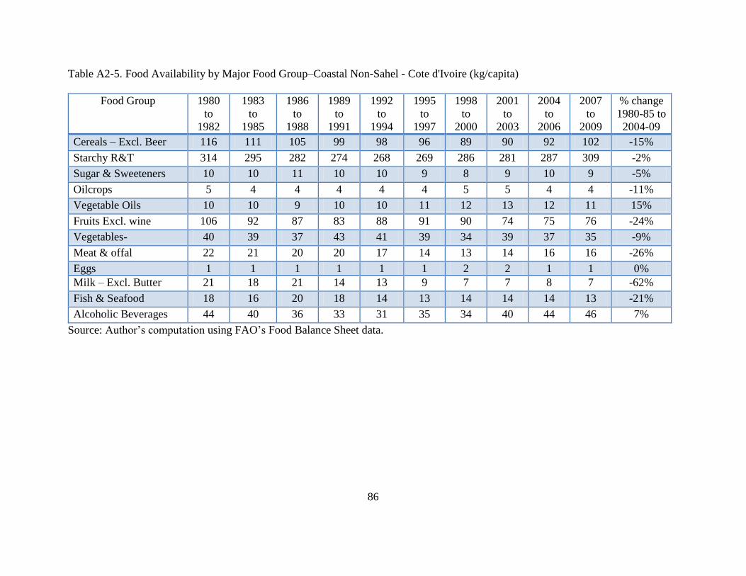
86
Table A2-5. Food Availability by Major Food Group–Coastal Non-Sahel - Cote d'Ivoire (kg/capita)
Food Group 1980
to
1982
1983
to
1985
1986
to
1988
1989
to
1991
1992
to
1994
1995
to
1997
1998
to
2000
2001
to
2003
2004
to
2006
2007
to
2009
% change
1980-85 to
2004-09
Cereals – Excl. Beer 116 111 105 99 98 96 89 90 92 102 -15%
Starchy R&T 314 295 282 274 268 269 286 281 287 309 -2%
Sugar & Sweeteners 10 10 11 10 10 9 8 9 10 9 -5%
Oilcrops 5 4 4 4 4 4 5 5 4 4 -11%
Vegetable Oils 10 10 9 10 10 11 12 13 12 11 15%
Fruits Excl. wine 106 92 87 83 88 91 90 74 75 76 -24%
Vegetables- 40 39 37 43 41 39 34 39 37 35 -9%
Meat & offal 22 21 20 20 17 14 13 14 16 16 -26%
Eggs 1 1 1 1 1 1 2 2 1 1 0%
Milk – Excl. Butter 21 18 21 14 13 9 7 7 8 7 -62%
Fish & Seafood 18 16 20 18 14 13 14 14 14 13 -21%
Alcoholic Beverages 44 40 36 33 31 35 34 40 44 46 7%
Source: Author’s computation using FAO’s Food Balance Sheet data.
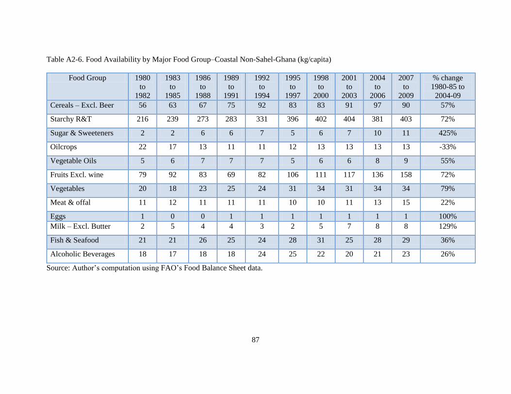
87
Table A2-6. Food Availability by Major Food Group–Coastal Non-Sahel-Ghana (kg/capita)
Food Group 1980
to
1982
1983
to
1985
1986
to
1988
1989
to
1991
1992
to
1994
1995
to
1997
1998
to
2000
2001
to
2003
2004
to
2006
2007
to
2009
% change
1980-85 to
2004-09
Cereals – Excl. Beer 56 63 67 75 92 83 83 91 97 90 57%
Starchy R&T 216 239 273 283 331 396 402 404 381 403 72%
Sugar & Sweeteners 2 2 6 6 7 5 6 7 10 11 425%
Oilcrops 22 17 13 11 11 12 13 13 13 13 -33%
Vegetable Oils 5 6 7 7 7 5 6 6 8 9 55%
Fruits Excl. wine 79 92 83 69 82 106 111 117 136 158 72%
Vegetables 20 18 23 25 24 31 34 31 34 34 79%
Meat & offal 11 12 11 11 11 10 10 11 13 15 22%
Eggs 1 0 0 1 1 1 1 1 1 1 100%
Milk – Excl. Butter 2 5 4 4 3 2 5 7 8 8 129%
Fish & Seafood 21 21 26 25 24 28 31 25 28 29 36%
Alcoholic Beverages 18 17 18 18 24 25 22 20 21 23 26%
Source: Author’s computation using FAO’s Food Balance Sheet data.
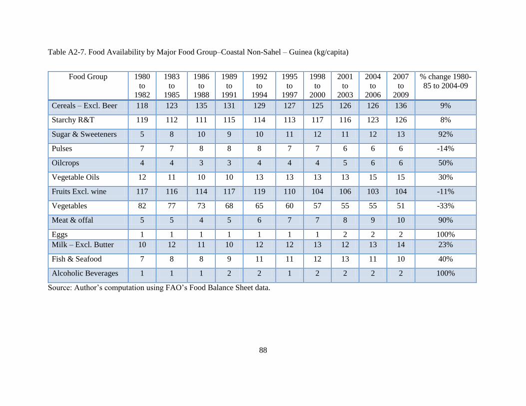
88
Table A2-7. Food Availability by Major Food Group–Coastal Non-Sahel – Guinea (kg/capita)
Source: Author’s computation using FAO’s Food Balance Sheet data.
Food Group 1980
to
1982
1983
to
1985
1986
to
1988
1989
to
1991
1992
to
1994
1995
to
1997
1998
to
2000
2001
to
2003
2004
to
2006
2007
to
2009
% change 1980-
85 to 2004-09
Cereals – Excl. Beer 118 123 135 131 129 127 125 126 126 136 9%
Starchy R&T 119 112 111 115 114 113 117 116 123 126 8%
Sugar & Sweeteners 5 8 10 9 10 11 12 11 12 13 92%
Pulses 7 7 8 8 8 7 7 6 6 6 -14%
Oilcrops 4 4 3 3 4 4 4 5 6 6 50%
Vegetable Oils 12 11 10 10 13 13 13 13 15 15 30%
Fruits Excl. wine 117 116 114 117 119 110 104 106 103 104 -11%
Vegetables 82 77 73 68 65 60 57 55 55 51 -33%
Meat & offal 5 5 4 5 6 7 7 8 9 10 90%
Eggs 1 1 1 1 1 1 1 2 2 2 100%
Milk – Excl. Butter 10 12 11 10 12 12 13 12 13 14 23%
Fish & Seafood 7 8 8 9 11 11 12 13 11 10 40%
Alcoholic Beverages 1 1 1 2 2 1 2 2 2 2 100%
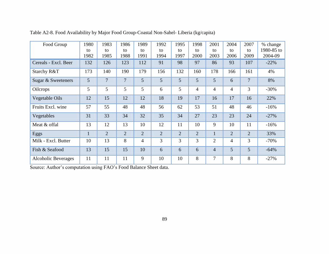
89
Table A2-8. Food Availability by Major Food Group-Coastal Non-Sahel- Liberia (kg/capita)
Food Group 1980
to
1982
1983
to
1985
1986
to
1988
1989
to
1991
1992
to
1994
1995
to
1997
1998
to
2000
2001
to
2003
2004
to
2006
2007
to
2009
% change
1980-85 to
2004-09
Cereals - Excl. Beer 132 126 123 112 91 98 97 86 93 107 -22%
Starchy R&T 173 140 190 179 156 132 160 178 166 161 4%
Sugar & Sweeteners 5 7 7 5 5 5 5 5 6 7 8%
Oilcrops 5 5 5 5 6 5 4 4 4 3 -30%
Vegetable Oils 12 15 12 12 18 19 17 16 17 16 22%
Fruits Excl. wine 57 55 48 48 56 62 53 51 48 46 -16%
Vegetables 31 33 34 32 35 34 27 23 23 24 -27%
Meat & offal 13 12 13 10 12 11 10 9 10 11 -16%
Eggs 1 2 2 2 2 2 2 1 2 2 33%
Milk - Excl. Butter 10 13 8 4 3 3 3 2 4 3 -70%
Fish & Seafood 13 15 15 10 6 6 6 4 5 5 -64%
Alcoholic Beverages 11 11 11 9 10 10 8 7 8 8 -27%
Source: Author’s computation using FAO’s Food Balance Sheet data.
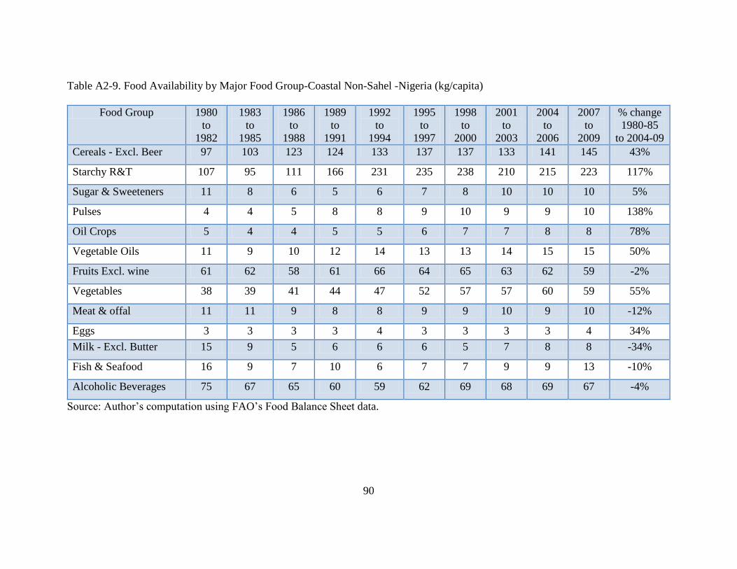
90
Table A2-9. Food Availability by Major Food Group-Coastal Non-Sahel -Nigeria (kg/capita)
Food Group 1980
to
1982
1983
to
1985
1986
to
1988
1989
to
1991
1992
to
1994
1995
to
1997
1998
to
2000
2001
to
2003
2004
to
2006
2007
to
2009
% change
1980-85
to 2004-09
Cereals - Excl. Beer 97 103 123 124 133 137 137 133 141 145 43%
Starchy R&T 107 95 111 166 231 235 238 210 215 223 117%
Sugar & Sweeteners 11 8 6 5 6 7 8 10 10 10 5%
Pulses 4 4 5 8 8 9 10 9 9 10 138%
Oil Crops 5 4 4 5 5 6 7 7 8 8 78%
Vegetable Oils 11 9 10 12 14 13 13 14 15 15 50%
Fruits Excl. wine 61 62 58 61 66 64 65 63 62 59 -2%
Vegetables 38 39 41 44 47 52 57 57 60 59 55%
Meat & offal 11 11 9 8 8 9 9 10 9 10 -12%
Eggs 3 3 3 3 4 3 3 3 3 4 34%
Milk - Excl. Butter 15 9 5 6 6 6 5 7 8 8 -34%
Fish & Seafood 16 9 7 10 6 7 7 9 9 13 -10%
Alcoholic Beverages 75 67 65 60 59 62 69 68 69 67 -4%
Source: Author’s computation using FAO’s Food Balance Sheet data.
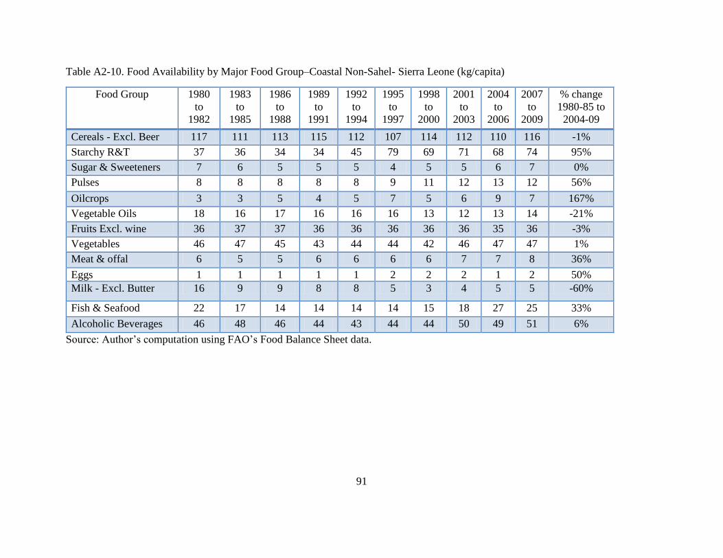
91
Table A2-10. Food Availability by Major Food Group–Coastal Non-Sahel- Sierra Leone (kg/capita)
Food Group 1980
to
1982
1983
to
1985
1986
to
1988
1989
to
1991
1992
to
1994
1995
to
1997
1998
to
2000
2001
to
2003
2004
to
2006
2007
to
2009
% change
1980-85 to
2004-09
Cereals - Excl. Beer 117 111 113 115 112 107 114 112 110 116 -1%
Starchy R&T 37 36 34 34 45 79 69 71 68 74 95%
Sugar & Sweeteners 7 6 5 5 5 4 5 5 6 7 0%
Pulses 8 8 8 8 8 9 11 12 13 12 56%
Oilcrops 3 3 5 4 5 7 5 6 9 7 167%
Vegetable Oils 18 16 17 16 16 16 13 12 13 14 -21%
Fruits Excl. wine 36 37 37 36 36 36 36 36 35 36 -3%
Vegetables 46 47 45 43 44 44 42 46 47 47 1%
Meat & offal 6 5 5 6 6 6 6 7 7 8 36%
Eggs 1 1 1 1 1 2 2 2 1 2 50%
Milk - Excl. Butter 16 9 9 8 8 5 3 4 5 5 -60%
Fish & Seafood 22 17 14 14 14 14 15 18 27 25 33%
Alcoholic Beverages 46 48 46 44 43 44 44 50 49 51 6%
Source: Author’s computation using FAO’s Food Balance Sheet data.
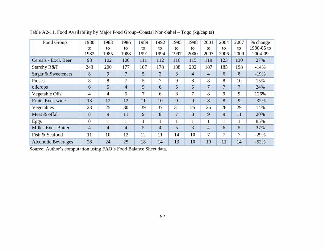
92
Table A2-11. Food Availability by Major Food Group–Coastal Non-Sahel – Togo (kg/capita)
Food Group 1980
to
1982
1983
to
1985
1986
to
1988
1989
to
1991
1992
to
1994
1995
to
1997
1998
to
2000
2001
to
2003
2004
to
2006
2007
to
2009
% change
1980-85 to
2004-09
Cereals - Excl. Beer 98 102 100 111 112 116 115 119 123 130 27%
Starchy R&T 243 200 177 187 178 188 202 187 185 198 -14%
Sugar & Sweeteners 8 9 7 5 2 3 4 4 6 8 -19%
Pulses 8 8 7 5 7 9 8 8 8 10 15%
oilcrops 6 5 4 5 6 5 5 7 7 7 24%
Vegetable Oils 4 4 5 7 6 8 7 8 9 9 126%
Fruits Excl. wine 13 12 12 11 10 9 9 8 8 9 -32%
Vegetables 23 25 30 39 37 31 25 25 26 29 14%
Meat & offal 8 9 11 9 8 7 8 9 9 11 20%
Eggs 0 1 1 1 1 1 1 1 1 1 85%
Milk - Excl. Butter 4 4 4 5 4 5 3 4 6 5 37%
Fish & Seafood 11 10 12 12 11 14 10 7 7 7 -29%
Alcoholic Beverages 28 24 25 18 14 13 10 10 11 14 -52%
Source: Author’s computation using FAO’s Food Balance Sheet data.
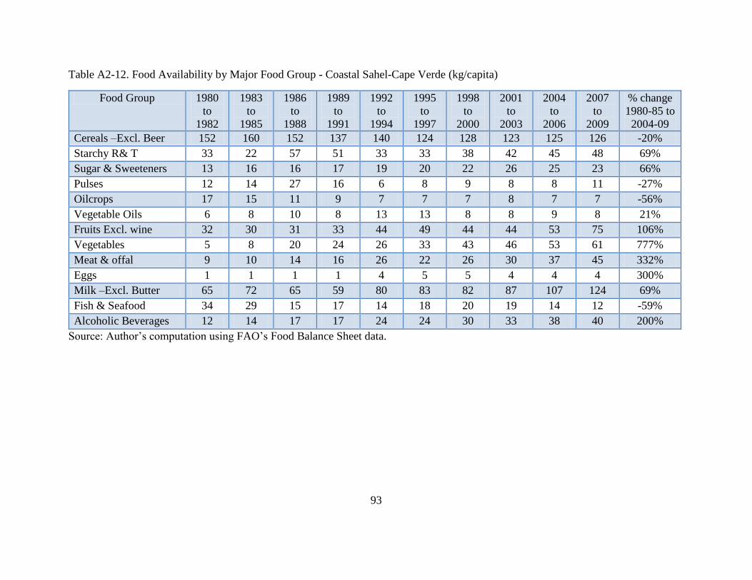
93
Table A2-12. Food Availability by Major Food Group - Coastal Sahel-Cape Verde (kg/capita)
Food Group 1980
to
1982
1983
to
1985
1986
to
1988
1989
to
1991
1992
to
1994
1995
to
1997
1998
to
2000
2001
to
2003
2004
to
2006
2007
to
2009
% change
1980-85 to
2004-09
Cereals –Excl. Beer 152 160 152 137 140 124 128 123 125 126 -20%
Starchy R& T 33 22 57 51 33 33 38 42 45 48 69%
Sugar & Sweeteners 13 16 16 17 19 20 22 26 25 23 66%
Pulses 12 14 27 16 6 8 9 8 8 11 -27%
Oilcrops 17 15 11 9 7 7 7 8 7 7 -56%
Vegetable Oils 6 8 10 8 13 13 8 8 9 8 21%
Fruits Excl. wine 32 30 31 33 44 49 44 44 53 75 106%
Vegetables 5 8 20 24 26 33 43 46 53 61 777%
Meat & offal 9 10 14 16 26 22 26 30 37 45 332%
Eggs 1 1 1 1 4 5 5 4 4 4 300%
Milk –Excl. Butter 65 72 65 59 80 83 82 87 107 124 69%
Fish & Seafood 34 29 15 17 14 18 20 19 14 12 -59%
Alcoholic Beverages 12 14 17 17 24 24 30 33 38 40 200%
Source: Author’s computation using FAO’s Food Balance Sheet data.
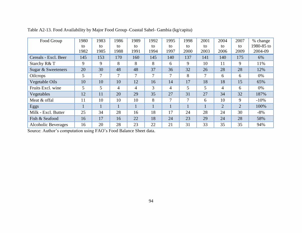
94
Table A2-13. Food Availability by Major Food Group–Coastal Sahel- Gambia (kg/capita)
Food Group 1980
to
1982
1983
to
1985
1986
to
1988
1989
to
1991
1992
to
1994
1995
to
1997
1998
to
2000
2001
to
2003
2004
to
2006
2007
to
2009
% change
1980-85 to
2004-09
Cereals - Excl. Beer 145 153 170 160 145 140 137 141 140 175 6%
Starchy R& T 9 9 8 8 8 6 9 10 11 9 11%
Sugar & Sweeteners 20 30 48 48 37 36 32 26 28 28 12%
Oilcrops 5 7 7 7 7 7 8 7 6 6 0%
Vegetable Oils 10 10 10 12 16 14 17 18 18 15 65%
Fruits Excl. wine 5 5 4 4 3 4 5 5 4 6 0%
Vegetables 12 11 20 29 35 27 31 27 34 32 187%
Meat & offal 11 10 10 10 8 7 7 6 10 9 -10%
Eggs 1 1 1 1 1 1 1 1 2 2 100%
Milk - Excl. Butter 25 34 28 16 18 17 24 28 24 30 -8%
Fish & Seafood 16 17 16 22 18 24 23 29 24 28 58%
Alcoholic Beverages 16 20 28 23 22 21 31 33 35 35 94%
Source: Author’s computation using FAO’s Food Balance Sheet data.
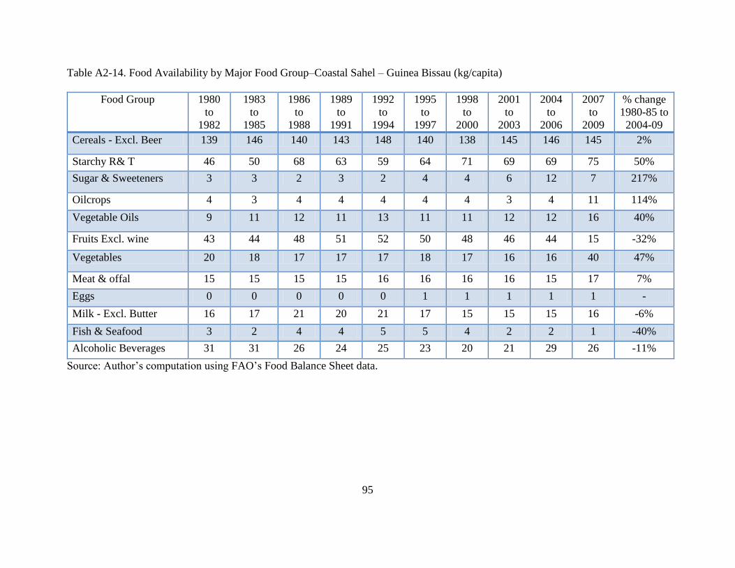
95
Table A2-14. Food Availability by Major Food Group–Coastal Sahel – Guinea Bissau (kg/capita)
Food Group 1980
to
1982
1983
to
1985
1986
to
1988
1989
to
1991
1992
to
1994
1995
to
1997
1998
to
2000
2001
to
2003
2004
to
2006
2007
to
2009
% change
1980-85 to
2004-09
Cereals - Excl. Beer 139 146 140 143 148 140 138 145 146 145 2%
Starchy R& T 46 50 68 63 59 64 71 69 69 75 50%
Sugar & Sweeteners 3 3 2 3 2 4 4 6 12 7 217%
Oilcrops 4 3 4 4 4 4 4 3 4 11 114%
Vegetable Oils 9 11 12 11 13 11 11 12 12 16 40%
Fruits Excl. wine 43 44 48 51 52 50 48 46 44 15 -32%
Vegetables 20 18 17 17 17 18 17 16 16 40 47%
Meat & offal 15 15 15 15 16 16 16 16 15 17 7%
Eggs 0 0 0 0 0 1 1 1 1 1 -
Milk - Excl. Butter 16 17 21 20 21 17 15 15 15 16 -6%
Fish & Seafood 3 2 4 4 5 5 4 2 2 1 -40%
Alcoholic Beverages 31 31 26 24 25 23 20 21 29 26 -11%
Source: Author’s computation using FAO’s Food Balance Sheet data.
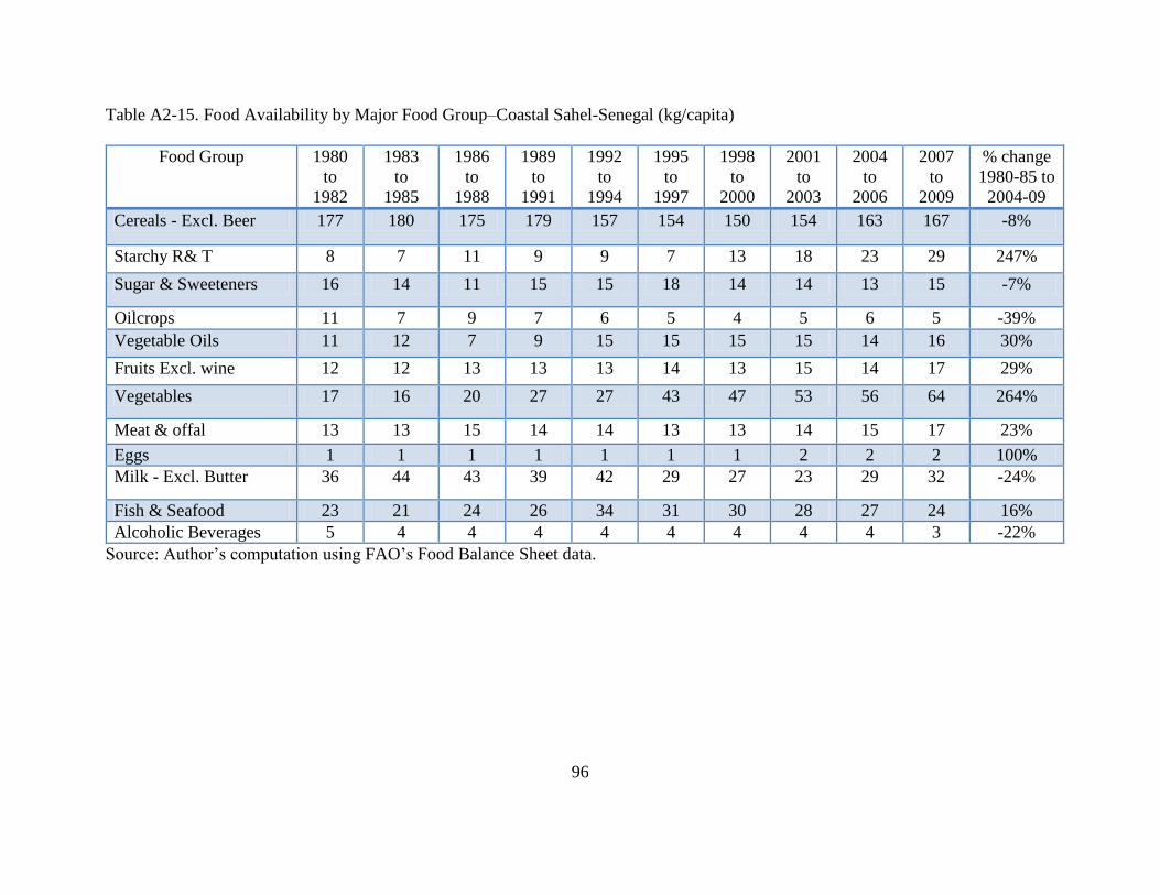
96
Table A2-15. Food Availability by Major Food Group–Coastal Sahel-Senegal (kg/capita)
Food Group 1980
to
1982
1983
to
1985
1986
to
1988
1989
to
1991
1992
to
1994
1995
to
1997
1998
to
2000
2001
to
2003
2004
to
2006
2007
to
2009
% change
1980-85 to
2004-09
Cereals - Excl. Beer 177 180 175 179 157 154 150 154 163 167 -8%
Starchy R& T 8 7 11 9 9 7 13 18 23 29 247%
Sugar & Sweeteners 16 14 11 15 15 18 14 14 13 15 -7%
Oilcrops 11 7 9 7 6 5 4 5 6 5 -39%
Vegetable Oils 11 12 7 9 15 15 15 15 14 16 30%
Fruits Excl. wine 12 12 13 13 13 14 13 15 14 17 29%
Vegetables 17 16 20 27 27 43 47 53 56 64 264%
Meat & offal 13 13 15 14 14 13 13 14 15 17 23%
Eggs 1 1 1 1 1 1 1 2 2 2 100%
Milk - Excl. Butter 36 44 43 39 42 29 27 23 29 32 -24%
Fish & Seafood 23 21 24 26 34 31 30 28 27 24 16%
Alcoholic Beverages 5 4 4 4 4 4 4 4 4 3 -22%
Source: Author’s computation using FAO’s Food Balance Sheet data.
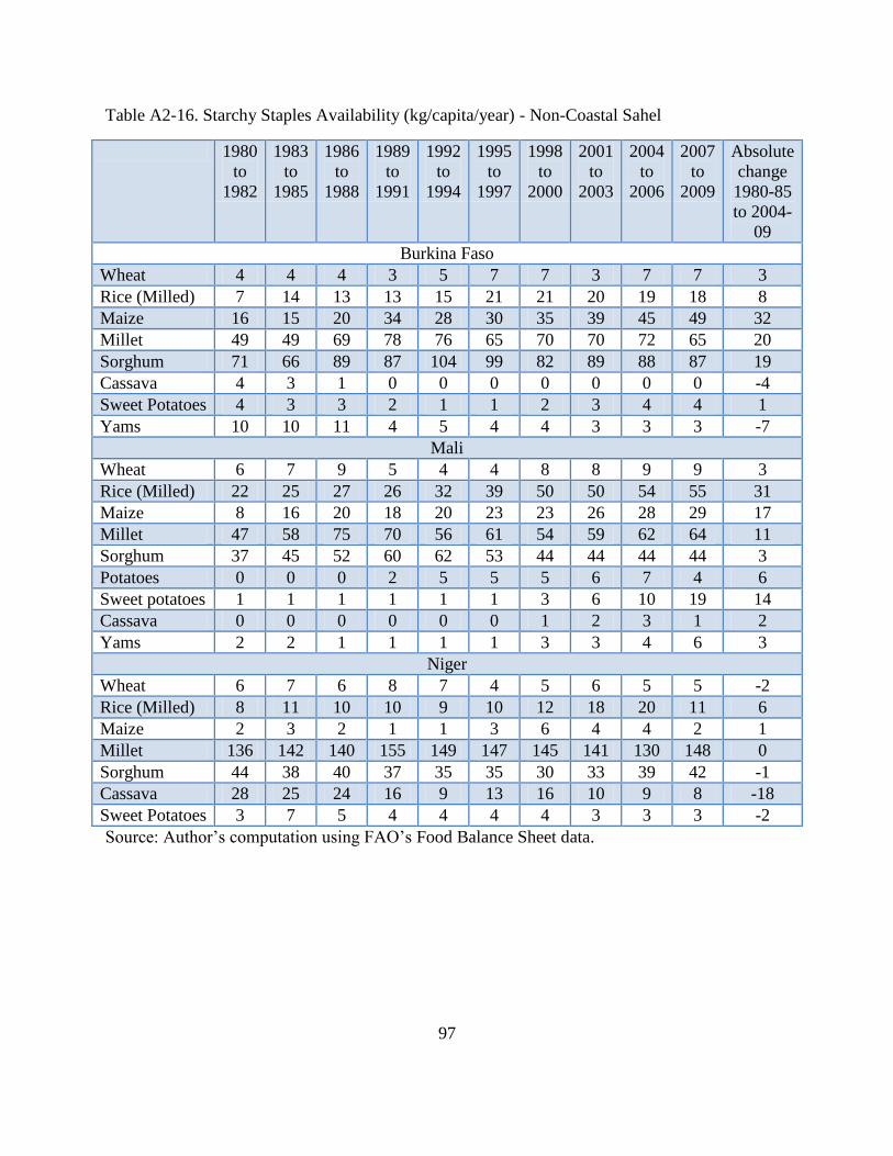
97
Table A2-16. Starchy Staples Availability (kg/capita/year) - Non-Coastal Sahel
1980
to
1982
1983
to
1985
1986
to
1988
1989
to
1991
1992
to
1994
1995
to
1997
1998
to
2000
2001
to
2003
2004
to
2006
2007
to
2009
Absolute
change
1980-85
to 2004-
09
Burkina Faso
Wheat 4 4 4 3 5 7 7 3 7 7 3
Rice (Milled) 7 14 13 13 15 21 21 20 19 18 8
Maize 16 15 20 34 28 30 35 39 45 49 32
Millet 49 49 69 78 76 65 70 70 72 65 20
Sorghum 71 66 89 87 104 99 82 89 88 87 19
Cassava 4 3 1 0 0 0 0 0 0 0 -4
Sweet Potatoes 4 3 3 2 1 1 2 3 4 4 1
Yams 10 10 11 4 5 4 4 3 3 3 -7
Mali
Wheat 6 7 9 5 4 4 8 8 9 9 3
Rice (Milled) 22 25 27 26 32 39 50 50 54 55 31
Maize 8 16 20 18 20 23 23 26 28 29 17
Millet 47 58 75 70 56 61 54 59 62 64 11
Sorghum 37 45 52 60 62 53 44 44 44 44 3
Potatoes 0 0 0 2 5 5 5 6 7 4 6
Sweet potatoes 1 1 1 1 1 1 3 6 10 19 14
Cassava 0 0 0 0 0 0 1 2 3 1 2
Yams 2 2 1 1 1 1 3 3 4 6 3
Niger
Wheat 6 7 6 8 7 4 5 6 5 5 -2
Rice (Milled) 8 11 10 10 9 10 12 18 20 11 6
Maize 2 3 2 1 1 3 6 4 4 2 1
Millet 136 142 140 155 149 147 145 141 130 148 0
Sorghum 44 38 40 37 35 35 30 33 39 42 -1
Cassava 28 25 24 16 9 13 16 10 9 8 -18
Sweet Potatoes 3 7 5 4 4 4 4 3 3 3 -2
Source: Author’s computation using FAO’s Food Balance Sheet data.
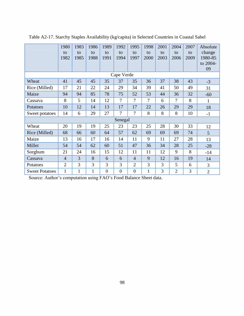
98
Table A2-17. Starchy Staples Availability (kg/capita) in Selected Countries in Coastal Sahel
1980
to
1982
1983
to
1985
1986
to
1988
1989
to
1991
1992
to
1994
1995
to
1997
1998
to
2000
2001
to
2003
2004
to
2006
2007
to
2009
Absolute
change
1980-85
to 2004-
09
Cape Verde
Wheat 41 45 45 35 37 35 36 37 38 43 -3
Rice (Milled) 17 21 22 24 29 34 39 41 50 49 31
Maize 94 94 85 78 75 52 53 44 36 32 -60
Cassava 8 5 14 12 7 7 7 6 7 8 1
Potatoes 10 12 14 13 17 17 22 26 29 29 18
Sweet potatoes 14 6 29 27 7 7 8 8 8 10 -1
Senegal
Wheat 20 19 19 25 23 23 25 28 30 33 12
Rice (Milled) 68 66 60 64 57 62 69 69 69 74 5
Maize 13 16 17 16 14 11 9 11 27 28 13
Millet 54 54 62 60 51 47 36 34 28 25 -28
Sorghum 21 24 16 15 12 11 11 12 9 8 -14
Cassava 4 3 8 6 6 4 9 12 16 19 14
Potatoes 2 3 3 3 3 2 3 3 5 6 3
Sweet Potatoes 1 1 1 0 0 0 1 3 2 3 2
Source: Author’s computation using FAO’s Food Balance Sheet data.
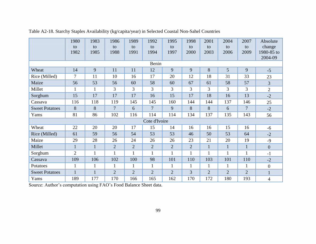
99
Table A2-18. Starchy Staples Availability (kg/capita/year) in Selected Coastal Non-Sahel Countries
1980
to
1982
1983
to
1985
1986
to
1988
1989
to
1991
1992
to
1994
1995
to
1997
1998
to
2000
2001
to
2003
2004
to
2006
2007
to
2009
Absolute
change
1980-85 to
2004-09
Benin
Wheat 14 9 11 11 12 9 9 8 5 9 -5
Rice (Milled) 7 11 10 16 17 20 12 18 31 33 23
Maize 56 53 56 60 58 60 67 61 58 57 3
Millet 1 1 3 3 3 3 3 3 3 3 2
Sorghum 15 17 17 17 16 15 17 18 16 13 -2
Cassava 116 118 119 145 145 160 144 144 137 146 25
Sweet Potatoes 8 8 7 6 7 9 8 8 6 7 -2
Yams 81 86 102 116 114 114 134 137 135 143 56
Cote d'Ivoire
Wheat 22 20 20 17 15 14 16 16 15 16 -6
Rice (Milled) 61 59 56 54 53 53 46 50 53 64 -2
Maize 29 28 26 24 26 26 23 21 20 19 -9
Millet 1 1 2 2 2 2 2 1 1 1 0
Sorghum 2 1 1 1 1 1 1 1 1 1 -1
Cassava 109 106 102 100 98 101 110 103 101 110 -2
Potatoes 1 1 1 1 1 1 1 1 1 1 0
Sweet Potatoes 1 1 2 2 2 2 3 2 2 2 1
Yams 189 177 170 166 165 162 170 172 180 193 4
Source: Author’s computation using FAO’s Food Balance Sheet data.
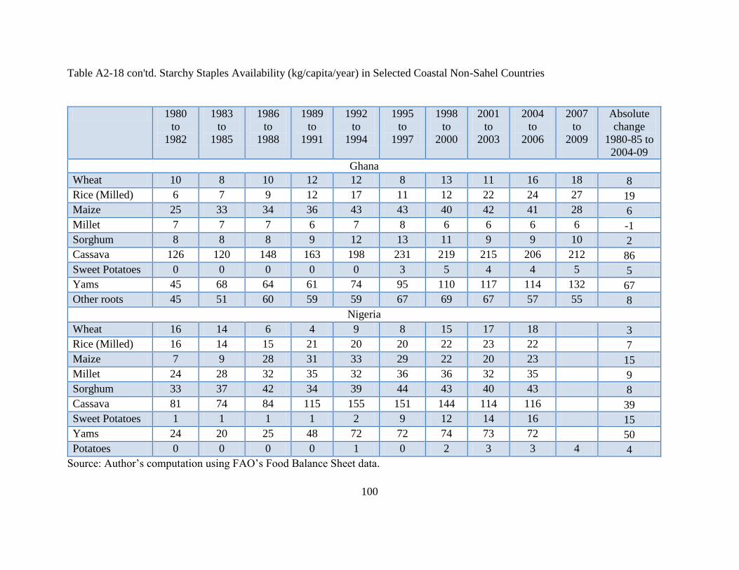
100
Table A2-18 con'td. Starchy Staples Availability (kg/capita/year) in Selected Coastal Non-Sahel Countries
Source: Author’s computation using FAO’s Food Balance Sheet data.
1980
to
1982
1983
to
1985
1986
to
1988
1989
to
1991
1992
to
1994
1995
to
1997
1998
to
2000
2001
to
2003
2004
to
2006
2007
to
2009
Absolute
change
1980-85 to
2004-09
Ghana
Wheat 10 8 10 12 12 8 13 11 16 18 8
Rice (Milled) 6 7 9 12 17 11 12 22 24 27 19
Maize 25 33 34 36 43 43 40 42 41 28 6
Millet 7 7 7 6 7 8 6 6 6 6 -1
Sorghum 8 8 8 9 12 13 11 9 9 10 2
Cassava 126 120 148 163 198 231 219 215 206 212 86
Sweet Potatoes 0 0 0 0 0 3 5 4 4 5 5
Yams 45 68 64 61 74 95 110 117 114 132 67
Other roots 45 51 60 59 59 67 69 67 57 55 8
Nigeria
Wheat 16 14 6 4 9 8 15 17 18 3
Rice (Milled) 16 14 15 21 20 20 22 23 22 7
Maize 7 9 28 31 33 29 22 20 23 15
Millet 24 28 32 35 32 36 36 32 35 9
Sorghum 33 37 42 34 39 44 43 40 43 8
Cassava 81 74 84 115 155 151 144 114 116 39
Sweet Potatoes 1 1 1 1 2 9 12 14 16 15
Yams 24 20 25 48 72 72 74 73 72 50
Potatoes 0 0 0 0 1 0 2 3 3 4 4
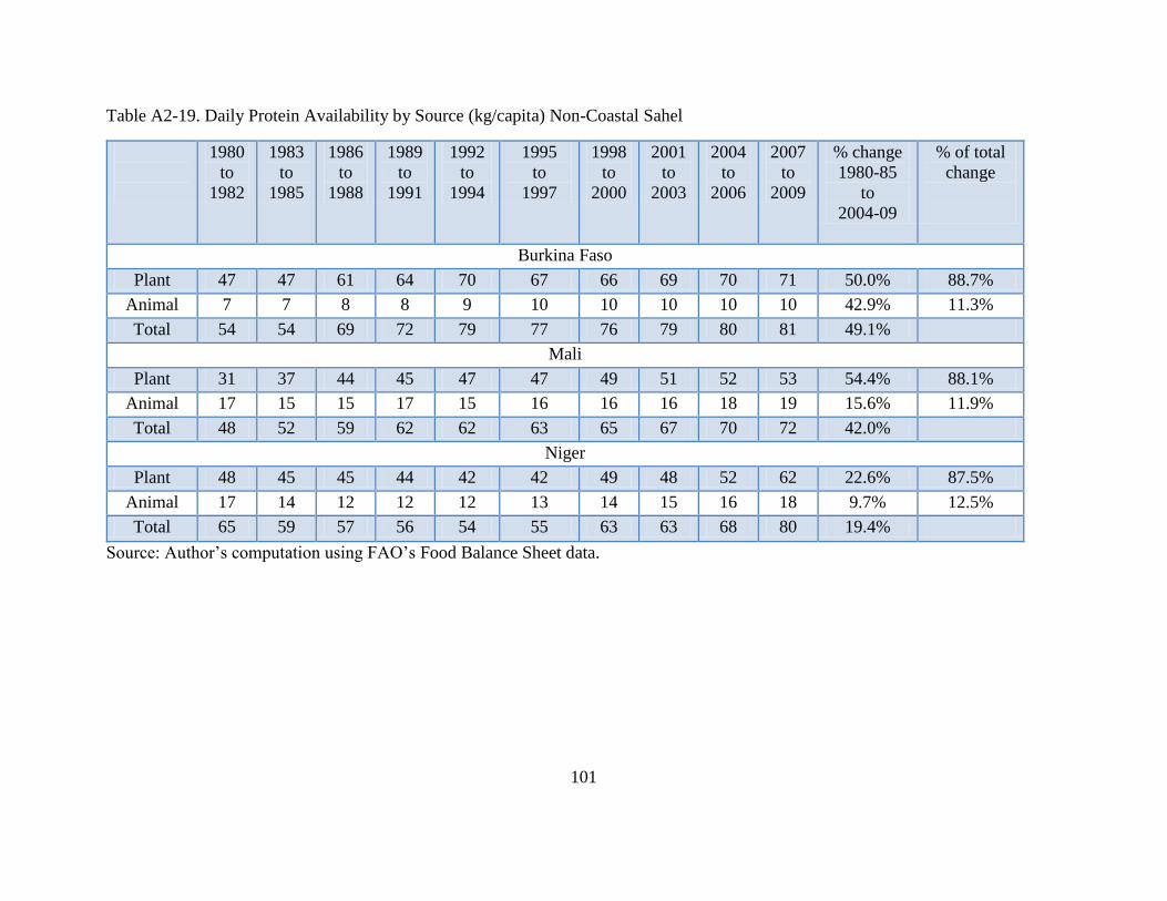
101
Table A2-19. Daily Protein Availability by Source (kg/capita) Non-Coastal Sahel
1980
to
1982
1983
to
1985
1986
to
1988
1989
to
1991
1992
to
1994
1995
to
1997
1998
to
2000
2001
to
2003
2004
to
2006
2007
to
2009
% change
1980-85
to
2004-09
% of total
change
Burkina Faso
Plant 47 47 61 64 70 67 66 69 70 71 50.0% 88.7%
Animal 7 7 8 8 9 10 10 10 10 10 42.9% 11.3%
Total 54 54 69 72 79 77 76 79 80 81 49.1%
Mali
Plant 31 37 44 45 47 47 49 51 52 53 54.4% 88.1%
Animal 17 15 15 17 15 16 16 16 18 19 15.6% 11.9%
Total 48 52 59 62 62 63 65 67 70 72 42.0%
Niger
Plant 48 45 45 44 42 42 49 48 52 62 22.6% 87.5%
Animal 17 14 12 12 12 13 14 15 16 18 9.7% 12.5%
Total 65 59 57 56 54 55 63 63 68 80 19.4%
Source: Author’s computation using FAO’s Food Balance Sheet data.
102
Table A2-20. Daily Protein Availability by Source (g/capita) Coastal Sahel
1980
to
1982
1983
to
1985
1986
to
1988
1989
to
1991
1992
to
1994
1995
to
1997
1998
to
2000
2001
to
2003
2004
to
2006
2007
to
2009
%
change
1980-85
to
2004-09
% of total
change
Cape Verde
Plant 45 48 55 45 39 37 39 37 39 41 -14.0% -162.5%
Animal 20 19 16 17 22 22 24 25 28 32 53.8% 262.5%
Total 65 67 71 62 61 59 63 62 67 73 6.1%
Gambia
Plant 37 39 43 41 39 37 38 40 40 45 11.8% 60.0%
Animal 11 12 12 13 11 12 13 14 14 15 26.1% 40.0%
Total 48 51 55 54 50 49 51 54 54 60 15.2%
Guinea Bissau
Plant 36 37 36 36 36 35 34 35 36 37 0.0% 0.0%
Animal 8 8 9 9 9 9 8 8 7 8 -6.3% 100.0%
Total 44 45 45 45 45 44 42 43 43 45 -1.1%
Senegal
Plant 50 49 49 48 42 41 42 37 41 44 -14.1% *127.3%
Animal 15 16 18 18 20 17 17 16 17 17 9.7% *-27.3%
Total 65 65 67 66 62 58 59 53 58 61 -8.5%
Source: Author's calculations using FAO’sFood Balance Sheet data.
Note: * Represents the percentage of the decline in total protein supply.
103
Table A2-21. Daily Protein Availability by Source (g/capita) in Selected Countries in Coastal Non-Sahel
1980
to
1982
1983
to
1985
1986
to
1988
1989
to
1991
1992
to
1994
1995
to
1997
1998
to
2000
2001
to
2003
2004
to
2006
2007
to
2009
% change
1980-85
to
2004-09
% of
total
change
Benin
Plant 36 37 40 45 45 46 47 48 49 52 38.4% 103.7%
Animal 10 10 9 8 9 8 9 10 9 10 -5.0% -3.7%
Total 46 47 49 53 54 54 56 58 58 62 29.0%
Ghana
Plant 26 28 31 31 37 38 39 41 42 43 57.4% 79.5%
Animal 12 13 14 14 14 14 15 14 16 17 32.0% 20.5%
Total 38 41 45 45 51 52 54 55 58 60 49.4%
Nigeria
Plant 32 33 39 43 46 49 51 50 53 55 66.2% 104.9%
Animal 11 8 7 7 6 7 7 8 8 9 -10.5% -4.9%
Total 43 41 46 50 52 56 58 58 61 64 48.8%
Source: Author's calculations using FAO’s Food Balance Sheet data.
104
CHAPTER 3. AGGREGATE-LEVEL DETERMINANTS OF STARCHY STAPLES
DEMAND IN WEST AFRICA: THE CASE OF BENIN, MALI AND SENEGAL
3.1. Background and Problem Statement
Studies on food demand in West Africa (WA) are generally very few, and most were conducted
between the late 1980s and late 1990s (Reardon et al. 198822; Delgado, 198923; Rogers and
Lowdermilk, 199124 and Diagana et al. 1999). Still, a few consumption studies have been conducted
in the 2000s (Camara, 2004; Joseph and Wodon, 2008; and Taoundyande and Yade, 2012).
Knowledge of food demand parameters and of how consumption patterns have changed over time is
critical for informed policymaking. Sadoulet and de Janvry (1995) also observe that food demand
estimates are essential for planned investments and future prosperity of business ventures in a
country. However, in WA information on food demand parameters is limited, thus restricting
policymakers’ ability to make sound food policy decisions. An attempt is made in this chapter to
bridge this gap by estimating a Linear Approximate Almost Ideal Demand System (LA-AIDS) for
starchy staples in Benin, Mali, and Senegal.
National aggregate-level demand is the sum of demand by all groups within a country at a
given point in time. Rapid population growth, high urbanization rates, growth in per capita incomes,
and changes in relative prices have been identified as factors influencing aggregate-level shifts in
food consumption in WA (Delgado and Reardon, 1991; Staatz et al. 2008; Taoundyande and Yade,
2012; and Kelly et al. 2012). The size of the population has an obvious effect on aggregate food
demand—more people mean more food demand because everyone needs food to survive. The
22 Using data household-level data from urban Burkina Faso 23 Using country level data for Burkina Faso, Cote d’Ivoire, Mali, Niger and Senegal 24 Using household-level data from urban Mali.
105
location of the population (urban/rural) also affects food availability and consumption patterns. A
shift to urban living entails important changes in lifestyles, economic activities, expanded food
choices, and different food consumption observations and experiences. These changes can
encourage structural shifts away from traditional diets towards quite different food consumption
patterns (Desisle, 1990). In WA, the degree of urbanization is hypothesized to be a significant
determinant of shifts in consumption away from traditional coarse grains towards rice and wheat
(Delgado and Miller, 1985; Delgado, 1989; Reardon et al. 1988; Kennedy and Reardon, 1994;
Rogers and Lowdermilk, 1991; Delgado and Reardon, 1991).
Economic considerations also play an important role in determining food demand. By
Engel’s law, the proportion of income spent on food is expected to fall as income rises. Also, the
composition of food demanded is expected to vary with income level. The specific effects of
urbanization on consumption also differ depending on economic conditions (Regmi and Dyck,
2001). When urbanization is accompanied by rising per capita incomes (e.g., due to better
employment opportunities), there is likely to be an increase in per capita consumption, the quality
of diets is also likely to improve, and other factors (such as the opportunity cost of time) become
important in determining food choices.
The role of relative cereal prices in determining cereal expenditure patterns has been an
important debate in WA. Using aggregate country-level data from Burkina Faso, Cote d’Ivoire,
Mali, Niger, and Senegal, Delgado et al. (1989) examined aggregate food demand. In all countries
except Senegal, they did not find cereals prices to be a significant factor. Delgado and Reardon
(1991) examined the period from the 1970 to 1986, during which world cereals prices as a group
fell about one-third relative to the price of manufactured goods. Rice prices in particular were more
than one-third cheaper relative to the world price of sorghum during 1982-1986 compared to the
106
late 1960s. Contrary to Delgado (1989), Delgado and Reardon (1991) found that relatively low rice
prices were responsible for the shift towards rice from sorghum, noting that changing relative prices
have promoted past substitution in cereals consumption patterns but that the substitution process
could be reversed if rice and wheat prices were to increase very substantially over those of millet
and sorghum. In the current global food situation, an understanding of how food demand responds
to changes in structural factors and food prices is crucial.
3.2. Research Objective and Hypotheses
This chapter examines aggregate-level determinants of food demand for Benin, Mali, and Senegal
using a theoretically appropriate framework for demand analysis. The choice of the countries is
limited by the availability of starchy staples price data in capital city markets in the period 1990-
2009. An individual country analysis is carried out for all three countries. Demand parameters are
expected to vary across these countries because of differences in taste and preferences, availability
of substitutes, as well as differences in income levels. The approach allows testing for the role that
various long-term trends and structural factors have on starchy staples consumption patterns, as
well as the role of long-term trends in relative prices and real per capita GDP in influencing
aggregate food demand. The following hypotheses will be tested:
Hypothesis 3.1: Holding other factors constant (e.g., relative cereal prices), there is a negative
relationship between the share of urban population and the demand for traditional coarse grains
such as millet and sorghum. When urbanization is accompanied by increased employment outside
the home, the opportunity of cost of time involved in the preparation of coarse grains becomes an
important consideration in consumption choices—the higher the time involved in preparation, the
less preferred the commodity is to urban consumers.
107
Hypothesis 3.2: The cross-price elasticities between traditional coarse grains (millet and sorghum)
and rice are positive.
Hypothesis 3.3: Demands for traditional coarse grains are income-inelastic.
Hypothesis 3.4: For Mali, with a more diversified cereal basket (greater availability of substitutes),
the cross-price effects will be greater than in the countries with less diversified cereal baskets
(Senegal — predominantly rice; and Benin—predominantly maize).
3.3. Data and Methodology
National-level per capita availability data (kg/year) for the period 1990-2009 were obtained for
Benin, Mali, and Senegal from FAO’s FBS. Monthly nominal retail prices by major starchy staple
type from the capital city markets of Benin, Mali, and Senegal over the period 1990-2009 were
obtained from each country’s national agricultural statistics office or market information service.
Annual average prices per starchy staple type are calculated from the monthly price series. Data on
urban population shares over 1990-2009 per country were obtained from the World Development
Indicators.25 Annual expenditure by major starchy staple type is calculated by multiplying the
annual per capita supply by the annual average of deflated prices. Total expenditure is computed as
the sum of expenditures on all major starchy staples. The expenditure share for a starchy staple type
is the ratio of expenditure on the starchy staple type to the total expenditure on all starchy staples.
To assess the statistical relationship between prices, urbanization, per capita income, and the
consumption of starchy staples, a theoretically consistent demand model is used. The Almost Ideal
25 The indicators are available at http://data.worldbank.org/indicator and were last assessed on
01/25/2013.
108
Demand System (AIDS) of Deaton and Muellbauer (1980) has been a popular functional form to
model demand behavior. The AIDS specification allows estimation of multivariate demand
equations for interrelated commodities and ensures that the system is consistent with consumer
theory (Deaton and Muellbauer 1980). It also has the advantage of being flexible and allowing tests
of underlying demand and preference restrictions. As a member of the Price-Independent
Generalized Logarithmic class of demand models (Muellbauer, 1976), the AIDS model has budget
shares that are linear functions of log total expenditure. Despite the advantages of the AIDS model,
there is increasing evidence that higher order terms in total expenditure may be required for at least
some of the budget share equations (Lewbel, 1991; Blundell et al., 1993). The AIDS model is linear
in log expenditure and it makes the restrictive assumption that expenditure elasticities are constant
at all expenditure levels (Bopape, 2006). In this study, no formal test is carried out to investigate the
appropriateness of the AIDS or the Quadratic Almost Ideal Demand System (QUAIDS) model.
Moreover, the QUAIDS model estimates a larger number of parameters than the AIDS model. With
the short data series available for this section, the estimation of several parameters will pose a
degrees of freedom problem.
3.4. Aggregate Food Demand Model Specification and Estimation Method
A common problem in system demand equations is over-parameterization. This problem is dealt
with by assuming separability–choosing only a subset of related commodities to include in the
system and including only the total expenditures on these commodities. Separability requires that
the utility function be separable so that the consumer engages in multi-stage budgeting. The
analysis in this chapter is based on a two-stage budgeting approach under the assumption of weak
separability. The idea is that: i) the majority of households are low-income, with food taking up a
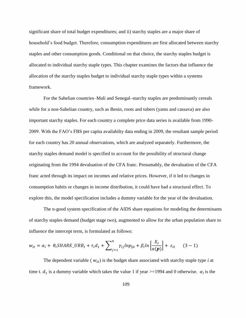
109
significant share of total budget expenditures; and ii) starchy staples are a major share of
household’s food budget. Therefore, consumption expenditures are first allocated between starchy
staples and other consumption goods. Conditional on that choice, the starchy staples budget is
allocated to individual starchy staple types. This chapter examines the factors that influence the
allocation of the starchy staples budget to individual starchy staple types within a systems
framework.
For the Sahelian countries–Mali and Senegal–starchy staples are predominantly cereals
while for a non-Sahelian country, such as Benin, roots and tubers (yams and cassava) are also
important starchy staples. For each country a complete price data series is available from 1990-
2009. With the FAO’s FBS per capita availabilty data ending in 2009, the resultant sample period
for each country has 20 annual observations, which are analyzed separately. Furthermore, the
starchy staples demand model is specified to account for the possibility of structural change
originating from the 1994 devaluation of the CFA franc. Presumably, the devaluation of the CFA
franc acted through its impact on incomes and relative prices. However, if it led to changes in
consumption habits or changes in income distribution, it could have had a structural effect. To
explore this, the model specification includes a dummy variable for the year of the devaluation.
The n-good system specification of the AIDS share equations for modeling the determinants
of starchy staples demand (budget stage two), augmented to allow for the urban population share to
influence the intercept term, is formulated as follows:
𝑤𝑖𝑡 = 𝛼𝑖 + 𝜃𝑖𝑆𝐻𝐴𝑅𝐸_𝑈𝑅𝐵𝑡 + 𝜏𝑖𝑑1 + ∑ 𝛾𝑖𝑗𝑙𝑛𝑝jit
𝑛
𝑗=1+ 𝛽𝑖𝑙𝑛 [
𝑋𝑡
𝑎(𝒑)] + 휀𝑖𝑡 (3 − 1)
The dependent variable ( 𝑤𝑖𝑡) is the budget share associated with starchy staple type 𝑖 ̇at
time t. 𝑑1 is a dummy variable which takes the value 1 if year >=1994 and 0 otherwise. 𝛼𝑖 is the
110
constant coefficient in the 𝑖̇th share equation, and 𝛾𝑖𝑗 is the slope coefficient associated with the jth
starchy staple type in the 𝑖̇th share equation. 𝑝jit is the normalized real price of starchy staple type j
in the share equation for starchy staple type 𝑖̇ at time t. 𝑋𝑡 is the total per capita expenditure on the
system of starchy staples given by 𝑋𝑡 = ∑ 𝑝𝑖𝑡𝑞𝑖𝑡𝑛𝑖=1 , where qit is the annual apparent per capita
consumption of the 𝑖̇th starchy staple type at time t, and 𝑝𝑖𝑡 is the normalized annual real price for
starchy staple type 𝑖 ̇at time t. p is a vector of normalized real prices, a (p) is a function that is
homogenous of degree one in prices, and lna(p) is specified as the translog equation:
ln 𝑎(𝑝) = 𝛼0 + ∑ 𝛼𝑖𝑙𝑛𝑝𝑖𝑡
𝑛
𝑖=1
+1
2∑ ∑ 𝛾𝑖𝑗
𝑛
𝑗=1
𝑛
𝑖=1
𝑙𝑛𝑝𝑖𝑡𝑙𝑛𝑝𝑗𝑡 (3 − 2)
Where i = 1…n denote commodities.
The translog price index in equation (3-2) is non-linear, thereby posing some difficulties
when aggregate annual time-series data are used. As a result, most studies employ a linear
approximation to the non-linear price index. The most usual approximation to the translog
aggregator function a(p) in the AIDS model has been the Stone price index suggested by Deaton
and Muellbauer (1980). Moschini (1995), in the context of the AIDS, showed that employing
Stone’s price index (ln 𝐏∗ = ∑ 𝑤𝑖𝑡𝑙𝑛𝑝𝑖𝑡𝑛𝑖=1 ) in place of a(p) can seriously bias elasticity estimates
partly because this price index is influenced by changes in units of measurement. He therefore
suggested using the following alternative price indices: the Törnqvist price index [log 𝑃𝑇 =
0.5 ∑ (𝑤𝑖𝑡 + 𝑤𝑖𝑡0 )𝑙𝑜𝑔 (𝑃𝑖𝑡 𝑃𝑖𝑡
0⁄𝑛𝑖=1 )], the loglinear analogue of the Paasche price index–also known as
the “corrected” Stone price index [log 𝑃𝑠 = ∑ 𝑤𝑖𝑡𝑙𝑜𝑔 (𝑃𝑖𝑡 𝑃𝑖𝑡0⁄𝑛
𝑖=1 )], and the loglinear analogue of
the Laspeyres price index [ln P𝐋 = ∑ 𝑤𝑖𝑡0 𝑙𝑛𝑝𝑖𝑡
𝑛𝑖=1 ] , all of which are exact for a linearly
homogeneous Cobb–Douglas aggregator function (Diewert 1976) and invariant to changes in units.
111
For the purpose of this study, the translog price aggregator, a(p), is approximated by the Laspeyres
price index:ln PL = ∑ 𝑤𝑖𝑡0 𝑙𝑛𝑝𝑖𝑡
𝑛𝑖=1 , where 𝑤𝑖𝑡
0 is the share of the ith commodity in the base period.
Owing to its simplicity, LA-AIDS is very popular in empirical studies.
The theoretical restrictions of homogeneity, adding up and symmetry are imposed on the
parameters to ensure integrability of the demand system. Adding-up requires that expenditure
shares sum to one (i.e., ∑ 𝑤𝑖𝑛𝑖=1 = 1 ), and can be expressed in terms of model parameters as:
∑ 𝛼𝑖 = 0,
𝑛
𝑖=1
∑ 𝛽𝑖 = 0,
𝑛
𝑖=1
∑ 𝛾𝑖𝑗 = 0,
𝑛
𝑖=1
∀𝑗
An additional requirement for adding up is that
∑ 𝜃𝑖
𝑛
𝑖=1
= 0
Hicksian demands are homogenous of degree zero in prices, which implies
∑ 𝛾𝑖𝑗
𝑛
𝑗=1
= 0 ∀𝑗
The Slutsky symmetry restriction requires that
𝛾𝑖𝑗 = 𝛾𝑗𝑖 = 0 ∀ i, j
These restrictions (adding-up, homogeneity, and symmetry) are imposed during estimation.
Negativity is not automatically introduced, but by estimating all the compensated own-price
elasticities one can test for their negativity.
The expenditure elasticity, which varies depending on the type of good (normal or inferior),
for good i̇ is given as:
𝜂𝑖 =𝛽𝑖
𝑤𝑖 + 1 (3 − 3)
112
In equation (3-3) parameter 𝛽𝑖determines the effect of a change in total per capita starchy-
staple expenditure on the budget share of starchy-staple type 𝑖 ̇and determines whether this good is
normal or inferior.
The Marshallian (uncompensated) own-price and cross-price elasticities are calculated in the
following manner:
휀𝑖𝑗 =𝛾𝑖𝑗
𝑤𝑖−
𝛽𝑖
𝑤𝑖𝑤𝑗
0 − 𝛿𝑖𝑗 (3 – 4)
Where 𝛿𝑖𝑗 is the Kronecker delta equaling 1 if i=j and 0 otherwise.
In the LA-AIDS model the Hicksian or compensated price elasticities are derived using the Slutsky
equation and are given by:
휀𝑖𝑗∗ = 휀𝑖𝑗 + 𝑤𝑗𝜂𝑖 (3 − 5)
It is well known that most economic time series data are very persistent, suggesting the
possibility of non-stationary behavior. The presence of unit roots may invalidate the asymptotic
distribution of estimators and influence elasticity estimates and their standard errors. Consequently,
the appropriate model specification depends on the time-series properties of the data. The time-
series properties of the data are investigated to determine whether long-run relationships are
economically meaningful or not. A formal test for unit roots is performed on all the data series used
in the estimation. The unit roots test is first carried out with the pioneering Augmented Dickey-
Fuller (ADF) test proposed in 1981. Wang and Tomek (2004) argue that the results of unit root tests
are conditional on the remaining specification of the right hand side of the estimation equation —
with and without a linear deterministic trend; and the length of lags, if any, to include. The tests
113
here were conducted with and without a trend and on the natural logarithm of deflated26 prices, the
natural logarithm of starchy staples expenditure and the commodity budget shares. The number of
lags included in the test was chosen so as to make the error term white noise. Due to the criticism of
the ADF test – its low statistical power to reject a unit root, an alternative test–the Phillips-Perron
(PP) test, proposed in 1988 and known for better finite sample properties than the ADF test—is also
employed to check the robustness of the ADF results. The ADF and PP test for unit roots have non-
stationarity as the null hypothesis. The difficulty of rejecting this hypothesis has been pointed in the
literature. Hence to further test for the robustness of the ADF and PP results, the KPSS
(Kwiatkowski, et al. 1992) test for unit roots that has stationarity as the null hypothesis is also
applied. A similar unit roots testing approach is used in the data for the threee countries covered in
this chapter.
According to theory, regression of two variables that are integrated of order one I(1)27 but
are not cointegrated results in a spurious regression. A cointegrating relationship exists when a
linear combination of two or more I(1) variables results in residuals that are I(0)–implying that
although the variables are non-stationary, a linear combination of them is stationary, thus
generating an equilibrium relationship in the long-run. Karagiannis et al. (2000) observe that it is
also possible to have a cointegrated regression even though the variables of interest have different
time-series properties and thus, a different order of integration. According to the Granger
representation theorem, a linear combination of series with a different orders of integration may still
be a cointegrating regression. He notes further that if cointegration cannot be established for at least
26 Using the GDP deflator. 27 Such that first-differencing makes the variables stationary.
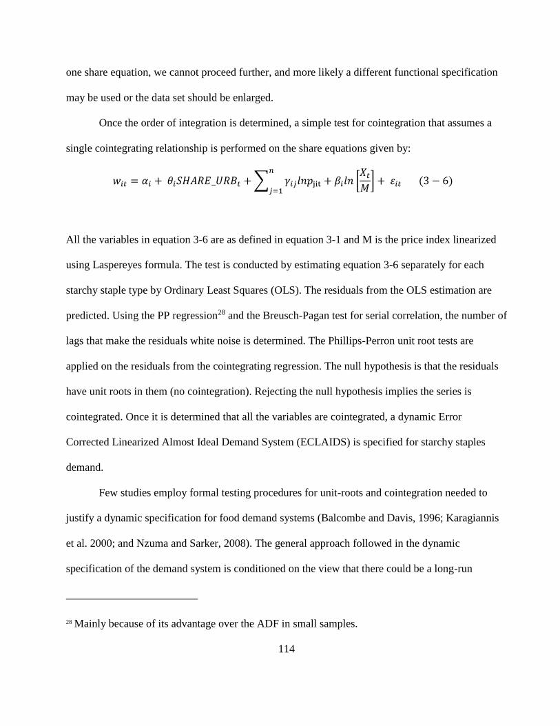
114
one share equation, we cannot proceed further, and more likely a different functional specification
may be used or the data set should be enlarged.
Once the order of integration is determined, a simple test for cointegration that assumes a
single cointegrating relationship is performed on the share equations given by:
𝑤𝑖𝑡 = 𝛼𝑖 + 𝜃𝑖𝑆𝐻𝐴𝑅𝐸_𝑈𝑅𝐵𝑡 + ∑ 𝛾𝑖𝑗𝑙𝑛𝑝jit
𝑛
𝑗=1+ 𝛽𝑖𝑙𝑛 [
𝑋𝑡
𝑀] + 휀𝑖𝑡 (3 − 6)
All the variables in equation 3-6 are as defined in equation 3-1 and M is the price index linearized
using Laspereyes formula. The test is conducted by estimating equation 3-6 separately for each
starchy staple type by Ordinary Least Squares (OLS). The residuals from the OLS estimation are
predicted. Using the PP regression28 and the Breusch-Pagan test for serial correlation, the number of
lags that make the residuals white noise is determined. The Phillips-Perron unit root tests are
applied on the residuals from the cointegrating regression. The null hypothesis is that the residuals
have unit roots in them (no cointegration). Rejecting the null hypothesis implies the series is
cointegrated. Once it is determined that all the variables are cointegrated, a dynamic Error
Corrected Linearized Almost Ideal Demand System (ECLAIDS) is specified for starchy staples
demand.
Few studies employ formal testing procedures for unit-roots and cointegration needed to
justify a dynamic specification for food demand systems (Balcombe and Davis, 1996; Karagiannis
et al. 2000; and Nzuma and Sarker, 2008). The general approach followed in the dynamic
specification of the demand system is conditioned on the view that there could be a long-run
28 Mainly because of its advantage over the ADF in small samples.
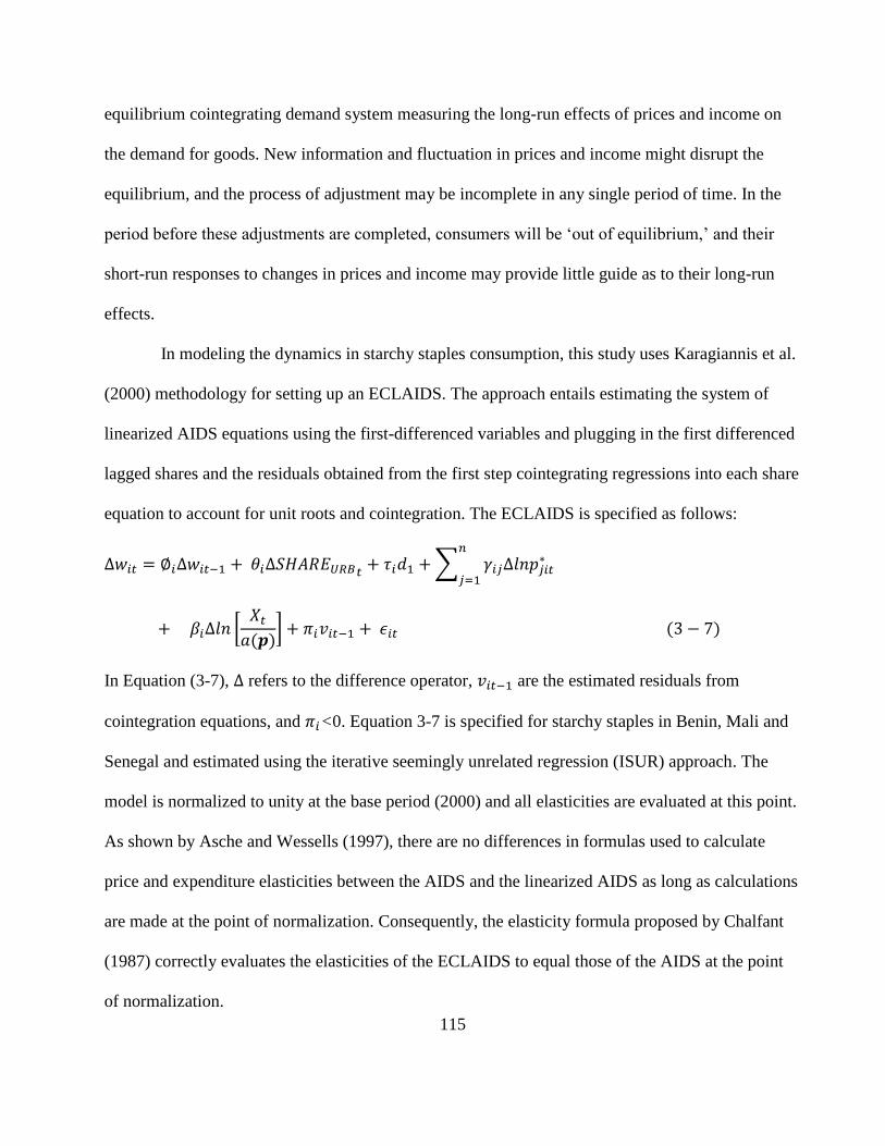
115
equilibrium cointegrating demand system measuring the long-run effects of prices and income on
the demand for goods. New information and fluctuation in prices and income might disrupt the
equilibrium, and the process of adjustment may be incomplete in any single period of time. In the
period before these adjustments are completed, consumers will be ‘out of equilibrium,’ and their
short-run responses to changes in prices and income may provide little guide as to their long-run
effects.
In modeling the dynamics in starchy staples consumption, this study uses Karagiannis et al.
(2000) methodology for setting up an ECLAIDS. The approach entails estimating the system of
linearized AIDS equations using the first-differenced variables and plugging in the first differenced
lagged shares and the residuals obtained from the first step cointegrating regressions into each share
equation to account for unit roots and cointegration. The ECLAIDS is specified as follows:
∆𝑤𝑖𝑡 = ∅𝑖∆𝑤𝑖𝑡−1 + 𝜃𝑖∆𝑆𝐻𝐴𝑅𝐸𝑈𝑅𝐵𝑡+ 𝜏𝑖𝑑1 + ∑ 𝛾𝑖𝑗∆𝑙𝑛𝑝𝑗𝑖𝑡
∗𝑛
𝑗=1
+ 𝛽𝑖∆𝑙𝑛 [𝑋𝑡
𝑎(𝒑)] + 𝜋𝑖𝑣𝑖𝑡−1 + 𝜖𝑖𝑡 (3 − 7)
In Equation (3-7), ∆ refers to the difference operator, 𝑣𝑖𝑡−1 are the estimated residuals from
cointegration equations, and 𝜋𝑖<0. Equation 3-7 is specified for starchy staples in Benin, Mali and
Senegal and estimated using the iterative seemingly unrelated regression (ISUR) approach. The
model is normalized to unity at the base period (2000) and all elasticities are evaluated at this point.
As shown by Asche and Wessells (1997), there are no differences in formulas used to calculate
price and expenditure elasticities between the AIDS and the linearized AIDS as long as calculations
are made at the point of normalization. Consequently, the elasticity formula proposed by Chalfant
(1987) correctly evaluates the elasticities of the ECLAIDS to equal those of the AIDS at the point
of normalization.
116
3.5. Findings
This section presents findings from the analysis of the determinants of aggregate demand for
starchy staples in Senegal, Benin, and Mali. In particular, it provides estimates of the relationship
between structural factors expected to influence consumption (urbanization and per capita incomes)
as well as estimates of price and income elasticities of starchy staples demand for each major
starchy staple type. The results are presented by country.
3.5.1. Determinants of Starchy Staples Demand – Senegal
The analysis of trends in per capita food availability in Senegal (Chapter 2) revealed an overall
decrease of 14 kg/year in the per capita availability of cereals and an increase in the supply of
starchy roots and tubers (R&T) of about 18 kg/capita between the period 1980/85 and 2004/2009. A
breakdown of the cereals and starchy R&T food groups by individual commodities revealed a
growth in the per capita availability of rice and maize at the expense of millet and sorghum in the
cereals food group. Cassava availability per capita also rose during the study period. However, it
stayed relatively low compared to grains. This sub-section therefore aims to examine if there is any
statistical relationship between above-mentioned descriptive trends and the factors hypothesized to
influence aggregate level demand shifts (urbanization, relative prices, and growth in per capita
incomes). In the absence of good time-series R&T price data, the analysis of the determinants of
starchy staple demand in Senegal in this chapter is limited to cereals (rice, maize, millet, and
sorghum).
Table 3-1 presents summary statistics of the data used in estimating aggregate demand for
Senegal. Average budget shares per starchy staple type in the study period were 48% for rice; 30%
for millet; 12% for maize, and 10% for sorghum. The urban population share rose only by 3.64% in
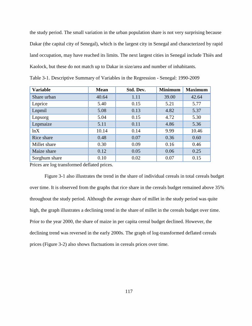
117
the study period. The small variation in the urban population share is not very surprising because
Dakar (the capital city of Senegal), which is the largest city in Senegal and characterized by rapid
land occupation, may have reached its limits. The next largest cities in Senegal include Thiès and
Kaolock, but these do not match up to Dakar in size/area and number of inhabitants.
Table 3-1. Descriptive Summary of Variables in the Regression - Senegal: 1990-2009
Variable Mean Std. Dev. Minimum Maximum
Share urban 40.64 1.11 39.00 42.64
Lnprice 5.40 0.15 5.21 5.77
Lnpmil 5.08 0.13 4.82 5.37
Lnpsorg 5.04 0.15 4.72 5.30
Lnpmaize 5.11 0.11 4.86 5.36
lnX 10.14 0.14 9.99 10.46
Rice share 0.48 0.07 0.36 0.60
Millet share 0.30 0.09 0.16 0.46
Maize share 0.12 0.05 0.06 0.25
Sorghum share 0.10 0.02 0.07 0.15
Prices are log transformed deflated prices.
Figure 3-1 also illustrates the trend in the share of individual cereals in total cereals budget
over time. It is observed from the graphs that rice share in the cereals budget remained above 35%
throughout the study period. Although the average share of millet in the study period was quite
high, the graph illustrates a declining trend in the share of millet in the cereals budget over time.
Prior to the year 2000, the share of maize in per capita cereal budget declined. However, the
declining trend was reversed in the early 2000s. The graph of log-transformed deflated cereals
prices (Figure 3-2) also shows fluctuations in cereals prices over time.
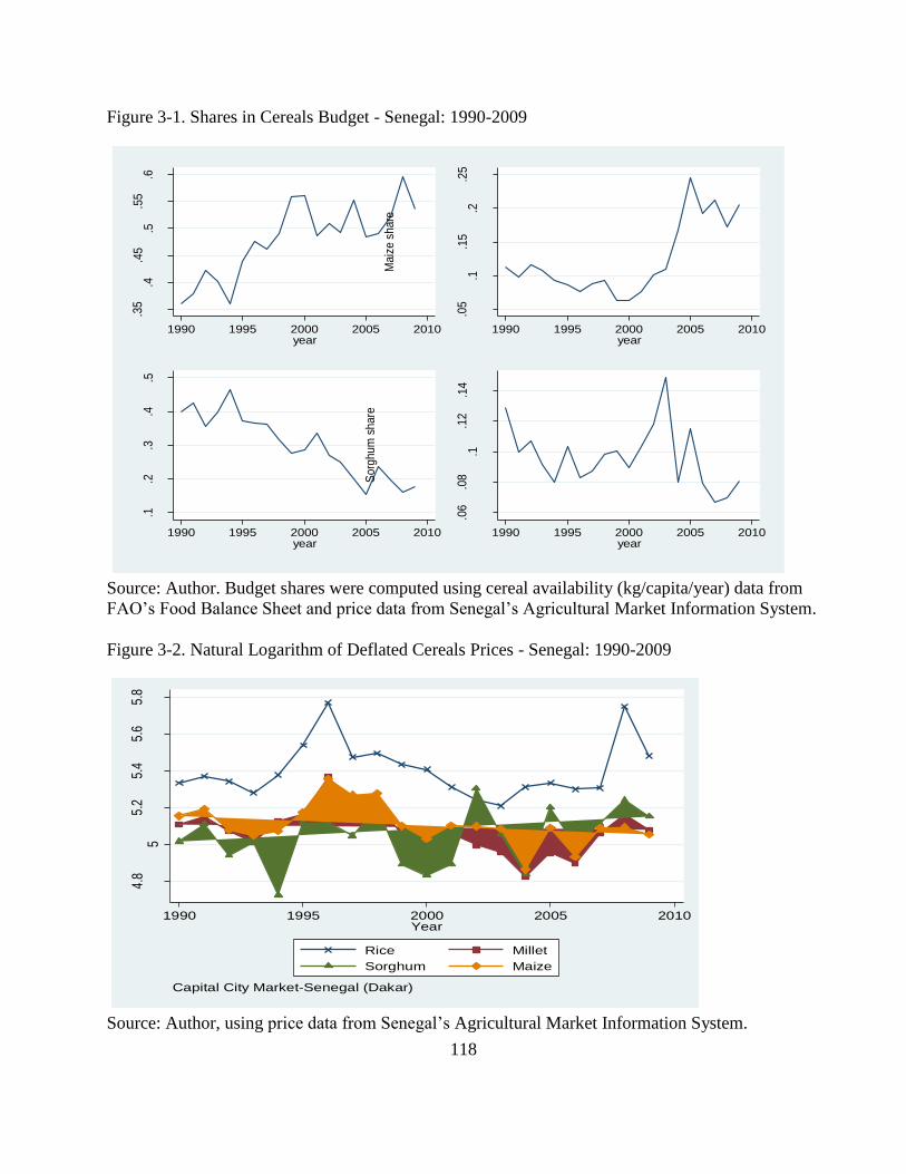
118
Figure 3-1. Shares in Cereals Budget - Senegal: 1990-2009
Source: Author. Budget shares were computed using cereal availability (kg/capita/year) data from
FAO’s Food Balance Sheet and price data from Senegal’s Agricultural Market Information System.
Figure 3-2. Natural Logarithm of Deflated Cereals Prices - Senegal: 1990-2009
Source: Author, using price data from Senegal’s Agricultural Market Information System.
.35
.4.4
5.5
.55
.6
rice
share
1990 1995 2000 2005 2010year
.05
.1.1
5.2
.25
Maiz
e s
hare
1990 1995 2000 2005 2010year
.1.2
.3.4
.5
Mill
et S
hare
1990 1995 2000 2005 2010year
.06
.08
.1.1
2.1
4
Sorg
hum
share
1990 1995 2000 2005 2010year
4.8
55.
25.
45.
65.
8
Loga
rithm
of D
efla
ted
Pric
es
1990 1995 2000 2005 2010Year
Rice Millet
Sorghum Maize
Capital City Market-Senegal (Dakar)
119
An examination of the correlation coefficient between the urban population share and
starchy staples budget shares reveals a strong positive relationship with the rice budget share (0.78)
and with the maize budget share (0.71). Millet and sorghum on the other hand were found to be
negatively correlated with the urban population share with correlation coefficients of -0.92 and -
0.34 respectively. These relationships are not surprising because millet is a basic rural food in
Senegal, although over time, rice has deeply penetrated rural markets and diets.
The results of the ADF and PP test for non-stationarity of the variables in the demand
estimation are reported in Table A3-1 in Appendix (case with trend) and Table A3-2 in Appendix
(the case without trend). In both cases, results suggest most variables are stationary and few are
non-stationary in levels. First differencing also fails to make all the variables stationary when the
ADF test is applied in the case with and without trend. Based on a PP test, a unit root is rejected at a
5% significance level for some of the variables in the case with and without a trend. Performing the
PP-test on first-differenced variables, non-stationarity is rejected at a 1% level of significance for all
the variables in the case with and without trend.29 Using the KPSS test for unit roots (Appendix,
Tables A3-3 and A3-4), we reject the null of stationarity in some of the variables to be used in the
demand estimation in the case with and without trend. When all the variables are treated as non-
stationary in levels and first differenced, we do not reject stationarity in the case with and without
trend in all the variables to be used in the estimation. Thus, in all three tests we do not reject
stationarity in some of the variables in levels. The inconclusive result of the unit root tests on the
variables in levels supports existing arguments on the low power of unit root tests in small samples.
29 Since a trend in levels becomes a constant in first differences, no trend needs to be included here,
making the option of first differencing with no trend more appropriate.
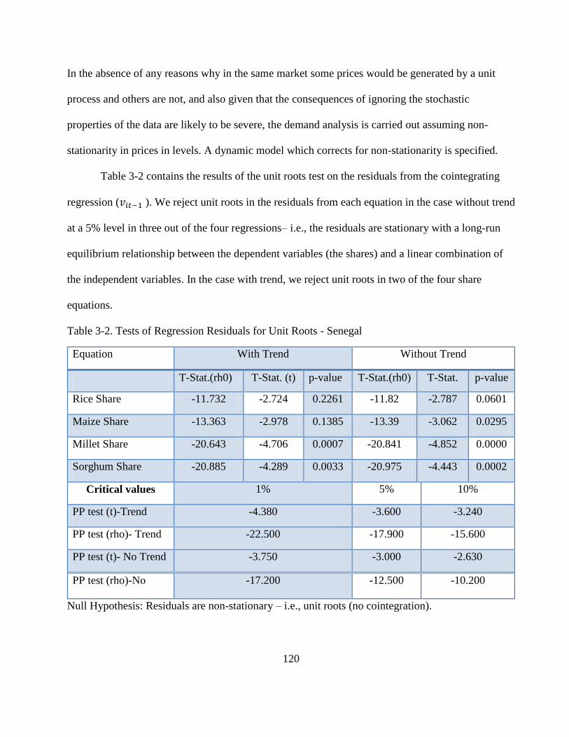
120
In the absence of any reasons why in the same market some prices would be generated by a unit
process and others are not, and also given that the consequences of ignoring the stochastic
properties of the data are likely to be severe, the demand analysis is carried out assuming non-
stationarity in prices in levels. A dynamic model which corrects for non-stationarity is specified.
Table 3-2 contains the results of the unit roots test on the residuals from the cointegrating
regression (𝑣𝑖𝑡−1 ). We reject unit roots in the residuals from each equation in the case without trend
at a 5% level in three out of the four regressions– i.e., the residuals are stationary with a long-run
equilibrium relationship between the dependent variables (the shares) and a linear combination of
the independent variables. In the case with trend, we reject unit roots in two of the four share
equations.
Table 3-2. Tests of Regression Residuals for Unit Roots - Senegal
Equation With Trend Without Trend
T-Stat.(rh0) T-Stat. (t) p-value T-Stat.(rh0) T-Stat.
(t)
p-value
Rice Share -11.732 -2.724 0.2261 -11.82 -2.787 0.0601
Maize Share -13.363 -2.978 0.1385 -13.39 -3.062 0.0295
Millet Share -20.643 -4.706 0.0007 -20.841 -4.852 0.0000
Sorghum Share -20.885 -4.289 0.0033 -20.975 -4.443 0.0002
Critical values 1% 5% 10%
PP test (t)-Trend -4.380 -3.600 -3.240
PP test (rho)- Trend -22.500 -17.900 -15.600
PP test (t)- No Trend -3.750 -3.000 -2.630
PP test (rho)-No
Trend
-17.200 -12.500 -10.200
Null Hypothesis: Residuals are non-stationary – i.e., unit roots (no cointegration).
121
Having established the existence of a long run equilibrium relationship, an ECLAIDS model
(equation 3-7) is estimated for the four major grain types (rice, maize, millet, and sorghum)
consumed in Senegal. The model was estimated with and without the dummy variable that captures
the effect of any structural change in consumption habits due to devaluation. The inclusion of the
dummy variable failed to provide any noticeable improvement in the estimated parameters. As a
result, the reported parameter estimates are from the model without the dummy for devaluation.
Table 3-3 contains the estimated parameters of the ECLAIDS for cereals demand in Senegal 1990-
2009. The estimated parameters of the error correction terms (𝜋𝑖) are all statistically significant and
have the correct signs, indicating that deviations from long-run equilibrium are corrected within the
time period. It is also worth noting that the significance of the error correction terms in SUR
estimates is consistent with the previously obtained results of cointegration analysis. The estimated
R-squares are 74% for rice, 72% for millet, and 30% for sorghum. Furthermore, the log of per
capita starchy staples expenditure and the urban population share are not statistically significant in
any of the budget share equations, meaning that starchy staples expenditure behavior as well as the
urban population shares are influenced neither by changes in aggregate expenditures on starchy
staples per capita or growth in urban population shares when aggregate consumption data are
considered. However, this may be an inappropriate conclusion given that the distribution of income
across different consumers and/or by place of residence may be a more critical determinant of
cereals consumption than national level per capita expenditures. Furthermore, the urban population
did not change much (increased by 3.64%) in Senegal during the study period. This may explain
why urbanization is not statistically significant in the starchy staple demand model.
As shown by Asche and Wessells (1997), there are no differences in formulas used to
calculate price and expenditure elasticities between the AIDS and the linearized AIDS as long as
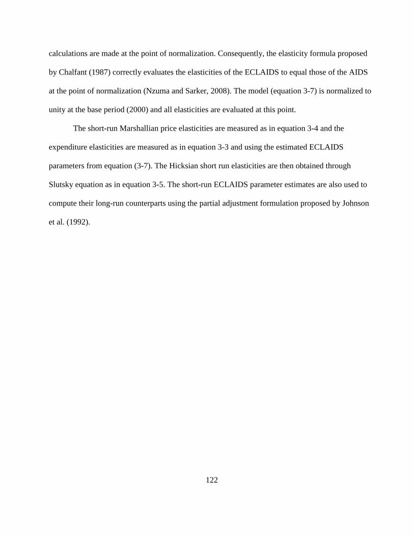
122
calculations are made at the point of normalization. Consequently, the elasticity formula proposed
by Chalfant (1987) correctly evaluates the elasticities of the ECLAIDS to equal those of the AIDS
at the point of normalization (Nzuma and Sarker, 2008). The model (equation 3-7) is normalized to
unity at the base period (2000) and all elasticities are evaluated at this point.
The short-run Marshallian price elasticities are measured as in equation 3-4 and the
expenditure elasticities are measured as in equation 3-3 and using the estimated ECLAIDS
parameters from equation (3-7). The Hicksian short run elasticities are then obtained through
Slutsky equation as in equation 3-5. The short-run ECLAIDS parameter estimates are also used to
compute their long-run counterparts using the partial adjustment formulation proposed by Johnson
et al. (1992).
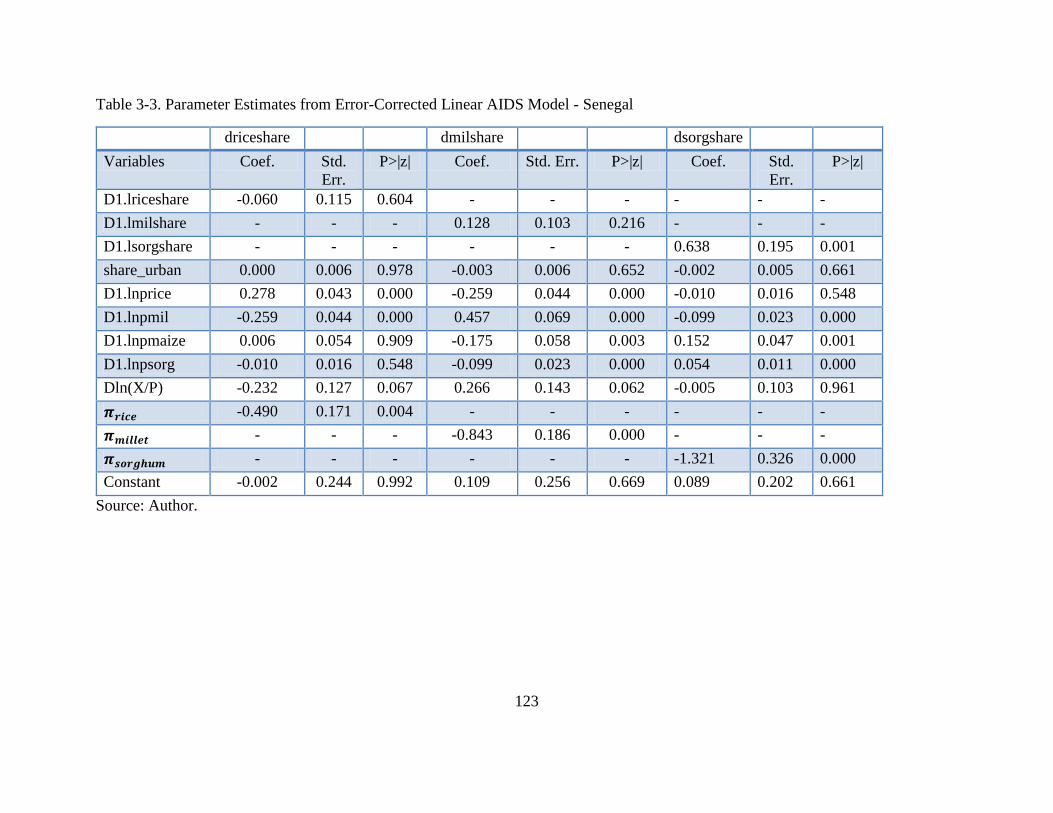
123
Table 3-3. Parameter Estimates from Error-Corrected Linear AIDS Model - Senegal
driceshare dmilshare dsorgshare
Variables Coef. Std.
Err.
P>|z| Coef. Std. Err. P>|z| Coef. Std.
Err.
P>|z|
D1.lriceshare -0.060 0.115 0.604 - - - - - -
D1.lmilshare - - - 0.128 0.103 0.216 - - -
D1.lsorgshare - - - - - - 0.638 0.195 0.001
share_urban 0.000 0.006 0.978 -0.003 0.006 0.652 -0.002 0.005 0.661
D1.lnprice 0.278 0.043 0.000 -0.259 0.044 0.000 -0.010 0.016 0.548
D1.lnpmil -0.259 0.044 0.000 0.457 0.069 0.000 -0.099 0.023 0.000
D1.lnpmaize 0.006 0.054 0.909 -0.175 0.058 0.003 0.152 0.047 0.001
D1.lnpsorg -0.010 0.016 0.548 -0.099 0.023 0.000 0.054 0.011 0.000
Dln(X/P) -0.232 0.127 0.067 0.266 0.143 0.062 -0.005 0.103 0.961
𝝅𝒓𝒊𝒄𝒆 -0.490 0.171 0.004 - - - - - -
𝝅𝒎𝒊𝒍𝒍𝒆𝒕 - - - -0.843 0.186 0.000 - - -
𝝅𝒔𝒐𝒓𝒈𝒉𝒖𝒎 - - - - - - -1.321 0.326 0.000
Constant -0.002 0.244 0.992 0.109 0.256 0.669 0.089 0.202 0.661
Source: Author.
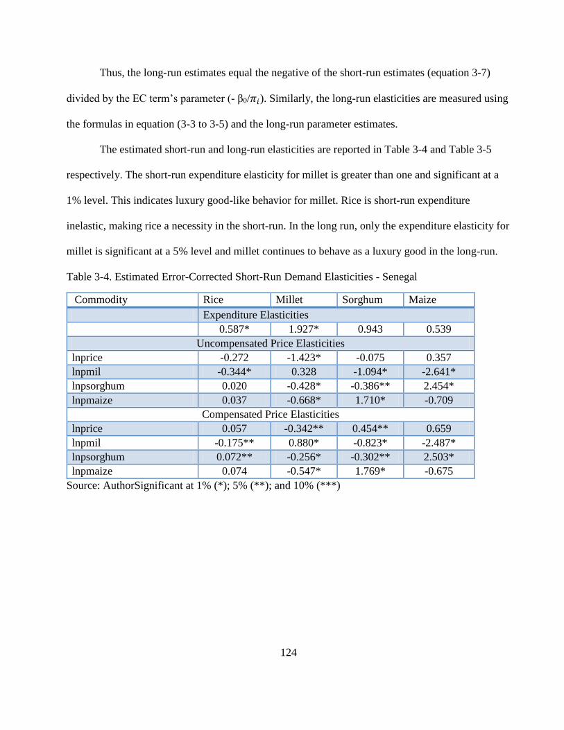
124
Thus, the long-run estimates equal the negative of the short-run estimates (equation 3-7)
divided by the EC term’s parameter (- β0/𝜋𝑖). Similarly, the long-run elasticities are measured using
the formulas in equation (3-3 to 3-5) and the long-run parameter estimates.
The estimated short-run and long-run elasticities are reported in Table 3-4 and Table 3-5
respectively. The short-run expenditure elasticity for millet is greater than one and significant at a
1% level. This indicates luxury good-like behavior for millet. Rice is short-run expenditure
inelastic, making rice a necessity in the short-run. In the long run, only the expenditure elasticity for
millet is significant at a 5% level and millet continues to behave as a luxury good in the long-run.
Table 3-4. Estimated Error-Corrected Short-Run Demand Elasticities - Senegal
Commodity Rice Millet Sorghum Maize
Expenditure Elasticities
0.587* 1.927* 0.943 0.539
Uncompensated Price Elasticities
lnprice -0.272 -1.423* -0.075 0.357
lnpmil -0.344* 0.328 -1.094* -2.641*
lnpsorghum 0.020 -0.428* -0.386** 2.454*
lnpmaize 0.037 -0.668* 1.710* -0.709
Compensated Price Elasticities
lnprice 0.057 -0.342** 0.454** 0.659
lnpmil -0.175** 0.880* -0.823* -2.487*
lnpsorghum 0.072** -0.256* -0.302** 2.503*
lnpmaize 0.074 -0.547* 1.769* -0.675
Source: AuthorSignificant at 1% (*); 5% (**); and 10% (***)
125
Table 3-5. Senegal: Estimated Error-Corrected Long-Run Demand Elasticities
Commodity Rice Millet Sorghum Maize
Expenditure Elasticities
0.157 2.099* 0.957 3.556
Uncompensated Price Elasticities
lnprice 0.485 -1.687* -0.057 -1.233
lnpmil -0.701* 0.575 -0.828** -4.023**
lnpsorghum 0.040 -0.507* -0.536* 1.598**
lnpmaize 0.076 -0.792** 1.294* 0.101
Compensated Price Elasticities
lnprice 0.573 -0.510*** 0.480* 0.761
lnpmil -0.656*** 1.177** -0.553*** -3.002**
lnpsorghum 0.054 -0.320** -0.450* 1.916*
lnpmaize 0.086 -0.660** 1.354* 0.326
Source: Author
Note: Significant at 1% (*); 5% (**); and 10% (***)
With the exception of millet, all the short-run own-price Marshallian elasticities are
negative, and thus the corresponding demand curves are downward sloping (see Table 3.4).
However, only the uncompensated short-run own-price elasticity of sorghum is statistically
significant at a 5%, and sorghum is found to be own-price inelastic in the short-run. When the long-
run own-price Marshallian elasticities are considered, sorghum remains price inelastic and
statistically significant, with long-run Marshallian own-price elasticity greater than the short-run.
Not all short-run own-price Hicksian elasticities are negative as expected. The positive and
statistically significant compensated demand curves for millet in both the short-run and the long-run
are not theoretically reasonable, and therefore warrant further investigation.
The short-run Hicksian cross-price elasticities (Table 3-4) reveal a relationship of
complementarity between millet and rice in the short-run; and a relationship of substitution between
sorghum and rice in the short-run, and these relationships are statistically significant at a 5% level.
For instance, in the short-run, a 1% increase in the price of sorghum will result in a compensated
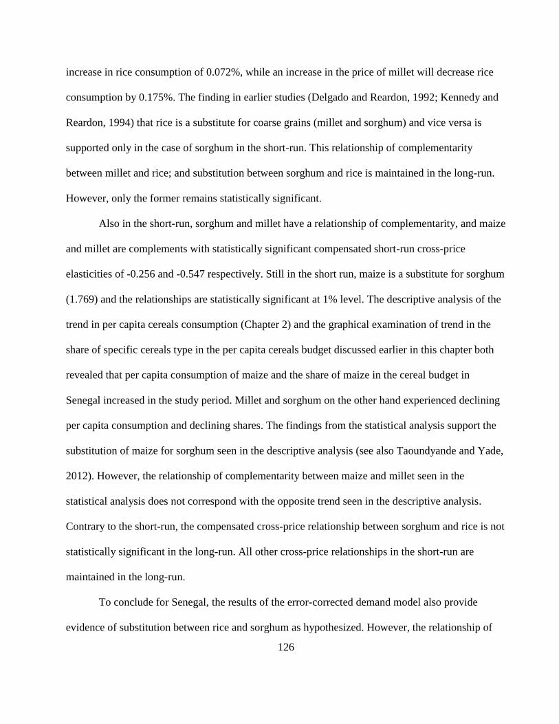
126
increase in rice consumption of 0.072%, while an increase in the price of millet will decrease rice
consumption by 0.175%. The finding in earlier studies (Delgado and Reardon, 1992; Kennedy and
Reardon, 1994) that rice is a substitute for coarse grains (millet and sorghum) and vice versa is
supported only in the case of sorghum in the short-run. This relationship of complementarity
between millet and rice; and substitution between sorghum and rice is maintained in the long-run.
However, only the former remains statistically significant.
Also in the short-run, sorghum and millet have a relationship of complementarity, and maize
and millet are complements with statistically significant compensated short-run cross-price
elasticities of -0.256 and -0.547 respectively. Still in the short run, maize is a substitute for sorghum
(1.769) and the relationships are statistically significant at 1% level. The descriptive analysis of the
trend in per capita cereals consumption (Chapter 2) and the graphical examination of trend in the
share of specific cereals type in the per capita cereals budget discussed earlier in this chapter both
revealed that per capita consumption of maize and the share of maize in the cereal budget in
Senegal increased in the study period. Millet and sorghum on the other hand experienced declining
per capita consumption and declining shares. The findings from the statistical analysis support the
substitution of maize for sorghum seen in the descriptive analysis (see also Taoundyande and Yade,
2012). However, the relationship of complementarity between maize and millet seen in the
statistical analysis does not correspond with the opposite trend seen in the descriptive analysis.
Contrary to the short-run, the compensated cross-price relationship between sorghum and rice is not
statistically significant in the long-run. All other cross-price relationships in the short-run are
maintained in the long-run.
To conclude for Senegal, the results of the error-corrected demand model also provide
evidence of substitution between rice and sorghum as hypothesized. However, the relationship of
127
complementarity between rice and millet in both the short-run and long-run are contrary to findings
from earlier studies that rice is a substitute for coarse grains. Hence, the hypothesis that rice is a
substitute for coarse grains (millet and sorghum) is only partially accepted in Senegal. The dynamic
specification (long-run and short-run) of cereals demand in Senegal provide evidence of
substitution of maize for sorghum and complementarity between maize and millet. Rice and maize
have the same behavior towards millet and sorghum. The finding that millet is expenditure elastic is
contrary to the expectation that as per capita income (and hence the budget share allocated to
starchy staples) increases, the share of the budget allocated to coarse grains will decrease and that to
rice will increase.
3.5.2. Determinants of Starchy Staples Demand – Benin
Table 3-6 contains a descriptive summary of the data used to estimate aggregate demand of starchy
staples for Benin. Millet and sorghum combined represent less than 5% of the starchy staple food
budget. As a result, due to small size of the sample and also to avoid degrees of freedom problems,
both were left out of the analysis of starchy staples demand in Benin. Starchy staples for Benin in
this chapter include rice, maize, yams, and cassava. Cassava alone represents an average of 53% of
the starchy staple budget, yams represent 30%, rice30 represents 4%; and maize represents 14%.
30 Imported rice prices are used since almost all of the rice available for consumption in Benin comes from imports.
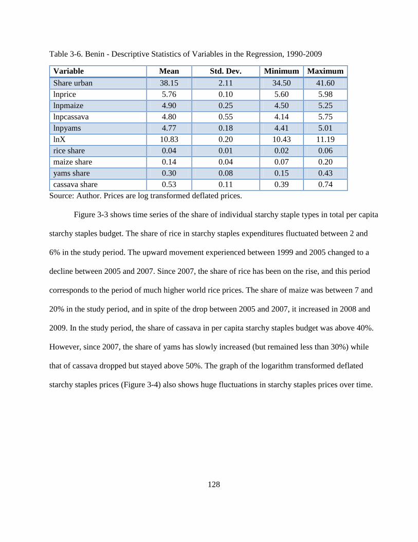
128
Table 3-6. Benin - Descriptive Statistics of Variables in the Regression, 1990-2009
Variable Mean Std. Dev. Minimum Maximum
Share urban 38.15 2.11 34.50 41.60
lnprice 5.76 0.10 5.60 5.98
lnpmaize 4.90 0.25 4.50 5.25
lnpcassava 4.80 0.55 4.14 5.75
lnpyams 4.77 0.18 4.41 5.01
lnX 10.83 0.20 10.43 11.19
rice share 0.04 0.01 0.02 0.06
maize share 0.14 0.04 0.07 0.20
yams share 0.30 0.08 0.15 0.43
cassava share 0.53 0.11 0.39 0.74
Source: Author. Prices are log transformed deflated prices.
Figure 3-3 shows time series of the share of individual starchy staple types in total per capita
starchy staples budget. The share of rice in starchy staples expenditures fluctuated between 2 and
6% in the study period. The upward movement experienced between 1999 and 2005 changed to a
decline between 2005 and 2007. Since 2007, the share of rice has been on the rise, and this period
corresponds to the period of much higher world rice prices. The share of maize was between 7 and
20% in the study period, and in spite of the drop between 2005 and 2007, it increased in 2008 and
2009. In the study period, the share of cassava in per capita starchy staples budget was above 40%.
However, since 2007, the share of yams has slowly increased (but remained less than 30%) while
that of cassava dropped but stayed above 50%. The graph of the logarithm transformed deflated
starchy staples prices (Figure 3-4) also shows huge fluctuations in starchy staples prices over time.
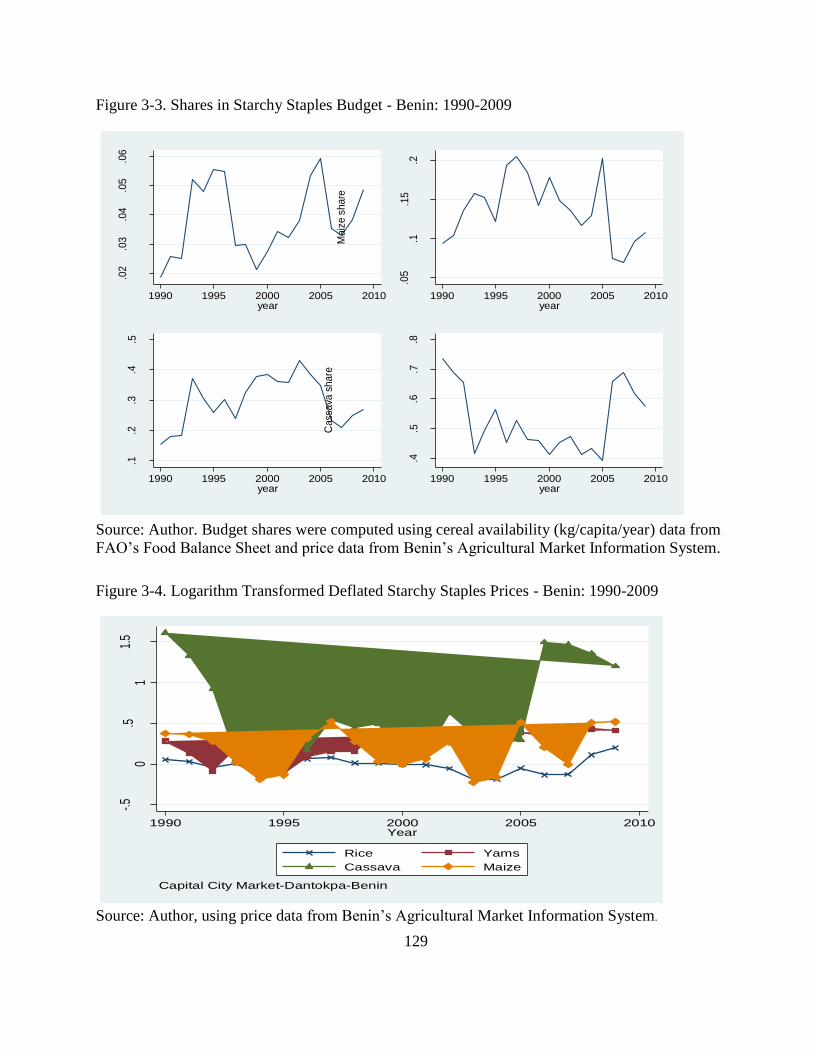
129
Figure 3-3. Shares in Starchy Staples Budget - Benin: 1990-2009
Source: Author. Budget shares were computed using cereal availability (kg/capita/year) data from
FAO’s Food Balance Sheet and price data from Benin’s Agricultural Market Information System.
Figure 3-4. Logarithm Transformed Deflated Starchy Staples Prices - Benin: 1990-2009
Source: Author, using price data from Benin’s Agricultural Market Information System.
.02
.03
.04
.05
.06
Ric
e s
hare
1990 1995 2000 2005 2010year
.05
.1.1
5.2
Maiz
e s
hare
1990 1995 2000 2005 2010year
.1.2
.3.4
.5
Yam
s sh
are
1990 1995 2000 2005 2010year
.4.5
.6.7
.8
Cass
ava
share
1990 1995 2000 2005 2010year
-.50
.51
1.5
Loga
rithm
of D
efla
ted
Pric
es
1990 1995 2000 2005 2010Year
Rice Yams
Cassava Maize
Capital City Market-Dantokpa-Benin
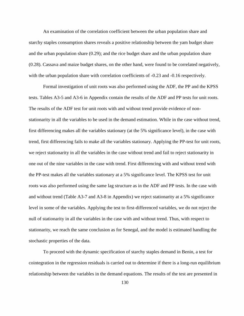
130
An examination of the correlation coefficient between the urban population share and
starchy staples consumption shares reveals a positive relationship between the yam budget share
and the urban population share (0.29); and the rice budget share and the urban population share
(0.28). Cassava and maize budget shares, on the other hand, were found to be correlated negatively,
with the urban population share with correlation coefficients of -0.23 and -0.16 respectively.
Formal investigation of unit roots was also performed using the ADF, the PP and the KPSS
tests. Tables A3-5 and A3-6 in Appendix contain the results of the ADF and PP tests for unit roots.
The results of the ADF test for unit roots with and without trend provide evidence of non-
stationarity in all the variables to be used in the demand estimation. While in the case without trend,
first differencing makes all the variables stationary (at the 5% significance level), in the case with
trend, first differencing fails to make all the variables stationary. Applying the PP-test for unit roots,
we reject stationarity in all the variables in the case without trend and fail to reject stationarity in
one out of the nine variables in the case with trend. First differencing with and without trend with
the PP-test makes all the variables stationary at a 5% significance level. The KPSS test for unit
roots was also performed using the same lag structure as in the ADF and PP tests. In the case with
and without trend (Table A3-7 and A3-8 in Appendix) we reject stationarity at a 5% significance
level in some of the variables. Applying the test to first-differenced variables, we do not reject the
null of stationarity in all the variables in the case with and without trend. Thus, with respect to
stationarity, we reach the same conclusion as for Senegal, and the model is estimated handling the
stochastic properties of the data.
To proceed with the dynamic specification of starchy staples demand in Benin, a test for
cointegration in the regression residuals is carried out to determine if there is a long-run equilibrium
relationship between the variables in the demand equations. The results of the test are presented in
131
Table 3-7. In the case with trend, we reject the null of unit roots (no cointegration) in two of the
four equations. In the case without trend, we reject the null of no cointegration in three of the four
regressions at a 5% level of significance and in one regression at a 10% level of significance.
Table 3-7. Tests of Regression Residuals for Unit Roots – Benin
Equation With Trend Without Trend
T-Stat.(rh0) T-Stat. (t) p-value T-
Stat.(rh0)
T-Stat.
(t)
p-value
Rice Share -10.561 -2.47 0.3432 -10.702 -2.577 0.0978
Maize Share -12.358 -2.747 0.217 -12.394 -2.835 0.0534
Yams Share -18.629 -3.891 0.0125 -18.666 -4.016 0.0013
Cassava Share -21.338 -4.511 0.0015 -21.391 -4.667 0.0001
Critical values 1% 5% 10%
PP test (t)-Trend -4.380 -3.600 -3.240
PP test (rho)- Trend -22.500 -17.900 -15.600
PP test (t)- No
Trend
-3.750 -3.000 -2.630
PP test (rho)-No
Trend
-17.200 -12.500 -10.200
Null Hypothesis: Residuals are non-stationary – i.e., unit roots (no cointegration).
Having established the existence of a long-run equilibrium relationship, the dynamic
specification as in equation 3-7 is used to measure the long-run effects of prices and income on the
demand for starchy staples in Benin. As was the case in Senegal, the dummy variable for
devaluation is not statistically significant in all share equations. Table 3-8 contains the estimated
parameters from the ECLAIDS model for starchy staples in Benin. The relationship between urban
population share and starchy staples demand is not statistically significant in all three share
equations. The lagged residuals from the cointegrating regression have the appropriate sign
(negative), and are significant in all three share equation regressions. The coefficient of the log of
132
per capita starchy staples budget is not statistically significant in all three regressions. Most of the
coefficients of prices are statistically significant at 1% level.
Table 3-9 and Table 3-10 report the estimated short-run and long-run elasticities from the
dynamic demand specification for starchy staples in Benin. Only the estimates of the expenditure
elasticities for maize and cassava are statistically significant at a 5% level. The estimates reveal that
maize and cassava are expenditure elastic in the short-run, such that an increase in per capita
starchy staple budget would result in a more than proportionate increase in expenditure on these
commodities. The short-run Marshallian own-price elasticities are negative and statistically
significant at a 1% level for maize, cassava, and yams, indicating that an increase in the price of any
of these commodities would result in a decrease in its expenditure. The uncompensated own-price
elasticity for rice, on the other hand, is positive but not significant at a 5% level. The compensated
own-price elasticities are negative for yams and maize and these are also statistically significant at a
1% level. Overall, the demand for all of these starchy staples appears to be price-inelastic as
expected.
Furthermore, the cross-price compensated short-run elasticities reveal that maize is a
substitute for yams in the short run – a 1% increase in the price of maize will result in a 0.095%
increase in yam expenditures. All other short-run compensated cross-price relationships are not
statistically significant. In the long-run, only the expenditure elasticity for cassava is statistically
significant at a 1% level. All uncompensated own-price elasticities are not statistically significant in
the long-run. The compensated own price elasticity for maize is negative and statistically
significant. All compensated cross-price relationships are not statistically significant in the long-
run.
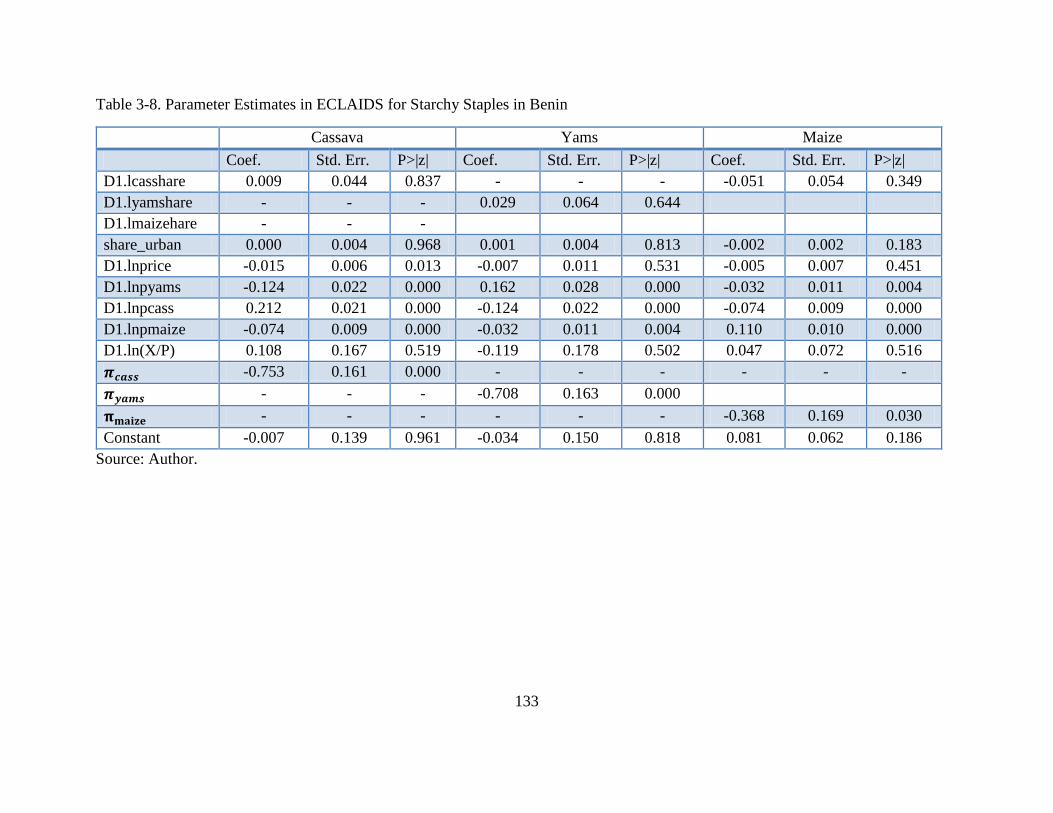
133
Table 3-8. Parameter Estimates in ECLAIDS for Starchy Staples in Benin
Cassava Yams Maize
Coef. Std. Err. P>|z| Coef. Std. Err. P>|z| Coef. Std. Err. P>|z|
D1.lcasshare 0.009 0.044 0.837 - - - -0.051 0.054 0.349
D1.lyamshare - - - 0.029 0.064 0.644
D1.lmaizehare - - -
share_urban 0.000 0.004 0.968 0.001 0.004 0.813 -0.002 0.002 0.183
D1.lnprice -0.015 0.006 0.013 -0.007 0.011 0.531 -0.005 0.007 0.451
D1.lnpyams -0.124 0.022 0.000 0.162 0.028 0.000 -0.032 0.011 0.004
D1.lnpcass 0.212 0.021 0.000 -0.124 0.022 0.000 -0.074 0.009 0.000
D1.lnpmaize -0.074 0.009 0.000 -0.032 0.011 0.004 0.110 0.010 0.000
D1.ln(X/P) 0.108 0.167 0.519 -0.119 0.178 0.502 0.047 0.072 0.516
𝝅𝒄𝒂𝒔𝒔 -0.753 0.161 0.000 - - - - - -
𝝅𝒚𝒂𝒎𝒔 - - - -0.708 0.163 0.000
𝛑𝐦𝐚𝐢𝐳𝐞 - - - - - - -0.368 0.169 0.030
Constant -0.007 0.139 0.961 -0.034 0.150 0.818 0.081 0.062 0.186
Source: Author.
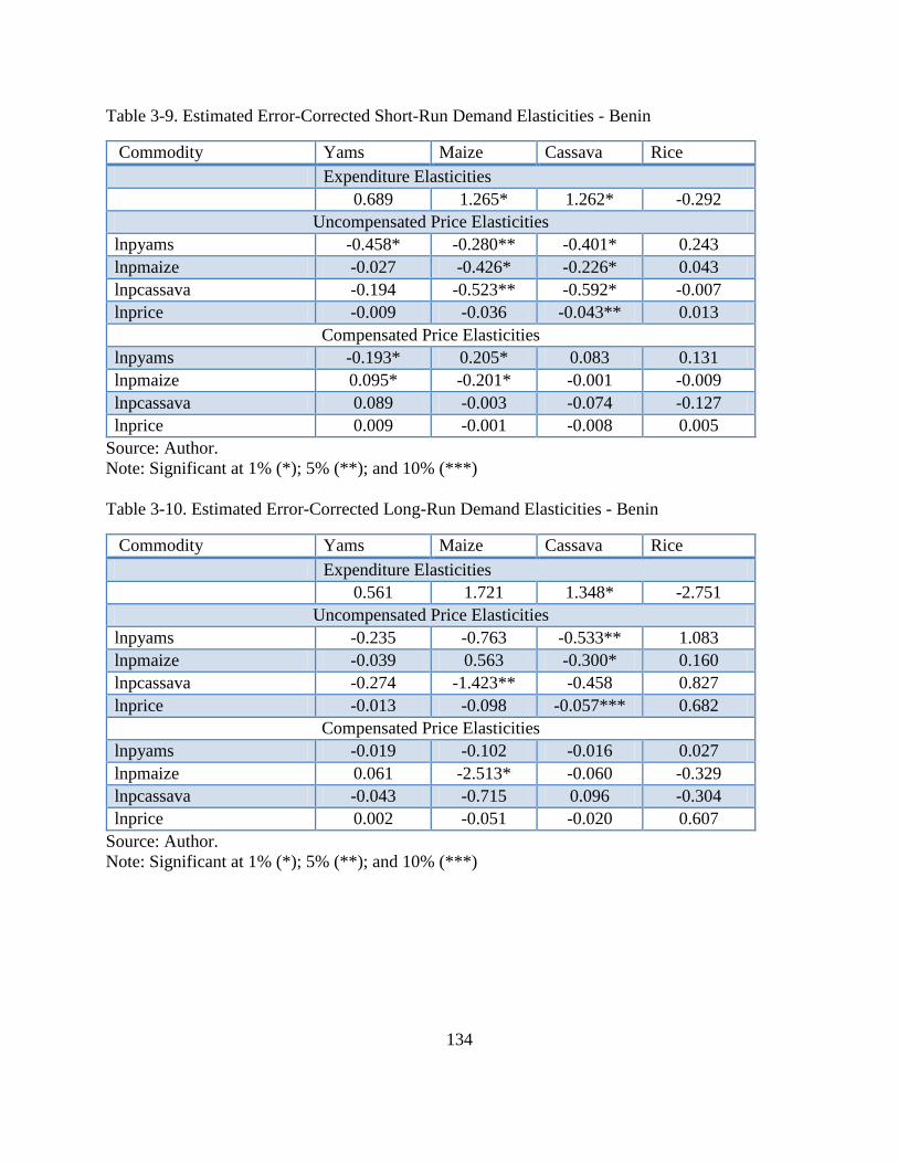
134
Table 3-9. Estimated Error-Corrected Short-Run Demand Elasticities - Benin
Commodity Yams Maize Cassava Rice
Expenditure Elasticities
0.689 1.265* 1.262* -0.292
Uncompensated Price Elasticities
lnpyams -0.458* -0.280** -0.401* 0.243
lnpmaize -0.027 -0.426* -0.226* 0.043
lnpcassava -0.194 -0.523** -0.592* -0.007
lnprice -0.009 -0.036 -0.043** 0.013
Compensated Price Elasticities
lnpyams -0.193* 0.205* 0.083 0.131
lnpmaize 0.095* -0.201* -0.001 -0.009
lnpcassava 0.089 -0.003 -0.074 -0.127
lnprice 0.009 -0.001 -0.008 0.005
Source: Author.
Note: Significant at 1% (*); 5% (**); and 10% (***)
Table 3-10. Estimated Error-Corrected Long-Run Demand Elasticities - Benin
Commodity Yams Maize Cassava Rice
Expenditure Elasticities
0.561 1.721 1.348* -2.751
Uncompensated Price Elasticities
lnpyams -0.235 -0.763 -0.533** 1.083
lnpmaize -0.039 0.563 -0.300* 0.160
lnpcassava -0.274 -1.423** -0.458 0.827
lnprice -0.013 -0.098 -0.057*** 0.682
Compensated Price Elasticities
lnpyams -0.019 -0.102 -0.016 0.027
lnpmaize 0.061 -2.513* -0.060 -0.329
lnpcassava -0.043 -0.715 0.096 -0.304
lnprice 0.002 -0.051 -0.020 0.607
Source: Author.
Note: Significant at 1% (*); 5% (**); and 10% (***)
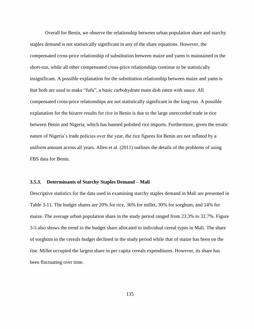
135
Overall for Benin, we observe the relationship between urban population share and starchy
staples demand is not statistically significant in any of the share equations. However, the
compensated cross-price relationship of substitution between maize and yams is maintained in the
short-run, while all other compensated cross-price relationships continue to be statistically
insignificant. A possible explanation for the substitution relationship between maize and yams is
that both are used to make “fufu”, a basic carbohydrate main dish eaten with sauce. All
compensated cross-price relationships are not statistically significant in the long-run. A possible
explanation for the bizarre results for rice in Benin is due to the large unrecorded trade in rice
between Benin and Nigeria, which has banned polished rice imports. Furthermore, given the erratic
nature of Nigeria’s trade policies over the year, the rice figures for Benin are not inflated by a
uniform amount across all years. Allen et al. (2011) outlines the details of the problems of using
FBS data for Benin.
3.5.3. Determinants of Starchy Staples Demand – Mali
Descriptive statistics for the data used in examining starchy staples demand in Mali are presented in
Table 3-11. The budget shares are 20% for rice, 36% for millet, 30% for sorghum, and 14% for
maize. The average urban population share in the study period ranged from 23.3% to 32.7%. Figure
3-5 also shows the trend in the budget share allocated to individual cereal types in Mali. The share
of sorghum in the cereals budget declined in the study period while that of maize has been on the
rise. Millet occupied the largest share in per capita cereals expenditures. However, its share has
been fluctuating over time.
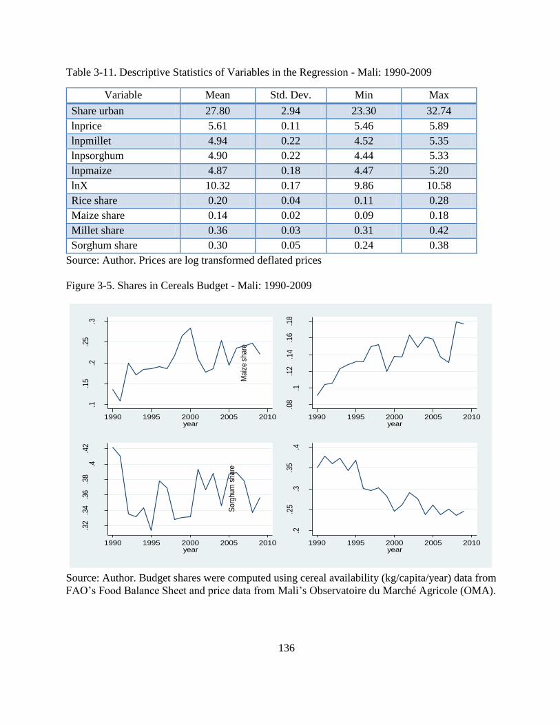
136
Table 3-11. Descriptive Statistics of Variables in the Regression - Mali: 1990-2009
Variable Mean Std. Dev. Min Max
Share urban 27.80 2.94 23.30 32.74
lnprice 5.61 0.11 5.46 5.89
lnpmillet 4.94 0.22 4.52 5.35
lnpsorghum 4.90 0.22 4.44 5.33
lnpmaize 4.87 0.18 4.47 5.20
lnX 10.32 0.17 9.86 10.58
Rice share 0.20 0.04 0.11 0.28
Maize share 0.14 0.02 0.09 0.18
Millet share 0.36 0.03 0.31 0.42
Sorghum share 0.30 0.05 0.24 0.38
Source: Author. Prices are log transformed deflated prices
Figure 3-5. Shares in Cereals Budget - Mali: 1990-2009
Source: Author. Budget shares were computed using cereal availability (kg/capita/year) data from
FAO’s Food Balance Sheet and price data from Mali’s Observatoire du Marché Agricole (OMA).
.1.1
5.2
.25
.3
Ric
e s
hare
1990 1995 2000 2005 2010year
.08
.1.1
2.1
4.1
6.1
8
Maiz
e s
hare
1990 1995 2000 2005 2010year
.32
.34
.36
.38
.4.4
2
Mill
et sh
are
1990 1995 2000 2005 2010year
.2.2
5.3
.35
.4
Sorg
hum
share
1990 1995 2000 2005 2010year
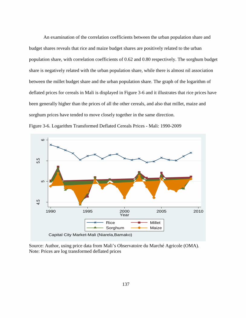
137
An examination of the correlation coefficients between the urban population share and
budget shares reveals that rice and maize budget shares are positively related to the urban
population share, with correlation coefficients of 0.62 and 0.80 respectively. The sorghum budget
share is negatively related with the urban population share, while there is almost nil association
between the millet budget share and the urban population share. The graph of the logarithm of
deflated prices for cereals in Mali is displayed in Figure 3-6 and it illustrates that rice prices have
been generally higher than the prices of all the other cereals, and also that millet, maize and
sorghum prices have tended to move closely together in the same direction.
Figure 3-6. Logarithm Transformed Deflated Cereals Prices - Mali: 1990-2009
Source: Author, using price data from Mali’s Observatoire du Marché Agricole (OMA).
Note: Prices are log transformed deflated prices
4.5
55
.56
Log
arith
m o
f De
flate
d P
rice
s
1990 1995 2000 2005 2010Year
Rice Millet
Sorghum Maize
Capital City Market-Mali (Niarela,Bamako)
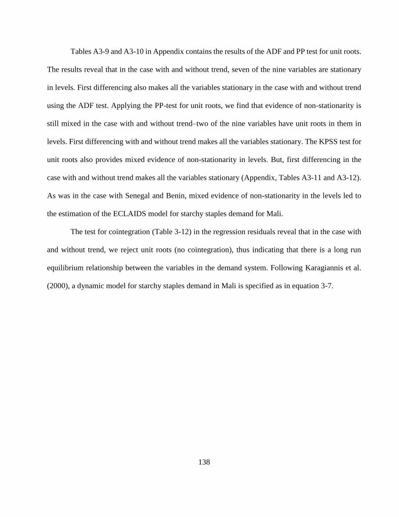
138
Tables A3-9 and A3-10 in Appendix contains the results of the ADF and PP test for unit roots.
The results reveal that in the case with and without trend, seven of the nine variables are stationary
in levels. First differencing also makes all the variables stationary in the case with and without trend
using the ADF test. Applying the PP-test for unit roots, we find that evidence of non-stationarity is
still mixed in the case with and without trend–two of the nine variables have unit roots in them in
levels. First differencing with and without trend makes all the variables stationary. The KPSS test for
unit roots also provides mixed evidence of non-stationarity in levels. But, first differencing in the
case with and without trend makes all the variables stationary (Appendix, Tables A3-11 and A3-12).
As was in the case with Senegal and Benin, mixed evidence of non-stationarity in the levels led to
the estimation of the ECLAIDS model for starchy staples demand for Mali.
The test for cointegration (Table 3-12) in the regression residuals reveal that in the case with
and without trend, we reject unit roots (no cointegration), thus indicating that there is a long run
equilibrium relationship between the variables in the demand system. Following Karagiannis et al.
(2000), a dynamic model for starchy staples demand in Mali is specified as in equation 3-7.
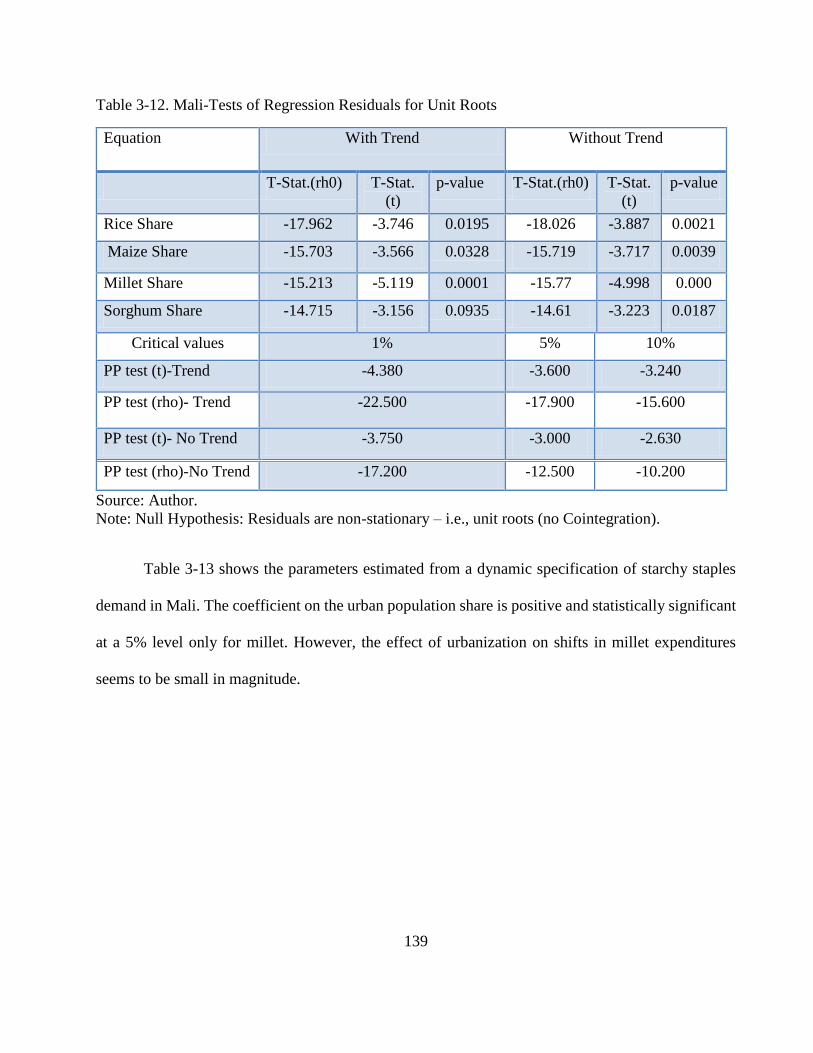
139
Table 3-12. Mali-Tests of Regression Residuals for Unit Roots
Equation With Trend Without Trend
T-Stat.(rh0) T-Stat.
(t)
p-value T-Stat.(rh0) T-Stat.
(t)
p-value
Rice Share -17.962 -3.746 0.0195 -18.026 -3.887 0.0021
Maize Share -15.703 -3.566 0.0328 -15.719 -3.717 0.0039
Millet Share -15.213 -5.119 0.0001 -15.77 -4.998 0.000
Sorghum Share -14.715 -3.156 0.0935 -14.61 -3.223 0.0187
Critical values 1% 5% 10%
PP test (t)-Trend -4.380 -3.600 -3.240
PP test (rho)- Trend -22.500 -17.900 -15.600
PP test (t)- No Trend -3.750 -3.000 -2.630
PP test (rho)-No Trend -17.200 -12.500 -10.200
Source: Author.
Note: Null Hypothesis: Residuals are non-stationary – i.e., unit roots (no Cointegration).
Table 3-13 shows the parameters estimated from a dynamic specification of starchy staples
demand in Mali. The coefficient on the urban population share is positive and statistically significant
at a 5% level only for millet. However, the effect of urbanization on shifts in millet expenditures
seems to be small in magnitude.
140
Table 3-13. Parameter Estimates from Error-Corrected Linear AIDS model - Mali
Rice Share Millet Sorghum
Variables Coef. Std. Err. P>|z| Coef. Std. Err. P>|z| Coef. Std. Err. P>|z|
D1.lriceshare 0.307 0.062 0.000
D1.lmilshare 0.248 0.085 0.004
D1.lsorgshare 0.520 0.098 0.000
share_urban 0.000 0.002 0.879 0.002 0.001 0.023 -0.002 0.002 0.482
D1.lnprice 0.045 0.058 0.437 -0.147 0.034 0.000 0.051 0.039 0.192
D1.lnpmil -0.147 0.034 0.000 0.277 0.041 0.000 -0.065 0.033 0.047
D1.lnpmaize 0.008 0.033 0.803 -0.127 0.023 0.000 0.066 0.030 0.025
D1.lnpsorg 0.051 0.039 0.192 -0.065 0.033 0.047 0.007 0.032 0.824
Dln(X/P) -0.491 0.165 0.003 0.159 0.085 0.062 0.235 0.171 0.169
𝝅𝒓𝒊𝒄𝒆 -1.476 0.175 0.000 - - - - - -
𝝅𝒎𝒊𝒍𝒍𝒆𝒕 - - - -1.257 0.174 0.000 - - -
𝝅𝒔𝒐𝒓𝒈𝒉𝒖𝒎 - - - - - - -1.580 0.159 0.000
Constant -0.001 0.061 0.991 -0.070 0.030 0.018 0.039 0.062 0.535
Source: Author.
141
The relationship between urban population share and rice and sorghum are not statistically
significant. The lagged residuals from the cointegrating regressions are negative in all three share
equations but only statistically significant in the rice and millet share equations. Per capita starchy
staples expenditures are also statistically significant in the rice share equation and in the millet
equation.
Tables 3-14 and 3-15 show the estimated short-run and long-run elasticities from the
starchy staples demand model for Mali. The short-run expenditure elasticities are statistically
significant at a 1% level and also greater than unity for millet, sorghum and maize, indicating these
cereals are expenditure elastic. The same story is preserved in the long-run (Table 3-15). All the
own-price uncompensated price elasticities exhibit the expected negative sign and are statistically
significant in the short-run and in the long-run. Rice, sorghum, and maize also exhibit a downward
sloping compensated demand curve in the short-run and long-run. The short-run compensated
cross-price elasticities reveal that maize is a substitute for rice and sorghum, rice is a substitute for
sorghum, and maize is a complement to millet. In the long-run all compensated cross-price
relationships are that of substitution, with the exception of maize and millet that are complements,
and millet and sorghum, and rice and millet with no statistically significant long-run relationship.
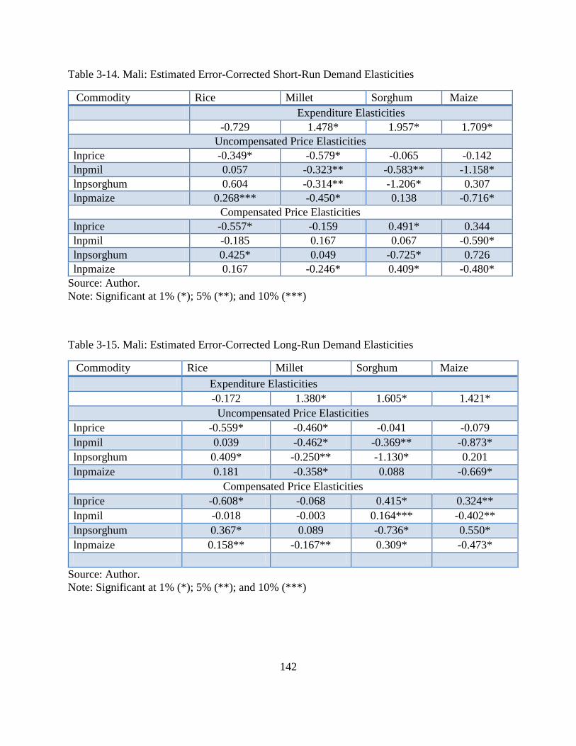
142
Table 3-14. Mali: Estimated Error-Corrected Short-Run Demand Elasticities
Commodity Rice Millet Sorghum Maize
Expenditure Elasticities
-0.729 1.478* 1.957* 1.709*
Uncompensated Price Elasticities
lnprice -0.349* -0.579* -0.065 -0.142
lnpmil 0.057 -0.323** -0.583** -1.158*
lnpsorghum 0.604 -0.314** -1.206* 0.307
lnpmaize 0.268*** -0.450* 0.138 -0.716*
Compensated Price Elasticities
lnprice -0.557* -0.159 0.491* 0.344
lnpmil -0.185 0.167 0.067 -0.590*
lnpsorghum 0.425* 0.049 -0.725* 0.726
lnpmaize 0.167 -0.246* 0.409* -0.480*
Source: Author.
Note: Significant at 1% (*); 5% (**); and 10% (***)
Table 3-15. Mali: Estimated Error-Corrected Long-Run Demand Elasticities
Commodity Rice Millet Sorghum Maize
Expenditure Elasticities
-0.172 1.380* 1.605* 1.421*
Uncompensated Price Elasticities
lnprice -0.559* -0.460* -0.041 -0.079
lnpmil 0.039 -0.462* -0.369** -0.873*
lnpsorghum 0.409* -0.250** -1.130* 0.201
lnpmaize 0.181 -0.358* 0.088 -0.669*
Compensated Price Elasticities
lnprice -0.608* -0.068 0.415* 0.324**
lnpmil -0.018 -0.003 0.164*** -0.402**
lnpsorghum 0.367* 0.089 -0.736* 0.550*
lnpmaize 0.158** -0.167** 0.309* -0.473*
Source: Author.
Note: Significant at 1% (*); 5% (**); and 10% (***)
143
3.6. Chapter Summary
The main objective of the preceding analysis was to examine the aggregate-level determinants of
starchy staples demand in Benin, Mali and Senegal. An Error Corrected linearized Almost Ideal
demand system (ECLAIDS) was specified following the results of the test for the stochastic
properties of the data (unit roots and cointegration). A specific goal of the analysis was to
determine any statistical association between the growth in urban population share and the
demand for traditional coarse grains such as millet and sorghum. Although domestic price trends
are not strictly uniform across all three countries, on the whole similar trends could be observed
in all three countries for rice prices relative to coarse grains. Common to Mali and Senegal in the
Sahel region of WA is an increasing trend in the share of maize and rice and a declining trend in
the share of millet and sorghum in the starchy staples budget over time. In Benin, the shares of
individual starchy staple types in the starchy staple budget in the period 1990-2009 have been
fluctuating, not exhibiting any noticeable trend.
The analysis of cereals demand after correcting for the unit root properties of the data
does not provide any support for a statistical association between the urban population share and
cereals consumption behavior in Senegal, but points to a statistically significant, but small,
relationship between millet and urban population share in Mali. A principal channel31 through
which urbanization affects consumption is by increasing per capita incomes. By including per
capita expenditures on starchy staples as a separate variable in the estimated model, the model
specification already controls for per capita expenditure. However, while the coefficient of
urbanization and per capita expenditures picks up the individual effects of each of these
31 Other channels include changes in lifestyle, for instance increased female employment outside their homes.
144
variables, both variables could interact to generate additional effects on consumption. The
insignificance of the urbanization variable in the dynamic specification could be the result of the
way in which the variable is introduced into the model. Ideally, one would like to add an
interaction term between the urban population share and starchy staples expenditures. However,
due to the small number of observations, additional terms will pose degrees of freedom
problems, making it impossible to estimate the model. The manner in which the urban population
share is incorporated in this study is therefore the most straightforward given starchy staples
price data limitations.
As discussed in Chapter 1, evidence on the role of relative cereals prices in influencing
cereals consumption in West Africa has been mixed. It has been argued that changes in rice
consumption, for instance, are more linked to structural factors like urbanization and to a lesser
extent short-term price changes. The Hicksian cross-price elasticities from the error-corrected
demand model provide evidence of a statistically significant relationship of substitution in the
short-run and long-run between rice and sorghum as hypothesized for Mali and Senegal. While
in Senegal, rice is found to be a complement to millet in both the short-run and in the long-run,
in Mali, rice and millet are substitutes but the relationship is not statistically significant.
Furthermore, in Senegal and Mali the relationship between rice and maize is positive but not
statistically significant in the short-run. However, while the latter relationship continues to be
insignificant in the Senegal in the long-run, in Mali, rice and maize have a statistically significant
relationship of substitution in the long-run. The dynamic specification (long-run and short-run)
for Senegal provides evidence of substitution of maize for sorghum and complementarity
between maize and millet. The results also reveal that in spite of the negative association
between urbanization and coarse grains (millet and sorghum) shares as shown by the correlation
145
coefficients, the expenditure elasticities are more elastic for millet and sorghum than they are for
rice in Senegal and Mali. This finding is contrary to the expectation that traditional coarse grains
are expenditure inelastic and warrants more investigation of starchy staples consumption
behavior by place of residence within the same income group.
Overall for Benin, we observe that most compensated cross-price relationships are not
statistically significant in both the short-run and long-run. A possible explanation for the bizarre
results for rice in Benin is the large unrecorded trade in rice between Benin and Nigeria, which
has banned polished rice imports. This unrecorded trade may make the FBS per capita rice
availability figures for Benin unreliable indicators of the true consumption levels.
A limitation of the aggregate results is that they do not sufficiently capture the effects of
structural change on consumption coming from changes in non-price factors, such as income
distribution. Such estimations implicitly assume that many other factors remain constant. Even
more, in most cases the national averages hide contrasting sub-national realities. The distribution
of income at the sub-national or micro level is probably a more critical determinant of starchy
staples consumption than is the level of aggregate national per capita expenditures. Another big
limitation is the intra-annual aggregation that takes place when one uses annual data—e.g.,
annual price data. Delgado and Reardon (1991) argue that although aggregate results are still
very useful for looking at long-term consumption trends, the diagnosis of what is really pushing
consumption behavior requires micro-level work that takes into account the relevant non-price
factors. Chapter 4 examines the micro-level factors that influence cereals consumption in Mali
using Mali’s 2006 household budget survey data. This allows us to explore further the
discrepancies found in different regions of Mali and across households of different social and
economic characteristics.

146
APPENDIX
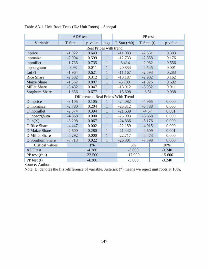
147
Table A3-1. Unit Root Tests (H0: Unit Roots) – Senegal
ADF test PP test
Variable T-Stat. p-value lags T-Stat.(rh0) T-Stat. (t) p-value
Real Prices with trend
lnprice -1.922 0.643 1 -11.083 -2.551 0.303
lnpmaize -2.004 0.599 1 -12.733 -2.858 0.176
lnpmillet -1.735 0.735 1 -8.414 -2.082 0.556
lnpsorghum -3.93 0.011 1 -20.834 -4.545 0.001
Ln(P) -1.964 0.621 1 -11.167 -2.593 0.283
Rice Share -2.532 0.312 1 -13.187 -2.902 0.162
Maize Share -1.562 0.807 1 -5.789 -1.826 0.692
Millet Share -3.432 0.047 1 -18.012 -3.932 0.011
Sorghum Share -1.856 0.677 1 -15.608 -3.51 0.038
Differenced Real Prices With Trend
D.lnprice -3.105 0.105 1 -24.082 -4.965 0.000
D.lnpmaize -2.780 0.204 1 -25.312 -5.788 0.000
D.lnpmillet -2.374 0.394 1 -21.639 -4.57 0.001
D.lnpsorghum -4.868 0.000 1 -25.003 -6.668 0.000
D.ln(X) -3.298 0.067 1 -24.836 -5.176 0.000
D.Rice Share -4.447 0.002 1 -22.159 -4.915 0.000
D.Maize Share -2.600 0.280 1 -21.442 -4.609 0.001
D.Millet Share -5.292 0.000 1 -22.717 -5.473 0.000
D.Sorghum Share -3.713 0.022 1 -26.801 -7.398 0.000
Critical values 1% 5% 10%
ADF test -4.380 -3.600 -3.240
PP test (rho) -22.500 -17.900 -15.600
PP test (t) -4.380 -3.600 -3.240 Source: Author.
Note: D. denotes the first-difference of variable. Asterisk (*) means we reject unit roots at 10%.
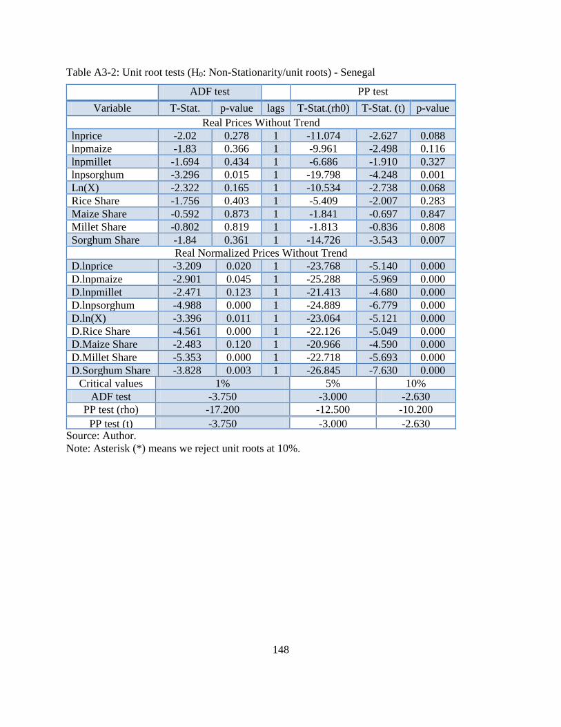
148
Table A3-2: Unit root tests (H0: Non-Stationarity/unit roots) - Senegal
ADF test PP test
Variable T-Stat. p-value lags T-Stat.(rh0) T-Stat. (t) p-value
Real Prices Without Trend
lnprice -2.02 0.278 1 -11.074 -2.627 0.088
lnpmaize -1.83 0.366 1 -9.961 -2.498 0.116
lnpmillet -1.694 0.434 1 -6.686 -1.910 0.327
lnpsorghum -3.296 0.015 1 -19.798 -4.248 0.001
Ln(X) -2.322 0.165 1 -10.534 -2.738 0.068
Rice Share -1.756 0.403 1 -5.409 -2.007 0.283
Maize Share -0.592 0.873 1 -1.841 -0.697 0.847
Millet Share -0.802 0.819 1 -1.813 -0.836 0.808
Sorghum Share -1.84 0.361 1 -14.726 -3.543 0.007
Real Normalized Prices Without Trend
D.lnprice -3.209 0.020 1 -23.768 -5.140 0.000
D.lnpmaize -2.901 0.045 1 -25.288 -5.969 0.000
D.lnpmillet -2.471 0.123 1 -21.413 -4.680 0.000
D.lnpsorghum -4.988 0.000 1 -24.889 -6.779 0.000
D.ln(X) -3.396 0.011 1 -23.064 -5.121 0.000
D.Rice Share -4.561 0.000 1 -22.126 -5.049 0.000
D.Maize Share -2.483 0.120 1 -20.966 -4.590 0.000
D.Millet Share -5.353 0.000 1 -22.718 -5.693 0.000
D.Sorghum Share -3.828 0.003 1 -26.845 -7.630 0.000
Critical values 1% 5% 10%
ADF test -3.750 -3.000 -2.630
PP test (rho) -17.200 -12.500 -10.200
PP test (t) -3.750 -3.000 -2.630 Source: Author.
Note: Asterisk (*) means we reject unit roots at 10%.
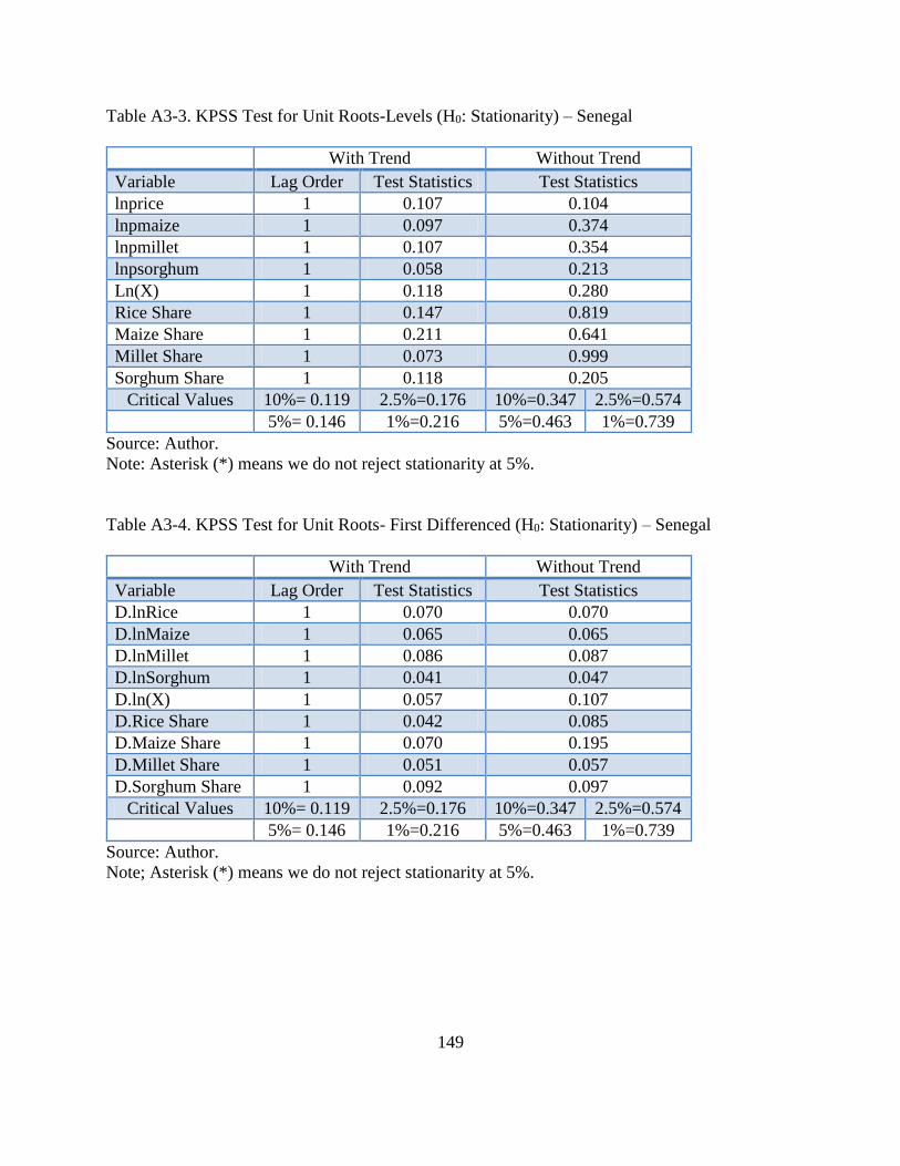
149
Table A3-3. KPSS Test for Unit Roots-Levels (H0: Stationarity) – Senegal
With Trend Without Trend
Variable Lag Order Test Statistics Test Statistics
lnprice 1 0.107 0.104
lnpmaize 1 0.097 0.374
lnpmillet 1 0.107 0.354
lnpsorghum 1 0.058 0.213
Ln(X) 1 0.118 0.280
Rice Share 1 0.147 0.819
Maize Share 1 0.211 0.641
Millet Share 1 0.073 0.999
Sorghum Share 1 0.118 0.205
Critical Values 10%= 0.119 2.5%=0.176 10%=0.347 2.5%=0.574
5%= 0.146 1%=0.216 5%=0.463 1%=0.739
Source: Author.
Note: Asterisk (*) means we do not reject stationarity at 5%.
Table A3-4. KPSS Test for Unit Roots- First Differenced (H0: Stationarity) – Senegal
With Trend Without Trend
Variable Lag Order Test Statistics Test Statistics
D.lnRice 1 0.070 0.070
D.lnMaize 1 0.065 0.065
D.lnMillet 1 0.086 0.087
D.lnSorghum 1 0.041 0.047
D.ln(X) 1 0.057 0.107
D.Rice Share 1 0.042 0.085
D.Maize Share 1 0.070 0.195
D.Millet Share 1 0.051 0.057
D.Sorghum Share 1 0.092 0.097
Critical Values 10%= 0.119 2.5%=0.176 10%=0.347 2.5%=0.574
5%= 0.146 1%=0.216 5%=0.463 1%=0.739
Source: Author.
Note; Asterisk (*) means we do not reject stationarity at 5%.
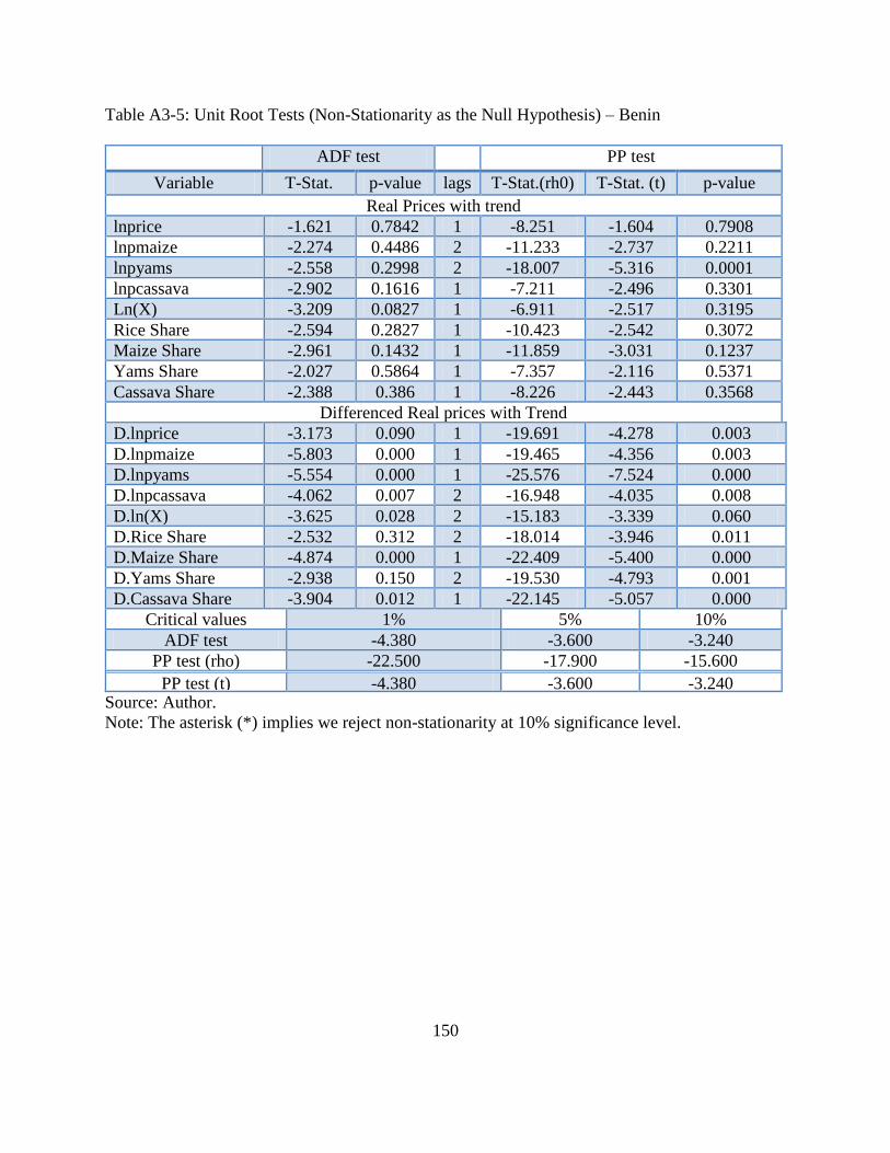
150
Table A3-5: Unit Root Tests (Non-Stationarity as the Null Hypothesis) – Benin
ADF test PP test
Variable T-Stat. p-value lags T-Stat.(rh0) T-Stat. (t) p-value
Real Prices with trend
lnprice -1.621 0.7842 1 -8.251 -1.604 0.7908
lnpmaize -2.274 0.4486 2 -11.233 -2.737 0.2211
lnpyams -2.558 0.2998 2 -18.007 -5.316 0.0001
lnpcassava -2.902 0.1616 1 -7.211 -2.496 0.3301
Ln(X) -3.209 0.0827 1 -6.911 -2.517 0.3195
Rice Share -2.594 0.2827 1 -10.423 -2.542 0.3072
Maize Share -2.961 0.1432 1 -11.859 -3.031 0.1237
Yams Share -2.027 0.5864 1 -7.357 -2.116 0.5371
Cassava Share -2.388 0.386 1 -8.226 -2.443 0.3568
Differenced Real prices with Trend
D.lnprice -3.173 0.090 1 -19.691 -4.278 0.003
D.lnpmaize -5.803 0.000 1 -19.465 -4.356 0.003
D.lnpyams -5.554 0.000 1 -25.576 -7.524 0.000
D.lnpcassava -4.062 0.007 2 -16.948 -4.035 0.008
D.ln(X) -3.625 0.028 2 -15.183 -3.339 0.060
D.Rice Share -2.532 0.312 2 -18.014 -3.946 0.011
D.Maize Share -4.874 0.000 1 -22.409 -5.400 0.000
D.Yams Share -2.938 0.150 2 -19.530 -4.793 0.001
D.Cassava Share -3.904 0.012 1 -22.145 -5.057 0.000
Critical values 1% 5% 10%
ADF test -4.380 -3.600 -3.240
PP test (rho) -22.500 -17.900 -15.600
PP test (t) -4.380 -3.600 -3.240 Source: Author.
Note: The asterisk (*) implies we reject non-stationarity at 10% significance level.
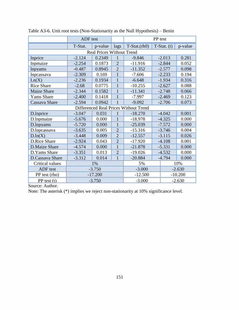
151
Table A3-6. Unit root tests (Non-Stationarity as the Null Hypothesis) – Benin
ADF test PP test
T-Stat. p-value lags T-Stat.(rh0) T-Stat. (t) p-value
Real Prices Without Trend
lnprice -2.124 0.2349 1 -9.846 -2.013 0.281
lnpmaize -2.254 0.1873 2 -11.916 -2.844 0.052
lnpyams -0.487 0.8945 2 -11.352 -2.577 0.098
lnpcassava -2.309 0.169 1 -7.606 -2.233 0.194
Ln(X) -2.236 0.1934 1 -6.648 -1.934 0.316
Rice Share -2.68 0.0775 1 -10.255 -2.627 0.088
Maize Share -2.344 0.1582 1 -11.341 -2.748 0.066
Yams Share -2.400 0.1418 1 -7.997 -2.469 0.123
Cassava Share -2.594 0.0942 1 -9.092 -2.706 0.073
Differenced Real Prices Without Trend
D.lnprice -3.047 0.031 1 -18.270 -4.042 0.001
D.lnpmaize -5.676 0.000 1 -18.978 -4.325 0.000
D.lnpyams -5.720 0.000 1 -25.039 -7.572 0.000
D.lnpcassava -3.635 0.005 2 -15.316 -3.746 0.004
D.ln(X) -3.448 0.009 2 -12.557 -3.115 0.026
D.Rice Share -2.924 0.043 2 -17.920 -4.108 0.001
D.Maize Share -4.574 0.000 1 -21.878 -5.331 0.000
D.Yams Share -3.351 0.013 2 -19.026 -4.532 0.000
D.Cassava Share -3.312 0.014 1 -20.884 -4.794 0.000
Critical values 1% 5% 10%
ADF test -3.750 -3.000 -2.630
PP test (rho) -17.200 -12.500 -10.200
PP test (t) -3.750 -3.000 -2.630 Source: Author.
Note: The asterisk (*) implies we reject non-stationarity at 10% significance level.
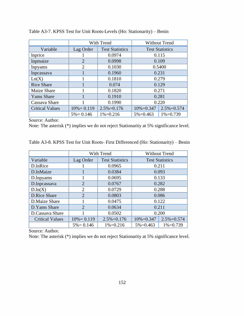
152
Table A3-7. KPSS Test for Unit Roots-Levels (Ho: Stationarity) – Benin
With Trend Without Trend
Variable Lag Order Test Statistics Test Statistics
lnprice 1 0.0974 0.115
lnpmaize 2 0.0998 0.109
lnpyams 2 0.1030 0.5400
lnpcassava 1 0.1960 0.231
Ln(X) 1 0.1810 0.279
Rice Share 1 0.074 0.129
Maize Share 1 0.1820 0.271
Yams Share 1 0.1910 0.281
Cassava Share 1 0.1990 0.220
Critical Values 10%= 0.119 2.5%=0.176 10%=0.347 2.5%=0.574
5%= 0.146 1%=0.216 5%=0.463 1%=0.739
Source: Author.
Note: The asterisk (*) implies we do not reject Stationarity at 5% significance level.
Table A3-8. KPSS Test for Unit Roots- First Differenced (Ho: Stationarity) – Benin
With Trend Without Trend
Variable Lag Order Test Statistics Test Statistics
D.lnRice 1 0.0965 0.211
D.lnMaize 1 0.0384 0.093
D.lnpyams 1 0.0695 0.133
D.lnpcassava 2 0.0767 0.282
D.ln(X) 2 0.0729 0.288
D.Rice Share 2 0.0803 0.086
D.Maize Share 1 0.0475 0.122
D.Yams Share 2 0.0634 0.211
D.Cassava Share 1 0.0502 0.200
Critical Values 10%= 0.119 2.5%=0.176 10%=0.347 2.5%=0.574
5%= 0.146 1%=0.216 5%=0.463 1%=0.739
Source: Author.
Note: The asterisk (*) implies we do not reject Stationarity at 5% significance level.
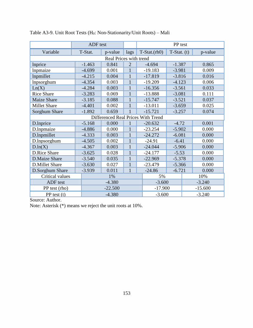
153
Table A3-9. Unit Root Tests (H0: Non-Stationarity/Unit Roots) – Mali
ADF test PP test
Variable T-Stat. p-value lags T-Stat.(rh0) T-Stat. (t) p-value
Real Prices with trend
lnprice -1.463 0.841 2 -4.694 -1.387 0.865
lnpmaize -4.699 0.001 1 -19.183 -3.981 0.009
lnpmillet -4.215 0.004 1 -17.819 -3.816 0.016
lnpsorghum -4.354 0.003 1 -19.209 -4.123 0.006
Ln(X) -4.284 0.003 1 -16.356 -3.561 0.033
Rice Share -3.283 0.069 1 -13.888 -3.081 0.111
Maize Share -3.185 0.088 1 -15.747 -3.521 0.037
Millet Share -4.401 0.002 1 -13.011 -3.659 0.025
Sorghum Share -1.892 0.659 1 -15.721 -3.257 0.074
Differenced Real Prices With Trend
D.lnprice -5.168 0.000 1 -20.632 -4.72 0.001
D.lnpmaize -4.886 0.000 1 -23.254 -5.902 0.000
D.lnpmillet -4.333 0.003 1 -24.272 -6.081 0.000
D.lnpsorghum -4.505 0.002 1 -24.91 -6.41 0.000
D.ln(X) -4.367 0.003 1 -24.044 -5.906 0.000
D.Rice Share -3.625 0.028 1 -24.177 -5.53 0.000
D.Maize Share -3.540 0.035 1 -22.969 -5.378 0.000
D.Millet Share -3.630 0.027 1 -23.479 -5.366 0.000
D.Sorghum Share -3.939 0.011 1 -24.86 -6.721 0.000
Critical values 1% 5% 10%
ADF test -4.380 -3.600 -3.240
PP test (rho) -22.500 -17.900 -15.600
PP test (t) -4.380 -3.600 -3.240 Source: Author.
Note: Asterisk (*) means we reject the unit roots at 10%.
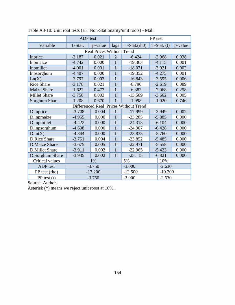
154
Table A3-10: Unit root tests (H0: Non-Stationarity/unit roots) - Mali
ADF test PP test
Variable T-Stat. p-value lags T-Stat.(rh0) T-Stat. (t) p-value
Real Prices Without Trend
lnprice -3.187 0.021 2 -6.424 -2.968 0.038
lnpmaize -4.742 0.000 1 -19.363 -4.115 0.001
lnpmillet -4.001 0.001 1 -18.071 -3.921 0.002
lnpsorghum -4.407 0.000 1 -19.352 -4.275 0.001
Ln(X) -3.797 0.003 1 -16.843 -3.595 0.006
Rice Share -3.178 0.021 1 -8.790 -2.619 0.089
Maize Share -1.622 0.472 1 -6.382 -2.068 0.258
Millet Share -3.758 0.003 1 -13.509 -3.662 0.005
Sorghum Share -1.208 0.670 1 -1.998 -1.020 0.746
Differenced Real Prices Without Trend
D.lnprice -3.708 0.004 1 -17.999 -3.949 0.002
D.lnpmaize -4.955 0.000 1 -23.285 -5.885 0.000
D.lnpmillet -4.422 0.000 1 -24.313 -6.104 0.000
D.lnpsorghum -4.608 0.000 1 -24.907 -6.428 0.000
D.ln(X) -4.344 0.000 1 -23.835 -5.760 0.000
D.Rice Share -3.751 0.004 1 -23.852 -5.485 0.000
D.Maize Share -3.675 0.005 1 -22.971 -5.558 0.000
D.Millet Share -3.911 0.002 1 -22.965 -5.423 0.000
D.Sorghum Share -3.935 0.002 1 -25.115 -6.821 0.000
Critical values 1% 5% 10%
ADF test -3.750 -3.000 -2.630
PP test (rho) -17.200 -12.500 -10.200
PP test (t) -3.750 -3.000 -2.630 Source: Author.
Asterisk (*) means we reject unit roost at 10%.
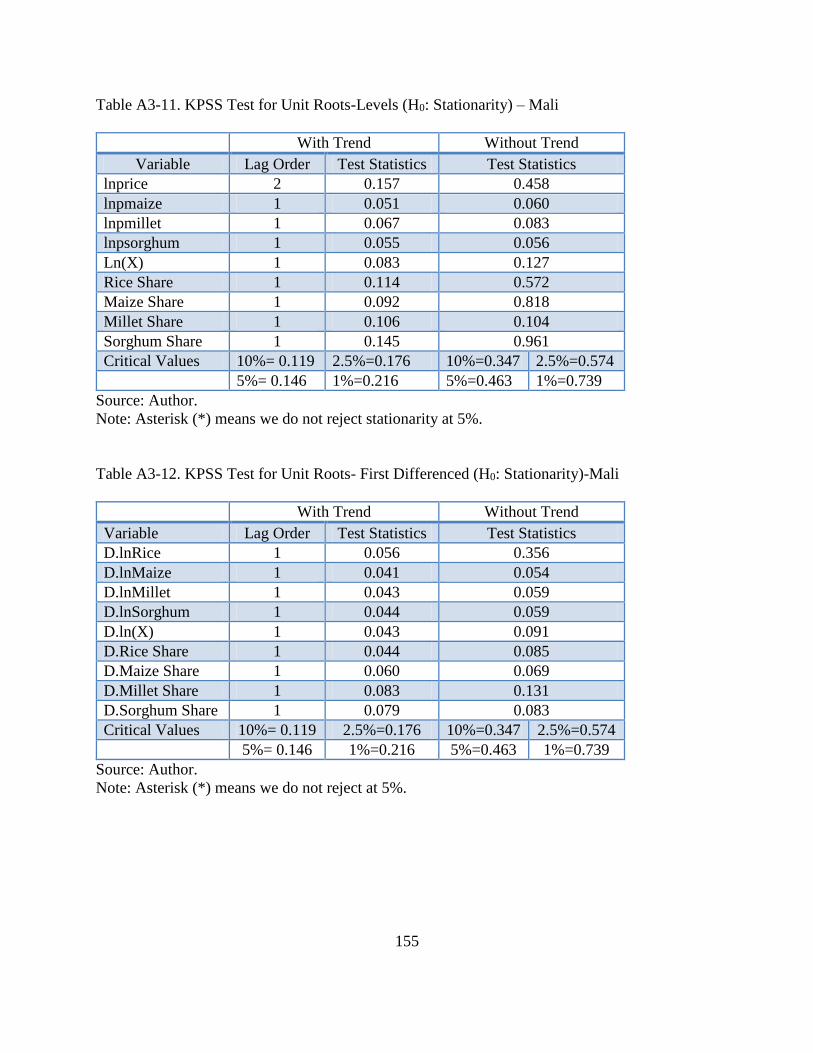
155
Table A3-11. KPSS Test for Unit Roots-Levels (H0: Stationarity) – Mali
With Trend Without Trend
Variable Lag Order Test Statistics Test Statistics
lnprice 2 0.157 0.458
lnpmaize 1 0.051 0.060
lnpmillet 1 0.067 0.083
lnpsorghum 1 0.055 0.056
Ln(X) 1 0.083 0.127
Rice Share 1 0.114 0.572
Maize Share 1 0.092 0.818
Millet Share 1 0.106 0.104
Sorghum Share 1 0.145 0.961
Critical Values 10%= 0.119 2.5%=0.176 10%=0.347 2.5%=0.574
5%= 0.146 1%=0.216 5%=0.463 1%=0.739
Source: Author.
Note: Asterisk (*) means we do not reject stationarity at 5%.
Table A3-12. KPSS Test for Unit Roots- First Differenced (H0: Stationarity)-Mali
With Trend Without Trend
Variable Lag Order Test Statistics Test Statistics
D.lnRice 1 0.056 0.356
D.lnMaize 1 0.041 0.054
D.lnMillet 1 0.043 0.059
D.lnSorghum 1 0.044 0.059
D.ln(X) 1 0.043 0.091
D.Rice Share 1 0.044 0.085
D.Maize Share 1 0.060 0.069
D.Millet Share 1 0.083 0.131
D.Sorghum Share 1 0.079 0.083
Critical Values 10%= 0.119 2.5%=0.176 10%=0.347 2.5%=0.574
5%= 0.146 1%=0.216 5%=0.463 1%=0.739
Source: Author.
Note: Asterisk (*) means we do not reject at 5%.
156
CHAPTER 4. HOUSEHOLD-LEVEL EVIDENCE OF CEREALS DEMAND IN
URBAN AND RURAL MALI
4.1. Background and Problem Statement
The aggregate, country-level analysis of food demand based on FBS data from Chapter 3 is a
good starting point for understanding major drivers of the demand for starchy staples in West
Africa. However, the information it provides permits only the identification of the general
priorities for consumption analysis and overall food policy attention. The limitations of the FBS
are quite well known: a) its failure to disaggregate supply by income class and b) its failure to
provide information on the distribution of food availability geographically within a country. As a
result, an analysis thereof ignores the effects of the distribution of income and of differences in
food supply across regions on food demand. Such a disaggregation is essential in bringing the
food situation into clearer focus. Even more, several factors at the household-level work to
determine food demand behavior, and these need to be understood in order to design effective
food policies.
This chapter aims to provide micro-level evidence on food demand in Mali by means of a
household-level disaggregated, multivariate analysis using household budget survey (HBS) data.
An analysis of food demand disaggregated at the household level helps to identify households
that are most vulnerable to inadequate food intake and their geographic location; and in
particular in understanding the behavioral parameters underlying any adjustment to the economic
environment. A multivariate analysis that is grounded in economic theory provides estimates of
microeconomic measures of households’ consumption responsiveness to changes in the amount
of resources available for consumption and also allows us to test the responsiveness of demand
to other arguments included in the demand function (e.g., prices). Estimation at the household
157
level allows not only the incorporation of household consumption variables (economic and
socio-demographic) into the analysis, but even more important, the interest of this type of
analysis lies in the estimation of price and income elasticities of demand which: a) take into
account differences in the distribution of income across households and b) capture the extent to
which price differences resulting from differences in food supply conditions as well as
differences in tastes and preferences across regions influence food demand. Such information is
needed for a much precise description of food security problems, in designing programs that
target food assistance efficiently and in evaluating the effect of various policies and other
targeted programs to alleviate food insecurity.
4.2. Research Questions and Hypotheses
The main objective of this chapter is to analyze HBS data for Mali in order to estimate
consumption parameters. Separate food demand estimates will be provided by place of residence
(urban/rural) and by per capita income groups. Specifically, the analysis asks the following
questions:
What factors influence the demand for individual cereals and the substitution among
individual cereal types?
How does food consumption behavior differ across households of different income levels?
How does the structure of food demand differ by place of residence (rural/urban)?
The following hypotheses will be tested:
Hypothesis 4.1: Cereals expenditure elasticities are higher for poorer than for richer households.
Engel’s law also predicts that the proportion of income spent on food declines with income. We
therefore expect expenditure elasticities to be higher for lower income groups.
158
Hypothesis 4.2: Rice demand is less responsive (inelastic) to price changes (relative to coarse
grains) in urban areas than in rural areas. Due to the high opportunity cost of time and
convenience in the urban area, one would expect urban households to prefer rice to coarse grains
and therefore be less sensitive to changes in rice prices.
Hypothesis 4.3: The Marshallian own-price elasticities of cereals demand are more elastic
(larger in absolute terms) for lower income households than higher income households. For
poorer households spending a higher percentage of their income on food (Engel’s law) the
income effect of a change in the price of food is expected to be substantial and demand would be
elastic. Meanwhile for richer households for which food represents only a negligible portion of
the budget, the income effect will be insignificant and demand inelastic.
Hypothesis 4.4: The substitution effects (cross-price elasticities) of demand across different
types of cereals are higher for urban than for rural households. Rural households are often also
food producing households, and they usually have available to them that which they can produce
– predominantly millet and sorghum (since it is too dry in many areas to produce rice and
maize). Urban households on the other hand, especially those in larger cities, quite often have a
full panoply of goods available in urban markets. As a result, the substitution effects are
expected to be larger in the urban areas (with a wider range of products to draw from) than in the
rural areas.
Hypothesis 4.5: The compensated cross-price elasticities of cereal demand will be higher for the
low-income groups than for higher-income groups. For the same reason that staple food is an
important share of the consumption base amongst the low-income population, low-income
households are more likely to substitute across staples in the event of an increase in the price of a
commodity.
159
The findings of this chapter make an important empirical contribution by reporting for
the first time a set of estimates of food demand elasticities for urban and rural Malian
households, by income groups and taking into account differences in households’ socio-
demographic characteristics. The remainder of this chapter is organized as follows: the
conceptual framework underlying the analysis; a review of relevant literature on the determinants
of household demand; the data and computation of variables used in the analysis; the
methodological framework, including discussion of the theoretical background for the QUAIDS
demand model and of the empirical problems encountered in the specification of the model (the
problem of zero expenditure on certain commodities and the problem of expenditure
endogeneity); and findings.
4.3. Conceptual Framework and Literature Review
4.3.1. Household-Level Determinants of Food Demand
Microeconomic analysis recognizes the role of key variables in determining demand. These
variables are commonly referred to as demand “shifters”, since changes in these variables lead to
changes in demand. Common household-level demand shifters include income, taste and
preferences and relative prices. Other factors such as household demographic characteristics
(size, age and sex composition), place of residence and geographic location also influence
household demand.
4.3.1 Income
Engel’s law predicts that the proportion of income spent on food declines with income, even if
actual expenditure on food rises. It is widely, if not universally, acknowledged that income
160
elasticities for food items decline with income (Alderman, 1986). Inferior foods, those that
decrease in demand when consumer income rises, have a potential for self-targeting.32 This
makes them attractive as candidates for social safety-net programs that seek to alleviate hunger
amongst the poor in a period of crisis. Households of different income groups respond differently
to changes in the conditions that determine demand. As a result, designing effective food policy
requires demand parameters differentiated by income groups.
4.3.1.2. Prices
Consumers react to price changes by changing quantity or quality consumed. For primary products
(with little quality differentiation) like cereals, it is common to find consumers making quantity
adjustments and /or moving to closely related products. In theory, the total effect of a good’s price
change is summarized using the Slutsky decomposition–the income and the substitution effects. The
income effect is the effect on demand due to a change in consumer’s real purchasing power. The
substitution effect represents the change in demand due to a relative price change. The Slutsky
decomposition shows that the magnitude and the sign of the Marshallian (income constant) price
elasticity depend on: a) the compensated or Hicksian (utility constant) elasticity, b) the share of the
good in consumption, and c) the income elasticity of the good. Both b) and c) are usually larger for
lower-income households than higher income households because of Engel’s law and also because
food staples constitute a major share in the food budget for lower income groups, who are more
concerned about calories quantity than quality than are higher income groups. The balance of the
movements of the substitution effect and the income effect is what makes a good normal or inferior.
32 A mechanism whereby those who are in need of benefit identify themselves for or gain from the assistance.
161
For agricultural households, the effect of food price changes goes beyond the “income effect” and
the “substitution effect” discussed above. Under the perspective of an agricultural household model,
consumption behavior is complicated by production decisions. While most urban households are
solely food consumers, most rural households are also food producers, such that changes in food
prices affect them as consumers (expenditure side) and producers (income side). An increase in the
price of a food commodity could increase the demand for that commodity (contrary to the traditional
demand theory) since a farmer may produce more of it and gain more income. The net effect of a
price change depends on the net position of the household in the food market (net-seller or net buyer).
Thus, at the household level, while net food-selling households would see an increase in income that
may compensate for the rise in the price of foods they purchase (the “profit effect” described by
Singh et al., 1986), the net food-buying households are likely to be adversely affected by increases in
the prices of foods they purchase (unless the higher agricultural prices lead to an increase in the
demand for agricultural labor, which could lead to the net buyer households earning more money as
agricultural laborers).
A primary motive for estimating demand elasticities is to use them in estimating the welfare
effects of food price changes. According to de Janvry and Sadoulet (2008), imputing changes in
relative food prices to the household’s production and consumption of food crops for the
computation of welfare effects of food price changes requires a household survey that gives
detailed information on the consumption structure and on the production structure.
Estimating the additional effect of a change in price for agricultural households on
consumption requires: 1) capturing the change in income from a price change (profit effect) and
2) the corresponding change in total expenditures on a the set of commodities of interest (in this
case cereals) as a result of the change in income. The estimation of the additional profit effect
162
from food price changes requires information on the production technology (input and output
quantities) as well cost information (input and output costs). The ELIM 2006 HBS used in this
chapter does not include information on quantities or cost of inputs used or quantities of output
produced for the commodities of interest in this study. Total revenue from cereals sales is
reported. However, this is not disaggregated by individual cereals type. Information on the cost
of production of cereals is not available. This data limitation therefore makes it impossible to
model the joint production and consumption behavior of food producing and consuming
households in this chapter.
4.3.1.2.1. Estimating Price Effects in Cross-Sectional Household Survey Data
Mali’s cross-sectional HBS data known as the “Enquête Légère Intégrée auprès des Ménages
(ELIM)-2006” is used in this chapter. All nine regions of Mali, including the district of Bamako,
were covered in the survey (Koulikoro, Segou, Sikasso, Gao, Kayes, Kidal, Mopti, Tombouctou,
and Bamako). Like most HBS data, no information is provided on the prices paid by individual
households for most goods. The Observatoire du Marche Agricole (OMA) is the office
responsible for collecting agricultural price data. Table A4-1 in Appendix presents the structure
of the ELIM-2006 data. The regions surveyed are comprised of “cercles” or districts (total=48),
each of which is further divided into “arrondissements” or sub-districts. The last column in Table
A4-1 shows the representative markets from which the OMA collects cereal price data. At the
level of the sub-districts, there is a paucity of OMA data collection sites, limiting the degree of
price variation one can get at this level. Variation in prices can therefore be obtained only at the
district level. For 33 of the 48 districts, OMA monitors at least one market within the district.
District-level prices can be calculated by averaging the prices from all the markets for which
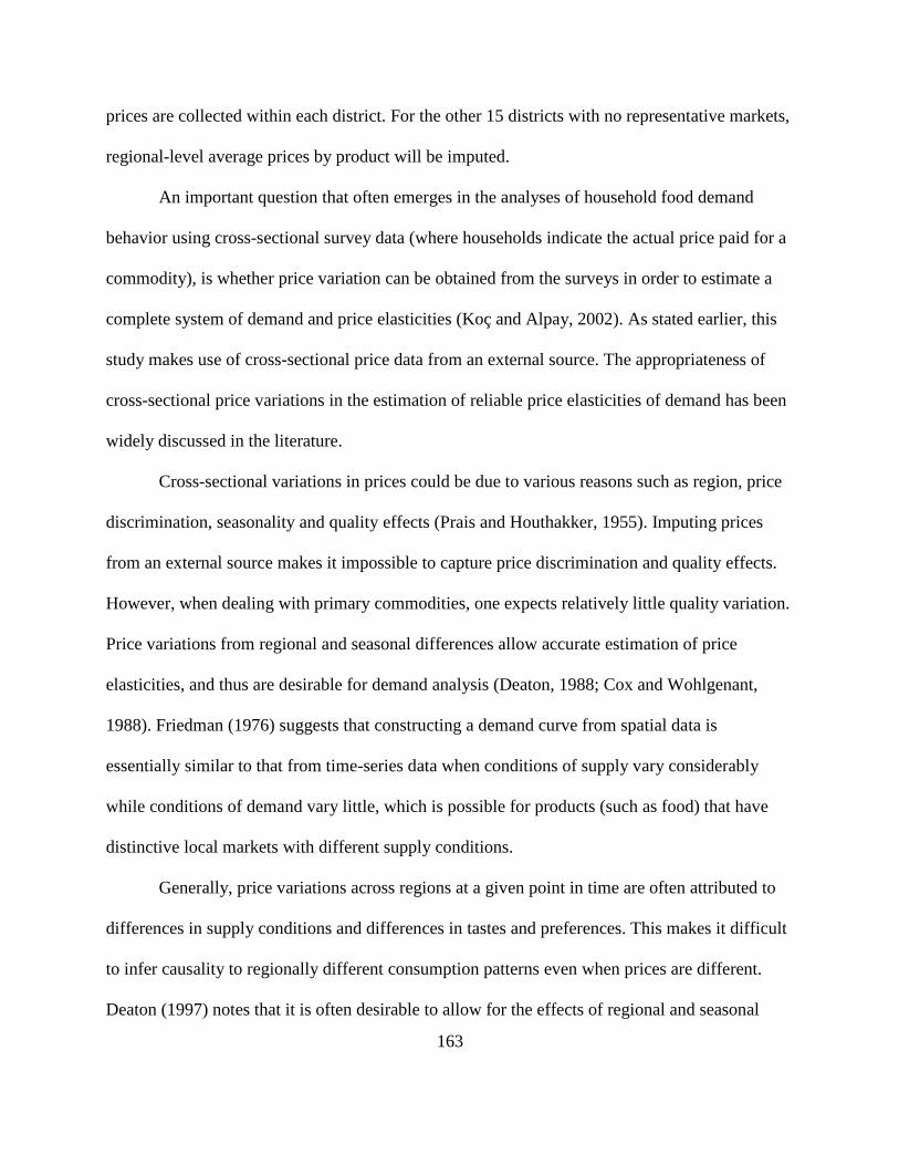
163
prices are collected within each district. For the other 15 districts with no representative markets,
regional-level average prices by product will be imputed.
An important question that often emerges in the analyses of household food demand
behavior using cross-sectional survey data (where households indicate the actual price paid for a
commodity), is whether price variation can be obtained from the surveys in order to estimate a
complete system of demand and price elasticities (Koç and Alpay, 2002). As stated earlier, this
study makes use of cross-sectional price data from an external source. The appropriateness of
cross-sectional price variations in the estimation of reliable price elasticities of demand has been
widely discussed in the literature.
Cross-sectional variations in prices could be due to various reasons such as region, price
discrimination, seasonality and quality effects (Prais and Houthakker, 1955). Imputing prices
from an external source makes it impossible to capture price discrimination and quality effects.
However, when dealing with primary commodities, one expects relatively little quality variation.
Price variations from regional and seasonal differences allow accurate estimation of price
elasticities, and thus are desirable for demand analysis (Deaton, 1988; Cox and Wohlgenant,
1988). Friedman (1976) suggests that constructing a demand curve from spatial data is
essentially similar to that from time-series data when conditions of supply vary considerably
while conditions of demand vary little, which is possible for products (such as food) that have
distinctive local markets with different supply conditions.
Generally, price variations across regions at a given point in time are often attributed to
differences in supply conditions and differences in tastes and preferences. This makes it difficult
to infer causality to regionally different consumption patterns even when prices are different.
Deaton (1997) notes that it is often desirable to allow for the effects of regional and seasonal
164
taste variation in the pattern of demand by entering regional and seasonal dummies into the
regression, so that the price effects on demand are only identified to the degree that there are
multiple observations within regions or that regional prices do not move in parallel across
seasons. Dummy variables will be introduced to isolate changes in demand from differences in
taste and preference from changes in demand from changes in prices.
Deaton (1988) shows that under appropriate separability conditions, one can exploit the
spatial nature of data to back out true price elasticities. The idea is that within a geographic unit
(say district) the prices will be the same, and controlling for district-level fixed effects allows one
to back out the true price elasticities because the real price variation occurs only through the
spatial dimension. Thus, even though the survey is a one shot survey, multiple observations of
prices (district-level) within a region allow us to capture some temporal variability in prices,
which when combined with regional dummy variables permits us to obtain estimates of price
elasticities by income group.
4.3.1.3. Taste and Preferences
Food demand is also strongly influenced by changes in tastes and preferences. Taste and
preferences may change over time (e.g., due to globalization), across regions and with ethnicity.
In a cross-sectional setting, one can capture variations in taste and preferences across regions but
not across time. The use of regional dummy variables enables us to isolate the effect on demand
from differences in taste and preferences (across regions) from other effects.
165
4.3.1.4. Household Socio-demographic Characteristics
Socio-demographic characteristics, such as family size and composition (sex and age), inf1uence
household expenditure patterns and hence are important variables in policy design and analysis.
Teklu (1996) observes that an increase in household size leads to a less than proportional
increase in food consumption. That is, the elasticity of demand for food with respect to size is
less than unity—holding per capita income constant (there are economies of scale in
consumption). Savadogo and Brandt (1988) in urban Burkina Faso showed that such economies
of scale in consumption are larger for high-income groups, who had higher levels of food
consumption, such that the effect of an increase in household size on food consumption is lower
at the margin. Moreover, an increase in household size induces a reallocation of food budget
away from food groups that are income-elastic towards income-inelastic food staples (Savadogo
and Brandt; 1988). Demand patterns may also vary across age (child and adult goods) and sex
within the households.
4.3.1.5. Geographic Location
Geographic regions differ in climatic and infrastructure conditions and hence in the availability
of food and consumption habits (composition of the food basket). Wodon and Zaman (2010)
observe that the distributional impact of rising food prices affects poor households partly based
on where they live, which poses a challenge for policymakers. In the development and targeting
of food safety net interventions to help households cope with the increase in food prices,
policymakers therefore need to identify the hardest hit areas which: a) may not necessarily be
among the poorest in the country; and b) are also not always homogenous in terms of income or
166
other indicators of household vulnerability. Regional dummies are used to isolate geographic
differences in consumption and not just those due to taste and preferences discussed above.
4.3.1.6. Place of Residence
Rural and urban consumption patterns are different due to differences in economic activity and
lifestyle. Rural livelihoods are mostly dependent on agriculture, and rural areas account for much
of the food consumed in Mali. Kelly et al. (2008) note that even in the import-dependent
Sahelian countries, production of coarse grains persists in the rural areas such that while the
urban consumers heavily rely on imported cereal for food, rural households also heavily rely on
traditional coarse grains for their dietary needs and have a lower level of rice consumption. Not
only do rural and urban consumers have different base levels of food consumption (at the
commodity level), but also, time is an important factor that brings about differences in rural and
urban consumption habits. Kennedy and Reardon (1994) found that in urban Burkina Faso the
opportunity cost of women’s time was a major factor in the choice of coarse grains versus-non-
traditional grains. Women who worked outside the home were found to have a strong preference
for rice, which took less time to cook than coarse grains.
Earlier studies of food consumption patterns in the Sahel have focused largely on urban
households, based on the notion that they rely on the market for most of their consumption
because of their lifestyle. Changes in relative prices of food were therefore expected to hurt these
urban consumers more than rural dwellers. According to Kelly et al. (2008), a challenge in the
current food crisis situation is the difficulty to assess the relative vulnerability of urban versus
rural groups. They explained further that because the price hikes to date are greatest on imported
cereals consumed more by urban than rural populations, there is a tendency to think of this more
167
as an urban problem. However, to the extent that these higher prices are transmitted to domestic
cereals and rural markets, or supplies of domestic cereals become tight, the vulnerability may be
as great in rural areas. Thus, a comprehensive understanding of food consumption patterns
requires giving consideration to both rural and urban households.
4.4. Data and Computation of Relevant Variables
The ELIM-2006 HBS data covered 4494 Malian households, urban (1594) and rural (2910), and
9 regions including the district of Bamako. Data were collected on household economic and
socio-demographic characteristics and expenditures by major categories (food and non-food).
Food expenditures are further divided into major food groups (cereals and non-cereals foods) and
cereals expenditures are grouped by cereal crop type. Total consumption expenditures per
expenditure category sums the value of consumption on a given category from all sources
(includes purchases, own-production and from other modes of acquisition). Household adult
equivalents (AE) are calculated by aggregating the determined AE of the respective household
members. The AE for each household member is calculated using the scale: male>14 years=1.0;
female>14=0.8; children=0.5 (Duncan, 1994). Total expenditure on all household expenditure
categories is used as a proxy for household income. Expenditure shares are calculated as the
proportion of each expenditure group in total expenditure for the aggregate group considered.
4.5. Methodological Framework
4.5.1. Commodity Aggregation and Weak Separability
The analysis assumes that consumers’ preferences are weakly separable in order to simplify the
modeling of consumption decisions. Without the assumption of weak separability, the
168
optimization problem is intractable for the consumer if the demand for every commodity is a
function of the prices of all other commodities (Deaton and Muelbauer, 1980). Under this
assumption, the consumer’s simultaneous decision-making process can be broken down into a
three-stage budgeting process. In Stage I, households allocate total budget between food and
non-food items. Conditional on the first stage allocations, in Stage II, households allocate food
expenditure between cereals and non-cereals items. In Stage III, conditional on the second stage
allocations, households allocate cereal expenditures to rice, maize, millet and sorghum. It is thus
assumed that food is weakly separable from non-food commodities and that cereals are weakly
separable from other food groups. The focus of this chapter is Stage III, the reason being that not
only is it more interesting and useful, but also the lack of price/cost information for most non-
food items and non-cereals food items makes the estimation of Stages I and II less feasible.
4.5.2. Modeling Approach
The allocation of total cereals expenditures to specific cereals types (Stage III) is modeled using
the quadratic almost ideal demand system (QUAIDS) proposed by Banks et al. (1997). Unlike its
predecessor, the AIDS of Deaton and Muelbauer (1980), which has budget shares that are linear
functions of log total expenditure and are derived from indirect utility functions that are
themselves linear in log total expenditure (Muelbauer, 1976), the QUAIDS model allows for
non-linearity in the budget shares. As a complete demand system, the QUAIDS allows us to
consistently account for the interdependence in the choices made by households between
different cereal types. By nesting the AIDS model, the QUAIDS model maintains all the relevant
properties of the former (allows for exact aggregation over households and satisfies all the
axioms of choice). In addition to these advantages, the QUAIDS specification allows for more
169
flexibility—expenditure elasticities differ with expenditure levels. This could be a significant
advantage in welfare analysis. It also allows the possibility of normal goods becoming inferior or
vice versa as one move along the expenditure spectrum of households (Bopape, 2006).
4.5.2.1. Model Specification Test
The choice between estimating an AIDS or a QUAIDS model rests on the shape of the Engel
curves. Bopape (2006) developed a parametric quadratic expenditure specification test for
whether the QUAIDS or the AIDS is appropriate for the demand analysis. The test is based on
the fact that the QUAIDS model is rank 3, exactly aggregable and has a coefficient on the linear
expenditure term that is independent of the prices. It involves testing for the statistical
significance of prices in the coefficient on the quadratic expenditure term in the QUAIDS model.
The null hypothesis of the test is that the coefficient on the quadratic expenditure term is
independent of prices across all the budget share equations. This test is a Lagrangian multiplier
(LM) test, and it has the advantage of allowing one to test parametrically if the quadratic
expenditure is necessary without having to estimate the highly non-linear QUAIDS model. This
test is carried out to decide between the QUAIDS and AIDS models.
4.5.2.2. Problems in Demand System Estimation
Zero-expenditure and expenditure endogeneity have been identified as common econometric
issues that arise when cross-sectional data is used to estimate elasticities. These issues need to be
addressed in order to obtain unbiased and efficient price elasticities (Chuang et al. 2005).
170
4.5.2.2.1. Zero-Expenditure
Zero-expenditure arises when a large number of households report zero expenditure for some
commodities/aggregates for which demand is being estimated. This causes a censored dependent
variable problem that leads to biased results if not dealt with. This problem presents an empirical
difficulty because the random disturbances have non-zero means and are correlated with the
exogenous variables (Alfonzo et al. 2006). Tables A4-2 and A4-3 in Appendix show zero
expenditure in the entire sample and by cereal type and by mode of acquisition, respectively.
There is a large proportion of zero expenditure, ranging from 5.1% for rice to 49.8% for maize.
Dropping these households would dramatically reduce the sample size (loss in large number of
degree of freedom) and still give inconsistent estimates. Given that censoring is severe in the
sample, we need a censored system approach.
To address this problem, various estimation methods based on a two-step decision process
initially proposed by Tobin (1958) have been utilized. Heien and Wessells (1990) introduced a
two-step estimation procedure based on Heckman’s (1978) work. However, Shonkwiler and Yen
(S and Y) (1999) demonstrated the inconsistency of Heien and Wessels’ two-step estimation
procedure and they proposed an alternative approach for equation systems with limited
dependent variables. This chapter uses the S and Y approach. Bopape (2006) and Alviola et al.
(2010), Ecker and Quaim (2008), and Tafere et al. (2010) also use this approach for QUAIDS
estimation.
171
4.2.5.2.2. Expenditure Endogeneity (EE)
The problem of EE33 arises when total expenditures are determined jointly with the expenditure
shares of the individual commodities that enter the demand model, making it endogenous in the
expenditure share equations (Blundell and Robin, 1999). This problem may also arise whenever
the household expenditure allocation process is correlated with other unobserved behavior not
captured by the explanatory variables in the budget share equations, because these unobserved
effects would be bundled in the error term. Estimation that ignores EE may lead to inconsistent
demand parameter estimates (Bopape, 2006). This is because a key assumption of regression
analysis is violated—that the mean of the disturbance term is zero and that the disturbance term
is independent of the regressors so that the covariance between the disturbance term and the
independent variables is zero. Bopape (2006) notes that because the problem of EE may affect
the results of the LM test for model specification, it is important to address the problem before
performing the test. Thus, for more reliable results, the LM test should be applied to estimated
budget share equations that have been corrected for potential EE if EE is identified as a problem
with the data.
The augmented regression technique of Hausman (1978) and Blundell and Robin (1999)
has been widely used to deal with the problem of EE. This technique is suitable in a system of
non-linear equations. Barslund (2011) applies this technique to a system of censored demand
33 Most empirical demand analyses do not cover all products that households purchase. As a
result, the practice is to assume separable preferences and estimate a set of conditional demands
for the goods of interest as functions of prices and total expenditure on these goods (Pollak and
Wales, 1969). However, such a practice raises questions regarding the possibility of simultaneity
bias in the budget share equations of the demand model.
172
equations based on the AIDS. Bopape (2006) and Tafera et al. (2010) also use the same
technique to deal with the issue of EE in the context of a QUAIDS model.
The augmented QUAIDS share equations are specified as follows:
𝑤𝑖ℎ = 𝛼𝑖 + 𝛿𝑖ℎ𝑙𝑛𝐴𝐸ℎ + 𝜃𝑖𝑀ℎ + ∑ 𝜌𝑖𝑛𝑅𝐷ℎ
8
𝑛=1
+ ∑ 𝛾𝑖𝑗𝑙𝑛𝑝𝑗ℎ
𝑘
𝑗=1+ 𝛽𝑖𝑙𝑛 [
𝐶𝑋ℎ
𝑎(𝑝ℎ)] +
𝜆𝑖
𝑏(𝑝ℎ){𝑙𝑛 [
𝐶𝑋ℎ
𝑎(𝑝ℎ)]}
2
+ 𝑢𝑖ℎ (4 − 1).
wih is the household budget share for cereal type i. The budget shares are calculated using
food expenditures. pih is the retail price of each cereal type 𝑖̇. C𝑋ℎ is household cereal
expenditure. Dummy variables will capture the effect of a household’s geographic location on
expenditures. RDh, are regional dummies. Mh represents a dummy for place of residence
(urban=1 and rural=0) of a household. The translog price aggregator, a(𝑝ℎ), and the price
aggregator function, b(𝑝ℎ), are functions homogeneous of degree 1 and 0, respectively, in prices.
ln a(𝑝ℎ) and lnb(𝑝ℎ) are specified as translog and Cobb-Douglas equations34.
The theoretical restrictions of homogeneity, adding up and symmetry are the same as
discussed in chapter 3, in addition to:
∑ λ𝑖
𝐾
𝑖=1
= 0 ∀𝑖
34 ln 𝑎(𝑝ℎ) = 𝛼0 + ∑ 𝛼𝑖𝑙𝑛𝑝𝑖ℎ𝑘𝑖=1 +
1
2∑ ∑ 𝛾𝑖𝑗
𝑘𝑗=1
𝑘𝑖=1 𝑙𝑛𝑝𝑖ℎ𝑙𝑛𝑝𝑗ℎ 𝑎𝑛𝑑 𝑏(𝑝ℎ) = ∏ 𝑝𝑖ℎ
𝛽𝑖𝑘𝑖=1 .
For commodities i=1,…k.
173
To deal with the problem of EE, assume that the error terms have an orthogonal
decomposition
𝑢𝑠𝑖 = 𝜌𝑠𝜏𝑠𝑖 + 휀𝑠𝑖 (4 − 2)
𝜏𝑠𝑖 are the residuals from the regression of total cereal expenditure on the set of instruments and
explanatory variables. 휀𝑠𝑖 is normally distributed. The parameter 𝜌𝑠 provides a test of exogeneity
of total cereal expenditure for each consumption share and should be equal to zero if the cereal
expenditure is exogenous.
To deal with the problem of censoring, following the S and Y approach, consider the
dichotomous variable
𝑑𝑖ℎ = 1 𝑖𝑓 𝜎𝑖𝑧𝑖ℎ + 𝑣𝑖ℎ > 0 ; 𝑎𝑛𝑑 𝑑𝑖ℎ = 0 𝑜𝑡ℎ𝑒𝑟𝑤𝑖𝑠𝑒 (4 − 3)
Where 𝜎𝑖 is a vector of coefficients, 𝑧𝑖ℎ a vector of explanatory variables and 𝑣𝑖ℎ is the equation-
specific error term, which is distributed normally (0,1).
The observed expenditure shares for the hth household are given by:
𝑤𝑖ℎ𝑜𝑏𝑠 = (𝑤𝑖ℎ + 𝜌𝑠𝜏𝑠𝑖) ∙ 𝑑𝑖ℎ (4 − 4)
Consistent parameters in equation 4-1 can be obtained by estimating
𝑤𝑖ℎ𝑜𝑏𝑠 = Ф(�̂�𝑖𝑧𝑖ℎ)(𝑤𝑖ℎ + 𝜌𝑠𝜏𝑠𝑖) + 𝜋𝑖𝜙(�̂�𝑖𝑧𝑖ℎ) + 𝜉𝑖ℎ (4 − 5)
Where σ̂izih are predicted indices from the first-step probit estimation of the equation in
(4-3) and Ф and ϕ are respectively the standard normal cumulative distribution (cdf) and
probability density (pdf) functions. Unlike in the conventional system specification without
censoring, the deterministic components on the right hand side of equation (4-5) do not add up to
unity across all equations of the system, and so the error terms in the estimation form do not add
up to zero (Yen et al., 2002). As a result, the usual procedure of imposing the adding-up
174
restriction on the system and dropping one equation is not valid. Therefore, with censoring,
equation (4-5) is estimated correctly when using the entire set of n equations (Yen et al., 2002).
The expressions for the elasticities following Banks et al. (1997) are simplified as
follows:
𝜇𝑖 ≡𝜕𝑤𝑖ℎ
𝑜𝑏𝑠
𝜕𝑙𝑛𝐶𝑋ℎ= Ф(�̂�𝑖𝑧𝑖ℎ) [𝛽𝑖 +
2𝜆𝑖
𝑏(𝑝ℎ){𝑙𝑛 [
𝐶𝑋ℎ
𝑎(𝑝ℎ)]}] (4 − 6)
𝜇𝑖𝑖 ≡𝜕𝑤𝑖ℎ
𝑜𝑏𝑠
𝜕𝑙𝑛𝑝𝑖= Ф(�̂�𝑖𝑧𝑖ℎ) ⌈𝛾𝑖𝑗 − 𝜇𝑖 (𝛼𝑖 + ∑ 𝛾𝑗𝑙
𝐾
𝑙=1
𝑙𝑛𝑝𝑙ℎ) −𝜆𝑖𝛽𝑗
𝑏(𝑝ℎ){𝑙𝑛 [
𝐶𝑋ℎ
𝑎(𝑝ℎ)]}
2
⌉ (4 − 7)
Expressing the formula for expenditure elasticities in terms of 𝜇𝑖:
𝑒𝑖 =𝜇𝑖
𝑤𝑖 + 1 (4 − 8)
Similarly, the Marshallian or uncompensated elasticities of demand can be expressed as follows:
𝑒𝑖𝑗𝑢 =
𝜇𝑖𝑗
𝑤𝑖− 𝛿𝑖𝑗 (4 − 9)
Where δij is the Kronecker delta equating 1 if i=j and 0 otherwise. The Hicksian or compensated
elasticities can be derived as thus using Slutsky equation
eijc = eij
u + wiei (4 − 10)
4.6. Estimation Method
The complete estimation procedure for Stage III follows this pattern: in step one, a test for
endogeneity of the total cereal expenditure is carried out using instrumental variables; in step
two, a model specification test is carried out to determine the appropriateness of the AIDS versus
QUAIDS model; in step 3 the system (4-3) is estimated by multivariate probit and the pdfs and
cdfs are computed; in step 4 the system in 4-5 is estimated using Non-linear, Seemingly
Unrelated Regression (NLSUR) in STATA. To capture differences in expenditure patterns across
income groups, households will be divided into income groups and the consumption behavior for
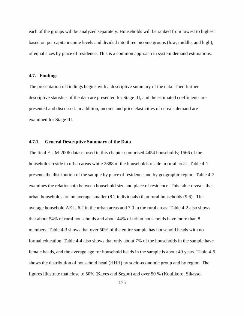
175
each of the groups will be analyzed separately. Households will be ranked from lowest to highest
based on per capita income levels and divided into three income groups (low, middle, and high),
of equal sizes by place of residence. This is a common approach in system demand estimations.
4.7. Findings
The presentation of findings begins with a descriptive summary of the data. Then further
descriptive statistics of the data are presented for Stage III, and the estimated coefficients are
presented and discussed. In addition, income and price elasticities of cereals demand are
examined for Stage III.
4.7.1. General Descriptive Summary of the Data
The final ELIM-2006 dataset used in this chapter comprised 4454 households; 1566 of the
households reside in urban areas while 2888 of the households reside in rural areas. Table 4-1
presents the distribution of the sample by place of residence and by geographic region. Table 4-2
examines the relationship between household size and place of residence. This table reveals that
urban households are on average smaller (8.2 individuals) than rural households (9.6). The
average household AE is 6.2 in the urban areas and 7.0 in the rural areas. Table 4-2 also shows
that about 54% of rural households and about 44% of urban households have more than 8
members. Table 4-3 shows that over 50% of the entire sample has household heads with no
formal education. Table 4-4 also shows that only about 7% of the households in the sample have
female heads, and the average age for household heads in the sample is about 49 years. Table 4-5
shows the distribution of household head (HHH) by socio-economic group and by region. The
figures illustrate that close to 50% (Kayes and Segou) and over 50 % (Koulikoro, Sikasso,

176
Mopti, Tombouctou, and Kidal) of the household heads are independent farmers. The District of
Bamako, as expected, has the smallest number of cases where household heads are independent
farmers.
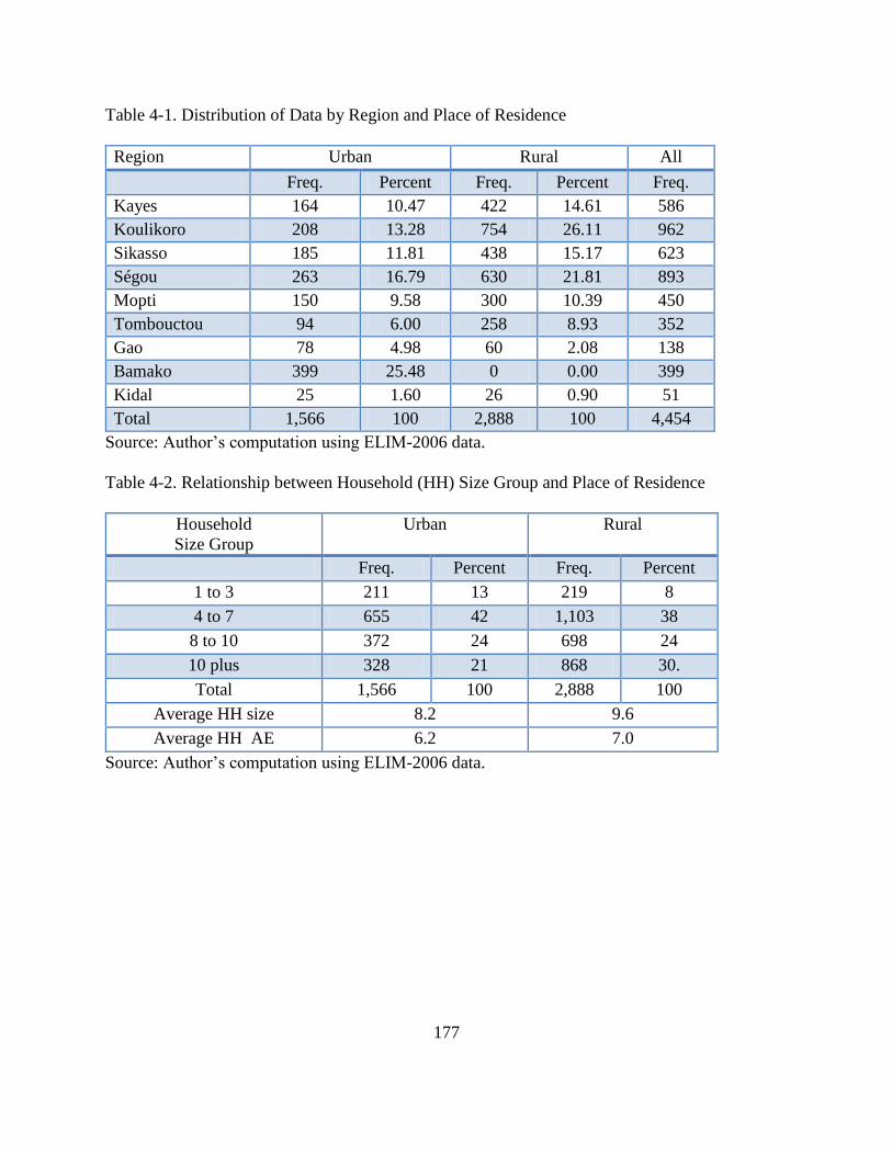
177
Table 4-1. Distribution of Data by Region and Place of Residence
Region Urban Rural All
Freq. Percent Freq. Percent Freq.
Kayes 164 10.47 422 14.61 586
Koulikoro 208 13.28 754 26.11 962
Sikasso 185 11.81 438 15.17 623
Ségou 263 16.79 630 21.81 893
Mopti 150 9.58 300 10.39 450
Tombouctou 94 6.00 258 8.93 352
Gao 78 4.98 60 2.08 138
Bamako 399 25.48 0 0.00 399
Kidal 25 1.60 26 0.90 51
Total 1,566 100 2,888 100 4,454
Source: Author’s computation using ELIM-2006 data.
Table 4-2. Relationship between Household (HH) Size Group and Place of Residence
Household
Size Group
Urban Rural
Freq. Percent Freq. Percent
1 to 3 211 13 219 8
4 to 7 655 42 1,103 38
8 to 10 372 24 698 24
10 plus 328 21 868 30.
Total 1,566 100 2,888 100
Average HH size 8.2 9.6
Average HH AE 6.2 7.0
Source: Author’s computation using ELIM-2006 data.
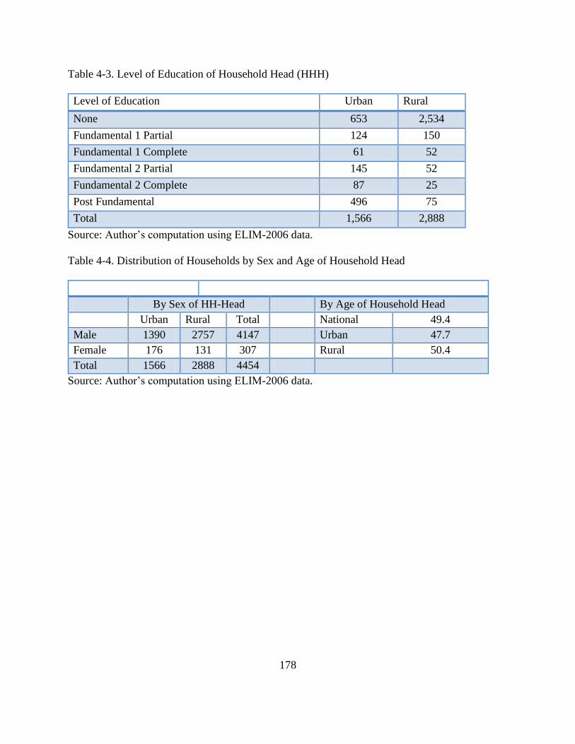
178
Table 4-3. Level of Education of Household Head (HHH)
Level of Education Urban Rural
None 653 2,534
Fundamental 1 Partial 124 150
Fundamental 1 Complete 61 52
Fundamental 2 Partial 145 52
Fundamental 2 Complete 87 25
Post Fundamental 496 75
Total 1,566 2,888
Source: Author’s computation using ELIM-2006 data.
Table 4-4. Distribution of Households by Sex and Age of Household Head
By Sex of HH-Head By Age of Household Head
Urban Rural Total National 49.4
Male 1390 2757 4147 Urban 47.7
Female 176 131 307 Rural 50.4
Total 1566 2888 4454
Source: Author’s computation using ELIM-2006 data.
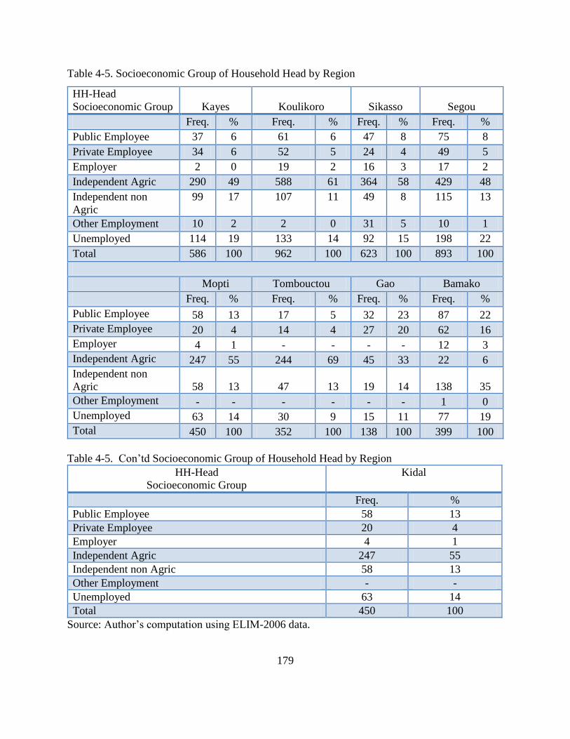
179
Table 4-5. Socioeconomic Group of Household Head by Region
HH-Head
Socioeconomic Group
Kayes
Koulikoro
Sikasso
Segou
Freq. % Freq. % Freq. % Freq. %
Public Employee 37 6 61 6 47 8 75 8
Private Employee 34 6 52 5 24 4 49 5
Employer 2 0 19 2 16 3 17 2
Independent Agric 290 49 588 61 364 58 429 48
Independent non
Agric
99 17 107 11 49 8 115 13
Other Employment 10 2 2 0 31 5 10 1
Unemployed 114 19 133 14 92 15 198 22
Total 586 100 962 100 623 100 893 100
Mopti Tombouctou Gao Bamako
Freq. % Freq. % Freq. % Freq. %
Public Employee 58 13 17 5 32 23 87 22
Private Employee 20 4 14 4 27 20 62 16
Employer 4 1 - - - - 12 3
Independent Agric 247 55 244 69 45 33 22 6
Independent non
Agric 58 13 47 13 19 14 138 35
Other Employment - - - - - - 1 0
Unemployed 63 14 30 9 15 11 77 19
Total 450 100 352 100 138 100 399 100
Table 4-5. Con’td Socioeconomic Group of Household Head by Region
HH-Head
Socioeconomic Group
Kidal
Freq. %
Public Employee 58 13
Private Employee 20 4
Employer 4 1
Independent Agric 247 55
Independent non Agric 58 13
Other Employment - -
Unemployed 63 14
Total 450 100
Source: Author’s computation using ELIM-2006 data.
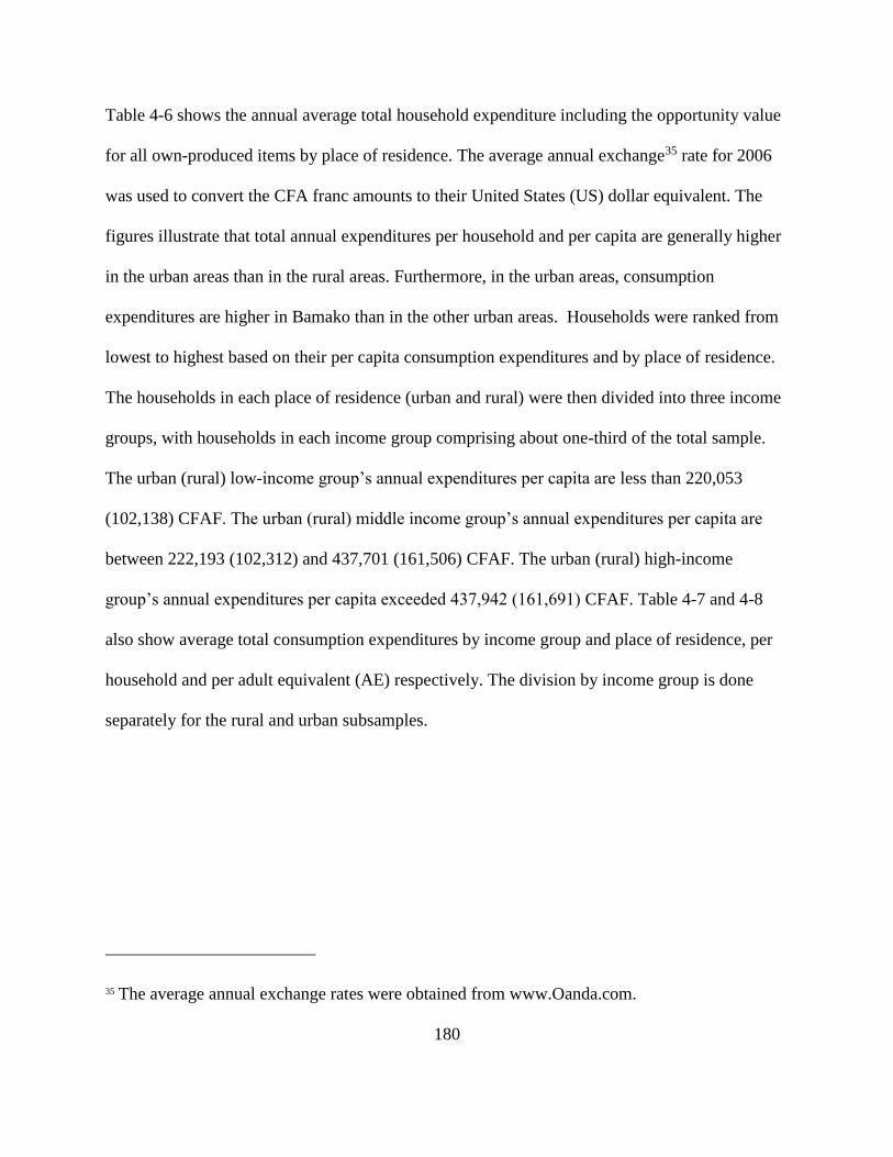
180
Table 4-6 shows the annual average total household expenditure including the opportunity value
for all own-produced items by place of residence. The average annual exchange35 rate for 2006
was used to convert the CFA franc amounts to their United States (US) dollar equivalent. The
figures illustrate that total annual expenditures per household and per capita are generally higher
in the urban areas than in the rural areas. Furthermore, in the urban areas, consumption
expenditures are higher in Bamako than in the other urban areas. Households were ranked from
lowest to highest based on their per capita consumption expenditures and by place of residence.
The households in each place of residence (urban and rural) were then divided into three income
groups, with households in each income group comprising about one-third of the total sample.
The urban (rural) low-income group’s annual expenditures per capita are less than 220,053
(102,138) CFAF. The urban (rural) middle income group’s annual expenditures per capita are
between 222,193 (102,312) and 437,701 (161,506) CFAF. The urban (rural) high-income
group’s annual expenditures per capita exceeded 437,942 (161,691) CFAF. Table 4-7 and 4-8
also show average total consumption expenditures by income group and place of residence, per
household and per adult equivalent (AE) respectively. The division by income group is done
separately for the rural and urban subsamples.
35 The average annual exchange rates were obtained from www.Oanda.com.
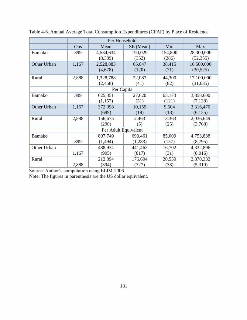
181
Table 4-6. Annual Average Total Consumption Expenditures (CFAF) by Place of Residence
Per Household
Obs Mean SE (Mean) Min Max
Bamako 399 4,534,634
(8,389)
190,029
(352)
154,800
(286)
28,300,000
(52,355)
Other Urban 1,167 2,528,883
(4,678)
65,047
(120)
38,415
(71)
16,500,000
(30,525)
Rural 2,888 1,328,788
(2,458)
22,087
(41)
44,300
(82)
17,100,000
(31,635)
Per Capita
Bamako 399 625,351
(1,157)
27,620
(51)
65,173
(121)
3,858,600
(7,138)
Other Urban 1,167 372,098
(689)
10,159
(19)
9,604
(18)
3,316,470
(6,135)
Rural 2,888 156,675
(290)
2,463
(5)
13,363
(25)
2,036,649
(3,768)
Per Adult Equivalent
Bamako
399
807,749
(1,494)
693,461
(1,283)
85,009
(157)
4,753,838
(8,795)
Other Urban
1,167
488,934
(905)
441,462
(817)
16,702
(31)
4,332,896
(8,016)
Rural
2,888
212,894
(394)
176,604
(327)
20,559
(38)
2,870,332
(5,310)
Source: Author’s computation using ELIM-2006.
Note: The figures in parenthesis are the US dollar equivalent.
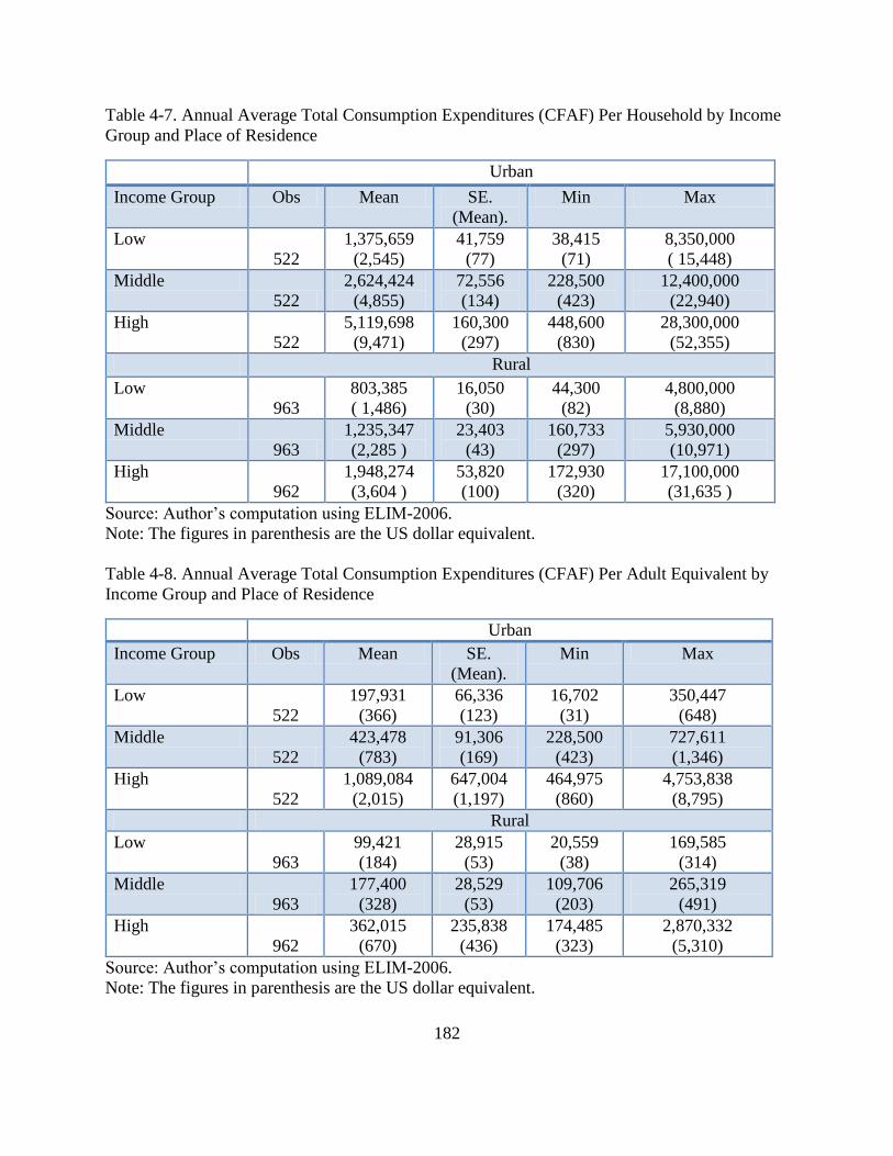
182
Table 4-7. Annual Average Total Consumption Expenditures (CFAF) Per Household by Income
Group and Place of Residence
Urban
Income Group Obs Mean SE.
(Mean).
Min Max
Low
522
1,375,659
(2,545)
41,759
(77)
38,415
(71)
8,350,000
( 15,448)
Middle
522
2,624,424
(4,855)
72,556
(134)
228,500
(423)
12,400,000
(22,940)
High
522
5,119,698
(9,471)
160,300
(297)
448,600
(830)
28,300,000
(52,355)
Rural
Low
963
803,385
( 1,486)
16,050
(30)
44,300
(82)
4,800,000
(8,880)
Middle
963
1,235,347
(2,285 )
23,403
(43)
160,733
(297)
5,930,000
(10,971)
High
962
1,948,274
(3,604 )
53,820
(100)
172,930
(320)
17,100,000
(31,635 )
Source: Author’s computation using ELIM-2006.
Note: The figures in parenthesis are the US dollar equivalent.
Table 4-8. Annual Average Total Consumption Expenditures (CFAF) Per Adult Equivalent by
Income Group and Place of Residence
Urban
Income Group Obs Mean SE.
(Mean).
Min Max
Low
522
197,931
(366)
66,336
(123)
16,702
(31)
350,447
(648)
Middle
522
423,478
(783)
91,306
(169)
228,500
(423)
727,611
(1,346)
High
522
1,089,084
(2,015)
647,004
(1,197)
464,975
(860)
4,753,838
(8,795)
Rural
Low
963
99,421
(184)
28,915
(53)
20,559
(38)
169,585
(314)
Middle
963
177,400
(328)
28,529
(53)
109,706
(203)
265,319
(491)
High
962
362,015
(670)
235,838
(436)
174,485
(323)
2,870,332
(5,310)
Source: Author’s computation using ELIM-2006.
Note: The figures in parenthesis are the US dollar equivalent.
183
The households’ total food expenditure includes expenditures on food purchased and the
value of consumption from own production. Table 4-9 shows average annual food and non-food
expenditures by place of residence in CFAF. The figures reveal that food and non-food
expenditures are higher for Bamako than for other urban areas and rural areas in both per
household and per adult equivalent terms. Average annual food expenditure per AE for Bamako
is 212,571 CFAF, compared to 166,842 CFAF for other urban areas and 113,442 CFAF for rural
areas. Table 4-10 also shows the distribution of food and non-food expenditures by income
group and by place of residence. We observe an increase in food and non-food expenditure per
household and per household adult equivalent from the low to the high income group within the
urban and rural locations. Also, urban per AE food expenditures are higher than rural per AE
food expenditures across all income groups.
Table 4-9. Average Annual Food and Non-Food Expenditure (CFAF) by Place of Residence
Bamako
(N=399)
Other Urban
(N=1167)
Rural
(N=2888)
Per Household
Food 1,243,871
(2,301)
907,997
(1,680 )
705,161
(1,305 )
Non-food 3,290,763
(6,088)
1,620,887
(2,999)
623,627
(1,154 )
Per Adult Equivalent
Food 212,571
(393)
166,842
(309)
113,442
(210)
Non-food 595,178
(1,101)
322,092
(596)
99,452
(184)
Source: Author’s computation using ELIM-2006.
The figures in parenthesis are the US dollar equivalent.
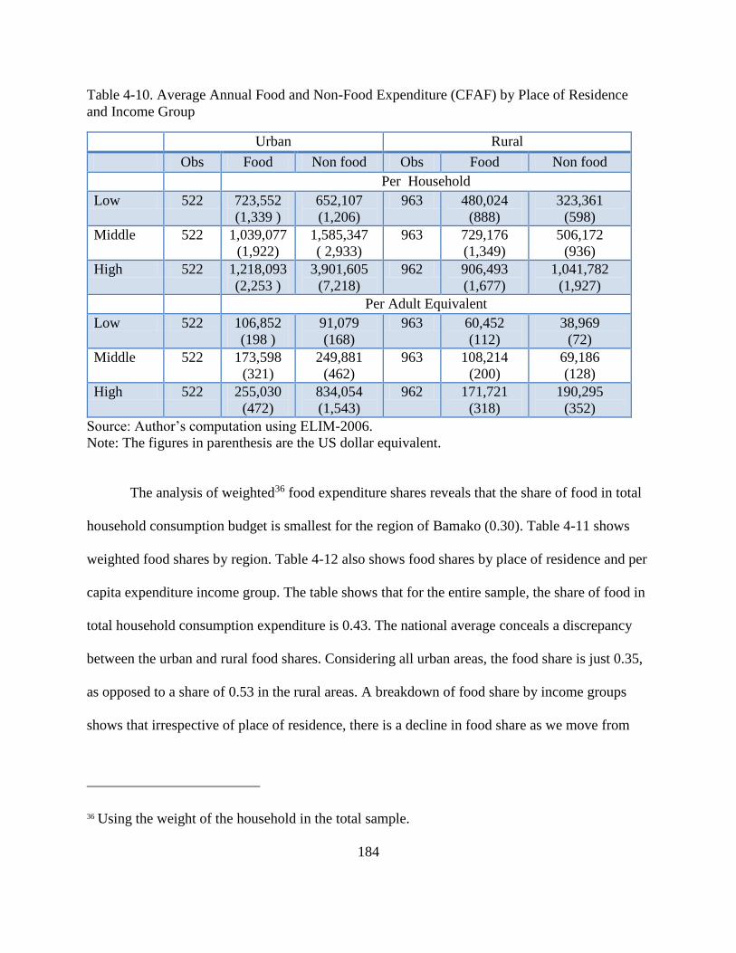
184
Table 4-10. Average Annual Food and Non-Food Expenditure (CFAF) by Place of Residence
and Income Group
Urban Rural
Obs Food Non food Obs Food Non food
Per Household
Low 522 723,552
(1,339 )
652,107
(1,206)
963 480,024
(888)
323,361
(598)
Middle 522 1,039,077
(1,922)
1,585,347
( 2,933)
963 729,176
(1,349)
506,172
(936)
High 522 1,218,093
(2,253 )
3,901,605
(7,218)
962 906,493
(1,677)
1,041,782
(1,927)
Per Adult Equivalent
Low 522 106,852
(198 )
91,079
(168)
963 60,452
(112)
38,969
(72)
Middle 522 173,598
(321)
249,881
(462)
963 108,214
(200)
69,186
(128)
High 522 255,030
(472)
834,054
(1,543)
962 171,721
(318)
190,295
(352)
Source: Author’s computation using ELIM-2006.
Note: The figures in parenthesis are the US dollar equivalent.
The analysis of weighted36 food expenditure shares reveals that the share of food in total
household consumption budget is smallest for the region of Bamako (0.30). Table 4-11 shows
weighted food shares by region. Table 4-12 also shows food shares by place of residence and per
capita expenditure income group. The table shows that for the entire sample, the share of food in
total household consumption expenditure is 0.43. The national average conceals a discrepancy
between the urban and rural food shares. Considering all urban areas, the food share is just 0.35,
as opposed to a share of 0.53 in the rural areas. A breakdown of food share by income groups
shows that irrespective of place of residence, there is a decline in food share as we move from
36 Using the weight of the household in the total sample.
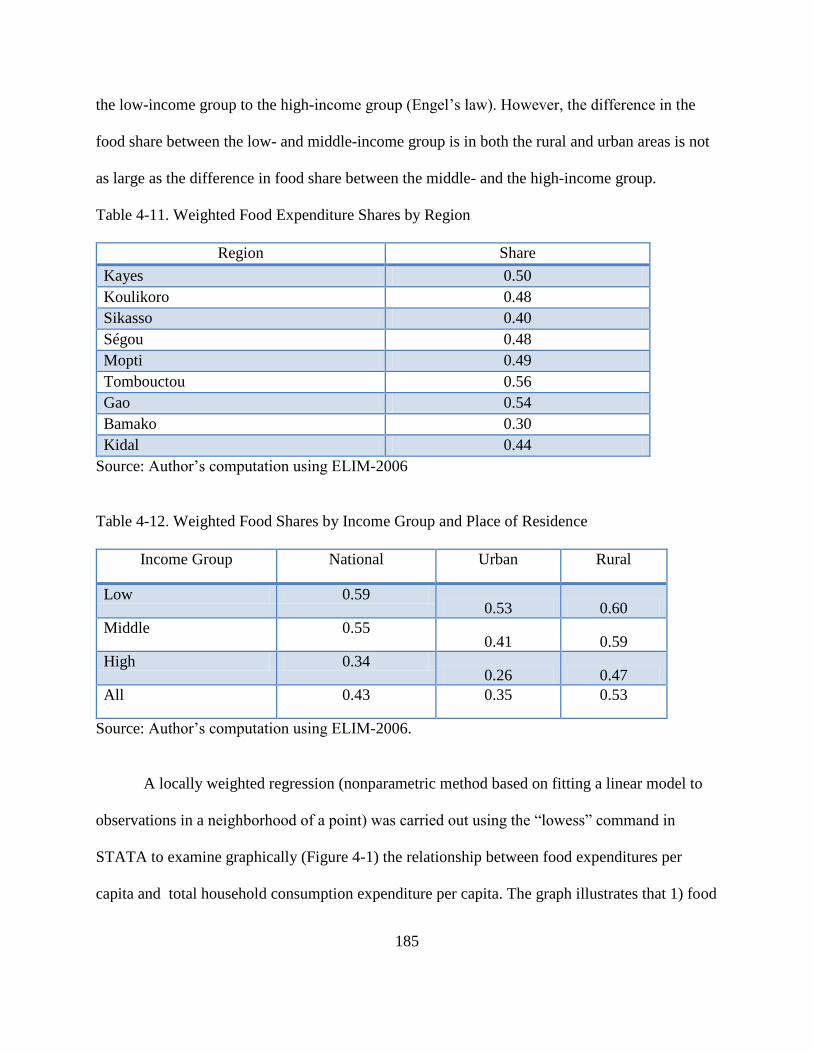
185
the low-income group to the high-income group (Engel’s law). However, the difference in the
food share between the low- and middle-income group is in both the rural and urban areas is not
as large as the difference in food share between the middle- and the high-income group.
Table 4-11. Weighted Food Expenditure Shares by Region
Region Share
Kayes 0.50
Koulikoro 0.48
Sikasso 0.40
Ségou 0.48
Mopti 0.49
Tombouctou 0.56
Gao 0.54
Bamako 0.30
Kidal 0.44
Source: Author’s computation using ELIM-2006
Table 4-12. Weighted Food Shares by Income Group and Place of Residence
Income Group National Urban Rural
Low 0.59 0.53 0.60
Middle 0.55 0.41 0.59
High 0.34 0.26 0.47
All 0.43 0.35 0.53
Source: Author’s computation using ELIM-2006.
A locally weighted regression (nonparametric method based on fitting a linear model to
observations in a neighborhood of a point) was carried out using the “lowess” command in
STATA to examine graphically (Figure 4-1) the relationship between food expenditures per
capita and total household consumption expenditure per capita. The graph illustrates that 1) food
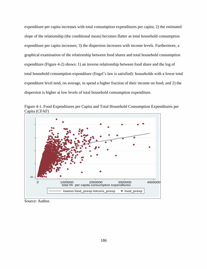
186
expenditure per capita increases with total consumption expenditures per capita; 2) the estimated
slope of the relationship (the conditional mean) becomes flatter as total household consumption
expenditure per capita increases; 3) the dispersion increases with income levels. Furthermore, a
graphical examination of the relationship between food shares and total household consumption
expenditure (Figure 4-2) shows: 1) an inverse relationship between food share and the log of
total household consumption expenditure (Engel’s law is satisfied): households with a lower total
expenditure level tend, on average, to spend a higher fraction of their income on food; and 2) the
dispersion is higher at low levels of total household consumption expenditure.
Figure 4-1. Food Expenditures per Capita and Total Household Consumption Expenditures per
Capita (CFAF)
Source: Author.
0
1000
0020
0000
3000
0040
0000
0 1000000 2000000 3000000 4000000 total hh per capita consumption expenditures
lowess food_pcexp totcons_pcexp food_pcexp
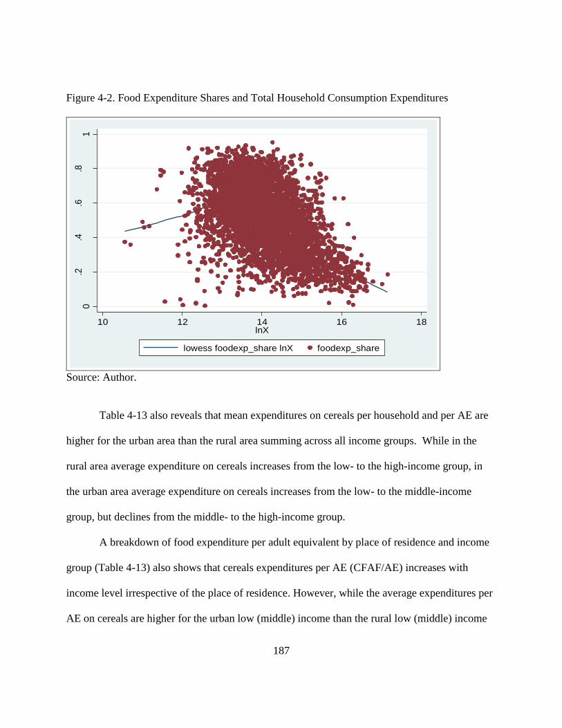
187
Figure 4-2. Food Expenditure Shares and Total Household Consumption Expenditures
Source: Author.
Table 4-13 also reveals that mean expenditures on cereals per household and per AE are
higher for the urban area than the rural area summing across all income groups. While in the
rural area average expenditure on cereals increases from the low- to the high-income group, in
the urban area average expenditure on cereals increases from the low- to the middle-income
group, but declines from the middle- to the high-income group.
A breakdown of food expenditure per adult equivalent by place of residence and income
group (Table 4-13) also shows that cereals expenditures per AE (CFAF/AE) increases with
income level irrespective of the place of residence. However, while the average expenditures per
AE on cereals are higher for the urban low (middle) income than the rural low (middle) income
0.2
.4.6
.81
10 12 14 16 18lnX
lowess foodexp_share lnX foodexp_share
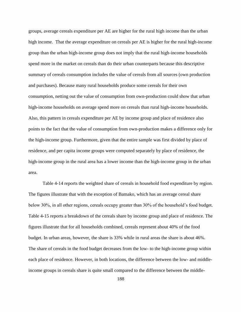
188
groups, average cereals expenditure per AE are higher for the rural high income than the urban
high income. That the average expenditure on cereals per AE is higher for the rural high-income
group than the urban high-income group does not imply that the rural high-income households
spend more in the market on cereals than do their urban counterparts because this descriptive
summary of cereals consumption includes the value of cereals from all sources (own production
and purchases). Because many rural households produce some cereals for their own
consumption, netting out the value of consumption from own-production could show that urban
high-income households on average spend more on cereals than rural high-income households.
Also, this pattern in cereals expenditure per AE by income group and place of residence also
points to the fact that the value of consumption from own-production makes a difference only for
the high-income group. Furthermore, given that the entire sample was first divided by place of
residence, and per capita income groups were computed separately by place of residence, the
high-income group in the rural area has a lower income than the high-income group in the urban
area.
Table 4-14 reports the weighted share of cereals in household food expenditure by region.
The figures illustrate that with the exception of Bamako, which has an average cereal share
below 30%, in all other regions, cereals occupy greater than 30% of the household’s food budget.
Table 4-15 reports a breakdown of the cereals share by income group and place of residence. The
figures illustrate that for all households combined, cereals represent about 40% of the food
budget. In urban areas, however, the share is 33% while in rural areas the share is about 46%.
The share of cereals in the food budget decreases from the low- to the high-income group within
each place of residence. However, in both locations, the difference between the low- and middle-
income groups in cereals share is quite small compared to the difference between the middle-
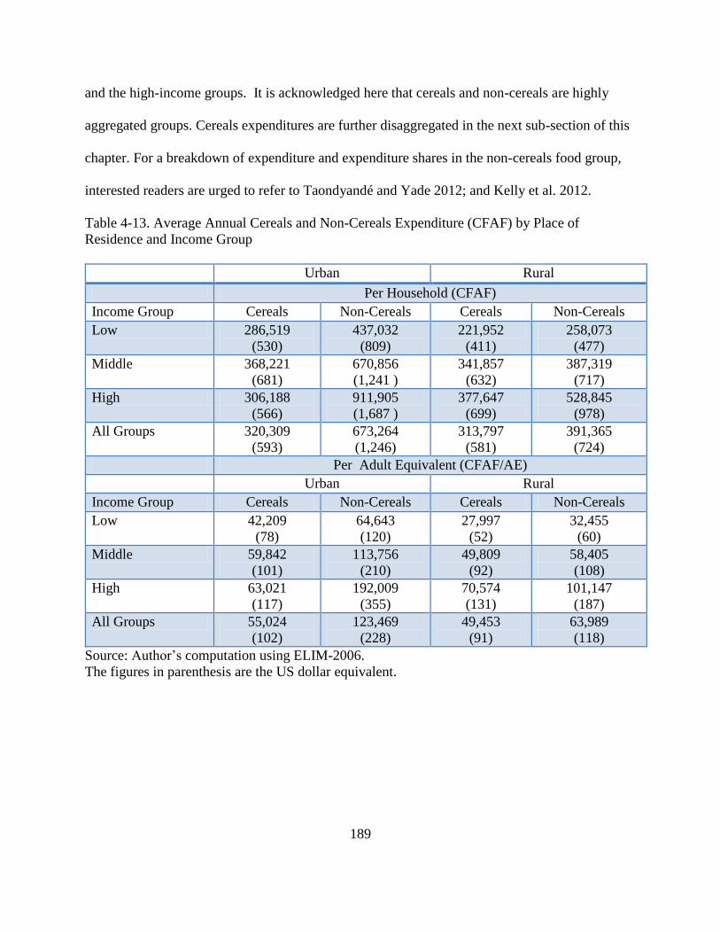
189
and the high-income groups. It is acknowledged here that cereals and non-cereals are highly
aggregated groups. Cereals expenditures are further disaggregated in the next sub-section of this
chapter. For a breakdown of expenditure and expenditure shares in the non-cereals food group,
interested readers are urged to refer to Taondyandé and Yade 2012; and Kelly et al. 2012.
Table 4-13. Average Annual Cereals and Non-Cereals Expenditure (CFAF) by Place of
Residence and Income Group
Urban Rural
Per Household (CFAF)
Income Group Cereals Non-Cereals Cereals Non-Cereals
Low 286,519
(530)
437,032
(809)
221,952
(411)
258,073
(477)
Middle 368,221
(681)
670,856
(1,241 )
341,857
(632)
387,319
(717)
High 306,188
(566)
911,905
(1,687 )
377,647
(699)
528,845
(978)
All Groups 320,309
(593)
673,264
(1,246)
313,797
(581)
391,365
(724)
Per Adult Equivalent (CFAF/AE)
Urban Rural
Income Group Cereals Non-Cereals Cereals Non-Cereals
Low 42,209
(78)
64,643
(120)
27,997
(52)
32,455
(60)
Middle 59,842
(101)
113,756
(210)
49,809
(92)
58,405
(108)
High 63,021
(117)
192,009
(355)
70,574
(131)
101,147
(187)
All Groups 55,024
(102)
123,469
(228)
49,453
(91)
63,989
(118)
Source: Author’s computation using ELIM-2006.
The figures in parenthesis are the US dollar equivalent.
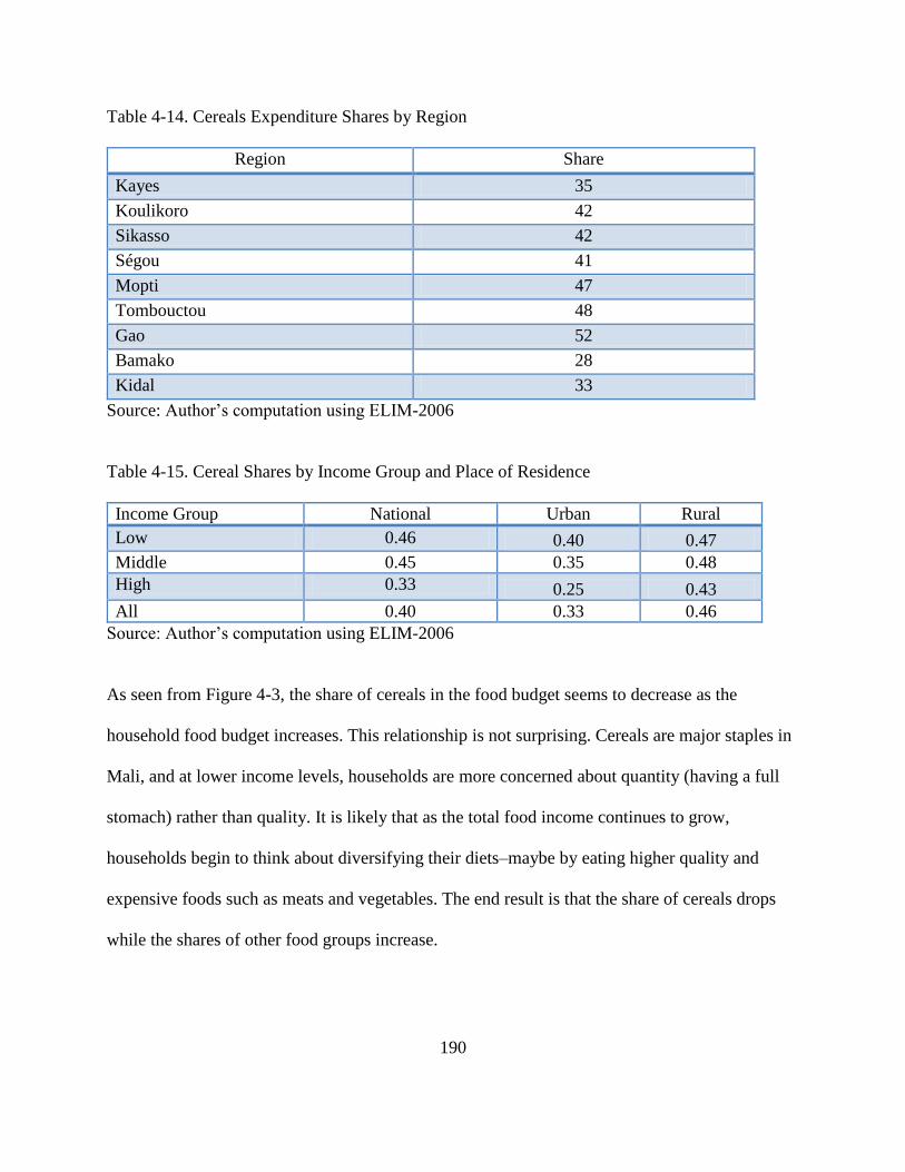
190
Table 4-14. Cereals Expenditure Shares by Region
Region Share
Kayes 35
Koulikoro 42
Sikasso 42
Ségou 41
Mopti 47
Tombouctou 48
Gao 52
Bamako 28
Kidal 33
Source: Author’s computation using ELIM-2006
Table 4-15. Cereal Shares by Income Group and Place of Residence
Income Group National Urban Rural
Low 0.46 0.40 0.47
Middle 0.45 0.35 0.48
High 0.33 0.25 0.43
All 0.40 0.33 0.46
Source: Author’s computation using ELIM-2006
As seen from Figure 4-3, the share of cereals in the food budget seems to decrease as the
household food budget increases. This relationship is not surprising. Cereals are major staples in
Mali, and at lower income levels, households are more concerned about quantity (having a full
stomach) rather than quality. It is likely that as the total food income continues to grow,
households begin to think about diversifying their diets–maybe by eating higher quality and
expensive foods such as meats and vegetables. The end result is that the share of cereals drops
while the shares of other food groups increase.
191
Figure 4-3. Total Household Food Expenditure and the Share of Cereals in Food Budget
Source: Author’s computation using ELIM-2006.
Note: Households with zero expenditure on all cereals were excluded.
As mentioned above, households get their food from three main sources: own-production,
purchases from the market and “others” (gifts and ceremonies). The ELIM-2006 household
budget survey reports consumption expenditures by mode of acquisition. However, it is not clear
from the survey data whether consumption from own-production was valued at market prices or
not. Furthermore, for purchased food expenditures, the data do not make a distinction between
cereals consumption away from home and purchased food prepared at home. Summary statistics
for individual cereals consumption will include the value of consumption from all the different
sources of cereals supply.
Table 4-16 below reports average annual expenditures per adult equivalent by cereal type
and place of residence. National annual average expenditures are 25,125 CFAF/AE (46 US$/AE)
0.2
.4.6
.81
10 12 14 16lnFX
lowess cerealexp_share lnFX cerealexp_share
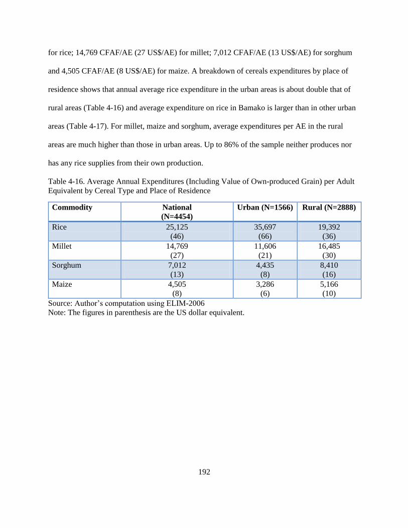
192
for rice; 14,769 CFAF/AE (27 US$/AE) for millet; 7,012 CFAF/AE (13 US$/AE) for sorghum
and 4,505 CFAF/AE (8 US$/AE) for maize. A breakdown of cereals expenditures by place of
residence shows that annual average rice expenditure in the urban areas is about double that of
rural areas (Table 4-16) and average expenditure on rice in Bamako is larger than in other urban
areas (Table 4-17). For millet, maize and sorghum, average expenditures per AE in the rural
areas are much higher than those in urban areas. Up to 86% of the sample neither produces nor
has any rice supplies from their own production.
Table 4-16. Average Annual Expenditures (Including Value of Own-produced Grain) per Adult
Equivalent by Cereal Type and Place of Residence
Commodity National
(N=4454)
Urban (N=1566) Rural (N=2888)
Rice 25,125
(46)
35,697
(66)
19,392
(36)
Millet 14,769
(27)
11,606
(21)
16,485
(30)
Sorghum 7,012
(13)
4,435
(8)
8,410
(16)
Maize 4,505
(8)
3,286
(6)
5,166
(10)
Source: Author’s computation using ELIM-2006
Note: The figures in parenthesis are the US dollar equivalent.
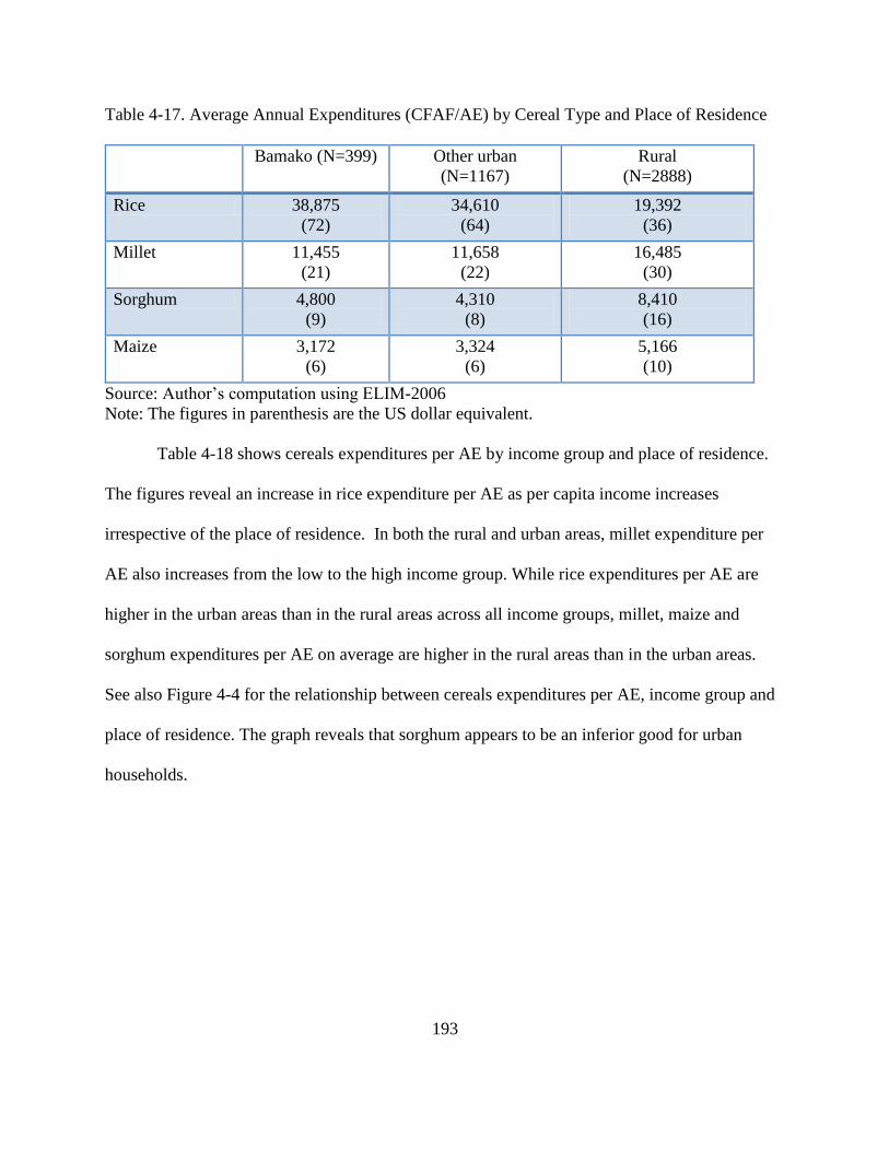
193
Table 4-17. Average Annual Expenditures (CFAF/AE) by Cereal Type and Place of Residence
Bamako (N=399) Other urban
(N=1167)
Rural
(N=2888)
Rice 38,875
(72)
34,610
(64)
19,392
(36)
Millet 11,455
(21)
11,658
(22)
16,485
(30)
Sorghum 4,800
(9)
4,310
(8)
8,410
(16)
Maize 3,172
(6)
3,324
(6)
5,166
(10)
Source: Author’s computation using ELIM-2006
Note: The figures in parenthesis are the US dollar equivalent.
Table 4-18 shows cereals expenditures per AE by income group and place of residence.
The figures reveal an increase in rice expenditure per AE as per capita income increases
irrespective of the place of residence. In both the rural and urban areas, millet expenditure per
AE also increases from the low to the high income group. While rice expenditures per AE are
higher in the urban areas than in the rural areas across all income groups, millet, maize and
sorghum expenditures per AE on average are higher in the rural areas than in the urban areas.
See also Figure 4-4 for the relationship between cereals expenditures per AE, income group and
place of residence. The graph reveals that sorghum appears to be an inferior good for urban
households.
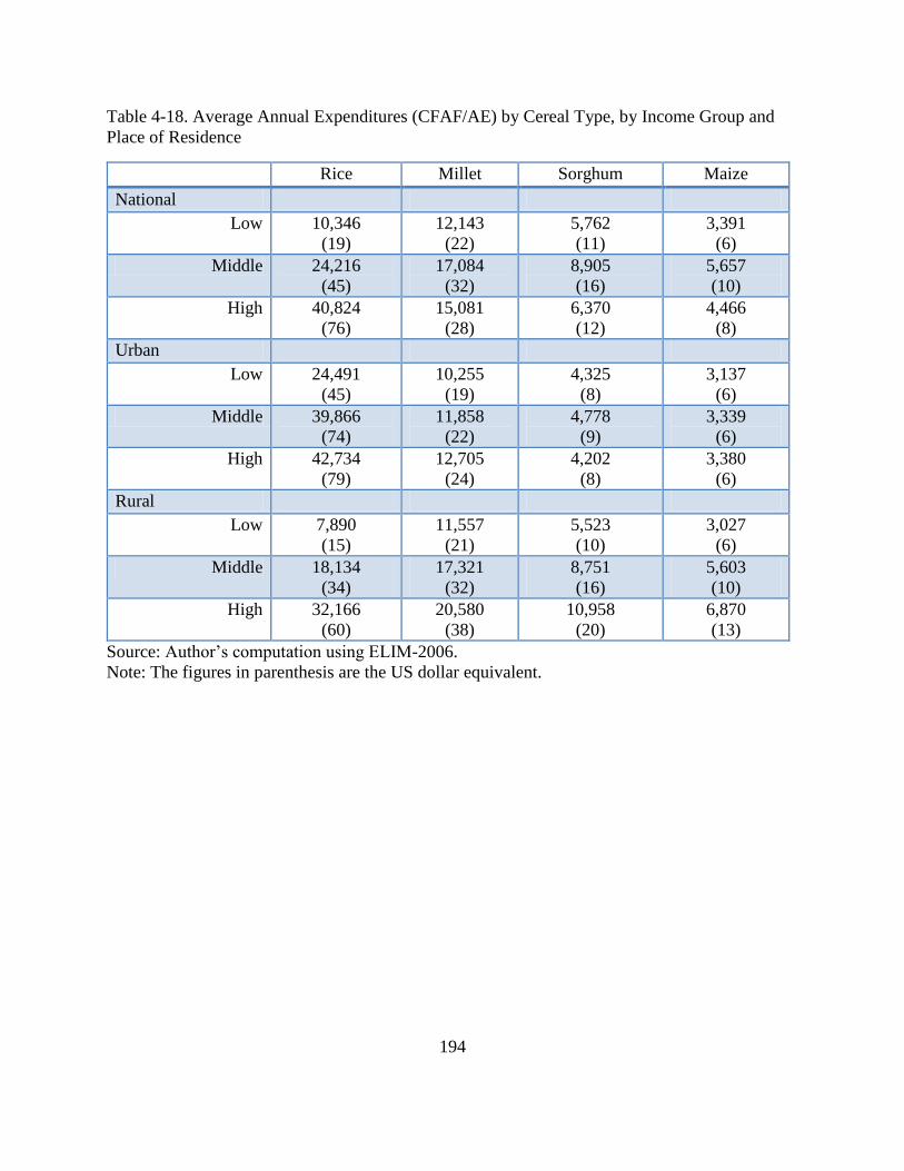
194
Table 4-18. Average Annual Expenditures (CFAF/AE) by Cereal Type, by Income Group and
Place of Residence
Rice Millet Sorghum Maize
National
Low 10,346
(19)
12,143
(22)
5,762
(11)
3,391
(6)
Middle 24,216
(45)
17,084
(32)
8,905
(16)
5,657
(10)
High 40,824
(76)
15,081
(28)
6,370
(12)
4,466
(8)
Urban
Low 24,491
(45)
10,255
(19)
4,325
(8)
3,137
(6)
Middle 39,866
(74)
11,858
(22)
4,778
(9)
3,339
(6)
High 42,734
(79)
12,705
(24)
4,202
(8)
3,380
(6)
Rural
Low 7,890
(15)
11,557
(21)
5,523
(10)
3,027
(6)
Middle 18,134
(34)
17,321
(32)
8,751
(16)
5,603
(10)
High 32,166
(60)
20,580
(38)
10,958
(20)
6,870
(13)
Source: Author’s computation using ELIM-2006.
Note: The figures in parenthesis are the US dollar equivalent.
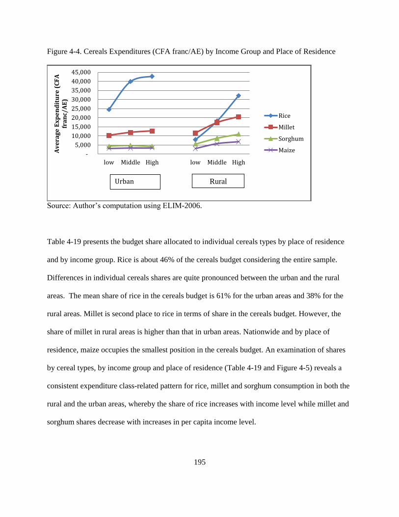
195
Figure 4-4. Cereals Expenditures (CFA franc/AE) by Income Group and Place of Residence
Source: Author’s computation using ELIM-2006.
Table 4-19 presents the budget share allocated to individual cereals types by place of residence
and by income group. Rice is about 46% of the cereals budget considering the entire sample.
Differences in individual cereals shares are quite pronounced between the urban and the rural
areas. The mean share of rice in the cereals budget is 61% for the urban areas and 38% for the
rural areas. Millet is second place to rice in terms of share in the cereals budget. However, the
share of millet in rural areas is higher than that in urban areas. Nationwide and by place of
residence, maize occupies the smallest position in the cereals budget. An examination of shares
by cereal types, by income group and place of residence (Table 4-19 and Figure 4-5) reveals a
consistent expenditure class-related pattern for rice, millet and sorghum consumption in both the
rural and the urban areas, whereby the share of rice increases with income level while millet and
sorghum shares decrease with increases in per capita income level.
-
5,000
10,000
15,000
20,000
25,000
30,000
35,000
40,000
45,000
low Middle High low Middle High
Av
era
ge
Ex
pe
nd
itu
re (
CF
A
fra
nc/
AE
)
Rice
Millet
Sorghum
Maize
Urban Rural
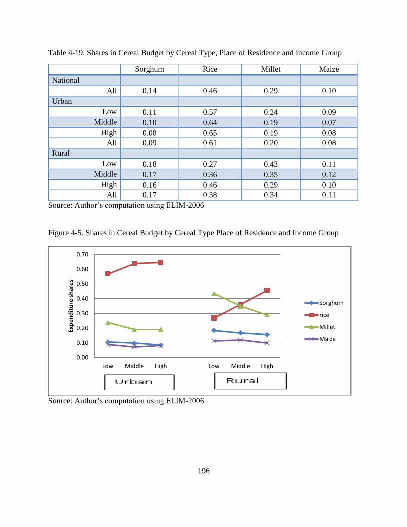
196
Table 4-19. Shares in Cereal Budget by Cereal Type, Place of Residence and Income Group
Sorghum Rice Millet Maize
National
All 0.14 0.46 0.29 0.10
Urban
Low 0.11 0.57 0.24 0.09
Middle 0.10 0.64 0.19 0.07
High 0.08 0.65 0.19 0.08
All 0.09 0.61 0.20 0.08
Rural
Low 0.18 0.27 0.43 0.11
Middle 0.17 0.36 0.35 0.12
High 0.16 0.46 0.29 0.10
All 0.17 0.38 0.34 0.11
Source: Author’s computation using ELIM-2006
Figure 4-5. Shares in Cereal Budget by Cereal Type Place of Residence and Income Group
Source: Author’s computation using ELIM-2006
0.00
0.10
0.20
0.30
0.40
0.50
0.60
0.70
Low Middle High Low Middle High
Exp
en
dit
ure
sh
are
s
Sorghum
rice
Millet
Maize
197
4.7.2. Household Cereals Demand: Econometric Results
Agricultural households are producers and consumers of food. Total output for agricultural
households is usually split between the household’s own-consumption and marketable surplus
(comprised of marketed surplus–the portion of production that is actually marketed—in
conjunction with gifts and in-kind exchanges). Several studies have been carried out to
understand how agricultural households make production and consumption decisions as well as
the allocation of household production to sales and home consumption. Based on different
assumptions, several arguments have been put forth on the responsiveness of own-consumption
and marketed surplus to market prices.
A key challenge is to estimate a complete demand system in a way consistent with the
microeconomic behavior of rural Malian agricultural households that captures these households
not only as food consumers, but also as food producers, operating under imperfect market
situations. The agricultural household model originally proposed by Singh et al., (1986) helps to
account for joint food consumption-production behavior, and the influence of influence of
production decision on consumption is captured through the “profit effect”. Yan and Chern
(2005), in the case of rural China, observed that production as well as market situations
(imperfect market in most developing countries) affect the consumption decision of an
agricultural household. As a result, they conclude that the marginal value of a food product
consumed is the sale price if there is a net sale for this food item; it is the purchase price if there
is a net purchase; and it is the shadow price if there is no purchase or sale.
As mentioned earlier, the estimation of a complete demand model that takes into account
how consumption decision is affected by production decision requires very detailed data which is
not available in this case. Furthermore, giving that the ELIM-2006 data set reports the value of
198
consumption (expenditure) on each commodity by mode of acquisition, it is very likely that
consumption from own-production was valued at market prices. Comparing aggregate
expenditure on cereals to the revenue from cereals sales, most households in the data set are
categorized as net cereals buyers. Thus, on the one hand, one could argue that amongst rural
Malian households the decision to purchase cereals as well as the amount of cereals to be
purchased is made conditional on the availability of cereals from own-production.
On the other hand, it can also be argued that a household’s consumption from own-
production does not go through the market and hence does not respond to market prices. Given
that cereals are major staples in the current context, it is hard to think of households selling
supplies from their own-production that were meant for household consumption due to high
market prices to buy other food items. However, households could also sell one type of cereal –
e.g., rice—and buy back a cheaper cereal, such as maize.
To examine both arguments, the estimation of cereals demand was first carried out using
total cereals expenditure (purchased and value of consumption from own production), and
second using only purchased cereals expenditures and aggregating expenditures across purchased
cereals . Although the results and discussions within this chapter focus on the first case, it makes
reference to the second case (parameters reported in the Appendix).
The estimation of household-level cereals demand involved three main steps. As
observed by Bopape (2006), the results of the test for model specification are influenced by
endogeneity in the total expenditure variable. Hence, the logical first step is to test for
endogeneity of cereals expenditure. Second, a formal test for model specification is performed
to determine the appropriateness of an AIDS or QUAIDS model. Third, the appropriate model is
estimated dealing with zero expenditure and expenditure endogeneity. Demand elasticities are
199
reported by income group and by place of residence in order to understand differences in
households’ cereals consumption behavior and any substitution between different cereal types.
A formal test for endogeneity in total cereals expenditures is conducted using the
augmented regression technique discussed earlier. The main challenge in the implementation of
the technique is the choice of instrument that must fulfill the relevance and the exogeneity
conditions of a good instrumental variable (IV). The relevance condition is that there must be
sufficient correlation between the instrument and the potentially endogenous variable, while the
exogeneity condition is that the instrument must not correlate with the error term in the demand
model. The number of wives to the household head is used as an IV here. This IV is expected to
be strongly correlated with total cereals expenditures in the sense that in Mali, the number of
wives to the household head (HH) is a measure of wealth and wealthier households are expected
to consume more cereals than households with fewer wives. The number of women in a
household could also influence consumption choices. However, the inclusion of household adult
equivalent as an additional explanatory variable in the demand model captures this additional
effect.
While the exogeneity condition of IVs is most often assumed, the relevance condition
must be tested. To formally test the relevance of the instrument, two reduced forms were
estimated–one for total cereals expenditure (lnCX) and the other for the square of total cereals
expenditures ((lnCX)2). In each reduced form, the number of wives to the HHH (nwife) and
nwife-squared were used as instruments. The estimated reduced forms with nwife and nwife
squared are reported in Table 4-20. The R-squared for the reduced form for lnCX is 0.210 while
that from the reduced form for (lnCX)2 is 0.2348. Following the estimation of the reduced forms,
a test for the relevance of the instruments was conducted. The test is a joint test for the statistical
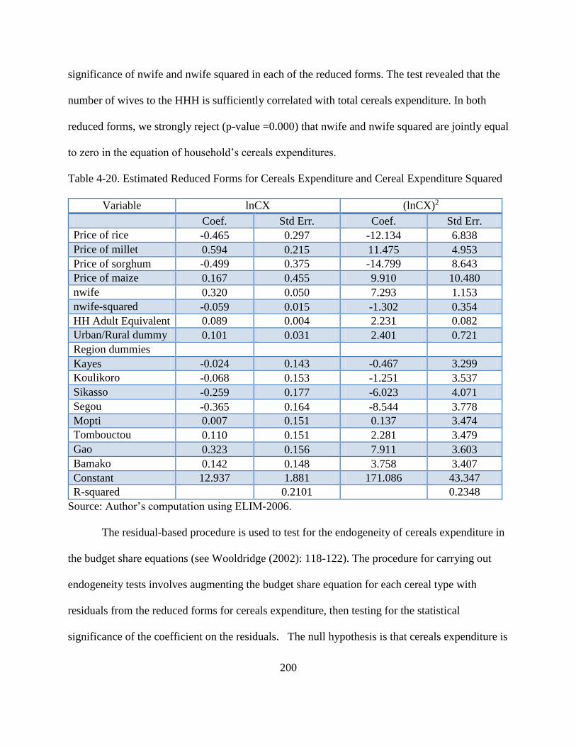
200
significance of nwife and nwife squared in each of the reduced forms. The test revealed that the
number of wives to the HHH is sufficiently correlated with total cereals expenditure. In both
reduced forms, we strongly reject (p-value =0.000) that nwife and nwife squared are jointly equal
to zero in the equation of household’s cereals expenditures.
Table 4-20. Estimated Reduced Forms for Cereals Expenditure and Cereal Expenditure Squared
Variable lnCX (lnCX)2
Coef. Std Err. Coef. Std Err.
Price of rice -0.465 0.297 -12.134 6.838
Price of millet 0.594 0.215 11.475 4.953
Price of sorghum -0.499 0.375 -14.799 8.643
Price of maize 0.167 0.455 9.910 10.480
nwife 0.320 0.050 7.293 1.153
nwife-squared -0.059 0.015 -1.302 0.354
HH Adult Equivalent 0.089 0.004 2.231 0.082
Urban/Rural dummy 0.101 0.031 2.401 0.721
Region dummies
Kayes -0.024 0.143 -0.467 3.299
Koulikoro -0.068 0.153 -1.251 3.537
Sikasso -0.259 0.177 -6.023 4.071
Segou -0.365 0.164 -8.544 3.778
Mopti 0.007 0.151 0.137 3.474
Tombouctou 0.110 0.151 2.281 3.479
Gao 0.323 0.156 7.911 3.603
Bamako 0.142 0.148 3.758 3.407
Constant 12.937 1.881 171.086 43.347
R-squared 0.2101 0.2348
Source: Author’s computation using ELIM-2006.
The residual-based procedure is used to test for the endogeneity of cereals expenditure in
the budget share equations (see Wooldridge (2002): 118-122). The procedure for carrying out
endogeneity tests involves augmenting the budget share equation for each cereal type with
residuals from the reduced forms for cereals expenditure, then testing for the statistical
significance of the coefficient on the residuals. The null hypothesis is that cereals expenditure is
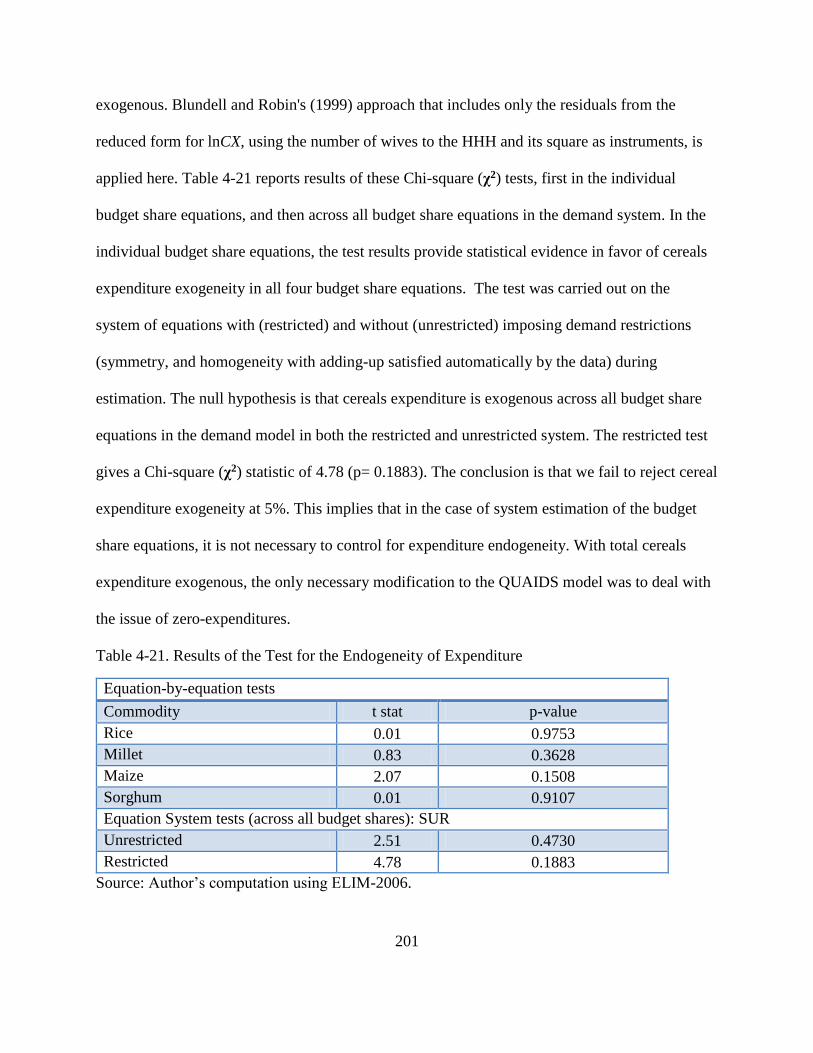
201
exogenous. Blundell and Robin's (1999) approach that includes only the residuals from the
reduced form for lnCX, using the number of wives to the HHH and its square as instruments, is
applied here. Table 4-21 reports results of these Chi-square (χ2) tests, first in the individual
budget share equations, and then across all budget share equations in the demand system. In the
individual budget share equations, the test results provide statistical evidence in favor of cereals
expenditure exogeneity in all four budget share equations. The test was carried out on the
system of equations with (restricted) and without (unrestricted) imposing demand restrictions
(symmetry, and homogeneity with adding-up satisfied automatically by the data) during
estimation. The null hypothesis is that cereals expenditure is exogenous across all budget share
equations in the demand model in both the restricted and unrestricted system. The restricted test
gives a Chi-square (χ2) statistic of 4.78 (p= 0.1883). The conclusion is that we fail to reject cereal
expenditure exogeneity at 5%. This implies that in the case of system estimation of the budget
share equations, it is not necessary to control for expenditure endogeneity. With total cereals
expenditure exogenous, the only necessary modification to the QUAIDS model was to deal with
the issue of zero-expenditures.
Table 4-21. Results of the Test for the Endogeneity of Expenditure
Equation-by-equation tests
Commodity t stat p-value
Rice 0.01 0.9753
Millet 0.83 0.3628
Maize 2.07 0.1508
Sorghum 0.01 0.9107
Equation System tests (across all budget shares): SUR
Unrestricted 2.51 0.4730
Restricted 4.78 0.1883
Source: Author’s computation using ELIM-2006.
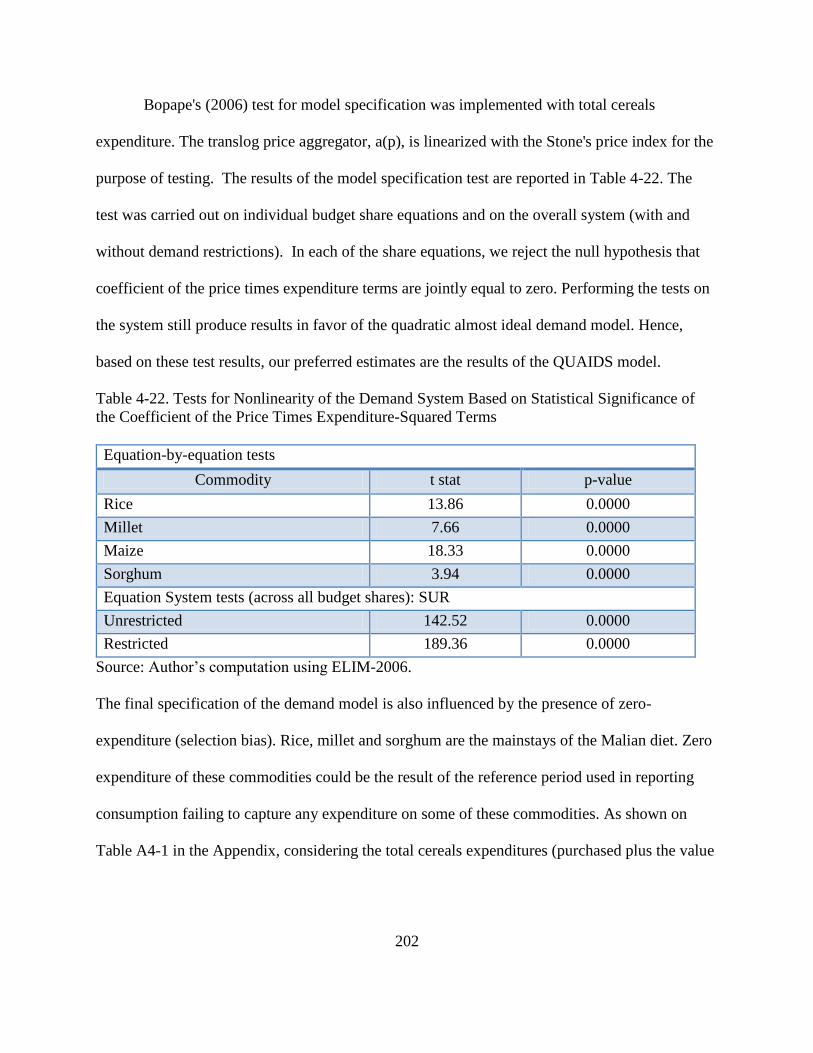
202
Bopape's (2006) test for model specification was implemented with total cereals
expenditure. The translog price aggregator, a(p), is linearized with the Stone's price index for the
purpose of testing. The results of the model specification test are reported in Table 4-22. The
test was carried out on individual budget share equations and on the overall system (with and
without demand restrictions). In each of the share equations, we reject the null hypothesis that
coefficient of the price times expenditure terms are jointly equal to zero. Performing the tests on
the system still produce results in favor of the quadratic almost ideal demand model. Hence,
based on these test results, our preferred estimates are the results of the QUAIDS model.
Table 4-22. Tests for Nonlinearity of the Demand System Based on Statistical Significance of
the Coefficient of the Price Times Expenditure-Squared Terms
Equation-by-equation tests
Commodity t stat p-value
Rice 13.86 0.0000
Millet 7.66 0.0000
Maize 18.33 0.0000
Sorghum 3.94 0.0000
Equation System tests (across all budget shares): SUR
Unrestricted 142.52 0.0000
Restricted 189.36 0.0000
Source: Author’s computation using ELIM-2006.
The final specification of the demand model is also influenced by the presence of zero-
expenditure (selection bias). Rice, millet and sorghum are the mainstays of the Malian diet. Zero
expenditure of these commodities could be the result of the reference period used in reporting
consumption failing to capture any expenditure on some of these commodities. As shown on
Table A4-1 in the Appendix, considering the total cereals expenditures (purchased plus the value
203
of own-consumption)37, 5.1% of the total sample reported zero expenditure on rice, 45.2%
reported zero expenditure on sorghum, 18.9% reported zero expenditure on millet and 49.8%
reported zero expenditure on maize. Therefore, to check if any fundamental difference exists
between the decisions to purchase these cereals and how much of each to purchase, the QUAIDS
model for cereals demand is estimated dealing with zero-expenditure (censored).
The general procedure in the estimation of the censored QUAIDS model in the absence of
any expenditure endogeneity is as follows: we estimate the household’s decision to consume a
specific cereal type (Equation 4-3) by using a maximum likelihood probit regression to obtain
household-specific probit estimates σ̂hzih. The univariate standard normal probability density (pdf)
and the cumulative distribution (cdf) to use in the QUAIDS model are later calculated for each
cereal type and each household. Given the initial values of the price index a(p) and the predicted
values (pdfs and cdfs) from the probit regressions, the cross-equation nature of the restrictions,
and the non-linear structure of the QUAIDS model, Poi’s (2008) “demand-system estimation:
update, Non-Linear Seemingly Unrelated regression (NLSUR) model” written in STATA,
augmented with the pdf and cdf from the first stage probit regression to account for zero
expenditure and household demographics, is used to estimate the demand system in equation 4-5
( dropping the term 𝜌𝑠𝜏𝑠𝑖 since we rejected expenditure endogeneity).
37 Disaggregating zero expenditures by mode of acquisition, it is observed that 27% of the
households purchased sorghum in the reference period, 80% had positive purchases for rice, 51%
purchased millet and 19% purchased maize in the reference period. For rice for instance, the
percentage zero expenditure drops from 20% (considering only purchased cereals expenditures)
to 5.1% (considering total cereals expenditures (purchased plus value of own consumption) in
the reference period. Thus, some households may not have purchased rice but they consumed
rice from their own production.
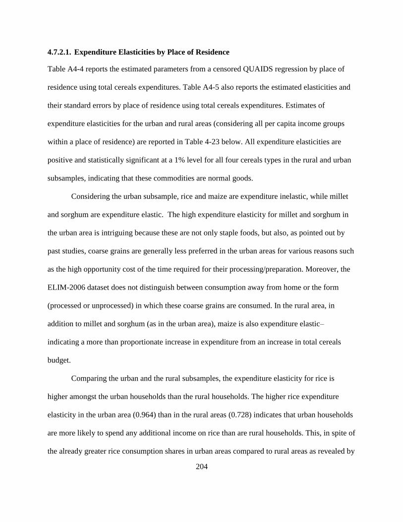
204
4.7.2.1. Expenditure Elasticities by Place of Residence
Table A4-4 reports the estimated parameters from a censored QUAIDS regression by place of
residence using total cereals expenditures. Table A4-5 also reports the estimated elasticities and
their standard errors by place of residence using total cereals expenditures. Estimates of
expenditure elasticities for the urban and rural areas (considering all per capita income groups
within a place of residence) are reported in Table 4-23 below. All expenditure elasticities are
positive and statistically significant at a 1% level for all four cereals types in the rural and urban
subsamples, indicating that these commodities are normal goods.
Considering the urban subsample, rice and maize are expenditure inelastic, while millet
and sorghum are expenditure elastic. The high expenditure elasticity for millet and sorghum in
the urban area is intriguing because these are not only staple foods, but also, as pointed out by
past studies, coarse grains are generally less preferred in the urban areas for various reasons such
as the high opportunity cost of the time required for their processing/preparation. Moreover, the
ELIM-2006 dataset does not distinguish between consumption away from home or the form
(processed or unprocessed) in which these coarse grains are consumed. In the rural area, in
addition to millet and sorghum (as in the urban area), maize is also expenditure elastic–
indicating a more than proportionate increase in expenditure from an increase in total cereals
budget.
Comparing the urban and the rural subsamples, the expenditure elasticity for rice is
higher amongst the urban households than the rural households. The higher rice expenditure
elasticity in the urban area (0.964) than in the rural areas (0.728) indicates that urban households
are more likely to spend any additional income on rice than are rural households. This, in spite of
the already greater rice consumption shares in urban areas compared to rural areas as revealed by
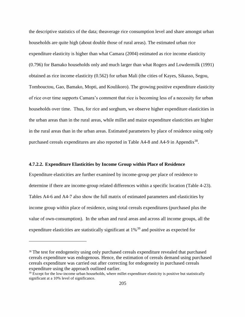
205
the descriptive statistics of the data; theaverage rice consumption level and share amongst urban
households are quite high (about double those of rural areas). The estimated urban rice
expenditure elasticity is higher than what Camara (2004) estimated as rice income elasticity
(0.796) for Bamako households only and much larger than what Rogers and Lowdermilk (1991)
obtained as rice income elasticity (0.562) for urban Mali (the cities of Kayes, Sikasso, Segou,
Tombouctou, Gao, Bamako, Mopti, and Koulikoro). The growing positive expenditure elasticity
of rice over time supports Camara’s comment that rice is becoming less of a necessity for urban
households over time. Thus, for rice and sorghum, we observe higher expenditure elasticities in
the urban areas than in the rural areas, while millet and maize expenditure elasticities are higher
in the rural areas than in the urban areas. Estimated parameters by place of residence using only
purchased cereals expenditures are also reported in Table A4-8 and A4-9 in Appendix38.
4.7.2.2. Expenditure Elasticities by Income Group within Place of Residence
Expenditure elasticities are further examined by income-group per place of residence to
determine if there are income-group related differences within a specific location (Table 4-23).
Tables A4-6 and A4-7 also show the full matrix of estimated parameters and elasticities by
income group within place of residence, using total cereals expenditures (purchased plus the
value of own-consumption). In the urban and rural areas and across all income groups, all the
expenditure elasticities are statistically significant at 1%39 and positive as expected for
38 The test for endogeneity using only purchased cereals expenditure revealed that purchased
cereals expenditure was endogenous. Hence, the estimation of cereals demand using purchased
cereals expenditure was carried out after correcting for endogeneity in purchased cereals
expenditure using the approach outlined earlier. 39 Except for the low-income urban households, where millet expenditure elasticity is positive but statistically
significant at a 10% level of significance.
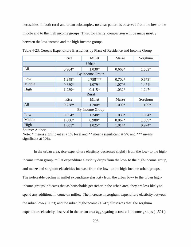
206
necessities. In both rural and urban subsamples, no clear pattern is observed from the low to the
middle and to the high income groups. Thus, for clarity, comparison will be made mostly
between the low-income and the high-income groups.
Table 4-23. Cereals Expenditure Elasticities by Place of Residence and Income Group
Rice Millet Maize Sorghum
Urban
All 0.964* 1.038* 0.668* 1.502*
By Income Group
Low 1.248* 0.758*** 0.702* 0.673*
Middle 0.880* 1.079* 1.070* 1.454*
High 1.239* 0.415* 1.032* 1.247*
Rural
Rice Millet Maize Sorghum
All 0.728* 1.200* 1.099* 1.109*
By Income Group
Low 0.654* 1.248* 1.030* 1.054*
Middle 1.006* 0.980* 0.867* 1.069*
High 1.001* 1.025* 1.014* 0.974*
Source: Author.
Note: * means significant at a 1% level and ** means significant at 5% and *** means
significant at 10%.
In the urban area, rice expenditure elasticity decreases slightly from the low- to the high-
income urban group, millet expenditure elasticity drops from the low- to the high-income group,
and maize and sorghum elasticities increase from the low- to the high-income urban groups.
The noticeable decline in millet expenditure elasticity from the urban low- to the urban high-
income groups indicates that as households get richer in the urban area, they are less likely to
spend any additional income on millet. The increase in sorghum expenditure elasticity between
the urban low- (0.673) and the urban high-income (1.247) illustrates that the sorghum
expenditure elasticity observed in the urban area aggregating across all income groups (1.501 )
207
is largely driven by the behavior of the urban middle- and high-income groups. Hence, in terms
of expenditure elasticities, in the urban area, we observe a high preference for rice and sorghum
at higher per capita income levels while the preference for millet seems to decrease with income
level. The high expenditure of elasticity of sorghum as income increases calls for attention and
warrants further investigation into the type or form in which sorghum is consumed in the urban
area. There is a need to differentiate demand for sorghum of different quality (processed and
unprocessed) and by place of consumption (for example, home and away from home).
Rural households also reveal high expenditure elasticities across all income groups for all
the different cereals when total cereals expenditures are used. The responsiveness of rice to
changes in income increases from the low- to the high-income households. Millet, sorghum and
to a lesser extent maize expenditure elasticities tend to decline from the rural low- to the high-
income rural group.
Overall, using total cereals expenditures, the hypothesis that poorer households have
higher expenditure elasticities is true for millet, sorghum and to a lesser extent maize in the rural
areas and millet in the urban areas. From the summary statistics (Table 4-19), we observe a clear
pattern of decline in sorghum and millet budget shares from the low- to the high-income groups
and a marked increase in the rice budget share from the rural low- to high-income households.
Expenditure elasticities by income group and place of residence estimated using only purchased
cereals expenditures are also reported in Tables A4-10 and A4-11.
4.7.2.3. Own-Price Responses by Place of Residence
Table 4-24 reports uncompensated and compensated own-price elasticities of cereals demand by
place of residence using total cereals expenditures (purchased plus value of own-consumption).
208
Table A4-5 in Appendix also reports the standard errors of the estimated elasticities. All
uncompensated and compensated own-price elasticities are not only statistically significant at a
5% level, but are also negative in both the urban and the rural sub-samples, thus supporting a
downward sloping demand curve.
Considering the urban area (without disaggregating by income group), all uncompensated
own-price elasticities are close to unity, indicating high sensitivity to own price changes. The
own-price elasticity for rice obtained here for the urban area (-0.955) are about 3 times that
reported by Camara (2004) using data for Bamako households only (-0.338). However, Rogers
and Lowdermilk (1991) using urban Malian data found the own-price elasticity of demand for
rice to be -0.683. Given that the urban sample used by Rogers and Lowdermilk (1991) is quite
comparable to that used in this study (in terms of geographical coverage), it can be noted that the
sensitivity of rice demand to changes in its own-price in the urban areas appears to have
increased over two decades. When the substitution effects are considered, all the cereals became
less elastic, as the urban compensated own-price elasticities get smaller in magnitude than
uncompensated own-price elasticities, as expected for normal goods. Considering total cereals
expenditures, millet demand is the least sensitive to changes in its own price in the urban area.
Thus, the hypothesis that rice is the least responsive to changes in its own price in the urban area
due to the high opportunity cost of time and demand for convenience by urban time-poor
consumers is rejected. Notwithstanding, compared to maize and sorghum, rice demand is less
responsive to changes in its own price.
Still using total cereals expenditures and without disaggregating by income group, in the
rural area, all statistically significant uncompensated own-price elasticities are negative as
expected. Rice is the least sensitive to changes in its own price in the rural area. The estimated
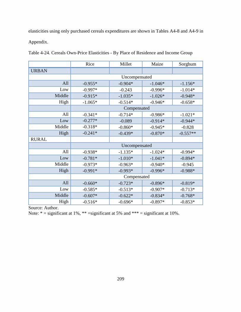
209
elasticities using only purchased cereals expenditures are shown in Tables A4-8 and A4-9 in
Appendix.
Table 4-24. Cereals Own-Price Elasticities - By Place of Residence and Income Group
Rice Millet Maize Sorghum
URBAN
Uncompensated
All -0.955* -0.904* -1.046* -1.156*
Low -0.997* -0.243 -0.996* -1.014*
Middle -0.915* -1.035* -1.026* -0.948*
High -1.065* -0.514* -0.946* -0.658*
Compensated
All -0.341* -0.714* -0.986* -1.021*
Low -0.277* -0.089 -0.914* -0.944*
Middle -0.318* -0.860* -0.945* -0.828
High -0.241* -0.439* -0.870* -0.557**
RURAL
Uncompensated
All -0.938* -1.135* -1.024* -0.994*
Low -0.781* -1.010* -1.041* -0.894*
Middle -0.973* -0.963* -0.940* -0.945
High -0.991* -0.993* -0.996* -0.988*
Compensated
All -0.660* -0.723* -0.896* -0.819*
Low -0.585* -0.513* -0.907* -0.713*
Middle -0.607* -0.622* -0.834* -0.768*
High -0.516* -0.696* -0.897* -0.853*
Source: Author.
Note: * = significant at 1%, ** =significant at 5% and *** = significant at 10%.
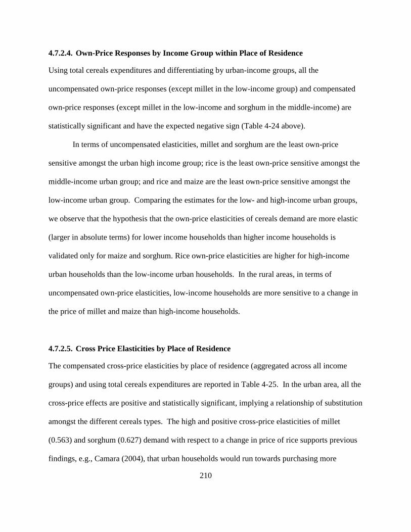
210
4.7.2.4. Own-Price Responses by Income Group within Place of Residence
Using total cereals expenditures and differentiating by urban-income groups, all the
uncompensated own-price responses (except millet in the low-income group) and compensated
own-price responses (except millet in the low-income and sorghum in the middle-income) are
statistically significant and have the expected negative sign (Table 4-24 above).
In terms of uncompensated elasticities, millet and sorghum are the least own-price
sensitive amongst the urban high income group; rice is the least own-price sensitive amongst the
middle-income urban group; and rice and maize are the least own-price sensitive amongst the
low-income urban group. Comparing the estimates for the low- and high-income urban groups,
we observe that the hypothesis that the own-price elasticities of cereals demand are more elastic
(larger in absolute terms) for lower income households than higher income households is
validated only for maize and sorghum. Rice own-price elasticities are higher for high-income
urban households than the low-income urban households. In the rural areas, in terms of
uncompensated own-price elasticities, low-income households are more sensitive to a change in
the price of millet and maize than high-income households.
4.7.2.5. Cross Price Elasticities by Place of Residence
The compensated cross-price elasticities by place of residence (aggregated across all income
groups) and using total cereals expenditures are reported in Table 4-25. In the urban area, all the
cross-price effects are positive and statistically significant, implying a relationship of substitution
amongst the different cereals types. The high and positive cross-price elasticities of millet
(0.563) and sorghum (0.627) demand with respect to a change in price of rice supports previous
findings, e.g., Camara (2004), that urban households would run towards purchasing more
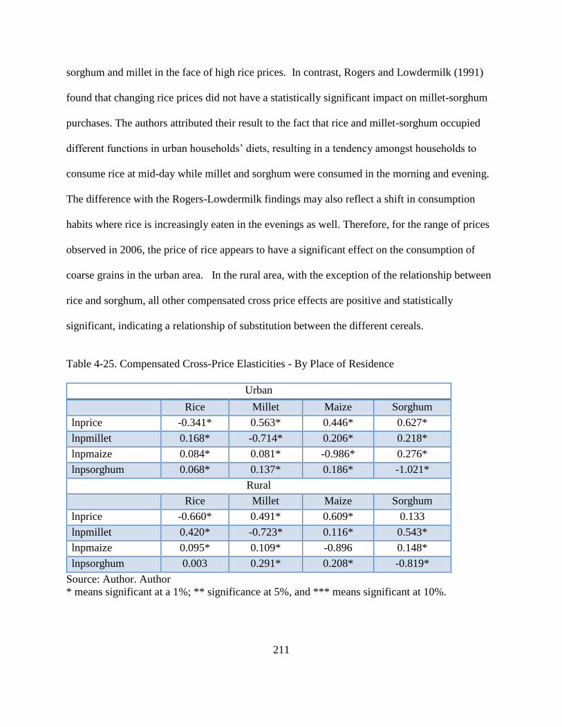
211
sorghum and millet in the face of high rice prices. In contrast, Rogers and Lowdermilk (1991)
found that changing rice prices did not have a statistically significant impact on millet-sorghum
purchases. The authors attributed their result to the fact that rice and millet-sorghum occupied
different functions in urban households’ diets, resulting in a tendency amongst households to
consume rice at mid-day while millet and sorghum were consumed in the morning and evening.
The difference with the Rogers-Lowdermilk findings may also reflect a shift in consumption
habits where rice is increasingly eaten in the evenings as well. Therefore, for the range of prices
observed in 2006, the price of rice appears to have a significant effect on the consumption of
coarse grains in the urban area. In the rural area, with the exception of the relationship between
rice and sorghum, all other compensated cross price effects are positive and statistically
significant, indicating a relationship of substitution between the different cereals.
Table 4-25. Compensated Cross-Price Elasticities - By Place of Residence
Urban
Rice Millet Maize Sorghum
lnprice -0.341* 0.563* 0.446* 0.627*
lnpmillet 0.168* -0.714* 0.206* 0.218*
lnpmaize 0.084* 0.081* -0.986* 0.276*
lnpsorghum 0.068* 0.137* 0.186* -1.021*
Rural
Rice Millet Maize Sorghum
lnprice -0.660* 0.491* 0.609* 0.133
lnpmillet 0.420* -0.723* 0.116* 0.543*
lnpmaize 0.095* 0.109* -0.896 0.148*
lnpsorghum 0.003 0.291* 0.208* -0.819*
Source: Author. Author
* means significant at a 1%; ** significance at 5%, and *** means significant at 10%.
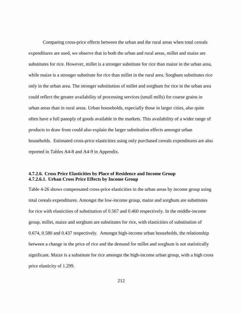
212
Comparing cross-price effects between the urban and the rural areas when total cereals
expenditures are used, we observe that in both the urban and rural areas, millet and maize are
substitutes for rice. However, millet is a stronger substitute for rice than maize in the urban area,
while maize is a stronger substitute for rice than millet in the rural area. Sorghum substitutes rice
only in the urban area. The stronger substitution of millet and sorghum for rice in the urban area
could reflect the greater availability of processing services (small mills) for coarse grains in
urban areas than in rural areas. Urban households, especially those in larger cities, also quite
often have a full panoply of goods available in the markets. This availability of a wider range of
products to draw from could also explain the larger substitution effects amongst urban
households. Estimated cross-price elasticities using only purchased cereals expenditures are also
reported in Tables A4-8 and A4-9 in Appendix.
4.7.2.6. Cross Price Elasticities by Place of Residence and Income Group
4.7.2.6.1. Urban Cross Price Effects by Income Group
Table 4-26 shows compensated cross-price elasticities in the urban areas by income group using
total cereals expenditures. Amongst the low-income group, maize and sorghum are substitutes
for rice with elasticities of substitution of 0.567 and 0.460 respectively. In the middle-income
group, millet, maize and sorghum are substitutes for rice, with elasticities of substitution of
0.674, 0.580 and 0.437 respectively. Amongst high-income urban households, the relationship
between a change in the price of rice and the demand for millet and sorghum is not statistically
significant. Maize is a substitute for rice amongst the high-income urban group, with a high cross
price elasticity of 1.299.
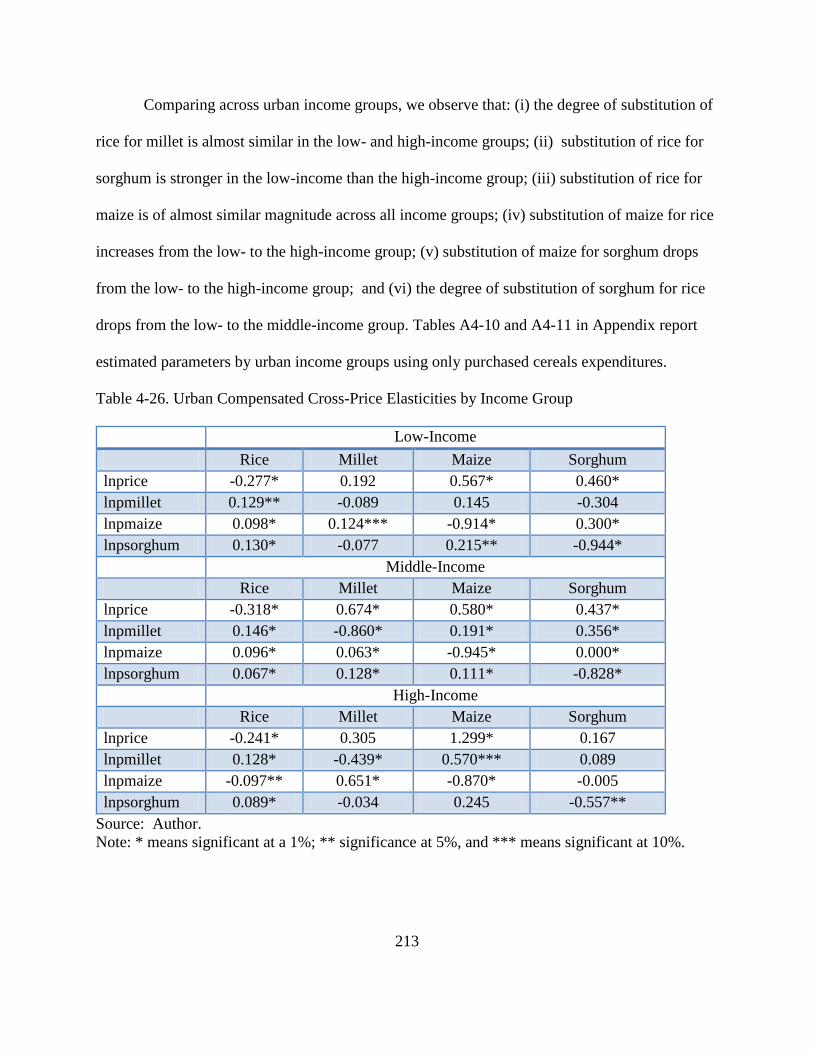
213
Comparing across urban income groups, we observe that: (i) the degree of substitution of
rice for millet is almost similar in the low- and high-income groups; (ii) substitution of rice for
sorghum is stronger in the low-income than the high-income group; (iii) substitution of rice for
maize is of almost similar magnitude across all income groups; (iv) substitution of maize for rice
increases from the low- to the high-income group; (v) substitution of maize for sorghum drops
from the low- to the high-income group; and (vi) the degree of substitution of sorghum for rice
drops from the low- to the middle-income group. Tables A4-10 and A4-11 in Appendix report
estimated parameters by urban income groups using only purchased cereals expenditures.
Table 4-26. Urban Compensated Cross-Price Elasticities by Income Group
Low-Income
Rice Millet Maize Sorghum
lnprice -0.277* 0.192 0.567* 0.460*
lnpmillet 0.129** -0.089 0.145 -0.304
lnpmaize 0.098* 0.124*** -0.914* 0.300*
lnpsorghum 0.130* -0.077 0.215** -0.944*
Middle-Income
Rice Millet Maize Sorghum
lnprice -0.318* 0.674* 0.580* 0.437*
lnpmillet 0.146* -0.860* 0.191* 0.356*
lnpmaize 0.096* 0.063* -0.945* 0.000*
lnpsorghum 0.067* 0.128* 0.111* -0.828*
High-Income
Rice Millet Maize Sorghum
lnprice -0.241* 0.305 1.299* 0.167
lnpmillet 0.128* -0.439* 0.570*** 0.089
lnpmaize -0.097** 0.651* -0.870* -0.005
lnpsorghum 0.089* -0.034 0.245 -0.557**
Source: Author.
Note: * means significant at a 1%; ** significance at 5%, and *** means significant at 10%.
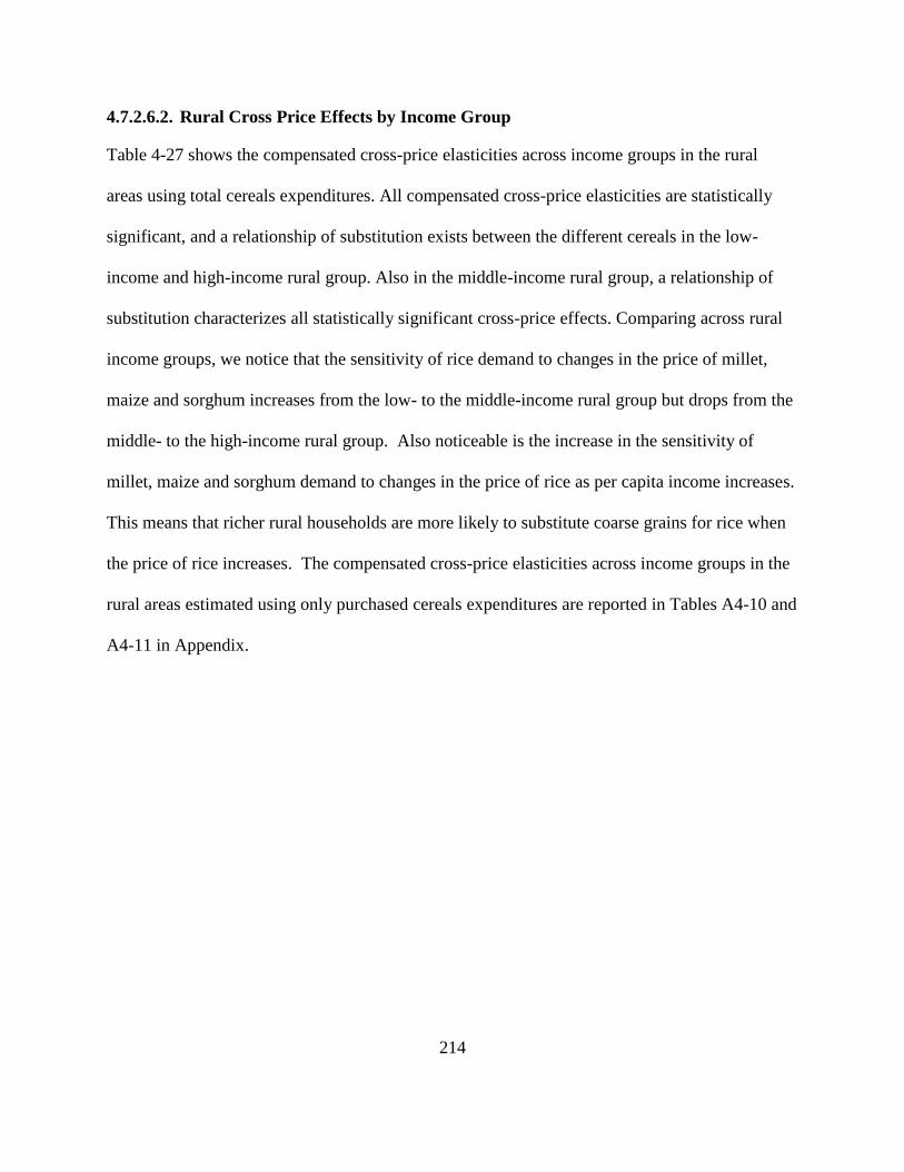
214
4.7.2.6.2. Rural Cross Price Effects by Income Group
Table 4-27 shows the compensated cross-price elasticities across income groups in the rural
areas using total cereals expenditures. All compensated cross-price elasticities are statistically
significant, and a relationship of substitution exists between the different cereals in the low-
income and high-income rural group. Also in the middle-income rural group, a relationship of
substitution characterizes all statistically significant cross-price effects. Comparing across rural
income groups, we notice that the sensitivity of rice demand to changes in the price of millet,
maize and sorghum increases from the low- to the middle-income rural group but drops from the
middle- to the high-income rural group. Also noticeable is the increase in the sensitivity of
millet, maize and sorghum demand to changes in the price of rice as per capita income increases.
This means that richer rural households are more likely to substitute coarse grains for rice when
the price of rice increases. The compensated cross-price elasticities across income groups in the
rural areas estimated using only purchased cereals expenditures are reported in Tables A4-10 and
A4-11 in Appendix.
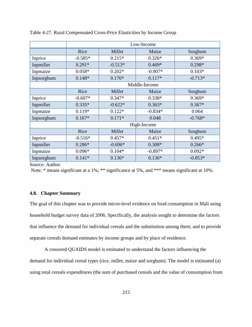
215
Table 4-27. Rural Compensated Cross-Price Elasticities by Income Group
Low-Income
Rice Millet Maize Sorghum
lnprice -0.585* 0.215* 0.326* 0.369*
lnpmillet 0.291* -0.513* 0.469* 0.298*
lnpmaize 0.058* 0.202* -0.907* 0.103*
lnpsorghum 0.148* 0.176* 0.117* -0.713*
Middle-Income
Rice Millet Maize Sorghum
lnprice -0.607* 0.347* 0.338* 0.369*
lnpmillet 0.335* -0.622* 0.363* 0.367*
lnpmaize 0.119* 0.122* -0.834* 0.064
lnpsorghum 0.167* 0.171* 0.048 -0.768*
High-Income
Rice Millet Maize Sorghum
lnprice -0.516* 0.457* 0.451* 0.495*
lnpmillet 0.286* -0.696* 0.308* 0.266*
lnpmaize 0.096* 0.104* -0.897* 0.092*
lnpsorghum 0.141* 0.136* 0.136* -0.853*
Source: Author.
Note: * means significant at a 1%; ** significance at 5%, and *** means significant at 10%.
4.8. Chapter Summary
The goal of this chapter was to provide micro-level evidence on food consumption in Mali using
household budget survey data of 2006. Specifically, the analysis sought to determine the factors
that influence the demand for individual cereals and the substitution among them; and to provide
separate cereals demand estimates by income groups and by place of residence.
A censored QUAIDS model is estimated to understand the factors influencing the
demand for individual cereal types (rice, millet, maize and sorghum). The model is estimated (a)
using total cereals expenditures (the sum of purchased cereals and the value of consumption from

216
own-production), and (b) using only purchased cereals expenditures. The estimated parameters
under scenario (b) are reported in the appendix.
Positive expenditure elasticities were found for all four cereals type, irrespective of place
of residence. Using total cereals expenditure, rice and sorghum expenditure elasticities were
found to be higher in the urban area than in the rural areas, while millet and maize expenditure
elasticities are higher in the rural areas than in the urban areas. Comparing rice expenditure
elasticity estimated for the urban area in this study to that reported by previous studies in Mali
(e.g., Camara, 2004), we observe a positive trend over time and find support for Camara’s
assertion that rice is becoming less of a necessity for urban households over time. The high
expenditure elasticity of sorghum in the urban area calls for further investigations into the quality
of sorghum that is consumed, since it is often argued that coarse grains (such as sorghum) are
more time consuming and less convenient for urban time poor consumers.
The analysis of expenditure elasticities by income-group and place of residence also
reveals some income group-related pattern for rice and millet and to a lesser extent sorghum in
the urban area. Using total cereals expenditures, we observe in the urban area a high preference
for rice and sorghum at higher per capita income levels while the preference for millet seems to
decrease with income level. The high expenditure elasticity of sorghum as income increases
indicates a need to differentiate sorghum demand by quality (processed and unprocessed) and by
place of consumption (for example, home and away from home). While the expenditure
elasticity for millet decreases with increases income amongst urban households, amongst rural
households, millet, sorghum and to a lesser extent maize expenditure elasticities tend to decline
from the rural low- to the high-income households. This suggests declining preference for
coarse grains as rural households get richer.
217
Uncompensated and compensated own-price elasticities by place of residence support a
downward-sloping demand curve for all cereals. Considering total cereals expenditures and
without disaggregating by income groups, the hypothesis that rice is the least responsive to
changes in its own price in the urban area due to the high opportunity cost of time and demand
for convenience by urban-poor consumers is rejected. Millet is the least sensitive to changes in
its own price in the urban areas. Rice is the least sensitive to changes in its own price in the rural
area.
The analysis of own-price elasticities by income group and place of residence using total
cereals expenditures reveal that amongst urban households, only maize and sorghum support the
hypothesis that the own-price elasticities of cereals demand are more elastic (larger in absolute
terms) for lower income households than higher income households. High-income urban
households were found to have higher own-price elasticities for rice than the low-income urban
households. In the rural areas, low-income households were more sensitive to a change in the
price of millet and maize than high-income households.
The analysis also reveals that a relationship of substitution characterizes most statistically
significant cross-price effects. Using total cereals expenditures and aggregating all income
groups, in the urban areas we observe high and positive cross-price elasticities of millet and
sorghum demand with respect to a change in the price of rice. This finding supports previous
findings (e.g., Camara, 2004), that urban households would run towards purchasing more
sorghum and millet in the face of high rice prices. Compensated cross-price elasticities in the
rural areas also indicate a relationship of substitution between the different cereals.
Furthermore, comparing the urban and the rural areas in terms of the magnitude of cross-
price effects, we observe a stronger substitution of millet and sorghum for rice amongst urban
218
households. This could reflect the greater availability of processing services (small mills) for
coarse grains in urban areas, as well as the fact that urban markets, especially in larger cities, also
quite often make a wider range of products available to consumers.
Compensated cross-price elasticities by income group in the urban area using total cereals
expenditures reveal that amongst urban households, while the degree of substitution of rice for
millet is almost similar in the low- and high-income groups, the degree of substitution of rice for
sorghum is stronger in the low-income than the high-income group. The substitution of maize for
rice increases from the low- to the high-income group, while the substitution of maize for
sorghum drops from the low- to the high-income group.
Comparing across rural income groups and using total cereals expenditures, we notice an
increase in the sensitivity of millet, maize and sorghum demand to changes in the price of rice as
per capita income increases. This means that richer rural households are more likely to substitute
coarse grains for rice when the price of rice increases.
The preceding analysis reveals high substitution between rice and coarse grains in both
the rural and the urban areas and across income groups. This finding implies some scope for
dealing with price spikes for one cereal by increasing the availability of substitutes—a possibility
that the earlier findings of low cross-elasticities seemed to discount.

219
APPENDIX
220
Table A4-1. Structure of ELIM-2006 data
Region Cercle Arrondissement Market with available prices
1. KAYES 1. Kayes Kayes central
Ambidedi
Aourou
Diamou
Sadiola
Same
Segala
Kayes
Kayes Centre
KayesN'Dy
Kayes Plateau
2. Bafoulab
é
Bafoulabe central
Bamafele
Diakon
Goundara
Koundian
Mahina
Bafoulabe central
Bamafele
Diakon
Goundara
3. Diéma Diema central Diéma
Bema
Diangountecamar
Dioumara
Lakamane
4. Kéniéba Kenieba central
Faraba
5. Kita Kita central
Djidian
Kokofata
Sebekoro Badinko
Sefeto
Sirakoro
Toukoto
Kita Kita
6. Nioro Nioro central
Gavinane
Simbi
Troungoumbe
Nioro Nioro
7. Yélimané Yelimane central
Kirane
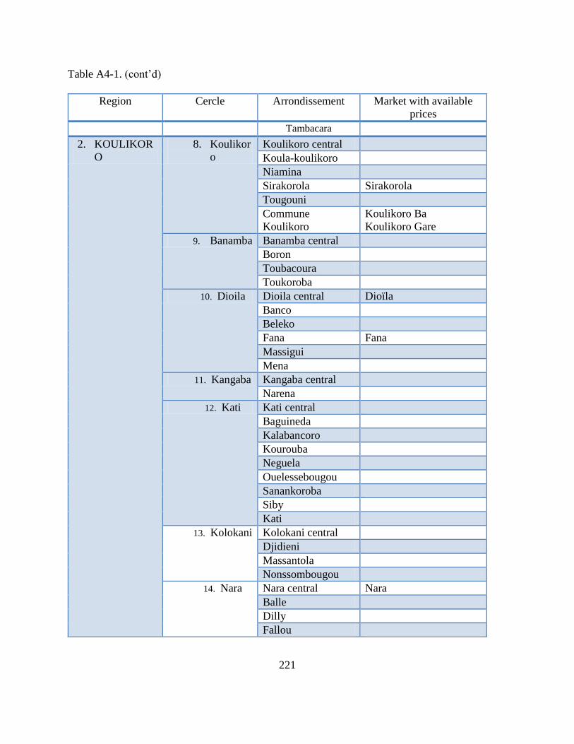
221
Table A4-1. (cont’d)
Region Cercle Arrondissement Market with available
prices
Tambacara
2. KOULIKOR
O
8. Koulikor
o
Koulikoro central
Koula-koulikoro
Niamina
Sirakorola Sirakorola
Tougouni
Commune
Koulikoro
Koulikoro Ba
Koulikoro Gare
9. Banamba Banamba central
Boron
Toubacoura
Toukoroba
10. Dioila Dioila central Dioïla
Banco
Beleko
Fana Fana
Massigui
Mena
11. Kangaba Kangaba central
Narena
12. Kati Kati central
Baguineda
Kalabancoro
Kourouba
Neguela
Ouelessebougou
Sanankoroba
Siby
Kati
13. Kolokani Kolokani central
Djidieni
Massantola
Nonssombougou
14. Nara Nara central Nara
Balle
Dilly
Fallou
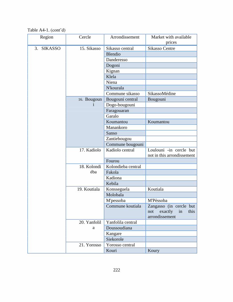
222
Table A4-1. (cont’d)
Region Cercle Arrondissement Market with available
prices
3. SIKASSO 15. Sikasso Sikasso central Sikasso Centre
Blendio
Danderesso
Dogoni
Kignan
Klela
Niena
N'kourala
Commune sikasso SikassoMédine
16. Bougoun
i
Bougouni central Bougouni
Dogo-bougouni
Faragouaran
Garalo
Koumantou Koumantou
Manankoro
Sanso
Zantiebougou
Commune bougouni
17. Kadiolo Kadiolo central Loulouni -in cercle but
not in this arrondissement
Fourou
18. Kolondi
éba
Kolondieba central
Fakola
Kadiona
Kebila
19. Koutiala Konsseguela Koutiala
Molobala
M'pessoba M'Pèssoba
Commune koutiala Zangasso (in cercle but
not exactly in this
arrondissement
20. Yanfolil
a
Yanfolila central
Doussoudiana
Kangare
Siekorole
21. Yorosso Yorosso central
Kouri Koury
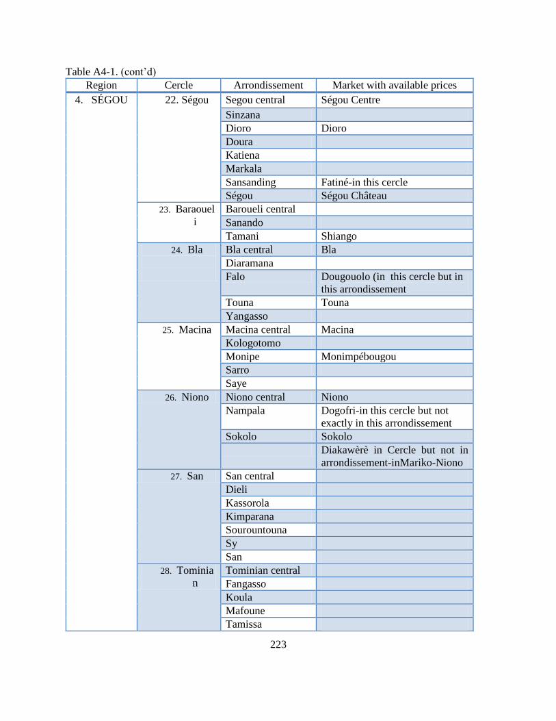
223
Table A4-1. (cont’d)
Region Cercle Arrondissement Market with available prices
4. SÉGOU 22. Ségou Segou central Ségou Centre
Sinzana
Dioro Dioro
Doura
Katiena
Markala
Sansanding Fatiné-in this cercle
Ségou Ségou Château
23. Baraouel
i
Baroueli central
Sanando
Tamani Shiango
24. Bla
Bla central Bla
Diaramana
Falo Dougouolo (in this cercle but in
this arrondissement
Touna Touna
Yangasso
25. Macina
Macina central Macina
Kologotomo
Monipe Monimpébougou
Sarro
Saye
26. Niono Niono central Niono
Nampala Dogofri-in this cercle but not
exactly in this arrondissement
Sokolo Sokolo
Diakawèrè in Cercle but not in
arrondissement-inMariko-Niono
27. San San central
Dieli
Kassorola
Kimparana
Sourountouna
Sy
San
28. Tominia
n
Tominian central
Fangasso
Koula
Mafoune
Tamissa
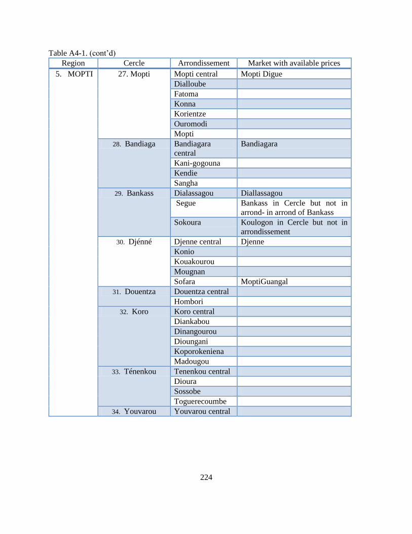
224
Table A4-1. (cont’d)
Region Cercle Arrondissement Market with available prices
5. MOPTI 27. Mopti Mopti central Mopti Digue
Dialloube
Fatoma
Konna
Korientze
Ouromodi
Mopti
28. Bandiaga Bandiagara
central
Bandiagara
Kani-gogouna
Kendie
Sangha
29. Bankass Dialassagou Diallassagou
Segue Bankass in Cercle but not in
arrond- in arrond of Bankass
Sokoura Koulogon in Cercle but not in
arrondissement
30. Djénné Djenne central Djenne
Konio
Kouakourou
Mougnan
Sofara MoptiGuangal
31. Douentza Douentza central
Hombori
32. Koro Koro central
Diankabou
Dinangourou
Dioungani
Koporokeniena
Madougou
33. Ténenkou Tenenkou central
Dioura
Sossobe
Toguerecoumbe
34. Youvarou Youvarou central
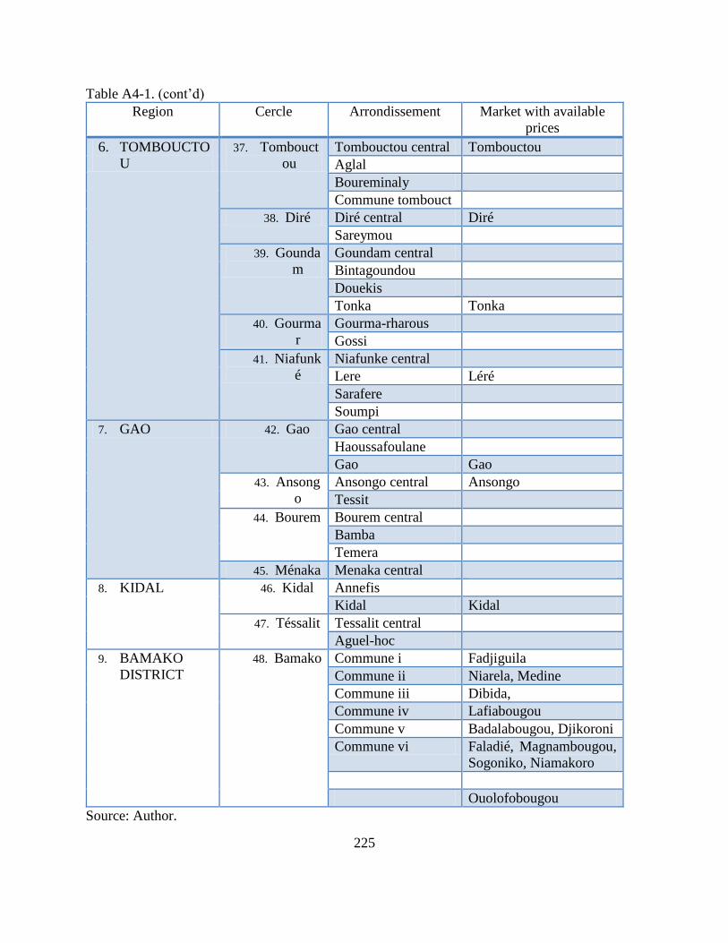
225
Table A4-1. (cont’d)
Region Cercle Arrondissement Market with available
prices
6. TOMBOUCTO
U
37. Tombouct
ou
Tombouctou central Tombouctou
Aglal
Boureminaly
Commune tombouct
38. Diré Diré central Diré
Sareymou
39. Gounda
m
Goundam central
Bintagoundou
Douekis
Tonka Tonka
40. Gourma
r
Gourma-rharous
Gossi
41. Niafunk
é
Niafunke central
Lere Léré
Sarafere
Soumpi
7. GAO 42. Gao Gao central
Haoussafoulane
Gao Gao
43. Ansong
o
Ansongo central Ansongo
Tessit
44. Bourem Bourem central
Bamba
Temera
45. Ménaka Menaka central
8. KIDAL 46. Kidal Annefis
Kidal Kidal
47. Téssalit Tessalit central
Aguel-hoc
9. BAMAKO
DISTRICT
48. Bamako Commune i Fadjiguila
Commune ii Niarela, Medine
Commune iii Dibida,
Commune iv Lafiabougou
Commune v Badalabougou, Djikoroni
Commune vi Faladié, Magnambougou,
Sogoniko, Niamakoro
Ouolofobougou
Source: Author.
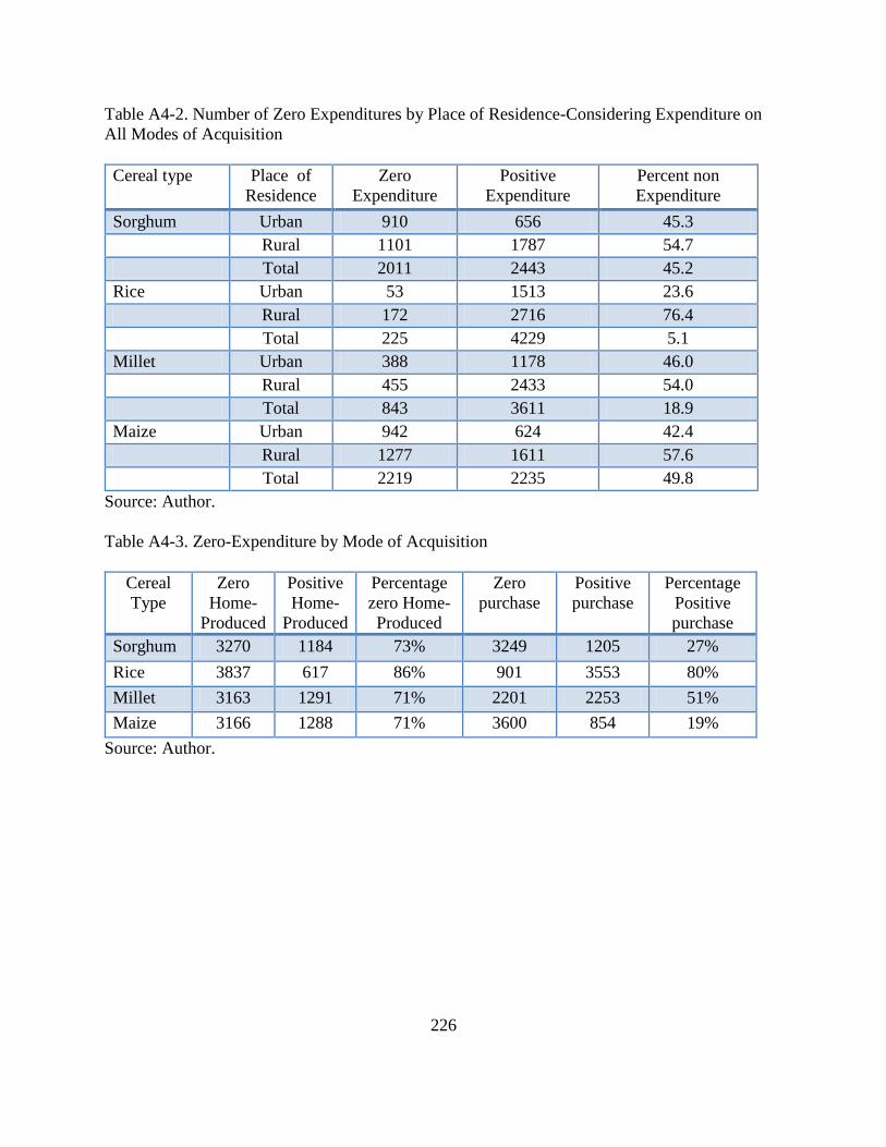
226
Table A4-2. Number of Zero Expenditures by Place of Residence-Considering Expenditure on
All Modes of Acquisition
Cereal type Place of
Residence
Zero
Expenditure
Positive
Expenditure
Percent non
Expenditure
Sorghum Urban 910 656 45.3
Rural 1101 1787 54.7
Total 2011 2443 45.2
Rice Urban 53 1513 23.6
Rural 172 2716 76.4
Total 225 4229 5.1
Millet Urban 388 1178 46.0
Rural 455 2433 54.0
Total 843 3611 18.9
Maize Urban 942 624 42.4
Rural 1277 1611 57.6
Total 2219 2235 49.8
Source: Author.
Table A4-3. Zero-Expenditure by Mode of Acquisition
Cereal
Type
Zero
Home-
Produced
Positive
Home-
Produced
Percentage
zero Home-
Produced
Zero
purchase
Positive
purchase
Percentage
Positive
purchase
Sorghum 3270 1184 73% 3249 1205 27%
Rice 3837 617 86% 901 3553 80%
Millet 3163 1291 71% 2201 2253 51%
Maize 3166 1288 71% 3600 854 19%
Source: Author.
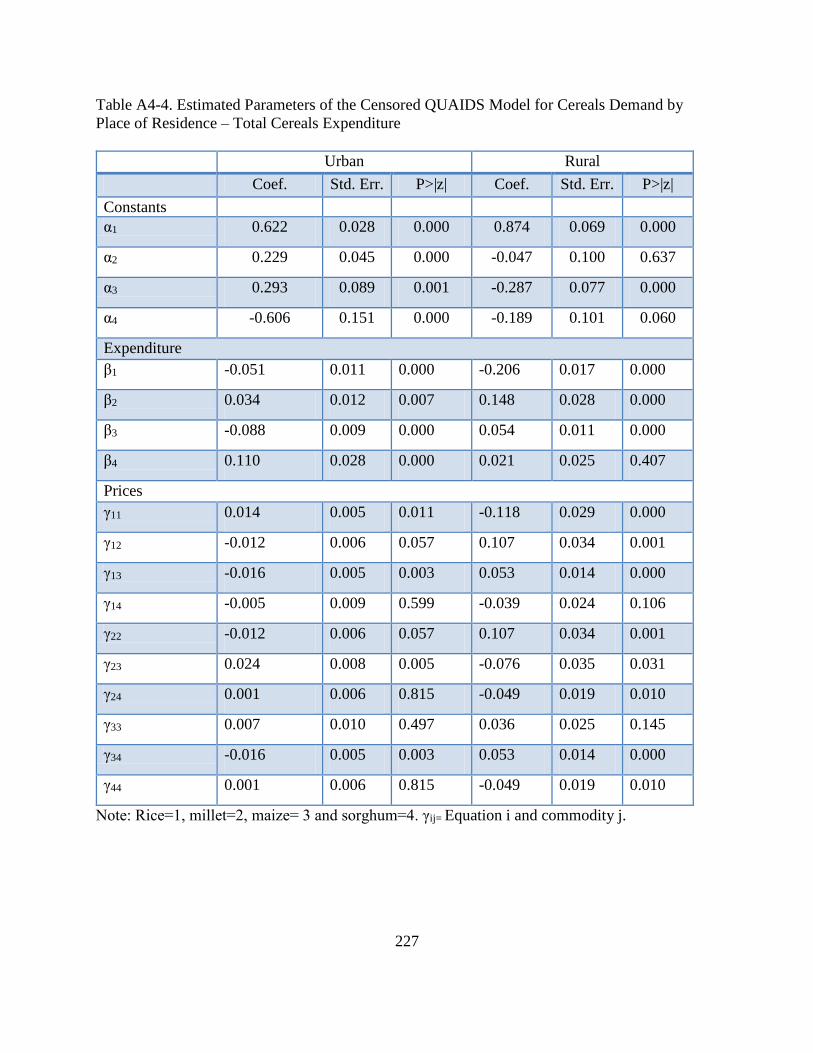
227
Table A4-4. Estimated Parameters of the Censored QUAIDS Model for Cereals Demand by
Place of Residence – Total Cereals Expenditure
Urban Rural
Coef. Std. Err. P>|z| Coef. Std. Err. P>|z|
Constants
α1 0.622 0.028 0.000 0.874 0.069 0.000
α2 0.229 0.045 0.000 -0.047 0.100 0.637
α3 0.293 0.089 0.001 -0.287 0.077 0.000
α4 -0.606 0.151 0.000 -0.189 0.101 0.060
Expenditure
β1 -0.051 0.011 0.000 -0.206 0.017 0.000
β2 0.034 0.012 0.007 0.148 0.028 0.000
β3 -0.088 0.009 0.000 0.054 0.011 0.000
β4 0.110 0.028 0.000 0.021 0.025 0.407
Prices
γ11 0.014 0.005 0.011 -0.118 0.029 0.000
γ12 -0.012 0.006 0.057 0.107 0.034 0.001
γ13 -0.016 0.005 0.003 0.053 0.014 0.000
γ14 -0.005 0.009 0.599 -0.039 0.024 0.106
γ22 -0.012 0.006 0.057 0.107 0.034 0.001
γ23 0.024 0.008 0.005 -0.076 0.035 0.031
γ24 0.001 0.006 0.815 -0.049 0.019 0.010
γ33 0.007 0.010 0.497 0.036 0.025 0.145
γ34 -0.016 0.005 0.003 0.053 0.014 0.000
γ44 0.001 0.006 0.815 -0.049 0.019 0.010
Note: Rice=1, millet=2, maize= 3 and sorghum=4. γij= Equation i and commodity j.
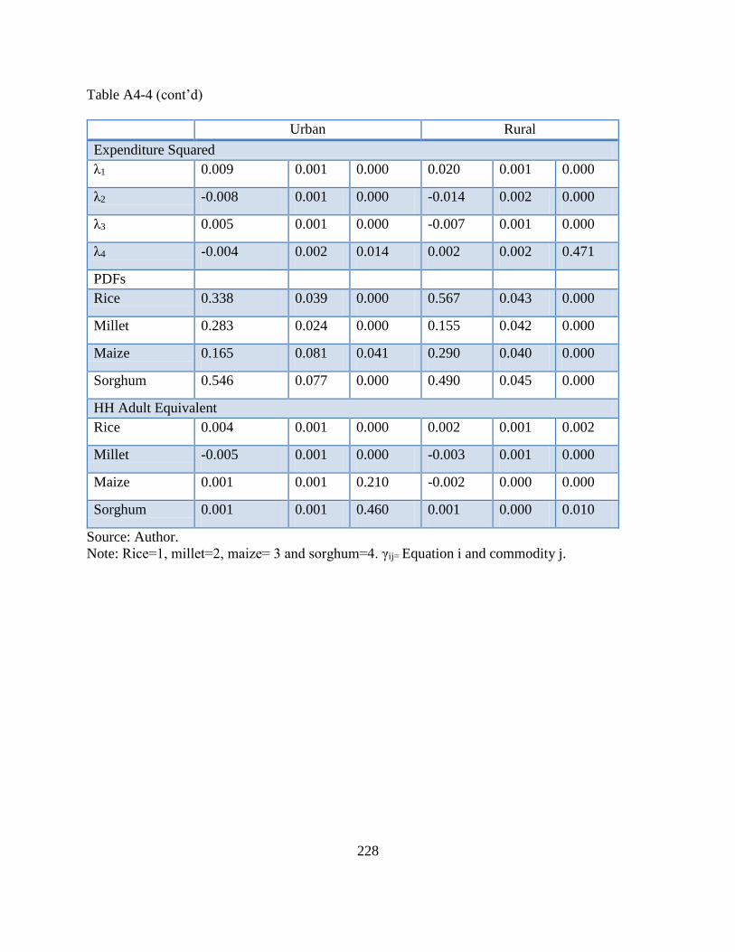
228
Table A4-4 (cont’d)
Urban Rural
Expenditure Squared
λ1 0.009 0.001 0.000 0.020 0.001 0.000
λ2 -0.008 0.001 0.000 -0.014 0.002 0.000
λ3 0.005 0.001 0.000 -0.007 0.001 0.000
λ4 -0.004 0.002 0.014 0.002 0.002 0.471
PDFs
Rice 0.338 0.039 0.000 0.567 0.043 0.000
Millet 0.283 0.024 0.000 0.155 0.042 0.000
Maize 0.165 0.081 0.041 0.290 0.040 0.000
Sorghum 0.546 0.077 0.000 0.490 0.045 0.000
HH Adult Equivalent
Rice 0.004 0.001 0.000 0.002 0.001 0.002
Millet -0.005 0.001 0.000 -0.003 0.001 0.000
Maize 0.001 0.001 0.210 -0.002 0.000 0.000
Sorghum 0.001 0.001 0.460 0.001 0.000 0.010
Source: Author.
Note: Rice=1, millet=2, maize= 3 and sorghum=4. γij= Equation i and commodity j.
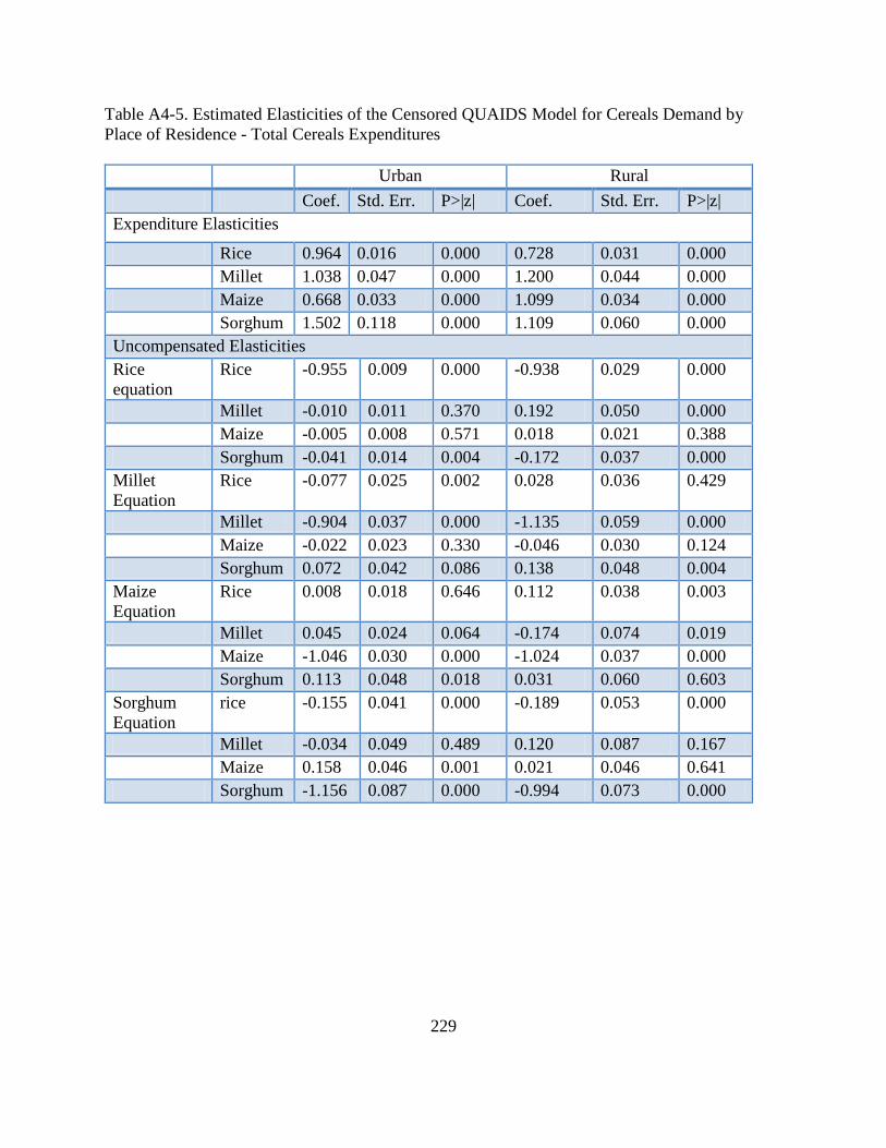
229
Table A4-5. Estimated Elasticities of the Censored QUAIDS Model for Cereals Demand by
Place of Residence - Total Cereals Expenditures
Urban Rural
Coef. Std. Err. P>|z| Coef. Std. Err. P>|z|
Expenditure Elasticities
Rice 0.964 0.016 0.000 0.728 0.031 0.000
Millet 1.038 0.047 0.000 1.200 0.044 0.000
Maize 0.668 0.033 0.000 1.099 0.034 0.000
Sorghum 1.502 0.118 0.000 1.109 0.060 0.000
Uncompensated Elasticities
Rice
equation
Rice -0.955 0.009 0.000 -0.938 0.029 0.000
Millet -0.010 0.011 0.370 0.192 0.050 0.000
Maize -0.005 0.008 0.571 0.018 0.021 0.388
Sorghum -0.041 0.014 0.004 -0.172 0.037 0.000
Millet
Equation
Rice -0.077 0.025 0.002 0.028 0.036 0.429
Millet -0.904 0.037 0.000 -1.135 0.059 0.000
Maize -0.022 0.023 0.330 -0.046 0.030 0.124
Sorghum 0.072 0.042 0.086 0.138 0.048 0.004
Maize
Equation
Rice 0.008 0.018 0.646 0.112 0.038 0.003
Millet 0.045 0.024 0.064 -0.174 0.074 0.019
Maize -1.046 0.030 0.000 -1.024 0.037 0.000
Sorghum 0.113 0.048 0.018 0.031 0.060 0.603
Sorghum
Equation
rice -0.155 0.041 0.000 -0.189 0.053 0.000
Millet -0.034 0.049 0.489 0.120 0.087 0.167
Maize 0.158 0.046 0.001 0.021 0.046 0.641
Sorghum -1.156 0.087 0.000 -0.994 0.073 0.000
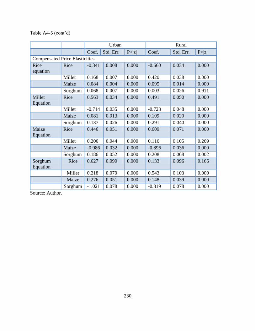
230
Table A4-5 (cont’d)
Urban Rural
Coef. Std. Err. P>|z| Coef. Std. Err. P>|z|
Compensated Price Elasticities
Rice
equation
Rice -0.341 0.008 0.000 -0.660 0.034 0.000
Millet 0.168 0.007 0.000 0.420 0.038 0.000
Maize 0.084 0.004 0.000 0.095 0.014 0.000
Sorghum 0.068 0.007 0.000 0.003 0.026 0.911
Millet
Equation
Rice 0.563 0.034 0.000 0.491 0.050 0.000
Millet -0.714 0.035 0.000 -0.723 0.048 0.000
Maize 0.081 0.013 0.000 0.109 0.020 0.000
Sorghum 0.137 0.026 0.000 0.291 0.040 0.000
Maize
Equation
Rice 0.446 0.051 0.000 0.609 0.071 0.000
Millet 0.206 0.044 0.000 0.116 0.105 0.269
Maize -0.986 0.032 0.000 -0.896 0.036 0.000
Sorghum 0.186 0.052 0.000 0.208 0.068 0.002
Sorghum
Equation
Rice 0.627 0.090 0.000 0.133 0.096 0.166
Millet 0.218 0.079 0.006 0.543 0.103 0.000
Maize 0.276 0.051 0.000 0.148 0.039 0.000
Sorghum -1.021 0.078 0.000 -0.819 0.078 0.000
Source: Author.
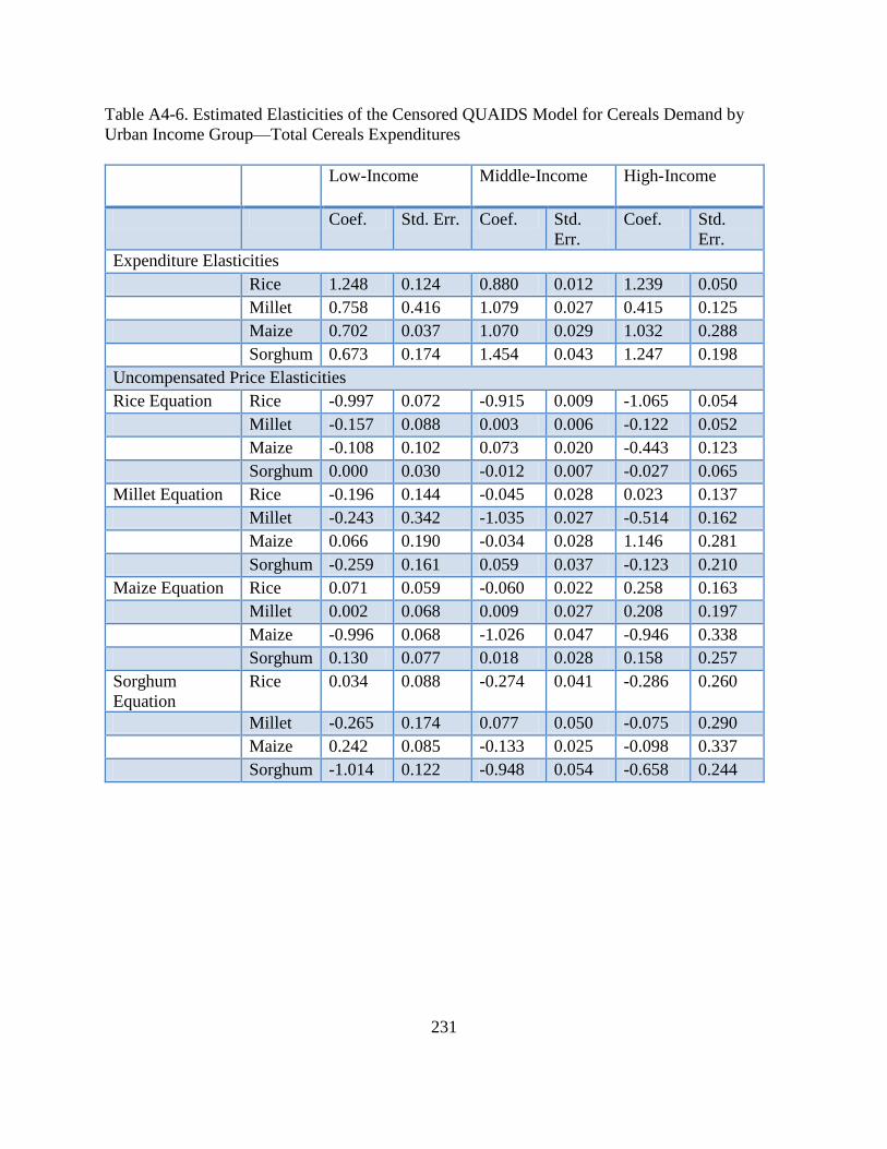
231
Table A4-6. Estimated Elasticities of the Censored QUAIDS Model for Cereals Demand by
Urban Income Group—Total Cereals Expenditures
Low-Income
Middle-Income High-Income
Coef. Std. Err. Coef. Std.
Err.
Coef. Std.
Err.
Expenditure Elasticities
Rice 1.248 0.124 0.880 0.012 1.239 0.050
Millet 0.758 0.416 1.079 0.027 0.415 0.125
Maize 0.702 0.037 1.070 0.029 1.032 0.288
Sorghum 0.673 0.174 1.454 0.043 1.247 0.198
Uncompensated Price Elasticities
Rice Equation Rice -0.997 0.072 -0.915 0.009 -1.065 0.054
Millet -0.157 0.088 0.003 0.006 -0.122 0.052
Maize -0.108 0.102 0.073 0.020 -0.443 0.123
Sorghum 0.000 0.030 -0.012 0.007 -0.027 0.065
Millet Equation Rice -0.196 0.144 -0.045 0.028 0.023 0.137
Millet -0.243 0.342 -1.035 0.027 -0.514 0.162
Maize 0.066 0.190 -0.034 0.028 1.146 0.281
Sorghum -0.259 0.161 0.059 0.037 -0.123 0.210
Maize Equation Rice 0.071 0.059 -0.060 0.022 0.258 0.163
Millet 0.002 0.068 0.009 0.027 0.208 0.197
Maize -0.996 0.068 -1.026 0.047 -0.946 0.338
Sorghum 0.130 0.077 0.018 0.028 0.158 0.257
Sorghum
Equation
Rice 0.034 0.088 -0.274 0.041 -0.286 0.260
Millet -0.265 0.174 0.077 0.050 -0.075 0.290
Maize 0.242 0.085 -0.133 0.025 -0.098 0.337
Sorghum -1.014 0.122 -0.948 0.054 -0.658 0.244
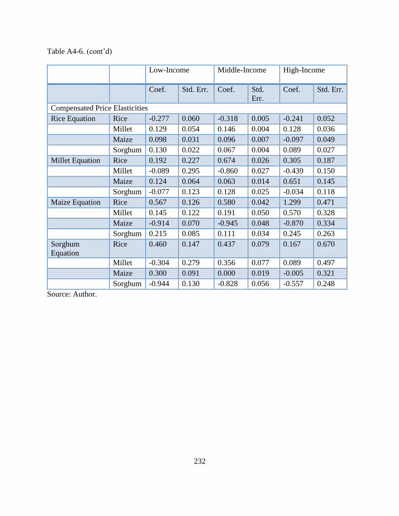
232
Table A4-6. (cont’d)
Low-Income
Middle-Income High-Income
Coef. Std. Err. Coef. Std.
Err.
Coef. Std. Err.
Compensated Price Elasticities
Rice Equation Rice -0.277 0.060 -0.318 0.005 -0.241 0.052
Millet 0.129 0.054 0.146 0.004 0.128 0.036
Maize 0.098 0.031 0.096 0.007 -0.097 0.049
Sorghum 0.130 0.022 0.067 0.004 0.089 0.027
Millet Equation Rice 0.192 0.227 0.674 0.026 0.305 0.187
Millet -0.089 0.295 -0.860 0.027 -0.439 0.150
Maize 0.124 0.064 0.063 0.014 0.651 0.145
Sorghum -0.077 0.123 0.128 0.025 -0.034 0.118
Maize Equation Rice 0.567 0.126 0.580 0.042 1.299 0.471
Millet 0.145 0.122 0.191 0.050 0.570 0.328
Maize -0.914 0.070 -0.945 0.048 -0.870 0.334
Sorghum 0.215 0.085 0.111 0.034 0.245 0.263
Sorghum
Equation
Rice 0.460 0.147 0.437 0.079 0.167 0.670
Millet -0.304 0.279 0.356 0.077 0.089 0.497
Maize 0.300 0.091 0.000 0.019 -0.005 0.321
Sorghum -0.944 0.130 -0.828 0.056 -0.557 0.248
Source: Author.
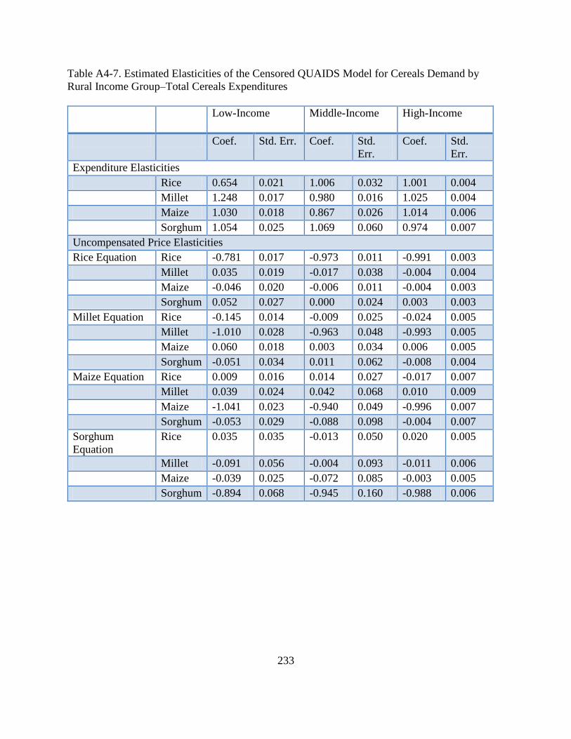
233
Table A4-7. Estimated Elasticities of the Censored QUAIDS Model for Cereals Demand by
Rural Income Group–Total Cereals Expenditures
Low-Income
Middle-Income High-Income
Coef. Std. Err. Coef. Std.
Err.
Coef. Std.
Err.
Expenditure Elasticities
Rice 0.654 0.021 1.006 0.032 1.001 0.004
Millet 1.248 0.017 0.980 0.016 1.025 0.004
Maize 1.030 0.018 0.867 0.026 1.014 0.006
Sorghum 1.054 0.025 1.069 0.060 0.974 0.007
Uncompensated Price Elasticities
Rice Equation Rice -0.781 0.017 -0.973 0.011 -0.991 0.003
Millet 0.035 0.019 -0.017 0.038 -0.004 0.004
Maize -0.046 0.020 -0.006 0.011 -0.004 0.003
Sorghum 0.052 0.027 0.000 0.024 0.003 0.003
Millet Equation Rice -0.145 0.014 -0.009 0.025 -0.024 0.005
Millet -1.010 0.028 -0.963 0.048 -0.993 0.005
Maize 0.060 0.018 0.003 0.034 0.006 0.005
Sorghum -0.051 0.034 0.011 0.062 -0.008 0.004
Maize Equation Rice 0.009 0.016 0.014 0.027 -0.017 0.007
Millet 0.039 0.024 0.042 0.068 0.010 0.009
Maize -1.041 0.023 -0.940 0.049 -0.996 0.007
Sorghum -0.053 0.029 -0.088 0.098 -0.004 0.007
Sorghum
Equation
Rice 0.035 0.035 -0.013 0.050 0.020 0.005
Millet -0.091 0.056 -0.004 0.093 -0.011 0.006
Maize -0.039 0.025 -0.072 0.085 -0.003 0.005
Sorghum -0.894 0.068 -0.945 0.160 -0.988 0.006
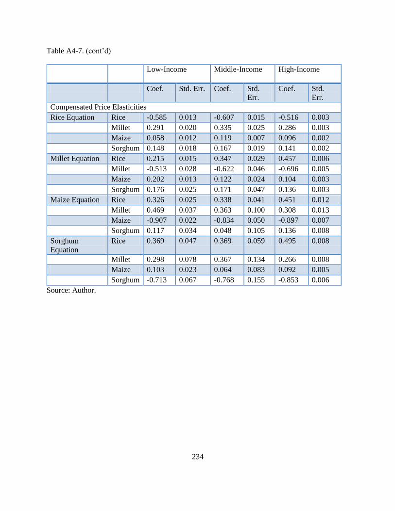
234
Table A4-7. (cont’d)
Low-Income
Middle-Income High-Income
Coef. Std. Err. Coef. Std.
Err.
Coef. Std.
Err.
Compensated Price Elasticities
Rice Equation Rice -0.585 0.013 -0.607 0.015 -0.516 0.003
Millet 0.291 0.020 0.335 0.025 0.286 0.003
Maize 0.058 0.012 0.119 0.007 0.096 0.002
Sorghum 0.148 0.018 0.167 0.019 0.141 0.002
Millet Equation Rice 0.215 0.015 0.347 0.029 0.457 0.006
Millet -0.513 0.028 -0.622 0.046 -0.696 0.005
Maize 0.202 0.013 0.122 0.024 0.104 0.003
Sorghum 0.176 0.025 0.171 0.047 0.136 0.003
Maize Equation Rice 0.326 0.025 0.338 0.041 0.451 0.012
Millet 0.469 0.037 0.363 0.100 0.308 0.013
Maize -0.907 0.022 -0.834 0.050 -0.897 0.007
Sorghum 0.117 0.034 0.048 0.105 0.136 0.008
Sorghum
Equation
Rice 0.369 0.047 0.369 0.059 0.495 0.008
Millet 0.298 0.078 0.367 0.134 0.266 0.008
Maize 0.103 0.023 0.064 0.083 0.092 0.005
Sorghum -0.713 0.067 -0.768 0.155 -0.853 0.006
Source: Author.
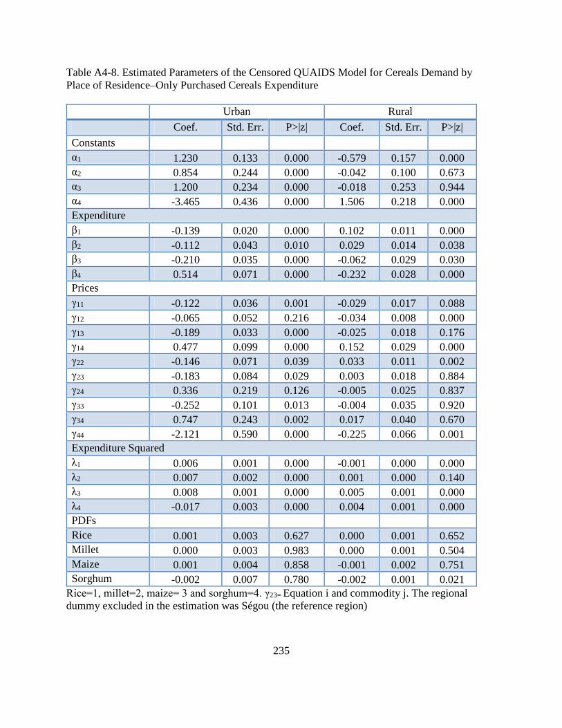
235
Table A4-8. Estimated Parameters of the Censored QUAIDS Model for Cereals Demand by
Place of Residence–Only Purchased Cereals Expenditure
Urban Rural
Coef. Std. Err. P>|z| Coef. Std. Err. P>|z|
Constants
α1 1.230 0.133 0.000 -0.579 0.157 0.000
α2 0.854 0.244 0.000 -0.042 0.100 0.673
α3 1.200 0.234 0.000 -0.018 0.253 0.944
α4 -3.465 0.436 0.000 1.506 0.218 0.000
Expenditure
β1 -0.139 0.020 0.000 0.102 0.011 0.000
β2 -0.112 0.043 0.010 0.029 0.014 0.038
β3 -0.210 0.035 0.000 -0.062 0.029 0.030
β4 0.514 0.071 0.000 -0.232 0.028 0.000
Prices
γ11 -0.122 0.036 0.001 -0.029 0.017 0.088
γ12 -0.065 0.052 0.216 -0.034 0.008 0.000
γ13 -0.189 0.033 0.000 -0.025 0.018 0.176
γ14 0.477 0.099 0.000 0.152 0.029 0.000
γ22 -0.146 0.071 0.039 0.033 0.011 0.002
γ23 -0.183 0.084 0.029 0.003 0.018 0.884
γ24 0.336 0.219 0.126 -0.005 0.025 0.837
γ33 -0.252 0.101 0.013 -0.004 0.035 0.920
γ34 0.747 0.243 0.002 0.017 0.040 0.670
γ44 -2.121 0.590 0.000 -0.225 0.066 0.001
Expenditure Squared
λ1 0.006 0.001 0.000 -0.001 0.000 0.000
λ2 0.007 0.002 0.000 0.001 0.000 0.140
λ3 0.008 0.001 0.000 0.005 0.001 0.000
λ4 -0.017 0.003 0.000 0.004 0.001 0.000
PDFs
Rice 0.001 0.003 0.627 0.000 0.001 0.652
Millet 0.000 0.003 0.983 0.000 0.001 0.504
Maize 0.001 0.004 0.858 -0.001 0.002 0.751
Sorghum -0.002 0.007 0.780 -0.002 0.001 0.021
Rice=1, millet=2, maize= 3 and sorghum=4. γ23= Equation i and commodity j. The regional
dummy excluded in the estimation was Ségou (the reference region)
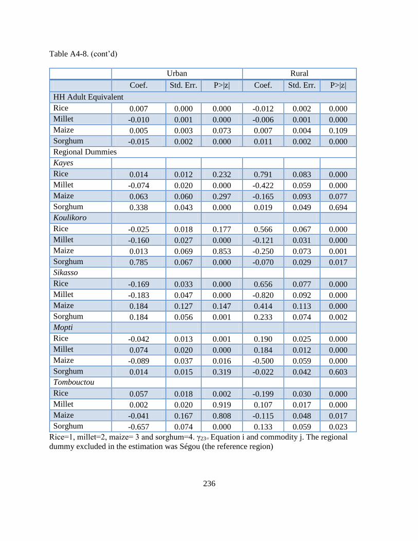
236
Table A4-8. (cont’d)
Urban Rural
Coef. Std. Err. P>|z| Coef. Std. Err. P>|z|
HH Adult Equivalent
Rice 0.007 0.000 0.000 -0.012 0.002 0.000
Millet -0.010 0.001 0.000 -0.006 0.001 0.000
Maize 0.005 0.003 0.073 0.007 0.004 0.109
Sorghum -0.015 0.002 0.000 0.011 0.002 0.000
Regional Dummies
Kayes
Rice 0.014 0.012 0.232 0.791 0.083 0.000
Millet -0.074 0.020 0.000 -0.422 0.059 0.000
Maize 0.063 0.060 0.297 -0.165 0.093 0.077
Sorghum 0.338 0.043 0.000 0.019 0.049 0.694
Koulikoro
Rice -0.025 0.018 0.177 0.566 0.067 0.000
Millet -0.160 0.027 0.000 -0.121 0.031 0.000
Maize 0.013 0.069 0.853 -0.250 0.073 0.001
Sorghum 0.785 0.067 0.000 -0.070 0.029 0.017
Sikasso
Rice -0.169 0.033 0.000 0.656 0.077 0.000
Millet -0.183 0.047 0.000 -0.820 0.092 0.000
Maize 0.184 0.127 0.147 0.414 0.113 0.000
Sorghum 0.184 0.056 0.001 0.233 0.074 0.002
Mopti
Rice -0.042 0.013 0.001 0.190 0.025 0.000
Millet 0.074 0.020 0.000 0.184 0.012 0.000
Maize -0.089 0.037 0.016 -0.500 0.059 0.000
Sorghum 0.014 0.015 0.319 -0.022 0.042 0.603
Tombouctou
Rice 0.057 0.018 0.002 -0.199 0.030 0.000
Millet 0.002 0.020 0.919 0.107 0.017 0.000
Maize -0.041 0.167 0.808 -0.115 0.048 0.017
Sorghum -0.657 0.074 0.000 0.133 0.059 0.023
Rice=1, millet=2, maize= 3 and sorghum=4. γ23= Equation i and commodity j. The regional
dummy excluded in the estimation was Ségou (the reference region)
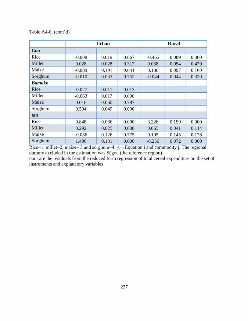
237
Table A4-8. (cont’d)
Urban Rural
Gao
Rice -0.008 0.019 0.667 -0.465 0.089 0.000
Millet 0.028 0.028 0.317 0.038 0.054 0.479
Maize -0.089 0.191 0.641 0.136 0.097 0.160
Sorghum -0.010 0.033 0.752 -0.044 0.044 0.320
Bamako
Rice -0.027 0.011 0.013
Millet -0.063 0.017 0.000
Maize 0.016 0.060 0.787
Sorghum 0.504 0.049 0.000
tau
Rice 0.848 0.086 0.000 3.226 0.199 0.000
Millet 0.292 0.025 0.000 0.065 0.041 0.114
Maize -0.036 0.126 0.775 0.195 0.145 0.178
Sorghum 1.496 0.131 0.000 -0.256 0.072 0.000
Rice=1, millet=2, maize= 3 and sorghum=4. γ23= Equation i and commodity j. The regional
dummy excluded in the estimation was Ségou (the reference region)
tau - are the residuals from the reduced form regression of total cereal expenditure on the set of
instruments and explanatory variables
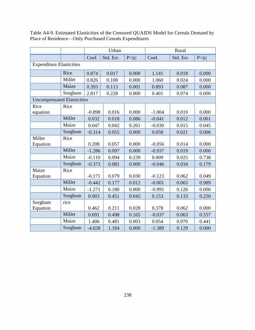
238
Table A4-9. Estimated Elasticities of the Censored QUAIDS Model for Cereals Demand by
Place of Residence—Only Purchased Cereals Expenditures
Urban Rural
Coef. Std. Err. P>|z| Coef. Std. Err. P>|z|
Expenditure Elasticities
Rice 0.874 0.017 0.000 1.141 0.018 0.000
Millet 0.826 0.108 0.000 1.060 0.024 0.000
Maize 0.393 0.113 0.001 0.893 0.087 0.000
Sorghum 2.817 0.228 0.000 0.401 0.074 0.000
Uncompensated Elasticities
Rice
equation
Rice
-0.898 0.016 0.000 -1.004 0.010 0.000
Millet 0.032 0.018 0.086 -0.041 0.012 0.001
Maize 0.047 0.042 0.261 -0.030 0.015 0.045
Sorghum -0.314 0.055 0.000 0.058 0.021 0.006
Millet
Equation
Rice
0.208 0.057 0.000 -0.056 0.014 0.000
Millet -1.286 0.097 0.000 -0.937 0.019 0.000
Maize -0.110 0.094 0.239 0.009 0.025 0.738
Sorghum -0.373 0.081 0.000 -0.046 0.034 0.179
Maize
Equation
Rice
-0.171 0.079 0.030 -0.123 0.062 0.049
Millet -0.442 0.177 0.012 -0.001 0.065 0.989
Maize -1.271 0.180 0.000 -0.995 0.126 0.000
Sorghum 0.903 0.451 0.045 0.153 0.133 0.250
Sorghum
Equation
rice
0.462 0.211 0.028 0.378 0.062 0.000
Millet 0.691 0.498 0.165 -0.037 0.063 0.557
Maize 1.406 0.481 0.003 0.054 0.070 0.441
Sorghum -4.658 1.184 0.000 -1.389 0.129 0.000
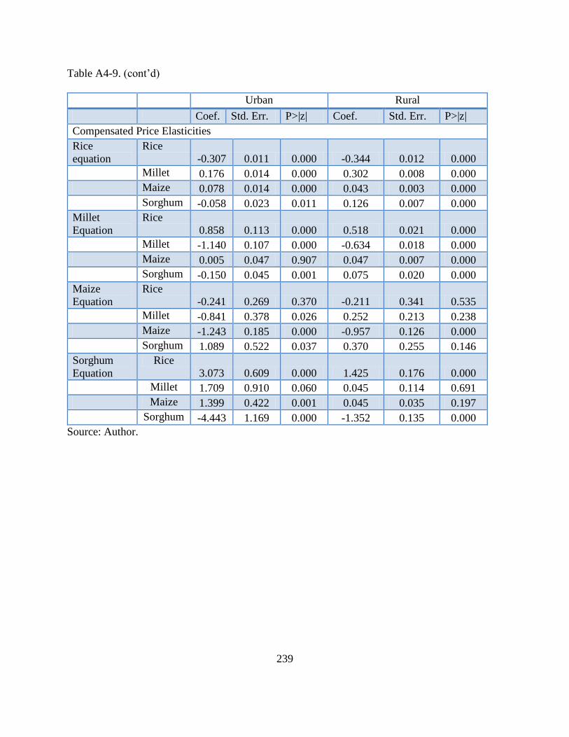
239
Table A4-9. (cont’d)
Urban Rural
Coef. Std. Err. P>|z| Coef. Std. Err. P>|z|
Compensated Price Elasticities
Rice
equation
Rice
-0.307 0.011 0.000 -0.344 0.012 0.000
Millet 0.176 0.014 0.000 0.302 0.008 0.000
Maize 0.078 0.014 0.000 0.043 0.003 0.000
Sorghum -0.058 0.023 0.011 0.126 0.007 0.000
Millet
Equation
Rice
0.858 0.113 0.000 0.518 0.021 0.000
Millet -1.140 0.107 0.000 -0.634 0.018 0.000
Maize 0.005 0.047 0.907 0.047 0.007 0.000
Sorghum -0.150 0.045 0.001 0.075 0.020 0.000
Maize
Equation
Rice
-0.241 0.269 0.370 -0.211 0.341 0.535
Millet -0.841 0.378 0.026 0.252 0.213 0.238
Maize -1.243 0.185 0.000 -0.957 0.126 0.000
Sorghum 1.089 0.522 0.037 0.370 0.255 0.146
Sorghum
Equation
Rice
3.073 0.609 0.000 1.425 0.176 0.000
Millet 1.709 0.910 0.060 0.045 0.114 0.691
Maize 1.399 0.422 0.001 0.045 0.035 0.197
Sorghum -4.443 1.169 0.000 -1.352 0.135 0.000
Source: Author.
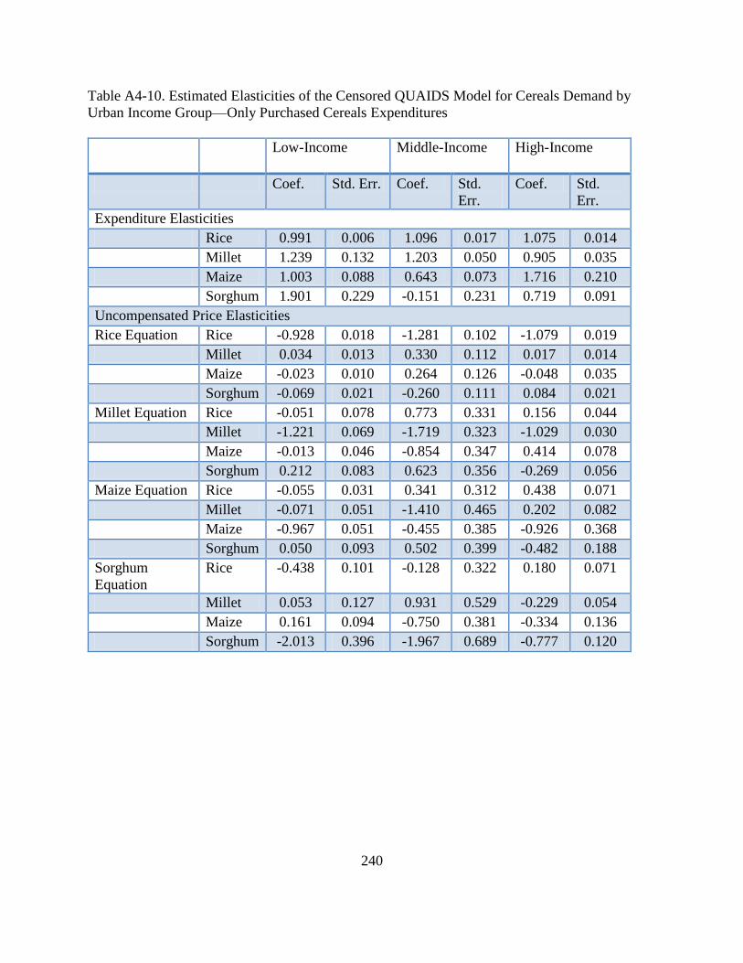
240
Table A4-10. Estimated Elasticities of the Censored QUAIDS Model for Cereals Demand by
Urban Income Group—Only Purchased Cereals Expenditures
Low-Income
Middle-Income High-Income
Coef. Std. Err. Coef. Std.
Err.
Coef. Std.
Err.
Expenditure Elasticities
Rice 0.991 0.006 1.096 0.017 1.075 0.014
Millet 1.239 0.132 1.203 0.050 0.905 0.035
Maize 1.003 0.088 0.643 0.073 1.716 0.210
Sorghum 1.901 0.229 -0.151 0.231 0.719 0.091
Uncompensated Price Elasticities
Rice Equation Rice -0.928 0.018 -1.281 0.102 -1.079 0.019
Millet 0.034 0.013 0.330 0.112 0.017 0.014
Maize -0.023 0.010 0.264 0.126 -0.048 0.035
Sorghum -0.069 0.021 -0.260 0.111 0.084 0.021
Millet Equation Rice -0.051 0.078 0.773 0.331 0.156 0.044
Millet -1.221 0.069 -1.719 0.323 -1.029 0.030
Maize -0.013 0.046 -0.854 0.347 0.414 0.078
Sorghum 0.212 0.083 0.623 0.356 -0.269 0.056
Maize Equation Rice -0.055 0.031 0.341 0.312 0.438 0.071
Millet -0.071 0.051 -1.410 0.465 0.202 0.082
Maize -0.967 0.051 -0.455 0.385 -0.926 0.368
Sorghum 0.050 0.093 0.502 0.399 -0.482 0.188
Sorghum
Equation
Rice -0.438 0.101 -0.128 0.322 0.180 0.071
Millet 0.053 0.127 0.931 0.529 -0.229 0.054
Maize 0.161 0.094 -0.750 0.381 -0.334 0.136
Sorghum -2.013 0.396 -1.967 0.689 -0.777 0.120
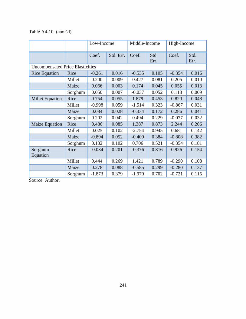
241
Table A4-10. (cont’d)
Low-Income
Middle-Income High-Income
Coef. Std. Err. Coef. Std.
Err.
Coef. Std.
Err.
Uncompensated Price Elasticities
Rice Equation Rice -0.261 0.016 -0.535 0.105 -0.354 0.016
Millet 0.200 0.009 0.427 0.081 0.205 0.010
Maize 0.066 0.003 0.174 0.045 0.055 0.013
Sorghum 0.050 0.007 -0.037 0.052 0.118 0.009
Millet Equation Rice 0.754 0.055 1.879 0.453 0.820 0.048
Millet -0.998 0.059 -1.514 0.323 -0.867 0.031
Maize 0.084 0.028 -0.334 0.172 0.286 0.041
Sorghum 0.202 0.042 0.494 0.229 -0.077 0.032
Maize Equation Rice 0.486 0.085 1.387 0.873 2.244 0.206
Millet 0.025 0.102 -2.754 0.945 0.681 0.142
Maize -0.894 0.052 -0.409 0.384 -0.808 0.382
Sorghum 0.132 0.102 0.706 0.521 -0.354 0.181
Sorghum
Equation
Rice -0.034 0.201 -0.376 0.816 0.926 0.154
Millet 0.444 0.269 1.421 0.789 -0.290 0.108
Maize 0.278 0.088 -0.585 0.299 -0.280 0.137
Sorghum -1.873 0.379 -1.979 0.702 -0.721 0.115
Source: Author.
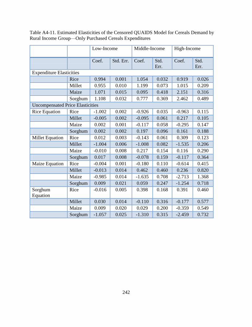
242
Table A4-11. Estimated Elasticities of the Censored QUAIDS Model for Cereals Demand by
Rural Income Group—Only Purchased Cereals Expenditures
Low-Income
Middle-Income High-Income
Coef. Std. Err. Coef. Std.
Err.
Coef. Std.
Err.
Expenditure Elasticities
Rice 0.994 0.001 1.054 0.032 0.919 0.026
Millet 0.955 0.010 1.199 0.073 1.015 0.209
Maize 1.071 0.015 0.095 0.418 2.151 0.316
Sorghum 1.108 0.032 0.777 0.369 2.462 0.489
Uncompensated Price Elasticities
Rice Equation Rice -1.002 0.002 -0.926 0.035 -0.963 0.115
Millet -0.005 0.002 -0.095 0.061 0.217 0.105
Maize 0.002 0.001 -0.117 0.058 -0.295 0.147
Sorghum 0.002 0.002 0.197 0.096 0.161 0.188
Millet Equation Rice 0.012 0.003 -0.143 0.061 0.309 0.123
Millet -1.004 0.006 -1.008 0.082 -1.535 0.206
Maize -0.010 0.008 0.217 0.154 0.116 0.290
Sorghum 0.017 0.008 -0.078 0.159 -0.117 0.364
Maize Equation Rice -0.004 0.001 -0.180 0.110 -0.614 0.415
Millet -0.013 0.014 0.462 0.460 0.236 0.820
Maize -0.985 0.014 -1.635 0.708 -2.713 1.368
Sorghum 0.009 0.021 0.059 0.247 -1.254 0.718
Sorghum
Equation
Rice -0.016 0.005 0.398 0.168 0.391 0.460
Millet 0.030 0.014 -0.110 0.316 -0.177 0.577
Maize 0.009 0.020 0.029 0.200 -0.359 0.549
Sorghum -1.057 0.025 -1.310 0.315 -2.459 0.732
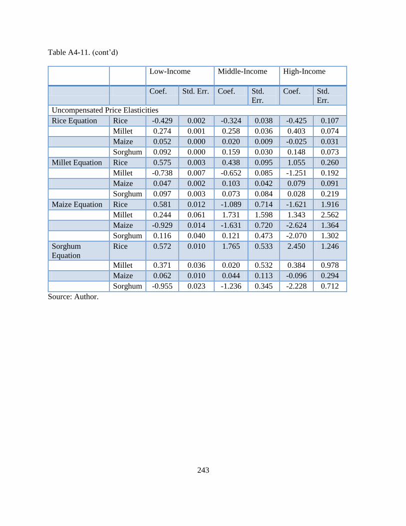
243
Table A4-11. (cont’d)
Low-Income
Middle-Income High-Income
Coef. Std. Err. Coef. Std.
Err.
Coef. Std.
Err.
Uncompensated Price Elasticities
Rice Equation Rice -0.429 0.002 -0.324 0.038 -0.425 0.107
Millet 0.274 0.001 0.258 0.036 0.403 0.074
Maize 0.052 0.000 0.020 0.009 -0.025 0.031
Sorghum 0.092 0.000 0.159 0.030 0.148 0.073
Millet Equation Rice 0.575 0.003 0.438 0.095 1.055 0.260
Millet -0.738 0.007 -0.652 0.085 -1.251 0.192
Maize 0.047 0.002 0.103 0.042 0.079 0.091
Sorghum 0.097 0.003 0.073 0.084 0.028 0.219
Maize Equation Rice 0.581 0.012 -1.089 0.714 -1.621 1.916
Millet 0.244 0.061 1.731 1.598 1.343 2.562
Maize -0.929 0.014 -1.631 0.720 -2.624 1.364
Sorghum 0.116 0.040 0.121 0.473 -2.070 1.302
Sorghum
Equation
Rice 0.572 0.010 1.765 0.533 2.450 1.246
Millet 0.371 0.036 0.020 0.532 0.384 0.978
Maize 0.062 0.010 0.044 0.113 -0.096 0.294
Sorghum -0.955 0.023 -1.236 0.345 -2.228 0.712
Source: Author.
244
CHAPTER 5. WELFARE EFFECTS OF CEREAL PRICE SHOCKS IN MALI
5.1. Problem Statement
Rice, millet, maize and sorghum are primary staple foods in Mali. Increases in cereals prices are
likely to have substantial negative impacts on the poor (see Ivanic and Martin, 2008; Joseph and
Wodon, 2008; Wodon and Zaman, 2010). Limited empirical evidence on aggregate as well as
micro-level demand parameters differentiated by important household characteristics (e.g.,
household place of residence) in Mali places a limit on policy makers’ ability to make informed
food policy decisions. If policymakers are to intervene to help those most adversely impacted by
food price changes, then policymakers need to identify those who have been most harmed and
the magnitude of that harm (Friedman and Levinsohn, 2002). Effective design of targeted actions
therefore requires knowledge of the distribution of the effects of changes in income as well as
other factors that determine food demand across different segments of the population.
5.2. Research Objectives
The goal of this chapter is to estimate the welfare effects of cereals price shocks, allowing for
second-order demand responses (substitution in demand) to cereal price changes. The study is
focused on the relative differences in the welfare effect of cereals price shocks across income
distribution and place of residence, with the goal to determine households that are most likely
affected by cereals price changes. Specifically, the analysis seeks to:
Link observed cereals price changes to changes in household welfare using the household
cereals demand parameters estimated in chapter 4 (that take into account differences in
household socio-economic and demographic characteristics, geographic location, and
place of residence) to compute a welfare measure for a cereal price change. The welfare
245
measure used in this study is a proportional compensating variation (CV) adapted from
de Janvry, et al. (2008) and that allows for substitutions in consumption.
Distinguish the welfare effects of cereals price changes by place of residence and
household per capita expenditure group.
5.3. Literature Review
A vast literature exists on the welfare implications of food price increases. The welfare effects of
changes in food prices on households can be traced through three principal channels: by affecting
the affordability of an important component of the consumption basket; by affecting the returns
from farming, insofar as the household is directly engaged in this activity; and by affecting the
demand for labor in agriculture and thus the wage income of household members who work for
agricultural producers (Aksoy and Hoekman, 2010). A fourth pathway is described in Lele and
Mellor (1972) and includes the effect of food prices on real wages and hence the impact on the
demand for labor in non-agricultural activities. Deaton (1989) observed that, as many
households in developing countries are both producers and consumers, the net impact of price
changes is determined by which effect is greater: whether the household is a net consumer/buyer
or a net producer/seller.
There has been a general consensus in the literature that first-order approximations which
focus only on the direct effects on consumption of a good resulting from a change in its price
may not be enough in evaluating the welfare consequences of food price changes. For instance
Mghenyi et al. (2011) argue that first-order approximation approaches may be restrictive for
evaluating the welfare effect of a large discrete price change because supply and demand
responses to a major price change may be substantial. When the price of a food item increases,
246
consumers can switch to cheaper/more affordable items or producers can respond to the increase
by expanding supply or reallocating inputs to capture the increase in price.
While most urban households rely on the market for almost all of their food needs, most
rural households, in contrast, are both food producers and consumers. Thus, in urban areas while
changes in food prices directly affect the affordability of the food for which the price has
increased, in the rural areas a food price increase hurts them as consumers on one hand, but on
the other hand, it has the potential of raising the incomes of food-producing households and even
that of non-food producing households through multiplier effects. Ideally, one would need to
account for second-order effects that examine not only substitution effects in consumption but
also the effects on production of food price increases, as well as the dynamic aspect (multiplier
effects— e.g., wage effects) of the food price changes (Nouve and Wodon,2008; Porto, 2005;and
Porto, 2010).
Notwithstanding, the specific approach used in examining the welfare impacts of food
price changes has been influenced by data availability and whether the interest is in measuring
short, medium or long-term effects; or static as opposed to dynamic effects. Using household
budget survey data for Mali, Joseph and Wodon (2008) provide an assessment of the short-term
impact on poverty of the increase in the price of cereals. Specifically, they examine, using
statistical analysis and non-parametric methods, both the impact on food producers (who benefit
from an increase in prices) and food consumers (who lose out when the price increases), with a
focus on poor producers and consumers. They provide estimates of the impact on poverty of
higher food prices based on a number of assumptions. First, they assume that the cost of an
increase in food prices for a household translates into an equivalent reduction of its consumption
in real terms–they do not take into account the price elasticity of demand which may lead to
247
substitution effects and thereby help offset part of the negative effect of higher prices for certain
food items. Second, they assume an increase for producers in the value of their net sales of food
translates into an increase of their consumption of equivalent size. Third, they assume that
changes in prices do not affect households when food is home-produced and consumed. To
assess impacts, they compare poverty measures obtained after the increase in prices to baseline
poverty measures. This implicitly means that they do not take into account the potential spill-
over effects of the increase in food prices for the food items included in the analysis on the prices
for items not included.
Nouve and Wodon (2008) took a step further in the work done by Joseph and Wodon
(2008) and in a dynamic general equilibrium framework estimate the broader medium-term
impact of higher rice prices in Mali on poverty. They compare a base scenario (business as
usual) to six different scenarios that combine rice price changes and policy responses (import tax
cuts on rice and measures to increase productivity of domestic rice production). They find that
considering either an 80%40 or a 110%41 increase in international rice prices from the level in
2006, a 15%42 an increase in productivity will have a larger impact than a 100% reduction in
taxes. The current study uses the same household survey data as Joseph and Wodon. However,
unlike Joseph and Wodon (2008), the study considers own-price and cross-price demand effects
in examining the welfare effects of cereals price changes. The data set covers 1566 urban
households and 2888 rural households in Mali taken from the 2006 ELIM, as described in
Chapter 4. The presence of rural households (the majority of whom are food producers and
40 This is the level of the increase actually observed in CFAF in 2008. 41 This is the level of the increase in US dollar terms. 42 An arbitrary level of productivity gains chosen for illustrative purposes.
248
consumers) warrants taking into consideration the effects of cereal price increases on cereals
demand and supply. The estimation of household supply response to food price changes,
however, requires detailed production information (e.g., production quantities/value and shares
by crop and by household, supply elasticities, etc.) which are not available in the ELIM-2006
data file. While it would be appropriate to estimate the overall welfare changes (i.e., including
producer welfare), due to data limitations on the supply side, welfare estimation in this chapter is
limited only to the consumption response (direct and substitution effects). Producer supply
response and wage effects are not taken into consideration. Consequently, the estimated impact
is considered the upper-limit of the effect of cereal price shocks on welfare.
5.4. Methodological Approach and Data
To evaluate the partial equilibrium welfare effect of cereals price changes from an initial price
level, the analysis measures a proportional compensating variation of a price change which takes
into account demand responses to a change in price. The formula for the second-order
approximation is adapted from de Janvry and Sadoulet (2008) and also used by Friedman and
Levinsohn (2002). Starting from a household’s indirect utility function, which reflects the
household’s consumption components, a second-order Taylor expansion to the indirect utility
function is used to derive a welfare measure that accounts for demand responses. The idea is that
using a set of reference prices, we can compute how well-off or worse-off households are as a
result of the price changes, moving from their initial utility level to the new utility level in
response to the changes in cereals prices. The CV is the difference between the minimum
expenditure required to achieve the original utility level (2006) at the new prices, and the initial
total expenditure–i.e., the amount of money the household would need to be given at the new set
249
of (higher) prices in order to attain the initial level of utility (2006). Approximated using a
second-order Taylor expansion of the minimum expenditure function, the CV is written as:
𝐶𝑉 ≈ ∑ 𝑤𝑖𝑑
𝑖=1
𝑑𝑙𝑛𝑝𝑖 + 0.5 [∑ ∑ 𝑤𝑖𝑑𝑒𝑖𝑗
𝑑 (𝑑𝑙𝑛𝑝𝑖)(𝑑𝑙𝑛𝑝𝑗)
𝑗=1𝑖=1
] (5 − 1)
Estimates of the compensated own (𝑒𝑖𝑖𝑑 ) and cross-price elasticities (𝑒𝑖𝑗
𝑑 ) of demand for rice,
maize, millet and sorghum by place of residence and income group are all available from chapter
4. The share of each cereal type in the household’s food budget in the initial period – 2006 (𝑤𝑖𝑑 )
is directly calculated from the survey data. 𝑑𝑙𝑛𝑝𝑖 approximates the proportionate change in the
price of commodity i. The first-order effect is captured by the first term in equation 5-1, and it
implicitly assumes zero demand elasticities (i.e., household consumption behavior remains
unaltered with price changes). The second-order effect depends on the compensated price
elasticities. From equation 5-1 it is clear that the second-order effects depend on the magnitude
of the price change as well as the relative importance of the product in purchases in the
household’s budget. Ideally, household-specific estimates are required for the computation of
household specific proportional welfare effects from price changes. To account for consumption
responses, we estimate first and second-order impacts using the budget shares and the
compensated demand elasticities.
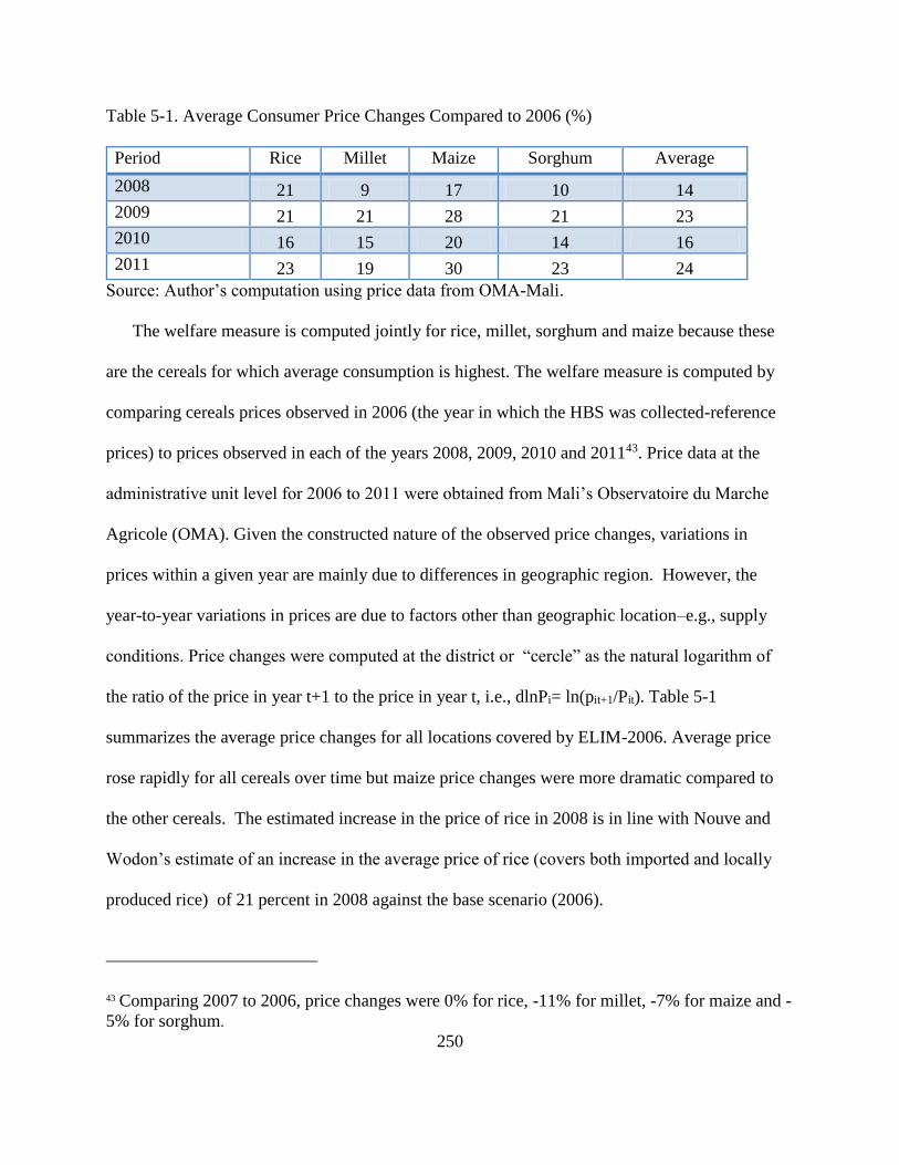
250
Table 5-1. Average Consumer Price Changes Compared to 2006 (%)
Period Rice Millet Maize Sorghum Average
2008 21 9 17 10 14
2009 21 21 28 21 23
2010 16 15 20 14 16
2011 23 19 30 23 24
Source: Author’s computation using price data from OMA-Mali.
The welfare measure is computed jointly for rice, millet, sorghum and maize because these
are the cereals for which average consumption is highest. The welfare measure is computed by
comparing cereals prices observed in 2006 (the year in which the HBS was collected-reference
prices) to prices observed in each of the years 2008, 2009, 2010 and 201143. Price data at the
administrative unit level for 2006 to 2011 were obtained from Mali’s Observatoire du Marche
Agricole (OMA). Given the constructed nature of the observed price changes, variations in
prices within a given year are mainly due to differences in geographic region. However, the
year-to-year variations in prices are due to factors other than geographic location–e.g., supply
conditions. Price changes were computed at the district or “cercle” as the natural logarithm of
the ratio of the price in year t+1 to the price in year t, i.e., dlnPi= ln(pit+1/Pit). Table 5-1
summarizes the average price changes for all locations covered by ELIM-2006. Average price
rose rapidly for all cereals over time but maize price changes were more dramatic compared to
the other cereals. The estimated increase in the price of rice in 2008 is in line with Nouve and
Wodon’s estimate of an increase in the average price of rice (covers both imported and locally
produced rice) of 21 percent in 2008 against the base scenario (2006).
43 Comparing 2007 to 2006, price changes were 0% for rice, -11% for millet, -7% for maize and -
5% for sorghum.
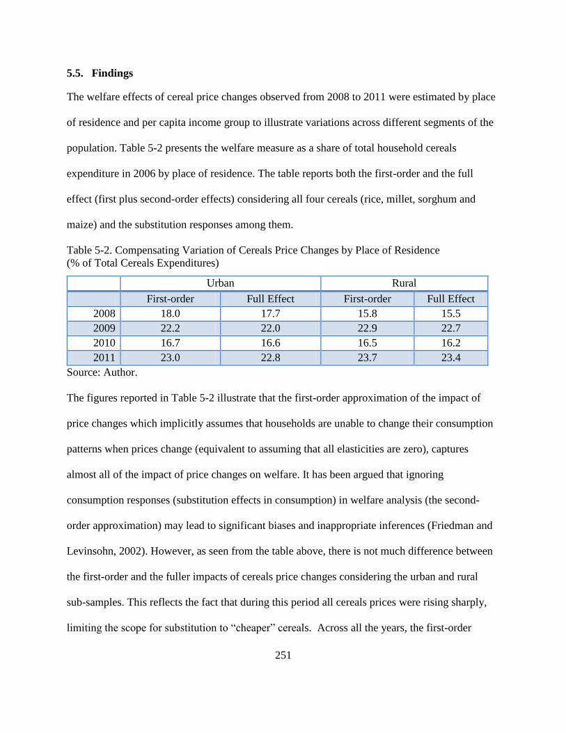
251
5.5. Findings
The welfare effects of cereal price changes observed from 2008 to 2011 were estimated by place
of residence and per capita income group to illustrate variations across different segments of the
population. Table 5-2 presents the welfare measure as a share of total household cereals
expenditure in 2006 by place of residence. The table reports both the first-order and the full
effect (first plus second-order effects) considering all four cereals (rice, millet, sorghum and
maize) and the substitution responses among them.
Table 5-2. Compensating Variation of Cereals Price Changes by Place of Residence
(% of Total Cereals Expenditures)
Urban Rural
First-order Full Effect First-order Full Effect
2008 18.0 17.7 15.8 15.5
2009 22.2 22.0 22.9 22.7
2010 16.7 16.6 16.5 16.2
2011 23.0 22.8 23.7 23.4
Source: Author.
The figures reported in Table 5-2 illustrate that the first-order approximation of the impact of
price changes which implicitly assumes that households are unable to change their consumption
patterns when prices change (equivalent to assuming that all elasticities are zero), captures
almost all of the impact of price changes on welfare. It has been argued that ignoring
consumption responses (substitution effects in consumption) in welfare analysis (the second-
order approximation) may lead to significant biases and inappropriate inferences (Friedman and
Levinsohn, 2002). However, as seen from the table above, there is not much difference between
the first-order and the fuller impacts of cereals price changes considering the urban and rural
sub-samples. This reflects the fact that during this period all cereals prices were rising sharply,
limiting the scope for substitution to “cheaper” cereals. Across all the years, the first-order
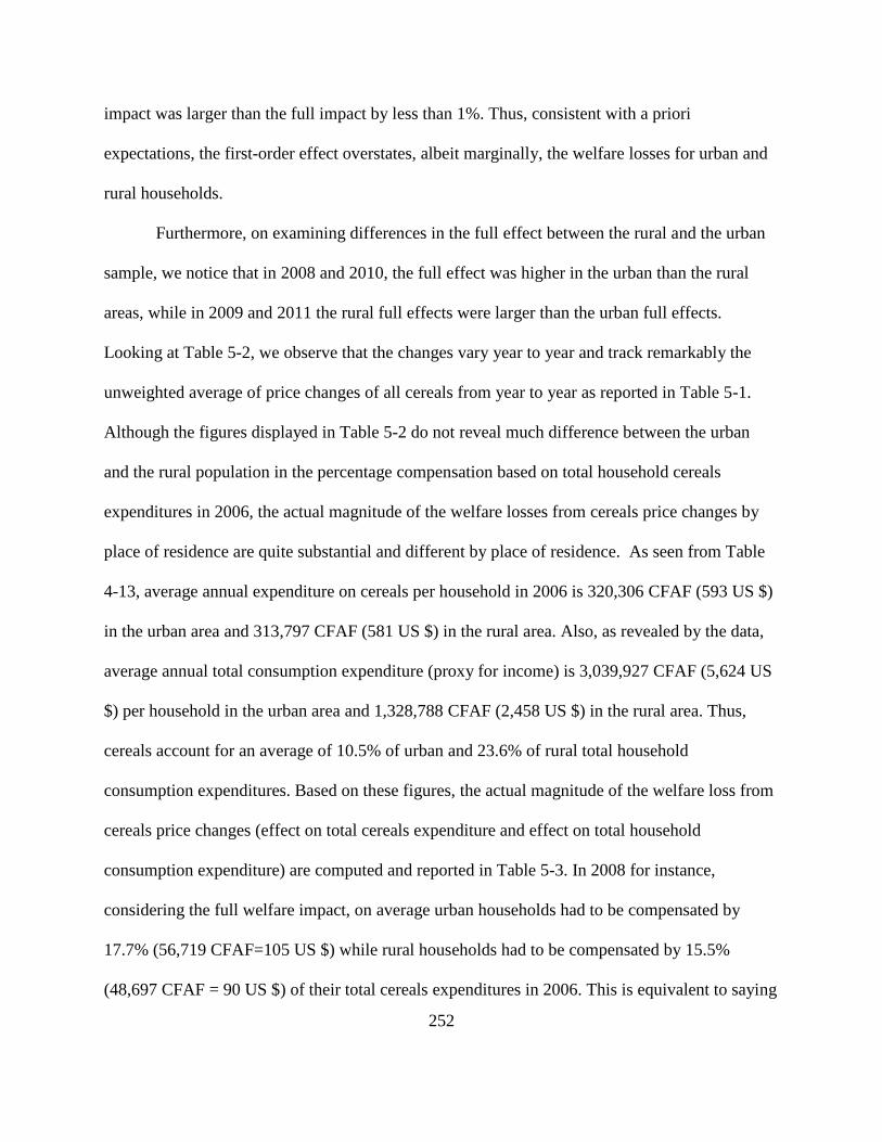
252
impact was larger than the full impact by less than 1%. Thus, consistent with a priori
expectations, the first-order effect overstates, albeit marginally, the welfare losses for urban and
rural households.
Furthermore, on examining differences in the full effect between the rural and the urban
sample, we notice that in 2008 and 2010, the full effect was higher in the urban than the rural
areas, while in 2009 and 2011 the rural full effects were larger than the urban full effects.
Looking at Table 5-2, we observe that the changes vary year to year and track remarkably the
unweighted average of price changes of all cereals from year to year as reported in Table 5-1.
Although the figures displayed in Table 5-2 do not reveal much difference between the urban
and the rural population in the percentage compensation based on total household cereals
expenditures in 2006, the actual magnitude of the welfare losses from cereals price changes by
place of residence are quite substantial and different by place of residence. As seen from Table
4-13, average annual expenditure on cereals per household in 2006 is 320,306 CFAF (593 US $)
in the urban area and 313,797 CFAF (581 US $) in the rural area. Also, as revealed by the data,
average annual total consumption expenditure (proxy for income) is 3,039,927 CFAF (5,624 US
$) per household in the urban area and 1,328,788 CFAF (2,458 US $) in the rural area. Thus,
cereals account for an average of 10.5% of urban and 23.6% of rural total household
consumption expenditures. Based on these figures, the actual magnitude of the welfare loss from
cereals price changes (effect on total cereals expenditure and effect on total household
consumption expenditure) are computed and reported in Table 5-3. In 2008 for instance,
considering the full welfare impact, on average urban households had to be compensated by
17.7% (56,719 CFAF=105 US $) while rural households had to be compensated by 15.5%
(48,697 CFAF = 90 US $) of their total cereals expenditures in 2006. This is equivalent to saying
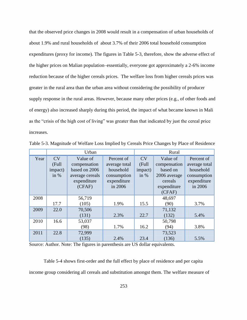
253
that the observed price changes in 2008 would result in a compensation of urban households of
about 1.9% and rural households of about 3.7% of their 2006 total household consumption
expenditures (proxy for income). The figures in Table 5-3, therefore, show the adverse effect of
the higher prices on Malian population–essentially, everyone got approximately a 2-6% income
reduction because of the higher cereals prices. The welfare loss from higher cereals prices was
greater in the rural area than the urban area without considering the possibility of producer
supply response in the rural areas. However, because many other prices (e.g., of other foods and
of energy) also increased sharply during this period, the impact of what became known in Mali
as the “crisis of the high cost of living” was greater than that indicated by just the cereal price
increases.
Table 5-3. Magnitude of Welfare Loss Implied by Cereals Price Changes by Place of Residence
Urban Rural
Year CV
(Full
impact)
in %
Value of
compensation
based on 2006
average cereals
expenditure
(CFAF)
Percent of
average total
household
consumption
expenditure
in 2006
CV
(Full
impact)
in %
Value of
compensation
based on
2006 average
cereals
expenditure
(CFAF)
Percent of
average total
household
consumption
expenditure
in 2006
2008
17.7
56,719
(105) 1.9% 15.5
48,697
(90) 3.7%
2009 22.0 70,506
(131) 2.3% 22.7
71,132
(132) 5.4%
2010 16.6 53,037
(98) 1.7% 16.2
50,798
(94) 3.8%
2011 22.8 72,999
(135) 2.4% 23.4
73,523
(136) 5.5%
Source: Author. Note: The figures in parenthesis are US dollar equivalents.
Table 5-4 shows first-order and the full effect by place of residence and per capita
income group considering all cereals and substitution amongst them. The welfare measure of
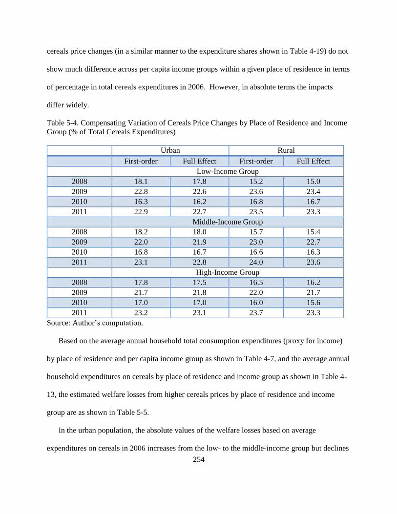
254
cereals price changes (in a similar manner to the expenditure shares shown in Table 4-19) do not
show much difference across per capita income groups within a given place of residence in terms
of percentage in total cereals expenditures in 2006. However, in absolute terms the impacts
differ widely.
Table 5-4. Compensating Variation of Cereals Price Changes by Place of Residence and Income
Group (% of Total Cereals Expenditures)
Urban Rural
First-order Full Effect First-order Full Effect
Low-Income Group
2008 18.1 17.8 15.2 15.0
2009 22.8 22.6 23.6 23.4
2010 16.3 16.2 16.8 16.7
2011 22.9 22.7 23.5 23.3
Middle-Income Group
2008 18.2 18.0 15.7 15.4
2009 22.0 21.9 23.0 22.7
2010 16.8 16.7 16.6 16.3
2011 23.1 22.8 24.0 23.6
High-Income Group
2008 17.8 17.5 16.5 16.2
2009 21.7 21.8 22.0 21.7
2010 17.0 17.0 16.0 15.6
2011 23.2 23.1 23.7 23.3
Source: Author’s computation.
Based on the average annual household total consumption expenditures (proxy for income)
by place of residence and per capita income group as shown in Table 4-7, and the average annual
household expenditures on cereals by place of residence and income group as shown in Table 4-
13, the estimated welfare losses from higher cereals prices by place of residence and income
group are as shown in Table 5-5.
In the urban population, the absolute values of the welfare losses based on average
expenditures on cereals in 2006 increases from the low- to the middle-income group but declines
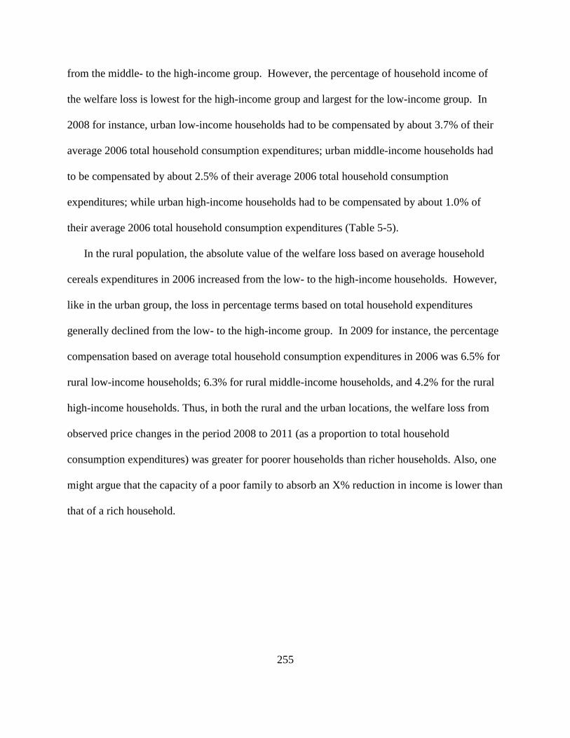
255
from the middle- to the high-income group. However, the percentage of household income of
the welfare loss is lowest for the high-income group and largest for the low-income group. In
2008 for instance, urban low-income households had to be compensated by about 3.7% of their
average 2006 total household consumption expenditures; urban middle-income households had
to be compensated by about 2.5% of their average 2006 total household consumption
expenditures; while urban high-income households had to be compensated by about 1.0% of
their average 2006 total household consumption expenditures (Table 5-5).
In the rural population, the absolute value of the welfare loss based on average household
cereals expenditures in 2006 increased from the low- to the high-income households. However,
like in the urban group, the loss in percentage terms based on total household expenditures
generally declined from the low- to the high-income group. In 2009 for instance, the percentage
compensation based on average total household consumption expenditures in 2006 was 6.5% for
rural low-income households; 6.3% for rural middle-income households, and 4.2% for the rural
high-income households. Thus, in both the rural and the urban locations, the welfare loss from
observed price changes in the period 2008 to 2011 (as a proportion to total household
consumption expenditures) was greater for poorer households than richer households. Also, one
might argue that the capacity of a poor family to absorb an X% reduction in income is lower than
that of a rich household.
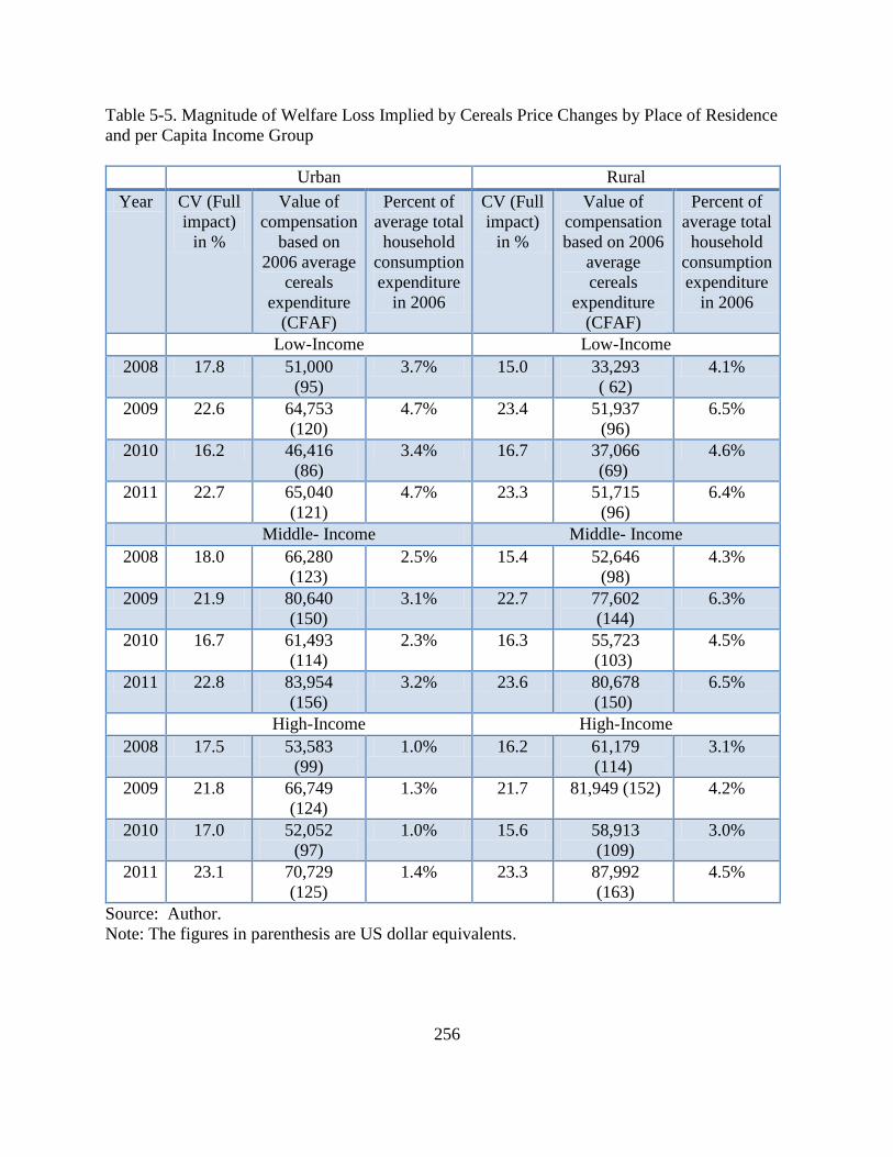
256
Table 5-5. Magnitude of Welfare Loss Implied by Cereals Price Changes by Place of Residence
and per Capita Income Group
Urban Rural
Year CV (Full
impact)
in %
Value of
compensation
based on
2006 average
cereals
expenditure
(CFAF)
Percent of
average total
household
consumption
expenditure
in 2006
CV (Full
impact)
in %
Value of
compensation
based on 2006
average
cereals
expenditure
(CFAF)
Percent of
average total
household
consumption
expenditure
in 2006
Low-Income Low-Income
2008 17.8 51,000
(95)
3.7% 15.0 33,293
( 62)
4.1%
2009 22.6 64,753
(120)
4.7% 23.4 51,937
(96)
6.5%
2010 16.2 46,416
(86)
3.4% 16.7 37,066
(69)
4.6%
2011 22.7 65,040
(121)
4.7% 23.3 51,715
(96)
6.4%
Middle- Income Middle- Income
2008 18.0 66,280
(123)
2.5% 15.4 52,646
(98)
4.3%
2009 21.9 80,640
(150)
3.1% 22.7 77,602
(144)
6.3%
2010 16.7 61,493
(114)
2.3% 16.3 55,723
(103)
4.5%
2011 22.8 83,954
(156)
3.2% 23.6 80,678
(150)
6.5%
High-Income High-Income
2008 17.5 53,583
(99)
1.0% 16.2 61,179
(114)
3.1%
2009 21.8 66,749
(124)
1.3% 21.7 81,949 (152) 4.2%
2010 17.0 52,052
(97)
1.0% 15.6 58,913
(109)
3.0%
2011 23.1 70,729
(125)
1.4% 23.3 87,992
(163)
4.5%
Source: Author.
Note: The figures in parenthesis are US dollar equivalents.
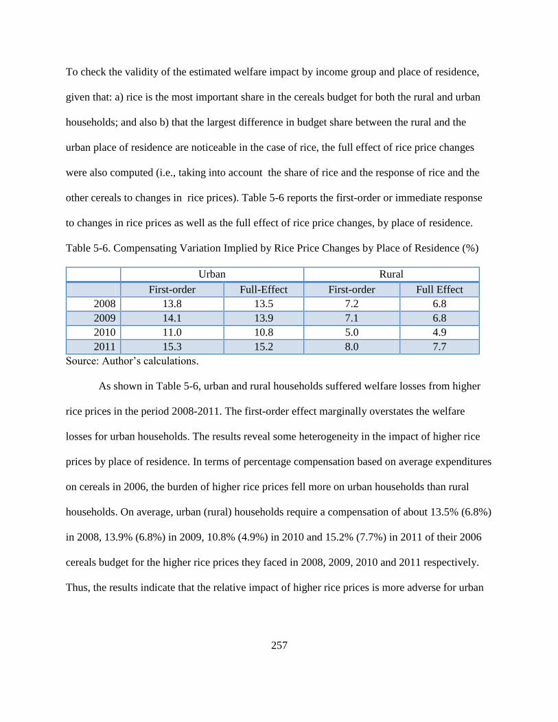
257
To check the validity of the estimated welfare impact by income group and place of residence,
given that: a) rice is the most important share in the cereals budget for both the rural and urban
households; and also b) that the largest difference in budget share between the rural and the
urban place of residence are noticeable in the case of rice, the full effect of rice price changes
were also computed (i.e., taking into account the share of rice and the response of rice and the
other cereals to changes in rice prices). Table 5-6 reports the first-order or immediate response
to changes in rice prices as well as the full effect of rice price changes, by place of residence.
Table 5-6. Compensating Variation Implied by Rice Price Changes by Place of Residence (%)
Urban Rural
First-order Full-Effect First-order Full Effect
2008 13.8 13.5 7.2 6.8
2009 14.1 13.9 7.1 6.8
2010 11.0 10.8 5.0 4.9
2011 15.3 15.2 8.0 7.7
Source: Author’s calculations.
As shown in Table 5-6, urban and rural households suffered welfare losses from higher
rice prices in the period 2008-2011. The first-order effect marginally overstates the welfare
losses for urban households. The results reveal some heterogeneity in the impact of higher rice
prices by place of residence. In terms of percentage compensation based on average expenditures
on cereals in 2006, the burden of higher rice prices fell more on urban households than rural
households. On average, urban (rural) households require a compensation of about 13.5% (6.8%)
in 2008, 13.9% (6.8%) in 2009, 10.8% (4.9%) in 2010 and 15.2% (7.7%) in 2011 of their 2006
cereals budget for the higher rice prices they faced in 2008, 2009, 2010 and 2011 respectively.
Thus, the results indicate that the relative impact of higher rice prices is more adverse for urban
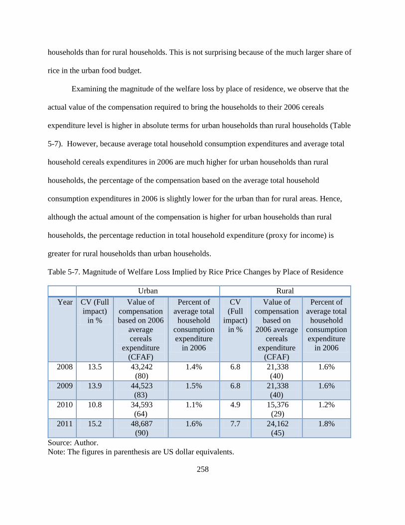
258
households than for rural households. This is not surprising because of the much larger share of
rice in the urban food budget.
Examining the magnitude of the welfare loss by place of residence, we observe that the
actual value of the compensation required to bring the households to their 2006 cereals
expenditure level is higher in absolute terms for urban households than rural households (Table
5-7). However, because average total household consumption expenditures and average total
household cereals expenditures in 2006 are much higher for urban households than rural
households, the percentage of the compensation based on the average total household
consumption expenditures in 2006 is slightly lower for the urban than for rural areas. Hence,
although the actual amount of the compensation is higher for urban households than rural
households, the percentage reduction in total household expenditure (proxy for income) is
greater for rural households than urban households.
Table 5-7. Magnitude of Welfare Loss Implied by Rice Price Changes by Place of Residence
Urban Rural
Year CV (Full
impact)
in %
Value of
compensation
based on 2006
average
cereals
expenditure
(CFAF)
Percent of
average total
household
consumption
expenditure
in 2006
CV
(Full
impact)
in %
Value of
compensation
based on
2006 average
cereals
expenditure
(CFAF)
Percent of
average total
household
consumption
expenditure
in 2006
2008 13.5 43,242
(80)
1.4% 6.8 21,338
(40)
1.6%
2009 13.9 44,523
(83)
1.5% 6.8 21,338
(40)
1.6%
2010 10.8 34,593
(64)
1.1% 4.9 15,376
(29)
1.2%
2011 15.2 48,687
(90)
1.6% 7.7 24,162
(45)
1.8%
Source: Author.
Note: The figures in parenthesis are US dollar equivalents.
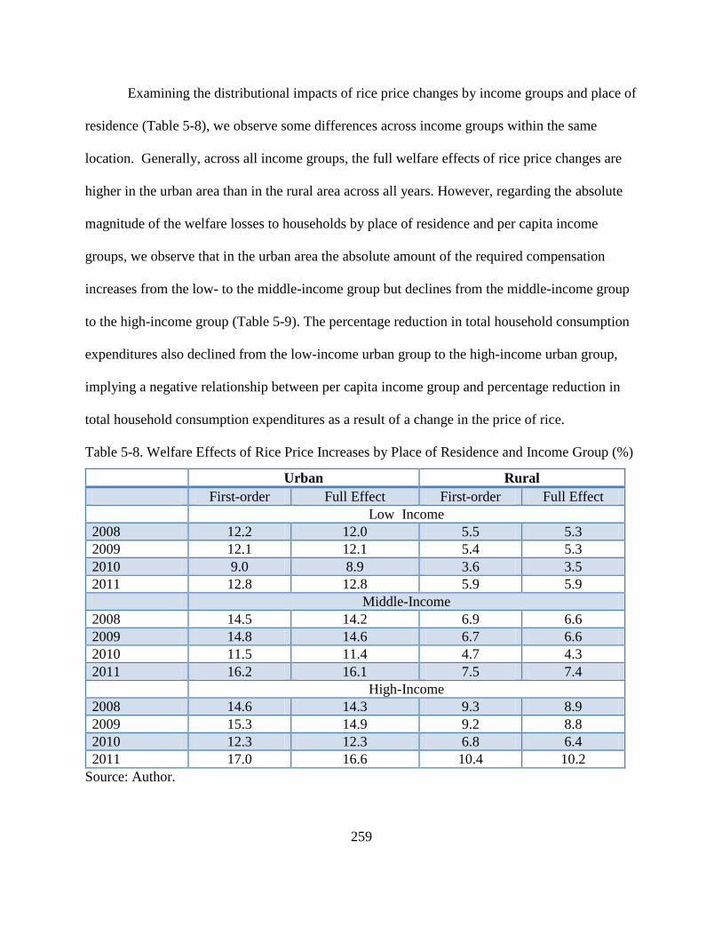
259
Examining the distributional impacts of rice price changes by income groups and place of
residence (Table 5-8), we observe some differences across income groups within the same
location. Generally, across all income groups, the full welfare effects of rice price changes are
higher in the urban area than in the rural area across all years. However, regarding the absolute
magnitude of the welfare losses to households by place of residence and per capita income
groups, we observe that in the urban area the absolute amount of the required compensation
increases from the low- to the middle-income group but declines from the middle-income group
to the high-income group (Table 5-9). The percentage reduction in total household consumption
expenditures also declined from the low-income urban group to the high-income urban group,
implying a negative relationship between per capita income group and percentage reduction in
total household consumption expenditures as a result of a change in the price of rice.
Table 5-8. Welfare Effects of Rice Price Increases by Place of Residence and Income Group (%)
Urban Rural
First-order Full Effect First-order Full Effect
Low Income
2008 12.2 12.0 5.5 5.3
2009 12.1 12.1 5.4 5.3
2010 9.0 8.9 3.6 3.5
2011 12.8 12.8 5.9 5.9
Middle-Income
2008 14.5 14.2 6.9 6.6
2009 14.8 14.6 6.7 6.6
2010 11.5 11.4 4.7 4.3
2011 16.2 16.1 7.5 7.4
High-Income
2008 14.6 14.3 9.3 8.9
2009 15.3 14.9 9.2 8.8
2010 12.3 12.3 6.8 6.4
2011 17.0 16.6 10.4 10.2
Source: Author.
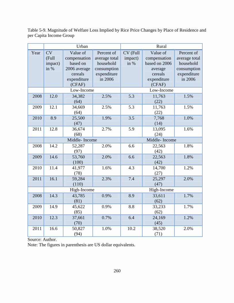
260
Table 5-9. Magnitude of Welfare Loss Implied by Rice Price Changes by Place of Residence and
per Capita Income Group
Urban Rural
Year CV
(Full
impact)
in %
Value of
compensation
based on
2006 average
cereals
expenditure
(CFAF)
Percent of
average total
household
consumption
expenditure
in 2006
CV (Full
impact)
in %
Value of
compensation
based on 2006
average
cereals
expenditure
(CFAF)
Percent of
average total
household
consumption
expenditure
in 2006
Low-Income Low-Income
2008 12.0 34,382
(64)
2.5% 5.3 11,763
(22)
1.5%
2009 12.1 34,669
(64)
2.5% 5.3 11,763
(22)
1.5%
2010 8.9 25,500
(47)
1.9% 3.5 7,768
(14)
1.0%
2011 12.8 36,674
(68)
2.7% 5.9 13,095
(24)
1.6%
Middle- Income Middle- Income
2008 14.2 52,287
(97)
2.0% 6.6 22,563
(42)
1.8%
2009 14.6 53,760
(100)
2.0% 6.6 22,563
(42)
1.8%
2010 11.4 41,977
(78)
1.6% 4.3 14,700
(27)
1.2%
2011 16.1 59,284
(110)
2.3% 7.4 25,297
(47)
2.0%
High-Income High-Income
2008 14.3 43,785
(81)
0.9% 8.9 33,611
(62)
1.7%
2009 14.9 45,622
(85)
0.9% 8.8 33,233
(62)
1.7%
2010 12.3 37,661
(70)
0.7% 6.4 24,169
(45)
1.2%
2011 16.6 50,827
(94)
1.0% 10.2 38,520
(71)
2.0%
Source: Author.
Note: The figures in parenthesis are US dollar equivalents.
261
Within the rural place of residence, we observe an increase in the percentage
compensation based on average total cereals expenditures in 2006 (full effect) required from rice
price changes as we move from the low- to the high-income groups. Additionally, we observe
that the actual magnitude of the compensation based on average expenditure on cereals in 2006
increases from the low- to the high-income rural population groups (Table 5-9).
In 2011 for instance, low-income rural households would need compensation of 13,095
CFAF (24 US $) to leave them indifferent to the price changes, the middle-income rural needed
compensation of 25,297 CFAF (47 US $), while the high-income rural population needed
compensation of 38,520 CFAF (71 US $). In terms of the percentage of the compensation in total
household consumption expenditures, the welfare losses were almost of the same magnitude in
the middle- and high-income rural population but lower in the low-income rural households.
Thus, the high- and middle-income rural households would have had to be compensated by a
slightly higher percentage of their total income following a change in the price of rice compared
to the low-income households to leave their welfare unaffected by the price hikes. The
explanation for this pattern is the increasing rice expenditure (Table 4-18) and expenditure shares
(Table 4-19) as rural households get richer.
Overall, we observe that all households are adversely affected by cereals price changes.
However, considering all four cereals and the substitution between them, there are not many
differences in the estimated full effects by place of residence and per capita income group in
terms of relative shares of the cereals budget. Although the actual value of the welfare loss as a
percentage of total household cereals expenditure in 2006 is higher amongst urban households
than rural household, the magnitude of the welfare loss based on the percentage of average total
household consumption expenditures were higher for rural households than urban households.
262
The analysis by place of residence shows that the adverse effect of the higher cereals prices on
Malian population ranged from a 1.7 to 5.5% income reduction, without considering the
possibility of producer supply response. Examining welfare losses by place of residence and per
capita income groups reveals that in the urban population the percentage reduction in total
household expenditure is lowest for the high-income group and largest for the low-income group.
In the rural population, the welfare loss in terms of percentage reduction in total household
expenditures in most cases declined from the low- to the high-income group.
Because of its importance in the Malian food basket in terms of consumption shares, rice
was isolated for the welfare impact evaluation to see whether there are any variations in welfare
effect by place of residence. The full effect of rice price changes revealed that rice accounts for a
substantial part of the overall welfare effect implied by higher cereals prices. Estimates of the
full effect of rice price changes taking into account rice consumption share and the response of
rice and other cereals to changes in rice prices show some heterogeneity in the impact of higher
rice prices by place of residence. In terms of percentage in the 2006 average total household
cereals budget, the burden of higher rice prices fell more on urban households than rural
households. This result was not surprising giving that the share of rice in cereals budget was
about 20% larger in the urban location than in the rural location. Examining the magnitude of the
welfare loss from higher rice prices by place of residence reveals that although the actual amount
of the compensation is higher for urban households than rural households, rural households
would have to be compensated by a greater percentage of the average of their 2006 total
household consumption expenditures than urban households.
Still considering the welfare effects of rice price changes only, we observe a general
increase in the full effect across per capita income groups within a particular place of residence
263
in terms of relative shares in the cereals budget. The distributional impacts of higher rice prices
by income group and place of residence reveal a decline in the percentage income reduction from
the low- to the high-income urban group. In the rural population, the reductions in total
household expenditures emanating from higher rice prices are quite similar in the middle- and
high-income group, but smaller in the low-income rural group. The increasing in welfare loss (in
terms of percentage in total household expenditures) from a change in the price of rice from the
rural low- to the rural high-income group reflects increasing rice expenditure and rice
expenditure shares with growth in rural per capita income.
264
CHAPTER 6. SUMMARY OF MAJOR FINDINGS AND IMPLICATIONS FOR THE
FOOD SECURITY POLICIES IN MALI
6.1. Summary of Major Findings and Policy Implications
The goal of this study was to examine trends and determinants of food consumption patterns in
West Africa and draw some implications for the design of food security policies. Knowledge of
food demand parameters and of how consumption patterns have changed over time is critical for
informed food policy making. However, in WA, information on food demand parameters is
limited, thus restricting policymakers’ ability to make sound food policy decisions. One ultimate
goal of the analysis of food consumption patterns is to improve the efficiency of government
interventions by providing policymakers, for example, with suggestions for the design of food
security policies compatible with targeting people based on the nature and extent of food
insecurity.
As defined by FAO (2006), “Food security exists when all people, at all times, have
physical and economic access to sufficient, safe and nutritious food that meets their dietary needs
and food preferences for an active and healthy life”. Food security is a broad concept which cuts
across many dimensions. The four main dimensions of food security extracted from this
definition are: sufficient quantities available for consumption, sustained access to food by each
individual (adequate resources to obtain appropriate foods for a nutritious diet), effective
utilization, and stable food supply (FAO, 2006). Simply put, people are food insecure when they
do not “eat right” due to a lack of either physical or monetary access to food. Diaz-Bonilla et al.
(2000) also observe that while food availability and access are preconditions for adequate
utilization, they do not determine unequivocally the more substantive issue of malnutrition and
265
nutrition security at the individual level. Furthermore, from an economist’s point of view, access
to food depends on income, prices, and distance to local food markets.
Chapter 2 in this study explores physical food sufficiency, measured through aggregate-
level food supply indicators. Specifically, the chapter analyzes aggregate-level trends in per
capita food availability in the ECOWAS countries of West Africa using a descriptive approach
and per capita food availability data from FAO’s FBS covering the period 1980-2009. With
respect to the aggregate-level trend in per capita daily energy availability (DEA), the analysis
reveals: 1) an overall pattern of shift towards greater calorie availability in the region; 2) a
remarkably positive growth in per capita DEA over time amongst the countries that have
experienced strong economic performance, like Ghana and Nigeria; and 3) less favorable trends
in per capita DEA in countries that have experienced civil disruption, like Liberia, Sierra Leone
and Cote d’Ivoire. Per capita DEA has been widely used in the literature as one of the main
determinants of national food availability (Smith and Haddad, 2000). As a national average,
DEA is sometimes viewed as an imperfect indicator of the state of individual food security.
However, empirical evidence, such as that provided by Smith and Haddad (2000), suggest that
there is a strong correlation between this per capita DEA and more individual-based indicators of
food security (e.g., anthropometric indicators of children’s nutritional status). In particular, Smith
and Haddad (2000) show that national caloric availability was responsible for more than a
quarter of reductions in child malnutrition in developing countries over the period 1970-95.
Consequently, based on the observed trend in per capita DEA in the current study, one can say
that there have been some improvements in the state of food security over the last three decades.
The analysis of the trend in the composition of food supply over time provides evidence
of a diversification in the composition of food supply. Starchy roots and tubers are emerging as
266
important contributors to the diets. In the Sahel for instance, we observe growth in percentage
terms in starchy R&T availability per capita. However, this has been from a small base. The
growth in the supply of starchy R&T has been greatest along the humid coast of WA. In some
Coastal Non-Sahelian countries (Nigeria, Ghana, and Sierra Leone) there has been a big cassava
revolution. The apparent per capita consumption of cassava grew in Senegal; that of sweet
potatoes grew in Mali; and that of yams also showed huge increases in some Coastal Non-
Sahelian countries (e.g., Ghana and Nigeria). The supply of Irish potatoes grew in some
countries (e.g., Cape Verde and Senegal), while that of maize showed a striking growth in the
Sahel (Burkina Faso, Mali and Senegal). Apparent per capita rice consumption increased for
most countries in the study period. In Cape Verde for instance, there has been a replacement of
maize with rice as the dominant type of cereal. These findings therefore present a scope to
encourage ongoing diversification of staple food sources to give consumers more opportunity for
substitution and choice.
Not only have there been greater per capita availability of food and a diversification in
the composition of the diet, but also the quality of food available has improved over time in
terms of major macronutrient composition. Daily protein supply per capita has grown for most
countries since the early 2000s. This study goes beyond examining the average per capita levels
of total protein availability to disaggregate per capita protein availability by source. Protein
quality varies by source, and animal proteins are generally of higher quality (essential amino
acids) than protein from plant sources. Diaz-Bonilla et al. (2000) suggest that the availability of
animal proteins is more directly correlated with measures of nutritional security than is the
availability of total proteins. Animal protein supply has been increasing for some countries in the
region. The growth in the supply of animal protein reflects greater purchasing power (effective
267
demand). In countries that have experienced rapid economic growth over time like Ghana and
Cape Verde, the growth in the supply of animal protein has been remarkable. Countries with
modest economic growth, such as Mali, have also shown modest growth in the consumption of
animal protein over time. Decomposing animal protein by specific source, it is observed that
growth in the apparent per capita consumption of poultry meat has been quite large for most
countries in the region, although fish remains the dominant source of animal protein for most
coastal countries.
Furthermore, while plant protein dominates as the major source of protein for most
countries in the region, some of these countries (e.g., Niger, Sierra Leone, Nigeria and Cape
Verde) derive an important share of vegetable protein from pulses, which are also a source of
high-quality protein. The positive growth in protein supply from pulses as well as in the share of
pulses in daily vegetable protein supply supports the emergence of pulses as poor people’s meat
in the region. This finding provides a scope to encourage and promote agricultural practices like
crop rotation or intercropping of cereals with high protein grain legumes. Such agronomic
practices will not only enhance soil fertility in an era of rising prices of inorganic fertilizers and
climate change, but will also present an alternative to expensive animal protein, particularly for
low-income households. Growth in the consumption of high quality plant protein would result in
improvement in the nutritional status of poor households who cannot afford the expensive animal
protein. Apparent per capita daily fat supply increased for most countries in the study period.
There has therefore been some diet upgrading as the consumption of important macronutrients
such as fats and protein have increased in the last three decades.
The analysis of aggregate-level determinants of starchy staples demand (Chapter 3) after
correcting for the unit roots properties of the data does not support any statistical association
268
between the urban population share and cereals consumption behavior in Senegal, but points to a
statistically significant negative relationship between millet and urban population share in Mali.
Evidence on the role of per capita income in influencing cereals consumption at the aggregate
level reveals a statistically significant relationship between per capita cereals budget and rice and
millet expenditure shares in the dynamic demand specification in Mali. The analysis also reveals
no evidence in support of a statistical association between per capita income and starchy staples
consumption in Senegal.
The Hicksian cross-price elasticities from the error-corrected demand model provide
evidence of a relationship of substitution in the short-run and long-run between rice and sorghum
as hypothesized for Mali and Senegal. Furthermore for Mali, maize is found to be a substitute for
rice and sorghum. In Benin, we observe\ a relationship of substitution between maize and yams
in the short-run–both are used to make “fufu”, a basic carbohydrate main dish eaten with sauce.
An implication of these statistically significant relationships of substitution is that they offer a
scope to encourage ongoing diversification of starchy staples consumption, thereby giving
consumers more opportunities for substitution and choices.
Micro-level analysis in Chapter 4 gives us a closer look into the situation of food security
at the household level. Using Mali’s 2006 HBS data, households’ economic access to food
(measured by the household’s food expenditures) is examined alongside other factors at the
household level to understand household food consumption behavior. Effective design of
targeted actions requires knowledge of the distribution of the effects of changes in income as
well as factors other than income that determine food demand — e.g., food prices and place of
residence. To understand differences in cereals consumption by per capita income group, the
rural and urban subsamples were each divided separately in thirds and households were assigned
269
to high, medium, and low-income groups for each type of residence, and demand parameters
were estimated for each group. The demand for cereals is specified as a QUAIDS model which
takes care of common problems in household demand estimation such as zero-expenditure and
endogeneity in total cereals expenditure.
The analysis in Chapter 4 reveals high expenditure elasticities for starchy staples. In
particular, in the urban area, rice expenditure elasticity seems to have increased over time while
the expenditure elasticity of sorghum is very high. With past findings that coarse grains are
generally less preferred in the urban areas for various reasons such as the high opportunity cost
of the time required for their preparation, the high sorghum expenditure elasticity warrants an
investigation of consumer preferences for sorghum with different quality attributes. In the rural
area, rice and millet are also high in expenditure elasticity. The high expenditure elasticities even
for staples suggest strong future growth in demand and hence pressure on prices if supply is not
increased. Therefore, the need to focus on driving down unit costs throughout the food system.
Expenditure elasticities disaggregated by income-group and place of residence also reveal
rice demand to increase in expenditure elasticity from the low- to the high-income urban groups.
Millet and sorghum, on the other hand, become less preferred as urban households get richer, and
the high expenditure elasticity obtained when all urban households are combined appears to be
largely driven by the behavior of low-income urban households. In the rural areas, all four
cereals increase in expenditure elasticity as households get richer.
The findings of this study also provide scope to encourage ongoing diversification of
staple food sources to give consumers more opportunity for substitution and choice. Sorghum
demand was found to be the most responsive to own-price changes in the urban area. Also,
disaggregating by income group, the demand for sorghum is most sensitive amongst the high
270
income urban group. If the high own-price elasticity of sorghum estimated represents urban
Malian consumer behavior correctly, efforts geared towards expanding sorghum production and
driving down the unit cost of production could encourage the consumption of sorghum
Furthermore, the analysis reveals that for the range of prices observed in 2006, the price
of rice appears to have a significant effect on the consumption of coarse grains in the urban area,
whereby sorghum and millet are substitutes for rice. Thus, in the event of high rice prices, the
consumption of traditional coarse grains in the urban areas can be encouraged by promoting the
production of coarse grains (increased availability), and also by encouraging private sector
involvement in the processing of these coarse grains to reduce preparation time. Further research
can be carried out to investigate consumers’ preference for cereals with different quality
attributes. Disaggregated across income groups and place of residence, the compensated cross-
price elasticities point mostly to a relationship of substitution between the different cereals. This
reveals not only a scope for dealing with price spikes for one cereal by increasing the availability
of substitutes—a possibility that the earlier findings of low cross-price elasticities seemed to
discount, but also a scope for price transmission across cereals across cereals. Thus, there is
need for a cereals policy rather than just, for example, a rice policy.
The welfare analysis of cereals price shocks in Mali over the period 2008-2011, taking
into account the first order-response and the substitution responses, reveals not very large
substitution effect for the reason that all cereals prices rose together. Estimates of the full impact
reveal that all households are adversely affected by cereals price changes and the adverse effect
of the higher cereals prices on Malian population ranged from a 2 to 6% income reduction,
without considering the possibility of producer supply response. Disaggregating across income
groups, the analysis reveals that in both the urban and rural population, low-income households
271
are hardest hit by cereals price increases–i.e., the percentage reduction in total household
expenditure is lowest for the high-income group and largest for the low-income group. The
decreasing expenditure elasticity of sorghum and millet as per capita income increase (discussed
above), particularly in the urban area, and the willingness to substitute one cereal type for
another implies that expanding the availability of these cereals could help reduce some of the
welfare losses from cereals price shocks. The welfare losses from the recent price hikes imply a
need to address supply (including marketing and processing) issues due to concerns about
welfare and food security, as well as the likely impacts on economic growth of a likely reduced
consumer spending on non-food items.
6.2. Limitations of the Study
Despite the limitations outlined throughout the study, we can say that the key objectives of the
study have been met in their essence. Yet, this study could be improved in many respects.
Ideally, the analysis of household level food demand in a developing economy like that of Mali
that has the rural population producing most of the food consumed in the country should go
beyond measuring just consumption responses to measuring producer supply response to food
price changes as well. Under the perspective of an agricultural household model, consumption
behavior is complicated by production decisions. While most urban households are solely food
consumers, most rural households are also food producers, such that changes in food prices
affect them as consumers and producers. Furthermore, an increase in the price of a food
commodity could increase the demand for that commodity (contrary to traditional demand
theory) since a farmer may produce more of it and gain more income. Consequently, the net
welfare effect of a price change depends on whether the household is a net-seller or net buyer of
272
food. Net food-selling households may see an increase in income that may compensate for the
rise in the price of foods they purchase, while the net food-buying households are likely to be
adversely affected by increases in the prices of foods they purchase. Unfortunately, as a result of
data limitations, the analyses of cereals demand and the welfare effect of cereals price shocks in
this study fails to account for the production or additional profit effect for food producing
households that could accompany rising food prices. To carry out such analysis, one would need
data on production by cereal type, production shares by cereal types, as well as input and output
prices.
Consumption patterns are determined by a combination of three factors: level of income,
the preferences of households, and market prices. Preferences are in turn affected by the
composition of the household, its members’ knowledge and education, habits and cultural norms,
biological factors that affect hunger, etc. (Ruel et al. 2005). Two key assumptions of standard
household demand models are that household resources are pooled and that the household has a
single set of preferences. In the modeling of household cereals consumption behavior, the
current study does not take into account differences in preferences within a household and in the
intra-household allocation of resources and especially food. While it is recognized here that there
are significant gender dimensions to the challenge of ensuring food security, in the absence of
sex-disaggregated data it is hard to investigate any gender differences in the allocation of
household production and consumption resources, and also in the availability and utilization of
food within a household, making it even harder to understand any gender differences in the
welfare effects of food price increases.

273
BIBLIOGRAPHY
274
BIBLIOGRAPHY
Aksoy, M.A. and Hoekman, B. 2010. Food Prices and Rural Poverty. Centre for Economic
Policy Research and the World Bank, Introduction and Overview. Accessed at
http://siteresources.worldbank.org/INTRANETTRADE/Resources/Pubs/Food_Prices_Ru
ral_Poverty.pdf 3, 6, 7, 25
Alderman, H. 1986.The Effect of Food Price and Income Changes on the Acquisition of Food
by Low-Income Households. Washington DC: International Food Policy Research
Institute, 1986.
Alfonzo, L. and Peterson, H. H. 2006. “Estimating food demand in Paraguay from household
Survey data”. Agricultural Economics, 34: 243–257.
Alpay, S. and Koc, A.2002. Household Demand in Turkey: an Application of Almost Ideal
Demand System with Spatial Cost Index. Economic Research Forum Volume 226 of
Working paper.
Alviola, P. A., IV, Capps, O., Jr. and Wu, X. 2010. Micro-Demand Systems Analysis of Non-
Alcoholic in the United States. An Application of Econometric Techniques Dealing with
Censoring. Agricultural and Applied Economics Association>2010 Annual Meeting, July
25-27, 2010, Denver, Colorado. URL: http://purl.umn.edu/60462
Asche F. and Wessels C.R. 1997. On Price Indices in the Almost Ideal Demand System.
American Journal of Agricultural Economics 79:1182–1185.
Balcombe, K.G., and Davis, J.R., 1996. An Application of Cointegration Theory in the
Estimation of the Almost Ideal Demand System for Food Consumption in Bulgaria.
Agric. Econ. 15, 47–60.
Banks, J., R. Blundell and A. Lewbel. 1997. “Quadratic Engel Curves and Consumer Demand.”
Review of Economics and Statistics 79 (1997): 527-539.
Barslund, N. 2011."Censored Demand System Estimation with Endogenous Expenditures in
Clustered samples: an application to food demand in urban Mozambique," LICOS
Discussion Papers 28011, LICOS - Centre for Institutions and Economic Performance,
K.U.Leuven. File URL: http://www.econ.kuleuven.be/licos/DP/DP2011/DP280.pdf
Blundell, R. and M. Robin. 1999. “Estimation in Large and Disaggregated Demand Systems: An
Estimator for Conditionally Linear Systems.” Journal of Applied Econometrics 14
(1999): 209-232.
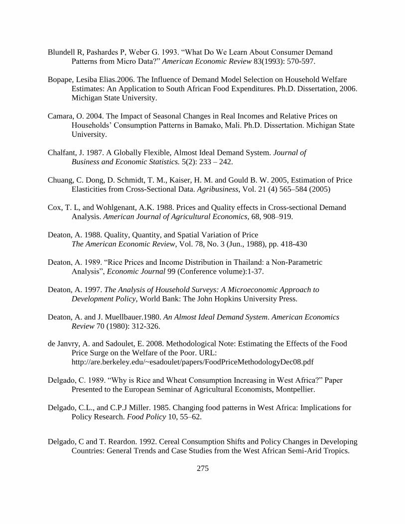
275
Blundell R, Pashardes P, Weber G. 1993. “What Do We Learn About Consumer Demand
Patterns from Micro Data?” American Economic Review 83(1993): 570-597.
Bopape, Lesiba Elias.2006. The Influence of Demand Model Selection on Household Welfare
Estimates: An Application to South African Food Expenditures. Ph.D. Dissertation, 2006.
Michigan State University.
Camara, O. 2004. The Impact of Seasonal Changes in Real Incomes and Relative Prices on
Households’ Consumption Patterns in Bamako, Mali. Ph.D. Dissertation. Michigan State
University.
Chalfant, J. 1987. A Globally Flexible, Almost Ideal Demand System. Journal of
Business and Economic Statistics. 5(2): 233 – 242.
Chuang, C. Dong, D. Schmidt, T. M., Kaiser, H. M. and Gould B. W. 2005, Estimation of Price
Elasticities from Cross-Sectional Data. Agribusiness, Vol. 21 (4) 565–584 (2005)
Cox, T. L, and Wohlgenant, A.K. 1988. Prices and Quality effects in Cross-sectional Demand
Analysis. American Journal of Agricultural Economics, 68, 908–919.
Deaton, A. 1988. Quality, Quantity, and Spatial Variation of Price
The American Economic Review, Vol. 78, No. 3 (Jun., 1988), pp. 418-430
Deaton, A. 1989. “Rice Prices and Income Distribution in Thailand: a Non-Parametric
Analysis”, Economic Journal 99 (Conference volume):1-37.
Deaton, A. 1997. The Analysis of Household Surveys: A Microeconomic Approach to
Development Policy, World Bank: The John Hopkins University Press.
Deaton, A. and J. Muellbauer.1980. An Almost Ideal Demand System. American Economics
Review 70 (1980): 312-326.
de Janvry, A. and Sadoulet, E. 2008. Methodological Note: Estimating the Effects of the Food
Price Surge on the Welfare of the Poor. URL:
http://are.berkeley.edu/~esadoulet/papers/FoodPriceMethodologyDec08.pdf
Delgado, C. 1989. “Why is Rice and Wheat Consumption Increasing in West Africa?” Paper
Presented to the European Seminar of Agricultural Economists, Montpellier.
Delgado, C.L., and C.P.J Miller. 1985. Changing food patterns in West Africa: Implications for
Policy Research. Food Policy 10, 55–62.
Delgado, C and T. Reardon. 1992. Cereal Consumption Shifts and Policy Changes in Developing
Countries: General Trends and Case Studies from the West African Semi-Arid Tropics.
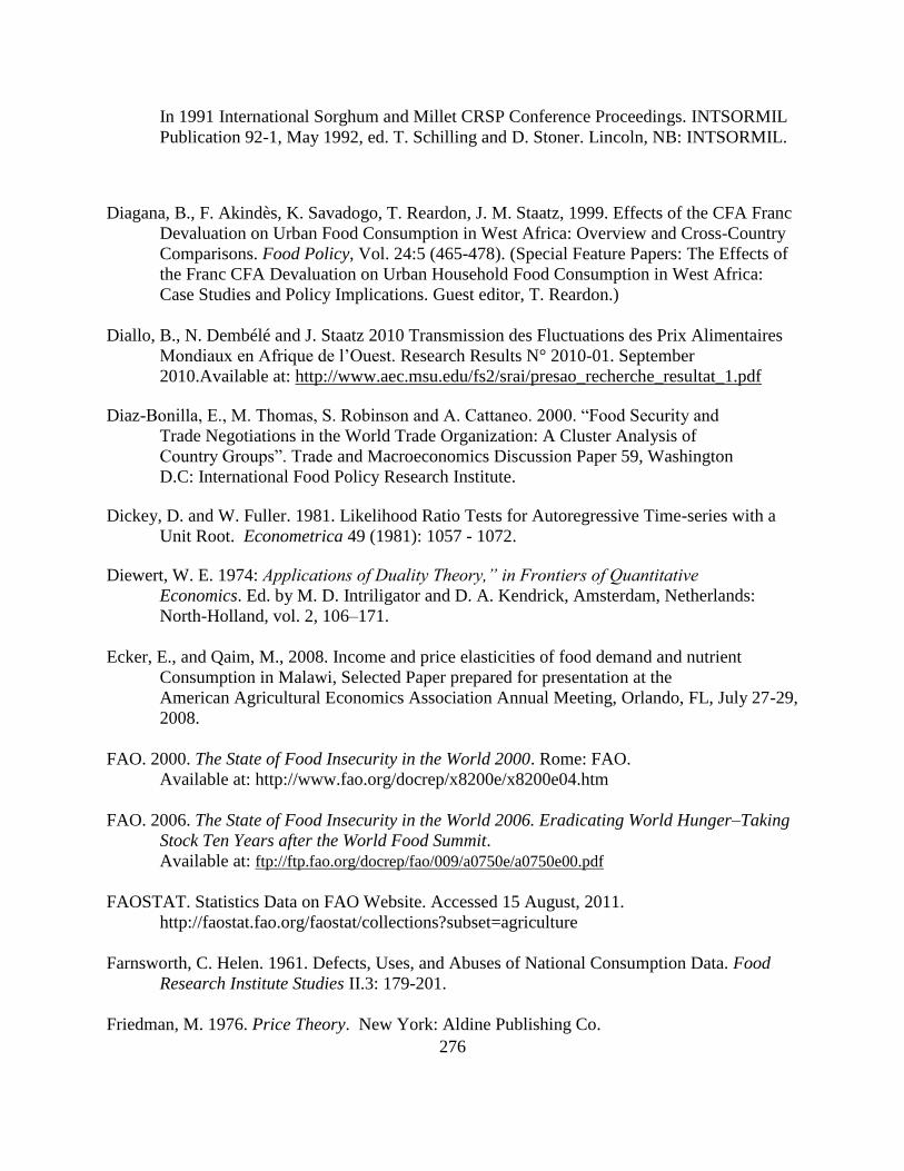
276
In 1991 International Sorghum and Millet CRSP Conference Proceedings. INTSORMIL
Publication 92-1, May 1992, ed. T. Schilling and D. Stoner. Lincoln, NB: INTSORMIL.
Diagana, B., F. Akindès, K. Savadogo, T. Reardon, J. M. Staatz, 1999. Effects of the CFA Franc
Devaluation on Urban Food Consumption in West Africa: Overview and Cross-Country
Comparisons. Food Policy, Vol. 24:5 (465-478). (Special Feature Papers: The Effects of
the Franc CFA Devaluation on Urban Household Food Consumption in West Africa:
Case Studies and Policy Implications. Guest editor, T. Reardon.)
Diallo, B., N. Dembélé and J. Staatz 2010 Transmission des Fluctuations des Prix Alimentaires
Mondiaux en Afrique de l’Ouest. Research Results N° 2010-01. September
2010.Available at: http://www.aec.msu.edu/fs2/srai/presao_recherche_resultat_1.pdf
Diaz-Bonilla, E., M. Thomas, S. Robinson and A. Cattaneo. 2000. “Food Security and
Trade Negotiations in the World Trade Organization: A Cluster Analysis of
Country Groups”. Trade and Macroeconomics Discussion Paper 59, Washington
D.C: International Food Policy Research Institute.
Dickey, D. and W. Fuller. 1981. Likelihood Ratio Tests for Autoregressive Time-series with a
Unit Root. Econometrica 49 (1981): 1057 - 1072.
Diewert, W. E. 1974: Applications of Duality Theory,” in Frontiers of Quantitative
Economics. Ed. by M. D. Intriligator and D. A. Kendrick, Amsterdam, Netherlands:
North-Holland, vol. 2, 106–171.
Ecker, E., and Qaim, M., 2008. Income and price elasticities of food demand and nutrient
Consumption in Malawi, Selected Paper prepared for presentation at the
American Agricultural Economics Association Annual Meeting, Orlando, FL, July 27-29,
2008.
FAO. 2000. The State of Food Insecurity in the World 2000. Rome: FAO.
Available at: http://www.fao.org/docrep/x8200e/x8200e04.htm
FAO. 2006. The State of Food Insecurity in the World 2006. Eradicating World Hunger–Taking
Stock Ten Years after the World Food Summit.
Available at: ftp://ftp.fao.org/docrep/fao/009/a0750e/a0750e00.pdf
FAOSTAT. Statistics Data on FAO Website. Accessed 15 August, 2011.
http://faostat.fao.org/faostat/collections?subset=agriculture
Farnsworth, C. Helen. 1961. Defects, Uses, and Abuses of National Consumption Data. Food
Research Institute Studies II.3: 179-201.
Friedman, M. 1976. Price Theory. New York: Aldine Publishing Co.
277
Friedman, J. and Levinsohn, J.A. 2002, “The Distributional Impact of Indonesia’s
Financial Crisis on Household Welfare: A ‘Rapid Response’ Methodology”, World
Bank Economic Review, vol. 16, no. 3, pp. 397-423.
Gossen, F. 2002. Potato Marketing in Rwanda. Prepared for United States Agency for
International Development/Rwanda.
http://pdf.usaid.gov/pdf_docs/pnacx568.pdf
Hausman, J.A., 1978. Specification tests in econometrics‟. Econometrica 46, pp. 931-959.
Heckman, J. 1978. Dummy endogenous variables in a simultaneous equation system.
Econometrica, 46: 931-959.
Heien, D. and Wessells, C. 1990. Demand Systems Estimation with Microdata: a Censored
Regression Approach. Journal of Business and Economic Statistics, 8(3): 365-371.
Ivanic, M. and W. Martin. 2008. “Implications of higher global food prices for poverty in low-
Income countries.” Policy Research Working Paper 4594.The World Bank, Washington,
DC. Available at SSRN: http://ssrn.com/abstract=1149097
Joseph, George and Wodon, Quentin, 2008."Assessing the potential impact on poverty of Rising
Cereals Prices: the Case of Mali," Policy Research Working Paper Series 4744, The
World Bank. Downloadable at http://ideas.repec.org/s/wbk/wbrwps.html
Karagiannis, G., S. Katranidis, and K. Velentzas 2000: “An Error Correction Almost Ideal
Demand System for Meat in Greece,” Agricultural Economics, 22, 29–35.
Kelly, V., N. Dembele, J. Staatz. 2008. Potential Food Security Impacts of Rising Commodity
Prices in the Sahel: 2008-2009: A special report by the Famine Early Warning Systems
Network. Washington, D.C.: FEWS NET
Kelly, V. N., Murekezi, A., Me-Nsope, N.M., Perakis, A. and Mather, D. 2012. Cereal Market
Dynamics: The Malian Experience from the 1990s to Present. MSU International
Development Working Paper (IDWP) No. 128. December 2012.
Available at: http://aec.msu.edu/fs2/papers/idwp.htm
Kennedy, E and T. Reardon. 1994. Shift to Non-traditional Grains in the Diets of East and West
Africa: Role of Women’s Opportunity Cost of Time. Food Policy 19 (1) 45-56
Kwiatkowski D., P. C. B. Phillips, P. Schmidt, and Y. Shin. 1992. Testing the Null Hypothesis of
Stationarity against the Alternative of a Unit Root: How Sure Are We that Economic
Time-series Have a Unit Root? Journal of Econometrics 54 (1992): 159 - 178.
278
Lele, U. M. and Mellor, J. W. 1972. Jobs, Poverty and the "Green Revolution".
International Affairs (Royal Institute of International Affairs 1944) Vol. 48, No. 1, pp.
20-32
Lopriore, C. and E. Muehlhoff. 2003. Food Security and Nutrition Trends in West Africa -
Challenges and the Way Forward. Presented at the 2nd International Workshop Food-
based Approaches for a Healthy Nutrition, 23-28 November, 2003. Ouagadougou,
Burkina Faso. Available at: http://www.mpl.ird.fr/fn2ouaga/P2IW_Part%201.pdf
Me-Nsope, N. M. and Staatz, J. M. 2013. Trends and Determinants of Food Consumption
Patterns in West Africa. Michigan State University. International Development Working
Paper. February 2013.
Mghenyi, E., Myers, R. J. and Jayne, T.S. 2011. The Effects of a Large Discrete Maize Price
Increase on the Distribution of Household Welfare and Poverty in Rural Kenya.
Agricultural Economics, 42: 343–356. doi: 10.1111/j.1574-0862.2010.00518.x
Minot, N. 2010. Transmission of World Food Price Changes to African Markets and its Effect on
Household Welfare” Paper to be presented at the COMESA policy seminar “Food price
Variability: Causes, consequences, and policy options”. On 25-26 January 2010 in
Maputo, Mozambique under the COMESA-MSU-IFPRI African Agricultural Markets
Project (AAMP)
Available at: citeseerx.ist.psu.edu/viewdoc/download?doi=10.1.1.193.5743...
Moschini, G. 1995: Units of Measurement and the Stone Index in Demand System Estimation.
American Journal of Agricultural Economics, 77, 63–68.
Muellbauer, J. 1976. Community Preferences and the Representative Consumer. Econometrica,
Vol. 44, No. 5. (Sep., 1976), pp. 979-999.
Nishida, C., R. Uauy, S. Kumanyika, and P. Shetty. 2004. The Joint WHO/FAO Expert
Consultation on Diet, Nutrition, and the Prevention of Chronic Diseases: Process,
Product, and Policy Implications. Public Health Nutrition 7.1A: 245–50.
Nouve, Kofi, and Quentin Wodon 2008. “Impact of Rising Rice Prices and Policy Response in
Mali: Simulations with Dynamic CGE Model.” Mimeo, World Bank, Washington, DC.
Nweke, F.I., D.S.C. Spencer, and J.K. Lynam. 2002. The Cassava Transformation: Africa's Best
Kept Secret. East Lansing: Michigan State University Press.
Nzuma, J.M. and Sarker, R. 2008. An Error Corrected Almost Ideal Demand System for Major
Cereals in Kenya. Selected Paper prepared for presentation at the American Agricultural
Economics Association Annual Meeting, Orlando, Florida, and July 27-29, 2008.
279
Phillips, P. and P. Perron.1988. Testing for a Unit Root in Time-series Regression. Biometrika
75: 335 - 346.
Poi, B. P. 2008. “Demand System Estimation: Update,” The Stata Journal, 2 (4), 554-556.
Pollak, R. A. and Wales T. J. 1987. Pooling International Consumption Data. The Review of
Economics and Statistics, Vol. 69, No. 1 (Feb., 1987), pp. 90-99
Porto Guido G. 2005, “Informal Export Barriers and Poverty”, Journal of International
Economics, 66, 447–70.
Porto, G. G., 2010. Food Prices and Rural Poverty. Centre for Economic Policy Research and
The World Bank, Ch. Food Prices: Household Responses and Spillover, pp. 167–184.
URL http://siteresources.worldbank.org/INTRANETTRADE/
Resources/Pubs/Food_Prices_Rural_Poverty.pdf 3, 6, 7, 25
Prais, S., and Houthakker, H. 1955. The Analysis of Family Budgets. Cambridge University
Press, Cambridge, 2nd ed. 1972 edn.
Reardon, T., T. Thiombiano and C. Delgado. 1988. “Substitution of Imported for Traditional
Cereals in Household Food Consumption in Ouagadougou, Burkina Faso”. IFPRI
Research Report.
Regmi, A. 2001. Changing Structure of Global Food Consumption and Trade. Market and Trade
Economics Division, Economic Research Service, U.S. Department of Agriculture,
Agriculture and Trade Report. WRS-01-1.
Regmi, A. and J. Dyck. 2001. Effects of Urbanization on Global Food Demand in
Changing Structure of Global Food Consumption and Trade, Regmi, A. (ed). Agricultural
and Trade Report, WRS-01-1, US Department of Agriculture, Economic Research
Service: 27-34
Rogers, B. L. and M. Lowdermilk. 1991. “Price policy and food consumption in urban Mali”.
Food Policy 16 (6), 461-473.
Ruel, M. T., Minot, M., Smith, L. 2005. Patterns and Determinants of Fruits and Vegetables
Consumption in Sub-Saharan Africa. Background paper for the Joint FAO/WHO
Workshop on Fruits and Vegetables for Health. 1-3 September, 2004, Kobe, Japan
280
Sadoulet, E., and de Janvry, A. 1995. Quantitative Development Policy Analysis.
Baltimore, Johns Hopkins University Press.
Satterthwaite, D., McGranahan, G., and Tacoli, C. 2010. Urbanization and its Implications for
Food and Farming. Phil. Trans. R. Soc. B 2010 365, doi: 10.1098/rstb.2010.0136,
published 16 August 2010.
http://rstb.royalsocietypublishing.org/citmgr?gca=royptb;365/1554/2809
Savadogo, K. and Brandt, J.A. 1988. Household Food Demand in Burkina Faso:
Implications for Food policy. Agricultural Economics.Volume 2, Issue 4, December,
Pages 345–364
Shonkwiler, J.S., and S.T. Yen. 1999. “Two-Step Estimation of a Censored System of
Equations.” American Journal of Agricultural Economics 81(4) (November):972-982.
Singh, I., L. Squire, and J. Strauss. 1986. Agricultural Household Models: Extensions,
Applications, and Policy. Baltimore: Johns Hopkins University Press.
Smith, L. C. and L. Haddad. 2000. “Explaining Child Malnutrition in Developing
Countries: A Cross-Country Analysis”. IFPRI Research Report 111. Washington
D.C.: International Food Policy Research
Staatz, J. M., N. N. Dembélé, V. Kelly and R. Adjao. 2008. Agricultural Globalization in
Reverse: The Impact of the Food Crisis in West Africa. Background paper for the Geneva
Trade and Development Forum Crans-Montana, Switzerland September 17-20, 2008
URL:http://www.aec.msu.edu/fs2/srai/Agricultural_Globalization_in_Reverse_MSU_Cra
ns-Montana_paper_final.pdf.
Tafere, K., Seyoum, A., and Tamiru, S., with Tefera, N., Paulos, Z., 2010. Food Demand
Elasticities in Ethiopia: Estimates Using Household Income Consumption Expenditure
(HICE) Survey Data; ESSP2 Discussion Paper 011
Taondyandé, M. and M. Yade. 2012. Etude sur la Consommation Alimentaire en Afrique de
l'Ouest. AGWA Background Paper. Ibadan, Nigeria: ReSAKSS West Africa.
Teklu, T. 1996. “Food Demand Studies in Sub-Saharan Africa: a survey of empirical evidence.
Food Policy 21 (6), 479-496
Timmer, C. P., W. D. Falcon, and S. R. Pearson. 1983. Food Policy Analysis. Baltimore: Johns
Hopkins University Press for the World Bank.
Wang, D. and Tomek, W.G. 2004. Commodity Prices and Unit Root Tests. Paper presented
at the NCR-134 Conference on Applied Commodity Price Analysis, Forecasting, and
Market Risk Management St. Louis, Missouri, April 19-20, 2004
281
Wodon, Q. T. and H. Zaman. 2010. Higher Food Prices in Sub-Saharan Africa: Poverty Impact
and Policy Responses. The World Bank Research Observer, Vol. 25, No. 1, pp. 157-176.
Available at SSRN: http://ssrn.com/abstract=1565973 or doi: lkp018
Wooldridge, J.M. 2002. Econometric Analysis of Cross Section and Panel Data. Cambridge,
MA: MIT Press.
World Bank. 2013. World Bank Urban Population Ratios from the United Nations World
Urbanization Prospects. Accessed in January, 2013 at:
http://data.worldbank.org/indicator/SP.URB.TOTL/countries
Yen, S.T., K. Kan, and S. J. Su. 2002. "Household Demand for Fats and Oils: Two-step
Estimation of a Censored Demand System." Applied Economics 34(14):1799-1806.