Trend and Seasonality; Static 1 Ardavan Asef-Vaziri Chapter 7 Demand Forecasting in a Supply Chain...
20
Trend and Seasonality; Static 1 Ardavan Asef-Vaziri Chapter 7 Demand Forecasting in a Supply Chain Forecasting -3 Static Trend and Seasonality Ardavan Asef-Vaziri Based on Supply Chain Management Chopra and Meindl
-
date post
20-Dec-2015 -
Category
Documents
-
view
230 -
download
1
Transcript of Trend and Seasonality; Static 1 Ardavan Asef-Vaziri Chapter 7 Demand Forecasting in a Supply Chain...
Trend and Seasonality; Static1Ardavan Asef-Vaziri
Chapter 7Demand Forecastingin a Supply Chain
Forecasting -3Static Trend and Seasonality
Ardavan Asef-Vaziri
Based on Supply Chain ManagementChopra and Meindl
Trend and Seasonality; Static2Ardavan Asef-Vaziri
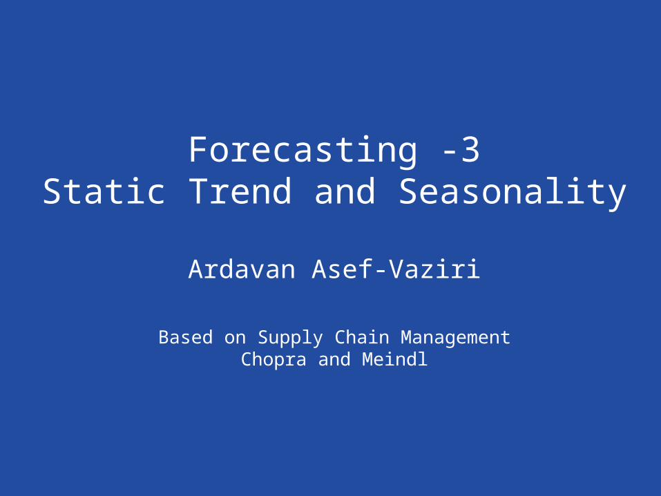
Characteristics of Forecasts
Forecasts are rarely perfect because of
randomness.
Beside the average, we also need a
measure of variations– Standard deviation.
Forecasts are more accurate for groups of
items than for individuals.
Forecast accuracy decreases as time
horizon increases.
Trend and Seasonality; Static3Ardavan Asef-Vaziri
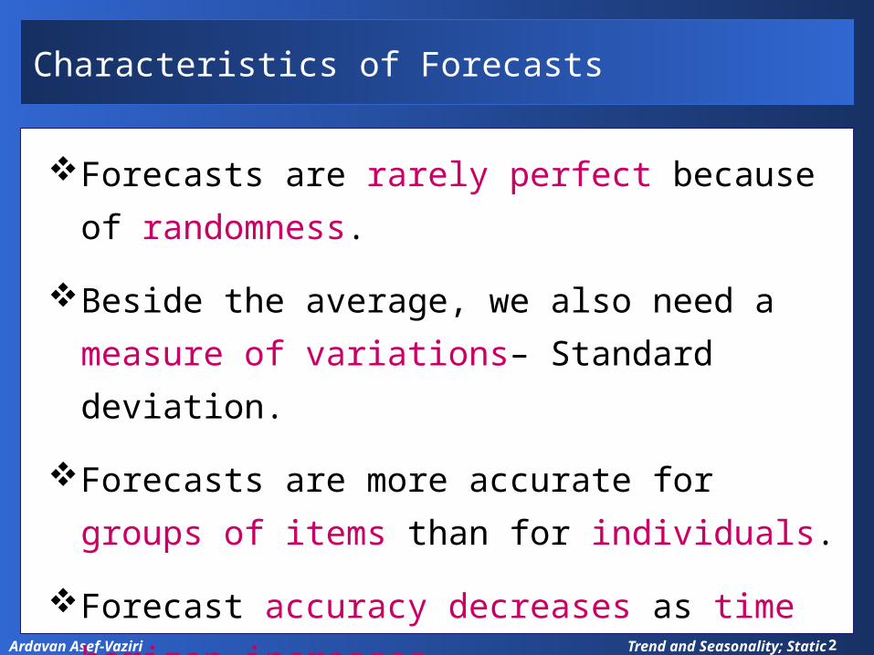
Forecasting Methods
Qualitative: primarily subjective; rely on judgment
and opinion
Time Series: use historical demand only Static
Adaptive
Causal: use the relationship between demand and
some other factor to develop forecast
Simulation Imitate consumer choices that give rise to demand
Can combine time series and causal methods
Trend and Seasonality; Static4Ardavan Asef-Vaziri
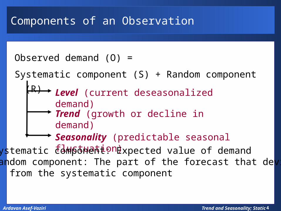
Components of an Observation
Observed demand (O) =
Systematic component (S) + Random component (R)
Level (current deseasonalized demand)
Trend (growth or decline in demand)
Seasonality (predictable seasonal fluctuation) Systematic component: Expected value of demand Random component: The part of the forecast that deviates
from the systematic component
Trend and Seasonality; Static5Ardavan Asef-Vaziri
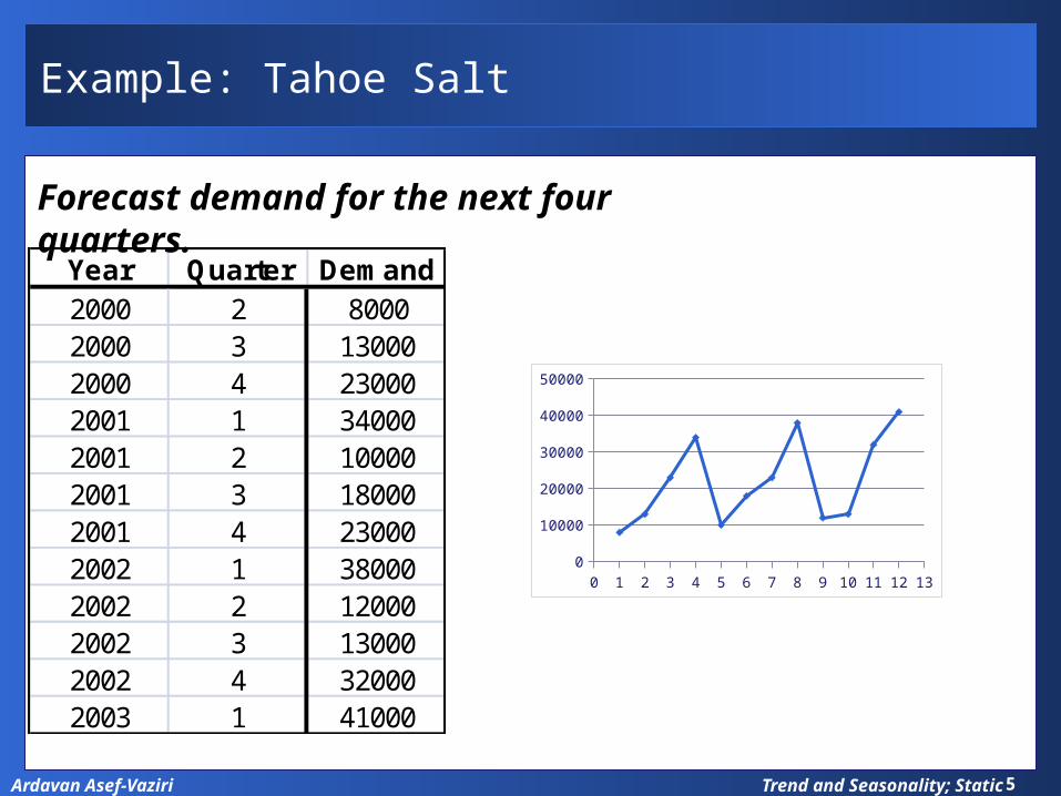
Example: Tahoe Salt
Year Quarter Demand2000 2 80002000 3 130002000 4 230002001 1 340002001 2 100002001 3 180002001 4 230002002 1 380002002 2 120002002 3 130002002 4 320002003 1 41000
Forecast demand for the next four quarters.
0 1 2 3 4 5 6 7 8 9 10 11 12 130
5000
10000
15000
20000
25000
30000
35000
40000
45000
Trend and Seasonality; Static6Ardavan Asef-Vaziri
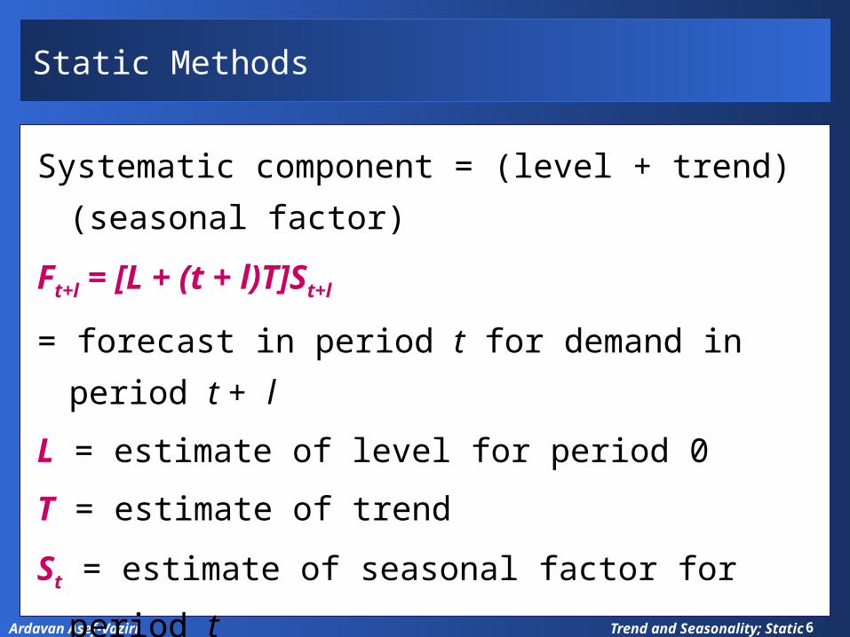
Static Methods
Systematic component = (level + trend)(seasonal factor)
Ft+l = [L + (t + l)T]St+l
= forecast in period t for demand in period t + l
L = estimate of level for period 0
T = estimate of trend
St = estimate of seasonal factor for period t
Dt = actual demand in period t
Ft = forecast of demand in period t
Trend and Seasonality; Static7Ardavan Asef-Vaziri
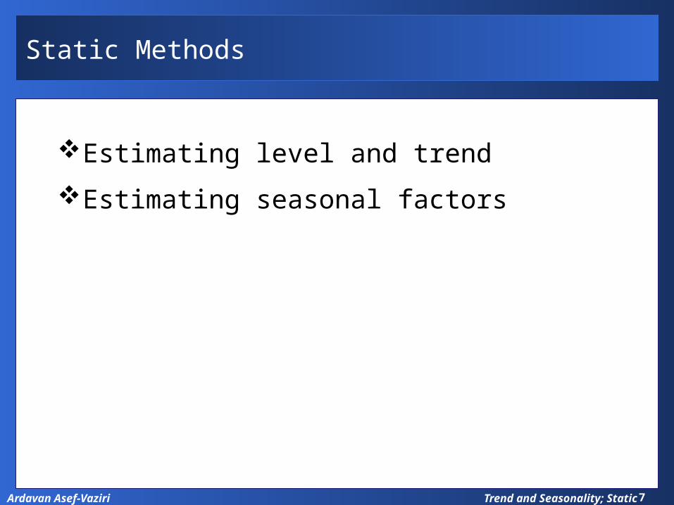
Static Methods
Estimating level and trend
Estimating seasonal factors
Trend and Seasonality; Static8Ardavan Asef-Vaziri
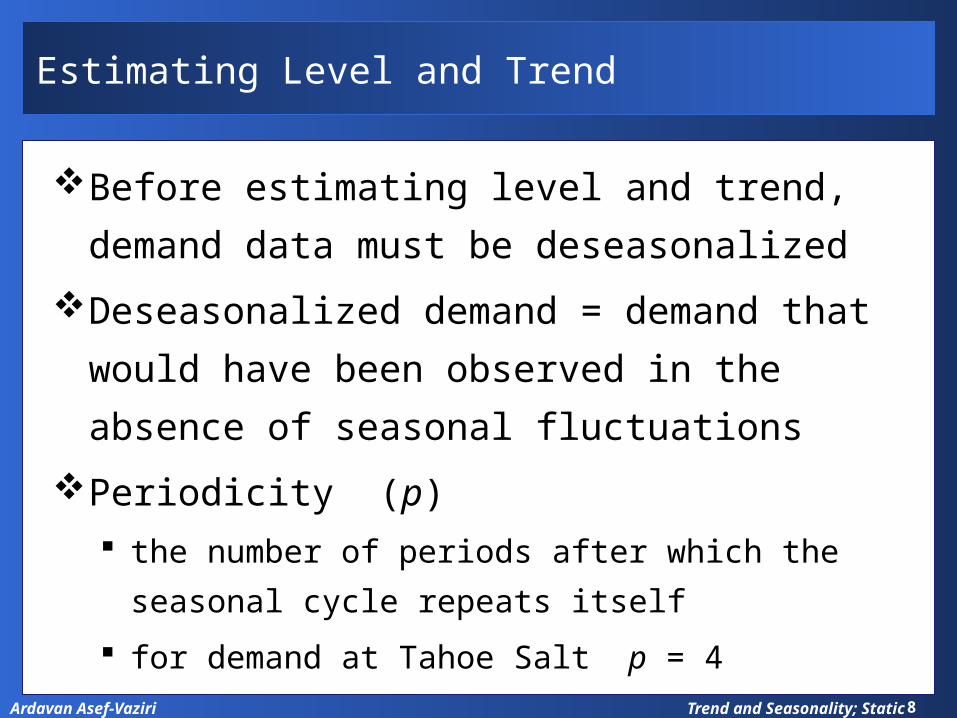
Estimating Level and Trend
Before estimating level and trend, demand
data must be deseasonalized
Deseasonalized demand = demand that
would have been observed in the absence
of seasonal fluctuations
Periodicity (p) the number of periods after which the seasonal
cycle repeats itself
for demand at Tahoe Salt p = 4
Trend and Seasonality; Static9Ardavan Asef-Vaziri
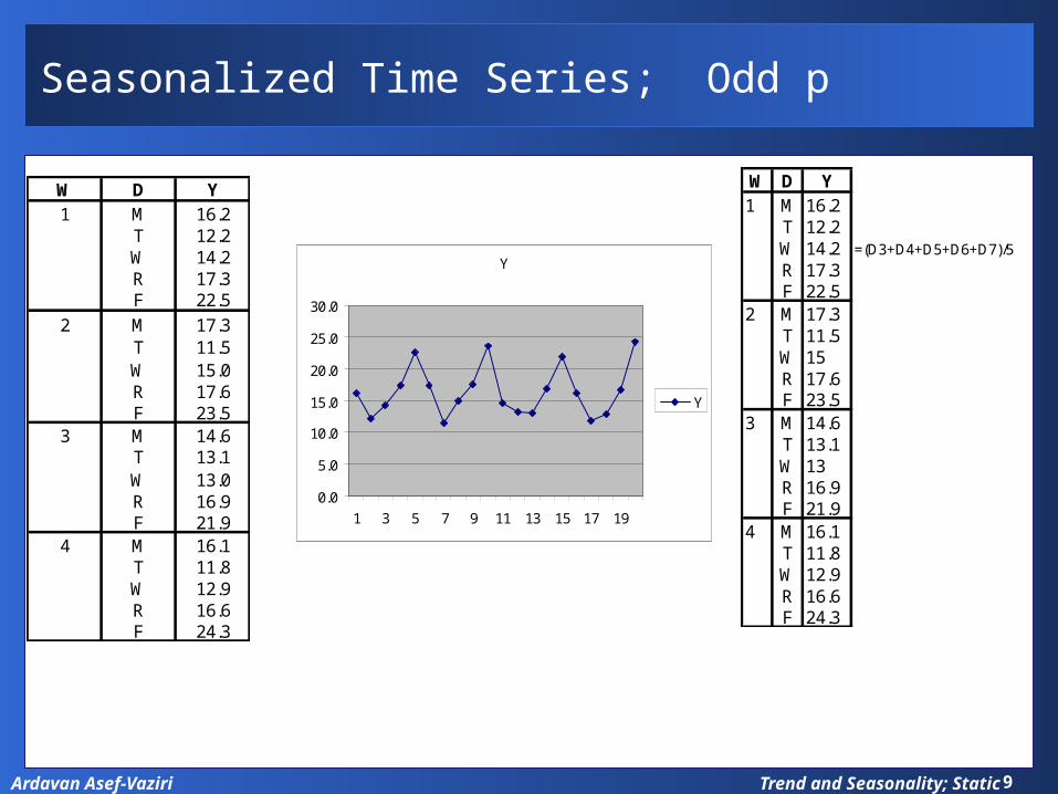
Seasonalized Time Series; Odd p
W D Y1 M 16.2
T 12.2W 14.2R 17.3F 22.5
2 M 17.3T 11.5W 15.0R 17.6F 23.5
3 M 14.6T 13.1W 13.0R 16.9F 21.9
4 M 16.1T 11.8W 12.9R 16.6F 24.3
Y
0.0
5.0
10.0
15.0
20.0
25.0
30.0
1 3 5 7 9 11 13 15 17 19
Y
W D Y1 M 16.2
T 12.2W 14.2 =(D3+D4+D5+D6+D7)/5
R 17.3F 22.5
2 M 17.3T 11.5W 15R 17.6F 23.5
3 M 14.6T 13.1W 13R 16.9F 21.9
4 M 16.1T 11.8W 12.9R 16.6F 24.3
Trend and Seasonality; Static10Ardavan Asef-Vaziri
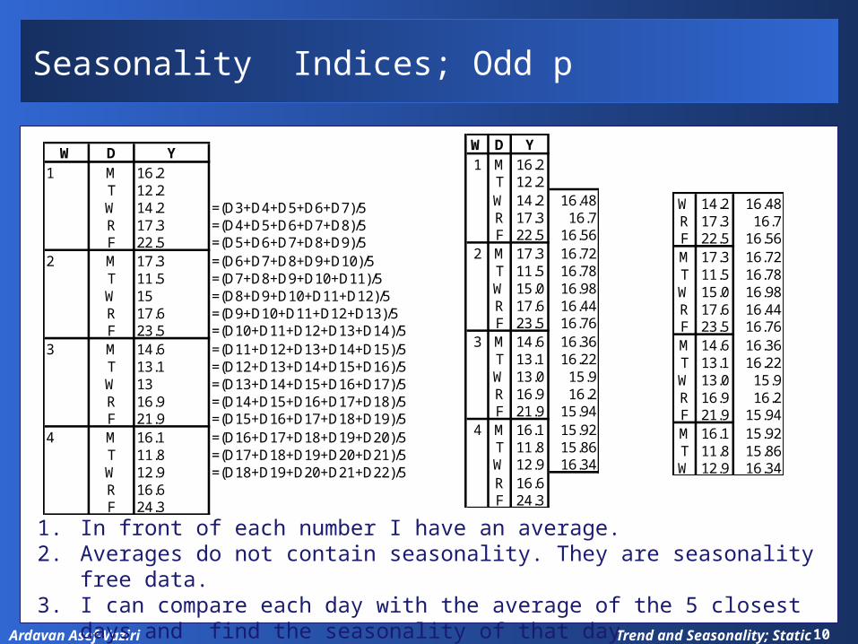
Seasonality Indices; Odd p
W D Y1 M 16.2
T 12.2W 14.2 =(D3+D4+D5+D6+D7)/5R 17.3 =(D4+D5+D6+D7+D8)/5F 22.5 =(D5+D6+D7+D8+D9)/5
2 M 17.3 =(D6+D7+D8+D9+D10)/5T 11.5 =(D7+D8+D9+D10+D11)/5W 15 =(D8+D9+D10+D11+D12)/5R 17.6 =(D9+D10+D11+D12+D13)/5F 23.5 =(D10+D11+D12+D13+D14)/5
3 M 14.6 =(D11+D12+D13+D14+D15)/5T 13.1 =(D12+D13+D14+D15+D16)/5W 13 =(D13+D14+D15+D16+D17)/5R 16.9 =(D14+D15+D16+D17+D18)/5F 21.9 =(D15+D16+D17+D18+D19)/5
4 M 16.1 =(D16+D17+D18+D19+D20)/5T 11.8 =(D17+D18+D19+D20+D21)/5W 12.9 =(D18+D19+D20+D21+D22)/5R 16.6F 24.3
W D Y1 M 16.2
T 12.2W 14.2 16.48R 17.3 16.7F 22.5 16.56
2 M 17.3 16.72T 11.5 16.78W 15.0 16.98R 17.6 16.44F 23.5 16.76
3 M 14.6 16.36T 13.1 16.22W 13.0 15.9R 16.9 16.2F 21.9 15.94
4 M 16.1 15.92T 11.8 15.86W 12.9 16.34R 16.6F 24.3
W 14.2 16.48R 17.3 16.7F 22.5 16.56M 17.3 16.72T 11.5 16.78W 15.0 16.98R 17.6 16.44F 23.5 16.76M 14.6 16.36T 13.1 16.22W 13.0 15.9R 16.9 16.2F 21.9 15.94M 16.1 15.92T 11.8 15.86W 12.9 16.34
1. In front of each number I have an average.2. Averages do not contain seasonality. They are seasonality free data. 3. I can compare each day with the average of the 5 closest days and find the
seasonality of that day
Trend and Seasonality; Static11Ardavan Asef-Vaziri
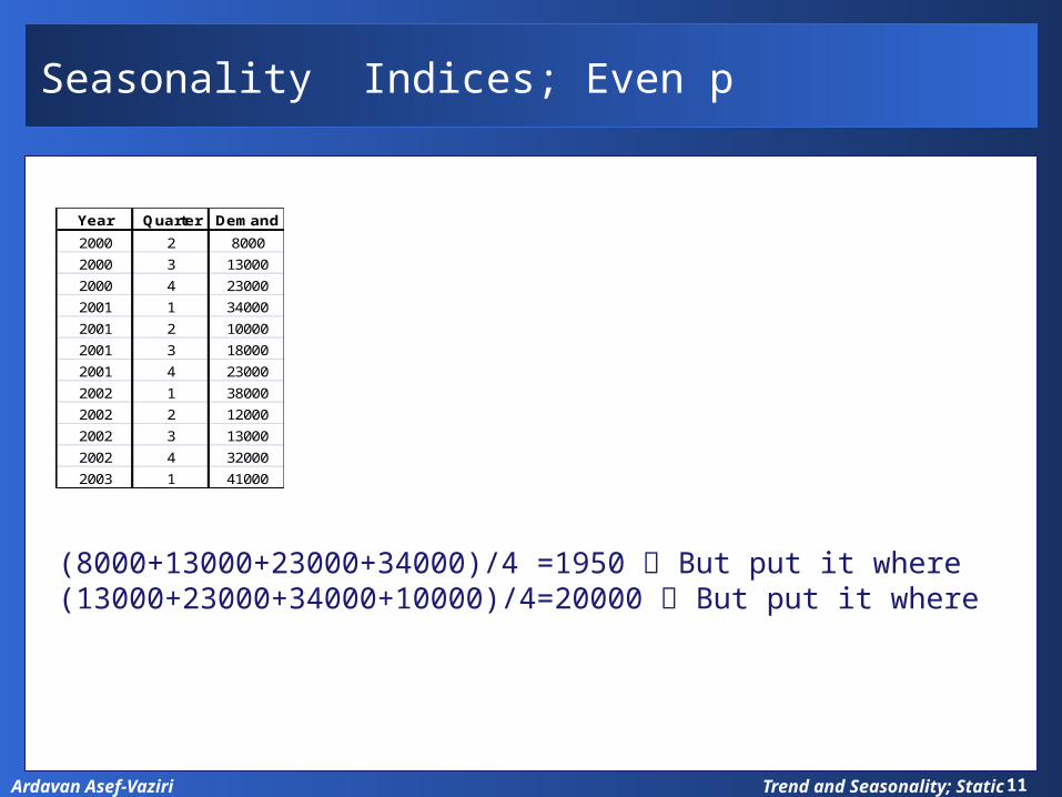
Seasonality Indices; Even p
(8000+13000+23000+34000)/4 =1950 But put it where(13000+23000+34000+10000)/4=20000 But put it where
Year Quarter Demand
2000 2 8000
2000 3 13000
2000 4 23000
2001 1 34000
2001 2 10000
2001 3 18000
2001 4 23000
2002 1 38000
2002 2 12000
2002 3 13000
2002 4 32000
2003 1 41000
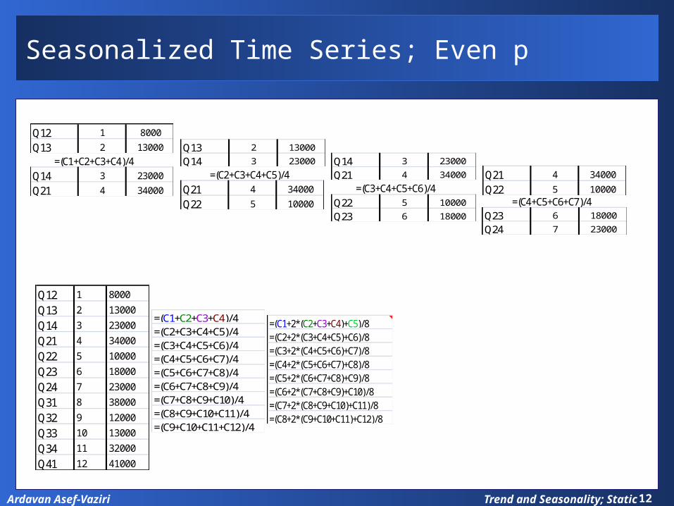
Trend and Seasonality; Static12Ardavan Asef-Vaziri
Seasonalized Time Series; Even p
Q12 1 8000
Q13 2 13000
Q14 3 23000
Q21 4 34000
Q13 2 13000
Q14 3 23000
Q21 4 34000
Q22 5 10000
Q14 3 23000
Q21 4 34000
Q22 5 10000
Q23 6 18000
Q21 4 34000
Q22 5 10000
Q23 6 18000
Q24 7 23000
=(C1+C2+C3+C4)/4=(C2+C3+C4+C5)/4
=(C3+C4+C5+C6)/4=(C4+C5+C6+C7)/4
Q12 1 8000
Q13 2 13000
Q14 3 23000
Q21 4 34000
Q22 5 10000
Q23 6 18000
Q24 7 23000
Q31 8 38000
Q32 9 12000
Q33 10 13000
Q34 11 32000
Q41 12 41000
=(C1+C2+C3+C4)/4=(C2+C3+C4+C5)/4=(C3+C4+C5+C6)/4=(C4+C5+C6+C7)/4=(C5+C6+C7+C8)/4=(C6+C7+C8+C9)/4=(C7+C8+C9+C10)/4=(C8+C9+C10+C11)/4=(C9+C10+C11+C12)/4
=(C1+2*(C2+C3+C4)+C5)/8=(C2+2*(C3+C4+C5)+C6)/8=(C3+2*(C4+C5+C6)+C7)/8=(C4+2*(C5+C6+C7)+C8)/8=(C5+2*(C6+C7+C8)+C9)/8=(C6+2*(C7+C8+C9)+C10)/8=(C7+2*(C8+C9+C10)+C11)/8=(C8+2*(C9+C10+C11)+C12)/8
Trend and Seasonality; Static13Ardavan Asef-Vaziri
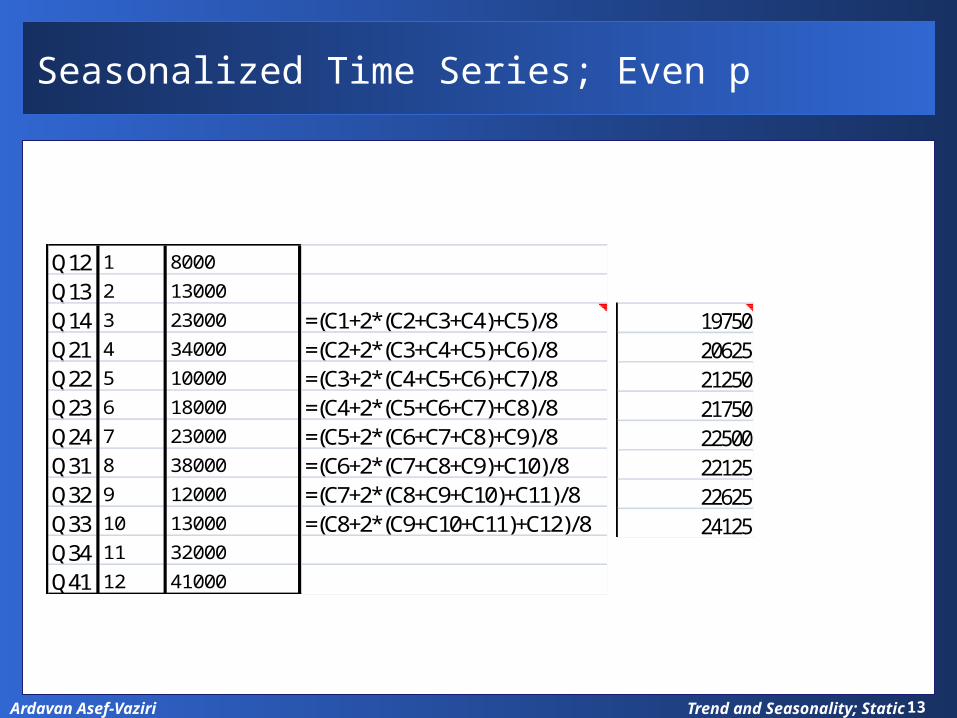
Seasonalized Time Series; Even p
Q12 1 8000
Q13 2 13000
Q14 3 23000 =(C1+2*(C2+C3+C4)+C5)/8Q21 4 34000 =(C2+2*(C3+C4+C5)+C6)/8Q22 5 10000 =(C3+2*(C4+C5+C6)+C7)/8Q23 6 18000 =(C4+2*(C5+C6+C7)+C8)/8Q24 7 23000 =(C5+2*(C6+C7+C8)+C9)/8Q31 8 38000 =(C6+2*(C7+C8+C9)+C10)/8Q32 9 12000 =(C7+2*(C8+C9+C10)+C11)/8Q33 10 13000 =(C8+2*(C9+C10+C11)+C12)/8Q34 11 32000
Q41 12 41000
1975020625212502175022500221252262524125
Trend and Seasonality; Static14Ardavan Asef-Vaziri
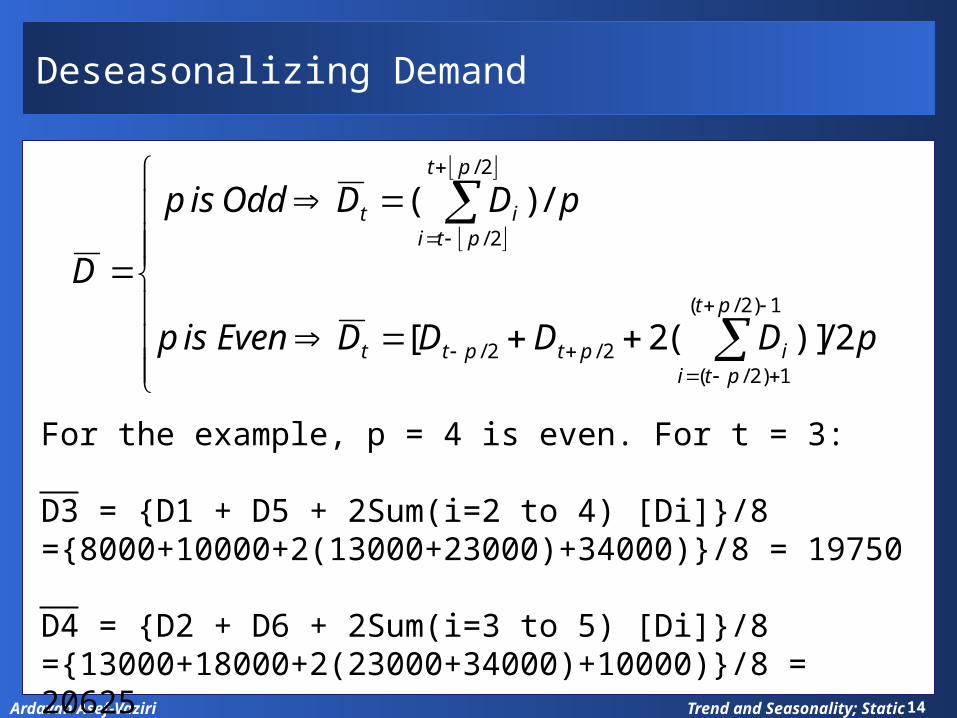
Deseasonalizing Demand
pDDDDEvenisp
pDDOddisp
Dpt
ptiiptptt
pt
ptiit
2/)](2[
/)(
1)2/(
1)2/(2/2/
2/
2/
For the example, p = 4 is even. For t = 3:
D3 = {D1 + D5 + 2Sum(i=2 to 4) [Di]}/8={8000+10000+2(13000+23000)+34000)}/8 = 19750
D4 = {D2 + D6 + 2Sum(i=3 to 5) [Di]}/8={13000+18000+2(23000+34000)+10000)}/8 = 20625
Trend and Seasonality; Static15Ardavan Asef-Vaziri
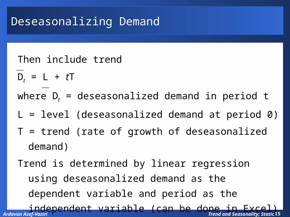
Deseasonalizing Demand
Then include trend
Dt = L + tT
where Dt = deseasonalized demand in period t
L = level (deseasonalized demand at period 0)
T = trend (rate of growth of deseasonalized demand)
Trend is determined by linear regression using deseasonalized
demand as the dependent variable and period as the independent
variable (can be done in Excel)
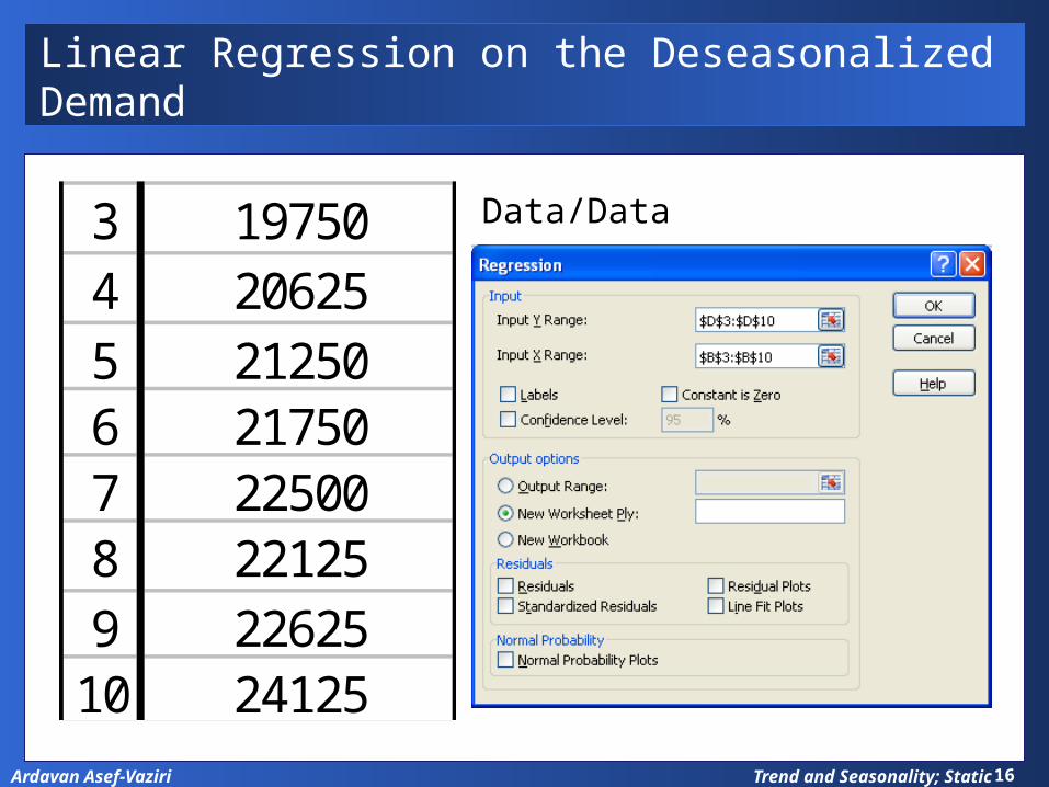
Trend and Seasonality; Static16Ardavan Asef-Vaziri
Linear Regression on the Deseasonalized Demand
3 197504 206255 212506 217507 225008 221259 22625
10 24125
Data/Data Analysis/Regression
Trend and Seasonality; Static17Ardavan Asef-Vaziri
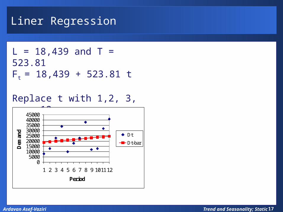
Liner Regression
L = 18,439 and T = 523.81Ft = 18,439 + 523.81 t
Replace t with 1,2, 3, ….., 12
05000
1000015000200002500030000350004000045000
1 2 3 4 5 6 7 8 9 1011 12
Demand
Period
Dt
Dt-bar
Trend and Seasonality; Static18Ardavan Asef-Vaziri
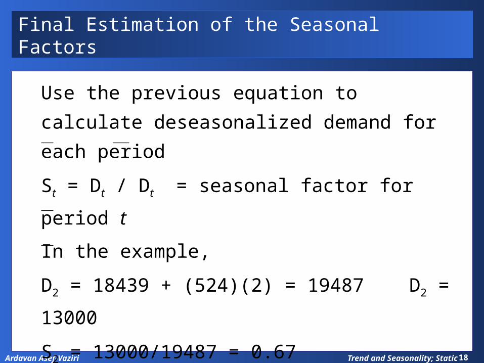
Final Estimation of the Seasonal Factors
Use the previous equation to calculate
deseasonalized demand for each period
St = Dt / Dt = seasonal factor for period t
In the example,
D2 = 18439 + (524)(2) = 19487 D2 =
13000
S2 = 13000/19487 = 0.67
The seasonal factors for the other periods
are calculated in the same manner
Trend and Seasonality; Static19Ardavan Asef-Vaziri
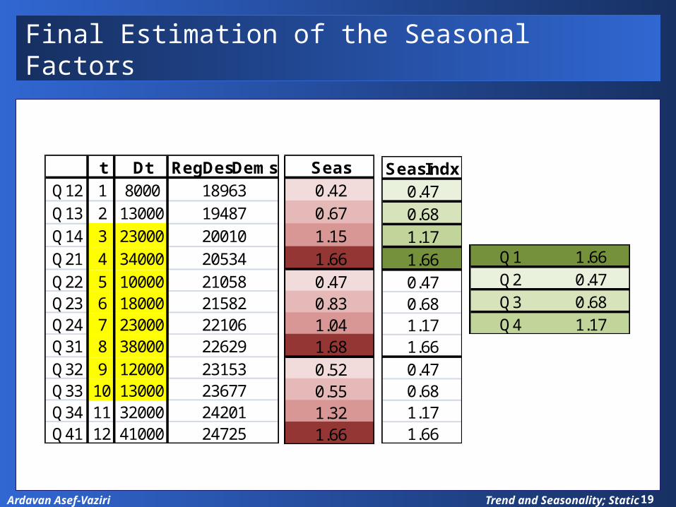
Final Estimation of the Seasonal Factors
t Dt RegDesDemsQ12 1 8000 18963Q13 2 13000 19487Q14 3 23000 20010Q21 4 34000 20534Q22 5 10000 21058Q23 6 18000 21582Q24 7 23000 22106Q31 8 38000 22629Q32 9 12000 23153Q33 10 13000 23677Q34 11 32000 24201Q41 12 41000 24725
Seas0.420.671.151.660.470.831.041.680.520.551.321.66
SeasIndx0.470.681.171.660.470.681.171.660.470.681.171.66
Q1 1.66Q2 0.47Q3 0.68Q4 1.17
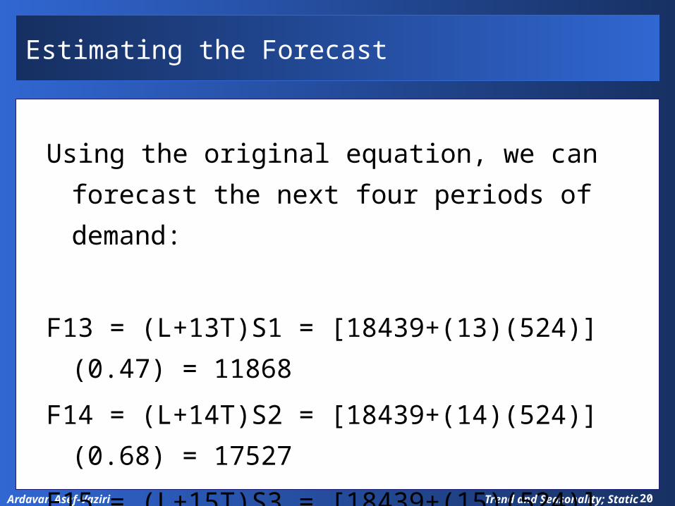
Trend and Seasonality; Static20Ardavan Asef-Vaziri
Estimating the Forecast
Using the original equation, we can forecast the next
four periods of demand:
F13 = (L+13T)S1 = [18439+(13)(524)](0.47) = 11868
F14 = (L+14T)S2 = [18439+(14)(524)](0.68) = 17527
F15 = (L+15T)S3 = [18439+(15)(524)](1.17) = 30770
F16 = (L+16T)S4 = [18439+(16)(524)](1.67) = 44794