Treatment and Reuse of Wastewater of Fish Processing Industry

Treatment and Reuse of Wastewater of Fish Processing Industry

Principal Investigator:

Final Report 2019

Dr. Zubair Ahmed, U.S.-Pakistan Center for Advanced Studies in Water, Mehran University of Engineering and Technology, Jamshoro, Pakistan

AcknowledgmentThis work was made possible by the support of the United States Government and the American people through the United States Agency for International Development (USAID).

CitationAhmed, Z. (2019). Treatment and reuse of wastewater of fish processing industry. U.S.-Pakistan Center for Advanced Studies in Water (USPCAS-W), MUET, Jamshoro, Pakistan

© All rights reserved by USPCAS-W. The author encourages fair use of this material for non-commercial purposes with proper citation.

Author

Dr. Zubair Ahmed, U.S.-Pakistan Center for Advanced Studies in Water (USPCAS-W), Mehran University of Engineering and Technology, Jamshoro, Pakistan

ISBN978-969-7970-03-2

DisclaimerThe contents of the report are the sole responsibility of the author and do not necessarily reflect the views of the funding agency and the institutions they work for.

Contributors

Principal Investigator

Dr. Zubair AhmedProfessor USPCAS-W, Mehran University of Engineering and TechnologyJamshoro, Pakistan

International Expert

Dr. Jennifer Lee WeidhaasAssociate Professor, Department of Civil and Environmental Engineering,University of Utah, Salt Lake City, USA

Team Members

� Dr. Rasool Bux Mahar, Professor, USPCAS-W, Mehran University of Engineering and Technology, Jamshoro, Pakistan

� Dr. Naveed Ahmed Qambrani, Assistant Professor, USPCAS-W, Mehran University of Engineering and Technology, Jamshoro, Pakistan

� Dr. Asmatullah, Assistant Professor, USPCAS-W, Mehran University of Engineering and Technology, Jamshoro, Pakistan

� Dr. Sara Hassan, Assistant Professor, USPCAS-W, Mehran University of Engineering and Technology, Jamshoro, Pakistan

� Mr. Barkatullah, Research Associate, USPCAS-W, Mehran University of Engineering and Technology, Jamshoro, Pakistan

� Ms. Kiran Memon, MS student, USPCAS-W, Mehran University of Engineering and Technology, Jamshoro, Pakistan

� Mr. Suresh Kumar, MS student, USPCAS-W, Mehran University of Engineering and Technology, Jamshoro, Pakistan

� Ms. Kashaf Koonj Soomro, MS student, USPCAS-W, Mehran University of Engineering and Technology, Jamshoro, Pakistan

i

TABLE OF CONTENTSACRONYMS AND ABBREVIATIONS . . . . . . . . . . . . . . . . . . . . . . . . . . . . . . . . . . . . . . . . . viiACKNOWLEDGMENTS . . . . . . . . . . . . . . . . . . . . . . . . . . . . . . . . . . . . . . . . . . . . . . . . . . . viiiEXECUTIVE SUMMARY . . . . . . . . . . . . . . . . . . . . . . . . . . . . . . . . . . . . . . . . . . . . . . . . . . . .ix1. INTRODUCTION . . . . . . . . . . . . . . . . . . . . . . . . . . . . . . . . . . . . . . . . . . . . . . . . . . . . . . . 1

1.1 Background of the Project . . . . . . . . . . . . . . . . . . . . . . . . . . . . . . . . . . . . . . . . . . . 11.2 Objectives of the Project . . . . . . . . . . . . . . . . . . . . . . . . . . . . . . . . . . . . . . . . . . . . 2

2. MATERIALS AND METHODS . . . . . . . . . . . . . . . . . . . . . . . . . . . . . . . . . . . . . . . . . . . . . 32.1 Sampling and Characterization of Water Utilized and Wastewater Generated . . . 42.2 Quantification of Water Utilized and Wastewater Generated . . . . . . . . . . . . . . . . 52.3 Estimation of Pollutant Generation from Different Streams and the

Combined Stream . . . . . . . . . . . . . . . . . . . . . . . . . . . . . . . . . . . . . . . . . . . . . . . . . 62.4 Overview of the SAAM and ECO Process . . . . . . . . . . . . . . . . . . . . . . . . . . . . . . 72.5 Setup of the Bench-scale SAAM . . . . . . . . . . . . . . . . . . . . . . . . . . . . . . . . . . . . . . 82.6 Operation of the Bench-scale SAAM. . . . . . . . . . . . . . . . . . . . . . . . . . . . . . . . . . . 92.7 Metagenomic Sequencing . . . . . . . . . . . . . . . . . . . . . . . . . . . . . . . . . . . . . . . . . . 10

2.7.1 Sample collection . . . . . . . . . . . . . . . . . . . . . . . . . . . . . . . . . . . . . . . . . . 102.7.2 Sample preparation . . . . . . . . . . . . . . . . . . . . . . . . . . . . . . . . . . . . . . . . . 102.7.3 DNA extraction . . . . . . . . . . . . . . . . . . . . . . . . . . . . . . . . . . . . . . . . . . . . . 102.7.4 Library preparation and next-generation sequencing (NGS) . . . . . . . . . . 102.7.5 Bioinformatics analysis . . . . . . . . . . . . . . . . . . . . . . . . . . . . . . . . . . . . . . 11

2.8 Fluorescence in-Situ Hybridization . . . . . . . . . . . . . . . . . . . . . . . . . . . . . . . . . . . 112.8.1 Cell fixation and storage . . . . . . . . . . . . . . . . . . . . . . . . . . . . . . . . . . . . . 112.8.2 Slide preparation . . . . . . . . . . . . . . . . . . . . . . . . . . . . . . . . . . . . . . . . . . . 112.8.3 Oligonucleotide probes . . . . . . . . . . . . . . . . . . . . . . . . . . . . . . . . . . . . . . 112.8.4 Hybridization with probes . . . . . . . . . . . . . . . . . . . . . . . . . . . . . . . . . . . . 112.8.5 Washing . . . . . . . . . . . . . . . . . . . . . . . . . . . . . . . . . . . . . . . . . . . . . . . . . . 112.8.6 DAPI counterstaining . . . . . . . . . . . . . . . . . . . . . . . . . . . . . . . . . . . . . . . . 122.8.7 Microscopy . . . . . . . . . . . . . . . . . . . . . . . . . . . . . . . . . . . . . . . . . . . . . . . 122.8.8 FISH analysis . . . . . . . . . . . . . . . . . . . . . . . . . . . . . . . . . . . . . . . . . . . . . 12

2.9 Setup of the Pilot-scale ECO unit . . . . . . . . . . . . . . . . . . . . . . . . . . . . . . . . . . . . 142.10 Operation of Pilot-scale ECO unit . . . . . . . . . . . . . . . . . . . . . . . . . . . . . . . . . . . . 172.11 Cost-benefit Analysis . . . . . . . . . . . . . . . . . . . . . . . . . . . . . . . . . . . . . . . . . . . . . . 182.12 Environmental Impacts using Life Cycle Assessment . . . . . . . . . . . . . . . . . . . . . 19

2.12.1 Goal and scope of the impact assessment through LCA. . . . . . . . . . . . . 202.12.2 Life cycle inventory . . . . . . . . . . . . . . . . . . . . . . . . . . . . . . . . . . . . . . . . . 202.12.3 Life cycle impact assessment . . . . . . . . . . . . . . . . . . . . . . . . . . . . . . . . . 21

2.13 Best Management Practices . . . . . . . . . . . . . . . . . . . . . . . . . . . . . . . . . . . . . . . . 22

ii

2.13.1 Pollution reduction by screening . . . . . . . . . . . . . . . . . . . . . . . . . . . . . . . 222.13.2 Segregation of drainage points . . . . . . . . . . . . . . . . . . . . . . . . . . . . . . . . 232.13.3 Schedule/work plan of the project . . . . . . . . . . . . . . . . . . . . . . . . . . . . . . 23

3. RESULTS AND DISCUSSION. . . . . . . . . . . . . . . . . . . . . . . . . . . . . . . . . . . . . . . . . . . . 253.1 Quantification of Freshwater Utilization . . . . . . . . . . . . . . . . . . . . . . . . . . . . . . . . 253.2 Characterization of Freshwater Consumed . . . . . . . . . . . . . . . . . . . . . . . . . . . . . 253.3 Characterization of the Wastewater from the Facility . . . . . . . . . . . . . . . . . . . . . 263.4 Estimated Characteristics of the Different Streams and Combined Stream . . . . 293.5 Treatment of Shrimp Processing Effluent using SAAM . . . . . . . . . . . . . . . . . . . . 313.6 MLSS and MLVSS Concentration in Anoxic/Anaerobic and Aerobic Reactor . . . 333.7 TDS Concentration in Influent and Effluent of SAAM . . . . . . . . . . . . . . . . . . . . . 343.8 Removal of COD in SAAM . . . . . . . . . . . . . . . . . . . . . . . . . . . . . . . . . . . . . . . . . 353.9 Removal of TN and TP in SAAM . . . . . . . . . . . . . . . . . . . . . . . . . . . . . . . . . . . . . 363.10 Fluorescence in-situ Hybridization . . . . . . . . . . . . . . . . . . . . . . . . . . . . . . . . . . . 373.11 16s rRNA Metagenomic Sequencing . . . . . . . . . . . . . . . . . . . . . . . . . . . . . . . . . 42

3.11.1 Phylum-level . . . . . . . . . . . . . . . . . . . . . . . . . . . . . . . . . . . . . . . . . . . . . . 433.11.2 Class-level . . . . . . . . . . . . . . . . . . . . . . . . . . . . . . . . . . . . . . . . . . . . . . . 433.11.3 Order-level . . . . . . . . . . . . . . . . . . . . . . . . . . . . . . . . . . . . . . . . . . . . . . . 433.11.4 Family-level . . . . . . . . . . . . . . . . . . . . . . . . . . . . . . . . . . . . . . . . . . . . . . . 443.11.5 Genus-level . . . . . . . . . . . . . . . . . . . . . . . . . . . . . . . . . . . . . . . . . . . . . . 453.11.6 Species-level analysis . . . . . . . . . . . . . . . . . . . . . . . . . . . . . . . . . . . . . . . 46

3.12 Biological Testing of Treated Effluent . . . . . . . . . . . . . . . . . . . . . . . . . . . . . . . . . 463.13 Treatment of Shrimp Processing Effluent using ECO System . . . . . . . . . . . . . . 46

3.13.1 Removal of COD in the ECO process . . . . . . . . . . . . . . . . . . . . . . . . . . . 473.13.2 Removal of turbidity in the ECO process . . . . . . . . . . . . . . . . . . . . . . . . . 503.13.3 Removal of color in the ECO process . . . . . . . . . . . . . . . . . . . . . . . . . . . 50

3.14 Comparison of the Two Treatment Systems . . . . . . . . . . . . . . . . . . . . . . . . . . . . 503.15 Comparison of Benefits of Membrane Bioreactor versus Reverse

Osmosis System . . . . . . . . . . . . . . . . . . . . . . . . . . . . . . . . . . . . . . . . . . . . . . . . . 513.16 Environmental Impacts of Shrimps Processing . . . . . . . . . . . . . . . . . . . . . . . . . . 52

3.16.1 Environmental impacts . . . . . . . . . . . . . . . . . . . . . . . . . . . . . . . . . . . . . . 523.16.2 Targeted impact categories comparison . . . . . . . . . . . . . . . . . . . . . . . . . 53

3.17 Water Reuse within the Shrimp Processing Facility . . . . . . . . . . . . . . . . . . . . . . 553.17.1 Pollution reduction after sieving . . . . . . . . . . . . . . . . . . . . . . . . . . . . . . . . 553.17.2 Segregation of drainage points at the facility. . . . . . . . . . . . . . . . . . . . . . 553.17.3 Reuse possibility in the process and floor washing . . . . . . . . . . . . . . . . . 55

3.18 Strategy for Burden-sharing with Other Polluting Industrial Sectors within the Area and Funds Arrangement for Environmental Initiatives . . . . . . . . 573.18.1 Need for estimation environmental damage costs . . . . . . . . . . . . . . . . . 58

iii

3.18.2 Implementation of an environmental levy system . . . . . . . . . . . . . . . . . . 583.18.3 Funds arrangements for environmental initiatives . . . . . . . . . . . . . . . . . . 59

3.19 Research Output . . . . . . . . . . . . . . . . . . . . . . . . . . . . . . . . . . . . . . . . . . . . . . . . . 603.19.1 Research Papers Presented in Conferences . . . . . . . . . . . . . . . . . . . . . 603.19.2 Posters Presentations . . . . . . . . . . . . . . . . . . . . . . . . . . . . . . . . . . . . . . 603.19.3 Research Papers . . . . . . . . . . . . . . . . . . . . . . . . . . . . . . . . . . . . . . . . . . . 603.19.4 M.Sc. Thesis . . . . . . . . . . . . . . . . . . . . . . . . . . . . . . . . . . . . . . . . . . . . . . 613.19.5 Project Results Dissemination Seminars . . . . . . . . . . . . . . . . . . . . . . . . . 61

4 CONCLUSION AND RECOMMENDATIONS . . . . . . . . . . . . . . . . . . . . . . . . . . . . . . . . 624.1 Conclusion. . . . . . . . . . . . . . . . . . . . . . . . . . . . . . . . . . . . . . . . . . . . . . . . . . . . . . 624.2 Recommendations . . . . . . . . . . . . . . . . . . . . . . . . . . . . . . . . . . . . . . . . . . . . . . . 62REFERENCES . . . . . . . . . . . . . . . . . . . . . . . . . . . . . . . . . . . . . . . . . . . . . . . . . . . . . . . 63Annex-1: Combined characteristics of shrimp processing wastewater . . . . . . . . . . . . . 66Annex-2: NEQS guideline values . . . . . . . . . . . . . . . . . . . . . . . . . . . . . . . . . . . . . . . . . 67Annex-3: Saminar invitation cards . . . . . . . . . . . . . . . . . . . . . . . . . . . . . . . . . . . . . . . . . 68Annex-4: Project Results Dissemination Seminars at Karachi . . . . . . . . . . . . . . . . . . . 69Annex-5: Project Results Dissemination Seminars at USPCAS-W, MUET, Jamshoro . 70

iv

LIST OF TABLESTable 2.1: Seasons of production, duration of seasons, and production capacities of

the fish processing facility . . . . . . . . . . . . . . . . . . . . . . . . . . . . . . . . . . . . . . . . . . . 5

Table 2.2: Wastewater generation from individual processes based on production seasons 5

Table 2.3: Flow rates of pumps installed at the facility . . . . . . . . . . . . . . . . . . . . . . . . . . . . . . 6

Table 2.4: Operational parameters of the SAAM . . . . . . . . . . . . . . . . . . . . . . . . . . . . . . . . . . 9

Table 2.5: Sequence of oligonucleotide probes used in this study . . . . . . . . . . . . . . . . . . . . 13

Table 2.6: Specification and dimensions of the sand filter and cartridge filter used

prior to the ECO system. . . . . . . . . . . . . . . . . . . . . . . . . . . . . . . . . . . . . . . . . . . . 16

Table 2.7: Details of the units added after the ECO unit in Phase-II. . . . . . . . . . . . . . . . . . . 17

Table 2.8: Operating parameters of the ECO unit at the pilot-scale. . . . . . . . . . . . . . . . . . . 18

Table 2.9: Inventory data of the shrimps processing per kg of raw shrimps processed. . . . 21

Table 2.10: Schedule/work plan of the project . . . . . . . . . . . . . . . . . . . . . . . . . . . . . . . . . . . . 24

Table 3.1: Characteristics of freshwater used in the shrimp processing facility . . . . . . . . . . 26

Table 3.2: Calculation of pollutant discharge per liter of shrimps processing wastewater . . 30

Table 3.3: Pollutant discharge per kg of shrimp production . . . . . . . . . . . . . . . . . . . . . . . . . 30

Table 3.4: Phases of bench-scale SAAM operated in laboratory . . . . . . . . . . . . . . . . . . . . . 32

Table 3.5: Treatment of the shrimp processing effluent before and after SAAM treatment . 33

Table 3.6: Results from fluorescence in-situ hybridization demonstrated in the initial

and final stage on MBR . . . . . . . . . . . . . . . . . . . . . . . . . . . . . . . . . . . . . . . . . . . . 38

Table 3.7: Characteristics of the shrimp processing wastewater before and after

electrocoagulation process in Phase I . . . . . . . . . . . . . . . . . . . . . . . . . . . . . . . . . 48

Table 3.8: Characteristics of the shrimp processing wastewater before and after

electrocoagulation along with UV/H2O2 process in Phase-II . . . . . . . . . . . . . . . . 49

Table 3.9: Comparison of the treatment efficiencies of the SAAM and ECO system . . . . . . 51

Table 3.10: LCA results presented per unit of the functional unit (1 ton of raw shrimps) . . . . 52

Table 3.11: Pollution reduction after sieving of washing and soaking processes . . . . . . . . . . 55

Table 3.12: Water reuse possibility in the shrimp processing and floor cleaning . . . . . . . . . . 56

v

LIST OF FIGURESFig. 1.1: Shrimps processing steps . . . . . . . . . . . . . . . . . . . . . . . . . . . . . . . . . . . . . . . . . . . 1

Fig. 2.1: Conceptual flowchart for the possible impacts of various project activities

on the industry, ocean habitat, and economic growth . . . . . . . . . . . . . . . . . . . . . . 3

Fig. 2.2: Sampling points at the shirimp processing facility . . . . . . . . . . . . . . . . . . . . . . . . . 4

Fig. 2.3: Schematic diagram of the bench-scale SAAM. . . . . . . . . . . . . . . . . . . . . . . . . . . . 8

Fig. 2.4: Bench-scale SAAM operated at the USPCAS-W laboratory . . . . . . . . . . . . . . . . . 9

Fig. 2.5: Schematic diagram representing FISH-technique steps . . . . . . . . . . . . . . . . . . . 12

Fig. 2.6: Schematic diagram of electrocoagulation/oxidation (ECO) unit. . . . . . . . . . . . . . 14

Fig. 2.7: Schematic diagram of Phase I pilot-scale ECO unit . . . . . . . . . . . . . . . . . . . . . . 14

Fig. 2.8: Schematic diagram of the phase II pilot-scale ECO unit along with UV/

H2O2 used in Phase-II. . . . . . . . . . . . . . . . . . . . . . . . . . . . . . . . . . . . . . . . . . . . . . 15

Fig. 2.9: Schematic diagram of sand filter . . . . . . . . . . . . . . . . . . . . . . . . . . . . . . . . . . . . . 15

Fig. 2.10: ECO unit installed at the facility for the treatment of shrimp processing

wastewater . . . . . . . . . . . . . . . . . . . . . . . . . . . . . . . . . . . . . . . . . . . . . . . . . . . . . . 19

Fig. 2.11: Scenarios for wastewater treatment and environmental damages . . . . . . . . . . . 22

Fig. 2.12: Washing and soaking processes’ effluents screening . . . . . . . . . . . . . . . . . . . . . 23

Fig. 3.1: Water utilization in shrimps processing . . . . . . . . . . . . . . . . . . . . . . . . . . . . . . . . 25

Fig. 3.2: TSS and VSS concentration in different streams . . . . . . . . . . . . . . . . . . . . . . . . . 26

Fig. 3.3: TDS of shrimp processing wastewater . . . . . . . . . . . . . . . . . . . . . . . . . . . . . . . . 27

Fig. 3.4: BOD of shrimps processing wastewater . . . . . . . . . . . . . . . . . . . . . . . . . . . . . . . 27

Fig. 3.5: COD of shrimps processing wastewater . . . . . . . . . . . . . . . . . . . . . . . . . . . . . . . 28

Fig. 3.6: TN of shrimps processing wastewater . . . . . . . . . . . . . . . . . . . . . . . . . . . . . . . . . 29

Fig. 3.7: TP of shrimps processing wastewater . . . . . . . . . . . . . . . . . . . . . . . . . . . . . . . . . 29

Fig. 3.8: MLSS and MLVSS concentration in the aerobic reactor . . . . . . . . . . . . . . . . . . . 33

Fig. 3.9: MLSS and MLVSS concentration in the anoxic/anaerobic reactor . . . . . . . . . . . 34

Fig. 3.10: TDS concentration in influent and effluent of SAAM . . . . . . . . . . . . . . . . . . . . . . 35

Fig. 3.11: COD concentration in influent and effluent of SAAM . . . . . . . . . . . . . . . . . . . . . . 36

Fig. 3.12: TN concentration in the influent and effluent of the SAAM . . . . . . . . . . . . . . . . . 37

Fig. 3.13: TP concentration in the influent and effluent of the SAAM . . . . . . . . . . . . . . . . . 37

Fig. 3.14: DAPI stained cells in the sludge samples from the membrane bioreactor. . . . . . 39

Fig. 3.15: Graphical representation of microbial community dynamics showing

distribution and changes in the population, hybridized with oligonucleotide

probes . . . . . . . . . . . . . . . . . . . . . . . . . . . . . . . . . . . . . . . . . . . . . . . . . . . . . . . . . 39

Fig. 3.16: Relative abundance of β-Proteobacteria . . . . . . . . . . . . . . . . . . . . . . . . . . . . . . . 40

vi

Fig. 3.17: Relative abundance of α-Proteobacteria . . . . . . . . . . . . . . . . . . . . . . . . . . . . . . . 40

Fig. 3.18: Relative abundance of γ-Proteobacteria . . . . . . . . . . . . . . . . . . . . . . . . . . . . . . . 41

Fig. 3.19: Relative abundance of δ-Proteobacteria . . . . . . . . . . . . . . . . . . . . . . . . . . . . . . . 41

Fig. 3.20: Relative abundance of Actinobacteria . . . . . . . . . . . . . . . . . . . . . . . . . . . . . . . . . 42

Fig. 3.21: Relative abundance of Cytophaga-Flavobacteria cluster . . . . . . . . . . . . . . . . . . 42

Fig. 3.22: Phylum level of bacteria in the initial and final stage of SAAM . . . . . . . . . . . . . . 43

Fig. 3.23: Class level of bacteria in the initial and final stage of SAAM . . . . . . . . . . . . . . . . 44

Fig. 3.24: Order level of bacteria in the initial and final stage of SAAM . . . . . . . . . . . . . . . . 44

Fig. 3.25: Family level of bacteria in initial and final stage of SAAM . . . . . . . . . . . . . . . . . . 45

Fig. 3.26: Genus level of bacteria in the initial and final stage of SAAM . . . . . . . . . . . . . . . 45

Fig. 3.27: Average COD in influent, the effluent of the sand filter, and effluent from

the ECO unit . . . . . . . . . . . . . . . . . . . . . . . . . . . . . . . . . . . . . . . . . . . . . . . . . . . . 47

Fig. 3.28: Average turbidity in influent and effluent of the sand filter and effluent of

the ECO unit . . . . . . . . . . . . . . . . . . . . . . . . . . . . . . . . . . . . . . . . . . . . . . . . . . . . 50

Fig. 3.29: Average color in influent/effluent of the sand filter and effluent of the EC unit . . 51

Fig. 3.30: Relative impacts of Scenario 1 and Scenario 2 . . . . . . . . . . . . . . . . . . . . . . . . . . 52

Fig. 3.31: Marine eutrophication potential comparison . . . . . . . . . . . . . . . . . . . . . . . . . . . . 54

Fig. 3.32: Water depletion comparison . . . . . . . . . . . . . . . . . . . . . . . . . . . . . . . . . . . . . . . . 54

Fig. 3.33: Freshwater eutrophication potential comparison . . . . . . . . . . . . . . . . . . . . . . . . . 54

Fig. 3.34: Layout of the shrimp processing facility . . . . . . . . . . . . . . . . . . . . . . . . . . . . . . . . 56

vii

ACRONYMS AND ABBREVIATIONSBOD Biochemical oxygen demand

BODf Biochemical oxygen demand filtered

COD Chemical oxygen demand

CODf Chemical oxygen demand filtered

DO Dissolved oxygen

DOC Dissolved organic carbon

ECO Electrocoagulation/Oxidation

GW Ground water

H2O2 Hydrogen peroxide

HRT Hydraulic retention

LCIA Life cycle impact assessment

MUET Mehran University of Engineering and Technology

NO3--N Nitrate nitrogen

OLR Organic loading rate

(PO4)3--P Phosphate phosphorus

Qe Effluent flow rate

Qi Influent flow rate

Qr Returned sludge flow rate

SAAM Sequential anaerobic/anoxic and aerobic membrane bioreactor

SO42- Sulphate

SP Shrimp processing wastewater

SRT Sludge retention time

TDS Total dissolved solids

TN Total nitrogen

TP Total phosphorus

TSS Total suspended solids

USPCAS-W United States-Pakistan Center for Advanced Studies in Water

UV Ultraviolet

VSS Volatile suspended solids

viii

ACKNOWLEDGMENTSWe humbly express our gratitude to the Almighty Allah, Who allowed us to carry out this research project and enabled us to complete this report successfully.

The project team would like to thank all the contributors to this research report. We are thankful to Mr. Muslim S. Mohammedi, CEO M.A. Mohamedi & Co. and Vice President of Federation of Chamber of Commerce and Industry (FPCCI), for his kind support for the utilization of facilities at his shrimp processing industry.

We extend our sincere gratitude is to Dr. Bakhshal Lashari, Project Director, USPCAS-W, and Dr. Rasool Bux Mahar, Deputy Project Director (Research and Academic), for their kind guidance. The administration team of USPCAS-W has always extended helping hands to us whenever required. We are thankful to all of them, particularly to Mr. Syed Mansoor Ali Shah, Manager Finance and Grants, Dr. Kazi Suleman Memon, Manager Research, Mr. Muzafar Ali Joyo, Graphic Designer/Data Entry Operator, and Mr. Faizan, Logistic Officer. We also received valuable input from Dr. Naveed Ahmed Qambrani, Mr. Junaid Ahmed Kori, and Mr. Asif Jokhio throughout the project.

This research work was not possible without the funding from USAID and technical assistance from the University of Utah, USA. The project team is sincerely thankful to Dr. Aslam Chaudhry, Party Chief, University of Utah, and Prof. Dr. Steven Burian, Project Director of CAS-W at the University of Utah.

ix

EXECUTIVE SUMMARYThe fishing industry in Pakistan plays a vital role in the country’s economy. Karachi Fish Harbor handles about 90% of fish and seafood in Pakistan, which makes up to 95% of the seafood exports from Pakistan. With hundreds of varieties of fish species and more than 30 species of shrimps, the fishing industry brings home a considerable amount of foreign exchange, and it is also a source of employment for the labor force in the country. However, these economic benefits do not come for free. These benefits come at the cost of the environmental pollution caused by the industry. During the cleaning and washing of fish and shrimp in the processing industry, scarce freshwater is being used, whereas the wastewater generated in this process contains high organic and nutrient contents, i.e., chemical oxygen demand (COD), total nitrogen (TN) and total phosphorus (TP). In Karachi, this wastewater is discharged into the Arabian Sea without any prior treatment. Such disposal of the untreated wastewater is not only dangerous for the marine life, but it is also detrimental to the long-term economic benefits of the fish processing industry whose revenue is directly dependent upon the seafood catch. Therefore, it has become highly crucial for the seafood processing industry to take immediate actions to minimize, treat, and reuse wastewater being generated. Realizing the needs of the seafood processing industry, the US-Pakistan Center for Advanced Studies (USPCAS-W), Mehran University of Engineering and Technology (MUET), Jamshoro initiated a joint research project in collaboration with a progressive shrimp processing industry located at Karachi to determine the most efficient, feasible and economically viable treatment methodology for the wastewater of the shrimps processing industry. USAID arranged the funding of this project through USPCAS-W under the faculty seed grant program.

This study aimed to compare the environmental damages caused by the current processing system and those with the addition of wastewater treatment and water reuse systems in the existing processing system. The specific objectives of the study were: (a) characterization of the water and wastewater quality of a selected fish processing industry; (b) selection of suitable treatment process and cost comparison of selected treatment train with desalination process of the same capacity; and (c) evaluation of the pollution load reduction into the Arabian Sea upon implementation of selected treatment within the fish processing industries and development of a strategy of burden-sharing with other polluting industrial sectors within the area. The project was executed in three phases. In Phase-1, a detailed examination of fish processing steps was conducted on-site at the facility, and a wastewater recycle/reuse opportunity was explored. A sampling plan was developed considering wastewater discharge from different processing steps. Samples were taken to cover all the processing activities,

x

and overall pollution loads were calculated. The quality and quantity of freshwater consumption and wastewater generation were estimated. In Phase 2, a bench-scale sequencing anoxic/anaerobic-aerobic membrane bioreactor (SAAM) was operated at the laboratory of USPCAS-W, and a pilot-scale electrocoagulation/oxidation (ECO) unit was set up and operated in a shrimp processing facility at the Karachi Fish Harbor by introducing wastewater from the shrimp processing facility. The SAAM and ECO were operated under varying operating parameters to evaluate the performance of the treatment systems. The average COD removal achieved with the use of SAAM was 94.3%, whereas the average COD removal value was found to be 55% in the case of ECO system. Moreover, the TN, TP, DOC (dissolved organic carbon), nitrate-nitrogen (NO3

—N), and phosphate phosphorus (PO4)3--P removal of SAAM were

found to be 69.5, 53.3, 96.8, 61.7, and 94.3%, respectively. The pollutant removal efficiency of ECO unit was: 30% of TN, 76% of TP, 42% of DOC, 63% of NO3

--N, and 81% of (PO4)

3--P. The results demonstrated that the SAAM was more efficient in reducing the COD, TN, DOC and (PO4)

3--P, while the ECO system was more efficient in removing NO3

--N and TP. Overall, the SAAM was found to be more effective for shrimp wastewater treatment. In the Phase 3, an environmental study was conducted to quantify the environmental impacts caused by the shrimp processing through a life cycle assessment of a selected shrimps processing facility. The results showed the greatest reduction in impacts on freshwater eutrophication, followed by marine eutrophication and water resource depletion.

The introduction of wastewater treatment and water reuse practices, suggested in the current production system will minimize the water-oriented environmental impacts of the product that will lead the industry towards environmentally sustainable products. Moreover, the recommended in-house management practices within the industry also result in the reduction of pollution loads. Currently, fishing activities are being hampered due to environmental degradation of the coast of Karachi, which is caused by the improper discharge of wastewater from industrial/domestic sources other than the seafood processing. It is necessary to evaluate environmental damage costs from the polluters from all sources and devise a plan for imposing levy/compensation systems to the polluters/effected stakeholders.

1

1. INTRODUCTION1.1 Background of the Project

The fishing industry in Pakistan plays a vital role in the country’s economy. Pakistan has a coastline of 1,120 km, which borders the northeast of the Arabian Sea and covers the coasts of Sindh and Baluchistan with a total fishing area of approximately 300,270 km2. Karachi fish harbor handles about 90% of fish and seafood in Pakistan, which makes up to 95% of the seafood exports from Pakistan. With hundreds of varieties of fish species (including more than 30 species of shrimps) the fishing industry brings home a considerable amount of foreign exchange and it is also a source of employment for the labor force in the country. However, these economic benefits come at the cost of the environmental pollution caused by the industry. Freshwater is used for cleaning and washing of the seafood in the fish/shrimp processing industry. The steps in fish and shrimp processing are shown in Fig. 1.1.

Fig. 1.1: Shrimps processing steps

The wastewater generated in this process is high in organic and nutrient content, i.e., chemical oxygen demand (COD), total nitrogen (TN) and total phosphorus (TP), with biochemical oxygen demand (BOD) usually in the range of 1 – 72.5 kg per ton of the product (Marshall et al., 1996). This wastewater is usually discharged into the Arabian Sea without any prior treatment. It is not only dangerous for marine life, but

2

is also detrimental to the long-term economic benefits of the fish/shrimp processing industry whose revenue is directly dependent upon the seafood catch. This situation requires an urgent need to treat the wastewater, which can be reused within the industry to save water-related costs and to prevent further environmental damage. The current study is aimed to determine the most efficient, feasible, and economically viable treatment methodology for the wastewater of the shrimps processing industry, to assess environmental impacts due to wastewater being discharged, and reduction of adverse environmental impacts upon reuse of the treated wastewater within the industry.

1.2 Objectives of the Project

The specific objectives of the study were:

1. Characterization of the water and wastewater quality of a selected fish/shrimp processing industry

2. Selection of suitable treatment process and cost comparison of selected treatment train with desalination process of the same capacity

3. Evaluation of the pollution load reduction into the Arabian Sea upon implementation of selected treatment within the fish processing industries and development of a strategy of burden-sharing with other polluting industrial sectors within the area.

3

2. MATERIALS AND METHODSA conceptual framework of the research study was developed as represented by a conceptual flow chart for the possible impacts of various project activities on the industry, ocean habitat, and economic growth (Fig. 2.1).

Fig. 2.1: Conceptual flowchart for the possible impacts of various project activities on the industry, ocean habitat, and economic growth

In keeping with the conceptual framework and the objectives of this study, the overall approach is described below:

The samples of the freshwater used and the wastewater generated were collected from the facility and were characterized in the laboratory at USPCASW. A pilot-scale ECO unit and a bench-scale SAAM were set up and operated at the shrimp processing facility and US-Pakistan Center for Advanced Studies in Water (USPCAS-W), Mehran University of Engineering and Technology (MUET), Jamshoro, respectively. Both of the treatment trains were compared. Finally, a life cycle impact assessment was set up and run under two scenarios; current scenario wherein untreated wastewater is discharged into the sea and the proposed scenario in which the wastewater would be treated and reused within the industry. The results of this study will help in a better understanding of environmental pollution caused by improper wastewater disposal and reducing the pollution load into the Arabian Sea. It will also assist us in developing a strategy for the burden-sharing with other facilities of the industry in the area.

The study was conducted in three phases. The description of each phase and the activities carried out in each phase are presented below.

4

Phase I

A detailed examination of fish processing steps was conducted on-site at the facility, and a wastewater recycle/reuse opportunity was explored. Moreover, wastewater collection points were identified from different processes. A sampling plan was developed considering wastewater discharge from different processing steps. Samples were taken to cover all the processing activities, and overall pollution loads were calculated. The quality and quantity of freshwater consumption and wastewater generation were estimated.

2.1 Sampling and Characterization of Water Utilized and Wastewater Generated

Following the sampling plan as already developed, the samples were taken in sterilized glass bottles from washing, soaking, screening, and packing processes, as shown in Fig. 2.2. Moreover, freshwater samples (water from tankers and groundwater) and samples from the septic tank and final drain of the facility were also collected. The samples were analyzed for total biochemical oxygen demand (BOD5), BOD5 of filtrate

Fig. 2.2: Sampling points at the shirimp processing facility

5

of samples after passing through a filter of 0.45 µm (BODf), chemical oxygen demand (COD), COD of filtrate of samples after passing through a filter of 0.45 µm (CODf), total suspended solids (TSS), volatile suspended solids (VSS), total dissolved solids (TDS), pH, total nitrogen (TN), total phosphorus (TP), chloride (Cl-), and sulfate (SO4

2-

). Analyses of the samples were conducted at the Advanced Water Quality Lab located in the USPCAS-W, MUET Jamshoro. All the samples were analyzed according to the standard methods for the examination of water and wastewater (APHA, 2012).

2.2 Quantification of Water Utilized and Wastewater Generated

The quantity of water utilized from the tanker and groundwater and wastewater generated from each processing step were measured during the period of low production, regular production, and maximum production in the industry. It was done by determining the flow rates of each processing step, duration of operation, and processing production (Table 2.1, 2.2). The flow rates of pumps installed in the facility are given in Table 2.3.

Table 2.1: Seasons of production, duration of seasons, and production capacities of the fish processing facility

Seasons based on production Duration of seasons Production in kg

Low Nov-Dec 3000

Regular Mar-May, Aug-Oct 4500High Jan-Feb 6000No Production Jun-July 0

Table 2.2: Wastewater generation from individual processes based on production seasons

ProcessesLowm3/d

Regular m3/d

High m3/d

Washing process 10.3 15.4 20.5

Soaking process 4.5 6.8 9.23

Peeling/screening proccess 2.2 3.3 4.5

Groundwater consumption (floor washing)

5.4 5.4 5.4

Total 22.4 30.8 39.5

6

Table 2.3: Flow rates of pumps installed at the facility

PumpFlowrate (m3/hr.)

Horsepower

Duration of operation at different production

seasons, hrs./day

Low Regular High

Washing process2.05 2

5 7.5 10


Groundwater extraction

2.7 3 2 2 2

2.3 Estimation of Pollutant Generation from Different Streams and the Combined Stream

In addition to the characterization of wastewater generating from the facility, i.e., at the outlet from the industry to the Arabian Sea, physical and chemical characterization of combined stream of the facility were also estimated using the characteristics and flow rates of individual streams, i.e., soaking, washing, and packaging (Eq. 1). This exercise was carried out because the final effluent was observed to contain a large number of suspended solids carrying over from the sedimentation tank, which is installed within the facility. The sampling point at the combined outlet was located just before discharging into the Arabian Sea, and there was no point in sampling at the entrance of the sedimentation tank. However, samples taken from the final outlet of the facility (samples after sedimentation tank) were also analyzed in the laboratory.

Pollutant generation (mg/L) = Eq. (1)

Where C1 = COD concentration of washing process, mg/L; C2 = COD concentration of soaking process, mg/L; C3 = COD concentration of peeling process, mg/L; Q1 = Flow rate of washing process, L/d; Q2 = Flow rate of soaking process, L/d; Q3 = Flow rate of peeling process, L/d.

In order to confirm the estimation of waste generation and characteristics of the final effluent of the facility, simulation of washing and soaking was performed at the laboratory. A 50 g shrimp sample was washed with 500 ml of distilled water at 150 rpm for 5 minutes (simulating washing), and the samples of water were analyzed for relevant water quality parameters. Then, the samples were soaked again in 500 ml of distilled water at 20 rpm for 20 minutes to simulate the soaking process. After the washing and soaking processes, the water samples were analyzed according to the standard methods (APHA, 2012). Finally, pollutant generation per kg of shrimp was calculated (Eq. 2)

((C1 ∗ Q1) + (C2 ∗ Q2) + (C3 ∗ Q3))(Q1 + Q2 + Q3)

7

Pollutant generation (g/kg of shrimp) = Eq. (2)

Phase II

A bench-scale sequential anoxic/anaerobic-aerobic membrane bioreactor (SAAM) and a pilot-scale electrocoagulation/oxidation (ECO) unit were set up and operated at the USPCAS-W laboratory and a fish processing facility at the Karachi fish harbor, respectively, by introducing real wastewater from the facility. The SAAM and electrocoagulation units were operated under varying operating parameters to evaluate the performance of the treatment systems.

2.4 Overview of the SAAM and ECO Process

The conventional treatment for this kind of high-strength wastewater is often done through activated sludge processes in a combination of the pre-anaerobic process. However, in this process, sludge bulking often takes place due to the bulking nature of such wastewater. The resulting unstable effluent quality, as well as complicated operation, has been harassing operators in wastewater treatment plants. Besides, excessive land use due to low organic loading adopted in the conventional process limits its application.

The SAAM is a modification of the conventional activated sludge process (Brindle and Stephenson, 1996; Van Dijk and Roncken, 1997; Huitorel 1998; Visvanathan et al., 2000). It is a combined process of a bioreactor with membrane modules. It has various advantages that originate from the use of membrane for solid-liquid separation. A high biomass concentration can be maintained in the bioreactor, allowing the system to treat high-strength wastewater and be very compact. In the SAAM, sludge retention time (SRT) can be controlled independently from the hydraulic retention time (HRT). Therefore, a very long SRT can be maintained, resulting in the complete retention of slow-growing microorganisms, such as nitrifying bacteria, leading to flexibility in operation.

Furthermore, the membrane can produce high-quality effluent, offering the possibility of water reclamation. Currently, the SAAM has been used for treating many kinds of wastewater, such as municipal wastewater (Singleton and Mazliak, 1997; Cote et al., 1998; Xing et al., 2000), high strength organic wastewater (Ross et al., 1992; Strohwald and Ross, 1992; Harada et al., 1994), and recalcitrant industrial wastewater. However, there are a few reports on the simultaneous removal of high-strength nitrogenous and carbonaceous pollutants contained in food processing wastewater using SAAM.

𝐶𝐶1 ∗ 𝑄𝑄1𝑠𝑠ℎ𝑟𝑟𝑟𝑟𝑟𝑟𝑟𝑟 𝑟𝑟𝑚𝑚𝑠𝑠𝑠𝑠, 𝑘𝑘𝑘𝑘

8

The ECO process has also attracted a great deal of attention in treating industrial wastewaters due to its versatility and environmental compatibility. This method is characterized by simple equipment, smooth operation, shortened reactive retention period, reduction or absence of equipment for adding chemicals, and decreased quantity of the precipitate or sludge which sediments rapidly. ECO has been proved to be an efficient method for the treatment of wastewater. It has been tested successfully for treating municipal wastewater (Bazrafshan and Mahvi, 2014), textile wastewater (Ho Min, 2005), poultry manure wastewater (Ilhan et al., 2008), landfill leachate (Avsar et al., 2007), rose processing wastewater (Drouiche et al., 2007), chemical-mechanical polishing wastewater (Asselin et al., 2008), oily bilge water (Parga et al., 2005), heavy metal contaminated groundwater (Chen et al., 2000), restaurant wastewater (Kim et al., 2002), dyeing wastewater (Can et al., 2003; Inan et al., 2004), olive oil mill wastewater (Adhoum and Monser, 2004; Ahmad et al., 2005), paper-recycling wastewater (Wang et al., 2007), and food and protein wastewater (Bech et al., 1974).

2.5 Setup of the Bench-scale SAAM

The SAAM had anaerobic/anoxic and aerobic reactors of the volume 6 liters and 5 liters, respectively. The flat sheet polytetrafluoroethylene (PTFE) membrane module was immersed in the aerobic reactor, as shown in Fig. 2.3.

The membrane module (Green Tech, South Korea) had an effective filtration area of 0.8 m2 with a nominal pore size of 0.45 µm. An air pump was installed to provide air at 40 L/min underneath the membrane module. The operational parameters for the SAAM are shown in Table 2.4.

Fig. 2.3: Schematic diagram of the bench-scale SAAM

9

Operational parameters Units SAAM (MBR)Flux L/m2h 18.75Influent flow rate, Qi L/d 30Influent COD mg/L 2000, 3000, 4000, 6000OLR g/l/d 5.4, 8.1, 10.9, 16.3SRT d 60HRT hr 5.4Influent recycling ratio 2.5, 3.0DO mg/L 2.5-4

Reactor volume L6 L anaerobic/anoxic reactor,5 L aerobic reactor

2.6 Operation of the Bench-scale SAAM

The influent was continuously introduced to the anaerobic/anoxic zone with a flow rate of 30 L/d (Qi). In the aerobic zone, the effluent could be generated continuously through membrane filtration regardless of the anaerobic/anoxic conditions. The anoxic/anaerobic conditions were controlled by the intermittent internal recycle of the mixed liquor directly from the aerobic zone to the anaerobic/anoxic zone. At the time of recycling, the anoxic conditions could be induced in the anaerobic reactor. The anoxic condition for denitrification was created with the 3 hours ON and 1 hour OFF time of the diaphragm pump at an internal recycle (i.e.,, 2.5× Qi or 3.0× Qi). Phosphorus could be released in the anaerobic conditions with no internal recycling. Synthetic wastewater of different concentrations was introduced in the SAAM, and its operating parameters were determined. After stabilization using synthetic wastewater, the SAAM was then operated for the treatment of real wastewater from the facility. The bench-scale SAAM was operated in the laboratory of USPCAS-W, as shown in Fig. 2.4.

Table 2.4: Operational parameters of the SAAM

Fig. 2.4: Bench-scale SAAM operated at the USPCAS-W laboratory

10

The SAAM influent and effluent samples were collected in sterilized 50 ml centrifuge tubes to analyze pH, TDS, COD, TN, TP, NO3

--N, (PO4)3--P, total coliform, and E. coli

according to the standard methods (APHA, 2012).

2.7 Metagenomic Sequencing

The 16S rRNA metagenomic sequencing was carried out by the following four steps:

2.7.1 Sample collection

Two sludge samples (50 ml) were taken from the aerobic tank of MBR from the initial and final stages of MBR. After that, sludge samples were centrifuged at 5000 rpm for 10 minutes, and the collected pellets were used for DNA extraction followed by fluorescence in situ hybridization (FISH) analysis separately.

2.7.2 Sample preparation

Sludge samples were prepared by extracting DNA from the sludge sample of the MBR. The genomic extraction was achieved as follows:

2.7.3 DNA extraction

For harvesting cells, sludge samples were centrifuged at 5000 rpm for 10 minutes. Samples were centrifuged, and the pellet was processed for genomic extraction using Thermo Scientific Gene JET Genomic DNA Purification Kit, following steps as per the manufacturer’s instructions. The extract of genetic material was examined by using gel electrophoresis – with 1% agarose gel

The step-wise procedure of DNA extraction is portrayed below:

Harvest Cell by centrifugation and

discard

Suspend pellet in digestion solution

with Incubation at 56°C

for 30 minutes Addition of RNase

Addition of Lysis buffer

Transfer of lysae to a Gene JET Geomic

DNA Purification Column Addition of Wash

buffer II

Addition of Elution buffer. Discard

supernatant

Use purified DNA for metagenomic

analysis

2.7.4 Library preparation and next-generation sequencing (NGS)

The 16s rRNA gene sequence libraries targeting the V3-V4 region were prepared, and the quality of libraries was estimated through Agilent 2100 bioanalyzer (Agilent USA) and sequenced by the Miseq platform.

11

2.7.5 Bioinformatics analysis

After 16s rRNA gene metagenomic sequencing, the raw reads were processed for quality control with FastQC. Quantitative Insights Into Microbial Ecology (QIIME II) software used for metagenomic analysis (Kuczynski et al., 2012).

2.8 Fluorescence in-Situ Hybridization

2.8.1 Cell fixation and storage

Samples were processed for fixation, following the method of (Aktan and Salih, 2006), with slight modification. Sludge samples were centrifuged at 5000 rpm for 10 minutes. The supernatant was discarded, and the pellet was suspended in 3 volumes of 4% (w/v) of fresh cold paraformaldehyde solution in 1 volume of the sample and was incubated at 4°C for 3 hr. The samples were centrifuged, and after supernatant was discarded, the pellet was washed thrice with Phosphate Buffer Saline [PBS; 130 mM sodium chloride, 10 mM sodium phosphate buffer (pH 7.2), and the pellet was finally re-suspended with PBS to reach its original volume and held to store at -20°C for a week.

2.8.2 Slide preparation

Before the experiment, slides were coated with gelatin [0.1% gelatin, 0.01% KCr (SO4)2], and air-dried for 48 hours. Three microliters of the fixed-cell suspension was dropped on the slide and air-dried. Slides were dehydrated by immersing them into varying concentrations of absolute ethanol, 50, 80, and 100% for 2 minutes each.

2.8.3 Oligonucleotide probes

Oligonucleotide probes were purchased from Biomers (Ulm, Germany). A total of eight probes were used; EUB338, Alf1b, Bet42a, Gam42a, SRB385, NEU653, HGC69a, and CF319a, with a concentration of 5 ng/ml.

2.8.4 Hybridization with probes

Hybridization buffers were prepared (0.9 M NaCl, 20 mM Tris/HCl, pH 7.4, 0.01% sodium dodecyl sulfate) with varying concentrations of formamide, depending upon each probe, as shown in Table 2.5. Nine μl of freshly prepared hybridization buffer was added on the slide, 1 μl of specific probe per each slide was added and incubated at 46°C for 90 minutes in moist chamber, to avoid evaporation leading to non-specific binding of fluorescent probe(Snaidr et al., 1997).

2.8.5 Washing

Washing buffer [0.9 M NaCl, 0.01% sodium dodecyl sulfate, 20 mM Tris HCl, pH 7.2] was prepared and preheated in water-bath at 48°C. After hybridization, slides were dipped into 50 ml of preheated wash buffer solution and incubated for 20 minutes at the same temperature. Later on, slides were air-dried(Brindle and Stephenson, 1996).

12

2.8.6 DAPI counterstaining

Slides were rinsed with ice-cold DI water and dried. The slides were then covered with 50µl of DAPI solution (50 µg/ml in PBS) and incubated for 5 minutes at room temperature in the dark(Brindle and Stephenson, 1996). Finally, slides were rinsed with distilled water, and after air drying, slides were mounted in Citifluor (Manz et al., 1996).

2.8.7 Microscopy

All samples were examined by Zeiss Axio Scope.A1(Carl Zeiss, Germany) equipped with an HBO 100 mercury short-arc lamp and a CCD camera (AxioCam ERc 5s, Carl Zeiss). An image capturing system (ZEN 2.5 blue edition) was used for Epifluorescence microscopic (Germany). The sludge sample stained with the probe and DAPI were observed through an EC plan-Neofluar 10X lens.

2.8.8 FISH analysis

The captured microscopic images were analyzed using ImageJ software (Bankhead, 2014). The area of the hybridized portion of the cells was calculated. Images were converted into 8-bit for gray scale, the background was subtracted, and the threshold was adjusted for area calculation.

The schematic diagram representing FISH-technique steps is shown in Fig. 2.5. The sample is fixed and prepared to allow FISH probe penetration. It is followed by denaturation by hybridization with the probe of interest, under strict buffer and temperature conditions. The hybridized slides are washed to remove free probes and counterstained with DAPI. Microscopy is performed for quantitative or qualitative analysis (Huber et al., 2018).The sequence of oligonucleotide probes used in this study is given in Table 2.5.

Fig. 2.5: Schematic diagram representing FISH-technique steps

13

Table 2.5: Sequence of oligonucleotide probes used in this study

S No. Probe Target position and specificity Label Formamide % Probe sequence (5’ 3’) Reference

1. EUB338 Domain bacteria 16S rRNA (338–355) CY3 0 GCT GCC TCC CGT AGG AGTSnaidr et al.

(1997)

2. ALF1b α-Proteobacteria 16S rRNA (19-35) FITC 20 CGT TCG CTC TGA GCC AGSnaidr et al.

(1997)

3. BET42aβ-Proteobacteria 23S rRNA (1027–

1043)FITC 35 GCC TTC CCA CTT CGT TT

Snaidr et al.

(1997)

4. GAM42a γ-Proteobacteria 23S rRNA Cy3 35 GCC TTC CCA CAT CGT TTSnaidr et al.

(1997)

5. CF319aCytophaga– Flavobacteria cluster 16S

rRNA (319–336)Cy3 35 TGGTCCGTRTCTCAGTAC

Snaidr et al.

(1997)

6. HGC69a

Actinobacteria (Gram-positive bacteria

with high G+C content of DNA) 23s

rRNA (1901–1918)

FITC 20 TATAGTTACCACCGCCGTSnaidr et al.

(1997)

7. NEU65340 p most halophilic and halotolerant

spp.40 CCC CTC TGC TGC ACT CTAss

Manz et al.

(1969)

8. SRB385 Various δ-Proteobacteria 35CGGCGTCGCTGCGTCAGG

Ito et al. (2002)

14

2.9 Setup of the Pilot-scale ECO unit

In Phase I, a pilot-scale electrocoagulation/oxidation (ECO) unit with an electrocoagulation/ oxidation chamber having dimensions of 22 ft. (length), 1.3 ft. (width), and 1.3 ft. (height) was equipped with 22 electrodes of extruded aluminum with anodes and cathodes plated with the total effective electrode surface area of 21 ft2 (Fig. 2.6). The spacing between the electrodes was 15 mm. An electric charge was applied in the range of 0-250 amperes. The schematic diagram of Phase I and Phase II pilot-scale electrocoagulation unit is shown in Fig. 2.7, and Fig. 2.8, respectively.

Fig. 2.6: Schematic diagram of electrocoagulation/oxidation (ECO) unit

Fig. 2.7: Schematic diagram of Phase I pilot-scale ECO unit

Prior to the ECO system, a sand filter and a cartridge filter were used to remove suspended solids larger than 0.3µm in sequence. The specification and dimensions of the sand filter and cartridge filter used before the ECO are shown in Table 2.6, and the schematic of the sand filter is shown in Fig. 2.9. In Phase II, a settling tank, a filtration

15

unit, and an H2O2/UV chamber was also added in the pilot plant after the ECO unit, as shown in Fig. 2.7.

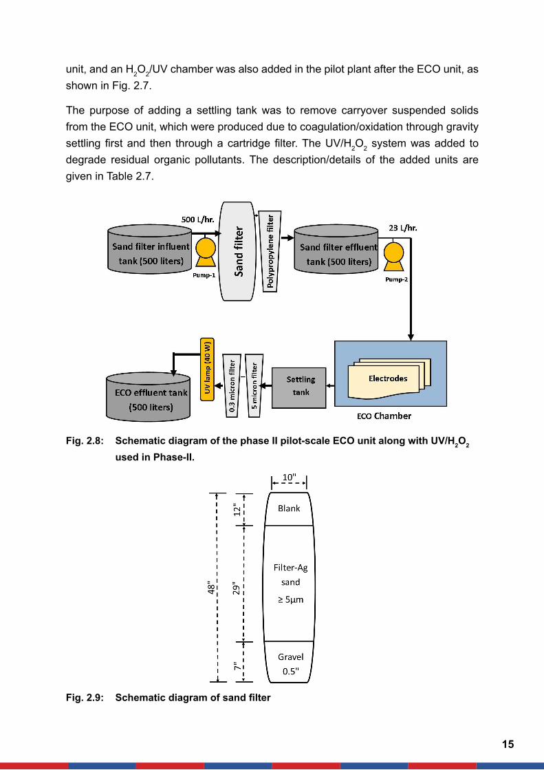
The purpose of adding a settling tank was to remove carryover suspended solids from the ECO unit, which were produced due to coagulation/oxidation through gravity settling first and then through a cartridge filter. The UV/H2O2 system was added to degrade residual organic pollutants. The description/details of the added units are given in Table 2.7.

Fig. 2.8: Schematic diagram of the phase II pilot-scale ECO unit along with UV/H2O2 used in Phase-II.

Fig. 2.9: Schematic diagram of sand filter

16

Table 2.6: Specification and dimensions of the sand filter and cartridge filter used prior to the ECO system.

Item Specifications/details

Sand filter (SF)

Sand filter casing 10-inch dia, 48 inches in total length

Media in sand filter

Gravel (0.5 inches): filled up to 7 inches from the bottom of the casing

Sand (Filter-Ag plus): 29 inches from the top of the gravel layer

Empty space: 12 inch

Physical properties of sand

Dry Bulk Density: 50 lb/cubic feet,

Specific Gravity: 2.2 g/cubic centimeter

Mesh Size: 14x30

Effective Size: 0.55 mm

Uniformity Coefficient: 1.8

Hardness: 4-5 (Mohs Scale)

Operating conditions of SF

Operating pressure: 10-15 psi

Backwash pressure: 30 psi

Max. flow rate/backwash rate: 500 L per hr/700 L per hour

Frequency of backwash: once in three days for 15 min

Cartridge filter

Dimensions 0.51m (length) × 0.0635 m (dia)

Operating conditions

Max. pressure 100 psi

Operating pressure: 30-50 psi

Flow= 23 L/hr

Surface area of the filter =0.1014 m2

Flux: 226.93 L/m3.hr

17

Table 2.7: Details of the units added after the ECO unit in Phase-II.

Item Specification/details

Settling tankVolume: 80 LitersRetention time: 3.47 hr

Holding tank 50 Liters

Cartridge filter after settling tank

No.: Two in series1st cartridge: 5 µm openings [0.254 m (length) x 0.057 m (dia)]2nd cartridge: 0.35 µm openings [0.254 m (length) x 0.057 m (dia)]Material: Polypropylene

UV/H2O2 unit

UV lamps

Type: Low-pressure low-intensity UV lamp

Irradiation wavelength: 256 nm

Model: Philips, TUV 36T5 HE 4P DE

Nos.: Two

Power: 40 W

Dimensions: 845.4 mm length x 19.3 mm dia

Volume of UV chamber: 5 Liter

Retention time in the UV chamber: 13 minutes

H2O2 dosingH2O2 pumping: 3-4 liter/hr

H2O2 content: 34.5%

2.10 Operation of Pilot-scale ECO unit

In Phase I, the pilot-scale ECO unit was operated in which shrimp processing wastewater was used as the influent to the sand filter. After sand filtration, the sand filter effluent was fed to the ECO chamber at the flow rate of 80 L/hr. In the ECO chamber, two different current densities were supplied to the electrodes, i.e., 56.4 A/m2 and 76.9 A/m2 in different time intervals, and treatment efficiency in terms of COD was observed. Afterward, the ECO chamber was operated at flow rates of 23 L/h and 15 L/h with a current density of 112.8 A/m2. In the last stage, the effluent of ECO was filtered with a 120-µm polypropylene filter.

18

In Phase II, the pilot-scale ECO was also operated at the industry with added units of filtration and UV/H2O2. The flow rate of the influent wastewater in the ECO chamber was kept at 23 L/h. In the ECO chamber, the current density of 112.8 A/m2 was fixed at the electrodes. The ECO effluent was discharged to the settling tank for HRT of 3.47 hr. Moreover, the effluent of the settling tank was dosed with H2O2 dosing before irradiation with UV light in the UV chamber. The operational parameters for the pilot-scale ECO unit during Phase I and Phase II are shown in Table 2.8. The pilot-scale ECO unit operated in the industry is shown in Fig. 2.10. In both phases, the samples were collected in 500 ml sterilized glass bottles for influent of sand filter, electrocoagulation influent and treated water and sample were analyzed in the laboratory for the pH, TDS, COD, TN, TP, NO3, color, turbidity, and PO4 according to the standard methods (APHA, 2012).

Table 2.8: Operating parameters of the ECO unit at the pilot-scale.

Operational parameters Units ECO/UV chamber

ECO chamber

Flow rate L/hr 80, 23, 15

HRT hr 1, 3.2, 5.3

pH 6.5-7.5

ECO chamber volume L 105

Current densities A/m2 56.4, 76.9, 112.8

Electrode surface area ft2 21

UV chamber

Flow rate L/hr 23

Volume of UV chamber Liters 5

No of lamps 2

Power/UV lamp Watts 40

H2O2 dosing ml/L 1, 1.5

2.11 Cost-benefit Analysis

The treatment efficiencies of the two operating systems were evaluated based on organic pollutants (COD) and particulate matter (TSS) removals. The best treatment

19

ECO Settling tank

H2O2 dosing tank

UV chamber

Sand filter

Influent tank of

Sand filter

Effluent of Sand filter &

Influent of ECO

Cartridges (5 and 0.3

micron)

Cartridge filter (5micron)

Fig. 2.10: ECO unit installed at the facility for the treatment of shrimp processing wastewater

scheme was selected for comparison of cost-benefit analysis (CBA) with a reverse osmosis (RO) system for desalination of groundwater of the same capacity (cost/m3 of produced water).

Phase III

In the third phase, an environmental study was conducted to quantify the environmental impacts caused by shrimps’ processing by performing a life cycle assessment of a selected shrimps processing facility. This study aimd to compare the environmental damages caused by the current processing system and those with the addition of wastewater treatment and water reuse systems in the existing processing system.

2.12 Environmental Impacts using Life Cycle Assessment

Life-cycle assessment is an analytical tool that is used to quantify the environmental burdens of a product or process throughout its life cycle from the cradle to the grave. Product or process lifecycle means all the life stages of the process, which include the extraction of raw material, production, transportation, use, and disposal (Kuczynski et al., 2012). Aktan and Salih (2006) reported standardized LCA methodology that was used to evaluate the environmental burdens. This methodology comprised four phases: 1) goal and scope definition, 2) life-cycle inventory, 3) life-cycle impact assessment, and 4) interpretation of results.

20

2.12.1 Goal and scope of the impact assessment through LCA

It is necessary to define the system to be studied, and the purpose of the study is also defined before conducting a life cycle assessment. System boundaries are chosen, i.e., cradle-to-grave, cradle-to-gate, and gate-to-gate. The functional unit of the product is decided based on all the calculations, and analysis is carried out.

The goal of the current study was to evaluate the environmental impacts and ecosystem damages caused by the activities involved in the processing of the raw shrimps. The functional unit (basic unit of product used to quantify the impacts) is one ton of raw shrimps. Three sub-systems of the shrimps’ product life cycle were taken into consideration, i.e.,, transportation of raw shrimps from the harbor to the industry gate, electricity production, and the processing of shrimps, for estimation of the environmental impacts of the final product.

2.12.2 Life cycle inventory

This phase of the LCA study consists of the collection and organization of data about the processes, resource use, energy consumption, emissions, and product of by-products resulting from the activities involved in the product life cycle. The production chain or system studied can be divided into two systems, i.e., foreground system and background system.

The data were gathered through field visits, interviews with workers, industry management, and authorities at the fish harbor. Some secondary data were also used to quantify the impacts.

1. Transportation data: This process involved the supply of raw shrimps from the fish harbor to the industry gate with the help of a compressed natural gas (CNG) powered vehicle (Suzuki), which carries around 800 kg raw shrimps per round. The distance covered by the vehicle was about 3 km to the industry gate. The other data related to the CNG consumption and emissions were taken from the SimaPro database (Ecoinvent).

2. Processing data: This stage involved various steps to transform raw shrimps into a final product for export. The data related to input and output was collected from the industry, hands-on measurement, and the literature. Only water and energy inputs were considered for environmental damage assessment, as shown in Table 2.9. Chemicals, packaging materials, and the electricity consumed for refrigeration were neglected due to the unavailability of data.

3. Electricity production: The data related to energy production were collected from SimaPro databases. The energy production data were organized

21

according to the total energy production from different sources in Pakistan. For this purpose, a new process was set, which included the production of electricity from different processes. Data related to these processes were collected from the database.

Table 2.9: Inventory data of the shrimps processing per kg of raw shrimps processed.

Inputs

Component Unit Quantity

Raw shrimps Kilogram 1

Freshwater Liters/ kilogram 6.125

Groundwater consumption (for floor-cleaning)

Liters/day 20,250

Electricity (for 3000 kg shrimps)

Kilowatt-hours/Kilogram

0.013 (excluding consumption by

refrigeration)

Outputs

Packed shrimps Kilogram 1

Wastewater Liters/ kilogram 5.7

Emissions to water bodies

Chemical oxygen demand (COD)

Gram/kilogram 34.02

Total phosphorus (TP) Gram/kilogram 0.69

Total nitrogen (TN) Gram/kilogram 4.42

2.12.3 Life cycle impact assessment

Life cycle impact assessment (LCIA) aimed at understanding and evaluating of the potential environmental impacts caused by the product through its life cycle stages. This phase involves quantification, assessment, and interpretation of potential environmental impacts caused by the product through the characterization of product flows. LCIA is carried out in different steps, which are the classification of emissions into different impacts categories, characterization of the midpoint, and damage (endpoint) characterization.

Environmental impacts were estimated using a user-friendly life-cycle assessment software SimaPro. Two scenarios were run (Fig. 2.11).

22

Fig. 2.11: Scenarios for wastewater treatment and environmental damages

Wastewater

Treatment

Environmental

Damages

Shrimps

Processing

Industry

Water Use

and

Wastewater

Water Use and

Wastewater

Shrimps

Processing

Industry

Environmental

Damages

Water Reuse

Scenario 1

Scenario 2

1. Processing with direct disposal of wastewater in the ocean: It was considered that there wasn’t any wastewater treatment and water reuse at the processing plant; the wastewater was directly discharged into the sea.

2. Processing with the addition of a wastewater treatment system and water reuse: The wastewater treatment system was introduced, and the treated water was reused within the facility.

Several assumptions were made, such as electricity needed to process 1 kg of shrimps produced from various processes developed in the SimaPro databases. The freshwater used was considered to be from a lake in Pakistan. For scenario 2, it was assumed that the treated water would be used for cleaning of the floor, which would alternatively reduce the groundwater consumption by 50 percent.

The impact assessment method ILCD 2011+ midpoint was used to study 10 environmental impacts categories. The impacts are categorized for midpoint impacts, i.e., climate change, ozone depletion, particulate matter, freshwater eutrophication, marine eutrophication, water resource depletion and mineral, fossil and renewable resource depletion (Snaidr et al., 1997; Ahmed et al., 2008)

2.13 Best Management Practices

2.13.1 Pollution reduction by screening

The screening tests for the wash-water of cleaning and soaking processes were performed by 600 µm and 200 µm screens, respectively, at the facility to reduce the number of coarse particles and objects in the effluent (Fig. 2.12). This screening

23

practice from washing and soaking processes showed the removal of coarse material (pieces of organics, solids). There was a reduction in pollutants’ concentrations in both processes when effluents were analyzed after screening.

Fig. 2.12: Washing and soaking processes’ effluents screening

2.13.2 Segregation of drainage points

The shrimp processing industry has two sources of freshwater, e.g., tanker water and groundwater. The tanker water is utilized in shrimp processing like the washing, soaking, and screening process, and it generates the contaminated wastewater, whereas the groundwater is used in the cleaning of the floor after processing. The drains points of effluent discharge should be covered with labeled rubber plugs for shrimp processing wastewater and groundwater separately. During shrimp processing (SP), water would be drained, and all other groundwater (GW) drain plugs will be closed. If groundwater is used for floor flushing, then all other shrimp processing drains would be closed, while the groundwater plug remains open.

2.13.3 Schedule/work plan of the project

As mentioned earlier, the project activities were performed in three phases. The breakup of activities is given in Table 2.10.

24

Table 2.10: Schedule/work plan of the project

PhaseDuration (Months)

Description

I 3

Survey of processing unit

Identification of sampling points

Sampling and analysis of freshwater and wastewater

Quantification of freshwater and wastewater

II 8

Fabrication of SAAM

Fabrication of ECO

Operation of SAAM

Operation of ECO

Analysis of influent and effluent samples of SAAM and ECO

Estimation of pollutant discharge

III 4

Life cycle inventory

Impact assessment

Report writing

Paper writing

25

3. RESULTS AND DISCUSSION3.1 Quantification of Freshwater Utilization

The water utilized in washing, soaking, cleaning, and packing process of the facility was 3.42, 1.53, 0.75, and 0.425 L/kg of shrimps, respectively (Fig. 3.1). The water used and the wastewater generated showed similar results because the same inlet and outlet were estimated from each processing step of the industry. The industry uses tanker water for shrimp processing, and its use fluctuates with the production of shrimps. The water quantity was determined for three production levels, low production, regular production, and maximum production of shrimps. In low production, the average shrimp production was estimated as 3,000 kg/d, and 10,260 L/d water was used for cleaning and washing of shrimps. Furthermore, the water utilization was 27,562.5 L/d and 36,750 L/d in regular (4,500 kg/d) and maximum shrimp production (6,000 kg/d), respectively.

Fig. 3.1: Water utilization in shrimps processing

Washing 56%Soaking

25%

Peeling12%

Packing7%

3.2 Characterization of Freshwater Consumed

Water samples from the water tanker and groundwater were characterized for pH, TDS, chloride, and sulfate. The pH of tanker water was in the range of 7.25-7.8, while the groundwater pH ranged from 7.18 to 7.28. The tanker water used for shrimp processing had an average TDS of 2,077 mg/L, whereas groundwater had a high TDS value of 31,567 mg/L. The complete results of the water quality are shown in Table 3.1.

26

Table 3.1: Characteristics of freshwater used in the shrimp processing facility

Parameter*Sample

Tanker water Groundwater

pHRange 7.25-7.80 7.18-7.28Average(n) 7.52(3) 7.24(3)

TDSRange 2000-2140 31000-32500Average(n) 2076.7(3) 31566.7(3)

ChlorideRange 500-602 12900-19852Average(n) 551(2) 16376(2)

SulfateRange 270-300 675-750Average(n) 285(2) 712.5(2)

• All values are in mg/L except pH, n= number of samples

3.3 Characterization of the Wastewater from the Facility

The samples were taken from the washing and soaking processes, septic tank, and effluent of the facility and analyzed for pH, TDS, COD, BOD, TN, TP, chloride, and sulfate. The pH serves as one of the crucial parameters because it may reveal contamination of wastewater by ammonia or indicate the need for pH adjustment for the biological treatment system to function. The average pH from the above sampling points was obtained to be 7.36, 7.72, 7.27, and 7.40, respectively (Appendix 1). Mostly, the pH was found to be neutral. The pH levels generally reflect the decomposition of aqueous protein matter and the emission of ammonia compounds. Solids content in wastewater can be divided into dissolved solids and suspended solids. However, suspended solids are the primary concern since they are objectionable for several reasons. The TSS and VSS concentrations from washing, soaking, septic tank, and industry drain were obtained as 2,483, 682, 12,490 and 1,253 mg/L and 1,952, 635, 6,199, and 894 mg/L, respectively (Fig. 3.2).

0

3000

6000

9000

12000

15000

Washing Soaking Septic Tank Industry drain

Solid

s (m

g/L)

Total suspended solids (TSS)

Volatile suspended solids (VSS)

Fig. 3.2: TSS and VSS concentration in different streams

27

The TDS of the four shrimp processing steps were determined to be 4,199, 4,503, 10,929, and 7,281 mg/L, respectively (Fig. 3.3).

Fig. 3.3: TDS of shrimp processing wastewater

0

3000

6000

9000

12000

15000

Washing Soaking Septic tank Industry drain

TDS

(mg/

L)

Biochemical oxygen demand (BOD) estimates the degree of contamination by measuring the oxygen required for the oxidation of organic matter by aerobic metabolism of the microbial flora. In the shrimp processing wastewaters, this oxygen demand originates mainly from two sources: carbonaceous compounds that are used as a substrate by the aerobic microorganisms and the nitrogen-containing compounds that are normally present in the shrimp processing wastewaters, such as proteins, peptides, and volatile amines. Standard BOD5 tests were conducted at 5-day incubation for the determination of BOD5 concentrations. Wastewaters from shrimp processing operations can be very high in BOD5. The average BOD5 of shrimp processing steps of washing, soaking, septic tank, and industry drain were obtained as 3462, 3325, 10423, and 2683 mg/L, respectively (Fig. 3.4). The filtered BOD5 (BODf) was also performed by filtering the

Fig. 3.4: BOD of shrimps processing wastewater

0

2000

4000

6000

8000

10000

12000


BO

D (m

g/L)

BODt

BODf

28

samples with a 0.45-micrometer glass filter paper. BODf from the four sampling points were in the range of 2621, 2839, 3476, and 1511 mg/L, respectively.

Another alternative for measurement of the organic content in wastewater is the chemical oxygen demand (COD), an important pollutant parameter for the shrimp processing industry. This method is more convenient than BOD5 since it needs only about 2.5 hours for its determination compared to 5 days for BOD5 determination. In COD analysis, the number of compounds that can be chemically oxidized is greater than those that can be degraded biologically; hence, the COD of a sample is usually higher than the BOD5. Depending on the types of seafood processing, the COD of the wastewater can range from 150 to about 42,000 mg/L. The average COD of washing, soaking, septic tank, and effluent of industry were recorded as 7843, 5738, 18834, and 5917 mg/L, respectively. And the average filtered COD (CODf), after filtering the sample through a 0.45-micrometer glass filter paper, were obtained as 4445, 4284, 8789, and 4151 mg/L, respectively (Fig. 3.5).

Fig. 3.5: COD of shrimps processing wastewater

0

4000

8000

12000

16000

20000


CO

D (m

g/L)

CODt

CODf

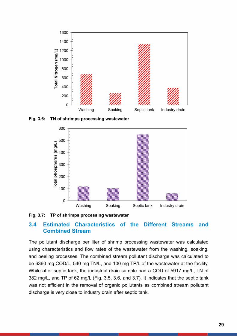
Excessive concentration of nitrogen and phosphorus can cause adverse environmental impacts. It may cause the proliferation of algae and affect aquatic life in a water body if they are present in excess. Their concentration in the shrimp processing wastewater is a concern in most cases. It is recommended that a ratio of N to P of 5:1 be achieved for the proper growth of the biomass in the biological treatment (Manz et al., 1996; Bankhead, 2014). The average total nitrogen (TN) and total phosphorus (TP) concentrations from washing, soaking, septic tank, and effluent of industry were obtained as 680, 260, 1,350 and 380 mg/L (Fig. 3.6) and 119, 105, 551 and 62 mg/L (Fig. 3.7), respectively. Moreover, chloride and sulfate concentrations from washing, soaking, septic tank and effluent of industry were found to be 1586, 1849, 5151, and 2941 mg/L and 332, 255, 462, and 287 mg/L, respectively, as presented in Appendix 1.

29

3.4 Estimated Characteristics of the Different Streams and Combined Stream

The pollutant discharge per liter of shrimp processing wastewater was calculated using characteristics and flow rates of the wastewater from the washing, soaking, and peeling processes. The combined stream pollutant discharge was calculated to be 6360 mg COD/L, 540 mg TN/L, and 100 mg TP/L of the wastewater at the facility. While after septic tank, the industrial drain sample had a COD of 5917 mg/L, TN of 382 mg/L, and TP of 62 mg/L (Fig. 3.5, 3.6, and 3.7). It indicates that the septic tank was not efficient in the removal of organic pollutants as combined stream pollutant discharge is very close to industry drain after septic tank.

Fig. 3.6: TN of shrimps processing wastewater

Fig. 3.7: TP of shrimps processing wastewater

0

200

400

600

800

1000

1200

1400

1600


Tota

l Nitr

ogen

(mg/

L)

0

100

200

300

400

500

600


Tota

l pho

spho

rus

(mg/

L)

30

Moreover, the combined stream TDS was 4045 mg/L, and after septic tank, the industry drain had a TDS of 7281 mg/L. It indicates that the industrial drain had a high TDS than combined stream TDS due to the addition of groundwater in septic tank by flushing the floor of the shrimp processing industry. The pollutant discharge of COD and BOD was also calculated after filtration through 0.45 µm filter, and it had reduced the COD from 6360 to 4400 mg/L and BOD from 3250 to 2690 mg/L (Table 3.2).

Table 3.2: Calculation of pollutant discharge per liter of shrimps processing wastewater

Parameter* Washing Soaking PeelingCombined

stream

COD 7,843 5,738 900 6,360

CODf 4,445 4,284 --- 4,400

BOD 3,462 3,325 350 3,250

BODf 2,621 2,839 --- 2,690

TN 680 260 60 540

TSS 2483 682 160 1529

VSS 1982 635 95 1372

TP 119 105 10 100

TDS 4,199 4,503 2,410 4,045

Flow rate 20,520 9,180 4,500 34,200

• All values are in mg/L, except flow rate in L/d

Besides, the pollutant generation per kg of raw shrimp processing was calculated from different streams and combined streams. The combined pollutant generation from washing, soaking, and peeling processes were 36.3 g COD/kg, 17.2 g BOD/kg, 2.8 g TN/kg, and 1.1 g TP/kg of raw shrimp production at the facility (Table 3.3). Whereas, the washing process in shrimp processing generated 26.8 g COD/kg, the soaking process generated 8.8 g COD/kg, and the peeling process generated 0.68 g COD/kg of shrimp production. Complete results are shown in Table 3.3.

Table 3.3: Pollutant discharge per kg of shrimp production

Parameter* Washing Soaking Peeling Combined streams

COD 26.8 8.8 0.68 36.3

BOD 11.8 5.1 0.26 17.2

TN 2.3 0.4 0.05 2.8

TP 0.9 0.2 0.01 1.1

• All values are in g/kg of shrimp

31

Furthermore, the lab experiment was performed to determine the characteristics of different streams and combined streams by taking 50 grams of raw shrimp. The combined streams generated 59.4 g COD/kg of shrimp. When compared to pollutant generation at the facility, it indicated that the lab experiment generated relatively high COD than that by the facility because the industry utilizes a higher volume of freshwater; consequently, lower concentrations appear in the effluent. The filtered samples from the washing and soaking processes were also analyzed for CODf, which came out to be 53.5 g/kg of shrimp. The purpose of analyzing CODf was to observe the reduction in pollutants after filtration, which was found to be 9.9%.

3.5 Treatment of Shrimp Processing Effluent using SAAM

In Phase I, the SAAM was operated with synthetic wastewater at CODs of 2,000 mg/L and 3,000 mg/L. In Phase II, the SAAM was operated with a mixed ratio of synthetic and industrial wastewater with a COD of 3,000 to 4,000 mg/L. Lastly, in Phase III, the SAAM was operated with pure industrial wastewater at a COD in the range of 4,000-6,000 mg/L. The complete phases of bench-scale SAAM are shown in Table 3.4.

The SAAM influent and effluent samples were analyzed for pH, TDS, COD, TN, TP, NO3

--N, and (PO4)3--P. The pH data are generally used to determine whether a process

is operating within the acceptable range of 6.5-7.5 for the biological treatment system to function. The results showed that the pH of feed and effluent were 7.49±0.395 (n= 166) and 7.93±0.458 (n= 166), respectively. It indicated that the pH value of SAAM effluent was in the range of 6-9, according to NEQS, as shown in Appendix 2. The average COD, TN, and TP removal were achieved to be 94.3, 69.5, and 53.3%, respectively, throughout the study period. Dissolved organic carbon (DOC), NO3

--N and (PO4)3--P

were reduced by 96.8, 61.7, and 94.3%, respectively. The SAAM treatment had no considerable effect on the TDS concentrations in the effluent. The complete results are shown in Table 3.5.

32

PhaseDuration (Days)

Feeding sourceOLR

(g/l/day)Description

I15 Synthetic wastewater 5.4

Stabilization of SAAM on synthetic wastewater (2000±14 mg/L)

28 Synthetic wastewater

8.1

Stabilization of SAAM on synthetic wastewater (3000 mg/L)

II

7Synthetic wastewater + shrimp processing wastewater (90%+10%)

10% of the total COD (3000 mg/L) comprised of shrimp processing wastewater






60% of the total COD (3000±14 mg/L) comprised of shrimp processing wastewater



18Synthetic wastewater was replaced with shrimp processing wastewater

SAAM was operated on 2 × diluted shrimp processing wastewater (COD 3000 mg/L)

20 Shrimp processing wastewater 10.91.5 × diluted shrimp processing wastewater (COD

4000±330 mg/L)

III40 Shrimp processing wastewater 10.9

1.5 × diluted shrimp processing wastewater (COD 4000±330 mg/L)

9 Shrimp processing wastewater (100%) 16.3Shrimp processing wastewater COD (6000±253

mg/L)

Table 3.4: Phases of bench-scale SAAM operated in laboratory

33

Table 3.5: Treatment of the shrimp processing effluent before and after SAAM treatment

Para

met

er* SAAM influent SAAM effluent Removal

Range Mean ± STD(n) Range Mean ± STD(n) %

pH 6.57-8.72 7.49±0.395(166) 6.73-8.92 7.93±0.458(166) ---

TDS 1,531-9,490 5,547±2049(166) 1,270-8,480 5,151±1,929(166) ---

COD 1,500-6,790 3,548±1,045(166) 22-1,274 201±211(166) 94.3

TN 92-659 524±164(20) 18-265 160±57(20) 69.5

TP 22-180 165±57(24) 3.1-100 77±29(24) 53.3

DOC 947-1666 1153±291(5) 25-50 37±11(5) 96.8

NO3- 188.6-289.7 235±26(14) 65.9-133 90±21(14) 61.7

(PO4)3- 343-808 598±132(21) 15-88.5 34±25(21) 94.3

• All values are in mg/L except pH

3.6 MLSS and MLVSS Concentration in Anoxic/Anaerobic and Aerobic Reactor

The concentration of MLSS and MLVSS in the anaerobic and aerobic reactors is shown in Fig. 3.8 and 3.9, respectively. During Phase-I, the concentration of MLSS and MLVSS decreased, followed by a lag phase characterized by a period of adaptation of microorganisms to the SAAM process and the synthetic effluent. In Phase II, the SAAM

Fig. 3.8: MLSS and MLVSS concentration in the aerobic reactor

0

2000

4000

6000

8000

10000

12000

14000

16000

10 26 42 58 71 83 92 104 117 129 144 162

Solid

con

cent

ratio

n, m

g/L

Time (Days)

TSS concentrationVSS concentration

34

was operated with different proportions of synthetic wastewater and shrimp processing effluent. The reactor SRT was set to 60 days. During phase II, the concentration of MLSS and MLVSS raised gradually due to the enormous amount of MLSS in the shrimp processing effluent. During Phase III, the recycling ratio of SAAM was set to 3 times the influent flow rate. In this period, the MLSS and MLVSS concentrations were higher than those in Phase II.

3.7 TDS Concentration in Influent and Effluent of SAAM

In Phase I, the SAAM was operated at 2,000 and 3,000 mg COD/L at synthetic wastewater. The average influent and effluent TDS were 3,012 and 2,689 mg/L, respectively. In Phase II, the SAAM was operated at a mixed ratio of synthetic wastewater and industrial wastewater from 3,000 to 4,000 mg COD/L. During this phase, the average influent and effluent TDS were increased to 4,870 and 4,674 mg/L, respectively, due to the addition of (NH4)2SO4 (Daejung, Korea) salt as a nitrogen source. In Phase III, the average influent and effluent TDS were also increased to 8,184 and 8,023 mg/L, respectively (Fig. 3.10) when the SAAM was operated with the industrial wastewater with COD 4,000 to 6,000 mg/L. The wastewater was high in nitrogen concentration and salt content. The effluent TDS concentration of SAAM was higher than the national environmental quality standards (NEQS) limit, as shown in Appendix 2.

Fig. 3.9: MLSS and MLVSS concentration in the anoxic/anaerobic reactor

0

2000

4000

6000

8000

10000

12000

14000

10 26 42 58 71 83 92 104 117 129 144 162

Solid

con

cent

ratio

n, m

g/L

Time (Days)

TSS concentrationVSS concentration

35

Fig. 3.10: TDS concentration in influent and effluent of SAAM

0

2000

4000

6000

8000

10000

0 10 20 30 40 50 60 70 80 90 102 112 122 132 142 152 162

TDS

(mg/

L)

Time (days)

TDS influentTDS Effluent

Phase I Phase II Phase

3.8 Removal of COD in SAAM

The SAAM was operated at different operational conditions, including COD, internal recycle ratio, and SRT. The HRT of 5.4 hours was kept throughout the experimental run of the SAAM. Phase I, which started from day 1 to day 43, being the acclimatization period for the SAAM. From day 1 to 20, the SAAM was operated with synthetic wastewater with a COD of 2,000 mg/L, whereas the pH of the system was maintained from 7.5 to 8.5. The main source of synthetic feed was glucose and sodium acetate. The efficiency of the system was recorded as 65% on the very 1st day, which increased to 98% until the 19th and 20th days. After the 20th day, the COD of synthetic wastewater was increased to 3000±300 mg/L. The efficiency of the system remained stable until the 20th day of operation. However, it dropped to 61% on day 21. The efficiency loss was mainly due to the improper handling of the system. The reactor has overflown mistakenly, and dissolved oxygen (DO) was also very low. Due to the overflowing of the reactor, some quantity of sludge was wasted, and the reactor became unstable. After a few days, it was stabilized again. On day 35, the efficiency improved again to 96% and remained at that level, as shown in Fig. 3.11. The COD removal efficiency was obtained as 90% at a recycling ratio of 2.5×Qi (2.5 times the influent flow rate) during Phase I.

In Phase II, the reactor feed was gradually transferred from synthetic wastewater to the shrimp processing wastewater after the acclimatization of the reactor on the synthetic wastewater. The SRT of the reactor was set to 60 days. Initially (from day 44 to day 97), the SAAM was operated at 3,000 mg COD/L with a mixed ratio of industrial wastewater and synthetic wastewater. It was started with a mixed ratio of industrial wastewater: synthetic wastewater of 1:9, then sequentially changed to 2:8, 4:6, 6:4, 8:2, and 10:0. The COD was changed to 4,000 mg/L when the recycling ratio was kept

36

Fig. 3.11: COD concentration in influent and effluent of SAAM

0

1000

2000

3000

4000

5000

6000

7000

8000

0 10 20 30 40 50 60 70 80 90 102 112 122 132 142 152 162

CO

D (m

g/L)

Time (days)

COD influentCOD Effluent

Phase III

Syntheticwastewater

Mixed synthetic wastewater+Industrial

wastewater

Diluted industrial

wastewater

10%

20%

40%

60%

80%

100%

at 2.5×Qi up to 117th day of operation. In Phase I, and Phase II, the recycling ratio of SAAM was maintained at 2.5×Qi. The highest COD removal was obtained as 97% at a mixed ratio of 2 parts of the industrial wastewater and 8 parts of the synthetic wastewater. In Phase III, the SAAM was operated with the industrial wastewater with a COD of 4,000 and 6,000 mg COD/L (from day 118 to day 166) at a recycling ratio of 3.0×Qi for which the removal efficiency was 93.5% and 95%, respectively. The effluent COD concentration of SAAM was lower than the NEQS limit, as revealed in Appendix 2 throughout the operational period of SAAM.

3.9 Removal of TN and TP in SAAM

TN and TP removals were 68% and 51.5% at a recycling ratio of 2.5Qi, as shown in Fig. 3.12 and Fig. 3.13. When the SAAM was operated at the recycling ratio of 3.0 Qi, the TN and TP removals increased from 68 to 71.8% and from 51.5 to 57.6%, respectively. Nitrogen and phosphorus are the nutrition sources for microorganisms, which they can partially remove from wastewaters. The higher nitrogen removal was observed due to nitrification and denitrification in the SAAM. The increase in TP removal was achieved because of the presence of phosphorus accumulating microorganisms and excess sludge withdrawal from the anoxic tank. The NO3

- and (PO4)3- removal efficiencies

were also monitored during Phase III of the SAAM operation. The average NO3 and

(PO4)3- removal were obtained as 64% and 94%, respectively.

The results of SAAM indicated that the effluent water is under the limit when compared to NEQS guideline values except for the effluent TDS value.

37

Fig. 3.12: TN concentration in the influent and effluent of the SAAM

0

100

200

300

400

500

600

700

46 66 86 106 126 146 166

TN (m

g/L)

Days

TN InfluentTN Effluent

0

50

100

150

200

46 66 86 106 126 146 166

TP (m

g/L)

Days

TP InfluentTP Effluent

Fig. 3.13: TP concentration in the influent and effluent of the SAAM

3.10 Fluorescence in-situ Hybridization

Fluorescence in situ hybridization was performed to observe the relative abundance of various groups of bacteria using the EUB338 probe for targeting the eubacterial group and seven other probes based on their specificity. The total population counter-stained with 4′,6-diamidino-2-phenylindole DAPI detected 92% cells hybridized with EUB338 probe – targeting eubacterial group. Microscopic results revealed the presence of filamentous, rod-shaped, and round-shaped bacteria. The hybridization was performed under optimal conditions; each slide, hybridized with a specific probe observed under the fluorescence microscope, revealed the proportion of each targeted group of bacteria in the microbial community of MBR.

The population of different classes was investigated. The results showed that among the total bacterial, population of α-proteobacteria reduced from 13.2% in the initial stage

38

and 7.8% in final stage, β-proteobacteria increased from 9.3 to 11.31%, γ-proteobacteria reduced from 9.7 to 3.4%, population of sulfur-reducing bacteria elevated from 4.6 to 18.1%, Halotolerant bacteria increased from 2.5 to 5.6%, Actinobacteria increased from 3.7 to 11.8% and Cytophaga-flavobacteria decreased from 12 to 2.7%. The unidentified population in the community was 44.57% in the initial stage and remained 39.1% in the final stages (Table 3.6).

All cells of the sludge samples were stained with 4′,6-diamidino-2-phenylindole, a blue fluorescent DNA dye, observed under an Epifluorescence microscope (Carl Zeiss Microscopy Axio Scope.A1 GmbH Germany) through EC plan-Neoflaur 10X lens and captured by software ZEN 2.5 blue edition. A monograph of all stained cells with DAPI is shown in Fig. 3.14.

Table 3.6: Results from fluorescence in-situ hybridization demonstrated in the initial and final stage on MBR

S # Type of bacteria % in the initial stage % in the final stage1 α-Proteobacteria 13.2 7.8

2 β-Proteobacteria 9.3 11.31

3 γ-Proteobacteria 9.7 3.4

4Various δ-Proteobacteria (sulphur reducing bacteria)

4.6 18.1

5Cytophaga– flavobacteria cluster

12 2.7

6 Halotolerant bacteria 2.5 5.6

7Actinobacteria (Gram-positive bacteria with high G+C content of DNA)

3.7 11.8

8 Unidentified 44.57 39.1

Graphical representation of microbial community dynamics showing distribution and changes in the population, hybridized with oligonucleotide probes: Alf1b (α-Proteobacteria), Bet42a (β-Proteobacteria), Gam42a (γ-Proteobacteria), SRB385 (Sulphur reducing bacteria), NEU653 (Halotolerant bacteria), HGC69a (Actinobacteria), CF319a (Cytophaga flavobacteria), in initial and final stage of Membrane Bioreactor, as shown in Fig. 3.15, observed by fluorescence in situ hybridization (FISH) technique. The population of different classes is shown in Fig. 3.16 to Fig. 3.21.

39

Initial Stage Final Stage0

20

40

60

80

100

Relat

ive a

bund

ance

%

Operating stages of an MBR

Unidentified Bet42a Gam42a HGC69a CF319a NEU653 SRB385 Alf1b

Fig. 3.15: Graphical representation of microbial community dynamics showing distribution and changes in the population, hybridized with oligonucleotide probes

Fig. 3.14: DAPI stained cells in the sludge samples from the membrane bioreactor

40

Fig. 3.16: Relative abundance of β-Proteobacteria

Fig. 3.17: Relative abundance of α-Proteobacteria

41

Fig. 3.19: Relative abundance of δ-Proteobacteria

Fig. 3.18: Relative abundance of γ-Proteobacteria

42

Fig. 3.20: Relative abundance of Actinobacteria

Fig. 3.21: Relative abundance of Cytophaga-Flavobacteria cluster

3.11 16s rRNA Metagenomic Sequencing

The taxonomic profile of microbiota in MBR presented total reads of 107,425,094 (in the initial stage) and 97,626,942 base pairs (bps). The total number of sequence reads was 356,894 in the initial stage, and 324,342 in the final stage. The results from the phylum level to genus level are described below:

43

3.11.1 Phylum-level

In the initial stage, Fusobacteria (38%) remained dominant phylum. The second and third phyla TM7 (36%) and Proteobacteria (18%) and Firmicute (3%) was a rare phylum. The predominant phylum during the final stage was TM7 (36%). The second, third, and fourth major phyla were Firmicutes (17%), Proteobacteria (14%), and Bacteroides (13%), respectively. The rare phyla were WS6 (1%), Planctomycetes (1%), Chloroflexi (1%), and OD1 (5%) (Fig. 3.22).

Fig. 3.22: Phylum level of bacteria in the initial and final stage of SAAM


20

40

60

80

100

Rela

tive

abun

danc

e %

Operating stages of MBR

Unclassified Other WS6 TM7 Proteobacteria Planctomycetes OD1 Fusobacteria Firmicutes Chloroflexi Bacteroidetes

3.11.2 Class-level

A total of 46 classes were found from the initial and final stages. The class TM7-3 was 12% in the initial stage and showed a high abundance of 34% in the final stage. Five classes of phylum Proteobacteria; Alpha-Proteobacteria, Beta-Proteobacteria, Delta-Proteobacteria, Epsilon-Proteobacteria, Gamma-Proteobacteria were present with the abundance of 5, 2, 0.2, 1 and 10%, respectively, in the initial stage, and 4, 5, 2%, 1 and 2% in the final stage (Fig. 3.23).

3.11.3 Order-level

A total of 71 orders were detected. Among them, the dominant order in the initial stage was Fusobacteriales (38%). Other orders were found to be less prevalent and included Clostridiales (3%), Bacteroidales (6%), Rhodoacterales (4%), Burkholderials (2%), and Pseudomonadales (1%). In the final stage, I025 (sub-group of TM7) was present with high abundance, whereas 0.30% in the final stage. The second dominant

44

order in the final stage was Clostridiales (16%). Fusobacteriales were found with a huge difference in the final stage, 0.3%. The rest mentioned above had relatively the same concentration in the final stage, as shown in Fig. 3.24.


20

40

60

80

100

Rela

tive

abun

danc

e %

Operating conditions of MBR

Unclassified Other B142 Spartobacteria TM7-3 TM7-1 Gammaproteo Epsilonproteo Deltaproteo Betaproteo Alphaproteo Planctomycetia Fusobacteriia Clostridia Anaerolineae Saprospirae Flavobacteriia Bacteroidia Actinobacteria

Fig. 3.23: Class level of bacteria in the initial and final stage of SAAM

Fig. 3.24: Order level of bacteria in the initial and final stage of SAAM


20

40

60

80

100

Rela

tive

abun

danc

e %


unclassified Other Chthoniobacterales I025 Pseudomonadales Aeromonadales Campylobacterales Rhodocyclales Nitrosomonadales Burkholderiales Rhodobacterales Rhizobiales Fusobacteriales Clostridiales Caldilineales Saprospirales Flavobacteriales Bacteroidales

3.11.4 Family-level

At the family level, Peptostreptococcaceae (12%) and Clostridiaceae (7%) were at the top of 83 families in the final stage. In the initial stage, the dominant phylum was Fusobacteriaceae (38%). Flavobacteriaceae, Saprospiraceae, Caldilineaceae, Rhodobacteraceae, Comamonadaceae, Nitromonadaceae, Rhodocyclaceae, and Bdellovibrionaceae were found to be in very little amount, between 0-4% in both the stages as shown in Fig. 3.25.

45

3.11.5 Genus-level

At the genus level, 130 known genera were found. The most dominant genus at the genus level, in the initial stage, was Psychrilyobacter (38%). The core genera in the final stage of MBR were Proteocatella (8%) and Clostridium (5%). Other genera with less abundance found in the final stage of the MBR were Bdellovibrio (2%), Caldilinea (1%) and Nostocoida (1%) (Fig. 3.26). An average percent of the genus that remains unclassified is 61%.

Fig. 3.25: Family level of bacteria in initial and final stage of SAAM


20

40

60

80

100Re

lativ

e ab

unda

nce

%

Operating Stages of MBR

Unclassified Other Chthoniobacteraceae Sphaerochaetaceae Xanthomonadaceae Vibrionaceae Pseudomonadaceae Moraxellaceae Enterobacteriaceae Aeromonadaceae Campylobacteraceae Bdellovibrionaceae Rhodocyclaceae Nitrosomonadaceae Comamonadaceae Rhodobacteraceae Phyllobacteriaceae Fusobacteriaceae Peptostreptococcaceae JTB215 Clostridiaceae Caldilineaceae Saprospiraceae Chitinophagaceae Flavobacteriaceae Porphyromonadaceae Bacteroidaceae

Fig. 3.26: Genus level of bacteria in the initial and final stage of SAAM


20

40

60

80

100

Rela

tive

abun

danc

e %


Other Unclassified C xiphinematobacter Sphaerochaeta Pseudomonas Bdellovibrio Alkanindiges Aeromonas Helicobacter Georgfuchsia Azoarcus Nitrosomonas Psychrilyobacter Anaerorhabdus Succinispira Proteocatella Clostridium Caldilinea Macellibacteroides

46

3.11.6 Species-level analysis

16S rRNA metagenomic sequencing revealed only a small portion of the community on species level. Only 7% of the total reads from the initial stage and 15% from the final stage of MBR were detected. Among them, 100 species were detected with varying quantity, ranging from 2 to 6395. The most abundant among the known species was Proteocatella sphenisci (8%) in the final stage.

3.12 Biological Testing of Treated Effluent

The treated wastewater from the final stage was tested biologically twice a month during the operational period of SAAM. A 50 ml treated effluent was passed through 0.45 μm filter paper via membrane filtration assembly under sterilized condition. The filter paper was picked with sterilized forceps and put into solidified culture media plates of eosin methylene blue (EMB) – specific for total coliforms, and tryptone bile agar (TBA) – specific for Escherichia Coli. The plates were incubated at 37°C for 24 hours. Throughout the operation period, zero colony-forming units (CFUs) were detected in the effluent of the SAAM. While the PTFE membrane used in SAAM has a pore size of 0.45 µm that also removes all the bacteria from effluent water, this concludes that the treated water from the SAAM is free from fecal contamination.

3.13 Treatment of Shrimp Processing Effluent using ECO System

The electrocoagulation system was operated at different conditions, including current densities and HRT. The samples were collected from the sand filter influent, sand filter effluent, and treated water sample after the electrocoagulation process. These samples were analyzed at the Advanced Water Quality Lab of USPCAS-W, MUET. The sand filtration had a COD, TSS, TN, turbidity, and color removal of 8, 14, 6, 16, and 9%, respectively, whereas the electrocoagulation process had removal efficiencies of 39, 69, 31, 64, and 83%, respectively, in Phase I as presented in Table 3.7. It has been established that pH is an important operating factor influencing the performance of the electrocoagulation process (Ito et al., 2002; Baird et al., 2012; Huber et al., 2018). Generally, the pH of the medium changes during the electrocoagulation process (ISO, 2006; Vazquez-Rowe et al., 2012). This change depends on the type of electrode material and the initial pH. The pH of sand filter influent and effluent were 7.75 and 7.61, respectively, while the treated water sample from the ECO effluent had a pH of 8.33, which is slightly higher than the influent pH of the treatment process.

However, the TDS during the treatment process mostly remained the same. The average TDS of the sand filter influent, effluent, and ECO effluent were measured to be about 5,374, 5,274, and 4,604 mg/L, respectively. The treated water had a little drop in TDS value from 5,274 to 4,604 mg/L.

47

During Phase II of the system, the removal efficiencies for sand filtration were: 3% for COD, 13% for TSS, 4% for TN, 4% for DOC, 12% for turbidity, and 3% for color, whereas, electrocoagulation removal efficiencies were: 55% for COD, 98% for TSS, 30% for TN, 42% for DOC, 96% for turbidity, and 95% for color. In Phase II, it was noted that when electrocoagulation unit was operated along with the combination of UV/H2O2 reaction, the COD removal increased from 39 to 55%, while color removal increased from 83 to 95%, as shown in Table 3.8.

3.13.1 Removal of COD in the ECO process

In Phase I, electrocoagulation was operated at current densities of 56.4 A/m2 and 76.9 A/m2 with an HRT of 1 hr, and 112.8 A/m2 with HRTs of 3.3 and 5.3 hr. The COD removal was obtained at 49% at an HRT of 1 hr and a current density of 56.4 A/m2. When it was operated at 76.9 A/m2 with an HRT of 1 hr, the COD removal efficiency of 38.7% was achieved. When electrocoagulation was operated at the current density of 112.8 A/m2 with HRTs of 3.3 hr and 5.3 hr, the COD removal was 42.8 and 44.6%, respectively. In Phase II, the electrocoagulation system was operated at 112.8 A/m2 with a UV/H2O2 reaction chamber and an HRT of 3.3 hr for which the removal efficiency of COD was measured to be about 57.6% (Fig. 3.27).

Fig. 3.27: Average COD in influent, the effluent of the sand filter, and effluent from the ECO unit

0

1500

3000

4500

6000

7500

9000

0 2 4 6 8 10 12 14 16

CO

D, m

g/L

Time (days)

SFiSFeECe

Phase I Phase II

48

Table 3.7: Characteristics of the shrimp processing wastewater before and after electrocoagulation process in Phase I

Parameter*Sand filtration Electrocoagulation

Influent Effluent Removal (%) Influent Effluent Removal (%)

pH 7.75±0.27(10) 7.61±0.42(10) --- 7.61±0.42(10) 8.33±0.64(10) ---

TDS 5374±924(10) 5274±859(10) --- 5274±859(10) 4604±778(10) ---

COD 5585±618(10) 5147±627(10) 8 5147±627(10) 3135±390(10) 39

CODf 5291±830(10) 5087±1313(10) 4 5087±1313(10) 2686±416(10) 47

TSS 1506±350(10) 1299±348(10) 14 1299±348(10) 405±441(10) 69

TN 770±88(10) 723±78(10) 6 723±78(10) 501±143(10) 31

TP 126±56(10) 107.7±48(10) 15 107.7±48(10) 33.9±19(10) 69

DOC 1969±105(10) 1776±116(10) 10 1776±116(10) 1412±230(10) 20

NO3- 217±35(10) 185±44(10) 14 185±44(10) 85.6±33(10) 54

(PO4)3- 747±106(10) 710±132(10) 5 710±132(10) 210±145(10) 70

Turbidity 371.4±105(10) 313.7±92(10) 16 313.7±92(10) 113±63(10) 64

Color 3337±646(10) 3029±685(10) 9 3029±685(10) 501±205(10) 83

*All values are in mg/L except pH, Turbidity (NTU), Color (PCU)

49

Table 3.8: Characteristics of the shrimp processing wastewater before and after electrocoagulation along with UV/H2O2 process in Phase-II

Parameter*Sand filtration Electrocoagulation

Influent Effluent Removal (%) Influent Effluent Removal (%)

pH 7.53±0.24(8) 7.52±0.15(8) --- 7.52±0.15(8) 8.52±0.22(8) ---

TDS 5847±895(8) 5783±835(8) --- 5783±835(8) 5616±788(8) ---

COD 6447±965(8) 6276±974(8) 3 6276±974(8) 2812±441(8) 55

CODf 5406±502(8) 5371±645(8) 1 5371±645(8) 2528±249(8) 53

TSS 1055±100(8) 919±101(8) 13 919±101(8) 21±5.8(8) 98

TN 779±30(8) 747±31(8) 4 747±31(8) 525±34(8) 30

TP 100±14(8) 90±7(8) 10 90±7(8) 22±2.8(8) 76

DOC 2112±123(8) 2033±133(8) 4 2033±133(8) 1175±74(8) 42

NO3- 308±20(8) 287±23(8) 7 287±23(8) 107±9(8) 63

(PO4)3- 558±95(8) 492±96(8) 12 492±96(8) 93±47(8) 81

Turbidity 337±67(8) 316±60(8) 12 316±60(8) 13±3(8) 96

Color 3096±450(8) 3002±447(8) 3 3002±447(8) 160±49(8) 95

*All values are in mg/L except pH, Turbidity (NTU), Color (PCU)

50

3.13.2 Removal of turbidity in the ECO process

The turbidity removal was in the range of 63-73.9% at an HRT of 1 hr with current densities of 56.4-112.8 A/m2 without UV/H2O2 application. In Phase II, electrocoagulation was operated at 112.8A/m2 with a UV/H2O2 reaction and an HRT of 3.3 hr, after which the average turbidity reduced by approximately 96%, as shown in Fig. 3.28.

In previous studies, the highest removal efficiencies have been obtained with aluminum in acidic medium with pH<6, while the iron is more efficient in neutral and alkaline medium, especially between 6<pH<9. In the case of aluminum, a minimum 150 A/m2 is required for excellent efficiencies, with a charge loading approximately equal to 28 F/m3. In the case of iron, 80–100 A/m2 is sufficient with a charge loading 17 F/m3. On the other hand, for a current density of 100 A/m2, the aluminum electrode consumes 67% more energy than the iron electrode; corresponding energy consumption is 130% for a current density of 150 A/m2.

3.13.3 Removal of color in the ECO process

In Phase I, the color removal was achieved in the range of 82%-88% at current densities of 56.4, 76.9, and 112.8 A/m2 and HRTs of 1, 3.3, and 5.3 hr. In Phase II, the electrocoagulation unit, along with UV/H2O2, was operated at a current density of 112.8 A/m2 and HRT of 3.3 hr for which the color removal increased from 88% to a maximum value of 95% (Fig. 3.29).

3.14 Comparison of the Two Treatment Systems

The SAAM and electrocoagulation were operated for the treatment of shrimp processing wastewater. The SAAM had a COD removal efficiency of 94.3%, while that of the ECO system was 55%. The SAAM was more efficient at removing TN, DOC, and (PO4)

3-

Fig. 3.28: Average turbidity in influent and effluent of the sand filter and effluent of the ECO unit

0

1000

2000

3000

4000

5000

0 2 4 6 8 10 12

Col

or, P

t-Co

Time (days)

SFiSFeECe

51

0

1000

2000

3000

4000

5000

0 2 4 6 8 10 12

Col

or, P

t-Co

Time (days)

SFiSFeECe

Fig. 3.29: Average color in influent/effluent of the sand filter and effluent of the EC unit

; whereas, the EC system was more effective against TP and NO3-. The complete

results of the two treatment systems are compared in Table 3.9.

Table 3.9: Comparison of the treatment efficiencies of the SAAM and ECO system

Parameter* SAAM removal (%) ECO removal (%)

COD 94.3 55

TN 69.5 30

TP 53.3 76

DOC 96.8 42

NO3- 61.7 63

(PO4)3- 94.3 81

Turbidity --- 96

Color --- 95

*All values are in mg/L except pH, Turbidity (NTU), and Color (PCU)

3.15 Comparison of Benefits of Membrane Bioreactor versus Reverse Osmosis System

An initial rough cost estimate revealed that the initial capital cost for the anoxic/anaerobic-aerobic membrane bioreactor (SAAM) is approximately 132,000 Rs/m3, which is about twice the cost of the desalination plant (66,000 Rs/m3). The daily operational and maintenance (O&M) cost of the single membrane RO system is 7,000 Rs/m3, about 5.4 times higher than the SAAM (1,300 Rs/m3)1. However, the single-membrane RO system will generate 60% of feed water as reject with high TDS

1 Estimates obtained from discussion with local vendors and consultants

52

concentration (about 50,000 mg/L), and disposal of this highly saline water is also an environmental concern. On the other hand, the treated water from the SAAM can be reused directly in the industry and further reduce the O&M cost up to 30% while reducing the burden on freshwater supply.

3.16 Environmental Impacts of Shrimps Processing

Environmental impacts of shrimps processing were evaluated using SimaPro v.8 software. The inventory data was considered for 1 kg of raw shrimps, and the background process data such as transportation; electricity production was taken from databases of the SimaPro. The SimaPro software calculates all the impacts as corresponding to the functional unit.

3.16.1 Environmental impacts

Environmental impacts are provided in Table 3.10 for Scenario 1 and Scenario 2. The characterized results are shown for 1 ton of raw shrimps processing, which includes the transportation of raw shrimps to the industry and the production processing.

It is clear from Fig. 3.30 that Scenario 2 causes comparatively less marine eutrophication, freshwater eutrophication, and water resource depletion impacts due to wastewater treatment and reduction in water consumption. However, other impact categories lie on the same percentages because there wasn’t any reduction in emissions, which led to those impacts.

Table 3.10: LCA results presented per unit of the functional unit (1 ton of raw shrimps)

Fig. 3.30: Relative impacts of Scenario 1 and Scenario 2

20

40

60

80

100

Climatechange

Ozonedepletion

Particulatematter

Freshwatereutrophication

Marineeutrophication

Waterresourcedepletion

Mineral, fossil& ren

resourcedepletion

% o

f tot

al im

pact

Scenario 1 Scenario 2

53

Impact category Unit Scenario 1 Scenario 2

Climate change kg CO2 eq 5.55 5.55

Ozone depletion kg CFC-11 eq 3.64E-09 3.64E-09

Particulate matter kg PM2.5 eq 1.98E-03 1.98E-03

Freshwater eutrophication kg P eq 0.69 0.183

Marine eutrophication kg N eq 4.42 2.91

Water resource depletion m3 water eq 120.5 88.92

Mineral, fossil & renewable resource depletion kg Sb eq 2.73E-06 2.73E-06

� Climate Change: Climate change is defined as the potential of gaseous emissions on heat-radiation absorption in the atmosphere. It is calculated according to global warming potential over a time horizon of 100 years (IPPC, 2007), and its unit is taken as the equivalent of kg CO2 emitted to the atmosphere.

� Ozone Depletion: The destruction of the stratospheric ozone layer over a time horizon of 100 years and expressed as the kg CFC equivalent.

� Particulate Matter (PM): It is the quantification of the impact of premature death or disability that particulates/respiratory inorganics have on the population, in comparison to PM2.5. It includes the assessment of primary (PM2.5 and PM10) and secondary PM (includes the generation of secondary PM due to SOx, NOx, and NH3 emissions).

� Freshwater eutrophication: It is the expression of the degree to which the emitted nutrients reach the freshwater end compartment. It is expressed as m3 of water.

� Marine eutrophication: It is the expression of the degree to which emitted nutrients reach the marine end compartment.

� Water resources depletion: It is the scarcity-adjusted amount of the water used. It is also known as freshwater scarcity.

� Mineral, fossil & renewable resource depletion: It is the scarcity of mineral resources with the scarcity calculated as ‘reserve base.’ It refers to identify resources that meet specified minimum physical and chemical criteria related to the current mining practice. It is expressed as kg Sb. Equivalent.

3.16.2 Targeted impact categories comparison

Freshwater eutrophication, marine eutrophication, and water resource depletion

54

impacts of the shrimp processing were calculated on developed scenarios. The results show that Scenario 2 has lower impacts compared to Scenario 1 (Fig. 3.31, 3.32 and 3.33).

Fig. 3.31: Marine eutrophication potential comparison

0

1

2

3

4

5


Mar

ine

Eutro

phic

atio

n(k

g N

eq.

/ton)

Fig. 3.32: Water depletion comparison

Fig. 3.33: Freshwater eutrophication potential comparison

0

20

40

60

80

100

120

140


Wat

er D

eple

tion

(kg

mᶟw

ater

eq.

/ton)

0.

0.1

0.2

0.3

0.4

0.5

0.6

0.7


Fres

hwat

er E

utro

phic

atio

n (k

g P

eq./t

on)

55

3.17 Water Reuse within the Shrimp Processing Facility

3.17.1 Pollution reduction after sieving

The effluents from the washing and soaking processes were screened with 600µm+200µm sieves. The COD of the washing process effluent decreased from 8,325 to 6,516.25 mg/L, which corresponds to COD removal of 22%. On the other hand, the COD of the soaking process effluent decreased from 6,280 to 5,017.5 mg/L after screening, a COD removal of 20% (Table 3.11). Moreover, the TSS was reduced to 4% and 33% in the effluents from the washing and soaking processes, respectively. The reduction in COD and TSS was achieved due to the sieving process that removed the coarse particles from the effluents.

Table 3.11: Pollution reduction after sieving of washing and soaking processes

Para

met

er* Washing process Soaking process

Before screening

After screening

Removal (%)

Before screening

After screening

Removal (%)

COD 8325 6516.25 22 6280 5017.5 20TSS 2482 2383 4 840 560 33

*All values are in mg/L

3.17.2 Segregation of drainage points at the facility

The wastewater generated from the washing and soaking processes has an average TDS of 4,199 and 4,500 mg/L, respectively (Fig. 3.3). However, the TDS of tanker water and groundwater was in the range of 2,000-2,140 and 31,000-32,500 mg/L, respectively (Table 3.1). The tanker water is used in shrimp processing steps while the groundwater is used for cleaning of the floor in the facility. The TDS after the washing and soaking processes increase, indicating that the groundwater mixes with the wastewater generated from the processing steps. The layout of the facility is shown in Fig. 3.34. Two separate drainage lines for the shrimp processing wastewater and groundwater must be laid so that the groundwater should not get mixed with the wastewater to prevent the TDS of the wastewater from increasing. When shrimp processing (SP) water would be drained, then all other groundwater (GW) drain plugs will be closed. The shrimp processing wastewater could be reutilized for cleaning of floor and flushing of the toilet instead of groundwater that has a high TDS value.

3.17.3 Reuse possibility in the process and floor washing

The water reuse possibility will be carried out on the implementation of a full-scale sequencing anaerobic/anoxic aerobic membrane bioreactor (SAAM) at the facility. A 50 m3 capacity plant could provide treated water to shrimp processing according to

56

season of production as shown in Table 3.12. The washing and soaking processes were required to utilize 15.4 and 6.8 m3/d, respectively, in the regular season of production. While the 5.4 m3/d shrimp processing wastewater after screening process could be reutilized for floor cleaning and toilet flushing.

Table 3.12: Water reuse possibility in the shrimp processing and floor cleaning

ProcessesWater reused

Lowm3/d

Regularm3/d

Highm3/d

Washing process 10.3 15.4 20.5


Shrimp processing wastewater (floor washing and toilet flush)

5.4 5.4 5.4

Total 20.2 27.5 35.1

Fig. 3.34: Layout of the shrimp processing facility

57

3.18 Strategy for Burden-sharing with Other Polluting Industrial Sectors within the Area and Funds Arrangement for Environmental Initiatives

The study has discussed feasible treatment options, reuse of treated wastewater, and environmental impacts due to shrimp processing so far. This section discusses coping with environmental problems at a bit higher level than individual industries. An interesting situation arises if the implementation of reuse options and implementation treatment plants is considered at the fish/shrimp processing sector level. The wastewater generating from the shrimp processing industry contains moderate levels of COD, BOD, and VSS, i.e.,, organic contents in the wastewater, which is mostly biodegradable (BOD : COD is equal or higher than 0.5). Moreover, above 95% COD reneval can be achieved using the innovative MBR (SAAM). It was also noticed that if the implementation of treatment options and reusing of treated water is completed, a huge positive impact on water conservation and eutrophication is expected. However, the implementation of these options also involves high environmental costs.

The seafood processing sector, which includes fish processing, shrimp processing, and other sea-originated meat products, is located on the eastern coast of Sindh, in Karachi. The city of Karachi is populated with 16 to 22 million people (including legal and illegal citizens), and it is also a hub of many industrial sectors, including textile and leather industries. There are few domestic treatment plants installed in Karachi and only one combined industrial effluent treatment plant at sector 7A in Korangi, Karachi. However, almost all of the industrial and domestic effluent is being discharged into the Arabian Sea without treatment. The quantity and quality of the wastewater being discharged, both from domestic and industrial sources, is large enough that the impact of wastewater discharge from the seafood processing sector will become comparatively insignificant.

Moreover, the nature of effluent from seafood, although obnoxious, has impact on eutrophication, but treatment is quite easy using treatment option, such as membrane bioreactor. On the other hand, the seafood industry is suffering more from pollution originated from other industries and domestic sources. In the recent interview from fishers during the project period, it was revealed that the fishers are now conducting fishing activities farther and deeper in the sea, and fish availability becomes low near the shores. In other words, the fishers are ‘spending more to ‘catch’ fish due to the impacts of industrial and domestic wastewater discharge without treatment. If the seafood processing sector invests for construction of a wastewater treatment plant at the sector level, clearly other stakeholders responsible for seawater pollution should ‘share’ the burden of environmental investment from seafood processing sector. However, this is only possible if the cost of environmental degradation from each polluter is known or estimated.

58

3.18.1 Need for estimation environmental damage costs

The government of Pakistan, the government of Sindh, and local government, all are primarily responsible for the conservation of coastal environment Karachi. These authorities should form an environmental damage assessment committee, composed of representatives from all stakeholders including governmental officials from the ministry of food, agriculture, and livestock, ministry of science and technology, fisheries development board, ministry of maritime affairs, ministry of industries and production, ministry of climate change, ministry of water resources, ministry of finance, ministry of economic affairs, and local governments of Karachi. The committee should also get services from university and research institutes such as NED University, CAS-W of Mehran UET, National Institute of Oceanography, and different departments and institutes of the University of Karachi. The committee would form subcommittees to estimate the cost of environmental degradation due to various activities: (a) cost of environmental damage due to discharge from municipal sewage into the sea, (b) damage costs estimation due to all industrial sectors located in Karachi (by type of processing) such as textile processing, leather manufacturing, pharmaceutical manufacturing, chemical industry, and petroleum industry, (c) degradation costs due to shipping and cargo handling at the harbor.

The study should also include the assessment of ‘victims’ of environmental degradation, such as the seafood sector. The estimated environmental damage costs will serve a basis for the provincial/local government for the implementation of a new environmental levy system. This environmental levy system can be designed in such a way to burden more on high polluters and compensate ‘victims’ in terms of financing environmental remediation actions such as the construction of wastewater treatment plants, laying of drainage systems, construction of freshwater distribution systems.

3.18.2 Implementation of an environmental levy system

Without this potential levy system, the polluter will continue polluting the ecosystems and victims, for instance, the fishers have to pay direct costs i.e., they need to go to the deep sea and spend more money, time and fuel for fishing or indirect costs such as catching less fish per trip and thus earning less profit. On the other hand, if wastewater is treated and reused, it will help in conserving freshwater and thus reducing the cost of water. It will also help in reducing pollution load to the ecosystem and thus helps to protect biodiversity. Additionally, the disposal of treated domestic wastewater will also substantially contribute towards the recovery of these listed direct as well as indirect costs. This framework will not only contribute towards cost reductions and profit earing, but it will also help to achieve or reinforce and enable several sustainable development goals, including SDGs 6, 8, 9, 11, 12, and 14.

59

Pakistan Seafood Processors & Exporters Association (PSPEA) and Standing Committee of Federation of Pakistan Chambers of Commerce & Industry (FPCCI) are two functional bodies dealing with issues of seafood processing sectors. The focus of the two bodies is mainly on trade, export, and policy development. The bodies have about 100 members, and the volume of seafood processing product export is about 450 million dollars annually2. These two bodies can take up the issue of environmental degradation and compensation for the relevant ministries of Sindh Government and the Sindh Environmental Protection Agency (SEPA). The government of Sindh, Ministry of Environment can set up a committee for environmental conflict resolutions with the help of environmental experts, the center for advanced studies in water (CAS-W), and non-governmental organizations (NGOs) to determine the extent of pollution burden on environment from different industrial and domestic polluters, identify the ‘victims’ and make a suitable levy system

3.18.3 Funds arrangements for environmental initiatives

The government of Pakistan can finance environmental initiatives through the export development fund (EDF), which is managed by the export development board under the Trade Development Authority of Pakistan (TDAP). The exporters of Pakistan pay 0.025% on the revenue from exports, and funds go to the export development fund (EDF)3. It means that about 1.125 million US$ (177 million PKR) annually is available for utilization for development of fisheries and fish processing industry. The EDF can be utilized for the construction of the wastewater treatment plant and laying of drainage systems to the wastewater treatment plant. To release the EDF, the standing committee of FPCCI/PSPEA or any other representative body should prepare a proposal and submit to the ministry of commerce, Pakistan, which will evaluate the proposal and forward the application to the EDF board. The EDF board will evaluate the application and release the fund for the development of fisheries and fish processing industry to the applicant authority.

2 Discussion with Vice President, FPCCI

3 Discussion with the Adviser Strategic Planning & Research, Trade Development Authority of

Pakistan (TDAP)

60

3.19 Research Output

The research outputs are presented below in terms of research papers presented in national and international conferences, M.Sc. thesis completed by participating students, and the project completion seminars organized for dissemination of research results to the stakeholders.

3.19.1 Research Papers Presented in Conferences

1. Kumar, S., Asmatullah, Gadhi, T. A., and Ahmed, Z. (2019). Pollution reduction and water reuse in a shrimps processing industry: Treatment and management strategy. 3rd Young Researchers National Conference on “Water and Environment” held on September 5-6 at USPCASW, MUET Jamshoro, Pakistan

2. Memon, K., Ahmed, Z., Kandhro, B. (2019). Optimization of recycling rate in a sequencing anaerobic-aerobic membrane bio reactor treating shrimp processing effluent. 5th International Water Conference (IWC) on Sustainable Water Resources Management, held on 15-17 January at University of Haripur, Hazara, Pakistan.

3. Soomro, K. K., and Ahmed, Z. (2019). Microbial community dynamics in membrane bioreactor treating high strength waste-water for reuse purpose. 3rd Young Researchers National Conference on “Water and Environment” held on September 5-6 at USPCASW, MUET Jamshoro, Pakistan

3.19.2 Posters Presentations

1. Soomro, K. K., and Ahmed, Z. (2019). Microbial community dynamics in membrane bioreactor treating high strength waste-water for reuse purpose. Poster presented on the Earth Day held on April 22 at USPCASW, MUET Jamshoro.

2. Memon, K., Ahmed, Z., and Kandhro, B. (2019). Optimization of recycling rate in a sequencing anaerobic-aerobic membrane bio reactor treating shrimp processing effluent. Poster presented on the Earth Day held on April 22 at USPCASW, MUET Jamshoro.

3. Kandhro, B., Ahmed, Z., Memon, K., and Irfan, M. (2019). Treatment and reuse of wastewater of shrimp processing industry. Poster presented on the Earth Day held on April 22 at USPCASW, MUET Jamshoro.

3.19.3 Research Papers

Based on this study, three research papers are in the writing stage on the following topics:

61

1. Pollution reduction and Water Reuse in a Shrimps Processing Industry: Treatment and management strategy.

2. Microbial community dynamics in membrane bioreactor treating high strength waste-water for reuse purpose.

3. Optimization of recycling rate in a sequencing anaerobic-aerobic membrane bio reactor treating shrimp processing effluent.

3.19.4 M.Sc. Thesis

Three students have completed their M.Sc. degrees as given below:

1. Suresh Kumar: Pollution reduction and Water Reuse in a Shrimps Processing Industry: Treatment and management strategy.

2. Kashaf Koonj Soomro: Microbial community dynamics in membrane bioreactor treating high strength waste-water for reuse purpose.

3. Kiran Memon: Optimization of recycling rate in a sequencing anaerobic-aerobic membrane bio reactor treating shrimp processing effluent.

3.19.5 Project Results Dissemination Seminars

The project results were disseminated by organizing two seminars, one at Karachi on September 24, 2019, and the other at the Pak-US Center for Advanced Studies in Water (USPCAS-W), MUET Jamshoro on September 27, 2019. Title of these seminars was: Treatment and Reuse of Wastewater of Shrimp Processing Industry. (Annexers-3,4,5)

62

4 CONCLUSION AND RECOMMENDATIONS4.1 Conclusion

The wastewater from the shrimp processing industry contains moderate levels of organic content, which is highly biodegradable. The treatment systems utilized in the study demonstrated that the most feasible treatment option is biological treatment using a membrane, which produces high quality treated water for reuse within the industry, reduces the footprint of the treatment system, and easily adoptable by land-scarce industrial area of the coast of Karachi. Although the construction cost estimate of the anoxic/anaerobic-aerobic membrane bioreactor (SAAM) was higher than the equivalent capacity of a Reverse Osmosis (RO) system for seawater desalination to supply process water for the industry, O&M cost of the SAAM is about 5 times lower. The reject from the RO system contains a high content of salts, and its disposal is an environmental concern. The treated water from the SAAM can be reused directly in the industry and further reduce the O&M cost up to 30% while lessening the burden on freshwater supply. A life cycle assessment study to estimate environmental impact revealed that the introduction of wastewater treatment and water reuse practices in the current production system would minimize the water-oriented environmental impacts of the product that will lead the industry towards environmentally sustainable products.

4.2 Recommendations

Currently, fishing activities are being hampered due to environmental degradation of the coast of Karachi, which is caused by the improper discharge of wastewater from industrial sources other than the seafood processing. Following actions are recommened for improvements.

� Fish/shrimp processing industrial units should consider installation of wastewater treatment plant. Particularly, large processing can adopt membrane bioreactor for their effluent treatment as MBR systems have small footprint.

� Since the available area within most of the processing unit is limited, a sector-wise approach to treat effluent at a centralized location is recommended. The provincial government can devise a piece of land within the harbor area where effluent from all nearby fish/processing area would be treated. The current study has demonstrated the membrane bioreactor can be a suitable solution, even for combine effluent treatment plant.

� It is necessary to evaluate environmental damage costs from the polluters from all sources and devise a plan for imposing levy/compensation systems on the polluters/effected stakeholders.

63

REFERENCES

Ahmed, Z., Lim, B. R., Cho, J., Song, K. G., Kim, K. P. and Ahn, K. H. (2008). Biological nitrogen and phosphorus removal and changes in microbial community structure in a membrane bioreactor: Effect of different carbon sources. Water Res., 42(1–2): 198–210.

Avsar, Y., Kurt, U. and Gonullu, T. (2007). Comparison of classical chemical and electrochemical processes for treating rose processing wastewater. Journal of Hazardous Materials, 148(1-2): 340-345.

Asselin, M., Drogui, P., Brar, S. K., Benmoussa, H. and Blais, J. F. (2008). Organics removal in oily bilgewater by electrocoagulation process. Journal of Hazardous Materials, 151(2-3): 446-455.

Aktan, S. and Salih, B. A. (2006). Fluorescent in situ hybridization (FISH) for the detection of bacterial community in activated sludge from textile factories, Environ. Technol., 27(1): 63–69.

Adhoum, N. and Monser, L. (2004). Decolorization and removal of phenolic compounds from olive mill wastewater by electrocoagulation. Chemical Engineering and Processing: Process Intensification, 43(10): 1281-1287.

Ahmad, A. L., Ismail, S. and Bhatia, S. (2005). Optimization of coagulation-flocculation process for palm oil mill effluent using response surface methodology. Environmental Science & Technology, 39(8): 2828-2834.

APHA. (2012). Standard Method for Examination of Water and Wastewater. American Public Health Association (APHA), 23rd edition.

Brindle, K. and Stephenson, T. (1996). The application of membrane biological reactors for the treatment of wastewaters. Biotechnology and Bioengineering, 49(6): 601-610.

Bazrafshan, E. and Mahvi, A. H. (2014). Textile wastewater treatment by electrocoagulation process using aluminum electrodes. Iranian Journal of Health Sciences, 2(1): 16-29.

Bankhead, P. (2014). Fluorescence image analysis introduction.

Beck, E. C., Giannini, A. P. and Ramirez, E. R. (1974). Electrocoagulation clarifies food wastewater. Food Technology.

Chen, X., Chen, G. and Yue, P. L. (2000). Separation of pollutants from restaurant wastewater by electrocoagulation. Separation and Purification Technology, 19(1-2): 65-76.

64

Cote, P., Buisson, H. and Praderie, M. (1998). Immersed membranes activated sludge process applied to the treatment of municipal wastewater. Water Science and Technology, 38(4-5): 437-442.

Can, O. T., Bayramoglu, M. and Kobya, M. (2003). Decolorization of reactive dye solutions by electrocoagulation using aluminum electrodes. Industrial & Engineering Chemistry Research, 42(14): 3391-3396.

Drouiche, N., Ghaffour, N., Lounici, H. and Mameri, M. (2007). Electrocoagulation of chemical mechanical polishing wastewater. Desalination, 214(1-3): 31-37.

Huitorel, L. (1998). A new development in membrane bioreactors: Increasing the capacity of existing biological treatment plants. Filtration & Separation, 35(8): 792-795.

Huber, D., Voith, L., Voithenberg and Kaigala, G. V. (2018). Fluorescence in situ hybridization (FISH): History, limitations and what to expect from micro-scale FISH, Micro Nano Eng., 1: 15–24.

Harada, H., Momonoi, K., Yamazaki, S. and Takizawa, S. (1994). Application of anaerobic-UF membrane reactor for treatment of a wastewater containing high strength particulate organics. Water Science and Technology, 30(12): 307.

Ho Min, K. (2005). Optimization of color and COD removal from livestock. Environ. Eng. 40(2): 423-436.

Ilhan, F., Kurt, U., Apaydin, O. and Gonullu, M. T. (2008). Treatment of leachate by electrocoagulation using aluminum and iron electrodes. Journal of Hazardous Materials, 154(1-3): 381-389.

Inan, H., Dimoglo, A., Şimşek, H. and Karpuzcu, M. (2004). Olive oil mill wastewater treatment by means of electro-coagulation. Separation and Purification Technology, 36(1): 23-31.

Ito, T., Nielsen, J.L., Okabe, S., Watanabe, Y. and Nielsen, P.H. (2002). Phylogenetic identification and substrate uptake patterns of sulfate-reducing bacteria inhabiting an oxic-anoxic sewer biofilm determined by combining microautoradiography and fluorescent in situ hybridization. Appl. Environ. Microbiol.,

Kuczynski, J., Stombaugh, J., Walters, W. A., González, A., Caporaso, J. G. and Knight, R. (2012). Using QIIME to analyze 16s rRNA gene sequences from microbial communities, Curr. Protoc. Microbiol.

Kim, T.H., Park, C., Shin, E.B. and Kim, S. (2002). Desalination, 150, 165.

Manz, W., Amann, R., Ludwig, W., Vancanneyt, M., and Schleifer, K. H. (1996).

65

Application of a suite of 16S rRNA-specific oligonucleotide probes designed to investigate bacteria of the phylum cytophaga-flavobacter-bacteroides in the natural environment. Microbiology, 142(5): 1097–1106.

Marshall, I. B., Smith, C. S. and Selby, C. J. (1996). A national framework for monitoring and reporting on environmental sustainability in Canada. In Global to Local: Ecological Land Classification, pp. 25-38, Springer, Dordrecht.

Parga, J. R., Cocke, D. L., Valenzuela, J. L., Gomes, J. A., Kesmez, M., Irwin, G. and Weir, M. (2005). Arsenic removal via electrocoagulation from heavy metal contaminated groundwater in La Comarca Lagunera Mexico. Journal of Hazardous Materials, 124(1-3): 247-254.

Ross, W. R., Barnard, J. P., Strohwald, N. K. H., Grobler, C. J. and Sanetra, J. (1992). Practical application of the ADUF process to the full-scale treatment of a maize-processing effluent. Water Science and Technology, 25(10): 27-39.

Strohwald, N. K. H. and Ross, W. R. (1992). Application of the ADUFR process to brewery effluent on a laboratory scale. Water Science and Technology, 25(10): 95-105.

Singleton, P. and Mazliak, P. (1997). Bacteria in Biology, Biotechnology and Medicine (No. AC 579.3 S564B), Chichester Wiley.

Snaidr, J., Amann, V., Huber, I., Ludwig, W. and Schleifer, K. H. (1997). Phylogenetic analysis and in situ identification of bacteria in activated sludge. Appl. Environ. Microbiol., 63(7): pp. 2884–2896.

Visvanathan, C., Aim, R. B. and Parameshwaran, K. (2000). Membrane separation bioreactors for wastewater treatment. Critical Reviews in Environmental Science and Technology, 30(1): 1-48.

Van Dijk, L. and Roncken, G. C. G. (1997). Membrane bioreactors for wastewater treatment: The state of the art and new developments. Water Science and Technology, 35(10): 35-41.

Wang, J. P., Chen, Y. Z., Ge, X. W. and Yu, H. Q. (2007). Optimization of coagulation–flocculation process for a paper-recycling wastewater treatment using response surface methodology. Colloids and Surfaces A: Physicochemical and Engineering Aspects, 302(1-3): 204-210.

Xing, C. H., Tardieu, E., Qian, Y. and Wen, X. H. (2000). Ultrafiltration membrane bioreactor for urban wastewater reclamation. Journal of Membrane Science 177(1-2): 73-82.

66

Annex-1: Combined characteristics of shrimp processing wastewater

Parameter Sample

Washing, mg/L Soaking, mg/L Septic tank, mg/L

Industry drain, mg/L

pHRange 7.18-7.64 6.74-8.9 6.68-7.85 7.18-7.80

Avg.(n) 7.36(4) 7.72(4) 7.27(4) 7.40(4)

TDSRange 3215-6200 3370-5340 6110-15796 5300-9580

Avg.(n) 4199(5) 4503(5) 10929.2(5) 7281.2(5)

CODt

Range 2650-13810 1572-11880 10110-35225 4010-7550

Avg.(n) 7843.75(4) 5738.4(5) 18834.5(5) 5917(5)

CODf

Range 1137-9090 1427-6850 4260-16000 3350-6380

Avg.(n) 4445.5(4) 4284.8(5) 8789(5) 4151(5)

BODt

Range 2086-4652 1778-5219 4335-17335 1880-3328

Avg.(n) 3462(3) 3325.6(3) 10423.3(3) 2683(3)

BODf

Range 1422-4010 965-4674 2240-4884 1056-1879

Avg.(n) 2621.3(3) 2839.6(3) 3476.6(3) 1511.6(3)

TSSRange 2005-2960 198-1100 3550-27000 787-1750

Avg.(n) 2483.7(4) 682(5) 12490(5) 1253.4(5)

VSSRange 1300-2640 138-1070 2100-15800 408-1300

Avg.(n) 1982.5(4) 635.8(5) 6199.6(5) 894.2(5)

ChlorideRange 887-2100 1418-2300 2836-6417 2107-3900

Avg.(n) 1586.3(3) 1849.6(3) 5151(3) 2941.3(3)

SulphateRange 325-340 250-260 450-475 275-300

Avg.(n) 332.5(2) 255±7(2) 462.5(2) 287.5(2)

TNRange 640-720 200-320 1350 360-400

Avg.(n) 680(2) 260(2) 1350 380(2)

TPRange 115-123 104-107 512-590 52-72

Avg.(n) 119(2) 105.5(2) 551(2) 62(2)

67

Annex-2: NEQS guideline valuesS#: Parameter NEQS standards

1 pH 6-9

2 BOD5 80

3 COD 150

4 TSS 200

5 TDS 3500

68

Annex-3: Saminar invitation cards

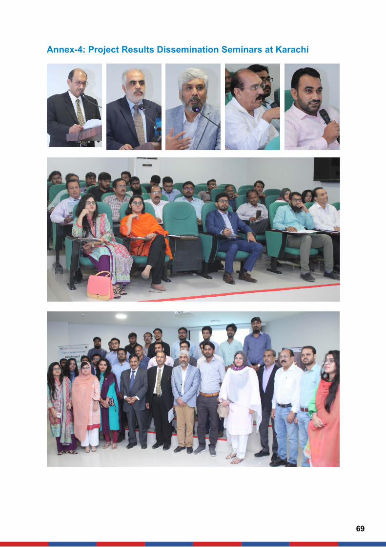
69

Annex-4: Project Results Dissemination Seminars at Karachi

70

Annex-5: Project Results Dissemination Seminars at USPCAS-W, MUET, Jamshoro

Main thrust of Applied Research component of the Water Center is to stimulate an environment that promotes multi-disciplinary research within the broader context of water-development nexus to support evidence-based policy making in the water sector. This is pursued using the framework provided by the six targets of the Sustainable

Development Goal on Water i.e., SDG-6.

About the Author

U.S.-Pakistan Centers for Advanced Studies in WaterMehran University of Engineering and Technology, Jamshoro-76062, Sindh - Pakistan

Contact:

92 22 210 9145 water.muet.edu.pk /USPCASW /USPCASW

Dr. Zubair Ahmed is working as Professor (Environmental Engineering) and Head of department (HoD) (Environmental Engineering) in U.S.- Pakistan Center for Advanced Studies in Water at Mehran University of Engineering and Technology (MUET), Jamshoro. He did his PhD from University of Science and Technology, South Korea. He has been involved in various studies pertinent to operation of MBRs. He has over 20 years of research work experience. During his PhD studies, Dr. Ahmed has utilized sequencing anaerobic/anoxic-aerobic MBRs for removal of nitrogen

and phosphorus. He has been involved in execution and supervision of various research projects including development of polymer based adsorbent for aluminum ion in treated water; removal of gaseous toluene using a pure yeast strain; biodegradation of estrogenic compounds in a pre-anoxic/anaerobic nutrient removing membrane bioreactor and different MBR related studies. His work has been published in a number of top ranked peer reviewed journals. Moreover, Dr. Zubair has conducted various environmental impact assessment and audits in different industrial sectors such as petroleum industry, textile industry, and leather industry.

Treatment and Reuse of Wastewater of Fish Processing Industry

Documents

Transcript of Treatment and Reuse of Wastewater of Fish Processing Industry