Transportation problems - Pearson Schools and FE … · 1 In this chapter you will: † learn the...

1

In this chapter you will:

• learn the terminology used to describe and model transportation problems

• learn about the ‘north-west corner method’

• learn about unbalanced transportation problems

• understand what is meant by a degenerate solution

• learn to fi nd shadow costs

• fi nd improvement indices

• use the stepping-stone method

• formulate a transportation problem as a linear programming problem.

In industry, people are concerned with effi ciency and cost-effectiveness at all stages. In this chapter you will look at the costs due to the transportation of goods – to factories and from factories to warehouses and customers. The problems considered are usually concerned with minimising distribution costs where there are multiple sources and multiple destinations.

1 1

Transportation problemsTransportation problems

CHAPTER 1

2

1.1 You should be familiar with the terminology used in describing and modelling the transportation problem.

In order to solve transportation problems you need to consider:

� The capacity of each of the supply points (or sources) – the quantity of goods that can be produced at each factory or held at each warehouse. This is called the supply or stock.

� The amount required at each of the demand points – the quantity of goods that are needed at each shop or by each customer. This is called the demand (or destination).

� The unit cost of transporting goods from the supply points to the demand points.

Example 1

Three suppliers A, B and C, each produce road grit which has to be delivered to council depots W, X, Y and Z. The stock held at each supplier and the demand from each depot is known. The cost, in pounds, of transporting one lorry load of grit from each supplier to each depot is also known. This information is given in the table.

Depot W

Depot X

Depot Y

Depot Z

Stock (lorry loads)

Supplier A 180 110 130 290 14

Supplier B 190 250 150 280 16

Supplier C 240 270 190 120 20

Demand (lorry loads)

11 15 14 10 50

Use the information in the table to write down:

a the number of lorry loads of grit that each supplier can supply

b the number of lorry loads of grit required at each depot

c the cost of transporting a lorry load of grit from A to W

d the cost of transporting a lorry load of grit from C to Z.

e Which is the cheapest route to use?

f Which is the most expensive route to use?

The unit cost is the cost of transporting one item. If one item costs c pounds to transport from A to X then two items will cost 2c pounds to transport along that route, and n items nc pounds.

This table is often referred to as the cost matrix.

This is the cost of transporting one lorry load from B to Y (in £s).

Notice that the total supply is equal to the total demand. If this is not the case we simply introduce a dummy destination to absorb the excess supply, with transportation costs all zero (see Section 1.3).

Transportation problems

3

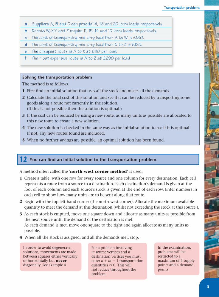
1.2 You can find an initial solution to the transportation problem.

A method often called the ‘north-west corner method’ is used.

1 Create a table, with one row for every source and one column for every destination. Each cell represents a route from a source to a destination. Each destination’s demand is given at the foot of each column and each source’s stock is given at the end of each row. Enter numbers in each cell to show how many units are to be sent along that route.

2 Begin with the top left-hand corner (the north-west corner). Allocate the maximum available quantity to meet the demand at this destination (whilst not exceeding the stock at this source!).

3 As each stock is emptied, move one square down and allocate as many units as possible from the next source until the demand of the destination is met. As each demand is met, move one square to the right and again allocate as many units as possible.

4 When all the stock is assigned, and all the demands met, stop.

a Suppliers A, B and C can provide 14, 16 and 20 lorry loads respectively.b Depots W, X Y and Z require 11, 15, 14 and 10 lorry loads respectively.c The cost of transporting one lorry load from A to W is £180.d The cost of transporting one lorry load from C to Z is £120. e The cheapest route is A to X at £110 per load.f The most expensive route is A to Z at £290 per load

Solving the transportation problem

The method is as follows.

1 First fi nd an initial solution that uses all the stock and meets all the demands.

2 Calculate the total cost of this solution and see if it can be reduced by transporting some goods along a route not currently in the solution. (If this is not possible then the solution is optimal.)

3 If the cost can be reduced by using a new route, as many units as possible are allocated to this new route to create a new solution.

4 The new solution is checked in the same way as the initial solution to see if it is optimal. If not, any new routes found are included.

5 When no further savings are possible, an optimal solution has been found.

In order to avoid degenerate solutions, movements are made between squares either vertically or horizontally but never diagonally. See example 4

For a problem involving m source vertices and n destination vertices you must enter n � m � 1 transportation quantities � 0. This will not reduce throughout the problem.

In the examination, problems will be restricted to a maximum of 4 supply points and 4 demand points.

CHAPTER 1

4

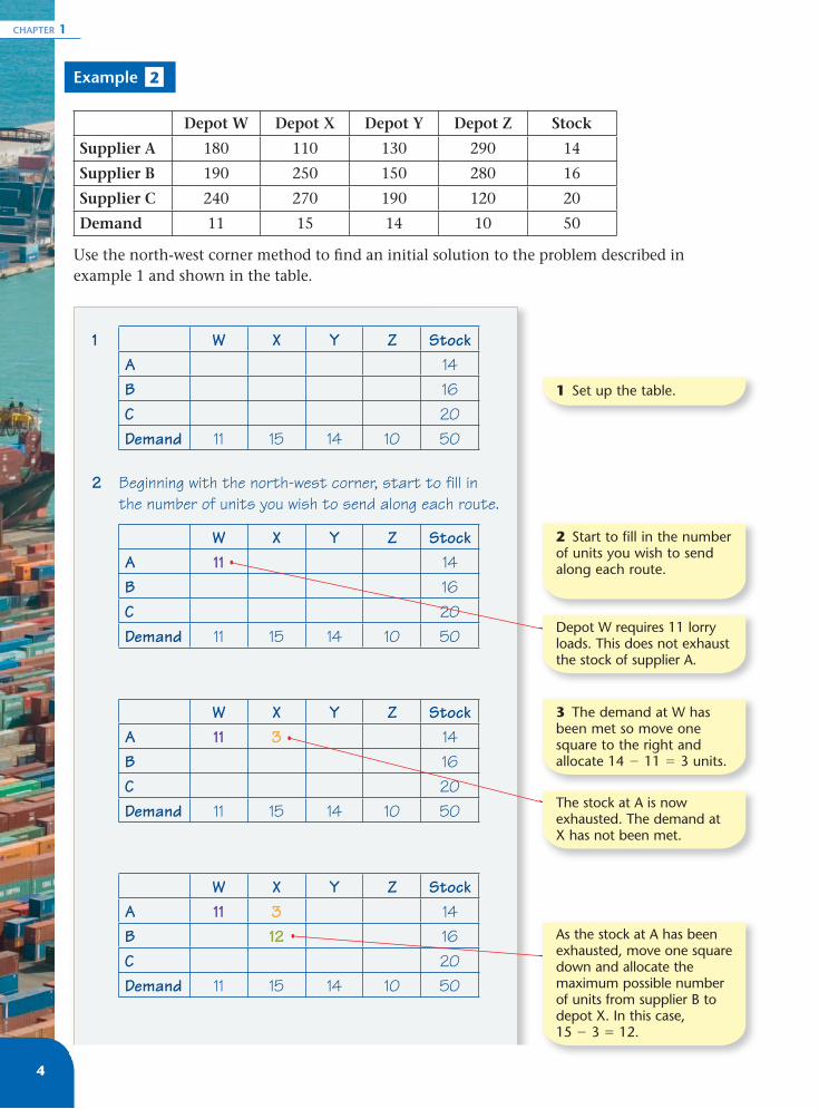
Example 2

Depot W Depot X Depot Y Depot Z Stock

Supplier A 180 110 130 290 14

Supplier B 190 250 150 280 16

Supplier C 240 270 190 120 20

Demand 11 15 14 10 50

Use the north-west corner method to fi nd an initial solution to the problem described in example 1 and shown in the table.

1 W X Y Z StockA 14B 16C 20Demand 11 15 14 10 50

2 Beginning with the north-west corner, start to fill in the number of units you wish to send along each route.

W X Y Z StockA 11 14B 16C 20Demand 11 15 14 10 50

W X Y Z StockA 11 3 14B 16C 20Demand 11 15 14 10 50

W X Y Z StockA 11 3 14B 12 16C 20Demand 11 15 14 10 50

1 Set up the table.

2 Start to fill in the number of units you wish to send along each route.

Depot W requires 11 lorry loads. This does not exhaust the stock of supplier A.

3 The demand at W has been met so move one square to the right and allocate 14 � 11 � 3 units.

The stock at A is now exhausted. The demand at X has not been met.

As the stock at A has been exhausted, move one square down and allocate the maximum possible number of units from supplier B to depot X. In this case, 15 � 3 � 12.


5

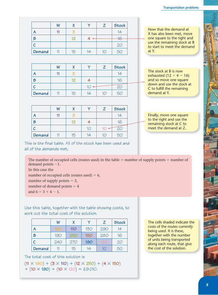
W X Y Z StockA 11 3 14B 12 4 16C 20Demand 11 15 14 10 50

W X Y Z StockA 11 3 14B 12 4 16C 10 20Demand 11 15 14 10 50

W X Y Z StockA 11 3 14B 12 4 16C 10 10 20Demand 11 15 14 10 50

This is the final table. All of the stock has been used and all of the demands met.

Use this table, together with the table showing costs, to work out the total cost of the solution.

W X Y Z StockA 180 110 130 290 14B 190 250 150 280 16C 240 270 190 120 20Demand 11 15 14 10 50

The total cost of this solution is (11 � 180) � (3 � 110) � (12 � 250) � (4 � 150) � (10 � 190) � (10 � 120) � £9 010.

Now that the demand at X has also been met, move one square to the right and use the remaining stock at B to start to meet the demand at Y.

The stock at B is now exhausted (12 � 4 � 16) and so move one square down and use the stock at C to fulfill the remaining demand at Y.

Finally, move one square to the right and use the remaining stock at C to meet the demand at Z.

The number of occupied cells (routes used) in the table � number of supply points � number of demand points �1. In this case the number of occupied cells (routes used) � 6, number of supply points � 3, number of demand points � 4 and 6 � 3 � 4 � 1.

The cells shaded indicate the costs of the routes currently being used. It is these, together with the number of units being transported along each route, that give the cost of the solution.

CHAPTER 1

6

1.3 You can adapt the algorithm to deal with unbalanced transportation problems.

� When the total supply � total demand, we say the problem is unbalanced.

� If the problem is unbalanced we simply add a dummy demand point with a demand chosen so that total supply � total demand, with transportation costs of zero.

Example 3

A B C Supply

X 9 11 10 40

Y 10 8 12 60

Z 12 7 8 50

Demand 50 40 30

Three outlets A, B and C are supplied by three suppliers X, Y and Z. The table shows the cost, in pounds, of transporting each unit, the number of units required at each outlet and the number of units available at each supplier.

a Explain why it is necessary to add a dummy demand point in order to solve this problem.

b Add a dummy demand point and appropriate costs to the table.

c Use the north-west corner method to obtain an initial solution.

a The total supply is 150, but the total demand is 120. A dummy is needed to absorb this excess, so that total supply equals total demand.

b A B C D SupplyX 9 11 10 0 40Y 10 8 12 0 60Z 12 7 8 0 50Demand 50 40 30 30 150

c A B C D SupplyX 40 40Y 10 40 10 60Z 20 30 50Demand 50 40 30 30 150

We add a dummy column, D, where the demand is 30 (the amount by which the supply exceeds the demand), and the transportation costs are zero (since there is no actual transporting done)! The problem is now balanced, the total supply � the total demand.


7

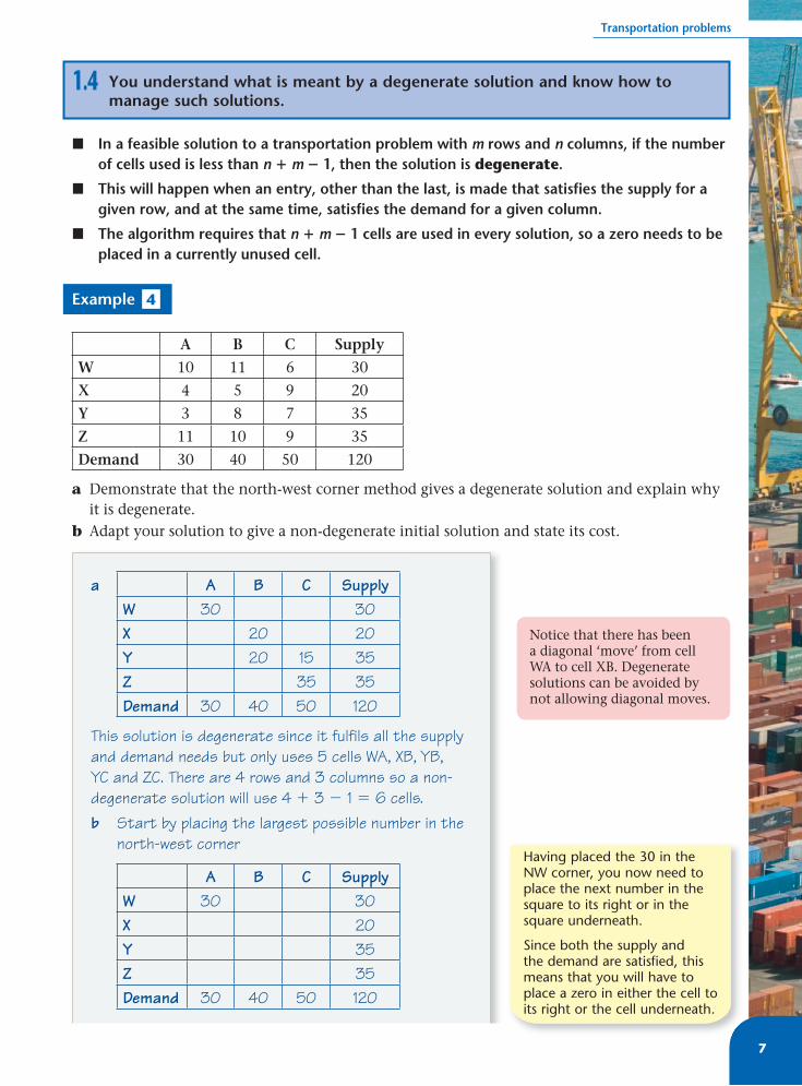
1.4 You understand what is meant by a degenerate solution and know how to manage such solutions.

� In a feasible solution to a transportation problem with m rows and n columns, if the number of cells used is less than n � m � 1, then the solution is degenerate.

� This will happen when an entry, other than the last, is made that satisfi es the supply for a given row, and at the same time, satisfi es the demand for a given column.

� The algorithm requires that n � m � 1 cells are used in every solution, so a zero needs to be placed in a currently unused cell.

Example 4

A B C Supply

W 10 11 6 30

X 4 5 9 20

Y 3 8 7 35

Z 11 10 9 35

Demand 30 40 50 120

a Demonstrate that the north-west corner method gives a degenerate solution and explain why it is degenerate.

b Adapt your solution to give a non-degenerate initial solution and state its cost.

a A B C SupplyW 30 30X 20 20Y 20 15 35Z 35 35Demand 30 40 50 120

This solution is degenerate since it fulfils all the supply and demand needs but only uses 5 cells WA, XB, YB, YC and ZC. There are 4 rows and 3 columns so a non-degenerate solution will use 4 � 3 � 1 � 6 cells.b Start by placing the largest possible number in the

north-west corner

A B C SupplyW 30 30X 20Y 35Z 35Demand 30 40 50 120

Notice that there has been a diagonal ‘move’ from cell WA to cell XB. Degenerate solutions can be avoided by not allowing diagonal moves.

Having placed the 30 in the NW corner, you now need to place the next number in the square to its right or in the square underneath.

Since both the supply and the demand are satisfied, this means that you will have to place a zero in either the cell to its right or the cell underneath.

CHAPTER 1

8

Exercise 1A

Photocopy masters are available for the questions in this exercise.

In Questions 1 to 4, the tables show the unit costs of transporting goods from supply points to demand points. In each case:

a use the north-west corner method to fi nd the initial solution,

b verify that, for each solution, the number of occupied cells � number of supply points � number of demand points � 1.

c determine the cost of each initial solution.

1 P Q R Supply

A 150 213 222 32

B 175 204 218 44

C 188 198 246 34

Demand 28 45 37 110

2 P Q R S Supply

A 27 33 34 41 54

B 31 29 37 30 67

C 40 32 28 35 29

Demand 21 32 51 46 150

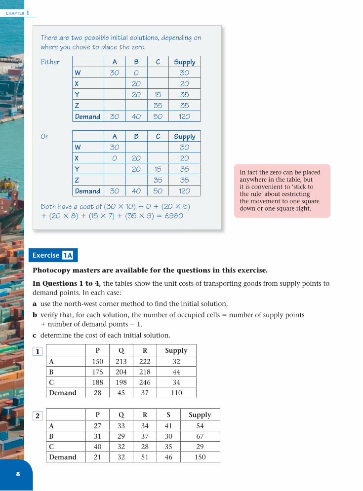
There are two possible initial solutions, depending on where you chose to place the zero.

Either A B C SupplyW 30 0 30X 20 20Y 20 15 35Z 35 35Demand 30 40 50 120

Or A B C SupplyW 30 30X 0 20 20Y 20 15 35Z 35 35Demand 30 40 50 120

Both have a cost of (30 � 10) � 0 � (20 � 5) � (20 � 8) � (15 � 7) � (35 � 9) � £980

In fact the zero can be placed anywhere in the table, but it is convenient to ‘stick to the rule’ about restricting the movement to one square down or one square right.


9

3 P Q R Supply

A 17 24 19 123

B 15 21 25 143

C 19 22 18 84

D 20 27 16 150

Demand 200 100 200 500

4 P Q R S Supply

A 56 86 80 61 134

B 59 76 78 65 203

C 62 70 57 67 176

D 60 68 75 71 187

Demand 175 175 175 175 700

5 A B C D Supply

X 27 33 34 41 60

Y 31 29 37 30 60

Z 40 32 28 35 80

Demand 40 70 50 20

Four sandwich shops A, B, C and D can be supplied with bread from three bakeries, X, Y, and Z. The table shows the cost, in pence, of transporting one tray of bread from each supplier to each shop, the number of trays of bread required by each shop and the number of trays of bread that can be supplied by each bakery.

a Explain why it is necessary to add a dummy demand point in order to solve this problem, and what this dummy point means in practical terms.

b Use the north-west corner method to determine an initial solution to this problem and the cost of this solution.

6 K L M N Supply

A 35 46 62 80 20

B 24 53 73 52 15

C 67 61 50 65 20

D 92 81 41 42 20

Demand 25 10 18 22

A company needs to supply ready-mixed concrete from four depots A, B, C and D to four work sites K, L, M and N. The number of loads that can be supplied from each depot and the number of loads required at each site are shown in the table above, as well as the transportation cost per load from each depot to each work site.

a Explain what is meant by a degenerate solution.

b Demonstrate that the north-west corner method gives a degenerate solution.

c Adapt your solution to give a non-degenerate intial solution.

CHAPTER 1

10

7 L M N Supply

P 3 5 9 22

Q 4 3 7 a

R 6 4 8 11

S 8 2 5 b

Demand 15 17 20

The table shows a balanced transportation problem. The initial solution, given by the north-west corner method, is degenerate.

a Use this information to determine the values of a and b.

b Hence write down the initial, degenerate solution given by the north west-corner method.

1.5 You can find shadow costs.

� Transportation costs are made up of two components, one associated with the source and one with the destination. These costs of using that route, are called shadow costs.


Supplier A 180 110 14

Supplier B 250 150 16

Supplier C 190 120 20

Demand 11 15 14 10 50

In example 2, the cost of £250 in transporting one unit from supplier B to depot X must be dependent on the features � location, toll costs etc, of both B and X.

Using the routes currently in use you can build up equations, showing the cost of transporting one unit, such as

S(A) � D(X) � 110 and S(C) � D(Z) � 120 etc.

where S(A), D(X) are the costs due to supply point A and demand point X and so on, respectively.

You need a value for each of the source components and each of the destination components. You do not have suffi cient equations for a solution (fi ve equations and six unknowns) but relative costs will do.

You are only looking at the costs of the routes used in your current solution.

Finding an improved solution

� To fi nd an improved solution, you need to:

1 use the non-empty cells to fi nd the shadow costs (see Section 1.5)

2 use the shadow costs and the empty cells to fi nd improvement indices (see Section 1.6)

3 use the improvement indices and the stepping stone algorithm to fi nd an improved solution (see Section 1.7).


11

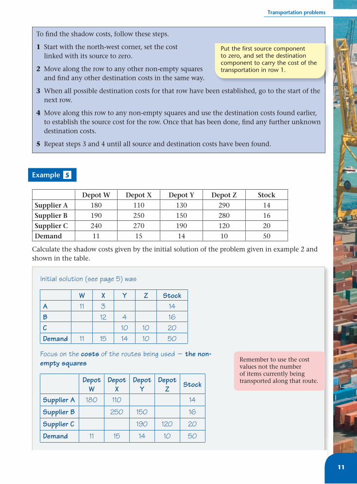
Example 5


Supplier A 180 110 130 290 14

Supplier B 190 250 150 280 16

Supplier C 240 270 190 120 20

Demand 11 15 14 10 50

Calculate the shadow costs given by the initial solution of the problem given in example 2 and shown in the table.

To fi nd the shadow costs, follow these steps.

1 Start with the north-west corner, set the cost linked with its source to zero.

2 Move along the row to any other non-empty squares and fi nd any other destination costs in the same way.

3 When all possible destination costs for that row have been established, go to the start of the next row.

4 Move along this row to any non-empty squares and use the destination costs found earlier, to establish the source cost for the row. Once that has been done, fi nd any further unknown destination costs.

5 Repeat steps 3 and 4 until all source and destination costs have been found.

Put the first source component to zero, and set the destination component to carry the cost of the transportation in row 1.

Initial solution (see page 5) was

W X Y Z StockA 11 3 14B 12 4 16C 10 10 20Demand 11 15 14 10 50

Focus on the costs of the routes being used � the non-empty squares

Depot W

Depot X

Depot Y

Depot Z Stock

Supplier A 180 110 14



Demand 11 15 14 10 50

Remember to use the cost values not the number of items currently being transported along that route.

CHAPTER 1

12

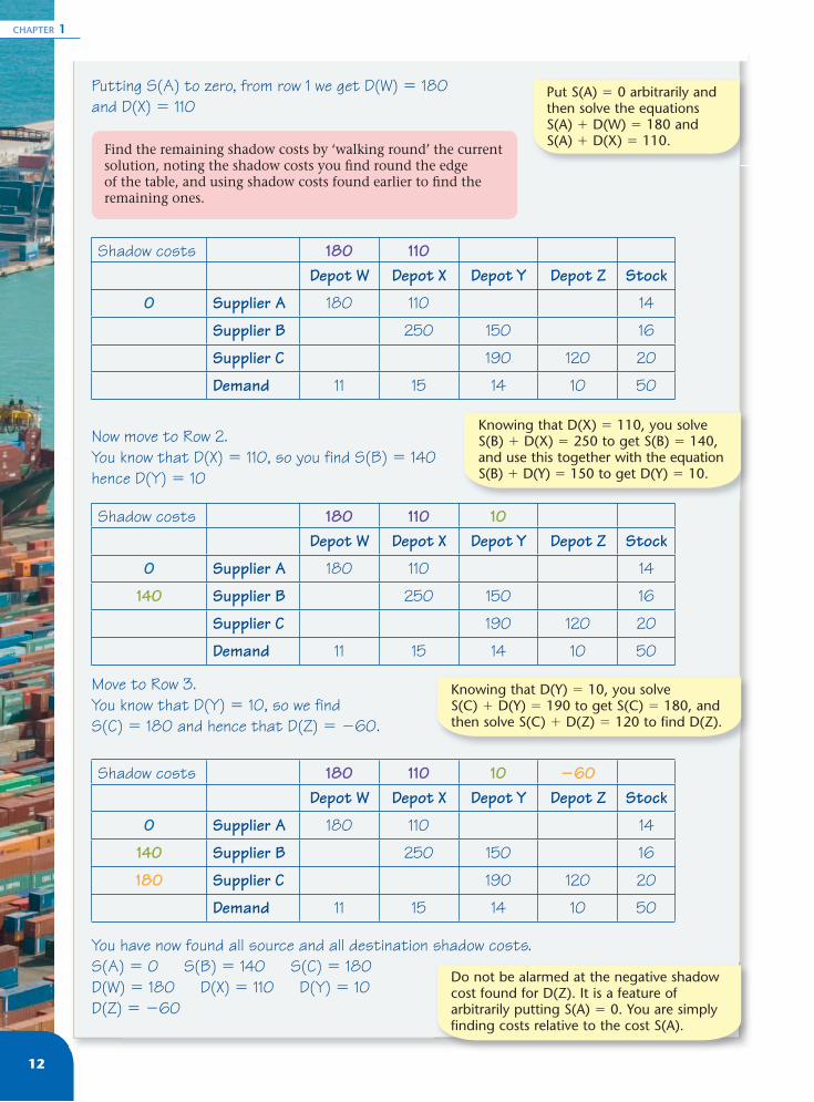
Putting S(A) to zero, from row 1 we get D(W) � 180 and D(X) � 110

Shadow costs 180 110Depot W Depot X Depot Y Depot Z Stock

0 Supplier A 180 110 14



Demand 11 15 14 10 50

Now move to Row 2. You know that D(X) � 110, so you find S(B) � 140 hence D(Y) � 10

Shadow costs 180 110 10Depot W Depot X Depot Y Depot Z Stock

0 Supplier A 180 110 14

140 Supplier B 250 150 16


Demand 11 15 14 10 50

Move to Row 3.You know that D(Y) � 10, so we find S(C) � 180 and hence that D(Z) � �60.

Shadow costs 180 110 10 �60Depot W Depot X Depot Y Depot Z Stock

0 Supplier A 180 110 14

140 Supplier B 250 150 16

180 Supplier C 190 120 20

Demand 11 15 14 10 50

You have now found all source and all destination shadow costs.S(A) � 0 S(B) � 140 S(C) � 180 D(W) � 180 D(X) � 110 D(Y) � 10 D(Z) � �60

Put S(A) � 0 arbitrarily and then solve the equations S(A) � D(W) � 180 and S(A) � D(X) � 110.

Find the remaining shadow costs by ‘walking round’ the current solution, noting the shadow costs you fi nd round the edge of the table, and using shadow costs found earlier to fi nd the remaining ones.

Knowing that D(X) � 110, you solve S(B) � D(X) � 250 to get S(B) � 140, and use this together with the equation S(B) � D(Y) � 150 to get D(Y) � 10.

Knowing that D(Y) � 10, you solve S(C) � D(Y) � 190 to get S(C) � 180, and then solve S(C) � D(Z) � 120 to find D(Z).

Do not be alarmed at the negative shadow cost found for D(Z). It is a feature of arbitrarily putting S(A) � 0. You are simply finding costs relative to the cost S(A).


13

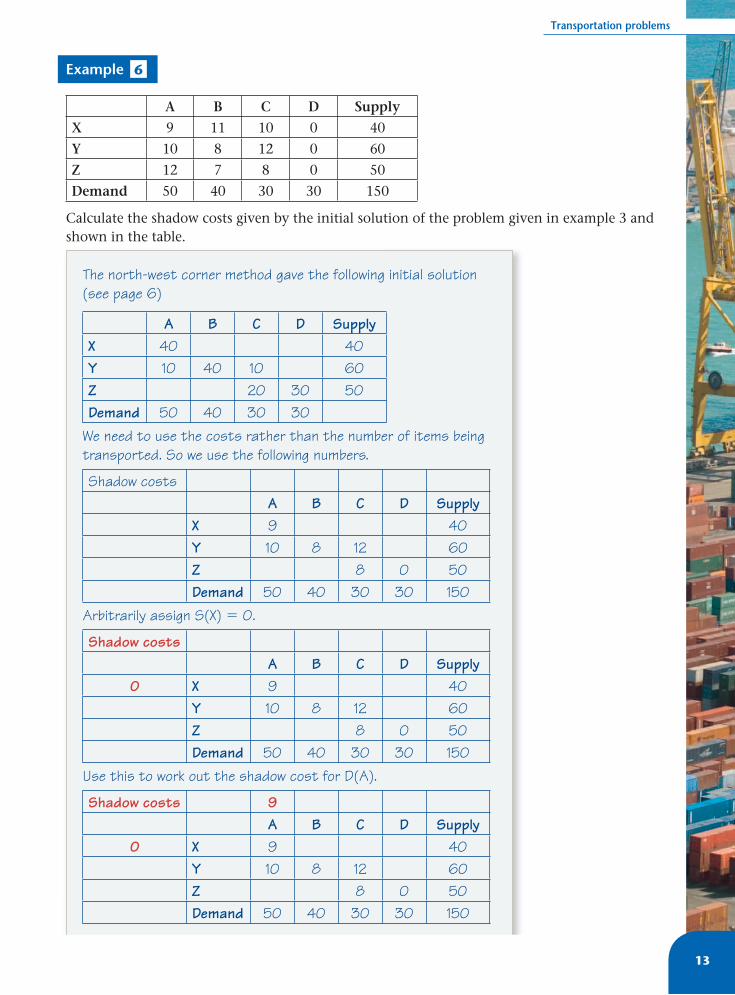
Example 6

A B C D Supply

X 9 11 10 0 40

Y 10 8 12 0 60

Z 12 7 8 0 50

Demand 50 40 30 30 150

Calculate the shadow costs given by the initial solution of the problem given in example 3 and shown in the table.

The north-west corner method gave the following initial solution (see page 6)

A B C D SupplyX 40 40Y 10 40 10 60Z 20 30 50Demand 50 40 30 30

We need to use the costs rather than the number of items being transported. So we use the following numbers.

Shadow costsA B C D Supply

X 9 40Y 10 8 12 60Z 8 0 50Demand 50 40 30 30 150

Arbitrarily assign S(X) � 0.

Shadow costsA B C D Supply

0 X 9 40Y 10 8 12 60Z 8 0 50Demand 50 40 30 30 150

Use this to work out the shadow cost for D(A).

Shadow costs 9A B C D Supply

0 X 9 40Y 10 8 12 60Z 8 0 50Demand 50 40 30 30 150

CHAPTER 1

14

Use this to work out the shadow cost for S(Y).

Shadow costs 9A B C D Supply

0 X 9 401 Y 10 8 12 60

Z 8 0 50Demand 50 40 30 30 150

We use this to work out the shadow costs for D(B) and D(C).

Shadow costs 9 7 11A B C D Supply

0 X 9 401 Y 10 8 12 60

Z 8 0 50Demand 50 40 30 30 150

Use these to work out the shadow cost for S(Z).

Shadow costs 9 7 11A B C D Supply

0 X 9 401 Y 10 8 12 60

�3 Z 8 0 50Demand 50 40 30 30 150

Use this to work out the shadow cost for D(D).

Shadow costs 9 7 11 3A B C D Supply

0 X 9 401 Y 10 8 12 60

�3 Z 8 0 50Demand 50 40 30 30 150

You do not have to show each stage of the table in the examination. Just this fi nal list of shadow costs is suffi cient.


15

1.6 You can find improvement indices and use these to find entering cells.

It may be possible to reduce the cost of the initial solution by introducing a route that is not currently in use. You consider each unused route in turn and calculate the reduction in cost which would be made by sending one unit along that route. This is called the improvement index.

� The improvement index in sending a unit from a source P to a demand point Q is found by subtracting the source cost S(P) and destination cost D(Q) from the stated cost of transporting one unit along that route C(PQ). i.e.

Improvement index for PQ � IPQ� C(PQ) � S(P) � D(Q)

� The route with the most negative improvement index will be introduced into the solution.

� The cell corresponding to the value with the most negative improvement index becomes the entering cell (or entering square or entering route) and the route it replaces is referred to as the exiting cell (or exiting square or exiting route).

� If there are two equal potential entering cells you may choose either. Similarly, if there are two equal exiting cells, you may select either

� If there are no negative improvement indices the solution is optimal.

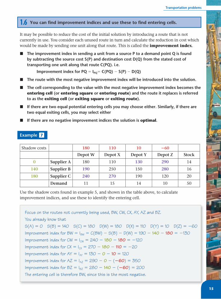
Example 7

Shadow costs 180 110 10 �60


0 Supplier A 180 110 130 290 14

140 Supplier B 190 250 150 280 16

180 Supplier C 240 270 190 120 20

Demand 11 15 14 10 50

Use the shadow costs found in example 5, and shown in the table above, to calculate improvement indices, and use these to identify the entering cell.

Focus on the routes not currently being used, BW, CW, CX, AY, AZ and BZ.You already know that S(A) � 0 S(B) � 140 S(C) � 180 D(W) � 180 D(X) � 110 D(Y) � 10 D(Z) � �60Improvement index for BW � IBW � C(BW) � S(B) � D(W) � 190 � 140 � 180 � �130Improvement index for CW � ICW � 240 � 180 � 180 � �120Improvement index for CX � ICX � 270 � 180 � 110 � �20Improvement index for AY � IAY � 130 � 0 � 10 � 120Improvement index for AZ � IAZ � 290 � 0 � (�60) � 350Improvement index for BZ � IBZ � 280 � 140 � (�60) � 200The entering cell is therefore BW, since this is the most negative.

CHAPTER 1

16

Example 8

X Y Z Supply

A 11 12 17 11

B 13 10 13 15

C 15 18 9 14

Demand 10 15 15

a Use the north-west corner method to fi nd an initial solution to the transportation problem shown in the table.

b Find the shadow costs and improvement indices.

c Hence determine if the solution is optimal.

Exercise 1B

Photocopy masters are available for the questions in this exercise.

Questions 1 to 4Start with the initial, north-west corner, solutions found in questions 1 to 4 of exercise 1A. In each case use the initial solution, and the original cost matrix, shown below, to fi nd a the shadow costs,b the improvement indices c the entering cell, if appropriate.

a X Y Z SupplyA 10 1 11B 14 1 15C 14 14Demand 10 15 15

b Shadow costs 11 12 15X Y Z Supply

0 A 11 12 17 11�2 B 13 10 13 15�6 C 15 18 9 14

Demand 10 15 15

Improvement indices for cells:BX � 13 � 2 � 11 � 4CX � 15 � 6 � 11 � 10CY � 18 � 6 � 12 � 12AZ � 17 � 0 � 15 � 2

c There are no negative improvement indices, so the solution is optimal.


17

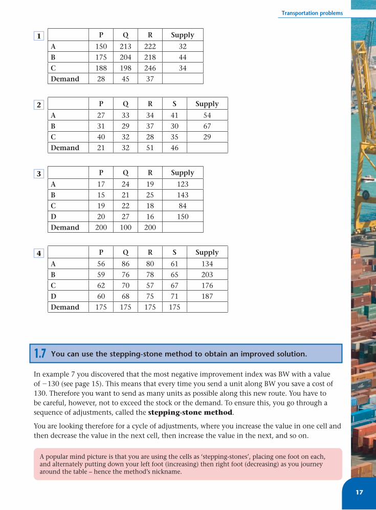
1 P Q R Supply

A 150 213 222 32

B 175 204 218 44

C 188 198 246 34

Demand 28 45 37

2 P Q R S Supply

A 27 33 34 41 54

B 31 29 37 30 67

C 40 32 28 35 29

Demand 21 32 51 46

3 P Q R Supply

A 17 24 19 123

B 15 21 25 143

C 19 22 18 84

D 20 27 16 150

Demand 200 100 200

4 P Q R S Supply

A 56 86 80 61 134

B 59 76 78 65 203

C 62 70 57 67 176

D 60 68 75 71 187

Demand 175 175 175 175

1.7 You can use the stepping-stone method to obtain an improved solution.

In example 7 you discovered that the most negative improvement index was BW with a value of �130 (see page 15). This means that every time you send a unit along BW you save a cost of 130. Therefore you want to send as many units as possible along this new route. You have to be careful, however, not to exceed the stock or the demand. To ensure this, you go through a sequence of adjustments, called the stepping-stone method.

You are looking therefore for a cycle of adjustments, where you increase the value in one cell and then decrease the value in the next cell, then increase the value in the next, and so on.

A popular mind picture is that you are using the cells as ‘stepping-stones’, placing one foot on each, and alternately putting down your left foot (increasing) then right foot (decreasing) as you journey around the table – hence the method’s nickname.

CHAPTER 1

18

Example 9

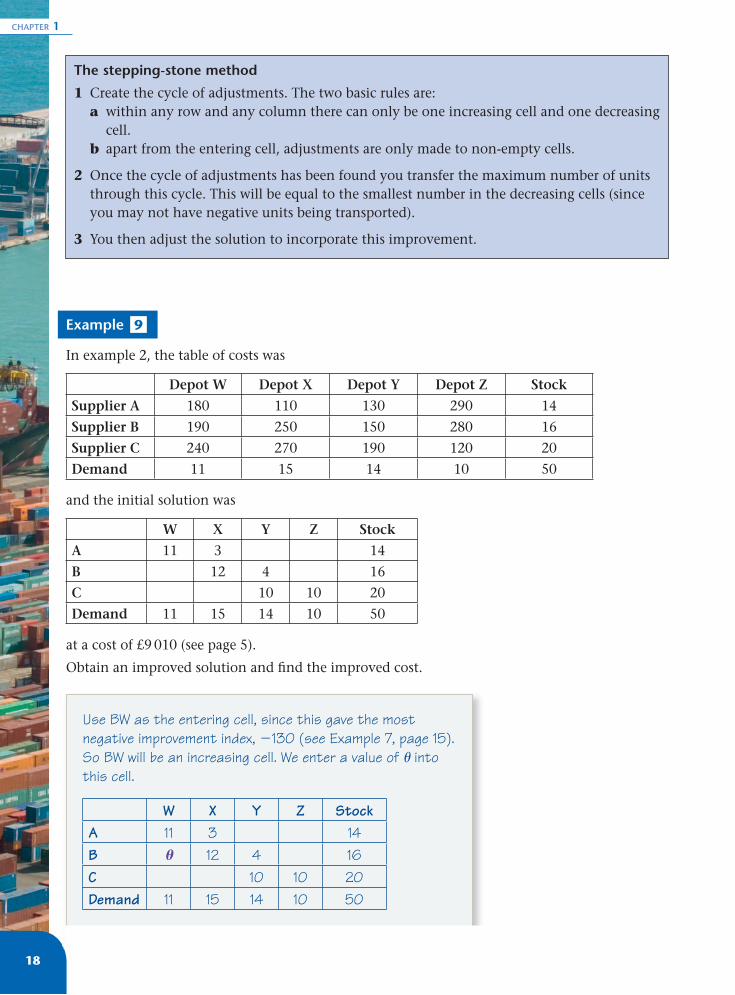
In example 2, the table of costs was


Supplier A 180 110 130 290 14

Supplier B 190 250 150 280 16

Supplier C 240 270 190 120 20

Demand 11 15 14 10 50

and the initial solution was

W X Y Z Stock

A 11 3 14

B 12 4 16

C 10 10 20

Demand 11 15 14 10 50

at a cost of £9 010 (see page 5).

Obtain an improved solution and fi nd the improved cost.

The stepping-stone method

1 Create the cycle of adjustments. The two basic rules are:a within any row and any column there can only be one increasing cell and one decreasing

cell.b apart from the entering cell, adjustments are only made to non-empty cells.

2 Once the cycle of adjustments has been found you transfer the maximum number of units through this cycle. This will be equal to the smallest number in the decreasing cells (since you may not have negative units being transported).

3 You then adjust the solution to incorporate this improvement.

Use BW as the entering cell, since this gave the most negative improvement index, �130 (see Example 7, page 15). So BW will be an increasing cell. We enter a value of � into this cell.

W X Y Z StockA 11 3 14B � 12 4 16C 10 10 20Demand 11 15 14 10 50


19

In order to keep the demand at W correct, you must therefore decrease the entry at AW, so AW will be a decreasing cell.

W X Y Z StockA 11 � � 3 14B � 12 4 16C 10 10 20Demand 11 15 14 10 50

In order to keep the stock at A correct, you must therefore increase the entry at AX, so AX will be an increasing cell.

W X Y Z StockA 11 � � 3 � � 14B � 12 4 16C 10 10 20Demand 11 15 14 10 50

In order to keep the demand at X correct, you must therefore decrease the entry at BX, so BX will be a decreasing cell.

W X Y Z StockA 11 � � 3 � � 14B � 12 � � 4 16C 10 10 20Demand 11 15 14 10 50

Now choose a value for �, the greatest value you can, without introducing negative entries into the table. Look at the decreasing cells and see that the greatest value of � is 11 (since 11 � 11 � 0).

Replace � by 11 in the table:

W X Y Z StockA 11 � 11 3 � 11 14B 11 12 � 11 4 16C 10 10 20Demand 11 15 14 10 50

This is as far as you can go with adjustments since the top two rows both have an increasing and decreasing cell.

CHAPTER 1

20

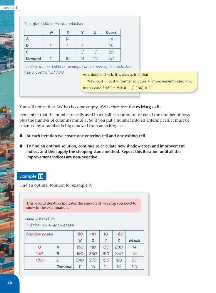
You will notice that AW has become empty. AW is therefore the exiting cell.

Remember that the number of cells used in a feasible solution must equal the number of rows plus the number of columns minus 1. So if you put a number into an entering cell, it must be balanced by a number being removed from an exiting cell.

� At each iteration we create one entering cell and one exiting cell.

� To fi nd an optimal solution, continue to calculate new shadow costs and improvement indices and then apply the stepping-stone method. Repeat this iteration until all the improvement indices are non-negative.

Example 10

Find an optimal solution for example 9.

This gives the improved solution:

W X Y Z StockA 14 14B 11 1 4 16C 10 10 20Demand 11 15 14 10 50

Looking at the table of transportation costs, this solution has a cost of £7 580

As a double check, it is always true that

New cost � cost of former solution � improvement index � �.

In this case 7 580 � 9 010 � (�130) � 11

Second iterationFind the new shadow costs:

Shadow costs 50 110 10 �60W X Y Z Stock

0 A 180 110 130 290 14140 B 190 250 150 280 16180 C 240 270 190 120 20

Demand 11 15 14 10 50

This second iteration indicates the amount of working you need to show in the examination.


21

Finding the new improvement indices for the non-used cells:AW � 180 � 0 � 50 � 130CW � 240 � 180 � 50 � 10CX � 270 � 180 � 110 � �20AY � 130 � 0 � 10 � 120AZ � 290 � 0 � 60 � 350BZ � 280 � 140 � 60 � 200

So the new entering cell is CX, since this has the most negative improvement index.

Applying the stepping-stone method gives

W X Y Z StockA 14 14B 11 1 � � 4 � � 16C � 10 � � 10 20Demand 11 15 14 10 50

Looking at cells BX and CY we see that the greatest value for � is 1

The new exiting cell will be BX, � � 1 and we get

W X Y Z StockA 14 14B 11 5 16C 1 9 10 20Demand 11 15 14 10 50

The new cost is £7 560

Third iterationNew shadow costs

Shadow costs 70 110 30 �40W X Y Z Stock

0 A 180 110 130 290 14120 B 190 250 150 280 16160 C 240 270 190 120 20

Demand 11 15 14 10 50

Checking, 7 580 � (�20) � 1 � 7560

CHAPTER 1

22

Some stepping-stone routes are not rectangles and some � values are not immediately apparent.

Example 11

Supermarket X Supermarket Y Supermarket Z Stock

Warehouse A 24 22 28 13

Warehouse B 26 26 14 11

Warehouse C 20 22 20 12

Demand 10 13 13

The table shows the unit cost, in pounds, of transporting goods from each of three warehouses, A, B and C to each of three supermarkets X, Y and Z. It also shows the stock at each warehouse and the demand at each supermarket.

Solve the transportation problem shown in the table. Use the north-west corner method to obtain an initial solution. You must state your shadow costs, improvement indices, stepping-stone routes, � values, entering cells and exiting cells. You must state the initial cost and the improved cost after each iteration.

New improvement indices for the non-used cells:

AW � 180 � 0 � 70 � 110CW � 240 � 160 � 70 � 10BX � 250 � 120 � 110 � 20AY � 130 � 0 � 30 � 100AZ � 290 � 0 � 40 � 330BZ � 280 � 120 � 40 � 200

There are no negative improvement indices so this solution is optimal.

The solution is 110 units A to X190 units B to W150 units B to Y270 units C to X190 units C to Y120 units C to Z

At this point, if there is an improvement index of 0, this would indicate that there is an alternative optimal solution. To fi nd it, simply use the cell with the zero improvement index as the entering cell. (See question 2 in Mixed Exercise 1E.)

Check the problem is balanced, Supply � Demand � 36, so we do not need to add a dummy.The north-west corner method gives the following initial solution

X Y Z StockA 10 3 13B 10 1 11C 12 12Demand 10 13 13


23

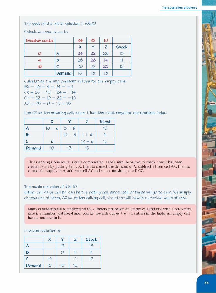
The cost of the initial solution is £820

Calculate shadow costs

Shadow costs 24 22 10X Y Z Stock

0 A 24 22 28 134 B 26 26 14 1110 C 20 22 20 12

Demand 10 13 13

Calculating the improvement indices for the empty cells:BX � 26 � 4 � 24 � �2CX � 20 � 10 � 24 � �14CY � 22 � 10 � 22 � �10AZ � 28 � 0 � 10 � 18

Use CX as the entering cell, since it has the most negative improvement index.

X Y Z StockA 10 � � 3 � � 13B 10 � � 1 � � 11C � 12 � � 12Demand 10 13 13

The maximum value of � is 10Either cell AX or cell BY can be the exiting cell, since both of these will go to zero. We simply choose one of them, AX to be the exiting cell, the other will have a numerical value of zero.

Improved solution is

X Y Z StockA 13 13B 0 11 11C 10 2 12Demand 10 13 13

This stepping stone route is quite complicated. Take a minute or two to check how it has been created. Start by putting � in CX, then to correct the demand of X, subtract � from cell AX, then to correct the supply in A, add � to cell AY and so on, fi nishing at cell CZ.

Many candidates fail to understand the difference between an empty cell and one with a zero entry. Zero is a number, just like 4 and ‘counts’ towards our m � n � 1 entries in the table. An empty cell has no number in it.

CHAPTER 1

24

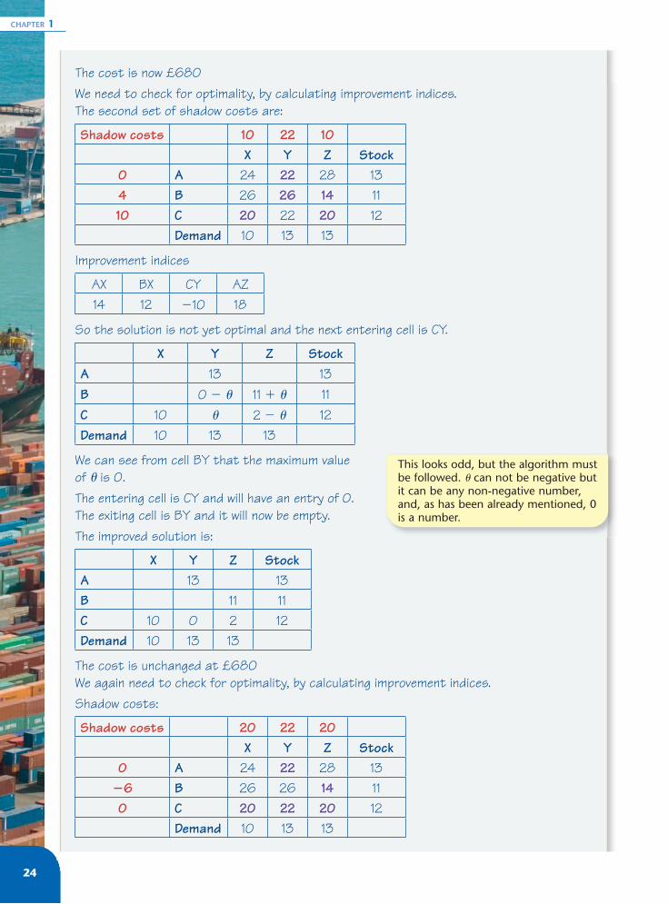
The cost is now £680We need to check for optimality, by calculating improvement indices.The second set of shadow costs are:


0 A 24 22 28 134 B 26 26 14 1110 C 20 22 20 12

Demand 10 13 13

Improvement indices

AX BX CY AZ14 12 �10 18

So the solution is not yet optimal and the next entering cell is CY.

X Y Z StockA 13 13B 0 � � 11 � � 11C 10 � 2 � � 12Demand 10 13 13

We can see from cell BY that the maximum value of � is 0.The entering cell is CY and will have an entry of 0.The exiting cell is BY and it will now be empty.The improved solution is:

X Y Z StockA 13 13B 11 11C 10 0 2 12Demand 10 13 13

The cost is unchanged at £680We again need to check for optimality, by calculating improvement indices.Shadow costs:


0 A 24 22 28 13�6 B 26 26 14 110 C 20 22 20 12

Demand 10 13 13

This looks odd, but the algorithm must be followed. � can not be negative but it can be any non-negative number, and, as has been already mentioned, 0 is a number.


25

Exercise 1C

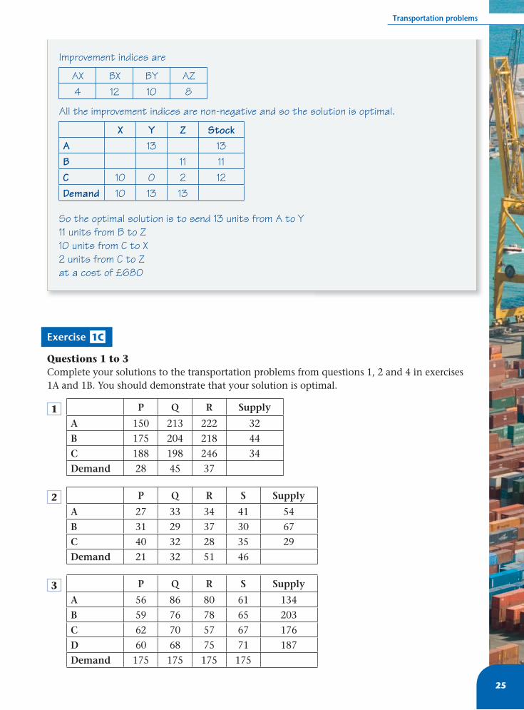
Questions 1 to 3Complete your solutions to the transportation problems from questions 1, 2 and 4 in exercises 1A and 1B. You should demonstrate that your solution is optimal.

1 P Q R Supply

A 150 213 222 32

B 175 204 218 44

C 188 198 246 34

Demand 28 45 37

2 P Q R S Supply

A 27 33 34 41 54

B 31 29 37 30 67

C 40 32 28 35 29

Demand 21 32 51 46

3 P Q R S Supply

A 56 86 80 61 134

B 59 76 78 65 203

C 62 70 57 67 176

D 60 68 75 71 187

Demand 175 175 175 175

Improvement indices are

AX BX BY AZ4 12 10 8

All the improvement indices are non-negative and so the solution is optimal.

X Y Z StockA 13 13B 11 11C 10 0 2 12Demand 10 13 13

So the optimal solution is to send 13 units from A to Y11 units from B to Z10 units from C to X2 units from C to Zat a cost of £680

CHAPTER 1

26

4 P Q Stock

A 2 6 3

B 2 7 5

C 6 9 2

Demand 6 4

Solve the transportation problem shown in the table. Use the north-west corner method to obtain an initial solution. You must state your shadow costs, improvement indices, stepping-stone routes, � values, entering cells and exiting cells. You must state the initial cost and the improved cost after each iteration.

1.8 You can formulate a transportation problem as a linear programming problem.

Consider our fi rst example


Supplier A 180 110 130 290 14

Supplier B 190 250 150 280 16

Supplier C 240 270 190 120 20

Demand 11 15 14 10 50

Let x11 (the entry in the 1st row, 1st column) be the number of units transported from A to W, and x24 (the entry in the 2nd row and 4th column) be the number of units transported from B to Z, and so on, then you have the following solution.


Supplier A x11 x12 x13 x14 14

Supplier B x21 x22 x23 x24 16

Supplier C x31 x32 x33 x34 20

Demand 11 15 14 10 50

The objective is to minimise the total cost, which will be calculated by fi nding the sum of the product of number of units transported along each route and the cost of using that route.

The solution to question 3 requires a number of iterations, plus the optimality check – you will certainly get lots of practise in implementing the algorithms!

x11, x23, x34 and so on are called the decision variables.

In this case a lot of these entries will be empty � there will be only 3 � 4 � 1 � 6 non-empty cells, and all the rest will be blank. However, since you do not yet know which will be empty you allow for any of them to be non-empty as you formulate the problem.

The table shows the unit cost, in pounds, of transporting goods from each of three warehouses A, B and C to each of two supermarkets P and Q. It also shows the stock at each warehouse and the demand at each supermarket.

In book D1 you met linear programming problems in two variables. In chapter 4 of this book you will study linear programming problems in more than two variables.


27

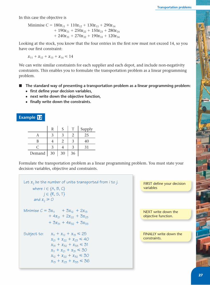
In this case the objective is

Minimise C � 180x11 � 110x12 � 130x13 � 290x14 � 190x21 � 250x22 � 150x23 � 280x24 � 240x31 � 270x32 � 190x33 � 120x34

Looking at the stock, you know that the four entries in the fi rst row must not exceed 14, so you have our fi rst constraint:

x11 � x12 � x13 � x14 14

We can write similar constraints for each supplier and each depot, and include non-negativity constraints. This enables you to formulate the transportation problem as a linear programming problem.

� The standard way of presenting a transportation problem as a linear programming problem:• fi rst defi ne your decision variables,• next write down the objective function,• fi nally write down the constraints.

Example 12

R S T Supply

A 3 3 2 25

B 4 2 3 40

C 3 4 3 31

Demand 30 30 36

Formulate the transportation problem as a linear programming problem. You must state your decision variables, objective and constraints.

Let xij be the number of units transported from i to j.where i ∈ {A, B, C}

j ∈ {R, S, T }and xij � 0

Minimise C � 3x11 � 3x12 � 2x13 � 4x21 � 2x22 � 3x23 � 3x31 � 4x32 � 3x33

Subject to: x11 � x12 � x13 25x21 � x22 � x23 40x31 � x32 � x33 31x11 � x21 � x31 30x12 � x22 � x32 30x13 � x23 � x33 36

FIRST define your decision variables

NEXT write down the objective function.

FINALLY write down the constraints.

CHAPTER 1

28

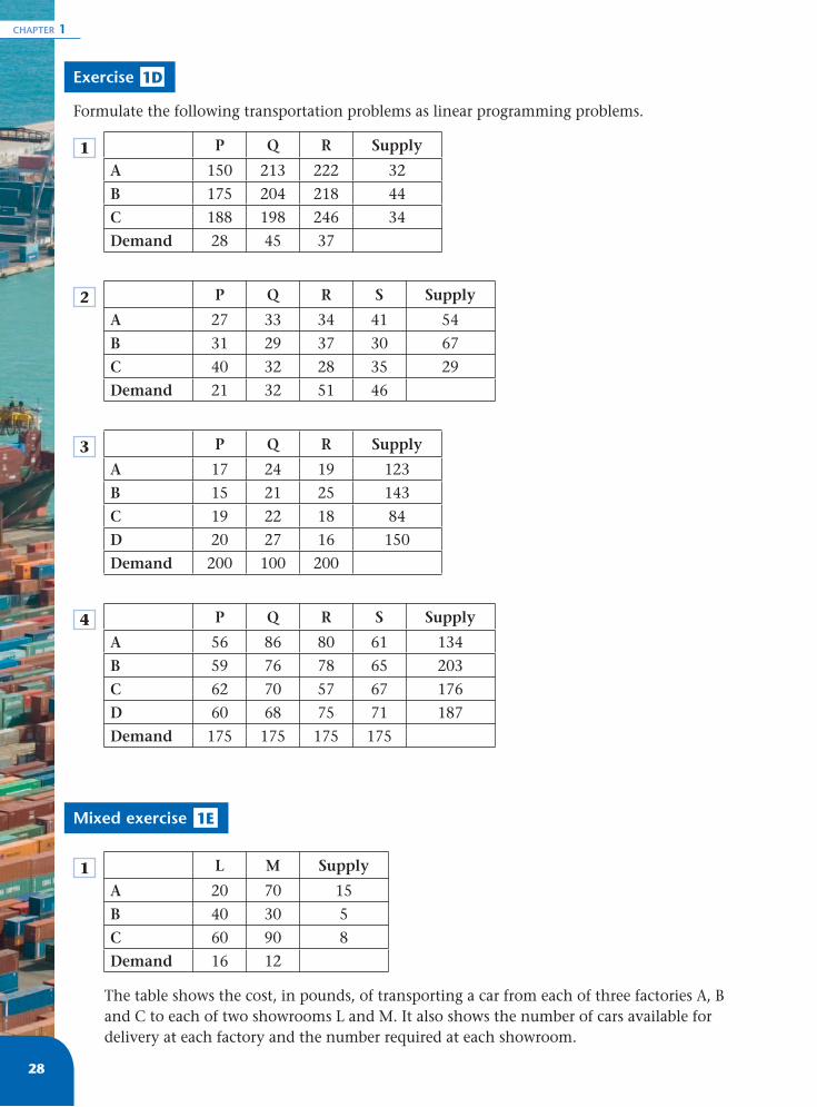
Exercise 1D

Formulate the following transportation problems as linear programming problems.

1 P Q R Supply

A 150 213 222 32

B 175 204 218 44

C 188 198 246 34

Demand 28 45 37

2 P Q R S Supply

A 27 33 34 41 54

B 31 29 37 30 67

C 40 32 28 35 29

Demand 21 32 51 46

3 P Q R Supply

A 17 24 19 123

B 15 21 25 143

C 19 22 18 84

D 20 27 16 150

Demand 200 100 200

4 P Q R S Supply

A 56 86 80 61 134

B 59 76 78 65 203

C 62 70 57 67 176

D 60 68 75 71 187

Demand 175 175 175 175

Mixed exercise 1E

1 L M Supply

A 20 70 15

B 40 30 5

C 60 90 8

Demand 16 12

The table shows the cost, in pounds, of transporting a car from each of three factories A, B and C to each of two showrooms L and M. It also shows the number of cars available for delivery at each factory and the number required at each showroom.


29

a Use the north-west corner method to fi nd an initial solution.

b Solve the transportation problem, stating shadow costs, improvement indices, entering cells, stepping-stone routes, � values and exiting cells.

c Demonstrate that your solution is optimal and fi nd the cost of your optimal solution.

d Formulate this problem as a linear programming problem, making your decision variables, objective function and constraints clear.

e Verify that your optimal solution lies in the feasible region of the linear programming problem.

2 P Q R Supply

F 23 21 22 15

G 21 23 24 35

H 22 21 23 10

Demand 10 30 20

The table shows the cost of transporting one unit of stock from each of three supply points F, G and H to each of three sales points P, Q and R. It also shows the stock held at each supply point and the amount required at each sales point.

a Use the north-west corner method to obtain an initial solution.

b Taking the most negative improvement index to indicate the entering square, perform two complete iterations of the stepping-stone method. You must state your shadow costs, improvement indices, stepping-stone routes and exiting cells.

c Explain how you can tell that your current solution is optimal.

d State the cost of your optimal solution.

e Taking the zero improvement index to indicate the entering square, perform one futher iteration to obtain a second optimal solution.

3 X Y Z Supply

J 8 5 7 30

K 5 5 9 40

L 7 2 10 50

M 6 3 15 50

Demand 25 45 100

The transportation problem represented by the table above is to be solved.

A possible north-west corner solution is

X Y Z Supply

J 25 5 30

K 40 40

L 0 50 50

M 50 50

Demand 25 45 100

CHAPTER 1

30

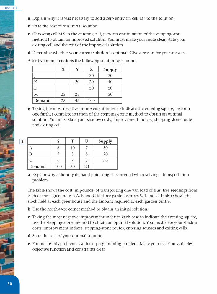
a Explain why it is was necessary to add a zero entry (in cell LY) to the solution.

b State the cost of this initial solution.

c Choosing cell MX as the entering cell, perform one iteration of the stepping-stone method to obtain an improved solution. You must make your route clear, state your exiting cell and the cost of the improved solution.

d Determine whether your current solution is optimal. Give a reason for your answer.

After two more iterations the following solution was found.

X Y Z Supply

J 30 30

K 20 20 40

L 50 50

M 25 25 50

Demand 25 45 100

e Taking the most negative improvement index to indicate the entering square, perform one further complete iteration of the stepping-stone method to obtain an optimal solution. You must state your shadow costs, improvement indices, stepping-stone route and exiting cell.

4 S T U Supply

A 6 10 7 50

B 7 5 8 70

C 6 7 7 50

Demand 100 30 20

a Explain why a dummy demand point might be needed when solving a transportation problem.

The table shows the cost, in pounds, of transporting one van load of fruit tree seedlings from each of three greenhouses A, B and C to three garden centres S, T and U. It also shows the stock held at each greenhouse and the amount required at each garden centre.

b Use the north-west corner method to obtain an initial solution.

c Taking the most negative improvement index in each case to indicate the entering square, use the stepping-stone method to obtain an optimal solution. You must state your shadow costs, improvement indices, stepping-stone routes, entering squares and exiting cells.

d State the cost of your optimal solution.

e Formulate this problem as a linear programming problem. Make your decision variables, objective function and constraints clear.


31

Summary of key points1 In solving transportation problems, you need to know

• the supply or stock• the demand• the unit cost of transporting goods.

2 When total supply � total demand, the problem is unbalanced.

3 A dummy destination is needed if total supply does not equal total demand. Transport costs to this dummy destination are zero.

4 To solve the transportation problem, the north-west corner method is used.

5 The north-west corner method:� Create a table, with one row for every source and one column for every destination.

Each destination’s demand is given at the foot of each column and each source’s stock is given at the end of each row. Enter numbers in each cell to show how many units are to be sent along that route.

� Begin with the top left-hand corner. Allocate the maximum available quantity to meet the demand at this destination (but do not exceed the stock at this source).

� As each stock is emptied, move one square down and allocate as many units as possible from the next source until the demand of the destination is met.

� As each demand is met, move one square to the right and again allocate as many units as possible.

� Stop when all the stock is assigned and all the demands are met.

6 In a feasible solution to a transportation problem with m rows and n columns, if the number of cells used is less than n � m � 1 then the solution is degenerate.

7 The algorithm requires n � m � 1 cells to be used in every solution, so a zero must be placed in an unused cell in a degenerate solution.

8 To fi nd an improved solution, you need to:� use the non-empty cells to fi nd the shadow costs� use the shadow costs and the empty cells to fi nd improvement indices� use the improvement indices and the stepping-stones method to fi nd an improved

solution.

9 Transportation costs are made up of two components, one associated with the source and one with the destination. The costs of using a route are called shadow costs. (See example 5 for how to work out shadow costs.)

10 The improvement index of a route is the reduction in cost which would be made by sending one unit along that route. Improvement index for route PQ � IPQ � C(PQ) � S(P) � D(Q) (see example 7).

11 The stepping-stone method is used to fi nd an improved solution (see example 9).

Transportation problems - Pearson Schools and FE … · 1 In this chapter you will: † learn the...

Documents

Transcript of Transportation problems - Pearson Schools and FE … · 1 In this chapter you will: † learn the...