Transportation Problems-Optimality Check

Dr. Naval Karrir

1

2

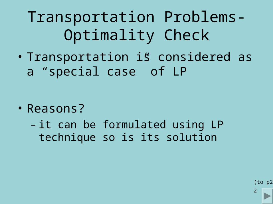
Transportation Problems- Optimality Check

• Transportation is considered as a “special case” of LP

• Reasons?– it can be formulated using LP technique so is

its solution

(to p2)

3

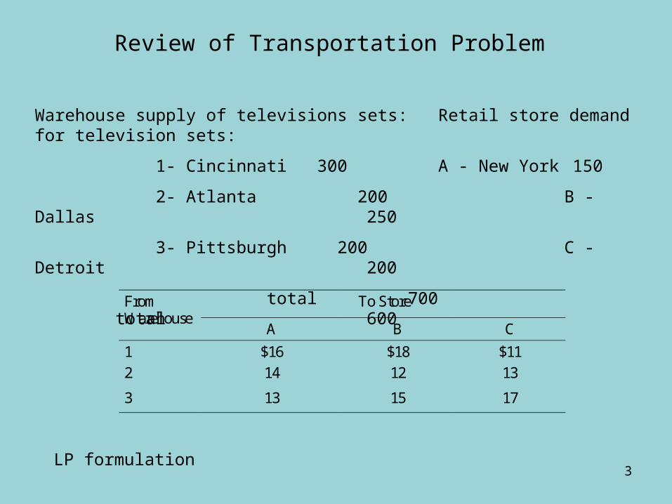
Review of Transportation Problem

Warehouse supply of televisions sets: Retail store demand for television sets:

1- Cincinnati 300 A - New York 150

2- Atlanta 200 B - Dallas 250

3- Pittsburgh 200 C - Detroit 200

total 700 total 600

To StoreFromWarehouse

A B C

1 $16 $18 $11

2 14 12 13

3 13 15 17

LP formulation

4

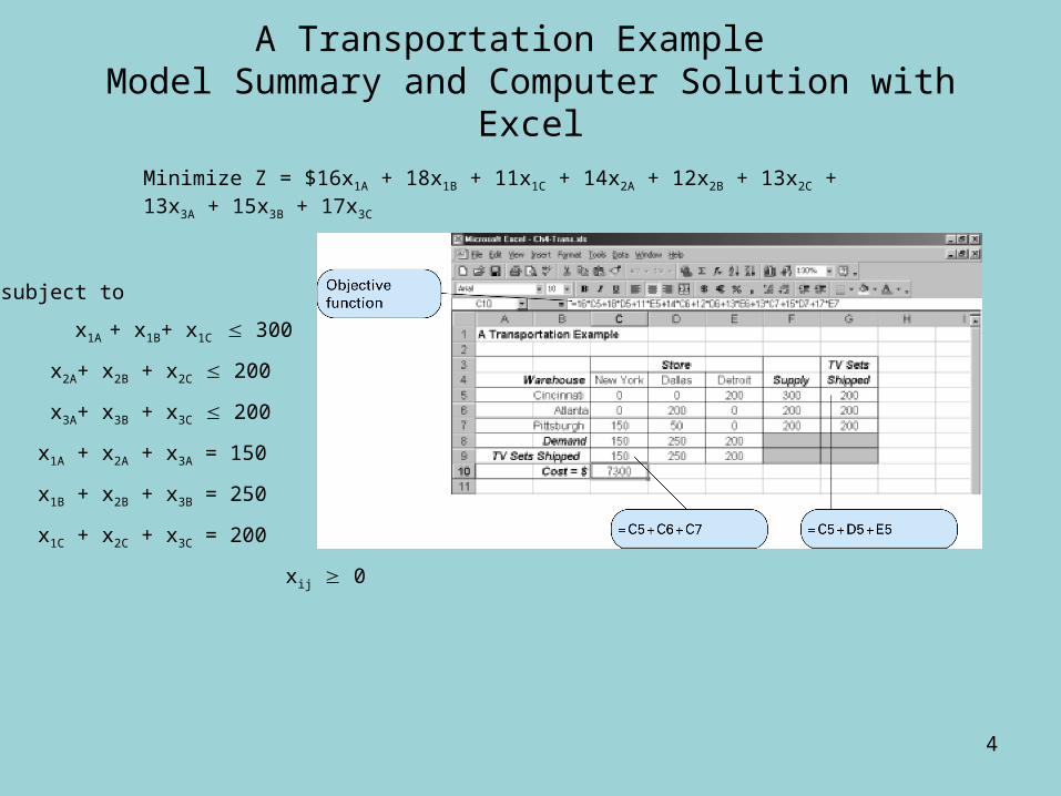
A Transportation Example Model Summary and Computer Solution with Excel

Minimize Z = $16x1A + 18x1B + 11x1C + 14x2A + 12x2B + 13x2C + 13x3A + 15x3B + 17x3C

subject to

x1A + x1B+ x1C 300

x2A+ x2B + x2C 200

x3A+ x3B + x3C 200

x1A + x2A + x3A = 150

x1B + x2B + x3B = 250

x1C + x2C + x3C = 200

xij 0

5

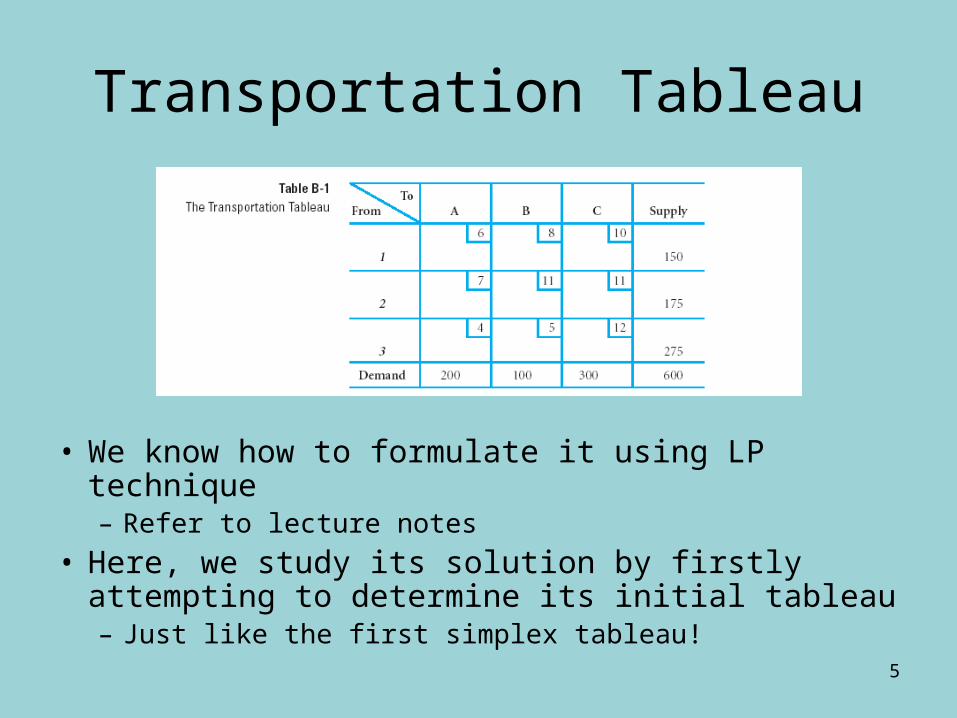
Transportation Tableau

• We know how to formulate it using LP technique– Refer to lecture notes

• Here, we study its solution by firstly attempting to determine its initial tableau– Just like the first simplex tableau!

6

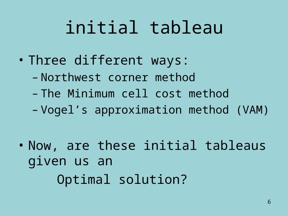
initial tableau

• Three different ways:– Northwest corner method– The Minimum cell cost method– Vogel’s approximation method (VAM)

• Now, are these initial tableaus given us an

Optimal solution?

7

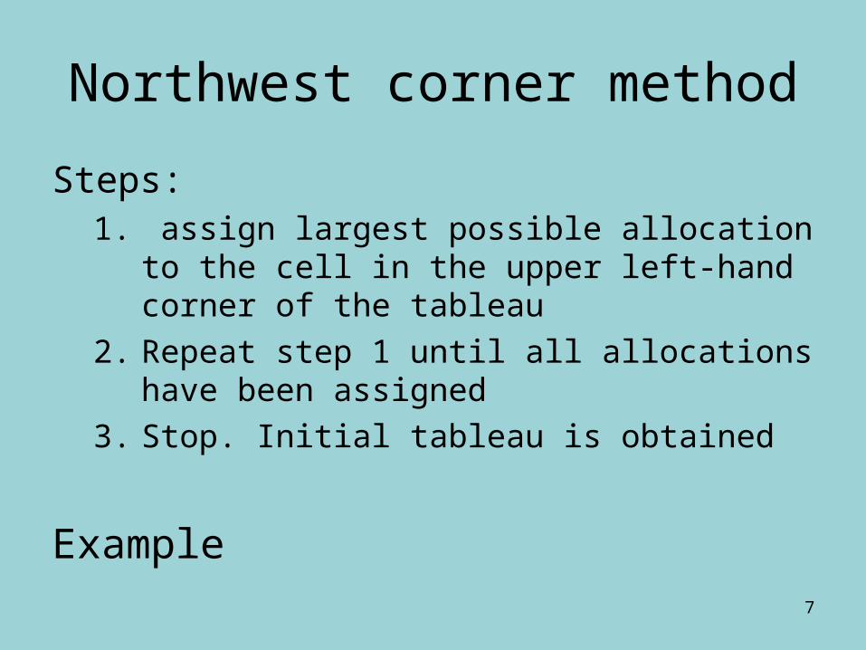
Northwest corner method

Steps:1. assign largest possible allocation to the cell

in the upper left-hand corner of the tableau

2. Repeat step 1 until all allocations have been assigned

3. Stop. Initial tableau is obtained

Example

8

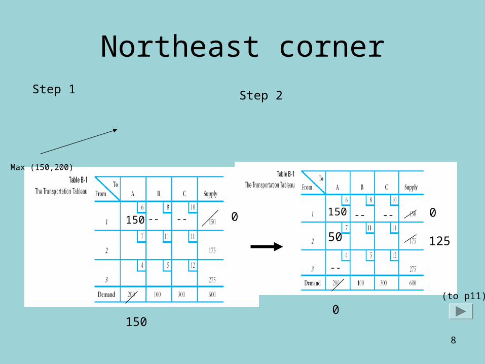
Northeast corner

150

Step 1

Max (150,200)

Step 2

150

50

-- -- 0

150

--

--

-- 0

0

125

(to p11)

9

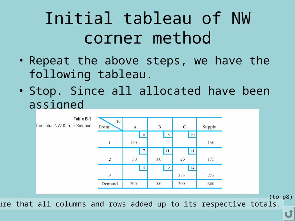
Initial tableau of NW corner method

• Repeat the above steps, we have the following tableau.

• Stop. Since all allocated have been assigned

Ensure that all columns and rows added up to its respective totals.(to p8)

10

The Minimum cell cost method

Here, we use the following steps:

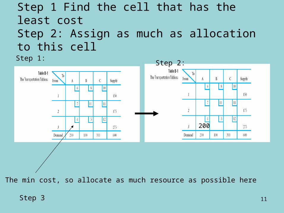
Steps:Step 1 Find the cell that has the least cost

Step 2: Assign as much as allocation to this cell

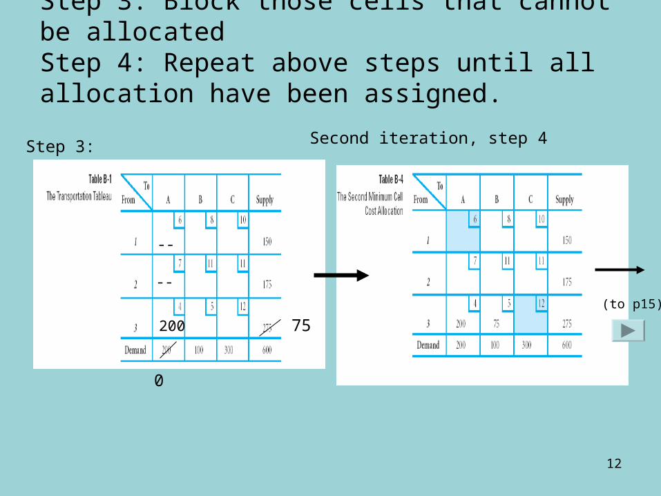
Step 3: Block those cells that cannot be allocated

Step 4: Repeat above steps until all allocation have been assigned.

Example:

11

Step 1 Find the cell that has the least costStep 2: Assign as much as allocation to this cell

Step 1:

The min cost, so allocate as much resource as possible here

200

Step 3

Step 2:

12

Step 3: Block those cells that cannot be allocatedStep 4: Repeat above steps until all allocation have been assigned.

Step 3:

200

--

--

0

75

Second iteration, step 4

(to p15)

13

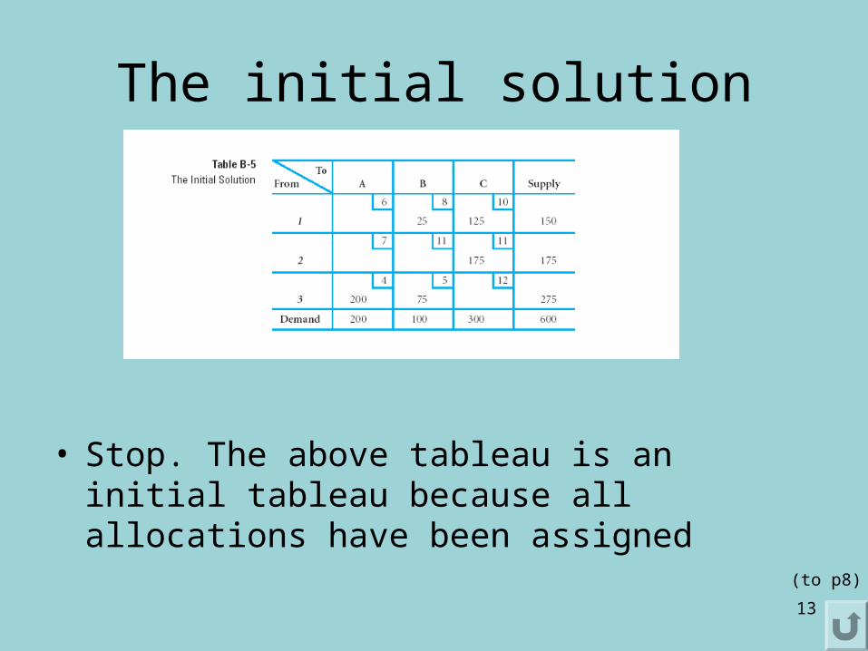
The initial solution

• Stop. The above tableau is an initial tableau because all allocations have been assigned

(to p8)

14

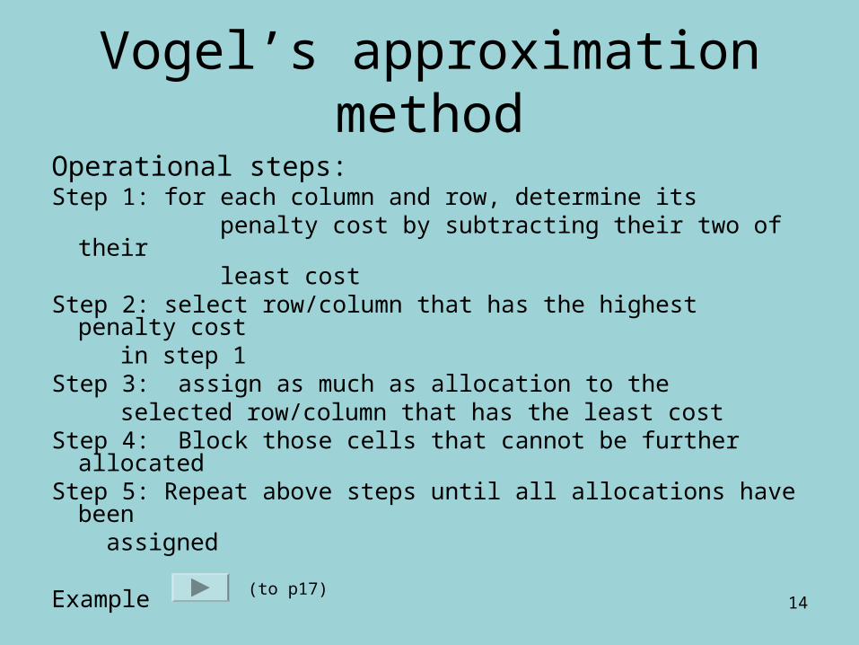
Vogel’s approximation method

Operational steps:Step 1: for each column and row, determine its penalty cost by subtracting their two of their

least cost Step 2: select row/column that has the highest penalty cost

in step 1Step 3: assign as much as allocation to the

selected row/column that has the least costStep 4: Block those cells that cannot be further allocatedStep 5: Repeat above steps until all allocations have been

assigned

Example(to p17)

15

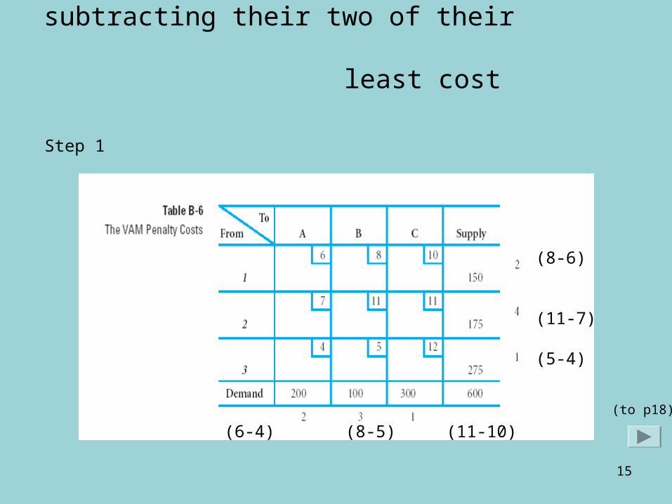
subtracting their two of their least cost

Step 1

(8-6)

(11-7)

(5-4)

(6-4) (8-5) (11-10)(to p18)

16

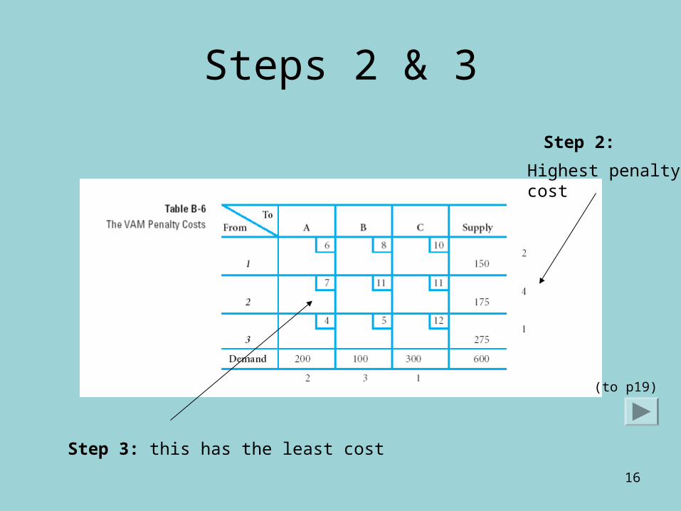
Steps 2 & 3

Highest penaltycost

Step 2:

Step 3: this has the least cost

(to p19)

17

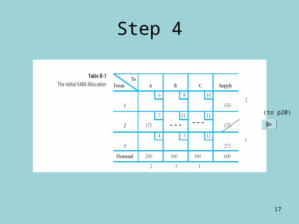
Step 4

--- ---(to p20)

18

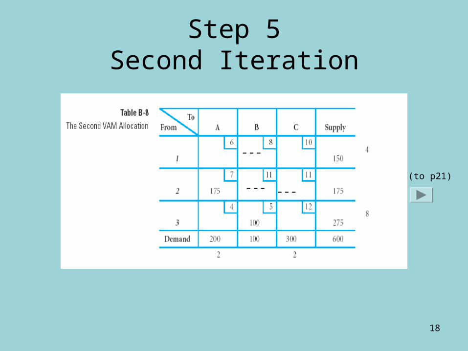
Step 5Second Iteration

--- ---

---

(to p21)

19

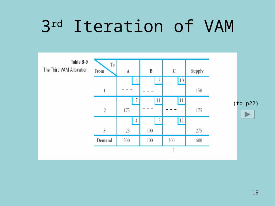
3rd Iteration of VAM

---

--- ---

---

(to p22)

20

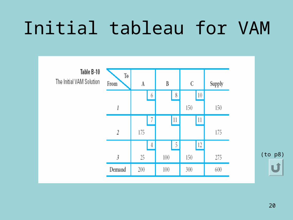
Initial tableau for VAM

(to p8)

21

Optimal solution?

Initial solution from:

Northeast cost, total cost =$5,925

The min cost, total cost =$4,550

VAM, total cost = $5,125(note: here, we are not saying the second one always

better!)

It shows that the second one has the min cost, but is it the optimal solution?

(to p24)

22

Solution methods

• We need a method, like the simplex method, to check and obtain the optimal solution

• Two methods:

1. Stepping-stone method

2. Modified distributed method (MODI)

(to p7)

23

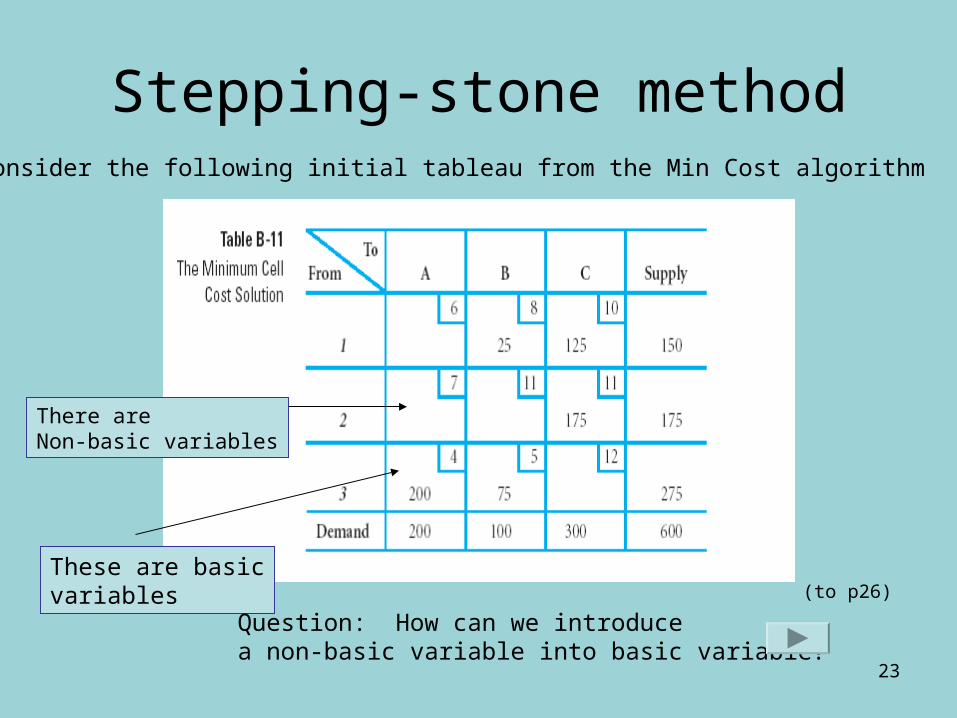
Stepping-stone methodLet consider the following initial tableau from the Min Cost algorithm

These are basicvariables

There areNon-basic variables

Question: How can we introducea non-basic variable into basic variable?

(to p26)

24

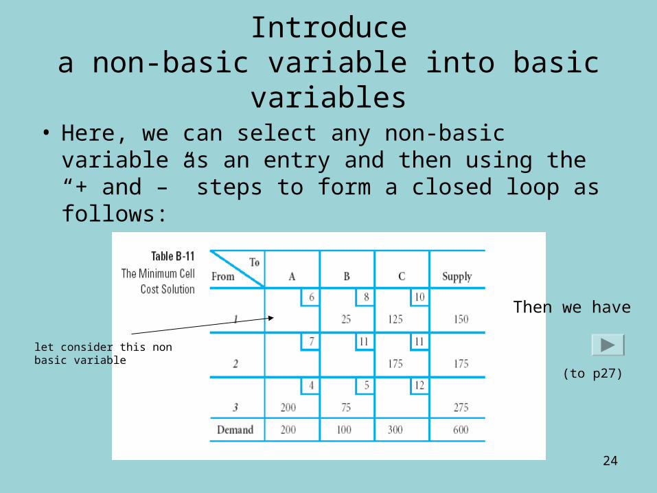
Introducea non-basic variable into basic variables

• Here, we can select any non-basic variable as an entry and then using the “+ and –” steps to form a closed loop as follows:

let consider this nonbasic variable

Then we have

(to p27)

25

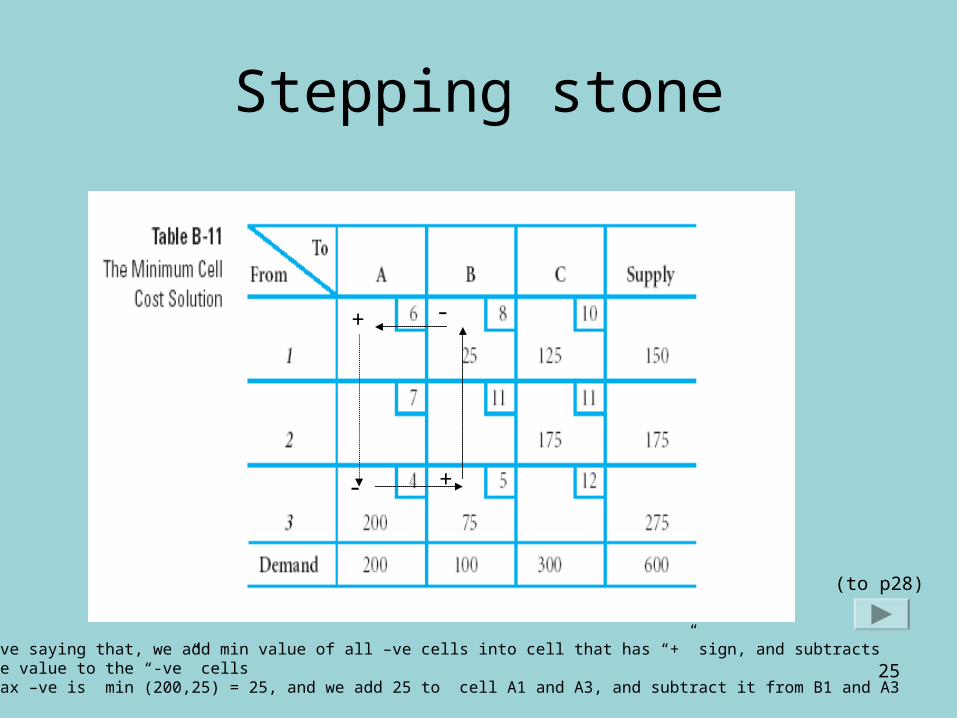
Stepping stone

+

- +

-

The above saying that, we add min value of all –ve cells into cell that has “+” sign, and subtractsthe same value to the “-ve” cellsThus, max –ve is min (200,25) = 25, and we add 25 to cell A1 and A3, and subtract it from B1 and A3

(to p28)

26

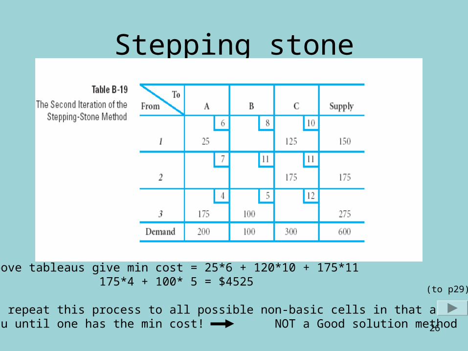
Stepping stone

The above tableaus give min cost = 25*6 + 120*10 + 175*11 175*4 + 100* 5 = $4525

We can repeat this process to all possible non-basic cells in that abovetableau until one has the min cost! NOT a Good solution method

(to p29)

27

Getting optimal solution

• In such, we introducing the next algorithm called Modified Distribution (MODI)

(to p24)

28

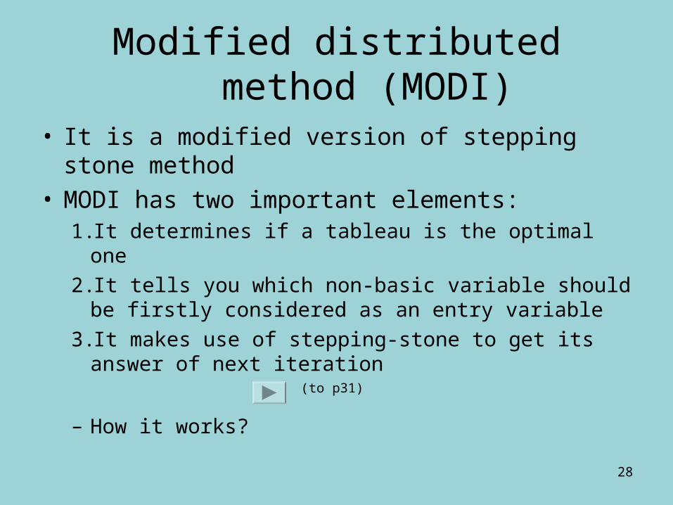
Modified distributed method (MODI)

• It is a modified version of stepping stone method• MODI has two important elements:

1. It determines if a tableau is the optimal one

2. It tells you which non-basic variable should be firstly considered as an entry variable

3. It makes use of stepping-stone to get its answer of next iteration

– How it works? (to p31)

29

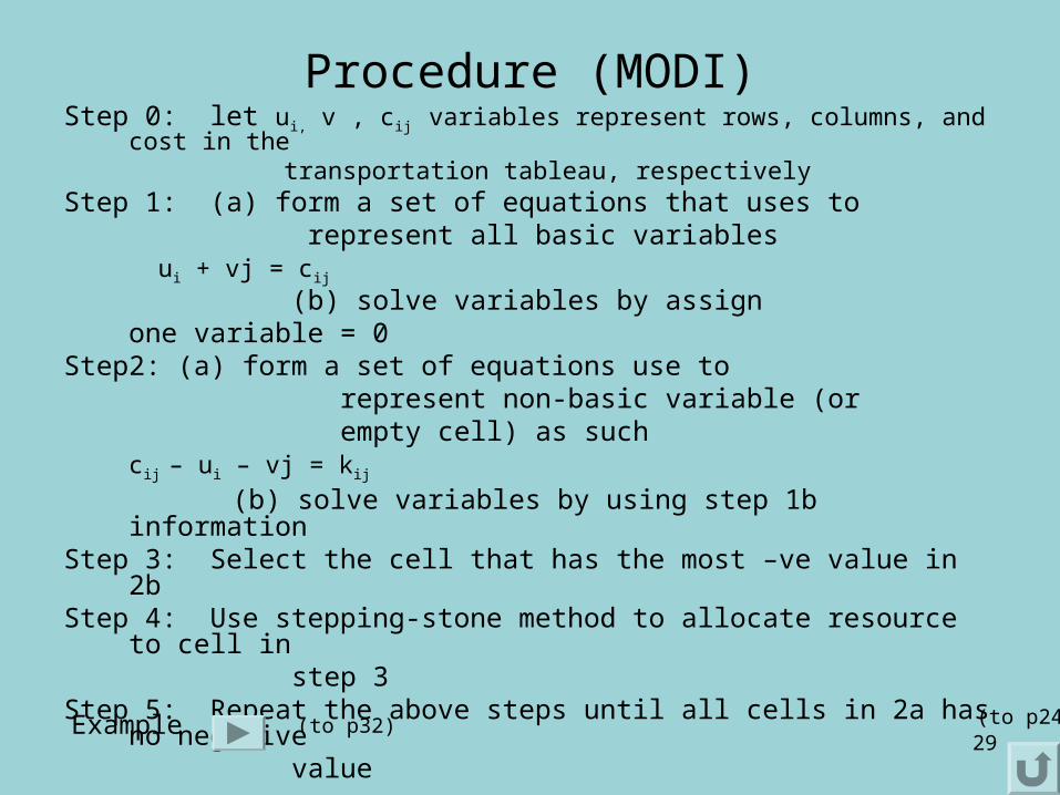
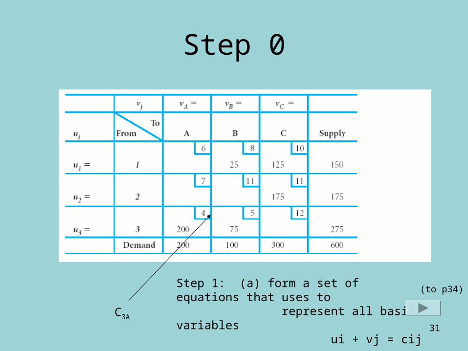
Procedure (MODI)Step 0: let ui, v , cij variables represent rows, columns, and cost in the transportation tableau, respectivelyStep 1: (a) form a set of equations that uses to represent all basic variables

ui + vj = cij

(b) solve variables by assign one variable = 0

Step2: (a) form a set of equations use to represent non-basic variable (or empty cell) as such

cij – ui – vj = kij

(b) solve variables by using step 1b informationStep 3: Select the cell that has the most –ve value in 2bStep 4: Use stepping-stone method to allocate resource to cell in step 3Step 5: Repeat the above steps until all cells in 2a has no negative value

Example (to p24)(to p32)

30

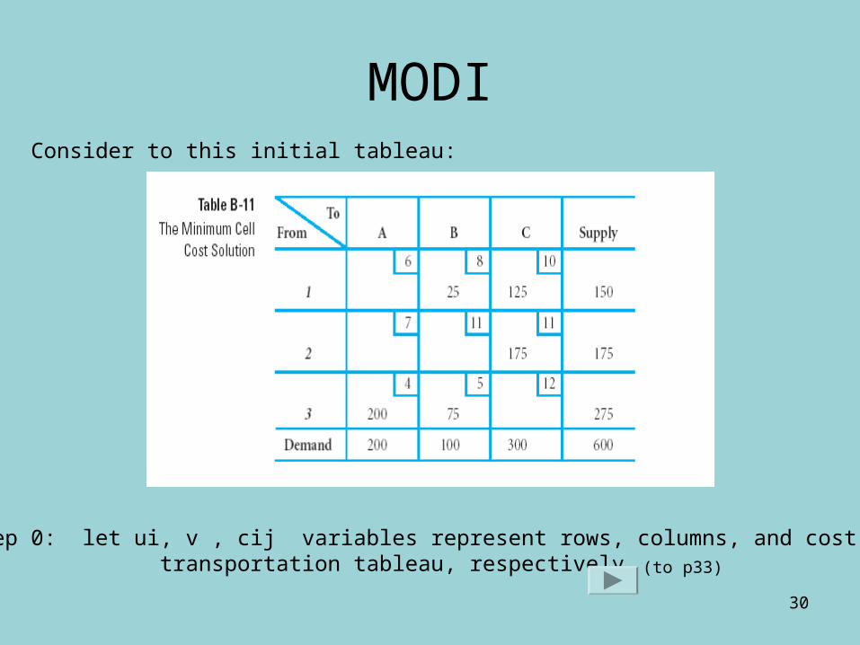
MODIConsider to this initial tableau:

Step 0: let ui, v , cij variables represent rows, columns, and cost in the transportation tableau, respectively (to p33)

31

Step 0

C3A

Step 1: (a) form a set of equations that uses to represent all basic variables

ui + vj = cij

(to p34)

32

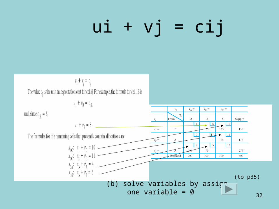
ui + vj = cij

(b) solve variables by assign one variable = 0

(to p35)

33

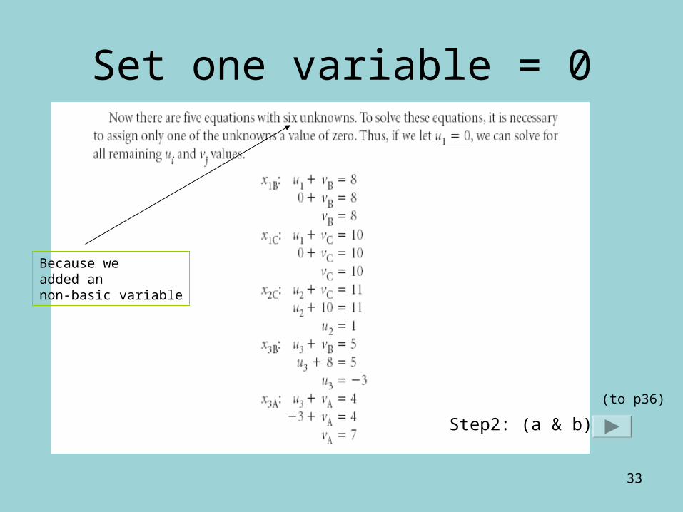
Set one variable = 0

Because weadded an non-basic variable

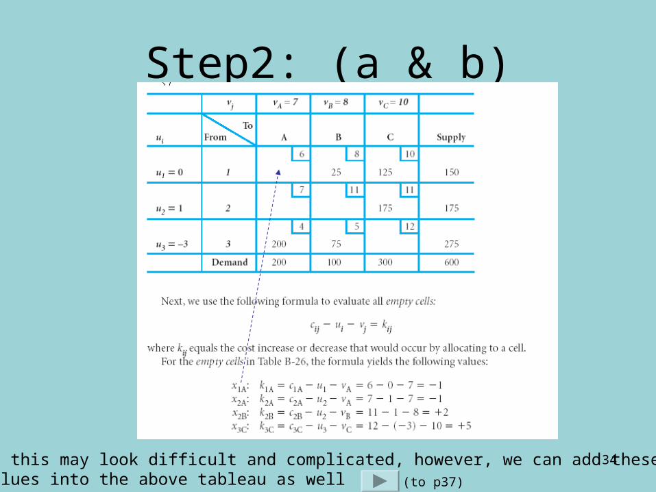
Step2: (a & b)

(to p36)

34

Step2: (a & b)

Note this may look difficult and complicated, however, we can add theseV=values into the above tableau as well (to p37)

35

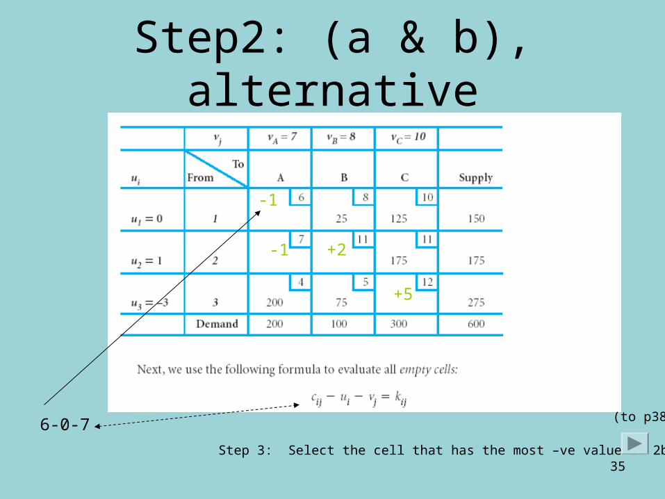
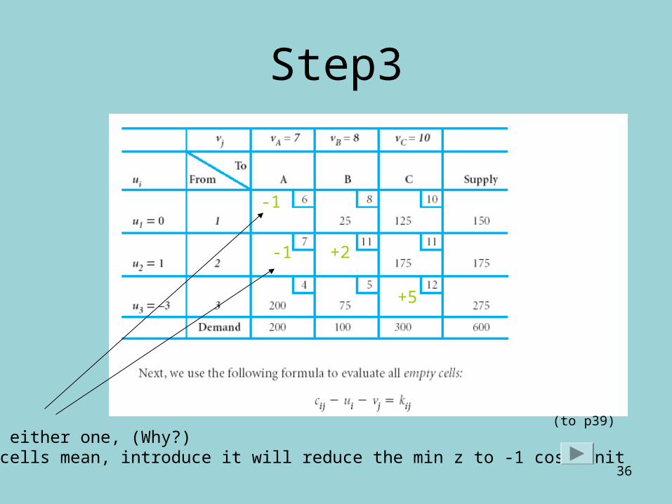
Step2: (a & b), alternative

-1

6-0-7

-1 +2

+5

Step 3: Select the cell that has the most –ve value in 2b

(to p38)

36

Step3

-1

-1 +2

+5

Select either one, (Why?)These cells mean, introduce it will reduce the min z to -1 cost unit

(to p39)

37

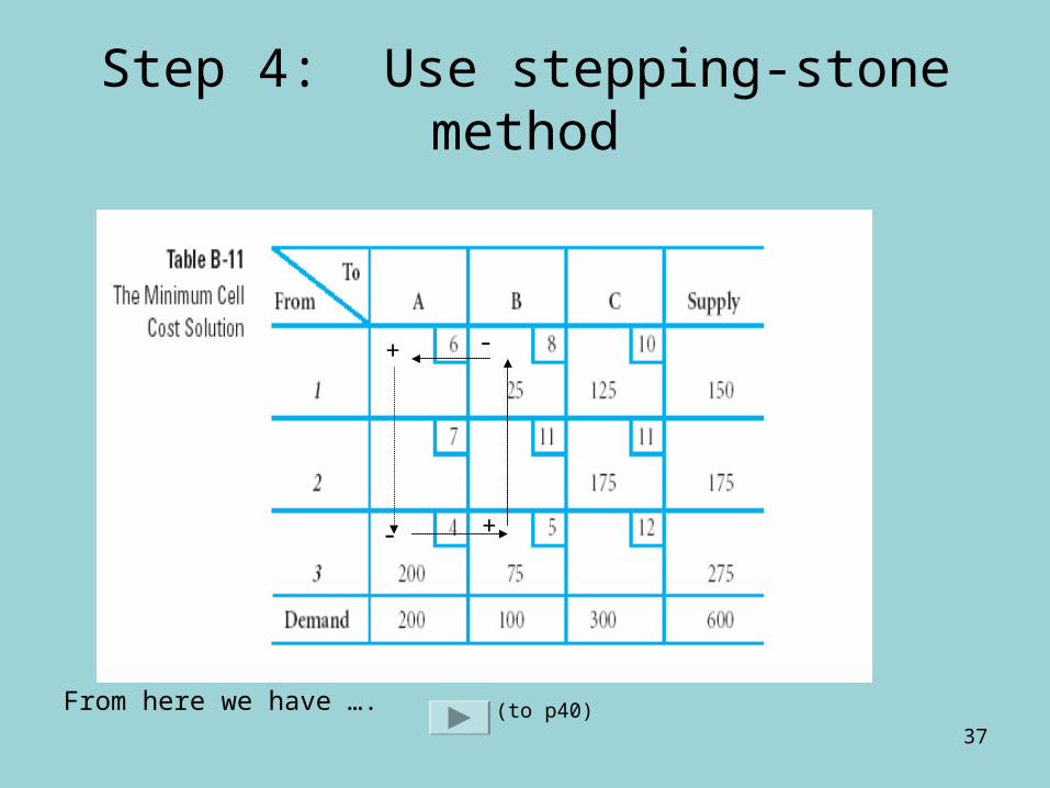
Step 4: Use stepping-stone method

+

- +

-

From here we have …. (to p40)

38

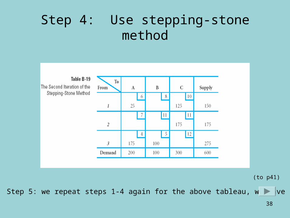
Step 4: Use stepping-stone method

Step 5: we repeat steps 1-4 again for the above tableau, we have

(to p41)

39

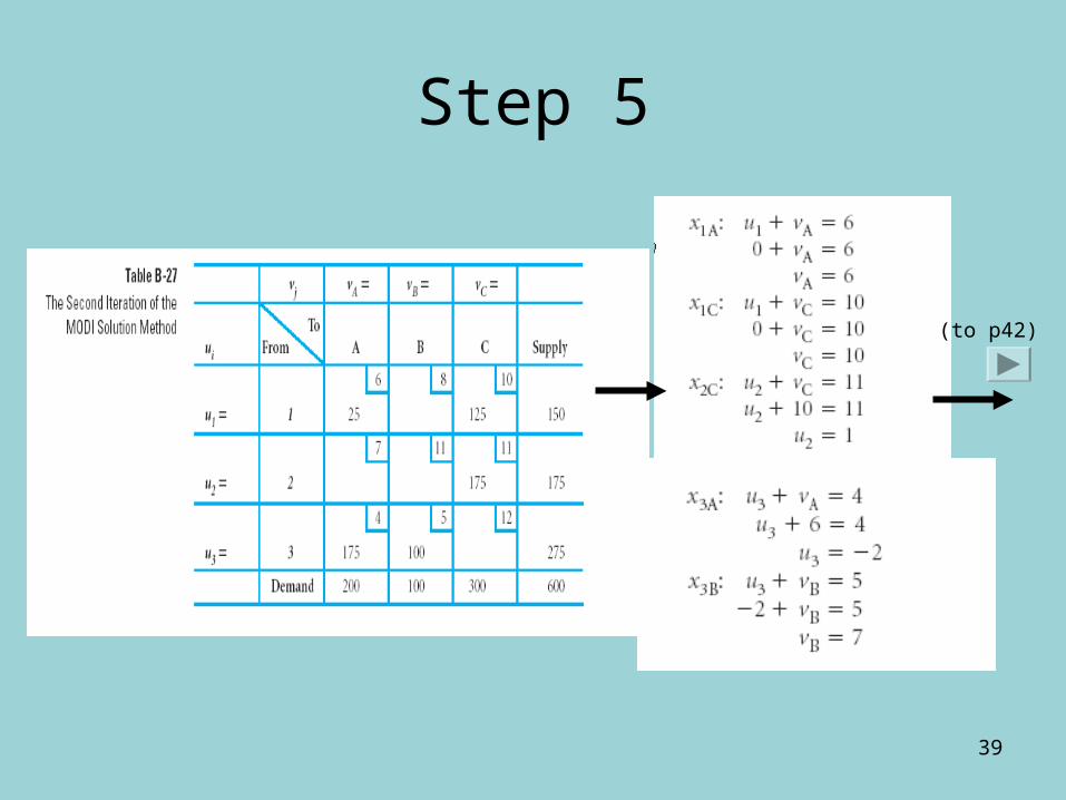
Step 5

(to p42)

40

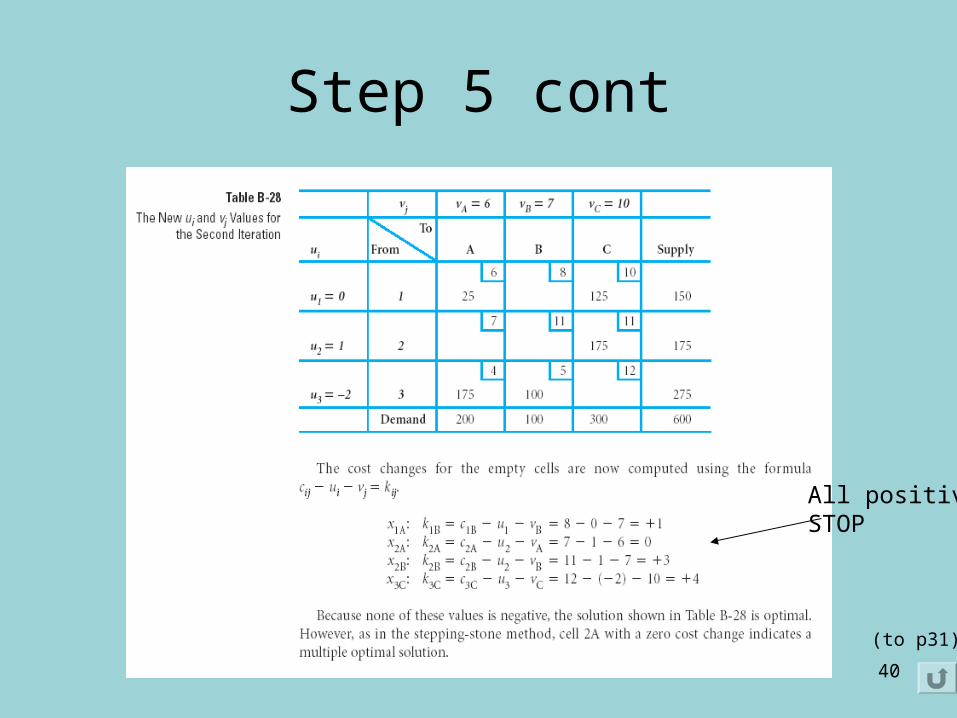
Step 5 cont

All positivesSTOP

(to p31)

41

Important Notes

• When start solving a transportation problem using algorithm, we need to ensure the following:

1. Alternative solution

2. Total demand ≠ total supply

3. Degeneracy

4. others

(to p48)

(to p45)

(to p52)

(to p7)

(to p44)

42

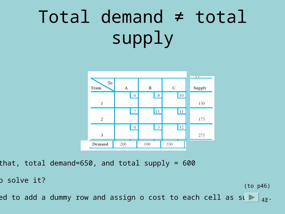
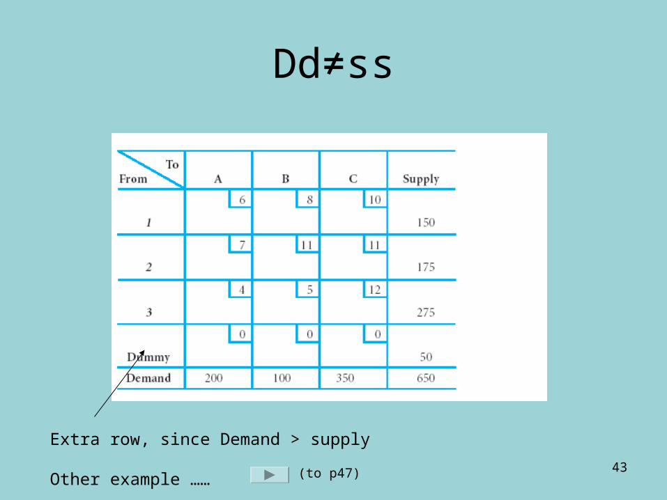
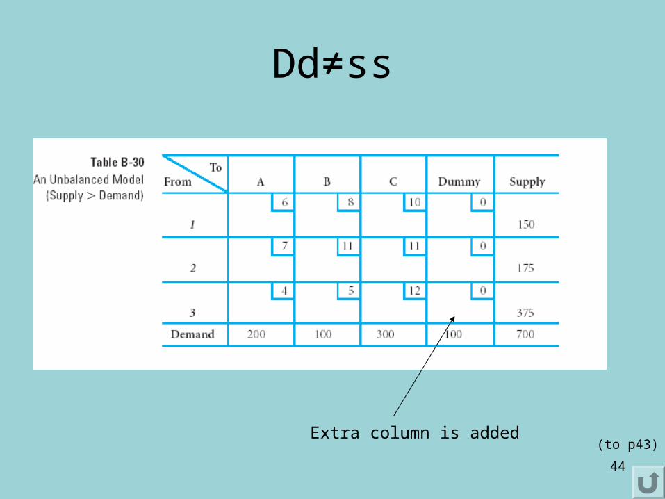
Total demand ≠ total supply

Note that, total demand=650, and total supply = 600

How to solve it?

We need to add a dummy row and assign o cost to each cell as such ..

(to p46)

43

Dd≠ss

Extra row, since Demand > supply

Other example …… (to p47)

44

Dd≠ss

Extra column is added(to p43)

45

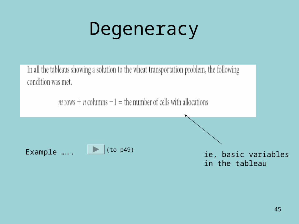
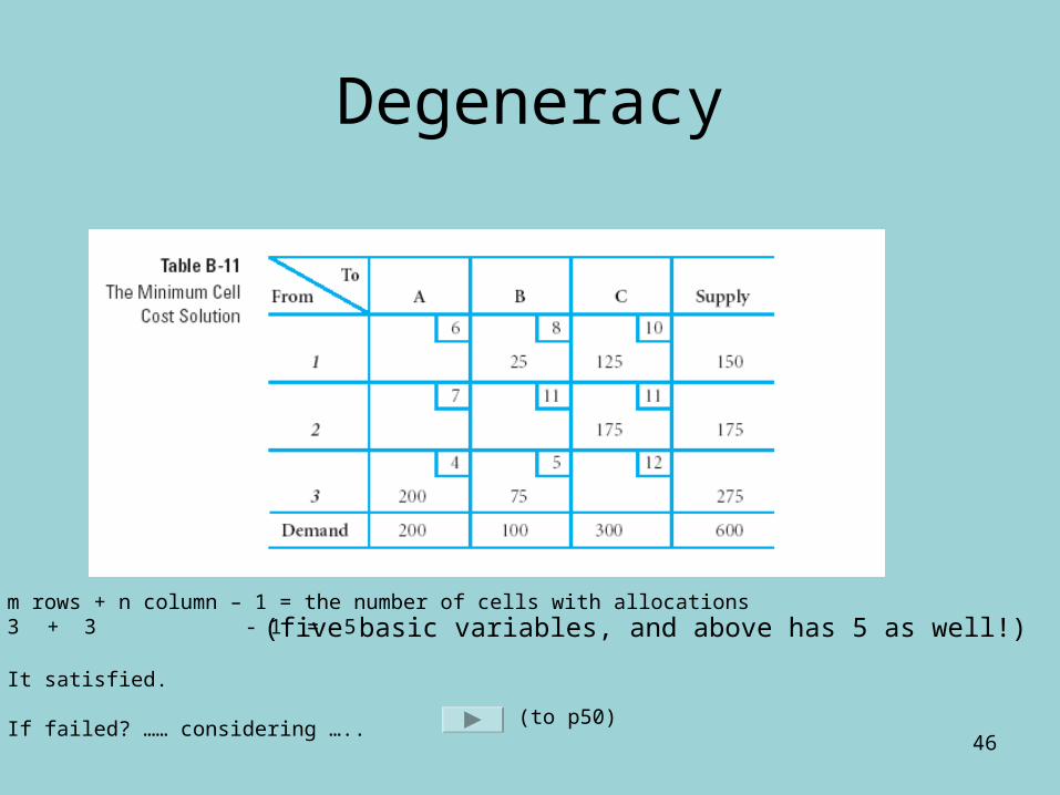
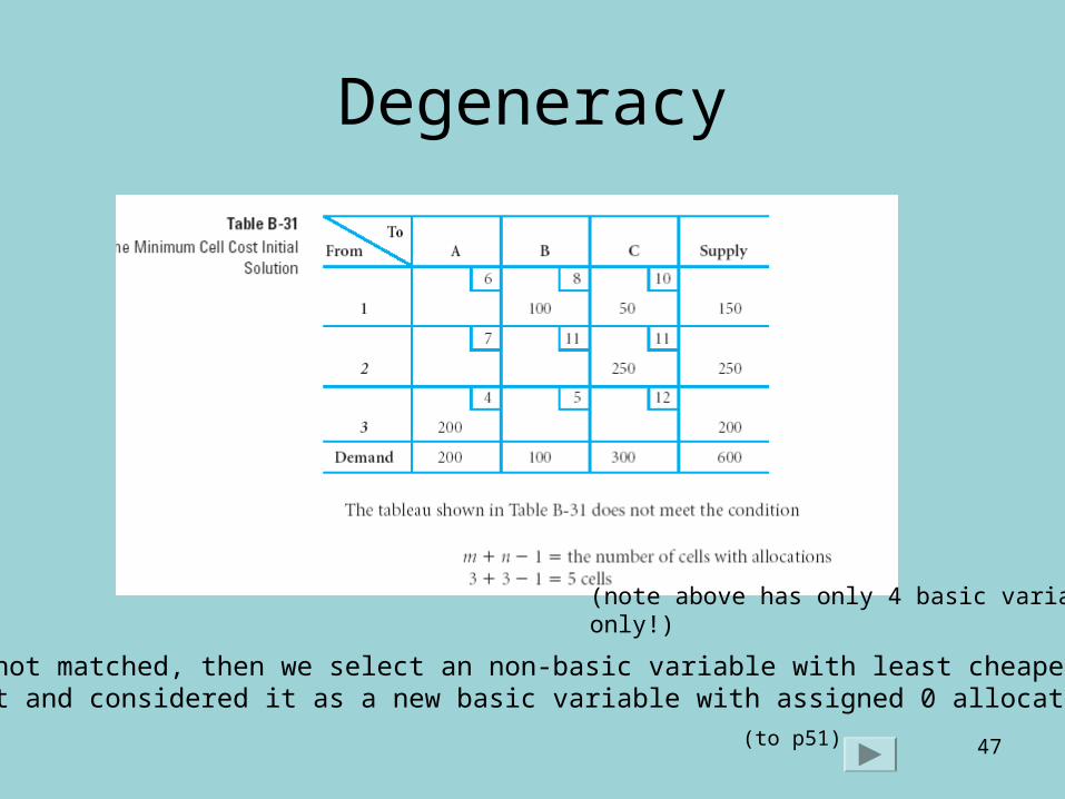
Degeneracy

Example ….. ie, basic variablesin the tableau

(to p49)

46

Degeneracy

m rows + n column – 1 = the number of cells with allocations3 + 3 - 1 = 5

It satisfied.

If failed? …… considering …..

(five basic variables, and above has 5 as well!)

(to p50)

47

Degeneracy

If not matched, then we select an non-basic variable with least cheapest cost and considered it as a new basic variable with assigned 0 allocation to it

(note above has only 4 basic variableonly!)

(to p51)

48

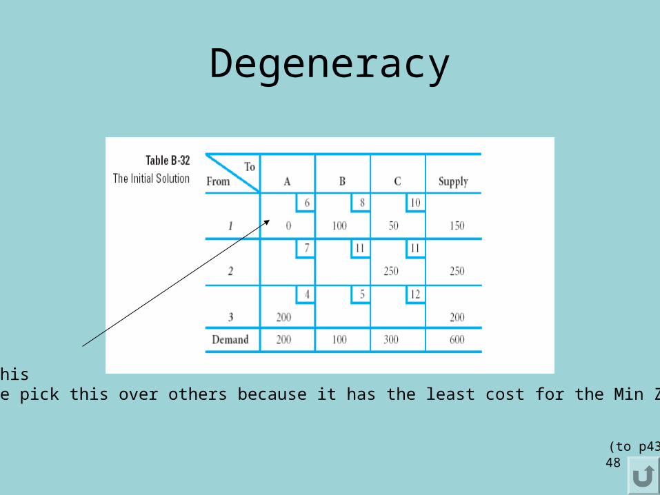
Degeneracy

Added thisNote: we pick this over others because it has the least cost for the Min Z problem!

(to p43)

49

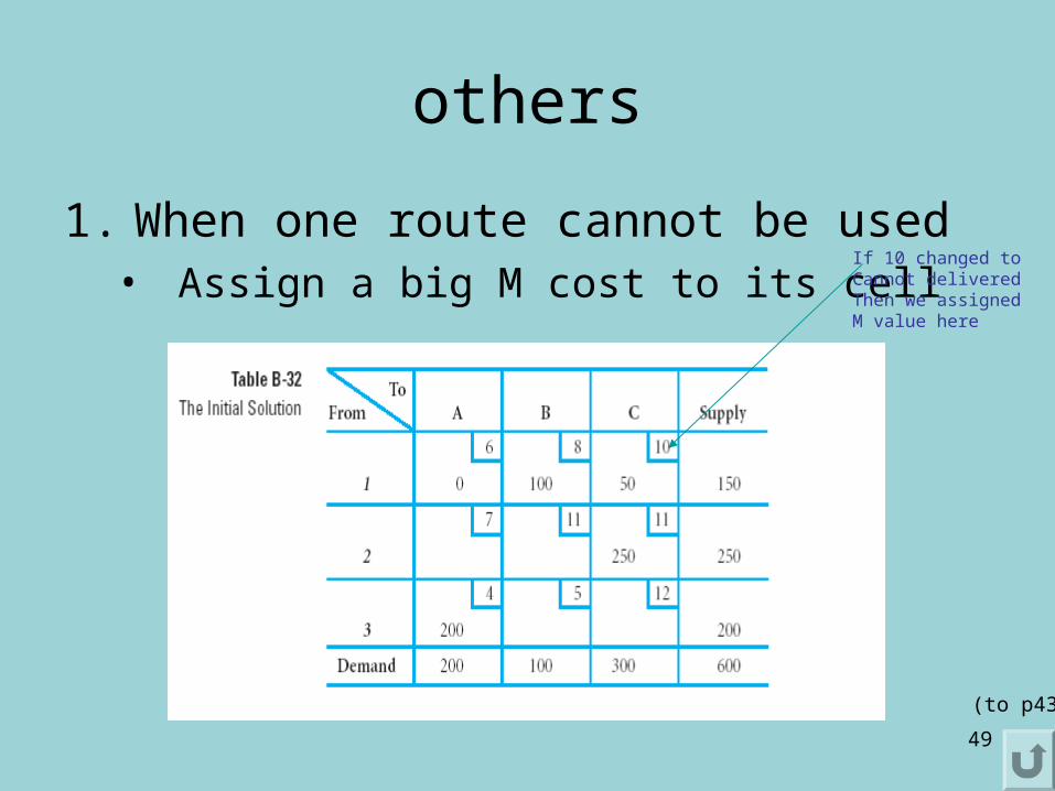
others

1. When one route cannot be used• Assign a big M cost to its cell

(to p43)

If 10 changed to Cannot deliveredThen we assignedM value here