Chapter 7

Transportation, Assignment & Transshipment Problems Part 1

ISE204/IE252 Prof. Dr. Arslan M. ÖRNEK

Warehouse supply of Retail store demand

Television Sets: for television sets:

1 - Cincinnati 300 A - New York 150

2 - Atlanta 200 B - Dallas 250

3 - Pittsburgh 200 C - Detroit 200

Total 700 Total 600

Unit Shipping Costs:

From Warehouse To Store

A B C

1 $16 $18 $11

2 14 12 13

3 13 15 17

Remember from ISE 203:

A Transportation Example

2

Transportation Problem: Characteristics

■ A transportation problem aims to find the best way to fulfill the demand of n demand points using the capacities of m supply points.

■ A product is transported from a number of sources to a number of destinations at the minimum possible cost.

■ Each source is able to supply a fixed number of units of the product, and each destination has a fixed demand for the product.

■ The linear programming model has constraints for supply at each source and demand at each destination.

■ In a balanced transportation model supply equals demand.

3

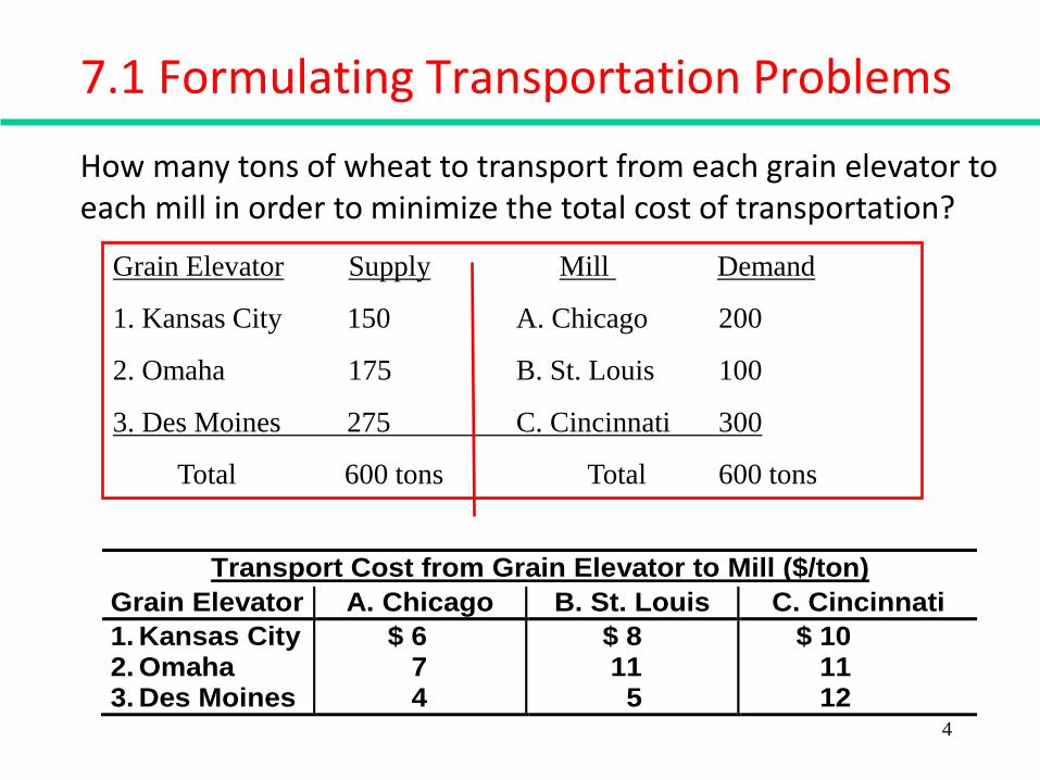
Transport Cost from Grain Elevator to Mill ($/ton)

Grain Elevator A. Chicago B. St. Louis C. Cincinnati

1. Kansas City 2. Omaha 3. Des Moines

$ 6 7 4

$ 8 11

5

$ 10 11 12

How many tons of wheat to transport from each grain elevator to each mill in order to minimize the total cost of transportation?

Grain Elevator Supply Mill Demand

1. Kansas City 150 A. Chicago 200

2. Omaha 175 B. St. Louis 100

3. Des Moines 275 C. Cincinnati 300

Total 600 tons Total 600 tons

7.1 Formulating Transportation Problems

4

Transportation Model Example Transportation Network Routes

Figure 6.1 Network of Transportation Routes for Wheat Shipments 5

xij = tons of wheat from each grain elevator, i, i = 1, 2, 3,

to each mill j = A,B,C Minimize Z = $6x1A + 8x1B + 10x1C + 7x2A + 11x2B + 11x2C + 4x3A + 5x3B + 12x3C

subject to: x1A + x1B + x1C = 150 x2A + x2B + x2C = 175 x3A + x3B + x3C = 275 x1A + x2A + x3A = 200 x1B + x2B + x3B = 100 x1C + x2C + x3C = 300 xij 0

Transportation Model Example Linear Programming Model Formulation

6

Transportation Model Example Optimal Solution

Figure 6.2 Transportation Network Solution 7

7.1 Formulating Transportation Problems Example 1:

Powerco has three electric power plants that supply the electric needs of four cities.

•The associated supply of each plant and demand of each city are known.

•The cost of sending 1 million kwh of electricity from a plant to a city depends on the distance the electricity must travel.

• Formulate an LP to minimize cost.

Solution:

Decision Variable:

x14 = Amount of electricity produced at plant 1 and sent to city 4

Since we want to minimize the total cost of shipping from plants to cities;

Objective Function:

Minimize Z = 8X11+6X12+10X13+9X14+9X21+12X22+13X23+7X24

+14X31 +9X32 +16X33 +5X34

Since each supply point has a limited production capacity;

X11+X12+X13+X14 <= 35

X21+X22+X23+X24 <= 50

X31+X32+X33+X34 <= 40

Since each demand point has a demand to satisfy;

X11+X21+X31 >= 45

X12+X22+X32 >= 20

X13+X23+X33 >= 30

X14+X24+X34 >= 30

Xij >= 0 (i= 1,2,3; j= 1,2,3,4)

Solution (cont):

Supply Constraints

Demand Constraints

Sign Constraints

LP formulation:

Solution (cont):

Network representation of Optimal Solution:

General Description of a Transportation Problem

1. A set of m supply points with a supply of at most si units.

2. A set of n demand points with a demand of at least dj units.

3. Each unit produced at supply point i and shipped to demand point j incurs a variable cost of cij.

xij = number of units shipped from supply point i to demand point j

General Formulation of a Transportation Problem

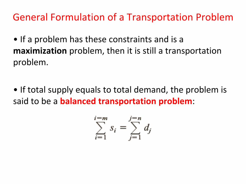
• If a problem has these constraints and is a maximization problem, then it is still a transportation problem.

• If total supply equals to total demand, the problem is said to be a balanced transportation problem:

General Formulation of a Transportation Problem

General Formulation of a Balanced Transportation Problem

It is desirable to formulate a problem as a balanced transportation problem (due to the ease of solution procedures).

Balancing a Transportation Problem if total supply exceeds total demand

If total supply exceeds total demand, we can balance the problem by adding a dummy demand point.

Since shipments to the dummy demand point are not real, they are assigned a cost of zero.

Example 1: Suppose that in the Powerco problem, the demand for city 1 were reduced to 40 million kwh.

To balance the Powerco problem, we would add a dummy demand point (City 5) with a demand of Total Supply – Total Demand = 125 - 120 = 5 million kwh.

From each plant, the cost of shipping 1 million kwh to the dummy is 0.

Balancing a TP if total supply exceeds total demand

Optimal Solution of the Balanced Powerco Problem

Transportation tableau

A transportation problem is specified by the supply, the demand, and the shipping costs. So the relevant data can be summarized in a transportation tableau.

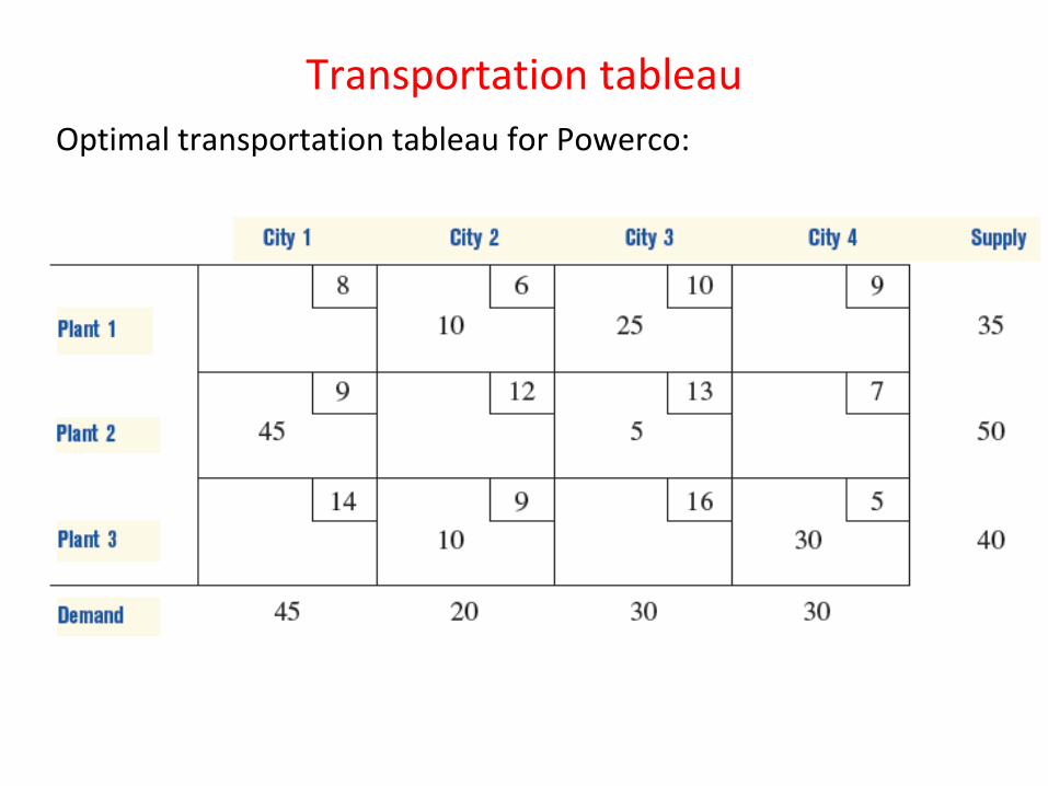
Transportation tableau

Optimal transportation tableau for Powerco:

Balancing a transportation problem if total supply is less than total demand

If total supply < total demand The problem has no feasible solution.

When total supply is less than total demand, it is sometimes desirable to allow the possibility of leaving some demand unsatisfied. In such a situation, a penalty is often associated with unmet demand.

• Example 2 (Handling Shortages):

23

• Solution:

24

25

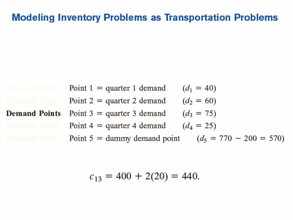
Sailco Corporation must determine how many sailboats should be produced during each of the next four quarters (one quarter is three months).

Demand : first quarter, 40 sailboats; second quarter, 60 sailboats; third quarter, 75 sailboats; fourth quarter, 25 sailboats.

Sailco must meet demand on time. At the beginning of the first quarter, Sailco has an inventory of 10 sailboats.

At the beginning of each quarter, Sailco must decide how many sailboats should be produced during the current quarter.

For simplicity, we assume that sailboats manufactured during a quarter can be used to meet the demand for that quarter.

During each quarter, Sailco can produce up to 40 sailboats at a cost of $400 per sailboat. By having employees work overtime during a quarter, Sailco can produce additional sailboats at a cost of $450 per sailboat.

At the end of each quarter (after production has occurred and the current quarter’s demand has been satisfied), a carrying or holding cost of $20 per sailboat is incurred.

Formulate a balanced transportation problem to minimize the sum of production and inventory costs during the next four quarters.

Capacity of each OT supply point = 150 =

200 (Total demand) – 10 (initial

inventory) – 40 (regular time production

capacity)

7.2 Finding Basic Feasible Solution for TP

A balanced TP with m supply points and n demand points is easier to solve than a regular LP, although it has m + n equality constraints.

If a set of values for the xij’s satisfies all but one of the constraints of a balanced transportation problem, then the values for the xij’s will automatically satisfy the other constraint.

This means that only m+n-1 constraints are linearly independent. m+n-1 basic variables

Methods to find the bfs for a balanced TP

There are three basic methods:

1. Northwest Corner Method

2. Minimum Cost Method

3. Vogel’s Method

1. Northwest Corner Method (NWC)

To find the bfs by the NWC method:

Begin in the upper left (northwest) corner of the transportation tableau and set x11 as large as possible (the limitations for setting x11 will be the demand of demand point 1 and the supply of supply point 1. Your x11 value can not be greater than the minimum of this two values).

Example: Set x11=3 (meaning demand of demand point 1 is satisfied by supply point 1).

5

6

2

3 5 2 3

3 2

6

2

X 5 2 335

After we check the east and south cells, we see that we can go east (meaning supply point 1 still has capacity to fulfill some demand).

3 2 X

6

2

X 3 2 3

3 2 X

3 3

2

X X 2 336

After applying the same procedure, we see that we can go south this time (meaning demand point 2 needs more supply by supply point 2).

3 2 X

3 2 1

2

X X X 3

3 2 X

3 2 1 X

2

X X X 2 37

Finally, we will have the following bfs: x11=3, x12=2, x22=3, x23=2, x24=1, x34=2

3 2 X

3 2 1 X

2 X

X X X X

38

Example:

39

Example:

Supply and

demand

equal, cross

only one,

not both!

40

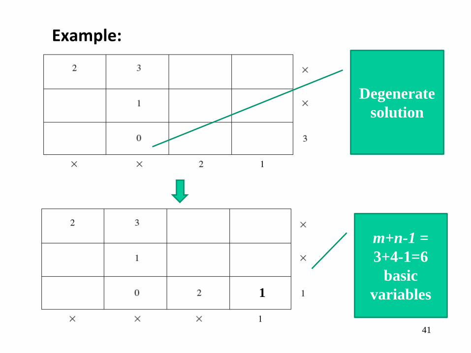
Example:

Degenerate

solution

1

m+n-1 =

3+4-1=6

basic

variables

41

2. Minimum Cost Method

The Northwest Corner Method does not utilize shipping costs. It can yield an initial bfs easily but the total shipping cost may be very high.

The minimum cost method uses shipping costs in order come up with a bfs that has a lower cost. To begin the minimum cost method, first we find the decision variable with the smallest shipping cost.

Then assign xij its largest possible value, which is the minimum of si and dj.

Cross out the row or column, then continue with the next minimum cost.

Example: Step 1: Select the cell with minimum cost.

2 3 5 6

2 1 3 5

3 8 4 6

5

10

15

12 8 4 6

Step 2: Cross-out column 2

2 3 5 6

2 1 3 5

8

3 8 4 6

12 X 4 6

5

2

15

44

Step 3: Find the new cell with minimum shipping cost and cross-out row 2

2 3 5 6

2 1 3 5

2 8

3 8 4 6

5

X

15

10 X 4 6

45

Step 4: Find the new cell with minimum shipping cost and cross-out row 1

2 3 5 6

5

2 1 3 5

2 8

3 8 4 6

X

X

15

5 X 4 6

46

Step 5: Find the new cell with minimum shipping cost and cross-out column 1

2 3 5 6

5

2 1 3 5

2 8

3 8 4 6

5

X

X

10

X X 4 6

47

Step 6: Find the new cell with minimum shipping cost and cross-out column 3

2 3 5 6

5

2 1 3 5

2 8

3 8 4 6

5 4

X

X

6

X X X 6

48

Step 7: Finally assign 6 to last cell. The bfs is found as: X11=5, X21=2, X22=8, X31=5, X33=4 and X34=6

2 3 5 6

5

2 1 3 5

2 8

3 8 4 6

5 4 6

X

X

X

X X X X

49

3. Vogel’s Method

Begin with computing each row and column a penalty. The penalty will be equal to the difference between the two smallest shipping costs in the row or column.

Identify the row or column with the largest penalty. Find the first basic variable which has the smallest shipping cost in that row or column. Then assign the highest possible value to that variable, and cross-out the row or column as in the previous methods.

Compute new penalties and use the same procedure.

Example: Step 1: Compute the penalties.

Supply Row Penalty

6 7 8

15 80 78

Demand

Column Penalty 15-6=9 80-7=73 78-8=70

7-6=1

78-15=63

15 5 5

10

15

51

Step 2: Identify the largest penalty and assign the highest possible value to the least-cost variable.

Supply Row Penalty

6 7 8

5

15 80 78

Demand

Column Penalty 15-6=9 _ 78-8=70

8-6=2

78-15=63

15 X 5

5

15

52

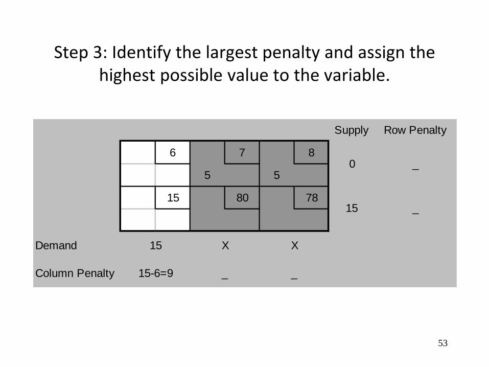
Step 3: Identify the largest penalty and assign the highest possible value to the variable.

Supply Row Penalty

6 7 8

5 5

15 80 78

Demand

Column Penalty 15-6=9 _ _

_

_

15 X X

0

15

53

Step 4: Identify the largest penalty and assign the highest possible value to the variable.

Supply Row Penalty

6 7 8

0 5 5

15 80 78

Demand

Column Penalty _ _ _

_

_

15 X X

X

15

54

Step 5: Finally the bfs is found as X11=0, X12=5, X13=5, and X21=15

Supply Row Penalty

6 7 8

0 5 5

15 80 78

15

Demand

Column Penalty _ _ _

_

_

X X X

X

X

55