Transportation and power solutions for Africa: The ...

Purdue UniversityPurdue e-Pubs

Open Access Theses Theses and Dissertations

4-2016

Transportation and power solutions for Africa: Theassessment and optimization of the Purdue utilityplatformJeremy Patrick RobisonPurdue University

Follow this and additional works at: https://docs.lib.purdue.edu/open_access_theses

Part of the Automotive Engineering Commons, and the Mechanical Engineering Commons

This document has been made available through Purdue e-Pubs, a service of the Purdue University Libraries. Please contact [email protected] foradditional information.

Recommended CitationRobison, Jeremy Patrick, "Transportation and power solutions for Africa: The assessment and optimization of the Purdue utilityplatform" (2016). Open Access Theses. 808.https://docs.lib.purdue.edu/open_access_theses/808

https://docs.lib.purdue.edu?utm_source=docs.lib.purdue.edu%2Fopen_access_theses%2F808&utm_medium=PDF&utm_campaign=PDFCoverPages

https://docs.lib.purdue.edu/open_access_theses?utm_source=docs.lib.purdue.edu%2Fopen_access_theses%2F808&utm_medium=PDF&utm_campaign=PDFCoverPages

https://docs.lib.purdue.edu/etd?utm_source=docs.lib.purdue.edu%2Fopen_access_theses%2F808&utm_medium=PDF&utm_campaign=PDFCoverPages

https://docs.lib.purdue.edu/open_access_theses?utm_source=docs.lib.purdue.edu%2Fopen_access_theses%2F808&utm_medium=PDF&utm_campaign=PDFCoverPages

http://network.bepress.com/hgg/discipline/1319?utm_source=docs.lib.purdue.edu%2Fopen_access_theses%2F808&utm_medium=PDF&utm_campaign=PDFCoverPages

http://network.bepress.com/hgg/discipline/293?utm_source=docs.lib.purdue.edu%2Fopen_access_theses%2F808&utm_medium=PDF&utm_campaign=PDFCoverPages

https://docs.lib.purdue.edu/open_access_theses/808?utm_source=docs.lib.purdue.edu%2Fopen_access_theses%2F808&utm_medium=PDF&utm_campaign=PDFCoverPages

Graduate School Form30 Updated

PURDUE UNIVERSITYGRADUATE SCHOOL

Thesis/Dissertation Acceptance

This is to certify that the thesis/dissertation prepared

By

Entitled

For the degree of

Is approved by the final examining committee:

To the best of my knowledge and as understood by the student in the Thesis/Dissertation Agreement, Publication Delay, and Certification Disclaimer (Graduate School Form 32), this thesis/dissertation adheres to the provisions of Purdue University’s “Policy of Integrity in Research” and the use of copyright material.

Approved by Major Professor(s):

Approved by:Head of the Departmental Graduate Program Date

JEREMY PATRICK ROBISON

TRANSPORTATION AND POWER SOLUTIONS FOR AFRICA: THE ASSESSMENT AND OPTIMIZATION OF THEPURDUE UTILITY PLATFORM

Master of Science in Engineering

John LumkesChair

John Starkey Co-chair

Dennis BuckmasterCo-chair

John Lumkes

Bernard Engel 4/18/2016

i

i

TRANSPORTATION AND POWER SOLUTIONS FOR AFRICA: THE

ASSESSMENT AND OPTIMIZATION OF THE PURDUE UTILITY PLATFORM

A Thesis

Submitted to the Faculty

of

Purdue University

by

Jeremy Patrick Robison

In Partial Fulfillment of the

Requirements for the Degree

of

Master of Science in Engineering

May 2016

Purdue University

West Lafayette, Indiana

ii

ii

ACKNOWLEDGEMENTS

Working on this thesis has been an incredible journey as it has taken me all over the

world as our team of Purdue faculty, staff, and students work toward implementing the

PUP in sub-Saharan Africa. This journey has not always been easy, and I have had many

challenging days, but help and support from several wonderful people and organizations

have helped see me through it. To begin, I want to thank the John Deere Foundation, I2D

Lab, the Purdue Office of Engagement, and the Purdue Global Engineering Program for

supporting my work financially and logistically. Your efforts have greatly impacted the

success of the PUP project’s work. Also, I want to thank my parents John and Marilyn

Robison for their patience and for being my constant source of love and support. Dr.

Lumkes has been a great teacher and mentor throughout this process, and I want to thank

him for this opportunity, for his patience, for his encouragement, and for his support

throughout this journey. Also, I want to thank Amanda Emery and Colin Lawrence for

being wonderful people and always helping me out when I needed it. I also want to thank

the good people in my graduate community who have helped me be successful in this

work and have made it a lot of fun along the way. Thank you David Wilson, Jordan

Garrity, Farid Breidi, Tyler Helmus, Gabe Wilfong, and Arnav Gupta for all of your help.

Finally and ultimately, “Not to us, Lord, not to us but to your name be the glory, because

of your love and faithfulness” Psalm 115.

iii

iii

TABLE OF CONTENTS

Page

LIST OF TABLES .............................................................................................................. v

LIST OF FIGURES ......................................................................................................... viii

LIST OF ABBREVIATIONS ........................................................................................... xv

ABSTRACT ..................................................................................................................... xvi

CHAPTER 1. INTRODUCTION .................................................................................... 1

1.1 The World Food Challenge ....................................................................................... 1

1.2 Agricultural Mechanization and Productivity ........................................................... 2

1.3 Transportation Challenges ......................................................................................... 3

1.4 The Purdue Utility Platform ...................................................................................... 4

1.5 Scope of Work ........................................................................................................... 6

CHAPTER 2. BACKGROUND RESEARCH................................................................. 7

2.1 History of Agricultural Mechanization ..................................................................... 7

2.2 Agricultural Mechanization in Sub-Saharan Africa .................................................. 9

2.3 Benefits of Agricultural Mechanization .................................................................. 11

2.4 Transportation in Sub-Saharan Africa ..................................................................... 13

2.5 The Purdue Utility Platform .................................................................................... 20

2.5.1 The Reason and Introduction for the Purdue Utility Platform ...................... 20

2.5.2 The History of the Purdue Utility Platform ................................................... 21

2.5.3 Specifications for 2015 PUP .......................................................................... 32

2.5.4 Technical Lessons Learned ............................................................................ 33

2.6 Truss Frame Research ............................................................................................. 33

2.6.1 Truss Frame Fundamentals ............................................................................ 33

2.6.2 Types of Trusses and Applications ................................................................ 34

iv

iv

Page

2.6.3 Analysis of Space Frames .............................................................................. 36

2.6.4 Three Wheeled Vehicle Dynamics ................................................................ 38

CHAPTER 3. FRAME STUDY AND VEHICLE DYNAMICS METHODS .............. 42

3.1 Introduction to Methodology .................................................................................. 42

3.2 Vehicle Frame Design Improvements ..................................................................... 42

3.3 Vehicle Data Acquisition ........................................................................................ 47

3.3.1 Importance of Data Acquisition ..................................................................... 47

3.3.2 Applications of a PUP DAQ System ............................................................. 48

3.3.3 Data Acquisition for Measuring Frame Stress and Validating FEA Models 50

3.4 FEA Model Study .................................................................................................... 57

3.5 Rolling Stability Simulation .................................................................................... 60

3.6 Summary ................................................................................................................. 69

CHAPTER 4. RESULTS AND DISCUSSION ON THE FRAME AND ROLL

STABILITY STUDY........................................................................................................ 71

4.1 Introduction ............................................................................................................. 71

4.2 Frame Study Results ................................................................................................ 71

4.2.1 Strain Gauge Data .......................................................................................... 71

4.2.2 FEA Model Validation .................................................................................. 81

4.3 Roll Stability Results ............................................................................................... 88

4.3.1 Introduction to Roll Stability Study ............................................................... 88

4.3.2 Maximum Lateral Acceleration Boundaries .................................................. 89

CHAPTER 5. SUMMARY OF WORK ....................................................................... 113

5.1 Strain Gauge and Video Study Findings ............................................................... 113

5.1.1 Frame Study Design Tools .......................................................................... 113

5.1.2 Frame Study Durability Conclusions ........................................................... 116

5.2 Roll Stability Findings .......................................................................................... 118

WORKS CITED ............................................................................................................. 124

APPENDIX ..................................................................................................................... 128

v

v

LIST OF TABLES

Table .............................................................................................................................. Page

Table 1 - Motor Vehicles Per 1000 People In Sub-Saharan Africa (ChartsBin, 2011) .... 14

Table 2 - Comparison of Rural Transport (Riverson & Carapetis, 1991) ........................ 19

Table 3 - 2011 PUP Specifications (Lumkes, 2012)......................................................... 25

Table 4 - 2015 PUP Specifications ................................................................................... 32

Table 5 – Description of Symbols for Six Degree of Freedom Model ............................. 65

Table 6 – Average Experimental Stress Values for the Front Strut 2 Location While

Driving the PUP Unloaded Over a Single Concrete Stop (Excludes Static Weight Stress)

........................................................................................................................................... 81

Table 7 – Comparison of Experimental and ANSYS Simulated Stress for the Left

Trailing Arm Location for when the Two Rear Wheels Drive over a Concrete Stop ...... 83


Trailing Arm Location for when the Left Rear Wheel Drives over a Concrete Stop When

the PUP is Unloaded ......................................................................................................... 85

Table 9 – Frame Study Summary with Static Stress Included for the Front Strut 2 Strain

Gauge Location for When an Unloaded PUP’s Front Tire First Collides with a Concrete

Stop (Stress Values Include the Stress From the Static Weight of the Vehicle) ............. 88

vi

vi

Table .............................................................................................................................. Page

Table 10 - Frame Study Summary with Static Stress Included for the Front Strut 2 Strain

Gauge Location for When an Unloaded PUP’s Front Tire Rolls off the Concrete Stop and

Lands on The Ground (Stress Values Include the Stress From the Static Weight of the

Vehicle) ............................................................................................................................. 88

Table 11 - Measured PUP Values and CG Locations (for geometry reference see figure

57) ..................................................................................................................................... 90

Table 12 - Measured Spring Rates .................................................................................... 91

Table 13 - Summary of Braking and Accelerating Simulations ..................................... 104

Table 14 - Roll Stability Study with Varying Braking Scenarios ................................... 108

Table 15 – Left Trailing Arm with No Load - Two Wheel Bump Summary ................. 113

Table 16 – Left Trailing Arm with No Load - One Wheel Bump Summary .................. 114

Table 17 – Summary of the Frame Study Comparing Experimental and Simulated Stress

Values at the Front Strut Frame Member for When the Front Tire Initially Hits a

Concrete Stop .................................................................................................................. 115


Values at the Front Strut Frame Member for When the Front Tire Lands on the Ground

on the Other Side of a Concrete Stop .............................................................................. 115

Table 19 – Vehicle Vertical and Longitudinal Static Mass Acceleration Estimates ...... 116

Table 20 – Endurance Limits For SAE 1020 Steel PUP Members ................................ 118

Table 21 – Description of Symbols for Equation 42 ...................................................... 120

Table 22 - Simulation Results for Wheel Liftoff Events for an Unloaded PUP ............. 122

vii

vii

Appendix Table .............................................................................................................. Page

Table A 1- Left Trailing Arm - No Load - Single Tire Bump Test Stress Summary ..... 129

Table A 2 - Left Trailing Arm - 1500 lb Load - Single Tire Bump Test Stress Summary

......................................................................................................................................... 129

Table A 3 – Roll Stability Dynamic Simulation Parameters .......................................... 130

viii

viii

LIST OF FIGURES

Figure ............................................................................................................................. Page

Figure 1 - 2014 PUP Frame Failure .................................................................................... 5

Figure 2 - Motorbike Used in Cameroon – source: PUP Drive ........................................ 16

Figure 3 - Auto Rickshaw or Tuk-Tuk (Lovson, 2016) .................................................... 17

Figure 4 - Kavaki Motor Chinese Trike ("Alibaba Manufacturer Directory - Suppliers,

Manufacturers, Exporters & Importers," 2016) ................................................................ 17

Figure 5 - Two Wheel Multi-Function Tractor with Seat Attachment (Alibaba, 2016) ... 18

Figure 6 - 2010 PUP with Wooden Frame........................................................................ 23

Figure 7 - 2011 PUP in Cameroon .................................................................................... 25

Figure 8 - 2012 PUP at ACREST in Cameroon ............................................................... 27

Figure 9 - Maize Grinder Attachment (Top Left), Water Pump Attachment (Top Right),

and Planter (Bottom) ......................................................................................................... 27

Figure 10 - 2013 PUP in Cameroon .................................................................................. 29

Figure 11 - 2014 PUP at Purdue ....................................................................................... 30

Figure 12 - 2015 PUP in Cameroon .................................................................................. 31

Figure 13 – 2015 PUP Dimensions ................................................................................... 32

Figure 14 - Simple Truss (Connor & Faraji, 2012) .......................................................... 34

Figure 15 - Types of Truss Shapes (Connor & Faraji, 2012) ........................................... 34

ix

ix

Figure ............................................................................................................................. Page

Figure 16 - Warren Type Airplane Fuselage (United States. Flight Standards et al., 2012)

........................................................................................................................................... 35

Figure 17 - Jaguar C – Type with Space Frame (Classics, 2016) ..................................... 36

Figure 18 - Frame Finite Element Model Loading Case(Riley & George, 2002) ............ 38

Figure 19 - Four Wheeled vs Three Wheeled Roll Dynamics .......................................... 39

Figure 20 – Three Wheel Vehicle Symbol Explanation ................................................... 41

Figure 21 - Powertrain Tunnel .......................................................................................... 43

Figure 22 - Functionality Frame Changes ........................................................................ 44

Figure 23 - 2014 PUP Frame Failure on Front Strut Lateral Member.............................. 44

Figure 24 - 2013 PUP Driver Seat and Trailing Arm Failure ........................................... 45

Figure 25 - 2012 PUP Frame Failure on Front Strut Angle Iron ...................................... 45

Figure 26 - Frame Strengthening Additions ..................................................................... 46

Figure 27 - ANSYS Solution for Combined Loading ...................................................... 47

Figure 28 - Red Board DAQ System ................................................................................ 49

Figure 29 - GPS Data Collected With TK103A Vehicle Tracker .................................... 50

Figure 30 - A Precision Strain Gauge Mounted To One of the Front Strut Angle Iron

Members ........................................................................................................................... 51

Figure 31 – Half Bridge Configuration Type 1(Instruments, 2016) ................................. 52

Figure 32 - Front Panel of Strain Gauge vi File................................................................ 53

Figure 33 – Data Acquisition Helper ................................................................................ 54

Figure 34 –Video of Strain Gauge Experiment (left) Camera and Wheatstone Bridge

Mounting (right)................................................................................................................ 55

x

x

Figure ............................................................................................................................. Page

Figure 35 - Strain Gauge Placement ................................................................................. 56

Figure 36 – ANSYS Static Structural Model Considering a Two Wheel Collision ......... 59

Figure 37 – Three Wheel Vehicle Model with Six Degrees of Freedom (Raman et al.,

1995) ................................................................................................................................. 61

Figure 38 – Lateral Force vs Slip Angle “x” (left) and Cornering Stiffness vs Fz (right) 67

Figure 39 - Cornering Stiffness Curve Produced By Magic Formula for Simulation ...... 68

Figure 40 - Lateral Force Curves Produced By Magic Formula ...................................... 68

Figure 41 – Strain Gauge Values for the Front Strut 1 Location While the PUP is

Unloaded and Driving over Two Concrete Stops and Large Gravel ................................ 73


operating without a Load in the Bed While Driving over a Concrete Stop ...................... 73

Figure 43 - Strain Gauge Locations on the Rear Left Part of the Vehicle ........................ 74

Figure 44 – Strain Gauge Data for the Left Side Horizontal Member While the PUP

Drives Over a Concrete Stop with No Load (see figure 43 for location) ......................... 75

Figure 45 – Strain Gauge Data for the Left Trailing Arm Location When the PUP is

Unloaded and Driving over Two Closely Spaced Concrete Stops ................................... 76

Figure 46 – Strain Gauge Values for the Left Trailing Arm Location While the PUP is

Unloaded and Driving over a Single Concrete Stop with only the Rear Left Wheel ....... 77


Unloaded (left graph) and Loaded with 1500 lb of Water (right graph) and Driving over a

Single Concrete Stop with only the Rear Left Wheel ....................................................... 78

xi

xi

Figure ............................................................................................................................. Page

Figure 48 - Strain Gauge Values for the Front Strut 2 Location While the PUP is Loaded

with 1500 lb of Water and Driving Over a Single Concrete Stop .................................... 79

Figure 49 - Strain Gauge Values for the Front Strut 2 Location While the PUP is

Unloaded and Driving Over a Single Concrete Stop ........................................................ 80



Single Concrete Stop ......................................................................................................... 80

Figure 51 – ANSYS Static Structural Simulation Showing Boundary Conditions for the

Trailing Arm Model While Hitting a Concrete Stop With Both Wheels ......................... 82

Figure 52 - ANSYS Static Structural Simulation Showing Von Mises Stress for the

Trailing Arm Model While Hitting a Concrete Stop with Both Wheels .......................... 82

Figure 53 - ANSYS Static Structural Simulation Showing Boundary Conditions for the

Trailing Arm Model While Hitting a Concrete Stop With the Left Wheel When the PUP

is Unloaded ....................................................................................................................... 84


Trailing Arm Model While Hitting a Concrete Stop with the Left Rear Wheel ............... 84


Front Strut Member Model While Hitting a Single Concrete Stop .................................. 86

Figure 56 - ANSYS Static Structural Simulation Showing Von Mises Stress for the Front

Strut Member Model While Hitting a Single Concrete .................................................... 87

Figure 57 – 2015 PUP Center of Gravity (CG) Location and Geometry Notation .......... 91

xii

xii

Figure ............................................................................................................................. Page

Figure 58 – Rollover Lateral Acceleration vs Braking and Accelerating at Varying CG

Heights When the CG is Located 1 Meter in Front of the Rear Axle (Lr = 1 m When PUP

is Unloaded) ...................................................................................................................... 92

Figure 59 - Rollover Lateral Acceleration vs Braking and Accelerating at Varying CG

Heights When the CG is Located 0.5 Meter in Front of the Rear Axle (Lr = 0.5 m When

PUP is Loaded) ................................................................................................................. 93

Figure 60 – Rollover Lateral Acceleration vs Braking and Accelerating at Varying

Distances from the Rear Axle to the CG Location When the CG Height is 0.47 Meters

(h=0.47 m When PUP is Unloaded) ................................................................................. 93

Figure 61 – Dynamic Simulation Results for an Unloaded PUP With a 20 Degree

Steering Angle, Constant Power, Coefficient of Friction = 0.8, and an Initial Speed of 7.5

m/s (16.8 mph) .................................................................................................................. 96

Figure 62 – Principle Vehicle Motion Results from the Dynamic Simulation for an

Unloaded PUP with a 20 Degree Steering Angle, Constant Power, Coefficient of Friction

= 0.8, and an Initial Speed of 7.5 m/s (16.8 mph) ............................................................ 97

Figure 63 – Dynamic Simulation Results for Roll Stability with a Coefficient of Friction

of 0.8 and Speed of 45mph ............................................................................................... 99

Figure 64 - Dynamic Simulation Results for an Unloaded PUP Given a 20 Degree

Steering Angle in One Second, Constant Power, Coefficient of Friction = 1, and an Initial

Speed of 7.6 m/s (17 mph): P = 4.5 kW, upeak = 1 .......................................................... 100

Figure 65 – Baseline Dynamic Simulation Results for an Unloaded PUP Assuming a

Coefficient of Friction = 0.8 ........................................................................................... 101

xiii

xiii

Figure ............................................................................................................................. Page

Figure 66 –Dynamic Simulation Results for an Unloaded PUP While Braking With Three

Wheels Assuming a Coefficient of Friction = 0.8 .......................................................... 102

Figure 67 – Dynamic Simulation Results for an Unloaded PUP While Accelerating

Through a Turn Assuming a Coefficient of Friction = 0.8 ............................................. 103

Figure 68 - Dynamic Simulation Results for an Unloaded PUP Steering Right 20 Degrees

Then Left 20 Degrees and Finally Back to 0 Degrees Assuming a Coefficient of Friction

= 0.8 ................................................................................................................................ 104

Figure 69 - Dynamic Simulation Results for an Unloaded PUP When the Steering Input is

Slowly Increased Assuming a Coefficient of Friction = 1 .............................................. 106

Figure 70 – Roll Stability Represented By Vertical Tire Forces for an Unloaded PUP

When the Steering Input is Slowly Increased Assuming a Coefficient of Friction = 0.96

......................................................................................................................................... 106

Figure 71 - Roll Stability When an Unloaded PUP Reaches a Steering Input of 20

Degrees and then Brakes with All Three Wheels While Pressing the Clutch ................ 107

Figure 72 – Roll Stability for an Unloaded PUP While Varying the Distance from the

Rear Axle to the CG (Lr) When the CG Height Equals 0.5 m (h = 0.5 m) (see figure 57

for PUP CG Location and Geometry Notation) .............................................................. 109

Figure 73 - Roll Stability for an Unloaded PUP While Varying the CG Height (h) When

the Distance From the Rear Axle to the CG is 1.06 m (Lr = 1.06m) (see figure 57 for PUP

CG Location and Geometry Notation) ............................................................................ 111

xiv

xiv

Figure ............................................................................................................................. Page

Figure 74 - Roll Stability for a Loaded PUP While Varying the CG Height (h) When the

Distance From the Rear Axle to the CG is 0.5 m (Lr = 0.5 m) (see figure 57 for PUP CG

Location and Geometry Notation) .................................................................................. 112

Figure 75 – Description of Symbols for Steady State Rollover Equation ...................... 119

Appendix Figure ...................................................................................................................

Figure A1 - LabVIEW Wiring Diagram for Strain Gauge Data Acquisition ................. 128

xv

xv

LIST OF ABBREVIATIONS

ACREST African Center for Renewable Energy and Sustainable Technology

ANSYS Analysis System

CG Center of Gravity

DAQ Data Acquisition

FAO Food and Agriculture Organization

FEA Finite Element Analysis

GDP Gross Domestic Product

IFAD International Fund for Agricultural Development

MATLAB Matrix Laboratory

NGO Non-governmental Organization

NI National Instruments

PUP Purdue Utility Platform

SSA sub-Saharan Africa

WFP World Food Program

xvi

xvi

ABSTRACT

Robison, Jeremy P. M.S.E., Purdue University, May 2016. Transportation and Power

Solutions for Africa: The Assessment and Optimization of the Purdue Utility Platform.

Major Professor: John Lumkes

The Purdue Utility Platform (PUP) is an off-road utility vehicle that was created to

improve agricultural productivity in sub-Saharan Africa by providing appropriate

transportation and mobile power solutions. The vehicle design has matured to a level

where it now requires more robust engineering tools to perform a rigorous assessment of

its function. The assessment will be pursued in two areas: durability of the frame and the

roll stability of the vehicle. To assess the durability of the frame, a data acquisition

system was installed to collect strain gauge information during the vehicle’s operation.

This data was then related to an ANSYS model of the PUP. The investigation of the roll

stability of the vehicle was accomplished by building and utilizing a MATLAB

simulation showing the vehicle’s dynamics during a turn at relatively high speeds. The

results from the frame study showed that the areas under investigation were well under

yield stress, but some areas need to be studied further for fatigue failures. Respective

loads related to 4 g and 1.6 g accelerations were experienced while operating the vehicle

over 4.625” bumps. The roll stability study found that the PUP is primarily safe in

rollover, but care must be taken while loading the vehicle. The PUP is least stable when a

driver and passenger are sitting in the front seats without a load in the bed. In this case, it

xvii

xvii

is possible that the PUP could roll traveling towards top speed while entering a tight turn

on surfaces where the peak friction coefficient is above 0.8. The design tools developed

in this assessment can be used in future vehicle designs.

1

1

CHAPTER 1. INTRODUCTION

1.1 The World Food Challenge

The world population continues to grow and along with it, the global demand for

food. Currently, over 7 billion people inhabit the world, and it is expected to increase to 9

billion by 2050. When that happens, the world’s food production will need to increase

70-100% to meet the needs of a population that is both growing in numbers and wealth

(Godfray et al., 2010; Pasquini, 2016). More people will be able to buy a higher quality

and quantity of food. It is estimated that this fundamental social change will result in

developing countries accounting for 93% of the cereal-demand growth and 85% of the

meat-demand growth by 2050 (Rosegrant & Cline, 2003). This will create a greater strain

on producers who already need to compete for water, land, and other resources while

adapting to the challenges of climate change.

About 795 million people in the world or 10.9% of the population were

undernourished in 2015 (FAO, IFAD, & WFP, 2015). In sub-Saharan Africa (SSA), food

insecurity is even more prevalent where 23.2% of people are undernourished.

Specifically, this group of people are not intaking enough food to meet the daily

minimum dietary energy requirements (FAO et al., 2015). This region in Africa is

predicted to be a major area of emphasis in food security as its population is estimated to

reach 1.5 billion people by 2050, doubling its population from 2005 (Seck, 2011).

2

2

Sub-Saharan Africa is a key element in feeding the world’s undernourished and food

insecure populous. Sustainably intensifying the agricultural productivity in this rich

region of the world would significantly address the food supply challenge. Many of the

countries in sub-Saharan Africa have an economy that depends heavily on agriculture. It

also employs a majority of its workers. In Nigeria, agriculture contributed to

approximately 42% of the GDP while employing 70% of the workforce (Horn, 2016).

Increasing agricultural productivity would both increase the food supply and the

economy of many of these developing countries. As a result, people would have more

money and food to address their malnourishment while increasing the food supply.

1.2 Agricultural Mechanization and Productivity

It has been shown that agricultural mechanization can help increase agricultural

productivity. A study in Nigeria showed that during a time when tractor imports were

increased by 35.5%, the Real GDP related to agriculture increased by 12.2% showing a

positive correlation for the effects of agricultural mechanization (Adelekan, 2012).

Farming methods in sub-Saharan Africa primarily rely on manual labor to perform day to

day operations. This includes plowing, planting, fertilizing, de-weeding, harvesting,

storing, and transporting. Each of these tasks can take a significant amount of time and

effort. Researching, developing, and implementing sustainable and appropriate

agricultural mechanization in sub-Saharan Africa has the ability to speed up operations,

increase overall production, and reduce the overall drudgery of farm work. This drudgery

aspect often falls on women who carry out much of this hard work. Additionally, the hard

life associated with farming has driven the younger generation to seek employment in

3

3

cities, endangering the future agricultural workforce. Ag mechanization plays a vital role

in increasing agricultural productivity and the global food supply, but before farmers

produce more, they need affordable rural transportation to move crops and access

farming inputs.

1.3 Transportation Challenges

Transportation remains a particularly challenging problem in sub-Saharan Africa

due to a lack of infrastructure. As of 2011, an average of 15.6% of the total roads in

countries in sub-Saharan Africa were paved (Bank, 2016). Many countries in this region

fall below this average with respective percentages of total roads paved of 10.1% (study

in 2010), 7% (study in 2011), and 9.8% (study in 2003) for Cameroon, Kenya, and

Guinea (FAOSTAT, 2016). This means that many of the unpaved rural roads are made of

compacted soil and scattered rocks that can be washed out during hard rains. These roads

can be difficult to traverse and often require vehicles with off-road capabilities.

The transportation problem in sub-Saharan Africa is also due to a lack of

motorized vehicles. There are few automotive companies manufacturing vehicles in sub-

Saharan Africa, so vehicles are imported into this region. As a result, motorized vehicles

are expensive and often unobtainable for many. The lack of affordable transportation

seriously hinders farmers and other people in rural areas from being able to access

resources critical for growth. Farmers have limited access to seed, fertilizer, and local

markets. Additionally, this transportation barrier hinders people’s access to medical

facilities, education, food, sources of water, and municipal services like garbage

collection, ambulances, and firefighting.

4

4

1.4 The Purdue Utility Platform

The food security and transportation problems in sub-Saharan Africa present

significant challenges and need to be addressed with appropriate and sustainable

solutions. Collaborative research at Purdue University has produced a three wheel utility

vehicle known as the Purdue Utility Platform (PUP) that provides opportunities for

affordable transportation and agricultural mechanization to help reduce food insecurity.

Purdue University and a non-governmental organization (NGO) in Cameroon known as

the African Center for Renewable Energy and Sustainable Technologies (ACREST)

worked together to develop and implement this utility vehicle so that it was both

sustainable and appropriate for the region. The two organizations worked together over

several years to refine the PUP design while implementing a new prototype annually in

Cameroon for testing. During that time, the PUP design has matured and changed

significantly to offer affordable transportation and labor saving technologies through a

variety of attachments and implements. The design continues to mature and is

approaching a point where it can be scaled-up and produced on a larger scale, but before

that happens, a comprehensive study must be done to analyze the reliability and safety of

the vehicle.

Many challenges have been encountered during the design and implementation of

the PUP. The design of the vehicle frame, in particularly, has required special attention.

The frame of the vehicle drives the overall geometry and location of the center of gravity

(CG). The design of the frame therefore plays an important part in the vehicle dynamics.

Three wheel vehicles like the PUP must be carefully designed to prevent the likelihood of

a rollover situation.

5

5

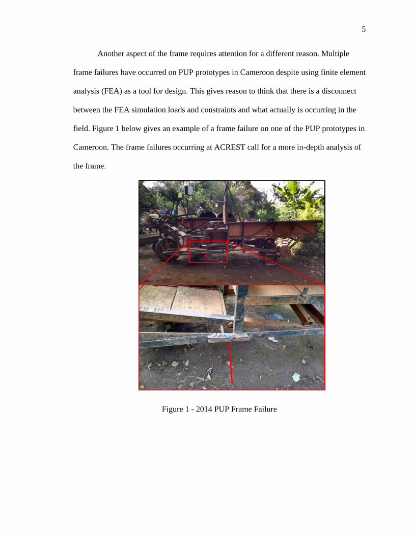
Another aspect of the frame requires attention for a different reason. Multiple

frame failures have occurred on PUP prototypes in Cameroon despite using finite element

analysis (FEA) as a tool for design. This gives reason to think that there is a disconnect

between the FEA simulation loads and constraints and what actually is occurring in the

field. Figure 1 below gives an example of a frame failure on one of the PUP prototypes in

Cameroon. The frame failures occurring at ACREST call for a more in-depth analysis of

the frame.

Figure 1 - 2014 PUP Frame Failure

6

6

1.5 Scope of Work

These failures in the field and the demand for a safe and reliable design for large

scale production have called for a more in-depth study of the PUP and its frame. In order

to assess the effectiveness of the FEA study, an experiment must be run on the frame of

an existing PUP to determine the actual stress in the frame. Once actual data on the frame

has been collected, then it can be correlated back to the FEA simulation. Developing a

method of collecting data on the PUP will, therefore, be essential. The remainder of this

paper goes into depth on the background research related to the PUP and the

methodology and results for assessing the stress in the frame and overall vehicle

dynamics. The conclusion of this work will help toward building a better PUP design that

can address sub-Saharan Africa’s transportation and agricultural needs for a more food

secure future.

7

7

CHAPTER 2. BACKGROUND RESEARCH

2.1 History of Agricultural Mechanization

History has shown that agricultural mechanization can boost farming yields

significantly in a relatively short period of time when the economic and technological

environment are agreeable. Agricultural mechanization has been defined by the Food and

Agriculture Organization of the United Nations (FAO) as the application of tools,

implements, or other powered machinery that are used as farming inputs to achieve

agricultural production. These agricultural machines are generally powered through

manual human power, animal power, or motorized power in application for land

development, crop production, harvesting, storage, processing, and transportation

(Houmy & Food and Agriculture Organization of the United Nations. Plant Production

and Protection, 2013). During the time period of 1880 to 1970, the United States (US)

saw a significant increase in agricultural production by mechanizing more operations.

Agricultural mechanization allowed for unused land to be developed to produce more

food. During this same time period, Japan and many European countries who had more

land constraints than the US also saw a significant increase in agricultural production.

They concentrated more on biological, yield-raising technologies, and later adapted more

mechanized solutions to increase production. This period of 90 years also marked an

increase in land/labor ratios for all of the mentioned countries, particularly after the

8

8

1950’s. This factor seems to have driven the demand for agricultural mechanization as

labor became more scarce with people moving into the more industrialized urban setting.

Additionally, the US land/labor ratio increased even faster with the increase in available

farm land and decrease of available labor. This shows that agricultural mechanization is

best suited for situations where land is abundant with little available labor (Binswanger-

Mkhize, 1984).

The Green Revolution marked another significant time in history where

agricultural production increased substantially throughout the world due to the

introduction of high yield plant varieties and new mechanized agricultural technologies.

In the 1940’s, Norman Borlaug developed a high-yield wheat variety that forever

changed Mexico’s food supply. By coupling this new wheat variety with mechanized

technologies, Mexico went from importing half of its wheat supply to becoming a wheat

exporter in approximately 20 years. This great success then spread to other regions of the

world (Briney, 2015). In the 1970’s, Asia began to see significant improvements in

agricultural production due to the Green Revolution. This success was attributed to the

large investments into motorized irrigation, fertilizer, high-yielding plant varieties, and

tractors. These key biological and mechanical technologies worked together to greatly

alleviate food insecure populations.

India’s crop production increased substantially during an intentional increase in

agricultural mechanization which began with the Green Revolution. From 1960 to 2010,

grain yield has increased steadily from 700 kg/ha to 1950 kg/ha. During this same time,

the number of irrigation pumps, fertilizer use, power tillers, and tractors all increased

dramatically in number in India. Irrigation pumps increased in number from 0.4 million

9

9

to 28 million. Fertilizer use increased from 2 kg/ha to 160 kg/ha. Power tillers increased

from 0 to 200 thousand. Tractors increased from 37 thousand to 4 million (Kienzle,

Ashburner, & Sims, 2013). India has provided an excellent example of how agricultural

mechanization can be applied to achieve higher agricultural outputs.

2.2 Agricultural Mechanization in Sub-Saharan Africa

Sub-Saharan Africa (SSA) is no stranger to the idea of agricultural mechanization.

During various times, governments in SSA have introduced different programs to

encourage farmers to use agricultural machinery, particularly tractors. Many of these

programs did not increase the adoption rate of mechanization and fell into financial and

operational problems (Houmy & FAO, 2013). Additionally, low land-labor ratios and

rural wages diminished demand for mechanization services (Benin, 2015). Tractors and

other agricultural equipment have been imported into countries in SSA only to fall into

disrepair due to an inadequate support system. Tractor owners cannot find replacement

parts when their equipment breaks down or needs standard maintenance. As a result,

imported farm tractors are abandoned at the beginning of their normal lifespan. More

sustainable designs and programs need to be introduced into this region to fully realize

the potential of this region.

In general, SSA lags behind in agricultural mechanization in comparison with

other developing regions of the world. A study was done where averages were taken

between 9 developing countries around the world for cereal yields, fertilizer use,

irrigation, and tractor use. It was found that these developing regions have 3.2 times

higher cereal yields, 16 times higher fertilizer use, 7.6 times higher irrigation percentage

10

10

of arable land, and 8.6 times higher tractors per 1000 ha than Africa as a whole excluding

Egypt and Mauritania (Houmy & FAO, 2013). SSA has not realized the benefits

mechanized power to help increase agricultural production, but that may change in the

future.

Although much of SSA has not seen productive results from successful

mechanization programs, some examples of success do exist. In Nigeria, it was found that

the real GDP in the agricultural sector grew 12.2% from 2000 to 2007 during a time of

intensified agricultural mechanization through tractor importation (Adelekan, 2012).

Also, a study in Ghana analyzed a credit facility called AMSEC that worked toward

making agricultural mechanization services available and affordable. Farmers provided

with credit were able to purchased tractors with implements and pay back the loan over a

period of 5 years. Later in 2011, a survey of 270 of these farmers was taken to determine

the effectiveness of the program. The majority of these farmers reported a reduction in

the drudgery aspect of farming (80% of farmers surveyed) and increased farming yields

(77% of farmers surveyed) (Benin, 2015). These pockets of success show potential for

mechanizing other parts of SSA.

Conditions similar to those in the United States, Europe, and Japan during the

significant increase in agricultural mechanization and production from 1880 to 1970 are

beginning to arise in SSA. People in the rural areas are beginning to move to urban

environments. Many rural workers are seeking off-farm employment while younger

generations who are tired of the drudgery aspect of working on a farm are moving to

cities. This is leading to a shortage in rural labor and is driving up the wages for hired

help while international food commodity prices also increase (Houmy & FAO, 2013).

11

11

The land/labor ratio is increasing in SSA making it easier for farmers to justify the capital

investment into mechanization of farming activities.

2.3 Benefits of Agricultural Mechanization

Agricultural mechanization has many benefits toward increasing a farmer’s

profitability and overall production. Many power intensive processes that require little

control like water pumping, threshing, maize grinding, and tilling are the first operations

to be mechanized on a farm. Also, transportation often is motorized to increase

production. Some of these mechanized solutions benefit a farmer’s production directly by

increasing yields through inputs like water, fertilizer, and seed. For example, motorized

water pumps can provide large amounts of water to crops relatively quickly and cheaply

in comparison to manual and animal powered methods (Binswanger-Mkhize, 1984). This

mechanized solution directly increases crop yields without displacing labor. Other

mechanized solutions like threshing and maize grinding generally indirectly increase

agricultural production by decreasing the time spent on those activities, so that the farmer

can spend his time on more productive activities. Some of those mechanized solutions

can also increase the value of the crops. A study done in Nigeria investigated how

farmers used tractors and how that use benefited them. They found that farms with

agricultural mechanization also used more intensive amounts of fertilizer, seed, and

chemicals and hired helped. Additionally, the correlation between tractor use and non-

farm income earners was much stronger than tractor use and crop sales in the North

region of Nigeria where farm sizes are relatively small (Takeshima, Min-Pratt, &

Xinshen, 2013). This study showed that agricultural mechanization has many effects both

12

12

on and off the farm. In some cases, it directly increases farm production and sales by

efficiently applying inputs like fertilizer and water. In other cases, it allows farmers more

time to seek additional non-farm income. For example, farmers may rent threshing units

to thresh their maize and greatly reduce the amount of time spent on that activity. This

time can now be used to work a side business selling SIM cards for cell phones in a local

market. In either case, farmers who may be in a subsistent lifestyle earn more income to

break the poverty cycle.

Smallholder farmers in particular can see the benefits of agricultural

mechanization by increasing the efficiency of farming operations, reducing harvest and

post-harvest losses, decreasing the drudgery aspect of farming, and creating a more

attractive environment for youth to engage in agriculture (Bishop-Sambrook, 2005).

Although the definition varies based on relative farm sizes in a region and overall

productivity of land, a smallholder farmer owns in the range of 1 to 10 hectares of land

(Dixon, Tanyeri-Abur, & Horst, 2004). Smallholder farmers comprise a large majority of

farmers in SSA and generally live in a state of subsistence where they can grow a

minimal amount of food for themselves and their family. Smallholder farmers in SSA

currently rely primarily on hand tool technologies (Houmy & FAO, 2013). Although

these farmers can benefit greatly from agricultural mechanization, it can be difficult for

them to adopt these devices primarily due to their cost. Smallholder farmers need

mechanized solutions that have low capital cost, multiple uses, and requires little to no

training to use. The capital cost can be a difficult obstacle to overcome. In many

countries, the private sector has established hire services for tractors and other

agricultural equipment for neighboring farms, generally small scale, who do not have

13

13

access to these tools (Houmy & FAO, 2013). The hire service provider earns more money

and pays off the capital investment for the equipment faster while the neighboring

smallholder farmer gains access to affordable agricultural mechanization.

2.4 Transportation in Sub-Saharan Africa

Transportation remains a serious challenge in SSA as few roads exist and what

roads that do exist are often not well maintained. Vehicles that use the roads often need to

be off-road capable to traverse certain rural areas. To further complicate the issue, few

cars and trucks exist in SSA in terms of the population. Table 1 summarizes data from the

World Bank showing the number of vehicles per 1000 people in several countries

throughout SSA.

14

14

Table 1 - Motor Vehicles Per 1000 People In Sub-Saharan Africa (ChartsBin, 2011)

Country

Name

Motor Vehicles

per 1000 people

Source

Year

Benin 21 2007

Botswana 113 2007

Burkina Faso 11 2008

Ethiopia 3 2007

Ghana 33 2007

Kenya 21 2007

Malawi 9 2007

Namibia 109 2007

Niger 5 2005

Nigeria 31 2007

Rwanda 4 2008

Senegal 23 2008

South Africa 159 2007

Tanzania 73 2007

Uganda 7 2008

Zambia 18 2007

Average 40

The number of available vehicles for people’s use varies considerably from country to

country, but averages to around 40 vehicles for a group of 1000 people. For perspective,

the United States had 809 vehicles per 1000 people in 2008 (ChartsBin, 2011). These

vehicles include passenger cars, buses, motor coaches, lorries, vans, and road tractors.

The lack of available transportation can be partially attributed to high importation costs

and inadequate vehicle support through replacement parts.

15

15

Current transportation methods in SSA are poor or costly and partly constrain

smallholder farmers to a life of subsistence living because of a lack of access to farming

inputs like fertilizer (Riverson & Carapetis, 1991). SSA relies primarily on manual

methods of transportation to move goods around. Smallholder farmers in particular rely

on transporting grain from their farms to local markets by carrying it manually, using a

bicycle, or by using animal-carts (Zorya, Morgan, Rios, Hodges, & Bennett, 2011). In

some cases, cars and trucks can be used or hired to transport grain over relatively large

distances, but this is often too costly. In East Africa, over 90% of transportation used to

move agricultural produce from the field to homes and local markets is done by carrying

it on the heads of women and children (Kienzle et al., 2013).

Transportation costs can become quite significant to farmers. One study done in

2008 showed that transportation costs for maize ranged from 64-84% of the total maize

marketing costs in the respective countries of Kenya, Uganda, and Tanzania. The same

study also reported 13% post-harvest losses due to poor road conditions (Zorya et al.,

2011). These financial losses reduce the incentive for farmers to grow more than

subsistent amounts of food to sell at local markets. These limited and high cost

transportation services lead to low mobility rates and market interactions which leads to

poor health and education outcomes leading to poverty (Hine, 2014). Furthermore, the

sparse amount of available transportation lead to increased costs for farm inputs (i.e.

seed, chemicals, and fertilizer), increased costs to access local markets, higher risk in

investing to produce a surplus of crops, and higher post-harvest losses due to spoilage

(Godfray et al., 2010). By addressing the transportation challenge in SSA, many farmers

16

16

living in subsistence may be able to save more of their money to apply towards moving

beyond poverty.

Although much of SSA does not possess large numbers of passenger vehicles and

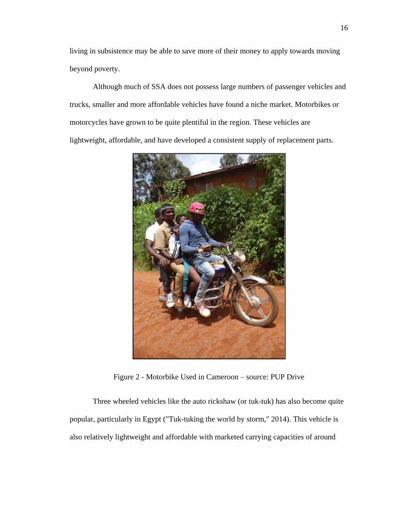
trucks, smaller and more affordable vehicles have found a niche market. Motorbikes or

motorcycles have grown to be quite plentiful in the region. These vehicles are

lightweight, affordable, and have developed a consistent supply of replacement parts.

Figure 2 - Motorbike Used in Cameroon – source: PUP Drive

Three wheeled vehicles like the auto rickshaw (or tuk-tuk) has also become quite

popular, particularly in Egypt ("Tuk-tuking the world by storm," 2014). This vehicle is

also relatively lightweight and affordable with marketed carrying capacities of around

17

17

500 kg (1102 lb) and max speeds up to 60 km/h (37.3 mph). These vehicles have diesel

engines with a net power of 5.7 kW (7.6 hp). For the most part, these vehicles are best

suited for urban settings.

Figure 3 - Auto Rickshaw or Tuk-Tuk (Lovson, 2016)

Similar to these three wheeled vehicles are Chinese trikes which are also

becoming more prevalent on the streets of SSA. These vehicles resemble a motorcycle

that has been attached to a cart and is advertised to carry payloads around 1000 kg (2205

lb) and has a top speed up to 80 km/h (50 mph). Motorcycle engines around 12 kW (16

hp) power the vehicle. Like the auto-rickshaw, these vehicles are found more in urban

settings.

Figure 4 - Kavaki Motor Chinese Trike ("Alibaba Manufacturer Directory - Suppliers,

Manufacturers, Exporters & Importers," 2016)

18

18

Two wheel walk behind tractors have also begun to enter the SSA rural market.

These pieces of agricultural equipment have multiple uses in the field by powering tillers,

water pumps, and a variety of other attachments. They can also be used as a mode of

transportation by pulling trailers or by installing a seat attachment. The two wheel tractor

pictured in figure 5 has an 8 kW engine (10.7 hp) and has a top speed of 19 km/h (12

mph).

Figure 5 - Two Wheel Multi-Function Tractor with Seat Attachment (Alibaba, 2016)

Motorbikes, auto rickshaws, Chinese trikes, and two wheel tractors each fill a role

in the SSA market, but they each have different advantages. Table 2, compiled by

Riverson and Carapetis, compares several different intermediate methods of

transportation ranging from manually powered wheelbarrows and bicycles up to the

Asian utility vehicle. No currency is quoted for the relative costs.

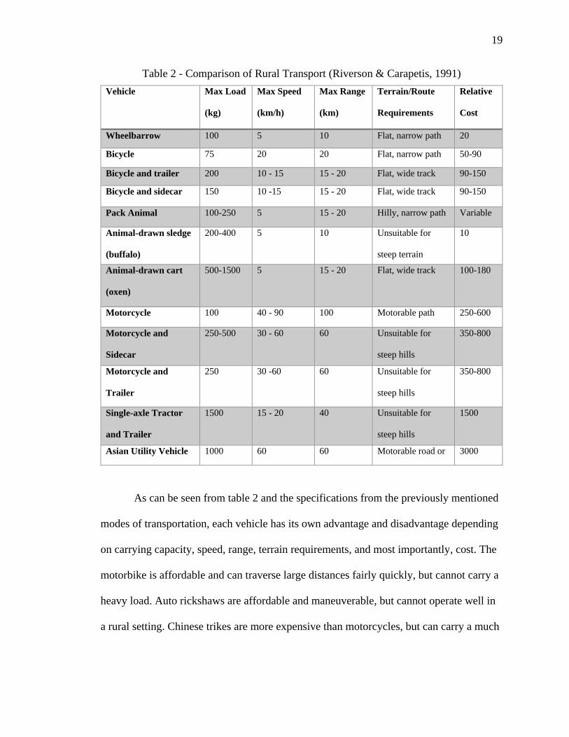
19

19

Table 2 - Comparison of Rural Transport (Riverson & Carapetis, 1991)

Vehicle Max Load

(kg)

Max Speed

(km/h)

Max Range

(km)

Terrain/Route

Requirements

Relative

Cost

Wheelbarrow 100 5 10 Flat, narrow path 20

Bicycle 75 20 20 Flat, narrow path 50-90

Bicycle and trailer 200 10 - 15 15 - 20 Flat, wide track 90-150

Bicycle and sidecar 150 10 -15 15 - 20 Flat, wide track 90-150

Pack Animal 100-250 5 15 - 20 Hilly, narrow path Variable

Animal-drawn sledge

(buffalo)

200-400 5 10 Unsuitable for

steep terrain

10

Animal-drawn cart

(oxen)

500-1500 5 15 - 20 Flat, wide track 100-180

Motorcycle 100 40 - 90 100 Motorable path 250-600

Motorcycle and

Sidecar

250-500 30 - 60 60 Unsuitable for

steep hills

350-800

Motorcycle and

Trailer

250 30 -60 60 Unsuitable for

steep hills

350-800

Single-axle Tractor

and Trailer

1500 15 - 20 40 Unsuitable for

steep hills

1500

Asian Utility Vehicle 1000 60 60 Motorable road or

track

3000

As can be seen from table 2 and the specifications from the previously mentioned

modes of transportation, each vehicle has its own advantage and disadvantage depending

on carrying capacity, speed, range, terrain requirements, and most importantly, cost. The

motorbike is affordable and can traverse large distances fairly quickly, but cannot carry a

heavy load. Auto rickshaws are affordable and maneuverable, but cannot operate well in

a rural setting. Chinese trikes are more expensive than motorcycles, but can carry a much

20

20

larger load on reasonable roads. Two wheel tractors are less suited for transportation, but

are relatively affordable, can pull a significant load, and has multiple uses outside of

transportation. Few vehicles exist that answer the need for affordable, durable, and off-

road capable transportation that can carry a significant load over a moderate distance.

Transportation is an important aspect of agricultural mechanization that provides

rural community members in SSA, particularly smallholder farmers, important access to

food, water, local markets, health care, farming inputs. Mechanized transportation helps

farmers both in transporting goods to markets and also carrying goods back from market.

This means that costs to move produce to markets decrease along with the costs of

bringing farming inputs back to the farm. A farmer benefits both ways. For some

smallholder farmers, fertilizer and high-yielding seed may be out of their reach due to the

large distances that must be traveled. Having any affordable method of transportation

could mean substantial yield increases. Several affordable modes of transportation exist,

but no affordable vehicle exists that can traverse the rural roads of SSA over long

distances while carrying large loads and providing multiple uses.

2.5 The Purdue Utility Platform

2.5.1 The Reason and Introduction for the Purdue Utility Platform

Sub-Saharan Africa plays a pivotal role in the fight against world hunger, and the

challenge of nearly doubling the food supply by 2050. Sustained agricultural

mechanization has increased agricultural production substantially in countries all over the

world. These mechanized solutions coupled with yield boosting farming inputs can bring

smallholder farmers in SSA out of subsistence and produce a surplus of food to feed the

21

21

world. Before this can happen though, technical solutions must be made that can be built

and implemented in sub-Saharan Africa that are sustainable and appropriate. When

approached by a non-governmental organization (NGO) about this challenge, Purdue

University began developing designs for a utility vehicle (later to be called the Purdue

Utility Platform or PUP) that addressed the need for affordable agricultural

mechanization in SSA. Particularly, this mechanized solution would address the needs for

affordable transportation while providing mechanical power to increase production on the

farm. The PUP itself is a low cost, locally maintainable, and off road capable three

wheeled utility vehicle that is capable of carrying around 900 kg, travel up to speeds of

30 km/h, and power an array of attachments and implements. Parts for the PUP can be

readily found in SSA by using existing supply chains and local raw materials. This

characteristic allows the PUP to function sustainably in rural environments.

2.5.2 The History of the Purdue Utility Platform

The research and design work for the Purdue Utility Platform (PUP) originally

began after the NGO known as the African Center for Renewable Energy and Sustainable

Technologies (ACREST) approached Purdue University with the challenge of developing

a sustainable vehicle for rural Cameroon. This NGO needed a more sustainable solution

for transportation to carry out daily activities around their local area. Their current

transportation options were costly and often needed repairs and replacement parts that

were not available. ACREST therefore worked with faculty and students at Purdue

towards developing a set of design constraints that needed to be followed to implement a

22

22

successful solution in the rural area. The main constraints were as follows (Lumkes,

2012):

1) Cost - The vehicle cost had to be kept as low as possible. A goal of $2000

USD was set to build the vehicle.

2) Easily Manufactured and Maintained - The vehicle build could only use

materials and tools that could be found locally in rural Cameroon.

3) Payload - The vehicle must carry a significant amount of payload. A goal was

set of carrying more than 600kg.

4) Reasonable Cargo Area – The cargo area must be greater than 2 m2.

5) Ergonomics – Inherently safe operation (stable, brakes, shields, etc.)

With these constraints set, Purdue University began an iterative approach to developing

this utility vehicle based on feedback from ACREST. Starting in 2009, the PUP project

became a senior design project for students to design, build, and test a prototype vehicle

at Purdue University before traveling to Cameroon to build a refined prototype there

using local materials. Valuable feedback from ACREST was used to improve the designs

and to implement new prototypes on an annual basis.

The PUP team developed the general framework for the vehicle after several

brainstorming sessions. The utility vehicle would have three wheels and a truss frame

made from local raw materials to keep the cost of the vehicle to a minimum. A three

wheel design is cheaper to build than a four wheel design, and a truss frame has the

advantage of being lightweight and strong. Less raw material is needed and thus reduces

the cost and keeps the weight of the vehicle lower so that a smaller, cheaper engine can

23

23

be used. To further lower the cost, the design of the vehicle only considered local

manufacturing techniques and materials. This would make the vehicle more affordable by

eliminating some importation costs and take advantage of the economies of scale of

existing supply chains. This design decision would also contribute to the constraint of

having the vehicle easily maintained.

The PUP has gone through 6 iterations since 2010 up to the present 2015 model.

Each iteration has taught many valuable lessons toward making a sustainable design that

can be implemented in rural SSA. The first PUP iteration incorporated a wooden frame,

belt driven CVT, 10 hp diesel engine, and a solid truck axle suspended by coil springs.

Figure 6 - 2010 PUP with Wooden Frame

This PUP in particular taught many lessons toward designing a sustainable vehicle in

rural Cameroon. The primary problems came from the transmission, frame, front steering

support, and vehicle dynamics. The belt driven CVT was not a sustainable transmission

24

24

as it could not be replaced or repaired. The wooden frame managed to withstand the road

loads, but made it difficult to mount the front strut due to the size of the wood. In order to

be strong enough, large pieces of wood need to be used as structural members, which

limits the number of wood members that can attach to the front strut. As a result, the front

strut was not well secured and ultimately failed. This utility vehicle also had a high center

of gravity (CG) which attributed to a high rollover potential. This vehicle lasted

approximately a month before being retired due to failures.

The 2011 PUP made significant improvements over the 2010 PUP. The design

used a frame comprised of steel tubing, an innovative manual belt transmission and

powertrain, a 10 hp diesel engine, a dumping bed, and an air spring attached to the rear

trailing arm for suspension. The CG for the vehicle was also lowered to reduce the

rollover potential.

25

25

Figure 7 - 2011 PUP in Cameroon

The truly innovative portion of this design came from its low cost and locally

manufactured transmission and powertrain. A series of V-Belts and levers were used to

create different gear ratios to power the rear wheels which functioned similarly to a rear

differential. The final vehicle specifications can be found in table 3.

Table 3 - 2011 PUP Specifications (Lumkes, 2012)

Capacity (kg) 600+

Speeds (km/h) 6, 13, 28 (depending on gear)

Build Cost (USD) $1800

Empty Mass (kg) 450 kg

26

26

Although innovative and a substantial improvement over the previous model, this design

was not without its own challenges. The major areas for improvement were as follows:

The engine overheated and was loud due to being enclosed directly behind the

driver.

The transmission and powertrain V-belt system was complex and required a

significant amount of time to assemble and fine tune.

The vehicle would not always reverse due to inadequate chain wrap on the

reversing gear.

The 2011 PUP functioned well in Cameroon, but further improvements were made.

Ultimately, this vehicle was used for parts for future PUP builds.

The 2012 PUP improved upon the previous PUP model in the areas of engine

cooling, powertrain, suspension system, bed space, and improved utility. The engine

cooling problem was addressed by mounting the engine on the front of the vehicle where

it could receive adequate air flow. During previous trips to Cameroon, it was found that

recycled car parts, primarily from Toyota Corolla’s, could be purchased and used in the

PUP design. A manual rear wheel drive transmission and differential, although slightly

more expensive than the V-belt system was easier to attach and more reliable. This PUP

iteration also implemented for the first time suspension on all of the wheels which

reduced stress on the frame and made the overall driving experience less taxing on the

driver. The frame itself now was comprised of mild steel angle iron and had a more box

shape to maximize the PUP’s bed space.

27

27

Figure 8 - 2012 PUP at ACREST in Cameroon

Also new to this model, attachments and implements like water pumps, maize grinders,

and planters were used to add additional utility to the vehicle and provide valuable

services to local farmers.

Figure 9 - Maize Grinder Attachment (Top Left), Water Pump Attachment (Top Right),

and Planter (Bottom)

28

28

The main areas of potential improvement for this vehicle were:

The car struts used for suspension provided for a rough ride due to the high spring

load. The struts were meant for a heavier vehicle and did not compress when the

PUP was not loaded.

The frame had fatigue failures after several weeks of use.

The CG could be lowered further to reduce the roll potential.

The 2013 PUP improved upon the previous year’s model by adopting a rear

trailing arm, lowering the CG, and by making frame changes to address failures. The rear

trailing arm added additional roll stiffness and softer suspension while removing the need

for problematic car struts which protruded into the bed of the vehicle. Removing the car

struts and using shorter coil springs also lowered the bed of the vehicle and therefore the

CG. The PUP driving experience greatly improved over the previous model under light

loads.

29

29


This model’s areas of improvement were as follows:

The trailing arm had angle iron failures.

The front strut would bottom out on the steering arm.

The CG could be lowered more to decrease the roll potential.

Engine placement made it easy to steal.

The 2014 PUP made significant improvements in lowering the CG of the vehicle

while modifying the powertrain to place the engine under the passenger seat. Also, the

rear trailing arm was shortened to reduce the amount of stress acting on it as the rear

wheels drove over rocks and potholes.

30

30

Figure 11 - 2014 PUP at Purdue

This vehicle experienced issues with the V-belt clutching system. The location of the

engine made it more complicated to tension and de-tension the V-belt that ran between

the engine and a countershaft. Several V-belt failures occurred. The areas of

improvement for this vehicle were:

The clutching system needed improved to address failures.

Frame failures where the front strut members tied into the frame.

Powertrain assembly was time consuming and required carefully aligning several

shafts.

The 2015 PUP improved upon the previous year by adopting an automotive clutching

system, making several modifications to the truss frame, and by improving the front

steering problem. These changes made the vehicle much more reliable and simpler to

31

31

manufacture. A power train tunnel was created within the frame of the vehicle to allow

for a larger variety of transmissions to be used.


Feedback on this prototype is still in the initial stages, but the original 2015 prototype had

several frame failures due to poor quality angle iron. A second prototype was built in

Cameroon to address these failures and has had no reported problems after several

months of being used regularly. The 2015 PUP has shown a great deal of promise and

now work is being done to scale this design.

32

32

2.5.3 Specifications for 2015 PUP

Table 4 - 2015 PUP Specifications

Empty Weight <500 kg

Payload 700-900 kg

Bed Dimensions 0.99 m wide x 1.90 m long

Transmission 5-speed + reverse (hi-low range option for 10 speeds)

Engine Any 4-8 kW small engine (typically diesel)

Length / Width 3.7 m / 1.45 m

Top speed 30 km/hr (configurable)

Brakes Hydraulic brakes on each wheel

Suspension Coil springs on each wheel – torsion bar for high roll stiffness

Frame Lightweight truss – 35 x 35 x 3.5 mm angle iron

Building Cost $1,200-$2,000 USD (excludes labor and licensing costs)

Figure 13 – 2015 PUP Dimensions

33

33

2.5.4 Technical Lessons Learned

Two consistent concerns have been at the forefront of the work done on the PUP

throughout its history: frame failures and the potential to roll the vehicle. Each of these

areas must be considered before scaling this vehicle design. Despite using engineering

tools like finite element analysis (FEA) to determine areas of high stress, the frame

continues to have unforeseen failures. Also, little work has been done to determine the

roll stability of this vehicle. Nearly every iteration lowered the CG of the vehicle to make

it safer, but the actual conditions for rolling are not fully explored.

2.6 Truss Frame Research

2.6.1 Truss Frame Fundamentals

A truss frame is a specially designed structure made from straight members that

are joined in such a way that they do not transmit bending (Case, Chilver, & Ross, 1999).

The traditional construction of a truss can be seen in figure 14. Triangular structures

make up the composition of any truss frame. These triangular pieces make a structure

rigid and ensures that loads acting at the joints of the structure (ex. point “b” in figure 14)

only cause the members to compress or stretch without bending. Each node or

intersection of straight members can be considered a ball joint. If members BC, CE, and

DE were removed from the truss structure in figure 14, then a box would form. This box

would have ball joints in each corner and would no longer be a rigid structure. It would

sway back and forth. Adding in the diagonal members will triangulate the structure and

make it rigid again. This helps conceptualize how the members do not bend (like in the

case of the square), but only are subject to tension and compression. This unique

34

34

characteristic allows truss frames to be lightweight yet strong. This characteristic has

found many applications in the engineering world.

Figure 14 - Simple Truss (Connor & Faraji, 2012)

2.6.2 Types of Trusses and Applications

Truss frames can be found in a variety of structures and applications. To begin,

several truss types have been used in the construction of bridges, towers, domes, roofs,

and other buildings. One icon example is the Eiffel tower (Connor & Faraji, 2012).

Figure 15 - Types of Truss Shapes (Connor & Faraji, 2012)

35

35

The lightweight and strong construction of a truss frame has also particular application in

aeronautics. These same planar truss shapes used in building bridges has also been used

in building airplane fuselages. For example, the Warren truss is used in some applications

for fuselages for light, single engine airplanes (United States. Flight Standards, Aviation,

amp, & Academics, 2012).

Figure 16 - Warren Type Airplane Fuselage (United States. Flight Standards et al., 2012)

The automotive industry has also benefited from using truss structures known as

space frames. High performance cars have specifically taken advantage of the high

weight/power ratios that can be achieved by using lightweight yet strong space frames.

Since the 1960’s, race cars have used space frames for their light weight construction,

high torsional stiffness, and strong safety structures for rolling and crashing (de Oliveira

& Borges, 2008). For example, the Jaguar C – Type was one of the first cars to utilize a

space frame. This can be seen in figure 17.

36

36

Figure 17 - Jaguar C – Type with Space Frame (Classics, 2016)

2.6.3 Analysis of Space Frames

Much work has been done towards developing methods to decipher the structural

integrity of a vehicle’s frame. In many cases, a finite element analysis (FEA) tool like

ANSYS is used as a design tool. Significant amounts of time and money can be saved by

using FEA to calculate the general stresses acting upon a vehicle’s chassis by eliminating

the need to build and test a prototype (Jain, 2014). One frame study employed the general

process of correlating test data to a simplified FEA model in order to determine the loads

acting on the frame. The loads were then used in a FEA and fatigue study for a new

frame (Wen, 2008). Another study on a motorcycle frame used experimental data

collected from strain gauges to calculate the loads acting on the frame through a matrix

inversion method (Hirai, Ueno, Iwaki, & Oohama, 2013). Optimization modules are also

used to find the lightest possible frame while keeping an optimal strength (Wen, 2008),

(Johnson, 1986). Several frame studies use a combination of FEA and experimental data

from strain gauges to determine the real loads acting on the frame in order to develop a

model that optimizes the strength and weight of the vehicle.

37

37

Formula-SAE and Baja vehicle teams both take advantage of using FEA and

experimental data to find the optimal solution for their space frames chassis. Although

the general process of validating an FEA model exists, it can be a difficult process to

follow. “While the process of solving Finite Element problems is a science, creating

models is quite an art” (Jain, 2014). In many cases, matching up an FEA model with an

actual experiment can be difficult due to the numerous variables that may be involved

such as the number of elements used and boundary conditions. Despite the difficulty,

progress has been made. Experiments run on Formula-SAE cars have shown that parts

(i.e. one corner of the vehicle) need to be able to withstand accelerations of 3.5g’s for

bumps, 1.5g’s for braking, and 1.5g’s for lateral accelerations (Riley & George, 2002).

Space frames like those for Formula-SAE cars experience the greatest loads due to

torsion loads from an uneven road surface or cornering forces. To determine if a frame

can withstand the necessary torsion loads, an FEA simulation similar to the one shown in

figure 18 can be used where the rear of the frame is fixed by four nodes (shown by red

triangles) and the front of the frame has two equal but opposite forces acting on it. The

stiffness of the frame can then be calculated based on the torque applied and the angular

deflection (Riley & George, 2002).

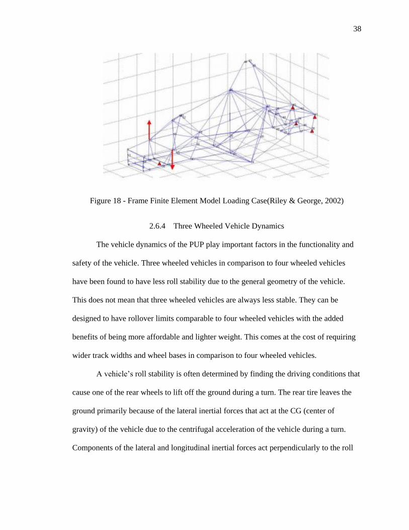
38

38

Figure 18 - Frame Finite Element Model Loading Case(Riley & George, 2002)

2.6.4 Three Wheeled Vehicle Dynamics

The vehicle dynamics of the PUP play important factors in the functionality and

safety of the vehicle. Three wheeled vehicles in comparison to four wheeled vehicles

have been found to have less roll stability due to the general geometry of the vehicle.

This does not mean that three wheeled vehicles are always less stable. They can be

designed to have rollover limits comparable to four wheeled vehicles with the added

benefits of being more affordable and lighter weight. This comes at the cost of requiring

wider track widths and wheel bases in comparison to four wheeled vehicles.

A vehicle’s roll stability is often determined by finding the driving conditions that

cause one of the rear wheels to lift off the ground during a turn. The rear tire leaves the

ground primarily because of the lateral inertial forces that act at the CG (center of

gravity) of the vehicle due to the centrifugal acceleration of the vehicle during a turn.

Components of the lateral and longitudinal inertial forces act perpendicularly to the roll

39

39

axis (line from the front tire contact patch to rear tire contact patch) of the vehicle and

cause the vehicle body to rotate around that axis. The result is that the vehicle rolls. The

weight of the vehicle is the only force that counter acts the inertial forces. This can be

seen in figure 19.

Figure 19 - Four Wheeled vs Three Wheeled Roll Dynamics

A vehicle design can be made safe by moving the CG to a location that decreases

the moment around the roll axis due to the inertial forces and increasing the moment due

40

40

to the weight of the vehicle. In other words, the CG height should be kept as low as

possible while the perpendicular distance from the roll axis to the CG (viewed from the

top of the vehicle) should be made as large as possible.

Three wheeled vehicles can be designed to operate safely within normal vehicle

operation by adjusting key characteristics of the vehicle including: track width, center of

gravity (CG) location, and suspension stiffness and damping. Increasing the track width

has a direct correlation of increasing the vehicle’s rolling stability by decreasing the

overturning moment (Raman, Rao, & Kale, 1995). Increasing the track width also

increases the perpendicular distance from the CG to the roll axis.

Apart from increasing the track width, roll stability can also be increased by

adjusting the location of the CG. Increasing the height of the CG makes a vehicle more

prone to rollover (Raman et al., 1995). As a general rule, the CG height should be kept as

low as possible to prevent rollovers. The roll stability also depends on the location of the

CG with respect to the front and back of the vehicle. For steady state turning, a three

wheeled vehicle’s roll stability increases as the CG moves toward the axle with two

wheels (Huston, Graves, & Johnson, 1982).

The suspension characteristics of the vehicle also determine how likely a vehicle

is to roll over. High spring rates or stiffer suspensions increase the roll stability of a

vehicle. This comes at a cost though. More stress is introduced into the frame and driver

comfort is sacrificed as the vehicle drives over disturbances in the road like potholes. An

optimal spring rate exists to find the balance between roll stability, frame integrity, and

driver comfort. Apart from spring rate, increasing suspension damping also increases

rolling stability by damping out oscillations.

41

41

Several general guidelines exist for designing a three wheeled vehicle with one

wheel in the front. One regulation for three wheeled vehicles in Canada (standard 505 in

Motor Vehicle Safety Regulations) requires that the CG height be less than 1.5 times the

horizontal distance from the CG to the nearest roll axis (Canada, modified:2016-04-07).

Other useful tools that can be used for three wheel vehicle design utilize equations that

were derived by finding the lateral acceleration that cause a wheel to lift off the ground

during a steady state turn. Equation 1 gives the lateral acceleration condition that will

cause a vehicle to overturn in a steady state turn excluding braking or accelerating (Van

Valkenburgh, Klein, & Kanianthra, 1982). The symbol g is the gravity constant.

𝑎𝑦

𝑔=

𝑇

2𝐿

𝑎

ℎ Equation 1

Figure 20 – Three Wheel Vehicle Symbol Explanation

42

42

CHAPTER 3. FRAME STUDY AND VEHICLE DYNAMICS METHODS

3.1 Introduction to Methodology

The assessment and optimization of the PUP has been a multi-step process. The

general process began with the development of the 2015 prototype which built on

previous experience from Cameroon and utilized Solidworks and ANSYS. Next, a

methodology was developed to collect a variety of data to further improve the design and

provide a measure of vehicle effectiveness. Finally, a FEA (Finite Element Analysis) and

roll stability simulation utilized collected information to provide a measure of predicted

vehicle performance. Overall, the methodology for the study on the PUP can be broken

down into the development of the 2015 PUP frame design, the vehicle data acquisition,

the validation of the FEA model, and the development of a roll stability simulation.

3.2 Vehicle Frame Design Improvements

The frame design for the 2015 PUP included a variety of changes meant to

improve the ease of manufacturability, vehicle reliability, and address the frame failures

seen in Cameroon. The main change that directed the 2015 frame design centered on the

idea of implementing a large power train tunnel that could house a variety of

transmissions and make room for the implementation of an automotive clutch. Consistent

v-belt failures determined the need for a more reliable automotive clutch since v-belts

43

43

comprised the main element in previous PUP clutching mechanisms. The powertrain

tunnel (see figure 21) resized the whole front half of the vehicle and made it possible to

put the engine, clutch, and transmission all into a line. This removed the need for an

additional counter shaft which the 2014 model implemented and greatly increased the

ease of assembly. Several other frame changes were made to make improvements

including a change to allow more ground clearance where the swing arm attaches to the

frame (figure 22). Experience had shown that collisions had occurred on this part of the

frame (figure 23). Crossing two front members on the front of the vehicle allowed the

engine to sit lower and reduce the vehicle CG height.

Figure 21 - Powertrain Tunnel

44

44

Figure 22 - Functionality Frame Changes

Figure 23 - 2014 PUP Frame Failure on Front Strut Lateral Member

Once the overall frame configuration had been developed, additional diagonal

members helped strengthen the frame. These were placed based on failures seen in

Cameroon (figures 24-25) and results from FEA software (ANSYS). The frame

strengthening additions can be seen in figure 26.

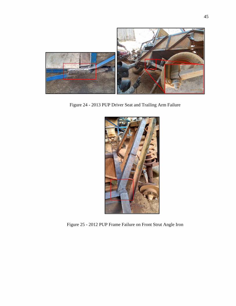
45

45

Figure 24 - 2013 PUP Driver Seat and Trailing Arm Failure

Figure 25 - 2012 PUP Frame Failure on Front Strut Angle Iron

46

46

Figure 26 - Frame Strengthening Additions

The FEA model developed in ANSYS used the geometry from Solidworks and

considered a combined loading scenario to produce the maximum possible stresses in the

frame. Loads were based off of known weights of components on the vehicle and

generalized lateral and longitudinal tire forces. Specifically, a 2000 lb load was applied

uniformly to the bed of the vehicle along with loads on the mounting brackets for the

transmission and engine weight. The simulation also considered loads from passenger

weight on the front seats and braking and lateral forces on the rear bearings and front

strut member. This produced simulation results like figure 27.

47

47

Figure 27 - ANSYS Solution for Combined Loading

3.3 Vehicle Data Acquisition

3.3.1 Importance of Data Acquisition

Data is important for assessing vehicle impact and improving the design. Data can

help answer questions like: What is the usage pattern on the vehicle? How long will the

vehicle last without major maintenance? How durable is the vehicle? Under what

conditions will the vehicle roll? These questions cannot always be directly and simply

answered. They can at least be addressed by collecting information through a variety of

methods. GPS data collected during the PUP’s operation could be used to ascertain its

impact in sub-Saharan Africa by determining when, where, and how often the vehicle is

used. Recording engine speed during vehicle operation could lend new insight into how

much power the PUP actually delivers to its operators. Strain gauge information could be

used to ascertain the longevity of the vehicle’s frame life and durability. Recording static

48

48

weights from individual tires on the vehicle could help determine the overall rollover

stability. All of these different types of data provide valuable insight and guidance for

future PUP designs.

Collecting data requires a data acquisition (DAQ) system with the capabilities

necessary to record data at appropriate speeds and accuracy. The PUP requires a mobile

system that could be attached to the vehicle and operate in adverse conditions. A basic

DAQ system would consist of sensors, data acquisition hardware, signal processing

software, and a storage device. This system could provide valuable information for

design work and could also be applied in an entrepreneurial sense. Transportation

businesses could use GPS data to keep track of all of their PUP’s in real time to ensure

timely delivery and assist when a driver has a problem. Developing different DAQ

systems for the PUP has a multitude of benefits.

3.3.2 Applications of a PUP DAQ System

Work on a DAQ system for the PUP began by researching an affordable means of

collecting information on the PUP that could be implemented in sub-Saharan Africa. To

answer this challenge, a small, generic microcontroller comparable to an Arduino Uno

was used in conjunction with a blue tooth antenna, cellphone, custom strain gauge bridge

and filter, and a custom android application to upload engine speed, engine temperature,

vehicle speed, and vehicle location to a Google Drive account (Corona, 2015). This DAQ

system was installed onto the 2015 PUP in water proof electrical boxes and was tested

while the vehicle operated in rainy conditions.

49

49

Figure 28 - Red Board DAQ System

This system operated well in inclement weather and proved to be an excellent system for

recording vehicle location and motion, but needed further refinement in order to record

engine speed, temperature, and frame stress.

A more streamlined DAQ system simply consisted of a GPS unit wired into the

switch of the PUP’s engine. Once the key turned, the GSM/GPRS/GPS Vehicle Tracker

TK103A would turn on and GPS coordinates would be stored to an SD card on the GPS

device and sent through a cell phone provider to a server that could be accessed online.

Figure 29 provides an example of an experiment run at Purdue displaying the collected

GPS data (blue line) in Google Earth.

50

50

Figure 29 - GPS Data Collected With TK103A Vehicle Tracker

3.3.3 Data Acquisition for Measuring Frame Stress and Validating FEA Models

The analysis of the PUP frame required a DAQ system that was mobile, had high

resolution, and an adequate sampling rate to measure stresses induced into the frame by

wheel displacements. The National Instruments (NI) 9219 coupled with the NI cDAQ-

9171 provided the necessary capabilities to adequately record information from strain

gauges and relay it to a laptop to be processed with LabVIEW. The drivers for the NI

9219 integrated well with LabVIEW in order to create a simple LabVIEW file that

allowed for relatively easy calibration. The LabVIEW wiring diagram of the .vi file

developed for this experiment can be found in the appendix. This DAQ system has four

independent channels each with a resolution of 24 bits and a sampling rate of 100 Hz and

can be powered by a laptop. This system mounted to the bed of the PUP in a plastic

container and connected to a Wheatstone near the strain gauges on the frame. The length

of the leads going from the strain gauge to the bridge were kept short to eliminate the

concern for the lead wire resistance from offsetting the strain readings. Micro-

51

51

Measurements EA-06-250TA-120 precision strain gauges with a gauge factor of 2.01

were used to sense strain and can be seen in figure 30.

Figure 30 - A Precision Strain Gauge Mounted To One of the Front Strut Angle Iron

Members

The DAQ system collected the signal from the strain gauges and calculated the

strain based on bridge configuration, excitation voltage, Poisson ratio, and gauge

resistance. A half bridge type 1 configuration was used to find strain and has the

characteristics of being able to measure axial and bending stress, is temperature

compensated, and compensates for aggregate effect on principle strain measurements due

to the Poisson effect (Instruments, 2016).

The truss configuration of the frame members on the PUP only allow axial stress,

so a half bridge configuration is able to accurately measure the stresses occurring while

52

52

being temperature compensated. A variety of Rosette strain gauges would also work in

this situation. Although they are expensive, they can be used when the direction of the

principal stress is unknown. Figure 31 depicts the half bridge type 1 configuration where

R4 is the active strain gauge and R3 is the strain gauge mounted transverse to the load.

R1 and R2 in the circuit diagram below are the bridge resistors and their resistance equals

the nominal resistance of the strain gauges.

Figure 31 – Half Bridge Configuration Type 1(Instruments, 2016)

Equations 2 and 3 describe the resulting measured strain for a type 1 half bridge

configuration (Instruments, 2016).

𝑠𝑡𝑟𝑎𝑖𝑛 (휀) = −4𝑉𝑟

𝐺𝐹[(1+𝑣)−2𝑉𝑟(𝑣−1)]× (1 +

𝑅𝐿

𝑅𝐺) Equation 2

𝑉𝑟 =𝑉𝑜

𝑉𝐸𝑋 Equation 3

𝐺𝐹 = 𝑔𝑎𝑢𝑔𝑒 𝑓𝑎𝑐𝑡𝑜𝑟

𝑣 = 𝑝𝑜𝑖𝑠𝑠𝑜𝑛 𝑟𝑎𝑡𝑖𝑜

𝑉𝑜 = 𝑚𝑒𝑎𝑠𝑢𝑟𝑒 𝑠𝑖𝑔𝑛𝑎𝑙 𝑜𝑢𝑡𝑝𝑢𝑡 𝑓𝑟𝑜𝑚 𝑠𝑡𝑟𝑎𝑖𝑛 𝑔𝑎𝑢𝑔𝑒

53

53

𝑉𝐸𝑋 = 𝑒𝑥𝑐𝑖𝑡𝑎𝑡𝑖𝑜𝑛 𝑣𝑜𝑙𝑡𝑎𝑔𝑒 (𝑉)

𝑅𝐿 = 𝐿𝑒𝑎𝑑 𝑟𝑒𝑠𝑖𝑠𝑡𝑎𝑛𝑐𝑒 (𝛺)

𝑅𝐺 = 𝑁𝑜𝑚𝑖𝑛𝑎𝑙 𝐺𝑎𝑢𝑔𝑒 𝑅𝑒𝑠𝑖𝑠𝑡𝑎𝑛𝑐𝑒 (𝛺)

Figures 32 and 33 depict the front panel and the data acquisition helper used to calibrate

the system. An elastic modulus of 200 GPa was assumed for calculating the stress from

collected strain values.

Figure 32 - Front Panel of Strain Gauge vi File

54

54

Figure 33 – Data Acquisition Helper

Strain gauge data can be difficult to decipher once it has been collected as the

knowledge of what happened at that point in time can be forgotten or not noticed.

Collecting video footage while recording data has many advantages and was a key

component in performing the frame analysis. Certain events like turning on the PUP

engine or hitting a large bump became markers for both the video and the strain gauge

data and allowed them to be synced together. Figure 34 shows the mounting of the

camera and an example video that has integrated GPS data. This allowed the vehicle

speed to be roughly calculated during wheel collision and braking tests.

55

55

Figure 34 –Video of Strain Gauge Experiment (left) Camera and Wheatstone Bridge

Mounting (right)

Once the DAQ system had been installed and calibrated through LabVIEW, the

validation of the FEA model began. Specific regions on the PUP frame were studied in

order to validiate the FEA model and determine the loads coming into the frame from the

wheels. The strain gauge locations can be found in figure 35. Three locations on the front

strut members were chosen in order to record stresses from front wheel collisions and

also stresses induced while braking. Frame failures in these members had occurred in

Cameroon which proved that these were high stress regions. Additionally, five locations

were chosen on the rear of the vehicle to record stress from the rear wheels due to wheel

collisons, wheel braking, and bed loads. The right trailing arm location is not shown in

figure 35.

56

56

Figure 35 - Strain Gauge Placement

57

57

Testing of the frame began once the DAQ system and strain gauges had been

installed in specific regions where relatively high stress was predicted to use for FEA

model development. The PUP underwent a series of driving tests including bump tests

and braking tests. These tests needed to be repeatable in order to draw reliable

conclusions. For the bump test, concrete parking stops with dimensions roughly 8.75”

wide and 4.625” tall were used due to their uniform size and availablility. The PUP drove

over 8 of these stops for several laps in a parking lot while in first gear traveling

approximately 4 mph while recording data onto a laptop in the bed of the PUP. The brake

test consisted of driving the PUP to its maximum speed on a straight gravel road and then

pressing the clutch and brake to decelerate the vehicle as quickly as possible. A water tote

provided additonal weight in the bed of the vehicle to test different PUP loading

configurations (see figure 35). The bump and brake tests were performed for both loaded

and unloaded PUP configurations.

3.4 FEA Model Study

The process for developing a simple static structural model in ANSYS that

corresponds with strain gauge data can be a difficult process. In many cases, complex

Multiphysics models are needed in order to take into account the inertial effects of the

mass of the vehicle, cargo, and passengers. Additionally, the wheel suspension integrated

with the suspended mass adds a degree of complexity that the ANSYS model does not

take into account. The static structural models used specific boundary conditions and

loadings to best represent the experimental work. These models used geometries from

58

58

Solidworks assembly files which were imported into ANSYS. Two simplified FEA

models represented the PUP during wheel collisions.

The first simplified ANSYS model concentrated only on the rear trailing arm of

the PUP. Studying only this part of the PUP allowed for faster simulation run times while

providing accurate results. The simulation considered two scenarios where the two rear

wheels hit a concrete parking stop at the same time and when only one rear wheel hit a

parking stop. Different boundary conditions needed to be considered for each of these

cases. For the wheels hitting the parking stop at the same time, the trailing arm was

allowed to rotate around the pins that insert into bearings but was also constrained

vertically where the suspensions springs connected with the trailing arm. Loads acted on

the wheels of the axle at 0 degree angles to represent the concrete stops colliding with the

wheels and springs absorbing the vertical forces. The trailing arm should not see any

stress from the vertical forces since the suspension springs absorb this force. Only

longitudinal forces are considered. The loads were then varied until the principle Von

Mises stress from the simulation matched the recorded values from the experiment. These

force loads were then correlated with a constant vertical acceleration based on the static

weight on the rear wheels and assuming the concrete stop hit the wheels at a 45 degree

angle. The scenario considering only one wheel collision had similar boundary conditions

as the previous scenario with the only change being that one side of the trailing arm was

allowed a displacement. A load was then only applied at a 45 degree angle to the wheel

that is free to move in the vertical direction. The newly discovered vertical accelerations

can be used with the static mass that is supported by each tire to determine the upward

force that hits each tire. The corresponding longitudinal force can then be found by

59

59

assuming a 45 degree impact, so the longitudinal force will equal the upward force. These

force components can then be used in future FEA models.

Figure 36 – ANSYS Static Structural Model Considering a Two Wheel Collision

The second simplified static structural ANSYS model only considered the main

frame of the PUP excluding the trailing arm. This model had boundary conditions at the

rear pillow block bearings, spring cups, and front strut bracket. The frame could not

move vertically at the rear spring cups (zero displacement vertically), and it could not

move longitudinally or laterally at the pillow blocks (zero displacement longitudinally

and laterally). These boundary conditions represented the coil springs and trailing arm

which were not included in the model. The angle of the strut was measured on the actual

vehicle and modeled in the static structural model in ANSYS. A force was then applied

equally to the front strut bracket pointing perpendicular to the surface where the strut

tower attached. This represented the force entering the front strut members due to the

60

60

front coil spring displacement. This model assumes that the longitudinal and lateral

forces are taken on by the strut members at the base of the wheel. Similarly as before, the

strut force found from the simulation to produce similar frame stress as in the

experiments is correlated to a constant acceleration based on the static weight on the front

wheel.

3.5 Rolling Stability Simulation

Three wheeled vehicles can be more prone to roll over in comparison to four

wheeled vehicles due to their geometry. In general, high CG heights and narrow track

widths lead to vehicle overturns. In the case of a three wheeled vehicle with a single

steered wheel in the front, braking while turning downhill decreases the rolling stability

of the vehicle. Three wheeled vehicles can be designed to be as stable as four wheeled

vehicles, but requires specific attention to the CG location of the vehicle and the overall

vehicle geometry. The PUP’s design accounted for the importance of keeping the

vehicle’s CG as low as possible and as close to the rear axle as possible, but the overall

rolling stability of the vehicle is largely untested. Knowing the roll stability of the vehicle

is important for people’s safety and must be considered. Rather than trying to roll an

actual running vehicle, a roll stability simulation has the benefit of being inexpensive,

safe, and easy to perform repeatedly.

The methodology behind developing a roll stability simulation for three wheeled

vehicles began by trying to consider a model that could be simple yet useful. Too

complex of a model would become too specific and require values of parameters that

would be difficult and time consuming to find. Too simple of a model would not be

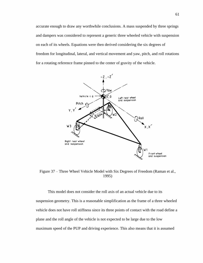
61

61

accurate enough to draw any worthwhile conclusions. A mass suspended by three springs

and dampers was considered to represent a generic three wheeled vehicle with suspension

on each of its wheels. Equations were then derived considering the six degrees of

freedom for longitudinal, lateral, and vertical movement and yaw, pitch, and roll rotations

for a rotating reference frame pinned to the center of gravity of the vehicle.

Figure 37 – Three Wheel Vehicle Model with Six Degrees of Freedom (Raman et al.,

1995)

This model does not consider the roll axis of an actual vehicle due to its

suspension geometry. This is a reasonable simplification as the frame of a three wheeled

vehicle does not have roll stiffness since its three points of contact with the road define a

plane and the roll angle of the vehicle is not expected to be large due to the low

maximum speed of the PUP and driving experience. This also means that it is assumed

62

62

the CG location does not change significantly due to the roll of the vehicle. This will be

verified based on simulated roll angles. The PUP does have a rear trailing arm that gives

the vehicle a certain amount of roll stiffness, so the actual suspended body will not roll as

much as the simulated vehicle.

The following principle equations (eqns. 4-9) were used for this simulation. It was

assumed that the vehicle body is symmetrical about the x-z plane down the center of the

vehicle which eliminates the cross products of Ixy and Iyz. Also, the body centered frame

coincides with the principle axes which sets all of the products of inertia equal to zero

(Gawade, Mukherjee, & Mohan, 2005). Aerodynamic forces are not considered in this

model as the PUP does not reach fast enough velocities for these forces to come into

play.

𝑚(𝑎𝑥) = 𝑚(�̈� + �̇��̇� − �̇��̇�) = 𝐹1𝑥 + 𝐹2𝑥 + 𝐹3𝑥 Equation 4

𝑚(𝑎𝑦) = 𝑚(�̈� + �̇��̇� − �̇��̇�) = 𝐹1𝑦 + 𝐹2𝑦 + 𝐹3𝑦 Equation 5

𝑚(𝑎𝑧) = 𝑚(�̈� + �̇��̇� − �̇��̇�) = 𝑚𝑔 − 𝐹1𝑧 − 𝐹2𝑧 − 𝐹3𝑧 Equation 6

𝑀𝑥 = 𝐼𝑋�̈� − (𝐼𝑦 − 𝐼𝑧)�̇��̇� = (𝐹2𝑧 − 𝐹3𝑧)𝑏 − (𝐹1𝑦 + 𝐹2𝑦 + 𝐹3𝑦)(ℎ − 𝑧) Equation 7

𝑀𝑦 = 𝐼𝑦�̈� − (𝐼𝑧 − 𝐼𝑥)�̇��̇� = 𝐹1𝑧𝐿𝑓 − (𝐹2𝑧 + 𝐹3𝑧)𝐿𝑟 + (𝐹1𝑥 + 𝐹2𝑥 + 𝐹3𝑥)(ℎ − 𝑧)

Equation 8

𝑀𝑧 = 𝐼𝑧�̈� − (𝐼𝑥 − 𝐼𝑦)�̇��̇� = 𝐹1𝑦𝐿𝑓 − (𝐹2𝑦 + 𝐹3𝑦)𝐿𝑟 + (𝐹2𝑥 − 𝐹3𝑥)𝑏 Equation 9

Equations 4-9 were rearranged into equations 10-15 and solved for using a

MATLAB script with integrated functions that utilized ode45 to solve the differential

63

63

equations. Equations 10-36 were used in a MATLAB function that ode45 called to solve

the differential equations given a set of initial conditions and a time interval.

�̈� =𝐹1𝑥+𝐹2𝑥+𝐹3𝑥

𝑚+ �̇��̇� − �̇��̇� Equation 10

�̈� =𝐹1𝑦+𝐹2𝑦+𝐹3𝑦

𝑚+ �̇��̇� − �̇��̇� Equation 11

�̈� = 𝑔 −𝐹1𝑧+𝐹2𝑧+𝐹3𝑧

𝑚+ �̇��̇� − �̇��̇� Equation 12

�̈� =𝑏

𝐼𝑋(𝐹2𝑧 − 𝐹3𝑧) −

(ℎ−𝑧)

𝐼𝑋(𝐹1𝑦 + 𝐹2𝑦 + 𝐹3𝑦) +

(𝐼𝑦−𝐼𝑧)

𝐼𝑋�̇��̇� Equation 13

�̈� =𝐿𝑓

𝐼𝑦𝐹1𝑧 −

𝐿𝑟

𝐼𝑦(𝐹2𝑧 + 𝐹3𝑧) +

(ℎ−𝑧)

𝐼𝑦(𝐹1𝑥 + 𝐹2𝑥 + 𝐹3𝑥) +

(𝐼𝑧−𝐼𝑥)

𝐼𝑦�̇��̇�

Equation 14

�̈� =𝐿𝑓

𝐼𝑧𝐹1𝑦 −

𝐿𝑟

𝐼𝑧(𝐹2𝑦 + 𝐹3𝑦) +

𝑏

𝐼𝑧(𝐹2𝑥 − 𝐹3𝑥) +

(𝐼𝑥−𝐼𝑦)

𝐼𝑧�̇��̇� Equation 15

𝐹1𝑥 = (𝑃𝑏𝑟𝑎𝑘𝑒

�̇�− 𝑓𝐹1𝑧) cos 𝛿 − 𝐹1𝑦 sin 𝛿 Equation 16

𝐹2𝑥 =𝑃

2�̇�− 𝑓𝐹2𝑧 Equation 17

𝐹3𝑥 =𝑃

2�̇�− 𝑓𝐹3𝑧 Equation 18

𝛼1 = tan−1 (�̇�+𝐿𝑓�̇�

�̇�) − 𝛿 Equation 19

𝛼2 = tan−1 (�̇�−𝐿𝑟�̇�

�̇�+𝑏𝜓) Equation 20

𝛼3 = tan−1 (�̇�−𝐿𝑟�̇�

�̇�−𝑏𝜓) Equation 21

𝐹1𝑦 = 𝐹𝑚𝑎𝑔𝑖𝑐 𝑓𝑜𝑟𝑚𝑢𝑙𝑎(𝛼1, 𝐹1𝑧 , 𝐶1, 𝜇𝑝) cos 𝛿 + (𝑃𝑏𝑟𝑎𝑘𝑒

�̇�− 𝑓𝐹1𝑧) sin 𝛿 Equation 22

𝐹2𝑦 = 𝐹𝑚𝑎𝑔𝑖𝑐 𝑓𝑜𝑟𝑚𝑢𝑙𝑎(𝛼2, 𝐹2𝑧, 𝐶2, 𝜇𝑝) Equation 23

𝐹3𝑦 = 𝐹𝑚𝑎𝑔𝑖𝑐 𝑓𝑜𝑟𝑚𝑢𝑙𝑎(𝛼3, 𝐹3𝑧, 𝐶2, 𝜇𝑝) Equation 24

𝐹1𝑧 = 𝐹1𝑧,0 + 𝑘1𝑧1 + 𝑐𝑧1̇ Equation 25



𝐹1𝑧,0 = 𝑚𝑔𝐿𝑟

𝐿 Equation 28

𝐹2𝑧,0 =𝑚𝑔

2

𝐿𝑓

𝐿 Equation 29

64

64

𝐹3𝑧,0 =𝑚𝑔

2

𝐿𝑓

𝐿 Equation 30

𝑧1 = 𝑧 − 𝜃𝐿𝑓 Equation 31

𝑧2 = 𝑧 + 𝜃𝐿𝑟 − 𝜙𝑏 Equation 32

𝑧3 = 𝑧 + 𝜃𝐿𝑟 + 𝜙𝑏 Equation 33

𝑧1̇ = �̇� − �̇�𝐿𝑓 Equation 34

𝑧2̇ = �̇� + �̇�𝐿𝑟 − �̇�𝑏 Equation 35

𝑧3̇ = �̇� + �̇�𝐿𝑟 + �̇�𝑏 Equation 36

65

65

Table 5 – Description of Symbols for Six Degree of Freedom Model

Description Units x longitudinal location of CG m y lateral location of CG m z vertical location of CG m z1 spring displacement on front spring m z2 spring displacement on rear left spring m z3 spring displacement on rear right spring m ψ yaw angle rad ϕ roll angle rad θ pitch angle rad g gravity constant m/s2 m Mass kg Ix mass moment of inertia around x-axis kg-m2 Iy mass moment of inertia around y-axis kg-m2 Iz mass moment of inertia around z-axis kg-m2 L wheel base m Lr longitudinal distance from rear axle to CG m Lf longitudinal distance from front wheel to CG m b half of track width m h vertical height of CG m f rolling resistance coefficient - δ steer angle rad Pbrake braking power of front wheel W P power transmitted to rear wheels W k1 spring rate on front spring N/m k2 spring rate on rear left spring N/m k3 spring rate on rear right spring N/m c damping coefficient N-s/m α1 slip angle on front tire rad α2 slip angle on rear left tire rad α3 slip angle on rear right tire rad C1 cornering stiffness for front tire N/rad C2 cornering stiffness for rear tire N/rad μp peak friction coefficient -

The lateral forces F1y, F2y, and F3y were calculated using Pacejka’s magic formula

implementing the similarity method and ignoring camber effects (Pacejka, 2006). This

semi-empirical formula uses data collected on a specific tire for lateral forces vs slip

66

66

angle and cornering stiffness vs vertical load and fits a curve to that data to output lateral

forces based off of pure slip angles. Figure 38 describes what necessary information is

needed to find the coefficients of the magic formula. The coefficient p1 is the peak

cornering stiffness at a vertical load of p2. The coefficient D is the peak lateral force at a

slip angle xm and ya is the final lateral force the tire reaches at large slip angles. This

formula takes into account the non-linear behavior of tires in generating lateral force with

varying vertical loads. Equation 9 gives the general form of Pacejka’s magic formula.

Tire data based off of a P215/70R14 tire was used (Holloway, Drach, & Mohanty, 1991).

The peak lateral force value in relationship to slip angles can be estimated as the peak

coefficient of friction multiplied by the nominal tire loading which occurs at slip angles

between 10 to 15 degrees or 𝐹𝑦 = 𝜇𝑝𝐹𝑧 𝑎𝑡 𝛼 ≈ 10 𝑡𝑜 15 𝑑𝑒𝑔𝑟𝑒𝑒𝑠 (Gillespie, 1992).

𝐹𝑦 = 𝐷 ∙ 𝑠𝑖𝑛[𝐶 ∙ 𝑎𝑟𝑐𝑡𝑎𝑛{𝐵 ∙ 𝑥 − 𝐸(𝐵 ∙ 𝑥 − 𝑎𝑟𝑐𝑡𝑎𝑛(𝐵 ∙ 𝑥))}] Equation 37

𝑥 = tan 𝛼 input variable α is slip angle

𝐶 = 2 −2

𝜋sin−1(

𝑦𝑎

𝐷) shape factor

𝐷 = 𝑝𝑒𝑎𝑘 𝑙𝑎𝑡𝑒𝑟𝑎𝑙 𝑓𝑜𝑟𝑐𝑒 𝑣𝑎𝑙𝑢𝑒 ≈ 𝜇𝑝𝐹𝑧

𝐸 =𝐵𝑥𝑚−tan{𝜋/(2𝐶)}

𝐵𝑥𝑚−tan−1(𝐵𝑥𝑚) curvature factor

𝐵 =𝑝1 sin[2 tan−1𝐹𝑧

𝑝2]

𝐶𝐷 stiffness factor

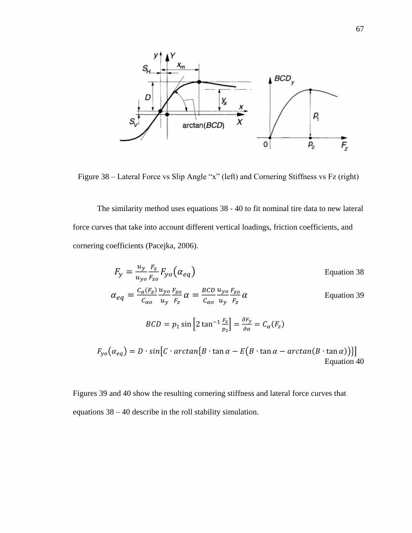
67

67

Figure 38 – Lateral Force vs Slip Angle “x” (left) and Cornering Stiffness vs Fz (right)

The similarity method uses equations 38 - 40 to fit nominal tire data to new lateral

force curves that take into account different vertical loadings, friction coefficients, and

cornering coefficients (Pacejka, 2006).

𝐹𝑦 =𝑢𝑦

𝑢𝑦𝑜

𝐹𝑧

𝐹𝑧𝑜𝐹𝑦𝑜(𝛼𝑒𝑞) Equation 38

𝛼𝑒𝑞 =𝐶𝛼(𝐹𝑧)

𝐶𝛼𝑜

𝑢𝑦𝑜

𝑢𝑦

𝐹𝑧𝑜

𝐹𝑧𝛼 =

𝐵𝐶𝐷

𝐶𝛼𝑜

𝑢𝑦𝑜

𝑢𝑦

𝐹𝑧𝑜

𝐹𝑧𝛼 Equation 39

𝐵𝐶𝐷 = 𝑝1 sin [2 tan−1 𝐹𝑧

𝑝2] =

𝜕𝐹𝑦

𝜕𝛼= 𝐶𝛼(𝐹𝑧)

𝐹𝑦𝑜(𝛼𝑒𝑞) = 𝐷 ∙ 𝑠𝑖𝑛[𝐶 ∙ 𝑎𝑟𝑐𝑡𝑎𝑛{𝐵 ∙ tan 𝛼 − 𝐸(𝐵 ∙ tan 𝛼 − 𝑎𝑟𝑐𝑡𝑎𝑛(𝐵 ∙ tan 𝛼))}]

Equation 40

Figures 39 and 40 show the resulting cornering stiffness and lateral force curves that

equations 38 – 40 describe in the roll stability simulation.

68

68

Figure 39 - Cornering Stiffness Curve Produced By Magic Formula for Simulation

Figure 40 - Lateral Force Curves Produced By Magic Formula

69

69

Once the 6 degree of freedom model had been built, the PUP’s geometry and

mass were then inputted into the model. The PUP’s roll stability was then tested by

running the vehicle through a series of steering and engine power inputs. Primarily the

vehicle would be given a sharp steering input, for example a 20 deg/s for one second

input, and then brake to simulate an avoidance maneuver. The vehicle was considered to

roll if the rear inner wheel of the turn lifted off the ground or had a vertical load of 0 N.

This simulation was run for a variety of CG locations, vehicle speeds, braking situations,

and steering inputs to determine the vehicle’s overall roll stability based on vertical wheel

loads.

The simulation was then used to find the vehicle’s lateral and longitudinal

acceleration in order to compare simulation results with the maximum lateral acceleration

possible based on equation 41. The terms ay and ax refer to the vehicle’s maximum lateral

acceleration before rollover and the associated longitudinal acceleration.

𝑎𝑦

𝑔=

𝑎𝑥

𝑔

𝑏

𝐿+

𝑏

ℎ

𝐿𝑓

𝐿 Equation 41

This equation was derived by summing the moments about the roll axis between the front

and rear tire and assuming that the vertical reaction force of one of the rear tires goes to

zero during the roll around the roll axis. Inertial forces were included in the derivation.

3.6 Summary

The assessment of the PUP required the use of both data acquisition and simulation

tools. Different systems can be applied to learn about different aspects of the vehicle.

GPS data can be used to keep a log of its daily use and help determine its overall impact

70

70

in sub-Saharan Africa. For the purposes of this paper, a DAQ system was developed to

measure and record strain in the frame of the PUP. LabVIEW was used along with NI

data acquisition hardware and a Wheatstone bridge to measure small voltage changes

from strain gauges. This data was then used to determine the stress in the frame at

specific locations. A finite element software (ANSYS) was then used to estimate the

actual forces acting on the frame while braking and driving over a series of bumps. Apart

from the data acquisition tools used in this assessment, a six degree of freedom model

was used to simulate a rollover event in MATLAB. This model was then compared to

steady state rollover equations in order to gain a better understanding about the PUP’s

roll stability.

71

71

CHAPTER 4. RESULTS AND DISCUSSION ON THE FRAME AND ROLL

STABILITY STUDY

4.1 Introduction

The PUP assessment primarily concentrated on two areas: frame analysis and roll

stability. A DAQ system was used to record strain gauge information as the utility

vehicle drove over a series of bumps. This information was then compared with a static

structural model in ANSYS in order to estimate the loads acting on the frame. The next

part of the assessment concentrated on the PUP’s roll stability. Steady state lateral

accelerations that caused rollover events were first calculated and then compared to a

dynamic simulation with six degrees of freedom. The simulated PUP was put through a

series of maneuvers to determine if wheel lift off occurred. The remainder of this chapter

concentrates on the findings from the frame analysis and roll stability study.

4.2 Frame Study Results

4.2.1 Strain Gauge Data

The results from the frame study gave greater definition as to what really happens

to the frame during normal vehicle operation. Data collected at 8 different strain gauge

locations provided information on the frame’s strength as the PUP drove over a series of

concrete stops at approximately 4 mph. It should be noted that a stress value of 0 MPa

corresponds to the stress when the PUP is static. Some of the

72

72

steel members were under stress due to the weight of the vehicle when the strain gauges

were calibrated, so that stress will read as 0 MPa during the experiments. Each concrete

stop was approximately 4.625 inches tall and 8.75 inches wide. In addition to the bump

test, data was also collected at certain strain gauge locations to determine the stress

induced into the frame due to braking. Video taken during the experiments helped

correlate the strain gauge data to physical events. Tire pressure was also taken. The

respective tire pressures for the front, rear right, and rear left tires were 20 psi, 18 psi, and

20 psi. The front tire was a 7.5L-15 tractor tire, and the rear tires were 95-16R-1 ribbed

tractor tires. Reducing the tire pressures would also reduce the stresses induced into the

frame as the tires would deflect more. Video showed that the rear tires deflected very

little.

Figure 41 plots the stresses induced into the frame member at the front strut 1

strain gauge position. Each concrete stop that the front tire hit produced large bending

stresses at the strain gauge location. Smaller driving disturbances like running over large

gravel stones or causing the vehicle to pitch forward by abruptly downshifting also

caused stress in this region. The ANSYS FEA simulation showed that this particular

position had a high stress gradient due to bending and caused correlating experimental

data with simulated data difficult. Figure 42 shows the captured data points while

sampling at a rate of 100 Hz while driving over a bump with the front and rear wheels.

73

73


Unloaded and Driving over Two Concrete Stops and Large Gravel


operating without a Load in the Bed While Driving over a Concrete Stop

Data collected in the left trailing arm area provided useful information toward

correlating the experimental data with the FEA model. The general trend during a rear

74

74

wheel contact event with the concrete block was that the trailing arm member was put

into tension before being compressed as the wheel rolled over the opposite side of the

concrete stop. Figure 44 shows the stress induced into the frame from the pillow block

attached to the trailing arm. When the trailing arm wheel hit the concrete stop, it pulled

on the pillow block and put the horizontal member attached to the pillow block in

tension.

Figure 43 - Strain Gauge Locations on the Rear Left Part of the Vehicle

75

75

Figure 44 – Strain Gauge Data for the Left Side Horizontal Member While the PUP

Drives Over a Concrete Stop with No Load (see figure 43 for location)

The data from the strain gauge mounted to the left side of the trailing arm showed

a similar pattern as the left side horizontal member only with higher stresses due to

bending. Figure 45 shows a sample of the data collected. As the vehicle drove over a

bump, the front wheel collision caused the trailing arm to compress as the rear wheels

pushed the front end over the bump. Then as the front tire rolled down the opposite side

of the bump, it pulled the rest of the vehicle and put the trailing arm member in tension.

Hitting the bump with the rear tire put the trailing arm in tension while rolling onto the

other side of the bump put it into compression. If the rear wheels did not hit the concrete

stop at the same time, the trailing arm would be put into torsion. This can be seen in

figure 45 showing the strain gauge data of the PUP driving over two concrete stops. As

the rear wheel landed on the other side of the concrete stop, the trailing arm would

occasionally bend causing high compressive stresses.

76

76

Figure 45 – Strain Gauge Data for the Left Trailing Arm Location When the PUP is

Unloaded and Driving over Two Closely Spaced Concrete Stops

The single rear wheel bump test gave further evidence for the bending stresses

induced into the frame. Figure 46 shows the stress induced into the left trailing arm

location when driving over a concrete stop with one wheel. The initial collision causes

the trailing arm to bend, then as the wheel rolls over the concrete block, the trailing arm

straightens and the tensile stress from the collision is induced. Finally, the largest bending

stress is induced when the wheel hits the ground on the other side of the concrete block.

This may be due to a combination of items including: an increase in rolling resistance

from increased vertical tire loads, higher inertial forces while falling than colliding with

the bump, and varying tire stiffness due to a larger tire contact area landing than hitting a

bump. The body of the PUP then rolls back and forth a few times as the mass of the

77

77

vehicle oscillates back and forth. These events can be seen in figure 46. Tables A1 and

A2 in the appendix summarize the data collected during the single rear wheel tire bump

test.


Unloaded and Driving over a Single Concrete Stop with only the Rear Left Wheel

The stress in the trailing arm increases when the mass suspended by the rear tires

increases. Applying a 1500 lb load in the bed of the PUP caused the tensile stress in the

left side of the trailing arm to increase from approximately 40 MPa to 90 MPa during a

single rear wheel hit. This can be seen in figure 47. The heavier bed load requires larger

inertial forces to lift the wheels over the bump causing larger stresses.

78

78



Single Concrete Stop with only the Rear Left Wheel

The front strut members experienced similar stress patterns as the rear trailing arm

where both the front and rear wheel impacts caused stress. This can be seen in figure 48

for data collected at the front strut 2 strain gauge position. Figure 48 shows a detailed

graph of the tire collision. It should be noted that the graph should be shifted up 18 MPa

to account for the stress induced on the member from the weight of the vehicle. All front

strut 2 graphs do not consider the stress due to the static weight of the vehicle. Initially,

the tire collision with the bump causes the strut member to be put into tension. Next, the

tire rolls down the other side of the bump causing a compressive stress. Finally, the tire

lands on the ground on the opposite side of the concrete bump causing a larger tensile

stress. The second, larger tensile stress may be due to the tire stiffness varying as the

contact area of the tire with the bump and ground varies. Video shows the tire deflecting

more and the strut spring less as it hits the concrete stop than when the tire lands on the

ground. When the tire hits the ground, the tire deflects very little which causes the

79

79

unsprung mass to move upward and compress the strut spring which introduces stress

into the frame members. Larger tire deflections during wheel collisions may decrease the

stress induced into the frame.

Figure 48 - Strain Gauge Values for the Front Strut 2 Location While the PUP is Loaded

with 1500 lb of Water and Driving Over a Single Concrete Stop

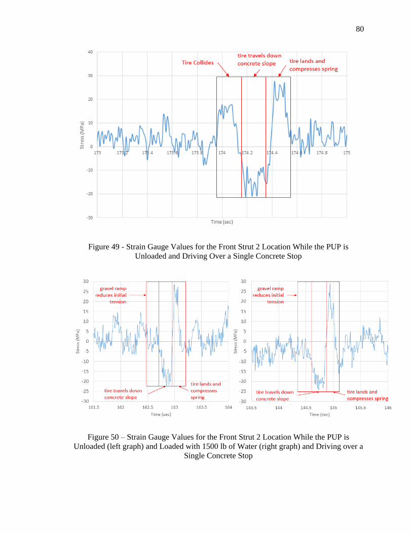
80

80

Figure 49 - Strain Gauge Values for the Front Strut 2 Location While the PUP is

Unloaded and Driving Over a Single Concrete Stop



Single Concrete Stop

81

81

This stress may be larger than the initial bending stress because the tire deflects

more during the initial collision than it does when it lands on the other side of the

concrete stop. The contact area on the tire is larger when it lands than when it hits the

concrete stop. This gives the tire a characteristic of having a higher spring stiffness

landing than hitting the concrete stop.

Table 6 – Average Experimental Stress Values for the Front Strut 2 Location While

Driving the PUP Unloaded Over a Single Concrete Stop (Excludes Static Weight Stress)

Event Value Units

Initial Tire Collision 16.0 MPa

Concrete Down Slope -20.9 MPa

Tire Hitting Ground 28.6 MPa

4.2.2 FEA Model Validation

ANSYS static structural models simulated the conditions that the PUP frame

endured during the experiments. The first static structural model represented hitting a

concrete stop with the rear wheels at the same time. Longitudinal forces acting at the

wheel hubs of the axle were increased until the Von Mises Stress at the strain gauge

location on the trailing arm equaled the average experimental values. Figures 51 and 52

represent the ANSYS model used for finding the necessary force loads.

82

82

Figure 51 – ANSYS Static Structural Simulation Showing Boundary Conditions for the

Trailing Arm Model While Hitting a Concrete Stop With Both Wheels


Trailing Arm Model While Hitting a Concrete Stop with Both Wheels

83

83

The model produced similar stress values as the experimental average with

longitudinal wheel loads of 9496 N. This correlates to a 4g acceleration for the rear mass

(484 kg) of the vehicle. Table 7 summarizes the results.


Trailing Arm Location for when the Two Rear Wheels Drive over a Concrete Stop

Value Units

Average Experimental Stress 20.89 MPa

Average Simulated Stress 20.4 MPa

Longitudinal Force Per Wheel 9496 N

Error -0.4 MPa

% Error 2.2 %

A similar model was used to predict the stresses induced into the frame from one

wheel hitting the concrete barrier. This model was based on video showing little spring

deflection while hitting the concrete stop when the PUP had no load in the bed. This led

to the idea that the trailing arm absorbed the majority of the impact. The FEA model

showed that assuming a 4g acceleration of the suspended mass of one wheel produced a

force that great enough to stress the trailing arm to values found in the experiment.

Figures 53 and 54 represent the model used. Table 8 summarizes the findings from

assuming a 4g acceleration.

84

84


Trailing Arm Model While Hitting a Concrete Stop With the Left Wheel When the PUP

is Unloaded


Trailing Arm Model While Hitting a Concrete Stop with the Left Rear Wheel

85

85


Trailing Arm Location for when the Left Rear Wheel Drives over a Concrete Stop When

the PUP is Unloaded

Value Units

Average Experimental Stress 41.1 MPa

Average Simulated Stress 49.4 MPa

Longitudinal Force Per Tire 9496 N

Lateral Force Per Tire 9496 N

Error 8.3 MPa

% Error 16.8 %

The front strut members were studied in a similar way as the rear trailing arm by

developing an ANSYS model with appropriate boundary conditions to mimic the actual

experiment. This model predicted a much smaller acceleration of the front mass of the

vehicle. This is most likely due to the suspension effects of the front strut. Much of the

force from the impact of the concrete stop is absorbed in the spring and front tire. Figures

55 and 56 represent the model used. The specific boundary conditions used were as

follows: the rear spring cups could not have displacements up or down (due to the

springs) and the pillow blocks that attached to the trailing arm could not have

displacements side to side or forward and backward (due to the trailing arm). A force was

applied to the front strut bracket that acted coaxially to the strut tower.

86

86


Front Strut Member Model While Hitting a Single Concrete Stop

87

87

Figure 56 - ANSYS Static Structural Simulation Showing Von Mises Stress for the Front

Strut Member Model While Hitting a Single Concrete

The front strut members experienced the largest amount of stress when the tire landed

back on the ground after driving over the concrete stop. The actual collision of the tire

with the concrete stop produced significantly less stress. The results between the two

collision events are summarized in tables 9 and 10.

88

88

Table 9 – Frame Study Summary with Static Stress Included for the Front Strut 2 Strain

Gauge Location for When an Unloaded PUP’s Front Tire First Collides with a Concrete

Stop (Stress Values Include the Stress From the Static Weight of the Vehicle)

Value Units

Mass suspended by front tire 292.1 kg

Acceleration of suspended mass 1.3 g’s

Inertial force acting on front strut frame bracket 3834 N

Average stress - tire collision 34.4 MPa

Average stress - simulated tire collision 37.7 MPa

Error -3.3 MPa

% Error 8.7 %

Table 10 - Frame Study Summary with Static Stress Included for the Front Strut 2 Strain

Gauge Location for When an Unloaded PUP’s Front Tire Rolls off the Concrete Stop and

Lands on The Ground (Stress Values Include the Stress From the Static Weight of the

Vehicle)

Value Units

Mass suspended by front tire 292.1 kg

Acceleration of suspended mass 1.6 g’s

Inertial force acting on front strut frame bracket 4718 N

Experimental average stress - tire hitting ground 47.0 MPa

Simulated average stress - tire hitting ground 46.8 MPa

Error 0.1 MPa

% Error 0.5 %

4.3 Roll Stability Results

4.3.1 Introduction to Roll Stability Study

The roll stability study of the PUP began by considering what maximum lateral

accelerations were needed to overturn the vehicle following equation 41. Next, the

89

89

dynamic roll stability simulation utilizing a 4th and 5th order Runge Kutta solver was used

to determine the vertical wheel reactions. The vehicle was considered to have rolled if

one of the rear wheels lifted off the ground or had a minimum wheel reaction of 0 N.

4.3.2 Maximum Lateral Acceleration Boundaries

The overall stability of the PUP can be determined by considering what lateral

accelerations are needed to cause the PUP to overturn. Equation 41 can be used to find

those boundaries. In the PUP’s case, braking while turning will lower the lateral

acceleration needed to cause the vehicle to overturn. The PUP’s geometry and measured

CG locations were used to determine the overall lateral stability.

90

90

Table 11 - Measured PUP Values and CG Locations (for geometry reference see figure

57)

Loading Condition Total

Mass

Distance From

Rear Axle To

CG (Lr)

Distance From

Front Wheel To

CG (Lf)

Height Of

CG (h)

Distance From

Centerline of

Vehicle to CG

- kg meters meters meters meters

0 driver, 0 passenger,

empty bed

615.5 1.06 1.62 Not

Available

-0.106


empty water tote

705.8 0.961 1.72 0.47 -0.098


empty bed

763.9 1.154 1.53 Not

Available

-0.104


empty water tote

781.1 1.0 1.66 Not

Available

-0.224


filled water tote

1145.3 0.598 2.08 Not

Available

-0.057


filled water tote

1386.2 0.501 2.18 Not

Available

-0.035


filled water tote

1463.3 0.557 2.12 Not

Available

-0.094

91

91

Figure 57 – 2015 PUP Center of Gravity (CG) Location and Geometry Notation

Table 12 - Measured Spring Rates

Spring Rate (N/m)

Front Spring 53721

Left Rear Spring 26015

Right Rear

Spring

23766

Avg. Rear Spring 24891

92

92

The measured values of the PUP showed that the CG location was about 1m away

from the rear axle (Lr = 1 m) in an unloaded case and 0.5m away from the rear axle (Lr =

0.5 m) in a loaded case. Additionally, the CG height was about 0.5 m high in an unloaded

case. These values along with the wheel base and track width of the PUP were used to

find that lateral acceleration limits of the vehicle. Figures 58 – 60 outline those lateral

acceleration boundaries before the vehicle rolls with respect to accelerating and

decelerating the vehicle at varying CG locations.

Figure 58 – Rollover Lateral Acceleration vs Braking and Accelerating at Varying CG

Heights When the CG is Located 1 Meter in Front of the Rear Axle (Lr = 1 m When PUP

is Unloaded)

93

93

Figure 59 - Rollover Lateral Acceleration vs Braking and Accelerating at Varying CG

Heights When the CG is Located 0.5 Meter in Front of the Rear Axle (Lr = 0.5 m When

PUP is Loaded)

Figure 60 – Rollover Lateral Acceleration vs Braking and Accelerating at Varying

Distances from the Rear Axle to the CG Location When the CG Height is 0.47 Meters

(h=0.47 m When PUP is Unloaded)

94

94

It is important to note that a vehicle is considered stable with respect to roll if

𝑎𝑦 > 𝜇 where ay is the lateral acceleration in g’s and μ is the coefficient of friction

between the tire and the ground (Huston et al., 1982). Assuming a maximum coefficient

of friction of 1, the PUP is considered stable with respect to roll as long as the rollover

lateral acceleration of the vehicle (which is based on the vehicle’s geometry, CG location,

and longitudinal acceleration) is above 1g. If this is true, the vehicle will slide outward in

a turn before it rolls. This is a conservative estimate as automotive tires have commonly

been found to produce maximum lateral accelerations of around 0.75 g’s (Van

Valkenburgh et al., 1982).

Figures 58 – 60 reveal many trends with respect to the PUP’s rollover stability.

To begin, the optimal placement of the CG for roll stability is between the rear wheels

centered over the rear axle as low to the ground as possible. The CG can never really be

all the way over the rear axle or on the ground because the front of the vehicle will have

some weight that pulls the CG forward, and the vehicle needs some ground clearance to

drive over rocks and bumps. The PUP’s current CG location in an unloaded case (no

driver, passengers, or payload) without braking or accelerating will most likely overturn

at lateral accelerations of approximately 0.88 g’s. Braking with 0.3 g’s of deceleration

lowers the overturn lateral acceleration to 0.8 g’s (assuming a CG location of 0.5 m off

the ground and 1 m in front of the rear axle). This shows that it is possible to roll the PUP

on surfaces and tires that produce friction coefficients greater than 0.8. So turning

aggressively on dry concrete with passenger tires while decelerating could cause the

vehicle to overturn. In a loaded case where the CG location is 0.5 m away from the rear

axle at a height of 0.6 m, the PUP has a rollover lateral acceleration of 0.95 g’s. Braking

95

95

at 0.3 g’s would bring that value to 0.87 g’s. Overall, the PUP has more roll stability in a

loaded case, and the least roll stability when a driver and passenger are sitting on the

front seats without a payload in the rear.

With the initial analysis of the PUP completed, the dynamic roll stability model

was used to determine what driving conditions would actually cause the PUP to roll by

reaching lateral accelerations greater than 0.8g’s. The initial simulation used the

parameters given in table A3 in the appendix. A rolling resistance coefficient of 0.08 was

used to represent a passenger tire rolling on a medium hard soil (Gawade et al., 2005).

The standard simulation considered a 20 degree steering angle which corresponds to a 7.7

m (25 feet) turning radius assuming there is no tire slip. The steering input was a ramped

response going from 0 to 20 degrees in one second for most simulations. Figures 61 and

62 give the outputted results of the six degree of freedom model.

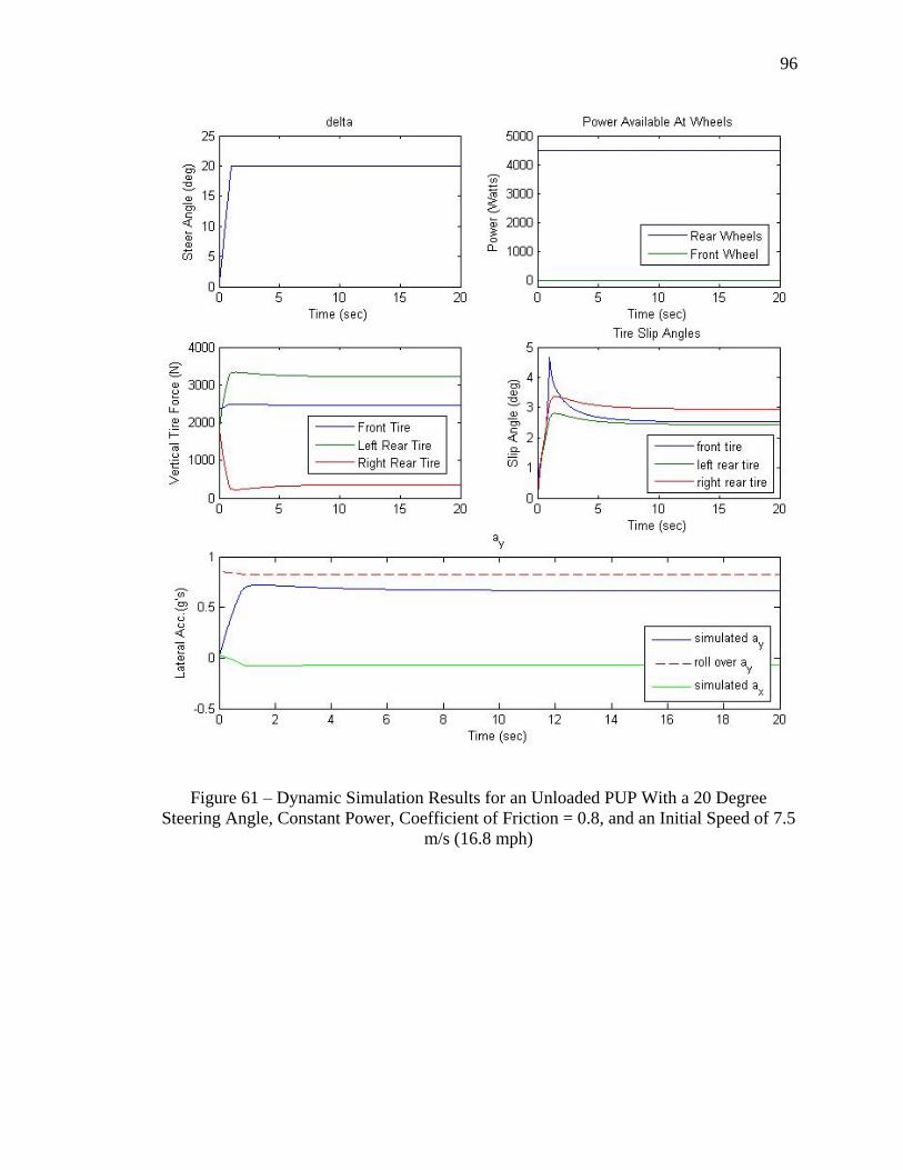
96

96

Figure 61 – Dynamic Simulation Results for an Unloaded PUP With a 20 Degree

Steering Angle, Constant Power, Coefficient of Friction = 0.8, and an Initial Speed of 7.5

m/s (16.8 mph)

97

97

Figure 62 – Principle Vehicle Motion Results from the Dynamic Simulation for an

Unloaded PUP with a 20 Degree Steering Angle, Constant Power, Coefficient of Friction

= 0.8, and an Initial Speed of 7.5 m/s (16.8 mph)

As can be seen in the graphs of figure 61 and 62, the PUP’s front tire is turned to

20 degrees in one second and held while a constant power is applied to the rear wheels to

drive the PUP forward at a near constant speed. The lateral inertial forces of the vehicle

cause the weight on the right tire (inner tire to the turn) to shift to the left tire (outside tire

98

98

to the turn). The right wheel comes close to losing contact with the road during the first

few seconds of the sharp turn as the vertical force on the tire dips down to a minimum

value, but then rises back up to a steady state value. Aggressive steering inputs and fast

speeds cause the PUP’s body to slightly overshoot its steady state roll angle. For the most

part, the simulated PUP has a relatively high roll stiffness. The graphs showing the

vertical wheel loads and the vehicle accelerations have a direct relation with each other.

The graph showing the simulated lateral acceleration along with the rollover acceleration

directly mimic the minimum wheel reaction graph. The dotted red line in the vehicle

acceleration graph represents equation 41 while the solid blue line represents the

simulated values from the 6 degree of freedom model. The minimum wheel reaction

approaches 0 N just as the simulated lateral acceleration approaches the rollover lateral

acceleration. This provides evidence that equation 41 can accurately predict the roll

stability of three wheeled vehicles.

During this simulated time, the simulated vehicle body rolls approximately 6

degrees while maintaining a pitch angle of nearly 0 degrees. Also, the height of the CG

remains at a near constant height. In reality, the PUP has additional roll stiffness from the

trailing arm, so it is expected that the vehicle’s body would roll around the roll axis of the

suspension even less than the simulated values. The relatively small roll angle, pitch

angle, and CG height of the simulated vehicle confirm the assumption of a near constant

CG location during vehicle operation.

Once the simulated values matched the general observations of driving the PUP,

the simulation was then used to see at what speed the PUP would rollover. When turning

the front wheel 20 degrees in a second while entering the turn at 30.4 mph, the simulated

99

99

PUP lost contact with the road briefly assuming a coefficient of friction of 0.8. This

would constitute a vehicle rollover. At higher speeds, the PUP barely loses contact with

the road for the first second because of the relatively sharp steering input, but remains in

contact with the road after that even at 45 mph. This is because the coefficient of friction

is nearly equal to the maximum lateral acceleration allowed before rollover. The PUP

tends to understeer and slide outward in the turn instead of rolling over.

Figure 63 – Dynamic Simulation Results for Roll Stability with a Coefficient of Friction

of 0.8 and Speed of 45mph

An unloaded PUP with a CG 1.06 meters away from the rear axle and a CG height of 0.5

meters will roll around 0.8 g’s of lateral acceleration. According to the simulation, the

PUP is at risk of rolling on surfaces with peak coefficients above 0.8. This can be seen in

figure 64 below where the peak coefficient of friction has been raised to 1. The PUP now

has wheel lift off around 7.6 m/s or 17 mph. In addition, the PUP body now rolls past 6

degrees during the initial turn.

100

100

Figure 64 - Dynamic Simulation Results for an Unloaded PUP Given a 20 Degree

Steering Angle in One Second, Constant Power, Coefficient of Friction = 1, and an Initial

Speed of 7.6 m/s (17 mph): P = 4.5 kW, upeak = 1

Braking and accelerating through turns can increase or decrease the PUP’s roll

stability to a certain degree. The roll stability simulation was run considering different

braking and accelerating events to gain a better understanding of their influence. The

simulation was run with a 20 degree steering input and a coefficient of friction of 0.8.

The first simulation set the baseline for the vehicle’s stability by running with constant

power. The second simulation powered the PUP with constant power for one second and

then braked all three wheels for three seconds once the maximum steer input had been

101

101

reached. The third simulation accelerated the vehicle by applying 8 kW of power at the

rear wheels after one second of constant power of 4.5 kW. Figure 65 shows the baseline

study where the vehicle enters a turn with constant power.

Figure 65 – Baseline Dynamic Simulation Results for an Unloaded PUP Assuming a

Coefficient of Friction = 0.8

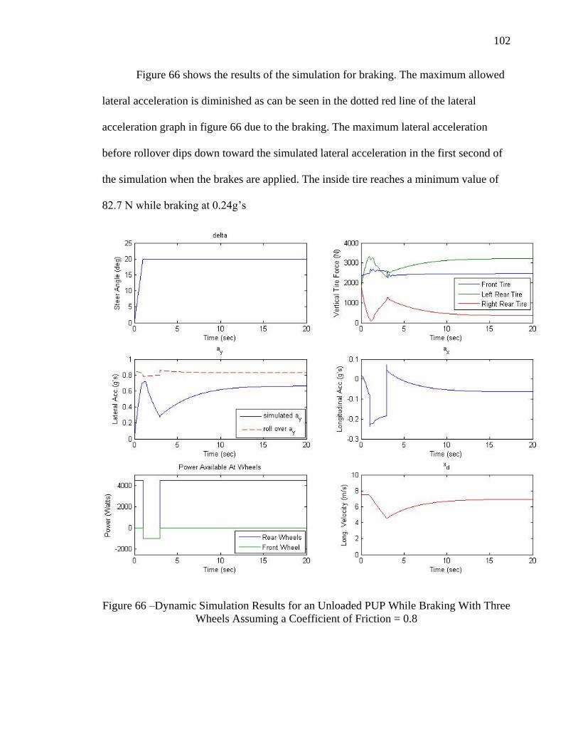
102

102

Figure 66 shows the results of the simulation for braking. The maximum allowed

lateral acceleration is diminished as can be seen in the dotted red line of the lateral

acceleration graph in figure 66 due to the braking. The maximum lateral acceleration

before rollover dips down toward the simulated lateral acceleration in the first second of

the simulation when the brakes are applied. The inside tire reaches a minimum value of

82.7 N while braking at 0.24g’s

Figure 66 –Dynamic Simulation Results for an Unloaded PUP While Braking With Three

Wheels Assuming a Coefficient of Friction = 0.8

103

103

Figure 67 summarizes the results from the acceleration simulation. Roll stability

increased as a measure of the minimum vertical wheel force. Table 13 summarizes the

overall roll stability of the PUP during the constant power, braking, and acceleration

events.

Figure 67 – Dynamic Simulation Results for an Unloaded PUP While Accelerating

Through a Turn Assuming a Coefficient of Friction = 0.8

104

104

Table 13 - Summary of Braking and Accelerating Simulations

Simulation Event Minimum Vertical Wheel Force (N)

Braking With Three Wheels 82.7

Constant Power 235.9

Accelerating 308.5

Figure 68 explores the PUP’s roll stability with a steering input going from 0° to

20° to -20° to 0°. The results mimicked that of the previous steering input only now the

weight shifted first to the left tire while turning right and then the right tire when turning

left. The minimum wheel forces were equal turning left and right.

Figure 68 - Dynamic Simulation Results for an Unloaded PUP Steering Right 20 Degrees

Then Left 20 Degrees and Finally Back to 0 Degrees Assuming a Coefficient of Friction

= 0.8

105

105

The previous simulations have provided the roll stability of the vehicle while

steering relatively aggressively toward the top speed of the PUP. The next simulation

study considers what the maximum steering input could be before the simulated PUP had

one of its wheels lift off the ground when a careful driver took a turn without pressing the

accelerator or brake. The steering input was slowly increased at constant engine power

with a peak coefficient of friction equal to 1. Figure 69 summarizes the simulated event.

Wheel liftoff occurred at a 25.4 degree steering input at 6.8 m/s (15.2 mph) at 0.82 lateral

g’s when a peak coefficient of friction of 1 is considered. When the simulation is re-run

with a peak coefficient of friction lower than 0.96, the PUP will begin to understeer and

never has a wheel liftoff event seen in figure 70.

106

106

Figure 69 - Dynamic Simulation Results for an Unloaded PUP When the Steering Input is

Slowly Increased Assuming a Coefficient of Friction = 1

Figure 70 – Roll Stability Represented By Vertical Tire Forces for an Unloaded PUP

When the Steering Input is Slowly Increased Assuming a Coefficient of Friction = 0.96

107

107

The simulation has shown that braking while turning can reduce the roll stability

of the vehicle, but it is unknown whether it is better to brake with the rear wheels verses

the front wheel. The simulation was next rerun with different braking scenarios

including: braking all three wheels, braking the front wheel, and braking the rear wheels.

In each case, a combined braking power of 2000 Watts was used between the front and

rear wheels. This simulation showed that braking with the front wheel brake only

produced the smallest wheel liftoff. This is partly because the braking power of one

wheel produced a slightly less deceleration. Figure 71 summarizes the event of braking

with all three wheels.

Figure 71 - Roll Stability When an Unloaded PUP Reaches a Steering Input of 20

Degrees and then Brakes with All Three Wheels While Pressing the Clutch

108

108

Table 14 - Roll Stability Study with Varying Braking Scenarios

Simulation Event Minimum Vertical

Wheel Force (N)

Braking

Deceleration (g’s)

Braking With Three Wheels 83 0.24

Braking With Rear Wheels 51 0.24

Braking With Front Wheel 117 0.23

Braking with the front wheel only is expected to produce the largest minimum

wheel reaction because it produces less of a braking acceleration. Combined braking is

advantageous because it produces less yaw due to the braking force on the front wheel

and produces the most braking power for quick stops. Braking with only the rear wheels

had the least stability.

So far this simulation has only considered the stability of the PUP in an unloaded

case. The simulation is now used to determine the roll stability of the vehicle at varying

CG locations. To begin, the distance from the rear axle to the CG location or Lr is

considered keeping the standard properties of the vehicle constant including a 20 degree

steering input and power input of 4.5 kW. Figure 72 summarizes the vehicle’s stability

with respect to the CG distance from the rear axle. The minimum vertical force on the

inside wheel to the turn decreases nearly linearly as the CG distance from the rear wheel

increases. The simulated lateral acceleration also increased as the CG location was

moved forward in the vehicle with the same steering input. Also, the vertical force wheel

reaction did not overshoot before reaching a steady state value. This shows that placing

the CG location directly over the rear axle has significant advantages.

109

109

Figure 72 – Roll Stability for an Unloaded PUP While Varying the Distance from the

Rear Axle to the CG (Lr) When the CG Height Equals 0.5 m (h = 0.5 m) (see figure 57

for PUP CG Location and Geometry Notation)

Next, the CG height was varied keeping the standard properties of the vehicle

constant including a 20 degree steering input, constant power input of 4.5 kW, Lr =

110

110

1.06m, peak coefficient of friction of 0.8, and an initial speed of 7.5 m/s 16.8 (mph).

Figure 73 shows the effects of varying the CG height. As can be seen in the graph

showing the minimum and steady state vertical force values of the inside tire (with

respect to the turn radius), the difference between the minimum force and steady state

force increases as the CG height increases. This shows that the vehicle body rolls more

aggressively with steering inputs with larger CG heights before settling to a steady state

roll angle. Decreasing the CG height to approximately 0.4 m would also make the vehicle

stable with respect to roll by increasing the rollover lateral acceleration to approximately

1g. In the unloaded state, the PUP will roll with the standard steering input with a CG

height of 0.56m.

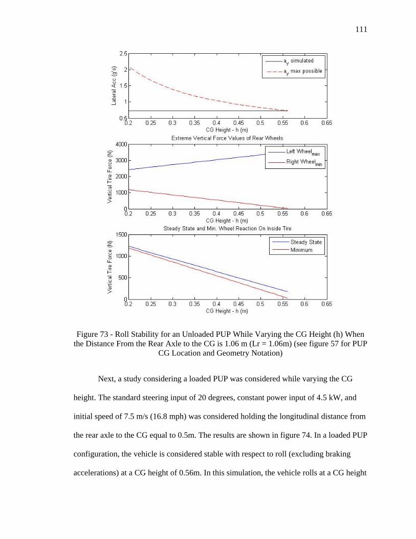
111

111

Figure 73 - Roll Stability for an Unloaded PUP While Varying the CG Height (h) When

the Distance From the Rear Axle to the CG is 1.06 m (Lr = 1.06m) (see figure 57 for PUP

CG Location and Geometry Notation)

Next, a study considering a loaded PUP was considered while varying the CG

height. The standard steering input of 20 degrees, constant power input of 4.5 kW, and

initial speed of 7.5 m/s (16.8 mph) was considered holding the longitudinal distance from

the rear axle to the CG equal to 0.5m. The results are shown in figure 74. In a loaded PUP

configuration, the vehicle is considered stable with respect to roll (excluding braking

accelerations) at a CG height of 0.56m. In this simulation, the vehicle rolls at a CG height

112

112

equal to 0.84 meters. This simulation provides evidence that the PUP could be made

completely stable with respect to roll (rollover lateral acceleration of 1g) if a load was set

between the rear wheels sitting low in the bed.

Figure 74 - Roll Stability for a Loaded PUP While Varying the CG Height (h) When the

Distance From the Rear Axle to the CG is 0.5 m (Lr = 0.5 m) (see figure 57 for PUP CG

Location and Geometry Notation)

113

113

CHAPTER 5. SUMMARY OF WORK

5.1 Strain Gauge and Video Study Findings

5.1.1 Frame Study Design Tools

The PUP frame study revealed several interesting findings that can be used in

future PUP designs. To begin, the video and strain gauge data collected for the frame

study showed that the some of the largest stresses recorded during the experiment

occurred in the trailing arm. Values close to 100 MPa were recorded. This makes sense

because the trailing arm does not have any mechanism to dampen the force longitudinally

when the rear wheel hits a bump. Also, the trailing arm can experience bending when a

single rear wheel hits a bump. The trailing arm experiences a tensile stress proportional to

the mass that is supported by the rear tires when it hits a bump. Tables 15 and 16

summarize the estimated vertical accelerations of the mass supported by the rear tires

when the rear wheels hit a bump.

Table 15 – Left Trailing Arm with No Load - Two Wheel Bump Summary

Value Units

Mass supported by rear tires 484 kg

vertical acceleration 4 g’s

Error -0.4 MPa

% Error 2.2 %

114

114

Table 16 – Left Trailing Arm with No Load - One Wheel Bump Summary

Value Units

Mass supported by rear tires 484 kg

Vertical acceleration 4 g’s

Error 8.3 MPa

% Error 16.8 %

The strain gauge experiments showed that the front strut members do not

experience significant changes in stress when the PUP is loaded verses unloaded. This

primarily is because the rear wheels take on the majority of the added weight.

Additionally, the collected video and strain gauge data showed that the front tire deforms

significantly and helps absorb the impact of running into the concrete stop. When the

front tire lands on the ground on the other side of the concrete stop, the stress induced

into the frame is higher which can be seen in the larger spring deflection and higher

induced stress in the strain gauge experiments. The data also showed that the combined

suspension effects of the front tire and coil spring on the front strut greatly reduce the

force from the concrete block in comparison to the rear trailing arm. This is reflected in

the estimated vertical acceleration of the mass that is supported by the front tire.

115

115


Values at the Front Strut Frame Member for When the Front Tire Initially Hits a

Concrete Stop

Value Units

Mass supported by front tire 292.1 kg

Vertical acceleration 1.3 g’s

Error -3.3 MPa

% Error 7.3 %


Values at the Front Strut Frame Member for When the Front Tire Lands on the Ground

on the Other Side of a Concrete Stop

Value Units

Mass supported by front tire 292.1 kg

Vertical acceleration 1.6 g’s

Error 0.1 MPa

% Error 0.5 %

The video data was also used in determining approximate decelerations of the

PUP while braking. Assuming constant deceleration, it was estimated that the PUP

experiences 0.4g’s while braking in an unloaded case and 0.2g’s in a loaded case.

116

116

Table 19 – Vehicle Vertical and Longitudinal Static Mass Acceleration Estimates

Value Unit

Vertical acceleration assumption with suspension damping 1.6 g’s

Vertical acceleration assumption with no suspension damping 4 g’s

Braking deceleration estimate of unloaded vehicle 0.41 g’s

Braking deceleration estimate of loaded vehicle 0.21 g’s

Table 19 can be used for developing future frame designs by implementing loads

into FEA models assuming a constant vertical acceleration. For example, the vertical

acceleration in table 19 for hitting a bump with no suspension can be used by first

assuming a bump hits a tire at a 45 degree angle and lifts the static mass supported by that

tire up at an acceleration of 4 g’s. The mass supported by that tire would then be

multiplied by the acceleration of 4 g’s to find the upward component of the force that lifts

the tire over the bump 𝐹𝑦 = 𝑚𝑠𝑡𝑎𝑡𝑖𝑐 × 4𝑔′𝑠. The longitudinal component of the force

acting at a 45 degree angle to the center of the tire would then equal the upward force

component since 𝐹𝑥 = 𝐹𝑦/ tan(45°) = 𝐹𝑦. The longitudinal accelerations can be used for

estimating the braking forces and also can be used for predicting the PUP’s roll stability.

5.1.2 Frame Study Durability Conclusions

The frame study on the PUP revealed that relatively low stresses are induced into

the frame while driving over approximately 5 inch tall bumps at 4 mph. When driven and

maintained appropriately, the PUP should not have any steel members yielding or failing

while operating on rough surfaces. The PUP frame is comprised of SAE 1020 steel that

117

117

has been hot rolled. This type of steel has a tensile strength of 380 MPa and a yield

strength of 210 MPa (Budynas, 2015). The left trailing arm strain gauge measured

stresses up to 100 MPa during bump test experiments, which is approximately half of the

yield stress. Although this stress is below the yield stress, this does not mean that the

trailing arm will not fail due to fatigue.

The experimental stresses were then compared to the endurance limit which is the

maximum stress that a steel member can endure for at least 1 million cycles without ever

failing due to fatigue. The endurance limit was calculated using methods from chapter 6

in Shigley’s Mechanical Engineering Design Ninth Edition (Budynas, 2015). The C-

channel on the trailing arm was considered to be bending and the angle iron members

were considered to be experiencing stresses axially since the frame is a truss shape. The

effects of corrosion were ignored, the properties of SAE 1020 steel were used, and a

reliability factor of 99.9% was used. As table 20 shows, frame stress should be kept

below 100 MPa in order to achieve infinite life. The data captured from the bump

experiments were largely below this value and suggest that the current PUP design

should not have fatigue values in the regions that the strain gauges were placed. Future

design teams should strive to keep stress values below 100 MPa in FEA simulations.

118

118

Table 20 – Endurance Limits For SAE 1020 Steel PUP Members

Endurance Limit Description Value Units

endurance limit for angle iron experiencing cyclical axial

stresses (size does not matter axially)

99 MPa

endurance limit for C-channel on trailing arm experiencing

cyclical bending stresses (30x30x3 mm angle iron)

98 MPa

endurance limit for C-channel on trailing arm experiencing

cyclical bending stresses (35x35x3.5 mm angle iron)

99 MPa

5.2 Roll Stability Findings

The maximum lateral acceleration that the PUP can experience before vehicle

rollover greatly depends on the track width, wheel base, CG height, and the longitudinal

distance from the rear axle to the CG. Additionally, braking can decrease the PUP’s

stability along with the road grade. The dynamic simulation closely matches the steady

state equation for roll stability since the PUP has such high roll stiffness. There is very

little overshoot for the minimum vertical tire force during an aggressive turn. As a result,

the steady state equation for roll stability can be used to predict vehicle overturn.

Equation 42 is the steady state roll stability equation with the effects of longitudinal

acceleration and road grade included. Braking corresponds to a negative acceleration, and

going downhill corresponds to a negative road grade angle. A friction coefficient between

0.8 and 1 can be equated to the lateral acceleration since it has been shown that the

maximum lateral acceleration possible before the vehicle slides is equal to the friction

119

119

coefficient for the given tire and driven surface. Figure 75 and table 21 describe the

variables used in equation 42. It should be noted that all accelerations are in g’s.

𝑎𝑦 = 𝑎𝑥𝑏

𝐿+

𝑏

ℎ

𝐿𝑓

𝐿cos 𝜃 +

𝑏

𝐿sin 𝜃 Equation 42

𝑤ℎ𝑒𝑟𝑒 𝑣𝑒ℎ𝑖𝑐𝑙𝑒 𝑖𝑠 𝑠𝑡𝑎𝑏𝑙𝑒 𝑤ℎ𝑒𝑛 𝜇 < 𝑎𝑦

Figure 75 – Description of Symbols for Steady State Rollover Equation

120

120

Table 21 – Description of Symbols for Equation 42

Symbol Description Units

μ friction coefficient -

ay lateral acceleration that causes wheel liftoff g’s

ax longitudinal acceleration due to accelerating (+) and braking (-) g’s

b Half of the vehicle track width m

L Vehicle wheel base m

h CG height off of ground m

Lf Distance from front wheel to CG m

θ road grade where uphill is positive and downhill is negative deg

The stability of the PUP can be greatly improved by setting general design goals and

loading the vehicle appropriately to ensure the CG is located in the appropriate position.

Equation 42 can be rearranged into equation 43 assuming a peak friction coefficient of 1

and a road grade of 0 degrees to calculate what CG height would be required to ensure

roll stability based on a braking deceleration and a longitudinal distance from the rear

axle. Using this CG height as a guideline allows the vehicle to slide before rolling. This

would be a conservative design guideline as it may not be possible to attain a 1g lateral

acceleration due to the PUP’s top speed of approximately 20 mph and in many cases the

peak coefficient of friction will be less than 1.

ℎ = 𝑏 (𝐿𝑓

𝐿) (1 −

𝑎𝑥

𝑔

𝑏

𝐿)

−1 Equation 43

121

121

Initial analysis implementing equation 41 showed that setting the CG height to 0.4

m (15.7 inches) for an unloaded PUP condition with the longitudinal distance from the

rear axle to the CG equal to 1 m provided the desired roll stability. The lateral

accelerations needed for the vehicle to rollover (without the effects of braking) would be

approximately 1 g. The measured PUP CG height without a driver was 0.47 m, so

lowering the CG height 7cm would meet the desired criteria.

The dynamic simulation that measured roll stability based off of minimum

vertical force of the inside tire of the turning radius confirmed many of the same trends

that were initially found. The simulated PUP was less stable while braking, but the

conditions had to be right to cause a rollover. Due to the PUP’s low top speed of 20 mph,

braking at the same time that the driver first turns the front wheel often slowed the

vehicle down enough initially during the braking event that relatively small lateral

accelerations were produced once the maximum steer angle had been reached. Braking at

the same moment that the maximum steer angle of 20 degrees had been reached produced

the least stability. This gives an indication on how the PUP should be operated in an

object avoidance maneuver.

Further investigation into braking compared braking with all three wheels, two

wheels, and one wheel. The simulation showed that braking with the front wheel showed

slight improvement for roll stability while braking with only rear wheels produced the

worst stability condition. Future PUP designs may emphasize the importance of having a

front brake for roll stability reasons.

Rollover conditions greatly depended on the coefficient of friction between the

road and tires of the PUP. It is reasonable to assume that the highest peak coefficients of

122

122

friction that occur between the tire and road will be between 0.8 and 1 as these values

correspond to a peak coefficient of friction for a tire rolling on a dry road at a tire’s rated

load (Gillespie, 1992). It is expected that the peak coefficient of friction would be more

towards 0.8 for the PUP since it will be driven primarily on compacted dirt roads. The

dynamic roll stability simulation produced the following results based on the criteria that

wheel liftoff resulted in rolling.

Table 22 - Simulation Results for Wheel Liftoff Events for an Unloaded PUP

coefficient

of friction

vehicle speed at

wheel liftoff (mph)

steering angle

(deg)

0.8 30.4 20

1 16.7 20

1 15.2 25.4

The last row in table 22 corresponds to a wheel liftoff event when the steering angle is

slowly increased by 1 degree per second.

Simulations have shown that the ideal placement of the CG for the PUP is

between the rear wheels and as low as possible. Future design recommendations for the

PUP would be as follows in order to prevent rollovers from improper loading.

lower the CG 7 cm in an unloaded PUP case

o Alternative: move the CG toward rear axle approximately 20 cm in

unloaded case

123

123

o Alternative: both lower the CG and move toward rear axle for unloaded

case using 7cm and 20cm as guidelines

prevent bed loadings that raise the CG height above 0.6 m for a loaded case

124

WORKS CITED

124

124

WORKS CITED

Adelekan, B. A. (2012). Heightened impacts of agricultural engineering in raising the

productivity of Nigerian agriculture. Paper presented at the Creating a

competitive edge through agricultural mechanization and post-harvest technology

in developing countries. International Conference of Agricultural Engineering-

CIGR-AgEng 2012: Agriculture and Engineering for a Healthier Life, Valencia,

Spain, 8-12 July 2012.

Alibaba. (2016). Multi-function Two Wheel Mini Walking Tractor. Retrieved from

http://www.alibaba.com/product-detail/Multi-function-two-wheel-mini-

walking_60373092082.html

Alibaba Manufacturer Directory - Suppliers, Manufacturers, Exporters & Importers.

(2016). Retrieved from

http://gzdengfeng.en.alibaba.com/productshowimg/817587282-

210110587/KAVAKI_MOTOR_150CC_motorbike.html

Bank, T. W. (2016). Jobs Data for Sub Saharan Africa: World Bank. Retrieved from

http://datatopics.worldbank.org/jobs/region/sub-saharan-africa

Benin, S. (2015). Impact of Ghana's agricultural mechanization services center program.

Agricultural Economics, 46(S1), 103-117. doi:10.1111/agec.12201

Binswanger-Mkhize, H. P. (1984). Agricultural mechanization : a comparative historical

perspective. Washington, D.C.: Washington, D.C. : World Bank.

Bishop-Sambrook, C. (2005). Contribution of farm power to smallholder livelihoods in

sub-Saharan Africa (1814-1137). Retrieved from Rome:

http://www.fao.org/docrep/009/a0229e/a0229e00.HTM

Briney, A. (2015). All You Wanted to Know about the Green Revolution. Retrieved from

http://geography.about.com/od/globalproblemsandissues/a/greenrevolution.htm

Budynas, R. G. (2015). Shigley's mechanical engineering design (Tenth edition / Richard

G. Budynas, professor emeritus, Kate Gleason College of Engineering, Rochester

Institute of Technology, J. Keith Nisbett, associate professor of mechanical

engineering, Missouri University of Science and Technology.. ed.): New York,

NY : McGraw-Hill.

Motor Vehicle Safety Regulations (C.R.C., c. 1038) - Transport Canada,

(modified:2016-04-07).

http://www.alibaba.com/product-detail/Multi-function-two-wheel-mini-walking_60373092082.html

http://www.alibaba.com/product-detail/Multi-function-two-wheel-mini-walking_60373092082.html

http://gzdengfeng.en.alibaba.com/productshowimg/817587282-210110587/KAVAKI_MOTOR_150CC_motorbike.html

http://gzdengfeng.en.alibaba.com/productshowimg/817587282-210110587/KAVAKI_MOTOR_150CC_motorbike.html

http://datatopics.worldbank.org/jobs/region/sub-saharan-africa

http://www.fao.org/docrep/009/a0229e/a0229e00.HTM

http://geography.about.com/od/globalproblemsandissues/a/greenrevolution.htm

125

125

Case, J., Chilver, L., & Ross, C. T. F. (1999). 2 - Pin-jointed frames or trusses Strength of

Materials and Structures (Fourth Edition) (pp. 55-66). London: Butterworth-

Heinemann.

ChartsBin. (2011). Worldwide Total Motor Vehicles (per 1,000 people). Retrieved from:

http://chartsbin.com/view/1114

Classics, S. J. (2016). Jaguar´s Winning Sports Car the C-type. Jaguar Heritage

Magazine, (5). Retrieved from Suffolk Jaguar Classics website:

http://www.suffolksportscars.com/suffolk-c-type/jaguar-history/history

Connor, J. J., & Faraji, S. (2012). Fundamentals of structural engineering: Springer

Science & Business Media.

Corona, E. (2015). Data Acquisition System. Retrieved from

de Oliveira, F. C. G., & Borges, J. A. F. (2008). Design and Optimization of a Space

frame Chassis. http://dx.doi.org/10.4271/2008-36-0253

Dixon, J., Tanyeri-Abur, A., & Horst, W. (2004). Framework For Analysing Impacts of

Globalization On Smallholders Smallholders, globalization and policy analysis.

Rome: Food and Agriculture Organization of the United Nations.

FAO, IFAD, & WFP. (2015). The State of Food Insecurity in the World 2015. Meeting

the 2015 international hunger targets: taking stock of uneven progress.

FAOSTAT. (2016). Food Security, Suite of Food Security Indicators.

http://faostat3.fao.org/download/D/FS/E

Gawade, T., Mukherjee, S., & Mohan, D. (2005). Six-degree-of-freedom three-wheeled-

vehicle model validation. Proceedings of the Institution of Mechanical Engineers,

Part D: Journal of Automobile Engineering, 219(4), 487-498.

Gillespie, T. D. (1992). Fundamentals of vehicle dynamics. Warrendale, PA: Warrendale,

PA : Society of Automotive Engineers.

Godfray, H. C. J., Beddington, J. R., Crute, I. R., Haddad, L., Lawrence, D., Muir, J.

F., . . . Toulmin, C. (2010). Food Security: The Challenge of Feeding 9 Billion

People. Science, 327(5967), 812-818. doi:10.1126/science.1185383

Hine, J. (2014). Good Policies and Practices on Rural Transport in Africa: Planning

Infrastructure and Services. Good Policies and Practices on Rural Transport in

Africa: Planning Infrastructure and Services.

Hirai, M., Ueno, T., Iwaki, Y., & Oohama, S. (2013). Application of FEM Analysis Using

Loads Predicted from Strain Measurements in Motorcycle Frame Development.

Retrieved from Japan:

Holloway, D. C., Drach, T. J., & Mohanty, B. (1991). An Experimental Investigation of

Passenger Car Tire Properties at High Slip and Camber Angles.

http://dx.doi.org/10.4271/910233

http://chartsbin.com/view/1114

http://www.suffolksportscars.com/suffolk-c-type/jaguar-history/history

http://dx.doi.org/10.4271/2008-36-0253

http://faostat3.fao.org/download/D/FS/E

http://dx.doi.org/10.4271/910233

126

126

Horn, A. (2016). Corporate Nigeria - Agriculture Overview - Agriculture Overview.

Retrieved from http://www.corporate-

nigeria.com/index/agriculture/agriculture_overview.html

Houmy, K., & FAO. (2013). Agricultural mechanization in sub-Saharan Africa :

guidelines for preparing a strategy. Rome: Rome : Plant Production and

Protection Division, Food and Agriculture Organization of the United Nations.

Houmy, K., & Food and Agriculture Organization of the United Nations. Plant

Production and Protection, D. (2013). Agricultural mechanization in sub-Saharan

Africa : guidelines for preparing a strategy. Rome: Rome : Plant Production and

Protection Division, Food and Agriculture Organization of the United Nations.

Huston, J. C., Graves, B. J., & Johnson, D. B. (1982). Three wheeled vehicle dynamics.

Retrieved from http://papers.sae.org/820139/

Instruments, N. (2016). Strain Gauge Configuration Types - National Instruments.

Retrieved from http://www.ni.com/white-paper/4172/en/

Jain, A. (2014). Computational Analysis and Optimization of Torsional Stiffness of a

Formula-SAE Chassis. http://dx.doi.org/10.4271/2014-01-0355

Johnson, D. H. (1986). Finite Element Design Optimization of the WABCO 170 Ton

Haulpak Truck Frame. http://dx.doi.org/10.4271/860748

Kienzle, J., Ashburner, J. E., & Sims, B. (2013). Mechanization for rural development: A

review of patterns and progress from around the world. Retrieved from

Lovson. (2016). Autorickshaw â�“ Delivery Van, Pickup Van, Passenger Van, Indian 3

Wheelers, Rickshaw, Tuk Tuk, Tuc Tuc. Retrieved from http://www.auto-

rickshaw.com/pickup-standard.html

Lumkes, J. H. (2012). Design of a sustainable, locally manufacturable, agricultural utility

vehicle for developing countries. … 2012: agriculture and engineering for a ….

Pacejka, H. B. (2006). Chapter 4 - Semi-empirical tyre models Tyre and Vehicle

Dynamics (Second Edition) (pp. 156-215). Oxford: Butterworth-Heinemann.

Pasquini, E. (2016). '�˜Can we feed the world?'�™: A conversation with Sir Gordon

Conway | Devex. Retrieved from https://www.devex.com/news/can-we-feed-the-

world-a-conversation-with-sir-gordon-conway-80598

Raman, A., Rao, J. S., & Kale, S. R. (1995). Overturning Stability of Three Wheeled

Motorized Vehicles. Vehicle System Dynamics, 24(2), 123-144.

doi:10.1080/00423119508969084

Riley, W. B., & George, A. R. (2002). Design, Analysis and Testing of a Formula SAE

Car Chassis. http://dx.doi.org/10.4271/2002-01-3300

Riverson, J., & Carapetis, S. (1991). Intermediate means of transport in Sub-Saharan

Africa. World Bank technical paper, 161.

Rosegrant, M. W., & Cline, S. A. (2003). Global Food Security: Challenges and Policies.

Science Magazine, 302(5652), 1917-1919. doi:10.1126/science.1092958

http://www.corporate-nigeria.com/index/agriculture/agriculture_overview.html

http://www.corporate-nigeria.com/index/agriculture/agriculture_overview.html

http://papers.sae.org/820139/

http://www.ni.com/white-paper/4172/en/

http://dx.doi.org/10.4271/2014-01-0355

http://dx.doi.org/10.4271/860748

http://www.auto-rickshaw.com/pickup-standard.html

http://www.auto-rickshaw.com/pickup-standard.html

https://www.devex.com/news/can-we-feed-the-world-a-conversation-with-sir-gordon-conway-80598

https://www.devex.com/news/can-we-feed-the-world-a-conversation-with-sir-gordon-conway-80598

http://dx.doi.org/10.4271/2002-01-3300

127

127

Seck, P. A. (2011). Feeding the world in 2050. Rice Today, 10(4), 12-13.

Takeshima, H., Min-Pratt, A., & Xinshen, D. (2013). MECHANIZATION AND

AGRICULTURAL TECHNOLOGY EVOLUTION, AGRICULTURAL

INTENSIFICATION IN SUB-SAHARAN AFRICA: TYPOLOGY OF

AGRICULTURAL MECHANIZATION IN NIGERIA. American Journal of

Agricultural Economics, 95(5), 1230-1236. doi:10.1093/ajae/aat045

Tuk-tuking the world by storm. (2014). Retrieved from

http://www.economist.com/news/business/21596993-motorised-rickshaw-despite-

official-disapproval-becoming-ubiquitous-tuk-tuking

United States. Flight Standards, S., Aviation, S., amp, & Academics, I. (2012). Aviation

maintenance technician handbook. Airframe. Newcastle, Wash.: Newcastle,

Wash. : Aviation Supplies & Academics.

Van Valkenburgh, P. G., Klein, R. H., & Kanianthra, J. (1982). Three-Wheel Passenger

Vehicle Stability and Handling. http://dx.doi.org/10.4271/820140

Wen, J. H. (2008). Virtual Prototyping in Redesign and Durability Test Assessment. SAE

Int. J. Mater. Manf., 1(1), 441-449. doi:10.4271/2008-01-0862

Zorya, S., Morgan, N., Rios, D. L., Hodges, R., & Bennett, B. (2011). Missing food: the

case of postharvest grain losses in sub-Saharan Africa. Missing food: the case of

postharvest grain losses in sub-Saharan Africa.

http://www.economist.com/news/business/21596993-motorised-rickshaw-despite-official-disapproval-becoming-ubiquitous-tuk-tuking

http://www.economist.com/news/business/21596993-motorised-rickshaw-despite-official-disapproval-becoming-ubiquitous-tuk-tuking

http://dx.doi.org/10.4271/820140

128

APPENDIX

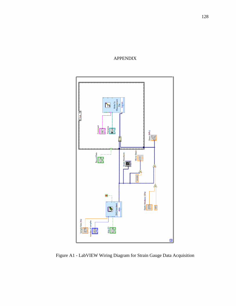
128

APPENDIX

Figure A1 - LabVIEW Wiring Diagram for Strain Gauge Data Acquisition

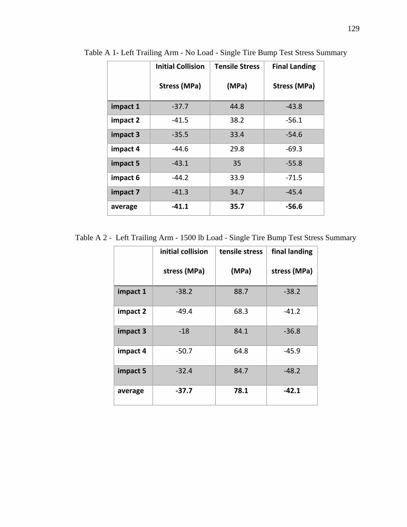
129

Table A 1- Left Trailing Arm - No Load - Single Tire Bump Test Stress Summary

Initial Collision

Stress (MPa)

Tensile Stress

(MPa)

Final Landing

Stress (MPa)

impact 1 -37.7 44.8 -43.8

impact 2 -41.5 38.2 -56.1

impact 3 -35.5 33.4 -54.6

impact 4 -44.6 29.8 -69.3

impact 5 -43.1 35 -55.8

impact 6 -44.2 33.9 -71.5

impact 7 -41.3 34.7 -45.4

average -41.1 35.7 -56.6

Table A 2 - Left Trailing Arm - 1500 lb Load - Single Tire Bump Test Stress Summary

initial collision

stress (MPa)

tensile stress

(MPa)

final landing

stress (MPa)

impact 1 -38.2 88.7 -38.2

impact 2 -49.4 68.3 -41.2

impact 3 -18 84.1 -36.8

impact 4 -50.7 64.8 -45.9

impact 5 -32.4 84.7 -48.2

average -37.7 78.1 -42.1

130

130

Table A 3 – Roll Stability Dynamic Simulation Parameters

Value Unit Description

L 2.675 m wheel base

Lr 1.06 m distance from rear axle to CG

ho 0.5 m CG height

tw 1.4 m track width

b 0.7 m halftrack width

m 615.5 kg total mass (no driver, passenger, or load)

Ix 76.78 kg-m^2 mass moment of inertia about x-axis

Iy 400.4 kg-m^2 mass moment of inertia about y-axis

Iz 421.93 kg-m^2 mass moment of inertia about z-axis

C_1 28648 N/rad cornering stiffness of front tire

C_2 34377 N/rad cornering stiffness of rear tire

u_p 0.8 N/N peak coefficient of friction while rolling

f 0.08 N/N rolling resistance coefficient

k1 53721 N/m spring rate of front spring

k2 24891 N/m spring rate of rear spring

k1_t 200000 N/m spring rate of front tire

k2_t 200000 N/m spring rate of rear tire

c 1000 N-s/m damping coefficient

131

131

Roll Stability Simulation MATLAB Code

Main Script File: “Roll_Stability_Transient5.m” %Roll Stability - Transient Roll Simulation %By: Jeremy Robison %%%%%%%%%%%%%%%%%%%%%%%%%%%%%%%%%%%%%%%%%%%%%%%%%%%%%%%%%%%%%%%%%%%%%%%

%%%%%%%%%%%%%%%%%%%%%%%%%%%% %Description: %This simulation determines the transient roll stability of a three

wheeled vehicle with a single tire in the front. %This simulation takes the inputed vehicle geometry, tire %characteristics, suspension characteristics, engine power, and tire

steering angle to %determine the forces acting on the three wheels of the vehicle during

a %turn. Various CG locations, steering inputs, braking power, and

acceleration power inputs are used. %%%%%%%%%%%%%%%%%%%%%%%%%%%%%%%%%%%%%%%%%%%%%%%%%%%%%%%%%%%%%%%%%%%%%%%

%%%%%%%%%%%%%%%%%%%%%%%%%%% close clear clc

n = 1; %initialize counter %TIME INPUTS t_span = [0 20];

%VEHICLE GEOMETRY AND MASS L = 2.675; %(m) wheel base (2.675) %for Lr = 0.1:0.05:1.26; %(m) distance from rear axle to CG Lr = 1.06; %(m) distance from rear axle to CG (1.06) %for ho = 0.2:0.01:0.56 ho = 0.5; %(m) static height of CG (0.5) tw = 1.4; %(m) track width of vehicle (1.4)

m = 615.5; %(kg) mass of vehicle (615.5) g = 9.81; %(m/s^2) acceleration of gravity Ix = 76.78; %(kg-m^2) Principle moments of inertia of vehicle body

(76.78) Iy = 400.4; %(kg-m^2) Principle moments of inertia of vehicle body

(400.4) Iz = 421.93; %(kg-m^2) Principle moments of inertia of vehicle body

(421.93)

Lf = L-Lr; %(m) distance from front strut to CG b = tw/2; %(m) half track width of vehicle

%TIRE CHARACTERISTICS C_1 = 28648; %(N/rad) cornering stiffness %450 N/deg for 14inch

wheel(28648) C_2 = 34377; %(N/rad) cornering stiffness %600 N/deg for 15inch wheel

(34377) C_3 = C_2; %(N/rad) cornering stiffness

132

132

u_p = 0.8; %(N/N)peak coefficient of friction ranges from 0.05 to 1

f = 0.08; %(N/N) rolling resistance coefficient (0.08)

%SUSPENSION CHARACTERISTICS k1 = 53721; %(N/m) spring rate of front tire (53721) %for k2 = 5000:1000:25000; %(N/m) spring rate of left tire k2 = 24891; %(N/m) spring rate of left tire (24891) k3 = k2; %(N/m) spring rate of right tire

k1_t = 200000; %(N/m) stiffness of front tire (160000 N/m from p.163 in

Gillespie) k2_t = 200000; %(N/m) stiffness of rear tire

k1_eq = k1_t*k1/(k1+k1_t); %equivalent spring force due to spring and

tire k2_eq = k2_t*k2/(k2+k2_t); %equivalent spring force due to spring and

tire

c1 = 1000; %(N-s/m) damping coefficient of front tire (980 N-s/m p.163

in Gillespie) c2 = c1; %(N-s/m) damping coefficient of left tire c3 = c1; %(N-s/m) damping coefficient of right tire c = c1; %all damping coefficients are equal

%ROAD INPUT theta_deg = 0; %(deg) road grade theta = theta_deg*pi/180; %(rad) road grade

%Initialize x = 0; x_d =7.5; %forward speed (max of 8.9)7.5 y = 0; y_d = 0; %lateral speed z = 0; z_d = 0; %downward speed psi = 0; %yaw angle psi_d = 0; %yaw rate phi = 0; %roll angle phi_d = 0; %roll rate chi = 0; %pitch angle chi_d = 0; %pitch rate

u_0 = [x;x_d;y;y_d;z;z_d;psi;psi_d;phi;phi_d;chi;chi_d]; %store initial

values

%% options = odeset('AbsTol',1e-10,'RelTol',1e-10); [t,u] = ode45(@(t,u)

roll_matrix5(t,u,m,f,C_1,C_2,b,Lr,Lf,L,k1_eq,k2_eq,c,g,Ix,Iy,Iz,ho,u_p)

,t_span,u_0); %Explicit Runge-Kutta (4th and 5th order)

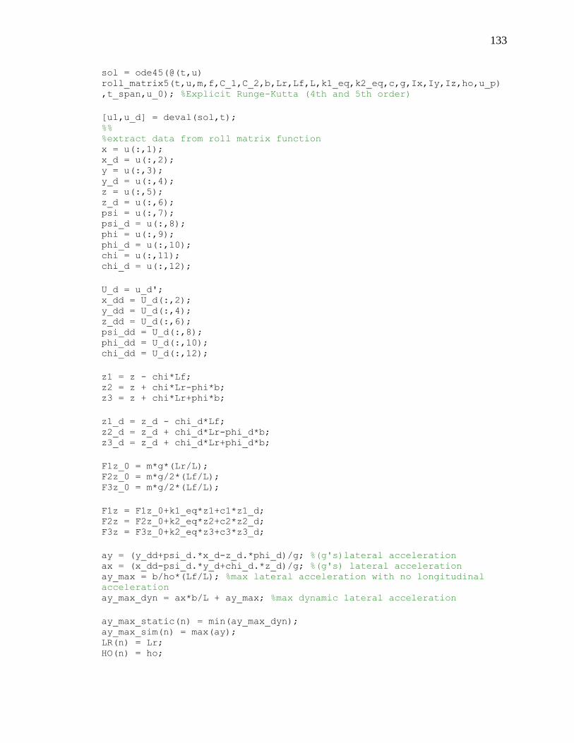
133

133

sol = ode45(@(t,u)


,t_span,u_0); %Explicit Runge-Kutta (4th and 5th order)

[u1,u_d] = deval(sol,t); %% %extract data from roll matrix function x = u(:,1); x_d = u(:,2); y = u(:,3); y_d = u(:,4); z = u(:,5); z_d = u(:,6); psi = u(:,7); psi_d = u(:,8); phi = u(:,9); phi_d = u(:,10); chi = u(:,11); chi_d = u(:,12);

U_d = u_d'; x_dd = U_d(:,2); y_dd = U_d(:,4); z_dd = U_d(:,6); psi_dd = U_d(:,8); phi_dd = U_d(:,10); chi_dd = U_d(:,12);

z1 = z - chi*Lf; z2 = z + chi*Lr-phi*b; z3 = z + chi*Lr+phi*b;

z1_d = z_d - chi_d*Lf; z2_d = z_d + chi_d*Lr-phi_d*b; z3_d = z_d + chi_d*Lr+phi_d*b;

F1z_0 = m*g*(Lr/L); F2z_0 = m*g/2*(Lf/L); F3z_0 = m*g/2*(Lf/L);

F1z = F1z_0+k1_eq*z1+c1*z1_d; F2z = F2z_0+k2_eq*z2+c2*z2_d; F3z = F3z_0+k2_eq*z3+c3*z3_d;

ay = (y_dd+psi_d.*x_d-z_d.*phi_d)/g; %(g's)lateral acceleration ax = (x_dd-psi_d.*y_d+chi_d.*z_d)/g; %(g's) lateral acceleration ay_max = b/ho*(Lf/L); %max lateral acceleration with no longitudinal

acceleration ay_max_dyn = ax*b/L + ay_max; %max dynamic lateral acceleration

ay_max_static(n) = min(ay_max_dyn); ay_max_sim(n) = max(ay); LR(n) = Lr; HO(n) = ho;

134

134

F3z_min(n) = min(F3z); %minimum wheel value of inside wheel F3z_ss(n) = F3z(numel(t)); %steady state value of inside wheel F2z_max(n) = max(F2z); %maximum wheel value of outside wheel F2z_ss(n) = F2z(numel(t)); %steady state value of outside wheel k(n) = k2_eq;

n=n+1; %end

%use data from roll matrix to find more data for results num = numel(t); for q = 1:num; time = t(q);

[delta] = steer_fun3(time); [P,P_brake] = power_fun1(time); steer_angle(q) = delta; power(q) = P; p_brake(q) = P_brake;

a1(q) = -(atan((y_d(q)+Lf*psi_d(q))/x_d(q)) - steer_angle(q)); a2(q) = -atan((y_d(q)-Lr*psi_d(q))/(x_d(q)+b*psi_d(q))); a3(q) = -atan((y_d(q)-Lr*psi_d(q))/(x_d(q)-b*psi_d(q)));

%Pacejka Magic Formula [F1_tire] = magic_formula(a1(q),F1z(q),u_p,C_1); F1y(q) = F1_tire*cos(delta) + (p_brake(q)/x_d(q)-f*F1z(q))*sin(delta);

%Left Rear Tire [F2_tire] = magic_formula(a2(q),F2z(q),u_p,C_2); F2y(q) = F2_tire;

%Right Rear Tire [F3_tire] = magic_formula(a3(q),F3z(q),u_p,C_2); F3y(q) = F3_tire;

end P_brake = P_brake'; steer_angle = steer_angle'; power = power';

%% phi = phi*180/pi; chi = chi*180/pi; steer_angle = steer_angle*180/pi; a1 = a1*180/pi; a2 = a2*180/pi; a3 = a3*180/pi; %Results % figure(1) % subplot(3,2,1) % plot(t,x_d,'-r')

135

135

% title('x_d') % ylabel('Long. Velocity (m/s)') % xlabel('Time (sec)') % axis([0 t(q) 0 10]) % % subplot(3,2,2) % plot(t,y_d,'-r') % title('y_d') % ylabel('Lat. Velocity (m/s)') % % subplot(3,2,3) % plot(t,z,'-r') % title('z') % ylabel('Vertical Position of CG (m)') % axis([0 t(q) -0.01 0.01]) % % subplot(3,2,4) % plot(t,phi,'-r') % title('phi') % ylabel('Roll Angle(deg)') % % subplot(3,2,5) % plot(t,psi_d,'-r') % title('psi_d') % ylabel('Yaw (rad/s)') % % subplot(3,2,6) % plot(t,chi,'-r') % title('chi') % ylabel('Pitch Angle (deg)')

% figure(2) % plot(t,a1,t,a2,t,a3) % ylabel('Slip Angle (deg)') % xlabel('Time (sec)') % legend('alpha_1','alpha_2','alpha_3') %hold on

% figure(3) % subplot(3,1,1) % plot(LR,ay_max_sim,'-k',LR,ay_max_static,'--r') % xlabel('CG Distance From Rear Axle - Lr (m)') % ylabel('Lateral Acc (g''s)') % legend('a_y simulated','a_y max possible') % % subplot(3,1,2) % plot(LR,F2z_max,'-b',LR,F3z_min,'-r') % legend('Left Wheel_m_a_x','Right Wheel_m_i_n') % ylabel('Vertical Tire Force (N)') % xlabel('CG Distance From Rear Axle - Lr (m)') % title('Extreme Vertical Force Values of Rear Wheels') % axis([0 1.3 0 4500]) % % subplot(3,1,3) % plot(LR,F3z_ss,'-b',LR,F3z_min,'-r')

136

136

% legend('Steady State','Minimum') % ylabel('Vertical Tire Force (N)') % xlabel('CG Distance From Rear Axle - Lr (m)') % title('Steady State and Min. Vertical Tire Forces On Inside Tire') % axis([0 1.3 0 2000])

% figure(4) % subplot(3,1,1) % plot(HO,ay_max_sim,'-k',HO,ay_max_static,'--r') % xlabel('CG Height - h (m)') % ylabel('Lateral Acc (g''s)') % legend('a_y simulated','a_y max possible') % % subplot(3,1,2) % plot(HO,F2z_max,'-b',HO,F3z_min,'-r') % legend('Left Wheel_m_a_x','Right Wheel_m_i_n') % ylabel('Vertical Tire Force (N)') % xlabel('CG Height - h (m)') % title('Extreme Vertical Force Values of Rear Wheels') % %axis([0 1.3 0 4500]) % % subplot(3,1,3) % plot(HO,F3z_ss,'-b',HO,F3z_min,'-r') % legend('Steady State','Minimum') % ylabel('Vertical Tire Force (N)') % xlabel('CG Height - h (m)') % title('Steady State and Min. Wheel Reaction On Inside Tire') % %axis([0 1.3 0 2000]) _______________________________________________________________________

______

Differential equation script used with ode45: “roll_matrix5.m” function u_d =


%%%%%%%%%%%%%%%%%%%%%%%%%%%%%%%%%%%%%%%%%%%%%%%%%%%%%%%%%%%%%%%%%%%%%%%

%%%% x_d = u(2); y_d = u(4); z = u(5); z_d = u(6); psi_d = u(8); phi = u(9); phi_d = u(10); chi = u(11); chi_d = u(12);

time = t;

%%%%%%%%%%%%%%%%%%%%%%%%%%%%%%%%%%%%%%%%%%%%%%%%%%%%%%%%%%%%%%%%%%%%%%%

%%%% %STEERING INPUT (Tire angle) [delta] = steer_fun3(time); %%%%%%%%%%%%%%%%%%%%%%%%%%%%%%%%%%%%%%%%%%%%%%%%%%%%%%%%%%%%%%%%%%%%%%%

%%%%

137

137

%POWER INPUT [P,P_brake] = power_fun1(time); %%%%%%%%%%%%%%%%%%%%%%%%%%%%%%%%%%%%%%%%%%%%%%%%%%%%%%%%%%%%%%%%%%%%%%%

%%%% %Calculate Forces Acting on Tires F1z_0 = m*g*(Lr/L); F2z_0 = m*g/2*(Lf/L); F3z_0 = m*g/2*(Lf/L);

z1 = z - chi*Lf; z2 = z + chi*Lr - phi*b; z3 = z + chi*Lr + phi*b;

z1_d = z_d - chi_d*Lf; z2_d = z_d + chi_d*Lr-phi_d*b; z3_d = z_d + chi_d*Lr+phi_d*b;

F1z = F1z_0+k1_eq*z1+c*z1_d; F2z = F2z_0+k2_eq*z2+c*z2_d; F3z = F3z_0+k2_eq*z3+c*z3_d;

a1 = -(atan((y_d+Lf*psi_d)/x_d)-delta); %slip angle of front tire a2 = -atan((y_d-Lr*psi_d)/(x_d+b*psi_d)); %slip angle of rear left tire a3 = -atan((y_d-Lr*psi_d)/(x_d-b*psi_d)); %slip angle of rear right

tire

% F1y = C_1*(a1)*cos(delta) + (P_brake/x_d-f*F1z)*sin(delta); % F2y = C_2*a2; % F3y = C_2*a3; %%%%%%%%%%%%%%%%%%%%%%%%%%%%%%%%%%%%%%%%%%%%%%%%%%%%%%%%%%%%% %Pacejka Magic Formula [F1_tire] = magic_formula(a1,F1z,u_p,C_1); F1y = F1_tire*cos(delta) + (P_brake/x_d-f*F1z)*sin(delta);

%Left Rear Tire [F2_tire] = magic_formula(a2,F2z,u_p,C_2); F2y = F2_tire;

%Right Rear Tire [F3_tire] = magic_formula(a3,F3z,u_p,C_2); F3y = F3_tire; %%%%%%%%%%%%%%%%%%%%%%%%%%%%%%%%%%%%%%%%%%%%%%%%%%%%%%%%%%%%%%%%%

F1x = (P_brake/x_d-f*F1z)*cos(delta) - F1y*sin(delta); F2x = P/(2*x_d) - f*(F2z); F3x = P/(2*x_d) - f*(F3z); %%Differential Equations u_d = zeros(12,1);

u_d(1) = x_d;

u_d(2) = (F1x+F2x+F3x)/m + y_d*psi_d - chi_d*z_d;

138

138

u_d(3) = y_d;

u_d(4) = (F1y+F2y+F3y)/m - x_d*psi_d + phi_d*z_d;

u_d(5) = z_d;

u_d(6) = g - (F1z+F2z+F3z)/m + chi_d*x_d - phi_d*y_d;

u_d(7) = psi_d;

u_d(8) = (Lf/Iz)*F1y - (Lr/Iz)*(F2y+F3y) + (b/Iz)*(F2x-F3x) + (Ix-

Iy)/Iz*phi_d*chi_d;

u_d(9) = phi_d;

u_d(10) = (b/Ix)*(F2z-F3z) - (ho-z)/Ix*(F1y+F2y+F3y) + (Iy-

Iz)/Ix*chi_d*psi_d;

u_d(11) = chi_d;

u_d(12) = (Lf/Iy)*F1z - (Lr/Iy)*(F2z+F3z) + (ho-z)/Iy*(F1x+F2x+F3x) +

(Iz-Ix)/Iy*phi_d*psi_d;

end

Steering Input Functions:

“steer_fun1.m” function [delta] = steer_fun1(time)

if time>=0 && time<1 delta = 20*(time)*pi/180; elseif time>=1 && time < 7 delta = 20*pi/180; elseif time>=7 && time<8 delta = -20*(time-7)*pi/180 + 20*pi/180; else delta = 0; end end

________________________________________________________________________

______


delta = 2*(time)*pi/180;

end

________________________________________________________________________

______

139

139


if time>=0 && time<1 delta = 20*(time)*pi/180; elseif time >=1 && time < 6 delta = 20*pi/180; elseif time>=6 && time<8 delta = -20*(time-6)*pi/180 + 20*pi/180; elseif time>=8 && time<13 delta = - 20*pi/180; elseif time>=13 && time<14 delta = 20*(time - 13)*pi/180 - 20*pi/180; else delta = 0; end

end

________________________________________________________________________

______


if time>=0 && time<1 delta = 20*(time)*pi/180; else delta = 20*pi/180; end

end

________________________________________________________________________

______


if time>=0 && time<1 delta = 40*(time)*pi/180; elseif time>=1 && time<2 delta = 40*pi/180; elseif time>=2 && time>4 delta = -40*(time-2)*pi/180+40*pi/180; elseif time>4 && time<5 delta = 40*(time-4)*pi/180-40*pi/180; else delta = 0; end

end

________________________________________________________________________

______

Power Input Functions:

140

140

“power_fun1.m” function [P,P_brake] = power_fun1(time)

if time>=0 P = 4500; %(Watts)Power from engine to wheels with 8 kW max P_brake = 0; %(Watts) Braking power to front wheel (must be

neg.) end end

________________________________________________________________________

______


if time>=1 && time<3 P = -1000; %rear braking power P_brake = -1000; %rear braking power else P = 4500; %(Watts)Power from engine to wheels with 8 kW max P_brake = 0; %(Watts) Braking power to front wheel (must be neg.) end end

________________________________________________________________________

______


if time>=0.5 && time<3 P = 8000; %rear braking power P_brake = 0; %rear braking power elseif time>=3 && time<7 P = 8000-(time-3)*875; %rear braking power P_brake = 0; %rear braking power else P = 4500; %(Watts)Power from engine to wheels with 8 kW max P_brake = 0; %(Watts) Braking power to front wheel (must be neg.) end end

________________________________________________________________________

______


if time>=1 && time<3 P = -2000; %rear braking power P_brake = 0; %rear braking power else P = 4500; %(Watts)Power from engine to wheels with 8 kW max P_brake = 0; %(Watts) Braking power to front wheel (must be neg.) end end

141

141

________________________________________________________________________

______


if time>=1 && time<3 P = 0; %rear braking power P_brake = -2000; %rear braking power else P = 4500; %(Watts)Power from engine to wheels with 8 kW max P_brake = 0; %(Watts) Braking power to front wheel (must be neg.) end end

________________________________________________________________________

______

Magic Formula Script

“magic_formula.m” function [Fy] = magic_formula(a,Fz,u,C_0)

p1 = 57296; %(N/rad) peak cornering coefficient vs Fz load p2 = 9000; %(N) vertical load at peak cornering coefficient u_0 = 1; Fz_0 = 4500; ya = 4400; %(N) lateral force at large slip angle asymptote a_max = 10*pi/180; %slip angle that produces maximum lateral force

BCD = p1*sin(2*atan(Fz/p2)); %cornering coefficient function a_eq = (BCD/C_0)*(u_0/u)*(Fz_0/Fz)*a; %equivalent slip angle

D = 4500; %(N) Peak Value C = 2 - 2/pi*asin(ya/D); %shape factor B = BCD/(C*D); %stiffness factor E = (B*a_max-tan(pi/(2*C)))/(B*a_max-atan(B*a_max)); %curvature factor

x = tan(a_eq); %slip angle Fy_0 = D*sin(C*atan(B*x-E*(B*x-atan(B*x)))); %nominal tire force

Fy = (u/u_0)*(Fz/Fz_0)*Fy_0;

Transportation and power solutions for Africa: The ...

Documents

Transcript of Transportation and power solutions for Africa: The ...