Transport theory of dense, strongly inhomogeneous fluids · Transport theory of dense, strongly...
27
Transport theory of dense, strongly inhomogeneous fluids Liudmila A. Pozhar and Keith E. Gubbins School of Chemical Engineering, Cornell University, Ithaca, New York 14853 (Received 28 September 1993; accepted 7 July 1993) The generalized Enskog-like kinetic equation (GEKE) derived recently for inhomogeneous fluids [L. A. Pozhar and K. E. Gubbins, J. Chem. Phys. 94, 1367 ( 1991)] has been solved using the thirteen-moments approximation method to obtain linearized Navier-Stokes equations and the associated zero-frequency transport coefficients. Simplified transport coefficient expressions have been obtained for several special cases (simplified geometries, homogeneous fluid). For these cases it is shown that the main contributions to the transport coefficients can be related to those for dense homogeneous fluids calculated at “smoothed” number densities and pair correlation functions. The smoothing procedure has been derived rigorously and shown to be an intrinsic feature of the GEKE approach. These results have been established for an arbitrary dense inhomogeneous fluid with intermolecular interactions represented by a sum of hard-core repulsive and soft attractive potentials in an arbitrary external potential field and/or near structured solid surfaces of arbitrary geometries. 1. INTRODUCTION In recent years it has become clear that the properties of fluids at interfaces and in micropores (pore widths less than 20 A) differ markedly from those of bulk fluids. Such strongly inhomogeneous, dense fluids play a crucial role in a number of natural and industrial processes, including adsorption and transport in adsorbents and clays, disper- sion of environmental pollutants, metabolism of living cells, etc. For equilibrium properties of strongly inhomo- geneous fluids, considerable progress has been made over the last few years. Classical equations such as that due to Kelvin are now known to fail badly for highly inhomoge- neous fluids (e.g., for confined fluids in pores with widths below 80 A); however, statistical mechanical approaches such as density functional theory and some forms of inte- gral equation theory can describe a wide range of equilib- rium phenomena (phase transitions, adsorption, isosteric heat, solvation forces, etc.). Much less attention has been paid to transport properties of such highly inhomogeneous systems. However, from our experience with equilibrium properties we can anticipate that approaches based on con- tinuum mechanics or on bulk-phase kinetic equations plus boundary conditions are likely to break down when the scales of spatial inhomogeneity and intermolecular spacing are comparable. lation function contact values were equated to those of the corresponding homogeneous equilibrium fluid calculated at the Fischer-Methfesse16 smoothed density for the equilib- rium inhomogeneous fluid. In our previous work’ we developed a rigorous micro- scopic theory describing nonequilibrium behavior of dense, strongly inhomogeneous fluid mixtures. Introducing the generalized Mori projection operator method’ we have de- rived a functional perturbation theory (FPT) to describe the evolution of the many-body dynamic system, and have shown rigorously that generalized Langevin equations (GLE’s) should be regarded as the first order form of FPT. Subsequently, we used the GLE’s to obtain Enskog-like close-to-equilibrium linearized kinetic equa- tions for the singlet distribution functions of dense inho- mogeneous fluid mixtures. These equations proved to be a generalization of a linearized form of those3 derived for mixtures of hard spheres to a case of inhomogeneous fluid mixtures in which the intermolecular interaction potentials could be represented as a sum of hard-core repulsive and soft attractive contributions. The number densities and structure factors (pair and direct correlation functions) occurring in these equations were those specific to the cor- responding equilibrium inhomogeneous fluid mixtures; quite accurate theories now exist for these equilibrium cor- relation functions.* The most successful approach to transport properties In this paper we solve the kinetic equations derived of inhomogeneous fluids so far was proposed by Davis,“’ previously’ to obtain linearized Navier-Stokes equations and is based on an intuitively reasonable extension of the and the associated transport coefficients. In carrying out revised Enskog theory.3-5 Although Davis’ theory ad- this procedure we have defined the continuum variables vanced our understanding of the transport behavior of in- (number density, macroscopic velocity, etc.) as corre- homogeneous fluids, explicit expressions for the transport sponding velocity moments of the nonequilibrium singlet coefficients were found only for the cases of a local equi- distribution function,“” and have used the 13-moments librium velocity distribution for weakly inhomogeneous approximation method, as modernized by Sung and fluids, with inhomogeneity in one direction. These results Dahler.” The expressions for the transport coefficients are included an additional ad hoc assumption, according to obtained without any additional ad hoc assumptions, and which the nonequilibrium inhomogeneous fluid pair corre- provide a rigorous generalization of Davis’ smoothed den- 8970 J. Chem. Phys. 99 (1 l), 1 December 1993 0021-9606/93/99(11)/8970/27/$6.00 @ 1993 American Institute of Physics Downloaded 02 Oct 2005 to 141.217.4.72. Redistribution subject to AIP license or copyright, see http://jcp.aip.org/jcp/copyright.jsp
Transcript of Transport theory of dense, strongly inhomogeneous fluids · Transport theory of dense, strongly...
Transport theory of dense, strongly inhomogeneous fluids Liudmila A. Pozhar and Keith E. Gubbins School of Chemical Engineering, Cornell University, Ithaca, New York 14853
(Received 28 September 1993; accepted 7 July 1993)
The generalized Enskog-like kinetic equation (GEKE) derived recently for inhomogeneous fluids [L. A. Pozhar and K. E. Gubbins, J. Chem. Phys. 94, 1367 ( 1991)] has been solved using the thirteen-moments approximation method to obtain linearized Navier-Stokes equations and the associated zero-frequency transport coefficients. Simplified transport coefficient expressions have been obtained for several special cases (simplified geometries, homogeneous fluid). For these cases it is shown that the main contributions to the transport coefficients can be related to those for dense homogeneous fluids calculated at “smoothed” number densities and pair correlation functions. The smoothing procedure has been derived rigorously and shown to be an intrinsic feature of the GEKE approach. These results have been established for an arbitrary dense inhomogeneous fluid with intermolecular interactions represented by a sum of hard-core repulsive and soft attractive potentials in an arbitrary external potential field and/or near structured solid surfaces of arbitrary geometries.
1. INTRODUCTION
In recent years it has become clear that the properties of fluids at interfaces and in micropores (pore widths less than 20 A) differ markedly from those of bulk fluids. Such strongly inhomogeneous, dense fluids play a crucial role in a number of natural and industrial processes, including adsorption and transport in adsorbents and clays, disper- sion of environmental pollutants, metabolism of living cells, etc. For equilibrium properties of strongly inhomo- geneous fluids, considerable progress has been made over the last few years. Classical equations such as that due to Kelvin are now known to fail badly for highly inhomoge- neous fluids (e.g., for confined fluids in pores with widths below 80 A); however, statistical mechanical approaches such as density functional theory and some forms of inte- gral equation theory can describe a wide range of equilib- rium phenomena (phase transitions, adsorption, isosteric heat, solvation forces, etc.). Much less attention has been paid to transport properties of such highly inhomogeneous systems. However, from our experience with equilibrium properties we can anticipate that approaches based on con- tinuum mechanics or on bulk-phase kinetic equations plus boundary conditions are likely to break down when the scales of spatial inhomogeneity and intermolecular spacing are comparable.
lation function contact values were equated to those of the corresponding homogeneous equilibrium fluid calculated at the Fischer-Methfesse16 smoothed density for the equilib- rium inhomogeneous fluid.
In our previous work’ we developed a rigorous micro- scopic theory describing nonequilibrium behavior of dense, strongly inhomogeneous fluid mixtures. Introducing the generalized Mori projection operator method’ we have de- rived a functional perturbation theory (FPT) to describe the evolution of the many-body dynamic system, and have shown rigorously that generalized Langevin equations (GLE’s) should be regarded as the first order form of FPT. Subsequently, we used the GLE’s to obtain Enskog-like close-to-equilibrium linearized kinetic equa- tions for the singlet distribution functions of dense inho- mogeneous fluid mixtures. These equations proved to be a generalization of a linearized form of those3 derived for mixtures of hard spheres to a case of inhomogeneous fluid mixtures in which the intermolecular interaction potentials could be represented as a sum of hard-core repulsive and soft attractive contributions. The number densities and structure factors (pair and direct correlation functions) occurring in these equations were those specific to the cor- responding equilibrium inhomogeneous fluid mixtures; quite accurate theories now exist for these equilibrium cor- relation functions.*
The most successful approach to transport properties In this paper we solve the kinetic equations derived of inhomogeneous fluids so far was proposed by Davis,“’ previously’ to obtain linearized Navier-Stokes equations and is based on an intuitively reasonable extension of the and the associated transport coefficients. In carrying out revised Enskog theory.3-5 Although Davis’ theory ad- this procedure we have defined the continuum variables vanced our understanding of the transport behavior of in- (number density, macroscopic velocity, etc.) as corre- homogeneous fluids, explicit expressions for the transport sponding velocity moments of the nonequilibrium singlet coefficients were found only for the cases of a local equi- distribution function,“” and have used the 13-moments librium velocity distribution for weakly inhomogeneous approximation method, as modernized by Sung and fluids, with inhomogeneity in one direction. These results Dahler.” The expressions for the transport coefficients are included an additional ad hoc assumption, according to obtained without any additional ad hoc assumptions, and which the nonequilibrium inhomogeneous fluid pair corre- provide a rigorous generalization of Davis’ smoothed den-
8970 J. Chem. Phys. 99 (1 l), 1 December 1993 0021-9606/93/99(11)/8970/27/$6.00 @ 1993 American Institute of Physics
Downloaded 02 Oct 2005 to 141.217.4.72. Redistribution subject to AIP license or copyright, see http://jcp.aip.org/jcp/copyright.jsp

sity postulate. The theory does not involve any restrictions on the equilibrium inhomogeneous fluid densities or their spatial gradients.
We focus our main attention on the shear and bulk viscosities and the thermal conductivity. These transport coefficients have a tensorial nature; thus, shear viscosity is a fourth rank, while bulk viscosity and thermal conductiv- ity are second rank tensors. The scalar quantities can be recovered by convoluting the tensorial ones with the cor- responding contributions to flux tensors composed of the second partial derivatives of macroscopic velocity and tem- perature. The final expressions for the transport coefficients can be regarded as providing a rigorous density smoothing procedure that relates the various terms in the coefficients for the inhomogeneous fluid to corresponding quantities for a homogeneous fluid. The rigorous smoothing proce- dure derived here gives different prescriptions for the var- ious transport coefficients, and does not relate them simply to the corresponding coefficients for the homogeneous fluid, but rather to various spatial integrals over the equi- librium inhomogeneous fluid number density and pair cor- relation function.
A particular interest of ours is the transport behavior of inhomogeneous fluids near solid walls and in narrow pores, and the theory explicitly includes the effects of such structured walls. Thus, we expect the theory to be able to account for the presence of a neighboring wall, or of con- finement in a pore; such effects are known to be large.12-‘6 In what follows we first consider the general case of arbi- trary geometry and degree of inhomogeneity. We then con- sider several special cases. In the homogeneous fluid limit [n(q) =const, where n(q) is the number density at q, and walls are absent] the general expressions for the transport coefficients reduce to those of Sung and Dahler.” The sec- ond, and more interesting, special case is that of inhomo- geneous fluids confined by solid surfaces of some simple geometry. Examples are fluids confined to a narrow slit, cylindrical or spherical capillary pore, in the absence of any spatially directed external potential field other than that due to the fluid-wall potential. We consider in detail the case of a fluid confined to a slit with structured, parallel walls. For such cases it is possible to derive scalar transport coefficients explicitly; the various contributions to these coefficients can be related to the corresponding terms in the coefficients for the homogeneous fluid, through the smoothing procedure derived. Finally, the special case of Davis’ theory results’ can be recovered by neglecting terms of order [bn (q)]‘, where b = 2?rd/3 ((+ is a hard-core di- ameter), and introducing his approximate smoothing pro- cedure.
II. THE THIRTEEN-MOMENTS APPROXIMATION EQUATIONS
We consider an inhomogeneous fluid of nonreactive, structureless molecules in which the intermolecular inter- actions are assumed to be pairwise additive, central and decomposable into the sum
(2.1)
L. A. Pozhar and K. E. Gubbins: Transport theory of inhomogeneous fluids 8971
where qH(qij) is a hard-core repulsive contribution,
and q+(qij) represents an attractive soft interaction which is assumed to be continuous, and qij=qijaij=qi-qj, where Qi, qj denote coordinate vectors assigned to centers of masses of interacting molecules i and j (of the same species), respectively. The inhomogeneity of the fluid is caused, in general, by both an external field of a continuous potential and fluid-wall molecule intermolecular interac- tions of the same kind as Eq. (2.1),
wuhw) =q$%hJ +ak%d
with the hard-core contribution,
(2.2)
I
+oo, dshJ= o
41w<~lw , 41w’%u’
and a continuous attractive part q$‘(qlw). Here qlw n =qlwql,=ql -qw, and ql, qw are coordinate vectors of centers of masses of a fluid molecule and a wall molecule, respectively. The walls are considered impenetratable for fluid molecules and thermostated at temperature T, and wall molecules are unmovable from their average positions qw (molecules of an infinitely large mass), and belong to the same species. Since the model assumes fixed wall at- oms, there will be a net momentum production between the fluid and the wall, but no kinetic energy production. This neglect of kinetic energy flow between the fluid and wall should not affect the transport coefficient expressions, except very close to the wall. These are the primary goal of our work here. We also assume that there is no chemical reaction between any of the molecules in the system.
Neglecting delayed response of the system, and in close vicinity of the equilibrium state of the system, one can use kinetic equation (4.36) of Ref. 7 to describe the kinetic stage of the system evolution. [We note here that the multiplier n,(q)gl,(q,q’) is to be inserted into the kernel of the last integral in the right hand side of Eq. (4.36) of Ref. 7. Also, the last terms in the left hand sides of Eqs. (4.41), (4.45) of Ref. 7 should be omitted.] This equa- tion can be easily transformed to the form
(;+v* $)~f%w~
= s dq’ dv’lY(q,v;q’,v’)SF(q’,v’;t), (2.3)
where t is time variable, q, v and q’, v’ are coordinate vectors and velocities of fluid molecules, 6F( q,v;t) denotes the deviation of the nonequilibrium inhomogeneous fluid singlet distribution function F( q,v;t) from its equilibrium form, and the dot * denotes the inner product. The quan- tity r( q,v;q’,v’) is
J. Chem. Phys., Vol. 99, No. 11, 1 December 1993 Downloaded 02 Oct 2005 to 141.217.4.72. Redistribution subject to AIP license or copyright, see http://jcp.aip.org/jcp/copyright.jsp
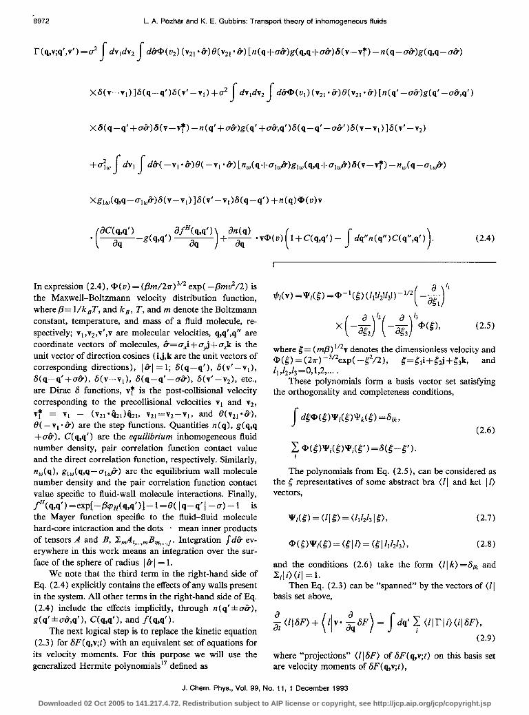
L. A. Pozhar and K. E. Gubbins: Transport theory of inhomogeneous fluids
xS(v-v,)]S(q-q’)S(v’-VI)+2 s ’ 4
dv dv d+D(ul)(v2,*&)~(vZ1*8)[n(q’--a&)g(q’-u&q’)
xS(q-q’+aWS(v-v:) -n(q’+aag(q’+a&,q’)6(q-q’--o&‘)S(v-v~)]6(v’-v2)
+do dv, s s W -vl*k)W -VI l G) [n,(s+al~)gl,(q,q+ul~~~(v-vr) -n,(q-aI>)
%%A%q--lum~(v-vl) NV’-v*)G(q-q’) +n(q)*(v)v
~fHbl’) -g(wl’) aq (2.4)
In expression (2.4), Q(U) = (f?m/2n)3’2 exp( -pmu2/2) is the Maxwell-Boltzmann velocity distribution function, where p= l/kBT, and kg, T, and m denote the Boltzmann constant, temperature, and mass of a fluid molecule, re- spectively; v1 ,v2 ,v’,v are molecular velocities, q,q’,q” are coordinate vectors of molecules, B=u,i+o,j +a& is the unit vector of direction cosines (i,j,k are the unit vectors of corresponding directions), I&I =l; 6(q-q’), 6(v’-vI), S(q-q’+a&), S(v-vl), S(q-q’-&), S(v’-v2), etc., are Dirac S functions, v;” is the post-collisional velocity corresponding to the precollisional velocities v1 and v2, 71 *= Vl - (v~1*ii21)(i21, VZI=VZ-~1, and B(vzI*B), 0( -vl * &) are the step functions. Quantities n(q), g(q,q +a&), C( q,q’) are the equilibrium inhomogeneous fluid number density, pair correlation function contact value and the direct correlation function, respectively. Similarly, n,(q), gl,(q,q--a,$) are the equilibrium wall molecule number density and the pair correlation function contact value specific to fluid-wall molecule interactions. Finally, fH(q,q’)=exp[-~~H(q,q’)l-11=8( Iq-d/ -d-l is
the Mayer function specific to the fluid-fluid molecule hard-core interaction and the dots * mean inner products of tensors A and B, 8~i ,..., ,B, ,..., j. Integration sd& ev- erywhere in this work means an integration over the sur- face of the sphere of radius I B I = 1.
We note that the third term in the right-hand side of Eq. (2.4) explicitly contains the effects of any walls present in the system. All other terms in the right-hand side of Eq. (2.4) include the effects implicitly, through n(q’ f a&),
g(q’*&q’), C(q,q’), and f(w’).
The next logical step is to replace the kinetic equation (2.3) for SF(q,v;t) with an equivalent set of equations for
its velocity moments. For this purpose we will use the generalized Hermite polynomials” defined as
I l++(v) =Y,(g) =w’(g>(1,!12!13!)- l/2
a 4 ( 1 -zT
x (--&)“( -&)bW, (2.5)
where g= (mp) “‘v denotes the dimensionless velocity and Q(5) = (2p)-3’2exp( -c2/2), ~=~Ii+~~+~3k, and li,I2,Is=O,l,2 ,... G
These polynomials form a basis vector set satisfying the orthogonality and completeness conditions,
r d@‘(SWAS)‘J’k(E) =61/c, J (2.6)
The polynomials from Eq. (2.5)) can be considered as the c representatives of some abstract bra (11 and ket 11) vectors,
VI(g) = (II@ = (I+,& 1 g>, (2.7)
*(c)y,(g) = (SI I> = (gl z11213>, (2.8)
and the conditions (2.6) take the form (I I k) =slk and EiIi)(il =l.
Then Eq. (2.3) can be “spanned” by the vectors of (II basis set above,
&(IISF)+(Ilv*~SF)=Sdq’~(llrli)(ilSF),
(2.9)
where “projections” (II SF) of SF(q,v;t) on this basis set are velocity moments of SF(q,v;t),
J. Chem. Phys., Vol. 99, No. 11, 1 December 1993
Downloaded 02 Oct 2005 to 141.217.4.72. Redistribution subject to AIP license or copyright, see http://jcp.aip.org/jcp/copyright.jsp
h I SF) = s dv$,(v)SF(q,v;t), (2.10)
and
(11~ $-F) = j-dv$,(v)v* $SF(q,v;t), (2.11)
dvdv’@(V’)$/(v)I’(q,v;q’,v’)+i(v’)*
(2.12)
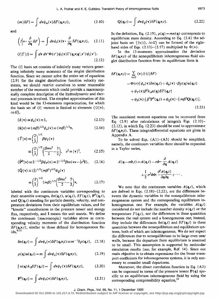
The (11 basis set consists of infinitely many vectors gener- ating infinitely many moments of the singlet distribution function. Since we cannot solve the entire set of equations (2.9) for the singlet distribution function velocity mo- ments, we should restrict ourselves to some reasonable number of the moments which could provide a macroscop- ically complete description of the hydrodynamic and ther- mal processes involved. The simplest approximation of this kind would be the 13-moments representation, for which the basis set of (II vectors is limited to elements { (iI v);
(2.13) The associated moment equations can be recovered from Eq. (2.9) after calculations of integrals Eqs. (2.10)-
(2.14) (2.12)) in which Eq. (2.23) should be used to approximate 6F( q,v;t) . These integrodifferential equations are given in Appendix A.
To be solved Eqs. (Al)-(A5) should be simplified, namely, the continuum variables there should be expanded
(2.15) in a Taylor series,
a (2.16) A(q--a&,t)=A(q,t)--a&* -&A(q,t)
+1(&.&.S+... . 2 * aqaq
(2.17)
labeled with the continuum variables corresponding to their ensemble averages, Sn(q,t), u(q,t), 6T(q,t), P’(q,t), and Q( q,l) standing for particle density, velocity, and tem- perature deviations from their equilibrium values, and for “kinetic” contributions to the pressure tensor and energy flux, respectively, and I means the unit matrix. We define the continuum (macroscopic) variables above as corre- sponding velocity moments of the distribution function SF(q,v;t), similar to those defined for homogeneous flu- ids 9-” t Mq,d = s dvtlt,(v)6F(q,v;t) =rn-‘bp(q,t), (2.18)
p(q)u(W) =m s dv$,(v)SF(q,v;t), (2.19)
$ n(q)kBST(q,t) = s dh4vPF(q,v;O, (2.20)
F’%A = s
dvrClp(vWYq,v;t), (2.21)
Q(u) = s
dv$,(v)SF(q,v;t). (2.22)
In the definition, Eq. (2.19)) p(q) = mn (q) corresponds to equilibrium mass density. According to Eq. (2.8) the ad- joint basis set {(v I i), ie G) can be formed of the right- hand sides of Eqs. (2.13)-(2.17) multiplied by Q(v).
In the 13-moments approximation the deviation GF(q,v;t) of the nonequilibrium inhomogeneous fluid sin- glet distribution function from its equilibrium form is
@Tq,v;Q = ,sG (v I i> (il SF) ‘Q(V) [$,(v)Sn(q,t) +$Jv) l &(q)u(q,t)
+$‘p(V):;p2p0(q,t) +$Q(V) l $ mD3Q(s,01. (2.23)
We note that the continuum variables A( q,t), which are defined in Eqs. (2.18)-(2.22), are the differences be- tween the dynamic variables in the nonequilibrium inho- mogeneous system and the corresponding equilibrium in- homogeneous one. For example, the variables A( q,t) considered do not include the number density n(q,t) or the temperature T( q,t), nor the differences in these quantities between the real system and a homogeneous one; instead, they include the differences Sn (q,t) and ST( q,t) in these quantities between the nonequilibrium and equilibrium sys- tems, both of which are inhomogeneous. We do not expect the differences due to nonequilibrium to be large even near walls, because the departure from equilibrium is assumed to be small. This assumption is supported by molecular simulation results (see, for example, Ref. 14). Since our main objective is to obtain expressions for the linear trans- port coefficients for inhomogeneous systems, it is only nec- essary to consider small departures.
Moreover, the direct correlation function in Eq. (A2) can be expressed in terms of the pressure tensor P(q) spe- cific to an equilibrium inhomogeneous fluid by using the corresponding compressibility equation,i8
L. A. Pozhar and K. E. Gubbins: Transport theory of inhomogeneous fluids 8973
J. Chem. Phys., Vol. 99, No. 11, 1 December 1993 Downloaded 02 Oct 2005 to 141.217.4.72. Redistribution subject to AIP license or copyright, see http://jcp.aip.org/jcp/copyright.jsp

8974 L. A. Pozhar and K. E. Gubbins: Transport theory of inhomogeneous fluids
Nq-4) C( WI’ I=
n(q) -&$/-$+iTr p(q,q’).
(2.24) where Sp(q)/Sn(q’) is the functional derivative of the equilibrium pressure p(q) =f Tr P(q) with respect to the equilibrium number density n( q’) taken at p=const, and
Tr p (q,q’) denotes the trace of the tensor p(q,q’). Thus, inserting the expression (2.24) for C(q,q’) into Eq. (A2), and taking time Fourier transforms of Eqs. (Al )-( A5), one can find expressions, correct to the second order in spatial gradients of the continuum variables (2.18)- (2.221,
au(w) CT4 -iioh(q,w) +$ . [n(q)u(q,w)] =--oh(q) JdSn(q-g&)g(q,q-&)(&&--i I): T+y n(q)
s d&n(q-&)g(q,q-&) (&&-g)& i aWq,d X aqaq +dfl(q)
X s d~n,(q-al~)gl,(q,q-u~~)~*u(q,w), (2.25)
a -iap(q)u(qJ) +& l
6p(q) dq’ Sn(q’) Sn(q’,w) -n(q)
s SP(fl”) 1
dq’dq” 8n(q’)hz(q’,o) -3s n(q) dq’ Tr p(q,q’)&z(q’,w)
1 +gj n(q) s dq’&“n(q”)Tr p(q”,q’)6n(q’,w))I+kBn(q)Wq,w)I+P”(q,w)l
s d~n(q--~)g(q,q--~)(~~-~ I)&?: a2u(q,w) 72 b2 aclag X77n(q) s d&n(q-m?)g(q,q--o&)
x (&&$ I)& auk4 -- (48flBr) ( ~)2bmp(q) I aq d~n,(cl-al~)gl,(cl,q-u,~) (@-a I) -u(w)
kBo4 +4 n(s) s d&n ( q - &>g ( q,q - CF.) &&& ~STh,d 3k& ah -4a 4s) s dan(q--3g(q,q
-a&)&&* amcw) as
a4 +T da) s d&g ( q,q - cr.) &&&&&: : a2p0(q,W) 3b
aqaq -G n(s) s
d&g(q,q-a&)&&&&i ap%d aq
4 2 +z II d&n(q)g(q,q-&)&&&+ ?
( 1s d~n,(s-ol~)sl,(a,a-u~~)~~ :P”(q,w) 1 +$$pb’w(d s d&g(q,q--a&) (&&-; I)&&; ~Q(s,d 36 B
aqaq -3; b2v(q) s dWq,q--&I
2 x (is-$ I)&: ach,d 24
aq +gPbv [s
d&[n(q)-n(q-&)]g(q,q-o&)(&f?--$I)-2V2
X s d~,(q-al~)g,,(q,q-u~~)(~~--P 1) l Q(q,w), 1 J. Chem. Phys., Vol. 99, No. 11, 1 December 1993
(2.26)
Downloaded 02 Oct 2005 to 141.217.4.72. Redistribution subject to AIP license or copyright, see http://jcp.aip.org/jcp/copyright.jsp

L. A. Pozhar and K. E. Gubbins: Transport theory of inhomogeneous fluids 8975
-io $ kgz(qW(q,wl+-& -Q(q,ol +kBT $ - [n(s)u(s,w)l 3ba
=G kBTn(q) d&n(q-&)g(q,q-m?)&&&i a2u(q,0) 3b auhd
aqaq -;?;; kBTn(q) d&n(q-cG)g(q,q-&)&c%: ~ aq
+&$JXq) s d^ un,(s-al~)gl,(ss-u,~~~*u(q,w) +$ b2An(q) s d&n(q-a&)g(q,q--o&)
XC% a*ST(q,w) 32bd?
ha9 --An(q) sd~n(q-~~)g(q,q-~~)~* 25lr asTjrti)+ [u4/(2 ml In(q) s dc?g(q,q-c+)
xfF&&&: aWqd
aqaq - (d/ J?rpm)n(q) s d&g(q,q-a&)&&i? apo~~“)+(c?/&) Jd&[n(q)-n(q-G)]
Xg(q,q-&)&& :PO(q,o) -gT n(q) I a*Q(q,w) 9b
d&(q,q-cG)&&&i aqaq -zg n(s) I d&g(q,q-o&)&% aQ(q,@)
84
302 +10 dG[n(q) +f n(a-03 lg(s,s-We+, d~n,(cl-al~)gl,(s,q-u,~)~ 1 l Q(q,wh
(2.27)
--i13wP”(s,w) +2S,,(q,w) +4 SQ(q,w)
a4 =y n(q) s d&n(q-a&)g(q,q-a&)(&&--f I)%+
a2uh44 ha4
-o%(q) sd&n(q- a&)g(q,q-o&) (cc-f I)&&
Wq,w) x~+2&P(s) s d~n,(q-al~)g,,(q,q-~~~) (&k-f I)B.u(q,o) +k B(&)lndn(q) sd&n(q-m?)
Xg(q,q-CT&) (is%-5 I)&& a2mwd aqaq -Zk,(&)lndn(q) s d&n(q-o&)g(q,q-h) (&h-f I)&* asTiTa)
+ ( &)“204n(d J di%g(q,q-o&) (&&-) I)&&&&: : aQ-%hd aqaq -2(&)“idn(q) Jd&g(q,q-c&)(&i+--fI)
X&&&i ap%,d
aq +2d(L)1'2[ J d&[n(q) -4n(q-m?)]g(q,q-&)(&h--f I)&&-3fl y ( )
2
CT4 a2Qh,d X s d~n,(q-a,~)gl,(q,q-~,~)(~~--f I)&& :P’(q,o) +y @z(q) 1 s d&g(q,q-&) (&h-j I)&&&; aqaq
-i d&(q) s d&g(q,q-&) (&F-f I)&&: aQ(q,o) 1
aq +5 ci$ d&[2n(q) -n(q-a&)]g(q,q-c&) (M-j I>&
d~n,(cl-al~)g,,(eq-u~~) (&e-i I)* .Q(a,w>, 1 (2.28)
J. Chem. Phys., Vol. 99, No. 11, 1 December 1993 Downloaded 02 Oct 2005 to 141.217.4.72. Redistribution subject to AIP license or copyright, see http://jcp.aip.org/jcp/copyright.jsp

8976 L. A. Pozhar and K. E. Gubbins: Transport theory of inhomogeneous fluids
5 kB a I a --iwQ(q,m) +- -- [n(q)ST(q,o)] +- - l P’(q,w> Wmaq Pm aq
ad%@) xg(q,q-~&)(a-~ I)& aq -- [V%J(B&%)ln(q) s d~,(q--ol~)gl,(q,q--al~) (&&
-3 1) l u(q,w) 3 kg4
+8 pm -n(q) d&z(q-o&)g(q,q-a&)&&& s
a2ST(q,w) 3 k&
ah ---n(q) dCn(q-o&)g(q,q-o&)&G
4 Bm s
asT(q,w) 3 CT4 +gpm 4s) s d&g(q,q--ui+)&&&&&: :
azPO(q,w) 3 a3 . as aqaq ----n(q) 4Pm s d&g(q,q-&)&&X+~ap~~)
102 +qFn s d~[3n(q)--2n(q--a~)lg(q,q-a~)~~~:P”(q,o) +g(Q4,\Ilr8m)n(q) Jd&(q,q-&)(&S--j I)&&;
~Q(w> 27 ’ acla<l -20 (d/ m)n(q) s di%g(q,q--h) (C&-i I)&
2
X dh[n(q) -n(q-c+)]g(q,q-&)(&&-$ I) -(52v2/27)
X d~n,(q-al~)g,,(q,q-~,~) (e-3 1) -$ s d~(q--~)g(q,q--~)(~+I) *Q(w). 1 (2.29)
In convolutions denoted by * , :, i, and : : on the right-hand sides of Eqs. (2.25)-(2.29) the right index of I in tensors I, I&, I&&, etc., are to be convoluted with the left index of the corresponding continuum variables, and indices &,&I%, etc., are to be convoluted with indices of a/aq, a2/aqiJq. In addition, quantities q= (5/162) (m/~-/3) 1’2 and A=75kJ [64&?rDm) 1’2] correspond to viscosity and thermal conductivity of a dilute gas. All other notations adopted in Eqs. (2.25)-(2.29) correspond to those introduced in Appendix A. Notations Sn(q,w), u(q,w), ST(q,w), P’(q,w), and Q(q,w) denote time Fourier transforms of corresponding continuum variables.
III. THE LINEARIZED NAVIER-STOKES EQUATIONS To obtain the linearized Navier-Stokes equation one should solve Eqs. (2.28) and (2.29), and insert the resulting
expressions for P’(q,w) and Q(q,w> into Eqs. (2.26) and (2.27). For this purpose Eqs. (2.28), (2.29) should be simplified. First, there are coupling terms of two kinds in Eqs. (2.28) and (2.29). The terms of the first kind are proportional to spatial derivatives sQ(q,a), aQ(q,w)/aq, and (#/aqaq)Q(q,w) in Eq. (2.28) and (a/as) l P’(q,o), aP’(q,o)/aq, and (a’/aqcYq>P’(q,w) in Eq. (2.29). If the temperature and velocity of the fluid do not vary appreciably in a mean free path ( -a) [which is valid in the case considered here, because continuum variables P’(q,o) and Q(q,w) are averaged quantities specific to a close-to-equilibrium fluid] the third order terms with the second derivatives of P’(q,w), Q(q,w>, and terms with sQ(q,a), and (Nag) l P’(q,w) in Eqs. (2.28) and (2.29) should be neglected.‘*” Moreover, since I o, I, I uv I, and / a, I < 1, the following conditions hold:
d&f (q-m?)-=; s d&[ f ( q-a&)-f (q+ch)v< J d&f (q-c+)- m= 1,3,..., i,j,k=x,y,z
(3.1)
d&f (q-o&)+ s d&f(q-c+)44>...> i,j,I=x,y,z, m=3,4 ,..,
for any integrable, positively defined function f(q), and m signifies that there are m a-components ai,...,Oj. Taking these relations into account one can prove that all terms with second derivatives of continuum variables in Eqs. (2.28) and (2.29) can be neglected. Finally, the derivatives (a/aq)P’(q,w) in Eq. (2.28) and (a/aq)Q(q,w) in Eq. (2.29), being small themselves, come with multipliers which are proportional to the integrals of odd sets of 2s over &. Then the correlation Eq. (3.1) and the simplest approximation
I d&f (q-*&)&..6z&
s d&f (q--c&)
I d&e.. .&
for the multipliers corresponding to these terms suggest neglect of these terms.
(3.3)
J. Chem. Phys., Vol. 99, No. 11, 1 December 1993
Downloaded 02 Oct 2005 to 141.217.4.72. Redistribution subject to AIP license or copyright, see http://jcp.aip.org/jcp/copyright.jsp
L. A. Pozhar and K. E. Gubbins: Transport theory of inhomogeneous fluids 8977
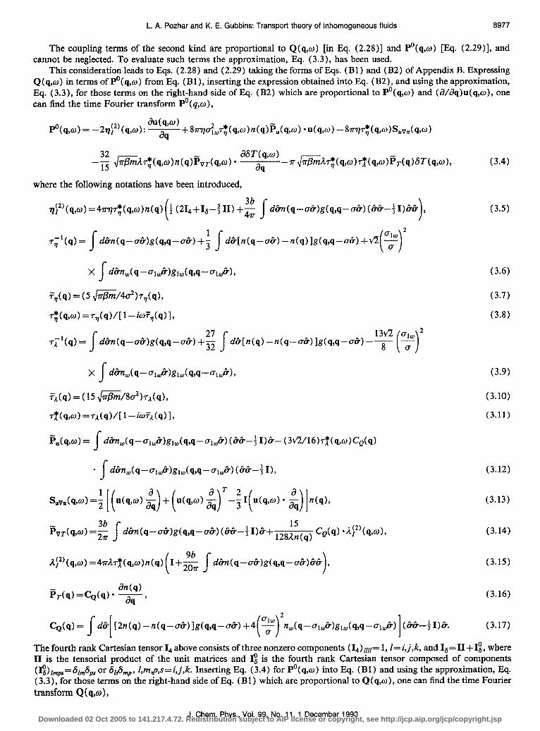
The coupling terms of the second kind are proportional to Q(q,o) [in Eq. (2.28)] and P’(q,w) [Eq. (2.29)], and cannot be neglected. To evaluate such terms the approximation, Eq. (3.3), has been used.
This consideration leads to Eqs. (2.28) and (2.29) taking the forms of Eqs. (Bl ) and (B2) of Appendix B. Expressing Q( q,w ) in terms of Pc( q,w ) from Eq. (Bl ), inserting the expression obtained into Eq. (B2), and using the approximation, Eq. (3.3), for those terms on the right-hand side of Eq. (B2) which are proportional to P’(q,w) and (cVaq)u(q,w), one can find the time Fourier transform P”( q,w),
~h,4 = --2rl~*bl,w):
NW)
~+grrrl~,r~(q,w)n(q>ij,(q,w) *u(w) -8~r/r,*(q,wBuv,(q,w) aq
-Ir~~r~((/W)r~(q,w)~~(q)ST(q,w),
where the following notations have been introduced,
#)(q,d =4~<(q,dn(q) 1 ~214+IB-~ 111 +g s
d&n(q-oi%)g(q,q-&)(&&-$I)&&
d&n(q-&)g(q,q--8) +; s
2
d&[n(q--a&) -n(q)]g(q,q-cS)+fl
X dan,(q-al~)gl,(q,q-~,~), I
,. n II
~q(q) = (5 J;rB;;;/4d?hqW, $(q,o) =rq,(q)/[ 1 -io7Jq) 1, T:‘(q) = d&n(q-&)g(q,q-a%) +g diXn(q) -n(s--a&) lgtw--&I -7
x d~,(cl-al~)gl,(cr,q-~,~), s C(q) = (15 Jsn/8&r~(q>, <Ccl,~) =q(q)/[ 1 -iwFA(q)],
Fu(q@) = s d~n,(q-~l&gl,(q,q-cs&) (&&-3 I)&- (32/2/i6)+f(q,ti)cQ(q)
- Id~~(q--,a)gl,(q,n-ol8) W-f I),
suVm(q@)=~ [ (U(P,O) &) + (u(q,w) $)‘-i I(U(q,W) l $-In(q),
d&n(q-G)g(q,q-o&)(&i%-; I)&+ l28;:(q) cQ(d l $2’h @) , ,
(3.4)
(3.5)
(3.6)
(3.7)
(3.8)
(3.9)
(3.10)
(3.11)
(3.12)
(3.13)
(3.14)
A:*‘(q,o) =4rAfl(q,w)n(q) (I+; I d~(q-~~)g(q,q-~~)~~), (3.15)
an(q) h-(s) =cQ(d l 7 9
(3.16)
J I 2
CQ(q) = d& [2n(q) -n(q-a&)]g(q,q-m?) +4 y n,(q-o,&)g,,(q,q-a,,@) (&&-$I)&. ( 1 1 (3.17)
The fourth rank Cartesian tensor I4 above consists of three nonzero components ( 14) /[,[= 1, I= i, j,k, and Is= II + e, where II is the tensorial product of the unit matrices and 1: is the fourth rank Cartesian tensor composed of components (J.3h,=b&or 4$,, , I m,p,s=i,j,k. Inserting Eq. (3.4) for P”( q,o) into Eq. (Bl ) and using the approximation, Eq. (3.3), for those terms on the right-hand side of Eq. (B 1) which are proportional to Q( q,w), one can find the time Fourier transform Q (q,w ) ,
J. Chem. Phys., Vol. 99, No. 11, 1 December 1993 Downloaded 02 Oct 2005 to 141.217.4.72. Redistribution subject to AIP license or copyright, see http://jcp.aip.org/jcp/copyright.jsp
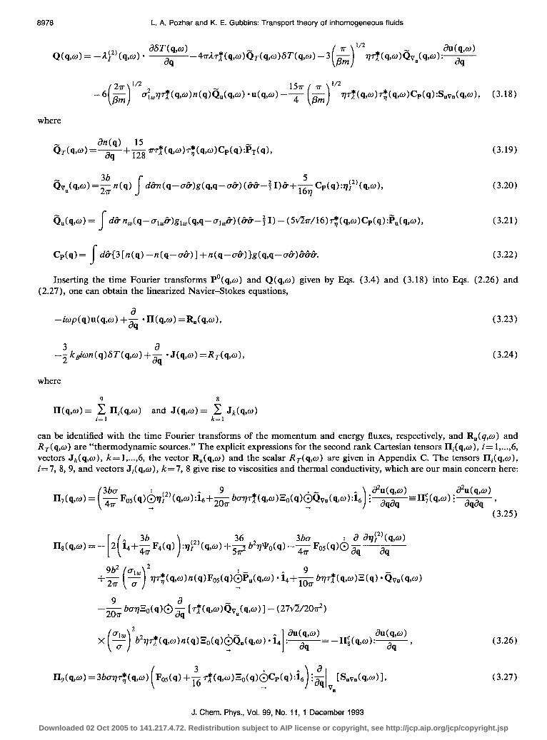
8978 L. A. Pozhar and K. E. Gubbins: Transport theory of inhomogeneous fluids
awq,w) l/2
Q(w) = -$2’(q,o> l aq -4rr;lTn*(cl,w)~T(q,O)ST(q,O) -3
aubd
rl~~t*(s,w)~!v,b&w):-
aq
l/2
71T~(cr,w)T~(cl,W)Cp(Q):Suvn(q,W), (3.18)
where
an(q) 15 ch+-w) =- aq += ?r7.~(q,w)T~(q,w)cP(q):~~(q), (3.19)
d&n(q-c&)g(q,q-o&) (H-i I)B+-5-- Cp(q):vj2)(q,w), 167
(3.20)
k(w) = j-d ~nn,(q-al~)gl,(q,q--ol~) W-3 I) - (5v%r/16)r;(q,w)C,(q):~,(q,o), (3.21)
Wq) = s d&{3[n(q) -n(q-c&)1 +n(q--k)}g(q,q---k)c%?. (3.22)
Inserting the time Fourier transforms P’(q,o) and Q(q,w) given by Eqs. (3.4) and (3.18) into Eqs. (2.26) and (2.27), one can obtain the linearized Navier-Stokes equations,
--iq(q)u(q,w) +$ l Wq,w) =RJw), (3.23)
-i kd~n(qRWq,w) +i *J(w) =RT(q,co), (3.24)
where
n(q,O)= ii1 ni(q,a) 8 and J(q,w)= c JAw) k=l
can be identified with the time Fourier transforms of the momentum and energy fluxes, respectively, and R,(q,w) and R r( q,o) are “thermodynamic sources.” The explicit expressions for the second rank Cartesian tensors l$(q,w), i= 1,...,6, vectors Jk(q,o), k= 1 ,...,6, the vector R,(q,w) and the scalar R.(q,w) are given in Appendix C. The tensors &(q,w), i= 7, 8, 9, and vectors Ji(q,O), k=7, 8 give rise to viscosities and thermal conductivity, which are our main concern here:
=II;(q,co, i aUq,d
a4aq f (3.25)
: a aq:2+q,w) :q:2bw) +; b2@,,(q) -; Fo5(q)@,, aq
77T~(cl,w)n(s)Fos(q)~~“(q,~) l i4+gr bvTf(s,w)E(q) l &Jq,w)
-gT b~~o(q)O f [~mMvy(q9w) I- (27fl/2/20$)
2 b277~~(q,w)n(q)~o(q)~~!u(q,o)‘i :dq= 1 h(q,o) h(q,w) -rI;(q,w):- aq 9
Edqm) =3bov;(qd Fos(q) +A +(q,m)EO(q)&4q):i6 [S”VdW) 17 1J” (3.26)
(3.27)
J. Chem. Phys., Vol. 99, No. 11, 1 December 1993
Downloaded 02 Oct 2005 to 141.217.4.72. Redistribution subject to AIP license or copyright, see http://jcp.aip.org/jcp/copyright.jsp

L. A. Pozhar and K. E. Gubbins: Transport theory of inhomogeneous fluids 8979
JdQ@) = - I( ‘+;TF2(9) #‘(q,w) +~h&(q) -gr F&q)6 aA12’( q 0) aq ’
-; bgAFw(q)h a [7,*(q,w)n(q)fivT(q,w>l-; b~~~~(q,o)~(q,o)F,(q)~~=(q) .I . -+ a4 1 amq,w) dq
=-J;GwP amq,o) aq , (3.28)
f Fodd&:2’(w4 l i4+8~~(q,w)n(q)F~(q)~~~~(q,~) . i, a2wwd a2~wl,~) aqaq = -J;(q,w): aqaq *
(3.29)
All new notations in Eqs. (3.25)-( 3.29) have been defined in Appendixes C and D. The continuity equation is considered in Appendix E.
A. Transport coefficients We now introduce the vorticity tensor W( q,w),
Then auk4 -=S(s,o) +W(q,o) +; I $ .u(q,o) aq
(3.30)
(3.31)
and
$1 am 1 [S,v,(%@) I=; S(S@) - ( aa) T 1 aq +Tj S(w) - VN a4 ) am 1 -Jj w(q,w) as ( am T --Yj W(q,o) q-
)
am 1 an(q) - - aq +T aq
where the transpose [AIT of the kth rank tensor A is defined as {A}~,.,m~Am,,,ji. Using expressions (3.30)-( 3.32) and (3.25)-(3.27) one can represent contributions II”(q,o) of the terms which are proportional to ($/aqaq)u(q,o) into (a/aq) l II (q,w) in the form,
a a n"(w) = -@j(w) '& s(q@) -+ml,d i& W(q,w) -hw) . $ (; .ukI,w)), (3.33)
where the fourth rank shear viscosity tensor fi (q,w) is 1 : II a : A 4(w) =z Kgs, d?l,--aq ’ n $ (%a) -%-W)?% , 1
the fourth rank turbulent viscosity tensor \jt(q,w) has the form
(3.34)
\iy(q,o) =n;(q& -’ l I$(q,@)+G2(q,&&, 1 6 as 1 (3.35)
and the second rank bulk viscosity tensor is defined as
i&w) =f (l$(q,w):I)@I- I 1
(3.36)
In expressions (3.34)-( 3.36), a1 denotes a convolution over the first left index of a tensor to the left of a1 and the index of d/aq from the expression (3.33), which should be performed after inserting expressions (3.34)-(3.36) into Eq. (3.33),
J. Chem. Phys., Vol. 99, No. 11, 1 December 1993 Downloaded 02 Oct 2005 to 141.217.4.72. Redistribution subject to AIP license or copyright, see http://jcp.aip.org/jcp/copyright.jsp

8980 L. A. Pozhar and K. E. Gubbins: Transport theory of inhomogeneous fluids
and dots over the symbol @i mean inner products. Moreover, convolutions in the large parentheses brackets in Eq. (3.36) and everywhere below should be performed first, and tensors Gi (q,w), G2 (q,w), and G3 (q,w) are defined as
Gdq,d=3bw;(q,w) I( an(q) Fos(q). -
aq -; GA4 +; $(q,o) Gdq) -; Gc(q)
an(q) 9 - FfE fl(q,w) an(q) 1 =o(s)ocP(cl):~ I-3 I GA(q) =Fodd$~ l i,),
an(q) ag ‘L Wq) =E,(s)~G(s):Il ry l i,), (3.42)
(3.37)
(3.38)
(3.41)
where the symbols Or and @i, denote convolutions over an index of the tensor to the left of a1 or ai, with an index of I or &, respectively. Although the turbulent viscosity tensor fi(q,w) from Eq. (3.35) is nonzero itself, the convolution \i(r (q,m) i (iVdq) W (q,w) is of the third order and should be neglected. Similarly, from expressions (3.28) and (3.29) one can obtain contributions J”(q,w) to (LVaq) . J(q,o) from the terms which are proportional to (c?/aqdq)6T(q,w),
J”(q,w) = -&q,o): a2mwd ata ’ (3.43)
where the second rank thermal conductivity tensor fi(q,w) has the form
;z(q,w) =J;(q,m)&t$ l J;(q,o). 1
(3.44)
Although expressions (3.34)-( 3.36) and (3.44) for viscosity tensors and tensorial thermal conductivity, respectively, have a complicated structure, they can be reduced to reasonably simple forms which can be proved to generalize those for the corresponding homogeneous fluid transport coefficients. This is further discussed in Sec. IV.
IV. ANALYSIS OF RESULTS
With some additional and not very strong restrictions the linearized Navier-Stokes equations (3.23) and (3.24) and expressions for the transport coefficients (3.34), (3.36), and (3.44) obtained can be dramatically simplified.
We assume now that the fluid inhomogeneity is due to the fluid-wall potential, and that no other external fields are present. This case would include simple fluids confined in capillary pores whose walls are composed of simple atoms (for instance, carbon, silicon, zeolites, etc.). Then from correlations (3.1) and (3.2)) it follows that in each set of terms in Eqs. (3.23) and (3.24) proportional to constants, h(q), and b2n2(q), one can restrict consideration to terms of tensoriality &%& in Eq. (3.23) and &% in Eq. (3.24), and among those terms for any integrable, positively defined function f(q) there would hold hierarchies of
j-d&f (q--3+$ f d&f (s-cW+w, s#I,
and
I d&f (q-c&)cf,
s d&f (q-&)apl, s#I, p,s,l=i,j,k.
Thus, for small u(q,o) and ST(q,w), Eqs. (3.23) and (3.24) take the forms
d~,(cl-a,~)gl,(cl,q-~,~)(~ I-66) l u(q,o), (4.1)
J. Chem. Phys., Vol. 99, No. 11, 1 December 1993
Downloaded 02 Oct 2005 to 141.217.4.72. Redistribution subject to AIP license or copyright, see http://jcp.aip.org/jcp/copyright.jsp

L. A. Pozhar and K. E. Gubbins: Transport theory of inhomogeneous fluids 8981
-$ iwkBn(q)ST(q,w) +a .P(q,o) =o, 84 where
n(q)I+$(q) an(q)
-~@&~(q,w)~;(q,o)Cn(9). ag
(4.2)
-; (Wh&)br/f+w)E(q) an(q) 72
l , ,+&b2Wo(s):
+~T8b~[B(q) l ~12’(q,~)lT ST(qw)-- ~k~~,,(q)+~b~~~(q,o)n(q) sd&n(q 1 ’ 1
+&Jb2h~(q,o)Z,(q)~ - an(q) I amw 48db
I aq aq 7 *(cl) +8rd, T;(q,w)n(q) s d+Uq
--al~)gl,(q,q--o,~)(~~-~ 1)6+4mh,*(q,w)n(q) A(q):; (214+IG---; II) I
1 1 I OI -u(q,o)
-8v<(wd i,+; F,(q) :f%v,(q,o) -%j”(q,o):s(q,o) -k”(q,o) $ l u(q,o), ( ) (4.3)
and
Jo(q,w) =f n(dI+E Q2(q) - ) d~n,(q-o,~)sl,(s,s-u~~) (ix%-; I) 1 l u(q,w)
+ gr bdA’%(q) -4rA?j:(w) I+gT F,(q) 1 ( am 63-r
l F+r ~~f!Ya,~)n(q)Wq) ST(q,w) 1 -LO( q,w ) l
am344 aq ’
(4.4)
and where the transport coefficients are given by
4o(q,w) =-w(q) [ 4r$(q,w) (it+: J d&z(q--&)g(q,q--&)(&%%%) ):(&+g J- d&‘n(q-&‘)g(q,q-&‘)
~((&‘&+?‘&‘~)+;b”I d~~(q--~)g(q,q--~)(~~~~) , 1 (4.5)
]iio(q,o) =v(d (2b$(w) s d Bn(q-&)g(q,q-c+)((&&)--jI)+;b2
x s d&n(q-r+)g(q,q--a%) [ (&+)-~(#*I,)] )
,
L0~q,w)=ln(q)[4~~(q,a)(I+~ Idn(q~~)g(q,q-~~~(~~)):(~+~ sdk’ntq-c@)
xg(q,q-o&‘)(cW))+$b2~d&n(q-&)g(q,q-&)(&)].
J. Chem. Phys., Vol. 99, No. 11, 1 December 1993
(4.6)
(4.7)
Downloaded 02 Oct 2005 to 141.217.4.72. Redistribution subject to AIP license or copyright, see http://jcp.aip.org/jcp/copyright.jsp
A. Transport coefficients in immediate vicinity of structured solid walls
8982 L. A. Pozhar and K. E. Gubbins: Transport theory of inhomogeneous fluids
In expressions (4.5)-(4.7) tensors (&&I%) and (&?) are those iX%&& and &&, respectively, in which components qmvm and WL with odd powers of indices p,s,l,m =i, j,k (e.g., ~Uj, ajO~, etc.) have been neglected, be- cause of hierarchies established at the beginning of this section.
As can be ea:ily seen from Eqs. (4.5)-(4.7), the ratios 4°(s,w)/n(a), ~(w>/n(s>, and L’(q,w)/n(s) do not depend on local values of the number density n(q). Simi- larly to the transport coefficients for the general case de- fined by Eqs. (3.34), (3.36), and (3.44), those from Eqs. (4.5)-(4.7) depend on position q and frequency w. The zero-frequency (or long time) limits of expressions (3.34), (3.36), and (3.44), or Eqs. (4.5)-(4.7) provide tensorial transport coefficients for the general case of inhomoge- neous fluids in time-independent external fields and/or in the presence of structured solid walls.
The general form of the relation between the number density and transport coefficients (or so called “smoothing procedure”“2) is Jd&n(q-u&)g(q,q-uC)&&&&. More- over, as can be seen from Eqs. (3.34), (3.36), (3.44), or (4.5)-(4.7), there are two of its reductions involved:
s d&n(q-u&)g(q,q-u&)6-&
= s
d&n(q-u&)g(q,q-a&)&&(&.&),
s d&n(q-u&)g(q,q-u&)
= s d~n(q-u~)g(q,q-u~)(6.8)(8*B).
Additional smoothing procedures appear in the general case of Eqs. (3.34)-(3.36) and (3.44), and are
s d&n(q-&)g(q,q-&)e
k and
Although, in general, there exists a variety of contri- butions to the transport coefficients, Eqs. (3.34), (3.36), and (3.44), caused by the presence of walls, the main con- tributions caused by hard-core fluid-wall intermolecular in- teractions are those which contribute to $(q,w) and fl(q,o) [Eqs. (3.8) and (3.11), respectively; at the zero frequency limit the 7*‘s are reduced to TV(q) and TA(q) defined by Eqs. (3.6) and (3.9)]. This fact becomes even more obvious after natural reduction of the transport co- efficients to those of Fqs. (4.5 )-(4.7), which assume no external field other than that of the fluid-wall interactions (see the beginning of this section). Quantities TV(q) and TA(q) are multipliers in the expressions for the main con- tributions to the shear viscosity and thermal conductivity tensors for all cases, including those for homogeneous flu- ids. As follows from expressions (3.6) and (3.9), the con- tributions to TV(q) and Tn(q) caused by hard-core fluid- wall intermolecular interactions are proportional to Sd~,(q-ul~)g,,(q,q-u~~), and are nonzero only for distances I from the walls which are about uu,,.
However, for separations Iz=(T,~ the values of r9(q) and Tn(q) can differ significantly from those for I> ulW Since both functions n,(q--a,$) and gi,(q,q--a,>) are positively defined, Jd&n,(q-ual$)gl,(q,q-u&)>O, and values of TV(q) at I~ui,,, could be smaller than those at I> ulW This could lead to a decrease of shear (and bulk) viscosities at distances Izu,~ from the walls. Moreover, from Eq. (3.6) it can be seen that the larger the ratio (at Ju) 2 is, the larger is such a decrease. Macroscopically, for walls of simple geometries this could result in sliding of the fluid monolayer nearest to a wall along the wall. This phenomenon (known as a slip in velocity) has been dis- covered theoretically” and confirmed by different experi- mental investigations in fluid mechanics (for example, in the case of a flow of hard spherical colloid particles in cylindrical channels16), and by computer simulations of low density gas flo~s~‘~~t and flows of simple liquids.22 Here we have provided a possible microscopic justification for these observations.
d&g(q,q-u&)&>, k= l,..., 5. k
In the case of shear viscosity, bulk viscosity, and thermal conductivity defined by J2q.s. (4.5)-(4.7), the reductions of the main smoothing procedure are
s d&n(q-u&)g(q,q-u&)ofd
and
s d&n(q-u&)g(q,q-u&)o$, I,s,p=i,j,k,
respectively. In the following subsections we consider several special cases of the further simplification of expres- sions (4.5)-(4.7) for the transport coefficients.
For the thermal conductivity the situation is quite dif- ferent. The hard-core, fluid-wall intermolecular interaction contribution to 7;3( q) is negative [see Eq. (3.9)], which can lead to an increase in the thermal conductivity of a fluid at distances IzulU from the walls. Once again, the value of this increase is defined by the ratio ( u,Ju)~, as well as by Sd~,(q-u,~)g,,(q,q-a,~). Quantities TV(q) and rL( q) are related to characteristic times TV(q) and Tn( q) of the momentum and energy redistribution responses of a fluid by relations (3.7) and (3.10), respectively. Thus, the results obtained show that in the immediate vicinity of walls the hard-core, fluid-wall intermolecular interactions accelerate the momentum redistribution into a direction normal to the walls, and do not effect significantly the tangential momentum redistributions. In addition, these interactions slow down the energy redistribution.
J. Chem. Phys., Vol. 99, No. 11, 1 December 1993
Downloaded 02 Oct 2005 to 141.217.4.72. Redistribution subject to AIP license or copyright, see http://jcp.aip.org/jcp/copyright.jsp

B. Dense homogeneous fluids
For homogeneous fluids the equilibrium number den- sities do not depend on molecular positions, n(q) =n, and g(q,q-&) =g(a). Subsequently, in the absence of solid walls, n,(q) =0, and the corresponding Navier-Stokes equations, which can be obtained from Eas. (3.23) and
L. A. Pozhar and K. E. Gubbins: Transport theory of inhomogeneous fluids 8983
and the fourth rank symmetrical Cartesian tensor T, has nonzero components as follows
4 (T,h=j T, I=i,j,k,
(4.17) 4 4A
(T,),,=~J p %dqr p,w,s=j,j,k. 1 $q4s
(4.8) Scalar shear viscosity &Jw) and thermal conductivity /z&(w) coefficients can be obtained by calculating the con-
(j.24) or (4.1) and (4.2), take the forms *
-hpu(q,o) _l_a l rI,(q,w) =o, as
(4.9) volutions &(w):S(q,w) and i!&(w). (a/aq)ST(q,o), in Eqs. (4.10) and (4.11), respectively,
ii~(~):ww) =&&m(q,4, (4.18)
i;(w) l d ST(q,w) =/z;Jw) d GT(q,w), aq as
(4.19)
where
-t ik@ntX’(q,w) +& l J&q,a) =0,
where
&f(w) =I I( )
dp Q(w) aP s +nkd 1 +nbg(a) I~~(%~) 1 ^O a
--2&b):Sh,d -K"g -u(q,o),
and Jdq,w) =nkA 1 +nbg(o) lu(q,w)
& [1+3n&W12
(4.10) (4.20)
and
and where tensorial viscosities +jL( w ), sH( w ) and thermal conductivity fig(o) do not depend on position q in the fluid, and are reductions of those of Eqs. (3.34), (3.36), and (3.44), or those defined by Eqs. (4.5)-(4.7):
AoH, =A (1 --io?,)-’ (4.11)
( $) [l+wxw12
+gr n2b2g(a) . 1
(4.21)
The scalar bulk viscosity p,,,( w ) follows directly from Eq. (4.13),
@H,,(w) =gv n2b2g(dq. (4.22)
Expressions (4.20)-(4.22) are identical to those obtained for dense homogeneous fluids in Ref. 11, and at the zero frequency limit lead to the familiar transport coefficients of
I 1
$&cd) =7j (1 -iGV)-’ - g(u)
i‘$+&nbg(u)Tq 11
: i,
+; &?(a) (T,--b n-11) +$ n2b2g(a)T, , 1 I g!J(w, =& n2b2g(a)$, (4.13)
;iO,(cd)=A (l-jfiFA)-’ i $j [l+Wgb)12
(4.12) dense homogeneous fluids. Similarly, substituting Eqs. (4.18) and (4.19) into Eqs. (4.10) and (4.11), one can recover Eqs. (3.14a) and (3.14b) of Ref. 11 for the Fourier time transforms of the momentum and energy fluxes, re- spectively, and the Navier-Stokes equations (3.13a) and (3.13b) of Ref. 11.
+& n2b2g( a) 1
I. (4.14) C. Fluids inhomogeneous in only one direction
In Eqs. (4.12)-( 4.14) the quantities ;i,, 7x are reduc- tions of those defined by Eqs. (3.7) and (3.10), respec- tively,
_ 5 rnfl ‘I2 5’16 q- ( 1
b&b) 1 -I, l5 mp “2[nc2g(o)] -I, “yz 7 ( i
We assume that the fluid is inhomogeneous only in the z direction. Assigning the origin of a spherical coordinate system (r&4> to position q=q$+q,j+q$=xi+yj +zk, so that 6 is an angle between the z direction and spherical radius r, and, thus o,=sin 6’ cos 4, a,,=sin 8 sin 4, and a,
(4.15) =cos 8, we can calculate the transport coefficient tensors (4.5)-(4.7) and derive explicit expressions for the terms -21i0bwasI,~), -K%,d wad ~uhd, and
(4.16) fi’(q,w) . (a/aq)ST(q,w) on the right-hand sides of Eqs. (4.3) and (4.4), respectively,
J. Chem. Phys., Vol. 99, No. 11, 1 December 1993 Downloaded 02 Oct 2005 to 141.217.4.72. Redistribution subject to AIP license or copyright, see http://jcp.aip.org/jcp/copyright.jsp

8984 L. A. Pozhar and K. E. Gubbins: Transport theory of inhomogeneous fluids
=2w(z) [.C,(w)S(w) +wwmd(q,~> +C3(z,~)~,(<l,~)I+C4(Z,O)S,(q,O)~kkl,
a&d $ •u(s,~)=~(w) $ l u(q,o)=~n(z)[K,(z,w)I+K2(z,w)~kkl; l u(q,w),
(4.23)
(4.24)
a ~“bl,w) l & fiT(w) =~“(z,o) l a GT(q,w) =AZn(z){i,(z,41+~2(z,co)ikk)* $ ST(q,w), aq (4.25)
where S,( q,w ) is the zz (or kk) component of the shear rate tensor S( q,w ), the second rank.tensor i,, has all components equal to zero but for the kk component which is equal to 1, and the second rank tensor &(q,W) is equal to the shear rate tensor S(q,w) in which components Sik(q,w), Ski(q,O), Sjk(qtO), and Skj(q,W) [or S,(q,o), S,(q,o), S,,(q,o), and S,(q,o), respectively] are set equal to zero. All other new notations in expressions (4.23)-(4.25) correspond to scalar quantities and are defined as
(4.26)
(4.27)
2+yx(z) +; a(z) -f g(z) [ 1+ (W4)x(z) 1 ww -t a(z) I [y(z) -$(z> -4 a(z) 1 W(z) -t a(z) 1 (4.28)
G(w) =6b[y(z) -p(z) -; a(z)] [r$z,o)(2+;a(z)+;y(z)-;@(z))+;b], (4.29)
Kl(z,w) =2b rr;(z,w) [x(z) -$ v(z) I+; &y(z) , I I
Kz(z,w) =2&-(z)
(4.30)
(4.31)
hw) =4m-f(z,w) 1 _t2 x(z) ( 20 )1 24 +25r b2x(z),
i2kd =F &,
(4.32)
(4.33)
where the quantities $(z,w) = r&)/[l - iwFV(z,o)] and fl(z,w) = rn(z)/[l - ~o?~(z,o)] [see ENS. (3.8) and (3.11), respectively] are reduced to T;(Z) = 7,&z) and e(z) = ~~(2) at the zero-frequency limit,
7$(z) =271- Y(Z) +f q(z) +v2 I
(4.34)
27 Y(Z) -5 q(z) - y ( 32v2tz)], (4.35)
s rr Yl (z) = &sin e[n(2-~c0se)-n(z)]g(z,z-~c0se), (4.36) 0
J- 7T
%3(z) = de sin enw(z--(Tlw cos e)glw(z,z-qw cos e), (4.37) 0 and
s
P a(z) = de sin’ eN(z,z--o c0s 13), (4.38) 0
J. Chem. Phys., Vol. 99, No. 11, 1 December 1993 Downloaded 02 Oct 2005 to 141.217.4.72. Redistribution subject to AIP license or copyright, see http://jcp.aip.org/jcp/copyright.jsp
L. A. Pozhar and K. E. Gubbins: Transport theory of inhomogeneous fluids
de sin3 8 ~0s~ eN(z,z- u cos e),
y(z) s Joffde sin 8 ~0s~ ehyz,z--a cos e),
!Az)= l ( dtl 2 sin 8 cos2 e-sin3 @N(z,z-ucos e),
I
lr x(z) = de sin3 eiv(z,z---a cos e),
0
s a
Y(Z) = de sin ejv(z,z-O cos e), 0
and where N(~,z-~ cos e) 52(~--~ cos e)g(z,z--a cos e).
In coordinate representation the Navier-Stokes equations (4.1) and (4.2) take the forms
(4.39)
(4.40)
(4.41)
(4.42)
(4.43)
(4.44)
271f3b4 $&(q,w) -jq+)q(q,w) + ( a *no(w) aq 1 -
=2#)(2,0) a S(qw) +2~j2)(z,w) 5s (q,o) I tap ’ 9 ), aq, a
-
+&ho) & (; .u(q,o)) +y $o( $j2W L$ vz(z) -x&z> -Lur(z)&ddq,~), I=f,j,k, ( corresponding to x,y,z, respectively),
(4.45)
-i jakBn(zMT(q,w) + i -
-J”(q,w) a2
=~Zn(z)L1(z,o)V2ST(q,w)+iln(z)2,(z,o) zGT(q,w), (4.46)
where
i l Il’?q,o))- and ($ l J’?q,w))- are divergences of the fluxes Eqs. (4.3) and (4.4), from which terms
: a -2ii0(s,d@ a(l W%@),
-P(q,u)?;iag ($ l u(wJ)), and
---;i”(q,d: & Wq,w), respectively, have been extracted; ul(q,w) is the I compo- nent of the velocity, 6,k is Kronecker’s delta, S,,( q,w) is the zi (or kl) component of the shear rate tensor, and L&(z) and xW(z) are defined by Eqs. (4.41) and (4.42), respec- tively, where N(z,z--a cos 0) has been changed to n,(z --(Tag cos e)g,,(z,z--o,, cos e).
In Eq. (4.45) the scalar shear viscosities, ~[s, and bulk viscosities K~(z,w)‘s are
rl11)(z,o)=77n(z)[C*(z,o)+(1--S~k)C2(Z,0)l, (4.47)
I
rlj2’(w) =vwCC3(w) + [C,(w) +c,cw)16~k), (4.48)
rlf3)(z,d =7p(z)C2(w) (alk- 11, (4.49)
KI(.w) =qn(z) [K,(w) +S~&(z,w)l, I=i,j,k. (4.50) The thermal conductivities in Eq. (4.46) are
A~(z,W)=An(z)2,(z,W) (4.51) and
j12(Z,O)=iln(z)Zz(z,w). (4.52) The transport coefficients (4.47)-(4.52) can be calculated immediately provided the equilibrium number density n (z) and pair correlation function contact values g(z,z --(T cos 0) are known for the composite potential pl.
Once again the transport coefficients for homogeneous fluids can be easily recovered from Eqs. (4.47)-(4.52). Indeed, for such fluids
$(z> -$ a(z) =o, C(z) =o, y(z) -PO(z) -: a(z) =o,
x(z) -$ Y(Z) =o, q(z) =o,
and v2(z) =xJz) =&Jz) =0 [since n,(z) =0], and one can derive
7jj2’(o) =?)j3’(w) =&(a) =L2(co) =o,
??j’b> =&&-J), A,(@) =$&4,
J. Chem. Phys., Vol. 99, No. 11, 1 December 1993 Downloaded 02 Oct 2005 to 141.217.4.72. Redistribution subject to AIP license or copyright, see http://jcp.aip.org/jcp/copyright.jsp

8986
and
L. A. Pozhar and K. E. Gubbins: Transport theory of inhomogeneous fluids
&b) =KoH,,w,
where &Jo>, n&(o), and pHsC( w) are defined by Eqs. (4.20)-(4.22), respectively, for all l=i, j, k.
In the particular case of a fluid in a narrow slit pore the results Eqs. (4.47)-(4.52), can be simplified further. We choose the z direction to be orthogonal to the pore walls, which are parallel to each other. Then the shear rate tensor will have just four nonzero components S,=S,, SyZ=Sry, because in a narrow pore of several molecular diameters width, u,( q,o) =O. As a result, Sd( q,w) =O. Subsequently, the right-hand side of the momentum conservation equa- tion (4.45) takes the form
sequently their dependence on q is not dramatic, it can still be significant. From a practical point of view it would be helpful to know for which specific inhomogeneous fluid systems, if any, the spatial dependence of the transport coefficients is negligibly small.
For this reason, we first consider the transport coeffi- cients in the case of external fields generated by fluid-wall intermolecular interactions only, Eqs. (4.5)-( 4.7). It’s clear that the ratios (transport coefficient)/n (q) would be independent of q if the quantities
ql,~), Tn*(%@>,
s d~(q--~)g(q,q--~)~~~,
xn(z> r: Y(Z) -x,(z) l~l(W), and
where 1=&j, and one finds a unique scalar shear viscosity coefficient
s d~~(q--~)g(q,q--~)~~,
s d&n(q-cG)g(q,q--&
~~lit~z~~~~~~~z~Cl~z~~~~ (4.53)
At the zero frequency limit it follows from Eqs. (4.53) and (4.26) that
are independent of q. In this case, since the spatial gradient of the number density of the equilibrium, inhomogeneous fluid is large, and, also, oi,oj,ak<l, one can expect that
a as s d~(q-~~)g(q,q-~~)o,~~~~9$ n(q),
mtW=vW am- (z) I+%‘( > 2+; b2$Czl LLz) I- (4.54) m,l,p,s=i,j,k
Similarly, the right-hand side of the energy conservation equation (4.46) is reduced to and, consequently,
Mz>[&,d +~2hdl &WwL (4.55)
so that the scalar thermal conductivity ~-slit(z) in the zero frequency limit is
asn(z)=iln(z)[Ll(z)+L2(z)l, (4.56)
where z,(z) and L,(z) are defined by Eqs. (4.32) and (4.33) and calculated at e(z,w) = TA(Z).
a
asl s d~(q-u~)g(q,q-u~)u~,o,($ n(s),
a
acl s d6-n(q--Wg(q,q-W -e$ n(s).
Moreover, from the definitions of the quantities rz( q,w) and e( q,w), Eqs. (3.8) and (3.11)) respectively, it follows from the condition
Other examples of fluid inhomogeneous in only one direction include fluids confined in narrow capillary pores of spherical and cylindrical geometries. The corresponding linearized Navier-Stokes equations and transport coeffi- cients can be found for these cases after rewriting Eqs. (4.45) and (4.46) in proper coordinate system representa- tions. We postpone investigation of such systems to our future work.
I d&n ( q - a&)g( q,q - a&) a,ap,o, z const,
that for distances larger than olw from the walls one can derive
$ [+pl,4 1 -I=$ [~n*h-l,d 1 -k$ 4s).
D. Inhomogeneity and the ratios (transport coefficient)/n(q)
As follows from the results obtained earlier, the trans- port coefficients, both in the general case [Eqs. (3.34), (3.36), and (3.44)] and in the case of external fields caused by the fluid-wall interactions only [Eqs. (4.5>-(4.7)], are functionally dependent on the position q in the fluid. Al- though the ratios (transport coefficient)/n(q) have been proved to be independent of local values of n(q), and con-
Indeed, these quantities depend on q through T,,(q) and 72(q), respectively. Then from Eqs. (3.6) and (3.9) one can show that for separations 1 q/ > on,, from walls the dependence of $ and r$ on q is defined by Jd&n(q - o&)g( q,q - oe), because of the inequality
I di+[n(q--a3 -n(q)lg(q,q--c+) 4 d&n(q-a&)g(q,q-a?). I
J. Chem. Phys., Vol. 99, No. 11, 1 December 1993 Downloaded 02 Oct 2005 to 141.217.4.72. Redistribution subject to AIP license or copyright, see http://jcp.aip.org/jcp/copyright.jsp

L. A. Pozhar and K. E. Gubbins: Transport theory of inhomogeneous fluids 8987
Consequently, we conclude that for inhomogeneous fluids for which sd&n (q - a&)g( q,q- a&> is almost independent of q, i.e.,
a
s
an(q)
as dh(q-&)g(q,q--h) Q-
aq 3 the ratios (transport coefficient)/n(q) will be almost inde- pendent of q as well. It can also be shown that this ine- quality is the necessary condition to have such ratios inde- pendent of q for the general case, Eqs. (3.34), (3.36), and (3.44). Noticing that
d&n(q-o&)g(q,q-o&)
= d~(q+Mg(q,q+&, s and recollecting that even for inhomogeneous fluids con- fined in narrow capillary pores of several molecular diam- eters width, the condition
I Gs 4s) ( -4: I-$ n(q) 1, w,p=i,j,k holds, one can expand n( q+a&) in the kernel of the inte- gral sd& n(q+o&)g(q,q+o&) in a Taylor series in o in the neighborhood of q. Restricting the series to the first three terms gives
w(q)+o c aj’) I=i,j,k
where
(4.57)
az= s d~g(q,q+ak), (4.58)
8(1), d~Ms,cr+a&, (4.59)
a(‘) = s
d&(Wg(q,q+&+), (4.60)
bo= d&n(q+o&)g(q,q+o&). s
(4.61)
In expression (4.57) we have neglected the contributions of op,, terms with Z#n into u(O), and assumed a2, a(‘), a(‘) to be independent of q. Although this additional restriction is not obvious in the particular case of external potentials generated by the fluid-wall interactions only, more detailed analysis shows that this condition is required to assure that the ratios (transport coefficient)/n(q) are independent of q in the general case [see Eqs. (3.34), (3.36), and (3&l)].
For a fluid inhomogeneous in only one direction (e.g., the z direction), Eq. (4.57) is reduced to
agz(z) +mp y+$g) qgLbo, (4.62)
where explicit expressions for u2, a:‘), and a:‘,
77 a2=2r
I de sin 6Jg(z,z+a cos f3), 0
a(‘)=297 s
IT z de sin 8 cos Bg(z,z+a cos f3), 0
57 p’=2~ .zz s
de sin 8 608~ eg(2,2+ o cos e), 0
(4.63)
(4.64)
(4.65)
can be derived from Eqs. (4.58)-(4.61) using a consider- ation similar to that in Sec. IV C, bo=v(z) [see Eq. (4.43)], and all notation correspond to those introduced in Sec. IV C.
If we choose the origin of the Cartesian coordinate system to lie somewhere inside a wall, than Eq. (4.62), as noted earlier, would hold for z-z,&r,J2 (the positive direction of the z axis corresponds to the direction from the wall into the fluid). Equation (4.62) is an inhomogeneous, linear, second-order differential equation, and at z>atJ2 +zW has the solution
where n(z) is a general solution of the corresponding ho- mogeneous equation, which, since quantities a2, al’), a$, and bo#O are real and positive, describes the damped har- monic space oscillator;23 for (a~‘))2-2u~)a2#0 it takes the form
RI(z) = I 0, z<z,+a1J2 CI exp[S~(z--z,--d2)1 +C2 exp[S2(z---Zw-qJ2)l, zZzw+alJ2
where C,, C2 denote constants, S,,, are
s*,2= -pi (p2--w;)“2, and where the damping constant p and the undamped natural circular frequency w. are
p--$& a
2a2 a;=-(. hz
(4.67)
(4.68)
(4.69)
(4.70)
J. Chem. Phys., Vol. 99, No. 11, 1 December 1993 Downloaded 02 Oct 2005 to 141.217.4.72. Redistribution subject to AIP license or copyright, see http://jcp.aip.org/jcp/copyright.jsp
8988 L. A. Pozhar and K. E. Gubbins: Transport theory of inhomogeneous fluids
At (a:'))* -2a~)a,=O the critically damped solution is
ii(z) = I
[Ct+C2(z-zZ,-oIw/2)]exp[ -p(z-z,-a&2)], z>z,+atw/2 (4.71)
0, z<z,+a*J2.
Since the relation (3.1) still holds, it is likely that for inhomogeneous fluids (u~~))*--~u~)u~ < 0 [see Eqs. (3.1) and (4.58)-(4.60)], and the solution (4.67) can be written as
I
0, z<zw+o~uJ2 ii(z) =
C3 exp[ -pL(z-z,--ad21 Isin[odz--z,--ad21 +a], z>z,+adJZ (4.72)
where the characteristic circular frequency UN iS
tij,,= (,;-p2)1’2. (4.73)
The constants Cl, C,, or C3 and cy in Eqs. (4.67), (4.71), and (4.72) should be chosen so that the solution K(z) defined by Eqs. (4.67), (4.71)) or (4.72) would satisfy the boundary conditions for the particular inhomogeneous fluid-wall system of interest.
The main conclusion of the discussion above is that for inhomogeneous fluids in which the equilibrium number densities n(q) behave qualitatively like damped spatial os- cillators one should expect the ratios (transport coefficient)/n( q) to be only weakly dependent on q. Sim- ulation data (for instance, Ref. 24) for the equilibrium number densities of fluids confined in narrow slit pores of width greater than 30 exhibit such damped oscillatory be- havior for n(q) .
The qualitative consideration above can be extended to inhomogeneous fluids in narrow capillary pores of cylin- drical and spherical geometries, which we will consider in the near future and, hopefully, to other systems of rela- tively simple geometries. Thus, we conclude that for inho- mogeneous fluids confined in pores of some simple geom- etries the ratios (transport coefficient)/n(q) should be only weakly dependent on q at separations from the walls ] qI > ald2. This conclusion is in a good agreement with that obtained by Davis and co-workers12’13724 from simula- tion data for velocity profiles of Couette flow in narrow slit pores of several molecular diameters in width. Though such fluids are strongly inhomogeneous, for strictly geo- metrical reasons the ratios (transport coefficient)/n (q) be- have as if the fluids are weakly inhomogeneous, and the corresponding Navier-Stokes equations are rather simple generalizations of those for homogeneous fluids.
V. CLOSING REMARKS
The transport theory derived above is a rigorous gen- eralization to inhomogeneous fluids of the Enskog-like ap- proach suggested by Sung and Dahler” for homogeneous fluids. Although rigorous this theory remains tractable, an advantage that derives from dividing the potential into hard-core and soft contributions. The transport coefficients thus derived have a simple and tractable structure, and can be easily investigated and evaluated. The theory incorpo- rates some approximations. The two basic ones are trun- cation of the set of moments equations and neglect of dy- namic memory.
I
The shortcomings of the 13-moments approximation can be alleviated, in principle, by expanding the basis set beyond the first 13 velocity moments of the singlet dy- namic distribution function. Although we do not have enough information on nonequilibrium inhomogeneous fluids to estimate the omission properly, it’s well known that for homogeneous fluids more accurate estimates of the transport coefficients at zero frequency in the conventional Chapman-Enskog procedure lead to slight modifications of the numerical values of the contributions proportional to n2b2g( a); these correction factors are ( 1.016) -’ for shear viscosity and ( 1.025) -’ for thermal conductivity.‘*” Thus, one does not expect the use of the 13-moments basis set truncation to lead to large errors. To correct this omission, one can use the Gross-Jackson ki- netic modeling procedure,25 which should be extended to inhomogeneous fluids.
The main contribution to dynamic memory effects is likely to come from repeated core collisions (not included in the theory presented here); there will also be smaller contributions due to the soft part of the potential. The neglect of these dynamic memory effects can be corrected for through analytic models, or by using molecular simu- lation data. Thus, one can make an approximate correction for these effects by adjusting the theoretical results to match simulation data for a fluid of hard spheres of the same hard sphere diameter, as has been done by Sung and Dahler, l1 who used Alder?6 and Dymond27 correction fac- tors. For inhomogeneous fluids the application of such ideas will be somewhat more complicated, since the density (and hence, the effective hard-core diameter, in the Weeks, Chandler, and Anderson (WCA) approximation discussed later) varies with position.
Calculations based on Eqs. (3.34), (3.36), (3.44), or (4.5)-( 4.7) require determination of the local equilibrium number density n(q), the hard-core diameter a, and eval- uation of contact values of the pair correlation function g( q,q- a&) for the intermolecular interaction potential pr of Eq. (2.1). The latter should be chosen so that it mimics some more realistic intermolecular potential, e.g., the Lennard-Jones model, pLT. To do this, one can use the Weeks, Chandler, and Anderson28 or Barker and Hender- son29 (BH) methods. Both methods have their pros and cons from the transport theory point of view. The WCA method supplies a hard-core diameter, u,,,, which de- pends on the equilibrium number density and temperature of the fluid, whereas the BH procedure yields a anu that
J. Chem. Phys., Vol. 99, No. 11, 1 December 1993
Downloaded 02 Oct 2005 to 141.217.4.72. Redistribution subject to AIP license or copyright, see http://jcp.aip.org/jcp/copyright.jsp
L. A. Pozhar and K. E. Gubbins: Transport theory of inhomogeneous fluids 8989
depends only on temperature. From a dynamical point of view there is scarcely any difference between collisional encounters described by potentials qI and Q)~, and it’s reasonable to take into account the averaged effects of such small differences in the potentials by choosing the hard- core diameter u to be a functional of density and temper- ature.“”
In using the WCA choice of hard-core diameter, we note that the theory incorporates an assumption that the hard-core diameter (T corresponding to local densities n(q) and n (q + 0 is the same, provided ( { 1 <a. We believe this may be a good approximation for many situations, since the density dependence of 0 is weak.28 Nevertheless, the theory should be regarded as a zero-order theory with re- spect to the density dependence of a, provided the WCA choice of hard-core diameter has been used. In order to avoid having to calculate o for every local value of n(q) it should be possible to introduce an averaged density n*, and then calculate owCA( n*).
The BH choice of hard-core diameter looks much more attractive for inhomogeneous fluids, because osH does not depend on the density of the fluid. In this case the theory developed above should be regarded as an exact theory with respect to the density dependence of o. How- ever, alleviation for the neglect of the dynamic memory may become more complicated, because it is no longer clear that the main contribution to the memory can be equated to those caused by the repeated hard-core colli- sions only.
The contact values of the pair correlation function g( q,q-&) can be obtained by direct computer simula- tions for a fluid with the intermolecular interaction poten- tial p’r of Eq. (2.1). Moreover, for homogeneous fluids Sung and Dahler” found that for the WCA choice of hard- core diameter the following correlation holds,
d”WCA) g(%J)
8dcWCH) “gH( ’ (5.1)
where gH( oLT) and g& owo.& are the contact values of the pair correlation functions specific to the hard sphere fluids with hard sphere diameters equated to o, (where o, is the Lennard-Jones parameter) and owoA, respectively, and g(a,) and g(owCA) are the contact values of the pair-correlation functions for the Lennard-Jones fluid. Similar correlation may hold for the corresponding local contact values of the pair correlation functions in the case of inhomogeneous fluids, and this could lead to a reason- able approximation of g(q,q-o&) specific to the compos- ite potential rpr.
Finally, we note that at the simplest level one can es- timate the quantities
s d~n(q--~)g(q,q--~)(~~~~)
and
s d& n(q-&)g(q,q-m?) (6%
in Eqs. (4.5)-(4.7) heuristically, as was done in Ref. 1 for a fluid inhomogeneous in only one direction. While such an approach may give immediate results, it will be of uncer- tain validity and likely to break down in unforseen ways. We plan to test the theoretical expressions for the transport coefficients presented here via molecular simula- tions for fluids near walls and confined within pores, and these results will be presented in future papers.
ACKNOWLEDGMENTS
It is a pleasure to thank H. T. Davis for useful discus- sions. This work was supported by grants from the Na- tional Science Foundation (Grant No. CTS 9 122460) and by a contract from the Gas Research Institute (Contract No. 5086-260-1254). L.A.P. thanks the Materials Science Center and the Center for Applied Mathematics at Cornell University for support as a Visiting Scientist at Cornell.
APPENDIX A: INTEGRODIFFERENTIAL FORM OF THE MOMENT EQUATIONS
The integrodifferential equations obtained by using the 13-moments approximation are
i 6n(q,f) +$ - [n(qh(eO 1 =&t-d s dih(q--c?)g(q,q--oC)6* [u(q-o+,t) -u(q,t)] +ofs(q)
X I d~n,(cl-a,~>g,,(cl,q-u*~)~*u(q,f),
& [p(du(q,t)l+$ l p(s,t)+kB$ l [n(q)sr(q,r)lI+~$sn(r,r)
=f Idq’[n(q)(dC(aqdq”-g(q,q’) afHiy’))+y (l+C(q,q’)- ~dp”n(q”)C(s”,4’))]Sn(q’,t)
den(q--i+)g(q,q--3 (CC-3 I) l [u(q-a&t> -u(q,t)] -2v%f, n(s)
(Al)
J. Chem. Phys., Vol. 99, No. 11, 1 December 1993 Downloaded 02 Oct 2005 to 141.217.4.72. Redistribution subject to AIP license or copyright, see http://jcp.aip.org/jcp/copyright.jsp
8990 L. A. Pozhar and K. E. Gubbins: Transport theory of inhomogeneous fluids
o% x d~,(q-al~)gl,(q,q-~,~) (E-3 I) l u(q,t) +T n(q) s dWq-&g(q,q--3
XB[ST(q-u&,t) --GT(q,r) ] +; s
d&g(q,q-a&)&&&[n(q)P”(q--a&J)--n(q--o&)P?q,t)]
2 s 40 +z d&n(q-o&)g(q,q-o&)&&&P”(q,t) +y s d~,(q--(Tl~)glw(q,q-~l~)~~~PO(q,t)
diig(q,q-cG) (&&--$ I) l [n(q)Q(q-a&J) -n(q--o8Q(W>l d~,(cl-a,~)s,,(<r,q-u,~) W-f I) l Q(q,t), (A21
2 k,n(q) & tWq,t) +$ l Q(q,d +kBT i l [n(aMs,d 1
a2 s
4ul =2p n(q) d&n(q-a&Mq,q--acTW [u(q-a&,[) -u(q,t) I +p n(q) d~,(q-al~)gl,(q,q-al~)B
l u(q,t) + (kB/~)$n(q) s dh(q- o&)g(q,q-ff&) [ST(q-a&t) --ST(qA I+ (4/&&a 302 x d&g(q,q-&) (&9-f I):[n(q)P’(q--a&J) -n(q--C)P’(q,t)] +F dbg(q,q-o&)8
l [n(q)Q(q-a~,t)-n(q--a~)Q(q,t)l +y s
d&n(q--&)g(q,q-oc%)B*Q(q,t)
+aTUJ s d~n,(q-al~)gl,(q,q-~,~)~.Q(q,t), (A3)
p & P”(q,t> +=,,(q,t) +; sQ(%t)
=&z(q) Sd~n(q-~~)g(q,q-~~)(~~-~I)~* [u(q-a&J)-u(q,t)]+2&n(q) ~d&n,(q-rrl$)
x&,(q,q--alu$)(&&-; I)cSu(q,t)+2k& !- ( Tm)1’2dd J d&n(q-o&)g(q,q-m%)(&&--fI)
x[ST(q-u~,r)-BT(q,f)l+2(~)1'2~ld~g(q,q- I( a& S-f I)&&:[n(q)P”(q-o&J) -n(q-a&)P”(q,t)]
-6(h)‘” j- c? d&n(q-h)g(q,q-m&)(&i%-$I)&&P’(q,t)-6fl B (~m)1’2~,~d~n,(q-rrlZ)
Xgl,(q,q--a,@)(&&--f I)&&P”(q,t) + ipc? s d&g(q,q-r.S) (i%&-~ I)&* [n(q>Q(q-a&J)
-n(q--a&)Q(q,t)] +ifldJd&n(q-m%)g(q,q-o&)(&C-iI)&*Q(q,t)
dk n,(q-a,~)g,,(q,q-a,~) W-f W*Q(W>, (A4)
J. Chem. Phys., Vol. 99, No. 11, 1 December 1993
Downloaded 02 Oct 2005 to 141.217.4.72. Redistribution subject to AIP license or copyright, see http://jcp.aip.org/jcp/copyright.jsp
L. A. Pozhar and K. E. Gubbins: Transport theory of inhomogeneous fluids 8991
&Q(P.f)+g$-$ [n(q)GT(q,r)]+&$ .PO(q,t)
=(d/28m)n(q) Jd&n(q- af?)g(q,q-m?) (is&-$ I) l [u(q-a&,t) -u(q,t)]
-(fi&/P&&>n(q) JdA 32 kB
u n,(s-al~)sl,(scl-al~) t&4 I> *u(w) +- - n(s) 4 Pm
x I d&n(q-c&)g(q,q-&)6[6T(q-u&,t) -GT(q,t) ] +-& I d~n(q--~)g(q,q--~)~~~:P’(q,t)
+g Jd&g(q,q-&)&&&[n(q)P”(q-&,f) -n(q-&)P’(q,f)] -(2$/S J?rpm) Jd&n(q--a%)
xg(q,q-03 (bti+I) *Q(w) + (27&20,/&d j- d&g(q,q--ok) (&F-$ I) l [n(q)Q(q--a&,f)
-ds-ui+)Q(s,t) I- (13fl&,/5 ,/$%I s dh n,(s-al~>gl,(sq-ol~) (kc-3 1) *Q(w). (A51
In Eqs. (Al )-( A5) I denotes the unit matrix, and quantities
A n a...u, n n=2,3,...
are the nth rank Cartesian tensorial products of the direction cosines vector B with itself; thus, for instance, &&&& is the fourth rank Cartesian tensor composed of 81 components (oiop,a,>, i,Z,m,s=x,y,z. Similarly, [cc--- ( l/3)1]&, [&&- ( 1/3)I’@&, etc. are tensorial products of the tensors [&&- (l/3)1] and B or &&. The second rank Cartesian tensors S,,(q,t) and S,(q,t) are defined as
Sm(q3f)=i $ [u(q,f)n(q) I+ $ b(q,f)n(q)] I ( T2 a
) ( -3 I ;r; l [u(q,f)n(q)]
)I ,
S,CW)=; [ (~Q(,,r,)+($a(,,t))T-~I($ *Q(s,r))l, (A61
(A7)
where C(a/aq)[u(s,f)n(q)l}T (a/aq)[Q(q,f)], respectively.
and {(a/aq)[Q(q,f)]}T denote the transposes of the tensors (d/aq)[u(q,f)n(q)] and
APPENDIX B: REDUCED EQUATIONS FOR P’(q,o) AND Q(q,w)
Reduced equations for the time Fourier transforms of the “kinetic” contributions to the energy flux and the pressure tensor are
-iwQ(q,w) + [82/15 ml [ s dti(q---CMq,q--h) +z s d&[n(q) -n(q-&)]g(q,q-oh) - (13vW8)
d~n,(cl-ol~)gl,(s,s-al~) Q(q,m) 1 = -2 -& [n(q)ST(q,w)] +F ~d&z(q-c&)g(q,q-&)&&*a’T~~‘m) - bwsV2P Jn;pml
X s h(<l,@) ~&m-4) d&n(q-o&)g(q,q-&)(&&-$I)&:----- aq -3GEd d~n,(q-o,~)g,,(q,q-o,~) W-; I)
2 x l u(q,o) +- Wm s d&[3n(q) -2n(q-&)]g(q,q-&)&6tkP”(q,w), (Bl)
J. Chem. Phys., Vol. 99, No. 11, 1 December 1993 Downloaded 02 Oct 2005 to 141.217.4.72. Redistribution subject to AIP license or copyright, see http://jcp.aip.org/jcp/copyright.jsp

8992 L A. Pozhar and K. E. Gubbins: Transport theory of inhomogeneous fluids
d -ioPO(q,o)+~S,.(ao)=-,n(s) s
MwJ) 2do d~n(q--~)g(q,q--~)(~~--;I)~~- - aq + p n(s)
x I d~n,(q--,~)g1,(q,q--,~) w-f IW*u(q,o) - cw6-J-v J;rBmMq)
s asmw
X d~n(q--~)g(q,q--~)(~~--51)6* aq - (402/5 J;ram>
(I
2
X d&n(q-a&)g(q,q-a&) +; J- d&g(q,q-CT&) [n(q-a&) -n(q)] +v2 ? ( )
s 1 l3 X de n,(s-al~)gl,(s,cl-al~) e-l44 +-J- IJ
d&[2n(q) -n(q-o&) ]
xg(q,q--o&) (&&-+ I)&+4 ? 2
( )J dC n,(s-a1~)g,,(s,cl-a1~)
x (&i?-f I>& l Q(q,o). 1 (B2)
If one assumes n(q) =const. n,(q) =0, and g(q,q-o&) =g(a), then from Eqs. (2.25)-(2.27) and Eqs. (Bl) and (B2), one can recover the 13-moments approximation equations for dense homogeneous (bulk) fluids.”
APPENDIX c: THE FIRST SIX CONTRIBUTIONS TO THE MOMENTUM AND ENERGY FLUXES, AND RJq,w), &&4
The explicit expressions for the first six contributions to the momentum flux lI(q,o) are
&(q,w) = SP(cl)
dq Sn(q’) ’ - Sn(cr’,o) -n(s) II- Sp(q”) 1
WW in Wq’,o) --a n(a) s dq’ Tr ~(q,q’)Wq’,~)
1 +3p n(q) ss
dq’dq”n(q”)Tr p(q”,q’Mn(q’,o) I, (Cl)
n(q)I+$%h) -~&=7;t(q,o)$(q,m) :&(q) +T ,/&&Fo5(q)b $
2
x lAYq,w)~sl(s,w)~,(q~ 1 -~w~~~hoEw l arbLw> +g A~~o~4~~ $[~h&O)~T(q.“) 1
16 +ij ~~Wd+-w) M(q):b(q,d I ‘+gT bo&[B(q) 4j2’(q,w)]’ ST(q,o), 1 (C2)
g k,*,,(q) +; &&A~(q,o)n(q) i,+g &(q):i, :hdw) -$ &?=m~Fc,dq)~;
x [~(q,w)n(9)~sr(cLo)l+~~PbblllBo ‘L:2’(q,o)-~Bb2?TBo(9)~ ap(q w) aq ’ awq,@)
+f ~~ff~?:(q,w)~(q,w)F,,(q)~Br(q)I+~~Bb2~~~(q,w)~,(q):~=(q,o)I l aq , 1 (C3)
J. Chem. Phys., Vol. 99, No. 11, 1 December 1993
Downloaded 02 Oct 2005 to 141.217.4.72. Redistribution subject to AIP license or copyright, see http://jcp.aip.org/jcp/copyright.jsp

L. A. Pozhar and K. E. Gubbins: Transport theory of inhomogeneous fluids 8993
I&(w) = ~~ff~~(q,o)n(q)F,,(q)~B,,(q,o) l i4+~gb2?a,(P)~)2)(q,o) l i, : a2aza;0) ,
)
(C4) -e
I 482
Wcl,@) = 5 WJ’(d +8~~,77~(s,o)n(q)~“(q,~) +6~917~~(s,o)n(s)Fh(q):B,(q,w) -3&,ob~Fo& $
x b-qs,wMs>P,(sw) I- (9~/5P)~9rl~(q,o)n(q)&(q) l a,cc& + (9vm0T)c7Qmjao(q)~ $
X [~(wMq)tbw) 1 +&W:~j2b-w) 1 ‘oI+; dr/~:(s,o) [B(q) &(q,4 101 1 *UC%@1, (C5)
&(w) = 1
-8rrr/<(q,d i,+; F Cd +3~q$+w)Fos(db ;I ( 4, II
il+3~ollFor(dO; [$(q,d 1
-f b-pci,~)G(a,~>~~~~ *C,(q) +; ba77~‘oWQ $ bpl,4~@w,01
9 +E ~~~~s,o,bcq,~~~.cq~~~~~~:~ i4 :S.vn(q,W).
1 I ” CC61
In expressions (Cl)-(C6) [D]r CPIT~
means the transpose of the pth rank Cartesian tensor D defined by the expression I,,,.,.~= Ds...,,,l, and an open dot (0) denotes a convolution over the second left index of a tensor to the left of 0 and
a regular index of the tensor to the right; notations @ and a+ denote convolutions over a $ index of a tensor to the left of the corresponding convolution sign and a (a/aq) index of a tensor to the right; in the case of a4 the (a/aq) index of a tensor to the right should be taken after executing convolutions of tensors i $. lj, or I with the corresponding continuum variable or its ;patial gradient. The sixth- and fourth-rank Cartesian tensors lg, l4 are composed of components ( 1,) lmnsPq =~1~mpL (14)Imm=Wmn9 respectively (S-S here are Kronecker symbols), and are considered in Appendix D. Gradi- ents (a/as) IU in Eq. (C6) and (mq) IVn in Eq. (3.27) are to be calculated at u(a,w) and Vn (a) fixed, resnectively, and V 3 (a/aq). All other new notations in l&s. (Cl )-( C6) are as follows: -.
-. a
@,(q)=n(q) d&n(q-&)g(q,q-cr&)u+gi . s I
d&n(q)n(q-&)g(q,q-&) m m+l
Fm(q)=n(q) I d&g(q,q-m.?)$...&+;; l
m I
d&n(q)g(q,q--a& m+l
=(q) =n(q) J d&(q,q-&)6(&i%-; I) +?a l
2 aq s d~(q)g(q,q--aci)~~(~~-~ I),
y(q) =n(q) I d&n(q-&)g(q,q-a&)&(&&-~ I) +za l
2 as d~(q)n(q-a~)g(q,q-a~)~~(~~-~I),
Fo,(q)=n(q) I d&g(q,q-cG)y M= 1,2,...
Qom(q)=n(q) s d&n(q-o&)g(q,q-pi+)-, m=1,2,...
m
(C7)
(C8)
(C9)
(ClO)
(Cl11
(Cl21
(C13)
(Cl4)
s(q) =n(q) s d&(q,q-ui+) (&St%-3 &I&),
Wd =&cl) I dh n(s- a&)g(q,q-ff&) (f%?&&-$ &I&),
d~n,(q--l~)gl,(q,q-ul~)~~~+ s d&in(q) -n(q-h)]g(q,q-mC+)&&&,
(Cl5)
J. Chem. Phys., Vol. 99, No. 11, 1 December 1993 Downloaded 02 Oct 2005 to 141.217.4.72. Redistribution subject to AIP license or copyright, see http://jcp.aip.org/jcp/copyright.jsp
8994 L. A. Pozhar and K. E. Gubbins: Transport theory of inhomogeneous fluids
a B(q) =uag l d& n(q)g(q,q--a&) (&k-i I)&+:$ 9 d&n(q)g(q,q-&)&(&S-f I)&
d&[n(q)-n(q-h)]g(q,q-a?)(&&-$I)-W2 d~,(s-ol~)gl,(q,cl-ul~) W-5 I).
(Cl61 The first six contributions to the energy flux J(q,w) are
Jl(q,w) =f n(q)I+g Q2(q) - (15vW8) (Tlw Tf(q,w)n(q) I+g F,(q) ) ( u )’ ( ) -Q,(d+W2/2/64~)
2boFo3(q)6 $ [ff(q,w)n(q)~!,(q,o)] +g 2
b~~(q,w)n(q)F3(q):~‘u(Q,w) 2 baFo4(q)b $ [~(so)n(q)f,(s,o) I+& [Uq):d2)(q,w) 1 T+A fl(q,w)
x [M(q) l &ubw) I= l u(cl,w), 1 (C17)
Jz(s,w) =; ; $hdWcl> +; o%dqEI; ~h,d -2 $ T;(q,w)G(q,w) I+gT F2(q) -C,(q)
+z ?ro2Fo& $ [~(s,d%w>C,(s) 1 :%n(w), 1 ((38)
J3(q,m) = (3ba/ J;rpm)rl 2+w)Fo&) +g ~.r;(q,+-f(q,4F03(q)6Cp(q):i, ii [S,vn(w) It (Cl91 Ja(q,w) = - (I/&%) $ v%(q) +; F3(q):v:2’(q,w) -g F&q)6 $ v:2’(q,4
2
-; b+ob $ bl%wdv,(q,w) 1 -z 1 au(q,d b2rl~(s,w)n(s)Fo3(q)~~~(q,~) -& :T,
cc201
Js(q,o) = (3bu/2 @6) iFo4(q)~ll:2’(q,o):ia+% 77~(q,o)Fo3(q)~~v”(q,~):i6 aWq44
aqaq 9 cc211
$ bgA@,(ci) -; bh$Yq,w)$(q,w)F3(q):&(q) -4de(q,w) I+;),(q) .&(q,o)
+; bdFdq)6$ [d(%~)~T(%a)l +E $il~(q,o)n(q)L(q):~VT(q,O) +i dM(d l $2%&d
+a bu-od& $ [+w)~(s,d&h-d 1 ) ST(w). ((32)
Here
L(cl)=o; e%(q)+ s d&[n(q) -n(q-a&)]g(q,q--a&)&& (CT31
and M(q) =u$ *b(q) + f dNn(q) -n(q--3 lg(q,q-o&b+: J- d&n(q-a&)g(q,q-c+)B
(C24)
J. Chem. Phys., Vol. 99, No. 11, 1 December 1993
Downloaded 02 Oct 2005 to 141.217.4.72. Redistribution subject to AIP license or copyright, see http://jcp.aip.org/jcp/copyright.jsp
L. A. Pozhar and K. E. Gubbins: Transport theory of inhomogeneous fluids 8995
The right-hand side of Eq. (3.23) takes the form
2
~o??=n*(wMci)B(d *ada@) +g o%($ l [Tf(q,wD(q) l &,(q,w) IT) ‘1 l u(q,w>
-‘% 4’-@dA(d +; ++-u4~~q,w>Wqr) .Cp(q) :SuVn(q,m) + ,/i&h I 1 gT h? $ . a2(q)
+g 2 i l [T~(q,o)n(q)A(q):iiivT(cr,o> 1 ‘--E 02~(cr,w>7~(q,w)A(q):~=(q)
a2a 4 +m g l [B(q) •~:2’(s,dl =-F c+fhdBW .&(q,d ST(q,w). 1
For the right-hand side of Fq. (3.24) one can derive
(C25)
R,(w)=; (;b; l Wq)+&dq) j-dA on,(q-al~)gl,(q,q-ul~)~+~ a - [L(qhp(q,w)] =+z a 83~ aq 32 aq
l [<(q,@)M(q) ‘%(q,@) ] T+G ~,~(q,o)n(q)L(q):~,(q,w) - (9~~16)&,~(q,w)n(q)M(q)
4swd 225~ 256 $hwMf(q,w)M(q) *G(q)
(
32b$ a +A -- 25~ aq *@l(q) -~~~(cl,W)Tn*(S,w)L(q):fjT(q) -f %-dfl(q,dM(q) l &-(q,d
+gd $ - [7~(ew)n(s>L(q>:Pv,(a,w)l +j$$ l [M(q) .nj2)(q,w>l )
ST(q,o). CC261
If n(q,w) and ST(q,ti) are sufficiently small (i.e., the system is close to an equilibfium state, as assumed) R,( q,w) and RT(q,w) are negligibly small, although an(q)/dq may be large, even of the order n(q)/o. In the immediate vicinity of walls the main contribution to R,( q,w ) would be that from the second term on the right-hand side of Eq. (~25); thus, for R,(q,w) and R,(q,w) one will have
48~7 R,(q,w) = -F bqn(q) (C27)
and
RT(%@) =o. (C28)
Thus, although due to the assumed immobility of the wall molecules there is momentum production in the system, this production is only noticeable in the immediate neighborhood of walls.
APPENDIX D: TENSORS i,
We define the 2mth rank tensors i,, so that
Ci2m),spl ,...,~2s212=sl,l~sS*S26p,4”” m= 1929”’
v- m
(Dl)
where the Sk’s are Kronecker symbols and II,sI,p1,...,p2,s2,12= 1 2 3 , , ,..., n. Then for any mth rank tensor A one can prove
i,,@A=A, (D2)
A@i2,=A, (D3) n 12m@i2m= i2m 9 (D4)
J. Chem. Phys., Vol. 99, No. 11, 1 December 1993 Downloaded 02 Oct 2005 to 141.217.4.72. Redistribution subject to AIP license or copyright, see http://jcp.aip.org/jcp/copyright.jsp

8996 L. A. Pozhar and K. E. Gubbins: Transport theory of inhomogeneous fluids
where @ denotes m-multiple convolution,
.,,izl Bi...ka...BAB...crl...p. (D5)
Thus, with respect to the mth rank tensprs A the tensor i,, plays the ;ame role as the unit matrix I with respect to vectors (i.e., first rank tensors), and at m= 1, 12=I. Although the tensors l,, have some other interesting algebraic properties, for our purposes here we use just Eqs. (Dl )-( D4), where m =2,3 for convenient tensorial representation of the formulas derived.
APPENDIX E: THE CONTINUITY EQUATION
From Eq. (2.25) one can obtain the time Fourier transformed form of the continuity equation,
a 4 -L&n(q,o) +- l
aq [( n(q)I+dn(q)
s
d&n(q-m?)g(q,q-&)(&&-$I)+~~ l
xg(q,q-U&)&(&&--f I) Mq,w) 1) l u(q,w) -G n(q) s d&n(q-a&)g(q,q-o&)&(&&-i I): T]
=a[u$ l J
a28
d&n(q)n(q-o&)g(q,q-&?)(&&-$I)+--* 2 aqaq* s d&n(q)n(q-a&)g(q,q-o&)&(&C$ I)
d~n,(q-al~)gl,(q,q-ul~)~ .u(q,o). 1
At small u(q,w) the right-hand side of Eq. (El) tends to zero.
‘H. T. Davis, Chem. Eng. Comm. 58, 413 (1987). ‘H. T. Davis, J. Chem. Phys. 86, 1474 (1987). ‘H. V. Beijeren and M. H. Ernst, Physica 68, 437 (1973). 4P. Resibois, Phys. Rev. Lett. 40, 1409 (1978). sP. Resibois, J. Stat. Phys. 19, 593 (1978). ‘5. Fischer and M. Methfessel, Phys. Rev. A 22, 2836 (1980). ‘L. A. Pozhar and K. E. Gubbins, J. Chem. Phys. 94, 1367 (1991). 8Znhomogeneous Fluids edited by D. Henderson (Dekker, New York,
1992). 9J. H. Ferziger and H. G. Kaper, Mathematical Theory of Transport
Processes in Gases (North-Holland, New York, 1972). “J. 0. Hiihfelder, C. F. Curtiss, and R. B. Bird, Molecular Theory of
Gases and Liquids (Wiley, New York, 1954). “W. Sung and J. S. Dahler, J. Chem. Phys. 80, 3025 (1984). “I. Bitsanis, S. A. Somers, H. T. Davis, and M. Tirrell, J. Chem. Phys.
93, 3427 ( 1990). I31 Bitsanis, J. Magda, M. Tirrell, and H. T. Davis, J. Chem. Phys. 87,
1733 (1987). 141. Bitsanis, T. K. Vanderlick, M. Tirrell, and H. T. Davis, J. Chem.
Phys. 89, 3152 (1988).
I’D. Leighton and A. Acrivos, J. Fluid Mech. 177, 109 (1987). 16D. Leighton and A. Acrivos, J. Fluid Mech. 181, 415 (1987). “M. S. John and J. S. Dahler, J. Chem. Phys. 74, 2477 ( 1981). ‘*L. A. Pozhar, K. E. Gubbins, and J. K. Percus, Phys. Rev. E 48 (in
press, 1993). 19D. Ronis, J. Kovac, and I. Oppenheim, Physica 88A, 215 (1977). 20R. Peralta-Fabi and R. Zwanzig, J. Chem. Phys. 78, 2525 (1983). *‘D. K. Bhattacharya and G. C. Lie, Phys. Rev. Lett. 62, 897 (1989). 22A. Thompson and M. 0. Robbins, Phys. Rev. Lett. 63, 766 (1989). 23 G. A. Kom and T. M. Kom, Mathematical Handbook for Scientists and
Engineers (McGraw-Hill, New York, 1968). “S. A. Somers and H. T. Davis, J. Chem. Phys. 96, 5389 (1992). ‘sE. P. Gross and E. A. Jackson, Phys. Fluids 2, 432 (1959). “B. J. Alder, D. M. Gass, and T. F. Wainwright, J. Chem. Phys. 53,3813
(1970). 27J. H. Dymond, Phys. Rev. A 79, 65 (1975). **J. D. Weeks, D. Chandler, and H. C. Andersen, J. Chem. Phys. 54,
5237 (1971). 29J. A. Barker and D. Henderson, J. Chem. Phys. 47, 4714 (1967).
J. Chem. Phys., Vol. 99, No. 11, 1 December 1993
Downloaded 02 Oct 2005 to 141.217.4.72. Redistribution subject to AIP license or copyright, see http://jcp.aip.org/jcp/copyright.jsp