Relaxation time of LŒreversal chains and other chromosome ...
J. Fluid Mech., page 1 of 16 c© Cambridge University Press 2011
doi:10.1017/S0022112010005823
1
Transport relaxation time and length scalesin turbulent suspensions
PHILIPPE CLAUDIN1†, FRANCOIS CHARRU2
AND BRUNO ANDREOTTI11Laboratoire de Physique et Mecanique des Milieux Heterogenes (PMMH),
UMR 7636 ESPCI–CNRS, Universite Paris Diderot–Universite Pierre et Marie Curie,10 rue Vauquelin, 75005 Paris, France
2Institut de Mecanique des Fluides de Toulouse–CNRS, Universite de Toulouse,31400 Toulouse, France
(Received 5 May 2010; revised 27 July 2010; accepted 5 November 2010)
We show that in a turbulent flow transporting suspended sediment, the unsaturatedsediment flux q(x, t) can be described by a first-order relaxation equation. Froma mode analysis of the advection–diffusion equation for the particle concentration,the relaxation length and time scales of the dominant mode are shown to be thedeposition length HU/Vfall and deposition time H/Vfall , where H is the flow depth, U
the mean flow velocity and Vfall the sediment settling velocity. This result is expectedto be particularly relevant for the case of sediment transport in slowly varying flows,where the flux is never far from saturation. Predictions are shown to be in quantitativeagreement with flume experiments, for both net erosion and net deposition situations.
Key words: sediment transport, suspensions
1. IntroductionSuspension is an important mode for the transport of sediments by fluid flows. It
occurs when the falling velocity of the particles is smaller than the turbulent velocityfluctuations, so that particles can remain suspended for a long time, trapped byturbulent eddies, before they eventually fall back on the bed because of gravity. Innature, one observes suspension in large rivers, i.e. in their downstream part, wherea large amount of fine particles has been collected from the catchment basin. Riversthat ordinarily present bed-load transport (the moving particles remain close to thebed) can also experience suspension (the particles are present over the whole flowdepth) when the water discharge is unusually large, e.g. during flood events.
Vertical concentration profiles and overall sediment fluxes are among the majorissues (see the pioneering works of Rouse 1936, Vanoni 1946 or van Rijn 1984b).From the point of view of hydraulic engineering, the problem has been satisfactorilysolved for rivers in a steady state, although some questions are still open, such asparticle trapping by turbulent eddies or the structure of the flow near the bottomwhere the concentration is large (Nielsen 1992; Nezu 2005). However, the responseof the sediment flux to temporal or spatial changes of the flow is largely unknown.Such changes may be induced, for instance, by long gravity waves, or a sudden
† Email address for correspondence: [email protected]
2 P. Claudin, F. Charru and B. Andreotti
H Flow
Flow
(a)
(b)
Slope S Slope S + δS
Clear fluidΦ0(z) = 0
Non-erodible Erodible0
x ~ Lsat
x ~ Lsat
0
Φ0(z) Φsat(z)
Φsat(z)
H + δHz
x
z
x
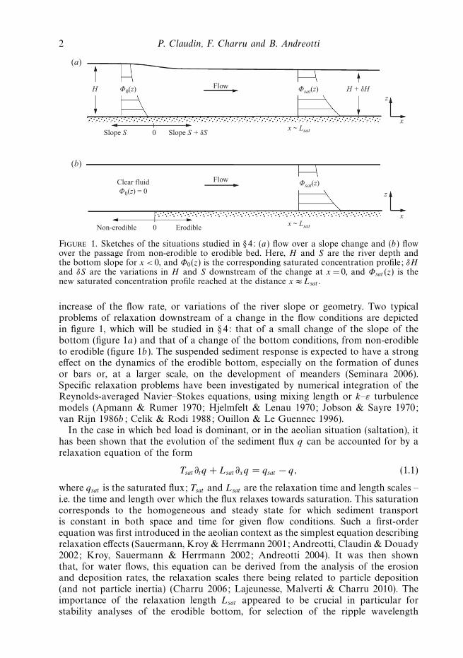
Figure 1. Sketches of the situations studied in § 4: (a) flow over a slope change and (b) flowover the passage from non-erodible to erodible bed. Here, H and S are the river depth andthe bottom slope for x < 0, and Φ0(z) is the corresponding saturated concentration profile; δHand δS are the variations in H and S downstream of the change at x =0, and Φsat (z) is thenew saturated concentration profile reached at the distance x ≈ Lsat .
increase of the flow rate, or variations of the river slope or geometry. Two typicalproblems of relaxation downstream of a change in the flow conditions are depictedin figure 1, which will be studied in § 4: that of a small change of the slope of thebottom (figure 1a) and that of a change of the bottom conditions, from non-erodibleto erodible (figure 1b). The suspended sediment response is expected to have a strongeffect on the dynamics of the erodible bottom, especially on the formation of dunesor bars or, at a larger scale, on the development of meanders (Seminara 2006).Specific relaxation problems have been investigated by numerical integration of theReynolds-averaged Navier–Stokes equations, using mixing length or k–ε turbulencemodels (Apmann & Rumer 1970; Hjelmfelt & Lenau 1970; Jobson & Sayre 1970;van Rijn 1986b; Celik & Rodi 1988; Ouillon & Le Guennec 1996).
In the case in which bed load is dominant, or in the aeolian situation (saltation), ithas been shown that the evolution of the sediment flux q can be accounted for by arelaxation equation of the form
Tsat∂tq + Lsat∂xq = qsat − q, (1.1)
where qsat is the saturated flux; Tsat and Lsat are the relaxation time and length scales –i.e. the time and length over which the flux relaxes towards saturation. This saturationcorresponds to the homogeneous and steady state for which sediment transportis constant in both space and time for given flow conditions. Such a first-orderequation was first introduced in the aeolian context as the simplest equation describingrelaxation effects (Sauermann, Kroy & Herrmann 2001; Andreotti, Claudin & Douady2002; Kroy, Sauermann & Herrmann 2002; Andreotti 2004). It was then shownthat, for water flows, this equation can be derived from the analysis of the erosionand deposition rates, the relaxation scales there being related to particle deposition(and not particle inertia) (Charru 2006; Lajeunesse, Malverti & Charru 2010). Theimportance of the relaxation length Lsat appeared to be crucial in particular forstability analyses of the erodible bottom, for selection of the ripple wavelength

Transport relaxation time and length scales in turbulent suspensions 3
(Fourriere, Claudin & Andreotti 2010). The importance of relaxation phenomena forsuspensions in turbulent flow is well known in the context of hydraulic engineering(Yalin & Finlaysen 1973; van Rijn 1986a; Celik & Rodi 1988; Ouillon & Le Guennec1996). This importance has also been recognized in the context of geomorphology;in particular, Davy & Lague (2009) proposed a deposition length of sediment as therelevant transport length. However, a derivation of a relaxation equation of the form(1.1), from firm hydrodynamic grounds, is still lacking.
In this paper, we discuss the conditions under which an equation of the form(1.1) can be derived for turbulent flows, when suspension is the dominant mode oftransport, with particular emphasis on the identification of the saturation length andtime scales. The paper is organized as follows. In the next section, we present theflow models and saturation conditions. In § 3 we perform a mode analysis of theadvection–diffusion equation for the particle concentration applied to unsaturatedcases and then identify the saturation length and time scales of the flux. The relevanceof this approach is illustrated in § 4 by treating a few examples: (i) the effect onthe sediment flux of a change in the river slope, (ii) the change from a fixed toan erodible bed and (iii) the deposition of sediments from a source near the freesurface. For the last two situations, the predictions of the model are tested againstexperimental data from the literature.
2. Flow models2.1. Logarithmic flow model
We consider the free-surface, turbulent flow of a fluid layer of thickness H over anerodible bed. For the sake of simplicity, we restrict the discussion to flows invariantin the spanwise direction, i.e. two-dimensional, with streamwise coordinate x andupward transverse coordinate z. Measurements have shown that the profile of thestreamwise velocity is close to the logarithmic law,
ux(z) =u∗
κln
(z + z0
z0
), (2.1)
where u∗ is the friction velocity; z0 is the hydrodynamical bed roughness; and κ = 0.4is the von Karman coefficient. For a steady flow in which the shear stress is balancedby the streamwise component of gravity, the shear stress increases linearly from zeroat the free surface to τb = ρu2
∗ at the bottom, so that the logarithmic velocity profile(2.1) corresponds to a parabolic eddy viscosity νt (Nezu & Rodi 1986), given by
νt
u∗H= κ
(z + z0
H
) (1 − z
H
). (2.2)
From (2.1), the depth-averaged velocity U is given by
λ ≡ U
u∗=
1
κ
[ln
(H
z0
)− 1
], (2.3)
with the typical value λ=10, corresponding to z0/H ≈ 0.01 (Raudkivi 1998).We assume that the sediment concentration φ is governed by the advection–diffusion
equation
∂φ
∂t+ ux
∂φ
∂x=
∂
∂x
(D
∂φ
∂x
)+
∂
∂z
(D
∂φ
∂z+ φVfall
), (2.4)

4 P. Claudin, F. Charru and B. Andreotti
where D is the particle eddy diffusivity and Vfall the settling velocity. Measurementshave shown that D(z) is reasonably parabolic and proportional to the eddy viscosity(2.2), with a turbulent Schmidt number
Sc =νt
D(2.5)
in the range 0.5–1 (Coleman 1970; Celik & Rodi 1988; Nielsen 1992). The settlingvelocity Vfall is taken uniform and, when needed for comparison with experiments,equal to that of a single particle in the quiescent fluid. Note that the above modellingignores inertial effects on particle motion, in particular their ejection from the coreof vortices and their clustering (Bec et al. 2007; Hunt et al. 2007). We also limit thediscussion to dilute suspensions, i.e. small volume particle concentration φ, for whichthere is no significant feedback of the particles on transport.
Solving (2.4) requires two boundary conditions, one at the free surface and one onthe sedimentary bed. At the free surface, the net vertical flux vanishes, giving
D∂φ
∂z+ φ Vfall = 0 at z = H. (2.6)
At the bottom, just above the bed-load layer where particles mainly roll and slide oneach other, the diffusive flux is equal to the erosion flux ϕ↑, i.e. the volume of particlesentrained in suspension per unit time and bed area (Parker 1978; van Rijn 1986b):
−D∂φ
∂z= ϕ↑ at z = 0. (2.7)
The erosion rate, or ‘pickup function’, is generically an increasing function ofthe basal shear stress above a threshold. Its functional form is determinedphenomenologically from experiments and depends on the nature of the bed –whether it is consolidated/cohesive or not, composed of grains or containing clay,etc. (Shields 1936; Einstein 1950; Engelund 1970; van Rijn 1984a; Briaud et al. 2001;Hanson & Simon 2001; Bonelli, Brivois & Benahmed 2007).
Two remarks have to be made here. First, the bottom condition (2.7) applies forsteady and homogeneous as well as unsteady and heterogeneous flows. In the lattercase, the erosion flux may be different from the deposition flux, so that the net fluxis non-zero, which may lead to variations of the bed topography (but not necessarily,as in the experiments to be discussed later). Possible variations in the bed topographywill be ignored here. Second, the boundary condition (2.7) corresponds to a bedallowing unlimited sediment supply. For more general situations (e.g. fixed bed),slightly different boundary conditions have been proposed (see Celik & Rodi 1988),which however requires an empirical constant or reference concentration near thebottom to be given, which varies along the channel. Finally, assuming that particleshave the same mean velocity as the fluid, ux , the flux of suspended particles, per unitlength in the spanwise direction, is given by
q =
∫ H
0
φux dz. (2.8)
The concentration equation (2.4) with the boundary condition (2.6) admits a steadyand homogeneous solution corresponding to the balance of the settling and diffusivefluxes,
Φsat (z) = Φb
(1 − z/H
1 + z/z0
)β/(1+z0/H )
, (2.9)

Transport relaxation time and length scales in turbulent suspensions 5
0.5 1.00
0.2
0.4
0.6
0.8
1.0
β = 1 0.3 0.1
Φsat/Φb
0.5 1.0
Φsat/Φb
z/H
0
0.2
0.4
0.6
0.8
1.0
α/6 = β = 1 0.3 0.1
(a) (b)
Figure 2. (a) Logarithmic flow model: normalized velocity profile (dashed line) andnormalized concentration profiles (2.9) for three values of β (solid lines). (b) Plug flowmodel: normalized concentration profiles (2.12) for the corresponding values of α = 6β .
where β , known as the Rouse number, is defined as β = (Sc Vfall )/(κ u∗), and thebottom concentration Φb = Φsat (0) is determined from the condition (2.7) as
Φb =ϕ↑(τb)
Vfall
. (2.10)
Note that (2.9) differs slightly for the classical expression of the Rouse profile (Nielsen1992) because the location at which the velocity (2.1) vanishes and the bottomboundary condition (2.7) applies has been chosen to be z = 0 instead of z = z0.Suspension typically occurs when Vfall < 0.8 u∗ (Fredsøe & Daigaard 1992), whichcorresponds to β < 4/3 with Sc =2/3. Figure 2(a) displays the velocity profile (2.1),normalized by ux(H ), and the concentration profile (2.9), normalized by Φb, for threetypical values of β .
2.2. A simplified plug flow model
In order to get analytical results, a simplified plug flow model will be used in thefollowing, which appears to provide accurate results as long as the assessment ofthe relaxation equation (1.1) is pursued. This model corresponds to the uniform flowvelocity ux(z) = U and the friction velocity u∗ = U/λ, where λ is the same constantas in the previous section. Such a plug flow model is of course a rough description,and the velocity profile actually does not switch from zero on the bed to its averagevalue on a vanishing vertical distance, leading to an infinite shear. This problem isnot present in the logarithmic model, which is more realistic from this point of view.However, as shown below, these two models do not differ much as far as the relaxationmodes are concerned, which means that what occurs very close to the bed is not veryimportant for the present purpose. Accordingly, a uniform particle diffusivity D0 willbe taken in the concentration equation (2.4) and boundary conditions (2.6) and (2.7),equal to the average of the parabolic distribution given by (2.2) and (2.5). Up to asmall correction of order z0/H , the diffusivity D0 is given by
D0
u∗H=
κ
6Sc≡ K. (2.11)
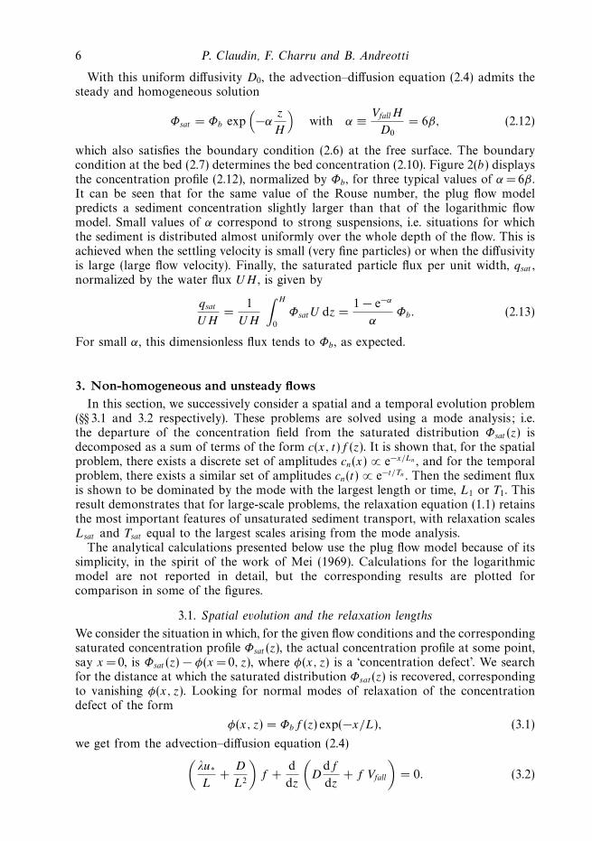
6 P. Claudin, F. Charru and B. Andreotti
With this uniform diffusivity D0, the advection–diffusion equation (2.4) admits thesteady and homogeneous solution
Φsat = Φb exp(
−αz
H
)with α ≡ VfallH
D0
= 6β, (2.12)
which also satisfies the boundary condition (2.6) at the free surface. The boundarycondition at the bed (2.7) determines the bed concentration (2.10). Figure 2(b) displaysthe concentration profile (2.12), normalized by Φb, for three typical values of α = 6β .It can be seen that for the same value of the Rouse number, the plug flow modelpredicts a sediment concentration slightly larger than that of the logarithmic flowmodel. Small values of α correspond to strong suspensions, i.e. situations for whichthe sediment is distributed almost uniformly over the whole depth of the flow. This isachieved when the settling velocity is small (very fine particles) or when the diffusivityis large (large flow velocity). Finally, the saturated particle flux per unit width, qsat ,normalized by the water flux UH , is given by
qsat
UH=
1
UH
∫ H
0
ΦsatU dz =1 − e−α
αΦb. (2.13)
For small α, this dimensionless flux tends to Φb, as expected.
3. Non-homogeneous and unsteady flowsIn this section, we successively consider a spatial and a temporal evolution problem
(§§ 3.1 and 3.2 respectively). These problems are solved using a mode analysis; i.e.the departure of the concentration field from the saturated distribution Φsat (z) isdecomposed as a sum of terms of the form c(x, t)f (z). It is shown that, for the spatialproblem, there exists a discrete set of amplitudes cn(x) ∝ e−x/Ln , and for the temporalproblem, there exists a similar set of amplitudes cn(t) ∝ e−t/Tn . Then the sediment fluxis shown to be dominated by the mode with the largest length or time, L1 or T1. Thisresult demonstrates that for large-scale problems, the relaxation equation (1.1) retainsthe most important features of unsaturated sediment transport, with relaxation scalesLsat and Tsat equal to the largest scales arising from the mode analysis.
The analytical calculations presented below use the plug flow model because of itssimplicity, in the spirit of the work of Mei (1969). Calculations for the logarithmicmodel are not reported in detail, but the corresponding results are plotted forcomparison in some of the figures.
3.1. Spatial evolution and the relaxation lengths
We consider the situation in which, for the given flow conditions and the correspondingsaturated concentration profile Φsat (z), the actual concentration profile at some point,say x = 0, is Φsat (z) − φ(x = 0, z), where φ(x, z) is a ‘concentration defect’. We searchfor the distance at which the saturated distribution Φsat (z) is recovered, correspondingto vanishing φ(x, z). Looking for normal modes of relaxation of the concentrationdefect of the form
φ(x, z) = Φbf (z) exp(−x/L), (3.1)
we get from the advection–diffusion equation (2.4)(λu∗
L+
D
L2
)f +
d
dz
(D
df
dz+ f Vfall
)= 0. (3.2)

Transport relaxation time and length scales in turbulent suspensions 7
0.5 1.0 1.5 2.00
1
2
3
4
5
6
7
n = 3
2
1
α0.5 1.0 1.5 2.0
α
Kin
0
0.2
0.4
0.6
0.8
1.0
n = 1
2
3
Ln/
Ld
(a) (b)
Figure 3. (a) Variation with α of the three smallest roots of (3.6). (b) Corresponding relaxationnormalized lengths Ln/Ld for λ/K = 50: solid lines, plug flow; dashed lines, logarithmic flow.
At the free surface, the zero flux condition (2.6) gives
Ddf
dz+ f Vfall = 0 at z = H. (3.3)
On the bed the friction velocity u∗ is assumed to be uniform. The erosion flux ϕ↑,which depends only on u∗, is uniform too. Hence, the disturbance of ϕ↑ is zero, sothat, from (2.7),
df
dz= 0 at z = 0. (3.4)
The above differential problem is solved numerically for parabolic D (logarithmicflow model) and analytically for uniform D = D0 (plug flow model). For uniform D0,(3.2) has solutions of the form f (z) ∝ exp(Kz/H ), where K has to satisfy a q uadraticequation with roots K+ and K− given by
K± = −α
2± iKi with Ki =
√λ
KH
L+
H 2
L2− α2
4. (3.5)
Then the boundary conditions (3.3) and (3.4) select a discrete set of relaxation lengthsL, satisfying
tan Ki =
(Ki
α− α
4Ki
)−1
. (3.6)
This equation has an infinite number of real positive solutions Kin, n � 1. Figure 3(a)shows the variation with α of the three smallest ones (n= 1, 2, 3). For small α, thesesolutions behave as Ki1 ∼
√α and Kin ∼ (n − 1)π for n � 2.
The corresponding relaxation lengths Ln are found from (3.5):
H
Ln
=1
2
⎛⎝− λ
K ±
√(λ
K
)2
+ α2 + 4K2in
⎞⎠ , n � 1. (3.7)
They are displayed for n= 1, 2, 3 in figure 3(b) as a function of α (solid lines),normalized with the characteristic deposition length
Ld ≡ U
Vfall
H. (3.8)

8 P. Claudin, F. Charru and B. Andreotti
0–1.0 –0.5 0 0.5 1.0
0.2
0.4
0.6
0.8
1.0
2 3 n = 1
z/H
fn
2 3 n = 1
(a)
0–1.0 –0.5 0 0.5 1.0
0.2
0.4
0.6
0.8
1.0
fn
(b)
Figure 4. Profile of the three first eigenfunctions fn(z), for α = (a) 0.1 and (b) 1: solid lines,plug flow; dashed lines, logarithmic flow.
It can be seen that L1 is much larger than the higher-order relaxation lengths –typically by one order of magnitude. Remarkably, in the limit of small α (largeflow velocity or small settling velocity), the largest length L1 tends to Ld , whereashigher-order lengths remain of the order of the flow depth H :
L1 ∼ Ld, Ln ∼ λ/K(n − 1)2π2
H for n � 2. (3.9)
Figure 3(b) also displays the normalized relaxation lengths obtained from thelogarithmic flow model (dashed lines), from numerical integration of (3.2) withparabolic D. It can be seen that these lengths are close to those from the plugflow model, especially for the largest length L1. Note that Ln/Ld is weakly sensitiveto the value of λ/K: doubling this ratio does not bring any visible change, at leastfor α � 2.
The eigenfunctions fn(z) are given by
fn(z) =
[cos
(Kin
z
H
)+
α
2Kin
sin(Kin
z
H
)]exp
(−α
2
z
H
), n � 1, (3.10)
with the normalization condition fn(0) = 1. These eigenfunctions are displayed infigure 4 for n=1, 2, 3 (solid lines), for α =0.1 (figure 4a) and α = 1 (figure 4b).It can be seen that f1(z) decreases slightly and monotonically from the bottom tothe top, whereas higher-order eigenfunctions oscillate, more and more strongly withincreasing n. Figure 4 also displays the eigenfunctions from the logarithmic flowmodel (dashed lines). It can be seen that for the mode associated with the largestlength L1 (n= 1), eigenfunctions of both models remain very close to each other andthat differences become larger as n increases.
Let us turn to the sediment flux. The contribution of the nth eigenmode to thesediment flux Qn, normalized with the characteristic sediment flux UHΦb and theexponential x-dependence, is
1
exp(−x/Ln)
1
ΦbUHQn =
1
H
∫ H
0
fn(z) dz. (3.11)
Table 1(a) displays the contribution of each of the first three modes to the sedimentflux, i.e. the right-hand side of the above equation. It can be seen that the contribution
Transport relaxation time and length scales in turbulent suspensions 9
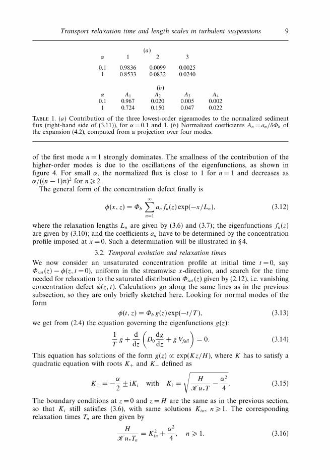
(a)α 1 2 3
0.1 0.9836 0.0099 0.00251 0.8533 0.0832 0.0240
(b)α A1 A2 A3 A4
0.1 0.967 0.020 0.005 0.0021 0.724 0.150 0.047 0.022
Table 1. (a) Contribution of the three lowest-order eigenmodes to the normalized sedimentflux (right-hand side of (3.11)), for α = 0.1 and 1. (b) Normalized coefficients An = an/δΦb ofthe expansion (4.2), computed from a projection over four modes.
of the first mode n= 1 strongly dominates. The smallness of the contribution of thehigher-order modes is due to the oscillations of the eigenfunctions, as shown infigure 4. For small α, the normalized flux is close to 1 for n= 1 and decreases asα/((n − 1)π)2 for n � 2.
The general form of the concentration defect finally is
φ(x, z) = Φb
∞∑n=1
anfn(z) exp(−x/Ln), (3.12)
where the relaxation lengths Ln are given by (3.6) and (3.7); the eigenfunctions fn(z)are given by (3.10); and the coefficients an have to be determined by the concentrationprofile imposed at x = 0. Such a determination will be illustrated in § 4.
3.2. Temporal evolution and relaxation times
We now consider an unsaturated concentration profile at initial time t = 0, sayΦsat (z) − φ(z, t = 0), uniform in the streamwise x-direction, and search for the timeneeded for relaxation to the saturated distribution Φsat (z) given by (2.12), i.e. vanishingconcentration defect φ(z, t). Calculations go along the same lines as in the previoussubsection, so they are only briefly sketched here. Looking for normal modes of theform
φ(t, z) = Φb g(z) exp(−t/T ), (3.13)
we get from (2.4) the equation governing the eigenfunctions g(z):
1
Tg +
d
dz
(D0
dg
dz+ g Vfall
)= 0. (3.14)
This equation has solutions of the form g(z) ∝ exp(Kz/H ), where K has to satisfy aquadratic equation with roots K+ and K− defined as
K± = −α
2± iKi with Ki =
√H
Ku∗T− α2
4. (3.15)
The boundary conditions at z =0 and z = H are the same as in the previous section,so that Ki still satisfies (3.6), with same solutions Kin, n � 1. The correspondingrelaxation times Tn are then given by
H
Ku∗Tn
= K2in +
α2
4, n � 1. (3.16)
10 P. Claudin, F. Charru and B. Andreotti
Introducing the characteristic deposition time
Td ≡ H
Vfall
=Ld
U, (3.17)
the relaxation times are, in the limit of small α,
T1 ∼ Td, Tn ∼ αTd
(n − 1)2π2∼ Ln
Ufor n � 2. (3.18)
As for the spatial problem, the sediment dynamics is dominated by the largest timeT1, equal to the deposition time Td for strong suspensions.
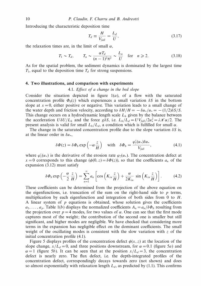
4. Two illustrations, and comparison with experiments4.1. Effect of a change in the bed slope
Consider the situation depicted in figure 1(a), of a flow with the saturatedconcentration profile Φ0(z) which experiences a small variation δS in the bottomslope at x = 0, either positive or negative. This variation leads to a small change ofthe water depth and friction velocity, according to δH/H = − δu∗/u∗ = − (1/2)δS/S.This change occurs on a hydrodynamic length scale Lh given by the balance betweenthe acceleration UδU/Lh and the force gδS, i.e. Lh/Ld = UVfall/2u2
∗ = λKα/2. Thepresent analysis is valid for small Lh/Ld , a condition which is fulfilled for small α.
The change in the saturated concentration profile due to the slope variation δS is,at the linear order in δu∗,
δΦ(z) = δΦb exp(
−αz
H
)with δΦb =
ϕ′↑(u∗)δu∗
Vfall
, (4.1)
where ϕ′↑(u∗) is the derivative of the erosion rate ϕ↑(u∗). The concentration defect at
x = 0 corresponds to this change (φ(0, z) = δΦ(z)), so that the coefficients an of theexpansion (3.12) must satisfy
δΦb exp(
−α
2
z
H
)=
∞∑n=1
an
[cos
(Kin
z
H
)+
α
2Kin
sin(Kin
z
H
)]. (4.2)
These coefficients can be determined from the projection of the above equation onthe eigenfunctions, i.e. truncation of the sum on the right-hand side to p terms,multiplication by each eigenfunction and integration of both sides from 0 to H .A linear system of p equations is obtained, whose solution gives the coefficientsa1, . . . , ap . Table 1(b) displays the normalized coefficients An = an/δΦb resulting fromthe projection over p = 4 modes, for two values of α. One can see that the first modecaptures most of the weight; the contribution of the second one is smaller but stillsignificant, and higher modes are negligible. We have checked that considering moreterms in the expansion has negligible effect on the dominant coefficients. The smallweight of the oscillating modes is consistent with the slow variation with z of theinitial concentration profile (4.1).
Figure 5 displays profiles of the concentration defect φ(x, z) at the location of theslope change, x/Ld = 0, and three positions downstream, for α =0.1 (figure 5a) andα = 1 (figure 5b). It can be seen that at the position x/Ld = 3, the concentrationdefect is nearly zero. The flux defect, i.e. the depth-integrated profiles of theconcentration defect, correspondingly decays towards zero (not shown) and doesso almost exponentially with relaxation length Ld , as predicted by (1.1). This confirms
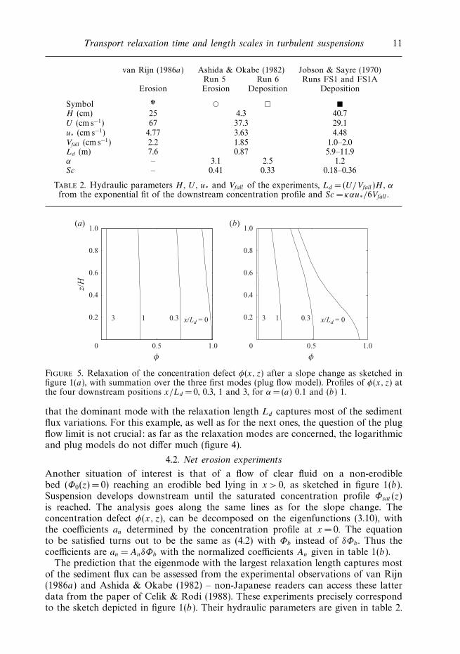
Transport relaxation time and length scales in turbulent suspensions 11
van Rijn (1986a) Ashida & Okabe (1982) Jobson & Sayre (1970)Run 5 Run 6 Runs FS1 and FS1A
Erosion Erosion Deposition Deposition
Symbol ∗ � � �
H (cm) 25 4.3 40.7U (cm s−1) 67 37.3 29.1u∗ (cm s−1) 4.77 3.63 4.48Vfall (cm s−1) 2.2 1.85 1.0–2.0Ld (m) 7.6 0.87 5.9–11.9α – 3.1 2.5 1.2Sc – 0.41 0.33 0.18–0.36
Table 2. Hydraulic parameters H , U , u∗ and Vfall of the experiments, Ld = (U/Vfall )H , αfrom the exponential fit of the downstream concentration profile and Sc = καu∗/6Vfall .
0.5 1.00
0.2
0.4
0.6
0.8
1.0
3 1 0.3 x/Ld = 0
φ
3 1 x/Ld = 0
z/H
(a)
0.5 1.00
0.2
0.4
0.6
0.8
1.0
φ
(b)
0.3
Figure 5. Relaxation of the concentration defect φ(x, z) after a slope change as sketched infigure 1(a), with summation over the three first modes (plug flow model). Profiles of φ(x, z) atthe four downstream positions x/Ld = 0, 0.3, 1 and 3, for α = (a) 0.1 and (b) 1.
that the dominant mode with the relaxation length Ld captures most of the sedimentflux variations. For this example, as well as for the next ones, the question of the plugflow limit is not crucial: as far as the relaxation modes are concerned, the logarithmicand plug models do not differ much (figure 4).
4.2. Net erosion experiments
Another situation of interest is that of a flow of clear fluid on a non-erodiblebed (Φ0(z) = 0) reaching an erodible bed lying in x > 0, as sketched in figure 1(b).Suspension develops downstream until the saturated concentration profile Φsat (z)is reached. The analysis goes along the same lines as for the slope change. Theconcentration defect φ(x, z), can be decomposed on the eigenfunctions (3.10), withthe coefficients an determined by the concentration profile at x = 0. The equationto be satisfied turns out to be the same as (4.2) with Φb instead of δΦb. Thus thecoefficients are an = AnδΦb with the normalized coefficients An given in table 1(b).
The prediction that the eigenmode with the largest relaxation length captures mostof the sediment flux can be assessed from the experimental observations of van Rijn(1986a) and Ashida & Okabe (1982) – non-Japanese readers can access these latterdata from the paper of Celik & Rodi (1988). These experiments precisely correspondto the sketch depicted in figure 1(b). Their hydraulic parameters are given in table 2.
12 P. Claudin, F. Charru and B. Andreotti
1 2 3 40
1
Φsat /Φref
2 4 6 8
x/Ld
q/q s
at
z/H
(a)
0
1(b)
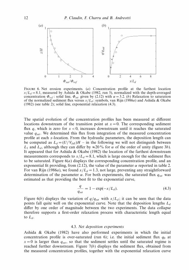
Figure 6. Net erosion experiments. (a) Concentration profile at the farthest locationx/Ld = 8.1, measured by Ashida & Okabe (1982, run 5), normalized with the depth-averagedconcentration Φref : solid line, Φsat given by (2.12) with α = 3.2. (b) Relaxation to saturationof the normalized sediment flux versus x/Ld : symbols, van Rijn (1986a) and Ashida & Okabe(1982) (see table 2); solid line, exponential relaxation (4.3).
The spatial evolution of the concentration profiles has been measured at differentlocations downstream of the transition point at x =0. The corresponding sedimentflux q , which is zero for x < 0, increases downstream until it reaches the saturatedvalue qsat . We determined this flux from integration of the measured concentrationprofile at each x-location. From the hydraulic parameters, the deposition length canbe computed as Ld =(U/Vfall )H – in the following we will not distinguish betweenL1 and Ld , although they can differ by ≈20 % for α of the order of unity (figure 3b).It appeared that for Ashida & Okabe (1982) the location of the farthest downstreammeasurements corresponds to x/Ld = 8.1, which is large enough for the sediment fluxto be saturated. Figure 6(a) displays the corresponding concentration profile, and anexponential fit providing, from (2.12), the value of the parameter α reported in table 2.For van Rijn (1986a), we found x/Ld = 1.3, not large, preventing any straightforwarddetermination of the parameter α. For both experiments, the saturated flux qsat wasestimated as that providing the best fit to the exponential curve,
q
qsat
= 1 − exp(−x/Ld). (4.3)
Figure 6(b) displays the variation of q/qsat with x/Ld; it can be seen that the datapoints fall quite well on the exponential curve. Note that the deposition lengths Ld
differ by one order of magnitude between the two experiments. The data collapsetherefore supports a first-order relaxation process with characteristic length equalto Ld .
4.3. Net deposition experiments
Ashida & Okabe (1982) have also performed experiments in which the initialconcentration profile is over-saturated (run 6); i.e. the initial sediment flux q0 atx = 0 is larger than qsat , so that the sediment settles until the saturated regime isreached further downstream. Figure 7(b) displays the sediment flux, obtained fromthe measured concentration profiles, together with the exponential relaxation curve
Transport relaxation time and length scales in turbulent suspensions 13
0.5 1.0 1.5 2.00
0.2
0.4
0.6
0.8
1.0
2 4 6 80
1
2
3
4
Φ0/Φref
z/H
(a)
x/Ld
q/q s
at
(b)
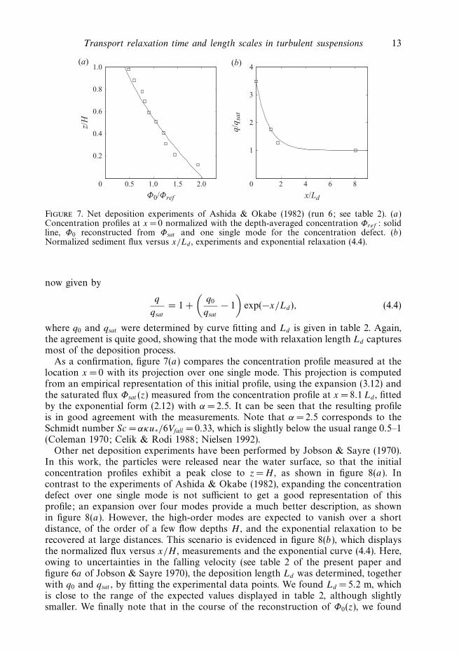
Figure 7. Net deposition experiments of Ashida & Okabe (1982) (run 6; see table 2). (a)Concentration profiles at x = 0 normalized with the depth-averaged concentration Φref : solidline, Φ0 reconstructed from Φsat and one single mode for the concentration defect. (b)Normalized sediment flux versus x/Ld , experiments and exponential relaxation (4.4).
now given by
q
qsat
= 1 +
(q0
qsat
− 1
)exp(−x/Ld), (4.4)
where q0 and qsat were determined by curve fitting and Ld is given in table 2. Again,the agreement is quite good, showing that the mode with relaxation length Ld capturesmost of the deposition process.
As a confirmation, figure 7(a) compares the concentration profile measured at thelocation x = 0 with its projection over one single mode. This projection is computedfrom an empirical representation of this initial profile, using the expansion (3.12) andthe saturated flux Φsat (z) measured from the concentration profile at x = 8.1 Ld , fittedby the exponential form (2.12) with α = 2.5. It can be seen that the resulting profileis in good agreement with the measurements. Note that α = 2.5 corresponds to theSchmidt number Sc =ακu∗/6Vfall = 0.33, which is slightly below the usual range 0.5–1(Coleman 1970; Celik & Rodi 1988; Nielsen 1992).
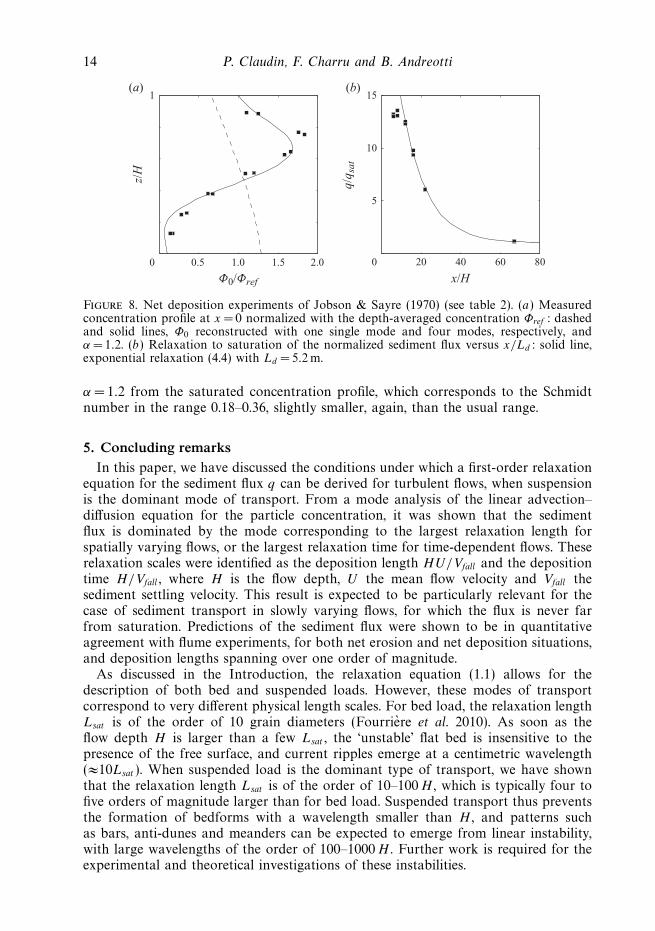
Other net deposition experiments have been performed by Jobson & Sayre (1970).In this work, the particles were released near the water surface, so that the initialconcentration profiles exhibit a peak close to z = H , as shown in figure 8(a). Incontrast to the experiments of Ashida & Okabe (1982), expanding the concentrationdefect over one single mode is not sufficient to get a good representation of thisprofile; an expansion over four modes provide a much better description, as shownin figure 8(a). However, the high-order modes are expected to vanish over a shortdistance, of the order of a few flow depths H , and the exponential relaxation to berecovered at large distances. This scenario is evidenced in figure 8(b), which displaysthe normalized flux versus x/H , measurements and the exponential curve (4.4). Here,owing to uncertainties in the falling velocity (see table 2 of the present paper andfigure 6a of Jobson & Sayre 1970), the deposition length Ld was determined, togetherwith q0 and qsat , by fitting the experimental data points. We found Ld = 5.2 m, whichis close to the range of the expected values displayed in table 2, although slightlysmaller. We finally note that in the course of the reconstruction of Φ0(z), we found
14 P. Claudin, F. Charru and B. Andreotti
0.5 1.0 1.5 2.00
1
20 40 60 800
5
10
15
x/HΦ0/Φref
z/H
(a)
q/q s
at
(b)
Figure 8. Net deposition experiments of Jobson & Sayre (1970) (see table 2). (a) Measuredconcentration profile at x = 0 normalized with the depth-averaged concentration Φref : dashedand solid lines, Φ0 reconstructed with one single mode and four modes, respectively, andα = 1.2. (b) Relaxation to saturation of the normalized sediment flux versus x/Ld : solid line,exponential relaxation (4.4) with Ld = 5.2 m.
α = 1.2 from the saturated concentration profile, which corresponds to the Schmidtnumber in the range 0.18–0.36, slightly smaller, again, than the usual range.
5. Concluding remarksIn this paper, we have discussed the conditions under which a first-order relaxation
equation for the sediment flux q can be derived for turbulent flows, when suspensionis the dominant mode of transport. From a mode analysis of the linear advection–diffusion equation for the particle concentration, it was shown that the sedimentflux is dominated by the mode corresponding to the largest relaxation length forspatially varying flows, or the largest relaxation time for time-dependent flows. Theserelaxation scales were identified as the deposition length HU/Vfall and the depositiontime H/Vfall , where H is the flow depth, U the mean flow velocity and Vfall thesediment settling velocity. This result is expected to be particularly relevant for thecase of sediment transport in slowly varying flows, for which the flux is never farfrom saturation. Predictions of the sediment flux were shown to be in quantitativeagreement with flume experiments, for both net erosion and net deposition situations,and deposition lengths spanning over one order of magnitude.
As discussed in the Introduction, the relaxation equation (1.1) allows for thedescription of both bed and suspended loads. However, these modes of transportcorrespond to very different physical length scales. For bed load, the relaxation lengthLsat is of the order of 10 grain diameters (Fourriere et al. 2010). As soon as theflow depth H is larger than a few Lsat , the ‘unstable’ flat bed is insensitive to thepresence of the free surface, and current ripples emerge at a centimetric wavelength(≈10Lsat ). When suspended load is the dominant type of transport, we have shownthat the relaxation length Lsat is of the order of 10–100 H , which is typically four tofive orders of magnitude larger than for bed load. Suspended transport thus preventsthe formation of bedforms with a wavelength smaller than H , and patterns suchas bars, anti-dunes and meanders can be expected to emerge from linear instability,with large wavelengths of the order of 100–1000 H . Further work is required for theexperimental and theoretical investigations of these instabilities.
Transport relaxation time and length scales in turbulent suspensions 15
This work has benefited from the financial support of the Agence Nationale de laRecherche, grant Zephyr (no. ERCS07 18) and the GdR MePhy of the CNRS (no.3166).
REFERENCES
Andreotti, B. 2004 A two species model of aeolian sand transport. J. Fluid Mech. 510, 47–50.
Andreotti, B., Claudin, P. & Douady, S. 2002 Selection of dune shapes and velocities. Eur. J.Phys. B 28, 341.
Apmann, R. P. & Rumer, R. R. 1970 Diffusion of sediment in developing flow. J. Hydraul. Div.ASCE 96, 109–123.
Ashida, K. & Okabe, T. 1982 On the calculation method of the concentration of suspended sedimentunder non-equilibrium condition (in Japanese). In Proceedings of the 26th Conference onHydraulics, pp. 153–158. JSCE.
Bec, J., Biferale, L., Cencini, M., Lanotte, A., Musacchio, S. & Toschi, F. 2007 Heavy particleconcentration in turbulence at dissipative and inertial scales. Phys. Rev. Lett. 98, 084502.
Bonelli, S., Brivois, O. & Benahmed, N. 2007 Modelisation du renard hydraulique et interpretationde l’essai d’erosion de trou. Rev. Fr. Geotech. 118, 13–22.
Briaud, J. L., Ting, F. C. K., Chen, H. C., Cao, Y., Han, S. W. & Kwak, K. W. 2001 Erosionfunction apparatus for scour rate predictions. J. Geotech. Geoenviron. Engng 127, 105–113.
Celik, I. & Rodi, W. 1988 Modeling suspended sediment transport in nonequilibrium situations.J. Hydraul. Engng 114, 1157–1191.
Charru, F. 2006 Selection of the ripple length on a granular bed sheared by a liquid flow. Phys.Fluids 18, 121508.
Coleman, N. L. 1970 Flume studies of the sediment transfer coefficient. Water Resour. Res. 6,801–809.
Davy, P. & Lague, D. 2009 Fluvial erosion/transport equation of landscape evolution modelsrevisited. J. Geophys. Res. 114, F03007.
Einstein, H. A. 1950 The bedload function for sediment transportation in open channel flow. Tech.Bull. 1026, pp. 1–71. US Department of Agriculture.
Engelund, F. 1970 Instability of erodible beds. J. Fluid Mech. 42, 225–244.
Fourriere, A., Claudin, P. & Andreotti, B. 2010 Bedforms in a turbulent stream: formation ofripples by primary linear instability and of dunes by non-linear pattern coarsening. J. FluidMech. 649, 287–328.
Fredsøe, J. & Deigaard, R. 1992 Mechanics of Coastal Sediment Transport. World Scientific.
Hanson, G. J. & Simon, A. 2001 Erodibility of cohesive streambeds in the loess area of themidwestern USA. Hydraul. Process. 15, 23–38.
Hjelmfelt, A. T. & Lenau, C. W. 1970 Nonequilibrium transport of suspended sediment. J. Hydraul.Div. ASCE 96, 1567–1586.
Hunt, J. C. R., Delfos, R., Eames, I. & Perkins, R. 2007 Vortices, complex flows and inertialparticles. Flow Turbul. Combust. 79, 207–234.
Jobson, A. E. & Sayre, W. W. 1970 Vertical transfer in open channel flow. J. Hydraul. Div. ASCE96, 703–724.
Kroy, K., Sauermann, G. & Herrmann, H. J. 2002 Minimal model for aeolian sand dunes. Phys.Rev. E 66, 031302.
Lajeunesse, E., Malverti, L. & Charru, F. 2010 Bedload transport in turbulent flow at the grainscale: experiments and modeling. J. Geophys. Res. 115, F04001.
Mei, C. C. 1969 Nonuniform diffusion of suspended sediment. J. Hydraul. Div. ASCE 95, 581–584.
Nezu, I. 2005 Open-channel flow turbulence and its research prospect in the 21st century. J. Hydraul.Engng 131, 229–246.
Nezu, I. & Rodi, W. 1986, Open-channel flow measurements with a laser doppler anemometer.J. Hydraul. Engng. 112, 335–355.
Nielsen, P. 1992 Coastal Bottom Boundary Layers and Sediment Transport. World Scientific.
Ouillon, S. & Le Guennec, B. 1996 Modelling non-cohesive suspended sediment transport in 2Dvertical free surface flows. J. Hydraul. Res. 34, 219–236.

16 P. Claudin, F. Charru and B. Andreotti
Parker, G. 1978 Self-formed straight rivers with equilibrium banks and mobile bed. Part 1. Thesand–silt river. J. Fluid Mech. 89, 109–125.
Raudkivi, A. J. 1998 Loose Boundary Hydraulics. A. A. Balkema.
van Rijn, L. C. 1984a Sediment pick-up functions. J. Hydraul. Engng 110, 1494–1502.
van Rijn, L. C. 1984b Sediment transport. Part II. Suspended load transport. J. Hydraul. Engng110, 1613–1641.
van Rijn, L. C. 1986a Application of sediment pickup function. J. Hydraul. Engng 112, 867–874.
van Rijn, L. C. 1986b Mathematical modeling of suspended sediment in nonuniform flows.J. Hydraul. Engng 112, 433–455.
Rouse, H. 1936 Modern conceptions of the mechanics of fluid turbulence. Trans. ASCE 102,463–543.
Sauermann, G., Kroy, K. & Herrmann, H. J. 2001 A phenomenological dynamic saltation modelfor dune formation. Phys. Rev. E 64, 031305.
Seminara, G. 2006 Meanders. J. Fluid Mech. 554, 271–297.
Shields, A. 1936 Application of similarity principles and turbulence research to bed-load movement.Mitteilungen der Preussischen Versuchsanstalt fur Wasserbau und Schiffbau (ed. W.D. Ott & C.von Uchelen), vol. 26, pp. 5–24. Soil Conservation Service, California Institute of Technology.
Vanoni, V. A. 1946 Transportation of suspended sediment by water. Trans. ASCE 111, 67–133.
Yalin, K. S. & Finlaysen, G. D. 1973 On the development of the distribution of suspended load.In Proceedings of the 15th IAHR Congress, Istanbul (ed. S. Okyay), pp. 287–294.