TRANSPORT OPTIMALCedric-slides.pdf · TRANSPORT OPTIMAL Monge rencontre Riemann ENSTA, 28 octobre...
56
TRANSPORT OPTIMAL Monge rencontre Riemann ENSTA, 28 octobre 2010 C´ edric Villani Universit´ e de Lyon & Institut Henri Poincar´ e
Transcript of TRANSPORT OPTIMALCedric-slides.pdf · TRANSPORT OPTIMAL Monge rencontre Riemann ENSTA, 28 octobre...
TRANSPORT OPTIMAL
Monge rencontre Riemann
ENSTA, 28 octobre 2010
Cedric Villani
Universite de Lyon& Institut Henri Poincare

Mesure image, ou changement de variables
µ(dx), ν(dy) deux mesures (de probabilite)
y = T (x)
Def: T#µ = ν si ∀B, µ[T−1(B)] = ν[B]

Mesure image, ou changement de variables
µ(dx), ν(dy) deux mesures (de probabilite)
y = T (x)
Def: T#µ = ν si ∀B, µ[T−1(B)] = ν[B]
Equivalent: ∀ϕ,
∫
ϕ T dµ =
∫
ϕ d(T#µ)

Mesure image, ou changement de variables
µ(dx), ν(dy) deux mesures (de probabilite)
y = T (x)
Def: T#µ = ν si ∀B, µ[T−1(B)] = ν[B]
Equivalent: ∀ϕ,
∫
ϕ T dµ =
∫
ϕ d(T#µ)
Formulation probabiliste
loi (U) = µ, loi (V ) = ν, V = T (U)

Mesure image, ou changement de variables
µ(dx), ν(dy) deux mesures (de probabilite)
y = T (x)
Def: T#µ = ν si ∀B, µ[T−1(B)] = ν[B]
Equivalent: ∀ϕ,
∫
ϕ T dµ =
∫
ϕ d(T#µ)
Formulation probabiliste
loi (U) = µ, loi (V ) = ν, V = T (U)
Formulation analytique
Dans Rn, T#(f(x) dx) = g(y) dy, T injective ⇒
f(x) = g(T (x)) | det(dT )(x)|

PROBLEME DE MONGE–KANTOROVICH

µ(dx), ν(dy) deux mesures de probabilite
c(x, y) fonction de cout
(MK) infT#µ=ν
∫
c(x, T (x)) dµ(x)
µ
deblaisremblais
x
T
νy
transporter des materiaux au moindre cout,
distributions de masse initiale et finale fixees

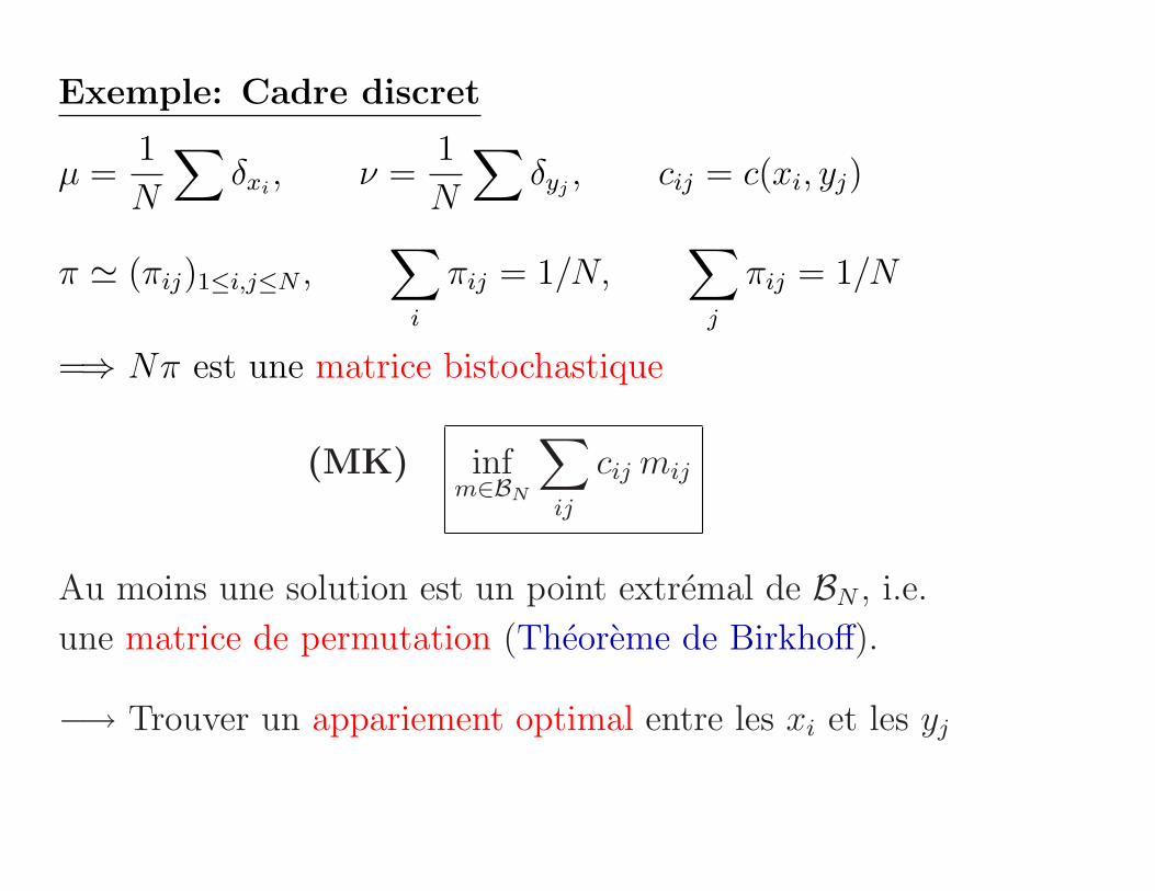
Exemple: Cadre discret
µ =1
N
∑
δxi, ν =
1
N
∑
δyj, cij = c(xi, yj)
π ≃ (πij)1≤i,j≤N ,∑
i
πij = 1/N,∑
j
πij = 1/N
=⇒ Nπ est une matrice bistochastique

Exemple: Cadre discret
µ =1
N
∑
δxi, ν =
1
N
∑
δyj, cij = c(xi, yj)
π ≃ (πij)1≤i,j≤N ,∑
i
πij = 1/N,∑
j
πij = 1/N
=⇒ Nπ est une matrice bistochastique
(MK) infm∈BN
∑
ij
cij mij
Exemple: Cadre discret
µ =1
N
∑
δxi, ν =
1
N
∑
δyj, cij = c(xi, yj)
π ≃ (πij)1≤i,j≤N ,∑
i
πij = 1/N,∑
j
πij = 1/N
=⇒ Nπ est une matrice bistochastique
(MK) infm∈BN
∑
ij
cij mij
Au moins une solution est un point extremal de BN , i.e.
une matrice de permutation (Theoreme de Birkhoff).
−→ Trouver un appariement optimal entre les xi et les yj

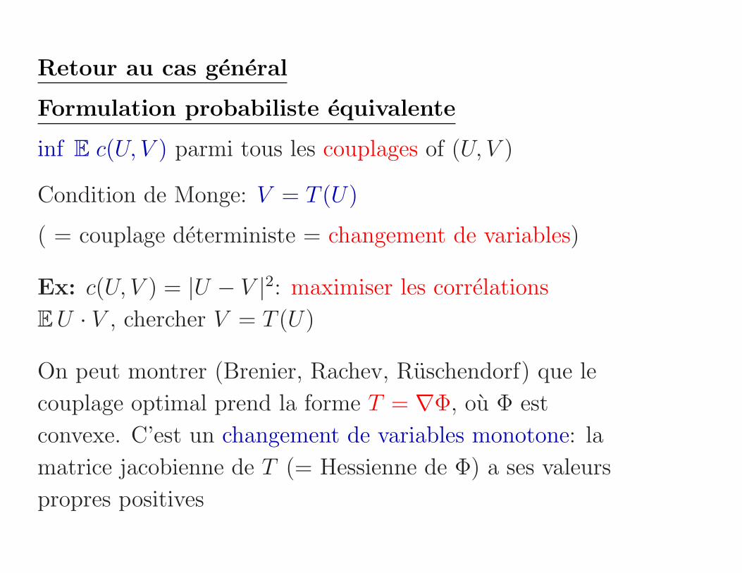
Retour au cas general
Formulation probabiliste equivalente
inf E c(U, V ) parmi tous les couplages of (U, V )
Condition de Monge: V = T (U)
( = couplage deterministe = changement de variables)
Ex: c(U, V ) = |U − V |2: maximiser les correlations
E U · V , chercher V = T (U)
Retour au cas general
Formulation probabiliste equivalente
inf E c(U, V ) parmi tous les couplages of (U, V )
Condition de Monge: V = T (U)
( = couplage deterministe = changement de variables)
Ex: c(U, V ) = |U − V |2: maximiser les correlations
E U · V , chercher V = T (U)
On peut montrer (Brenier, Rachev, Ruschendorf) que le
couplage optimal prend la forme T = ∇Φ, ou Φ est
convexe. C’est un changement de variables monotone: la
matrice jacobienne de T (= Hessienne de Φ) a ses valeurs
propres positives

Les changements de variables monotones sont puissants

Isoperimetrie euclidienne
Le volume etant fixe, la sphere minimise la surface
Ω
B
|Ω| = Ln[Ω] = volume n-dim de Ω
|∂Ω| = Hn−1[∂Ω] = volume (n − 1)-dim de ∂Ω

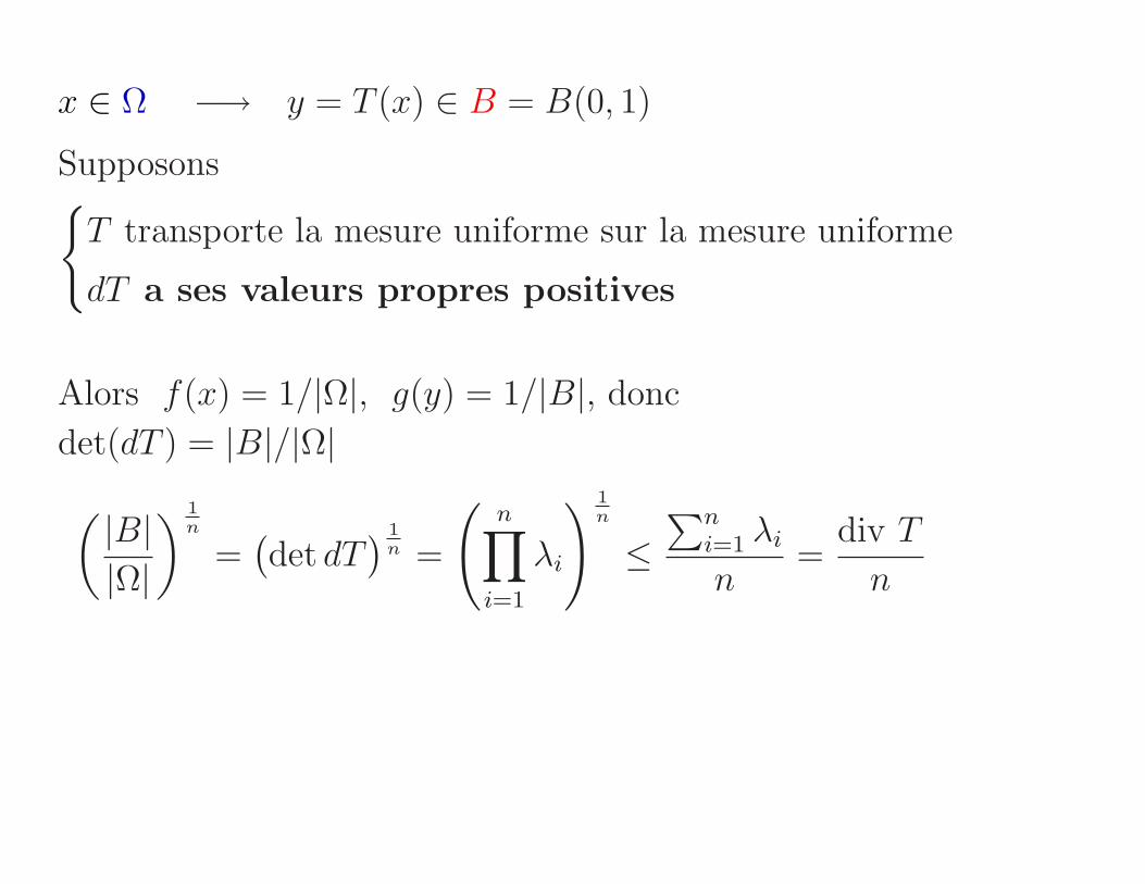
x ∈ Ω −→ y = T (x) ∈ B = B(0, 1)
Supposons
T transporte la mesure uniforme sur la mesure uniforme
dT a ses valeurs propres positives

x ∈ Ω −→ y = T (x) ∈ B = B(0, 1)
Supposons
T transporte la mesure uniforme sur la mesure uniforme
dT a ses valeurs propres positives
Alors f(x) = 1/|Ω|, g(y) = 1/|B|, donc
det(dT ) = |B|/|Ω|
x ∈ Ω −→ y = T (x) ∈ B = B(0, 1)
Supposons
T transporte la mesure uniforme sur la mesure uniforme
dT a ses valeurs propres positives
Alors f(x) = 1/|Ω|, g(y) = 1/|B|, donc
det(dT ) = |B|/|Ω|( |B||Ω|
)1n
=(
det dT)
1n =
(
n∏
i=1
λi
)1n
≤∑n
i=1 λi
n=
div T
n

x ∈ Ω −→ y = T (x) ∈ B = B(0, 1)
Supposons
T transporte la mesure uniforme sur la mesure uniforme
dT a ses valeurs propres positives
Alors f(x) = 1/|Ω|, g(y) = 1/|B|, donc
det(dT ) = |B|/|Ω|( |B||Ω|
)1n
=(
det dT)
1n =
(
n∏
i=1
λi
)1n
≤∑n
i=1 λi
n=
div T
n
|Ω| ×( |B||Ω|
)1n
≤∫
Ω
div T
n=
1
n
∫
∂Ω
T ·ν ≤ 1
n
∫
∂Ω
‖T‖ =|∂Ω|n

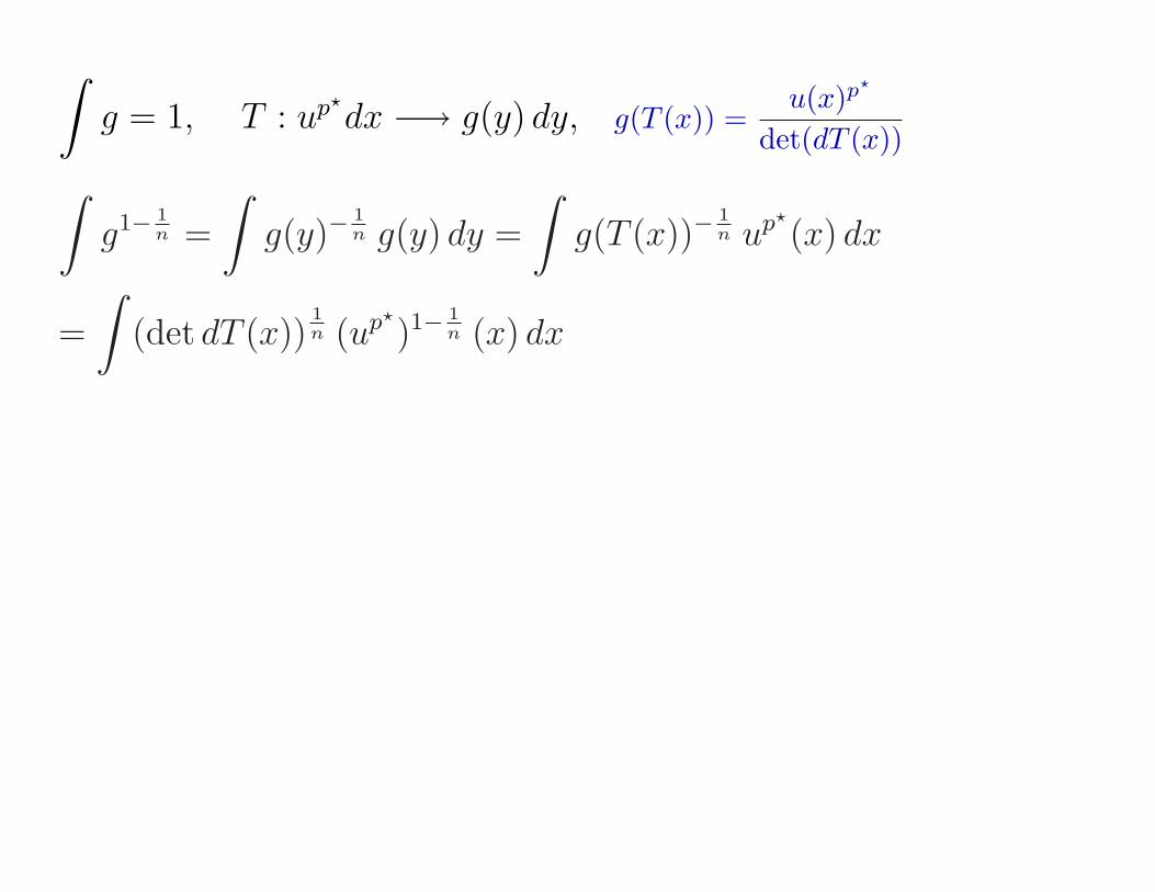
Maintenant prouvons Sobolev (Cordero–Nazaret–V 2004)
Rn, 1 < p < n,
(∫
|u|p⋆
)1/p⋆
≤ S(n, p)
(∫
|∇u|p)1/p
p⋆ =np
n − p
Sans perte de generalite u ≥ 0 et∫
up⋆
= 1: devient
0 < K ≤(∫
Rn
|∇u|p)1/p

∫
g = 1, T : up⋆
dx −→ g(y) dy, g(T (x)) =u(x)p
⋆
det(dT (x))

∫
g = 1, T : up⋆
dx −→ g(y) dy, g(T (x)) =u(x)p
⋆
det(dT (x))
∫
g1− 1n =
∫
g(y)−1n g(y) dy =
∫
g(T (x))−1n up⋆
(x) dx
∫
g = 1, T : up⋆
dx −→ g(y) dy, g(T (x)) =u(x)p
⋆
det(dT (x))
∫
g1− 1n =
∫
g(y)−1n g(y) dy =
∫
g(T (x))−1n up⋆
(x) dx
=
∫
(det dT (x))1n (up⋆
)1− 1n (x) dx

∫
g = 1, T : up⋆
dx −→ g(y) dy, g(T (x)) =u(x)p
⋆
det(dT (x))
∫
g1− 1n =
∫
g(y)−1n g(y) dy =
∫
g(T (x))−1n up⋆
(x) dx
=
∫
(det dT (x))1n (up⋆
)1− 1n (x) dx
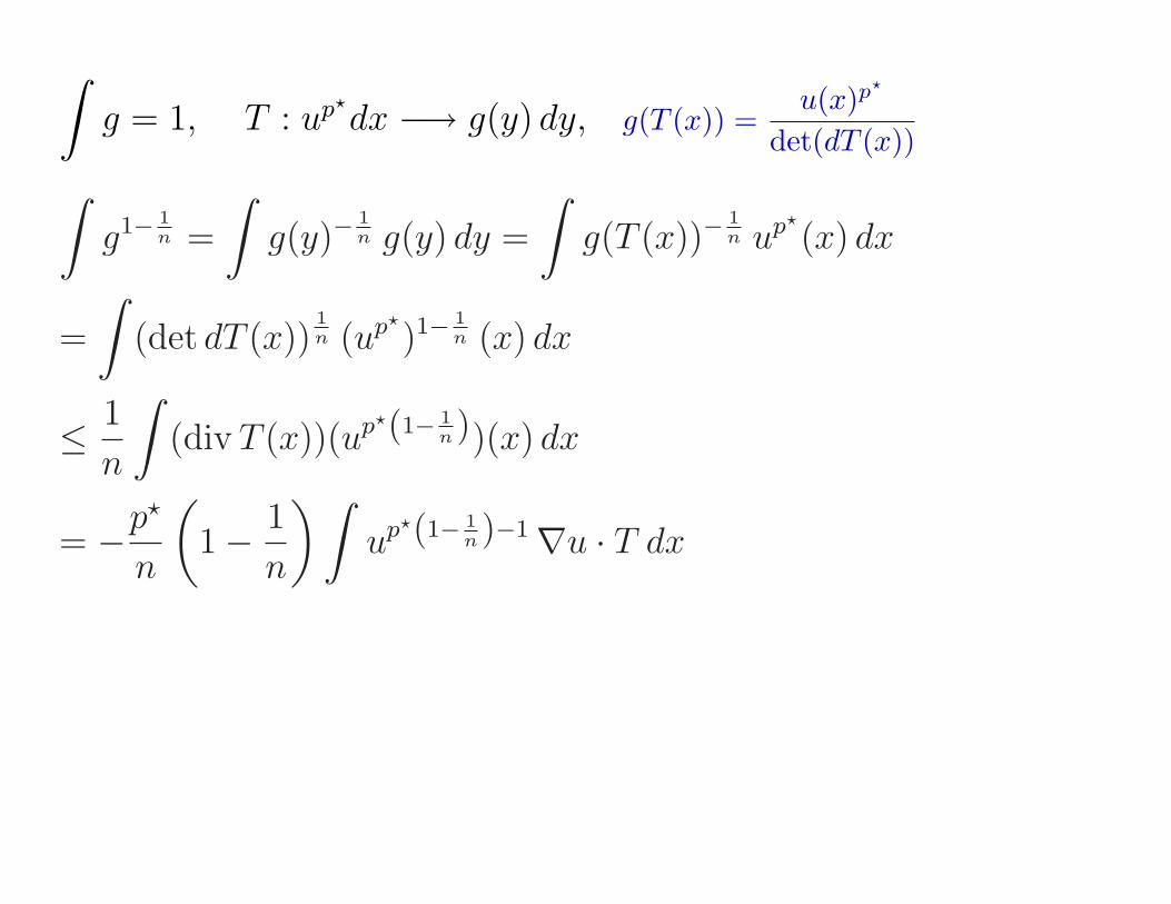
≤ 1
n
∫
(div T (x))(up⋆(1− 1n))(x) dx
∫
g = 1, T : up⋆
dx −→ g(y) dy, g(T (x)) =u(x)p
⋆
det(dT (x))
∫
g1− 1n =
∫
g(y)−1n g(y) dy =
∫
g(T (x))−1n up⋆
(x) dx
=
∫
(det dT (x))1n (up⋆
)1− 1n (x) dx
≤ 1
n
∫
(div T (x))(up⋆(1− 1n))(x) dx
= −p⋆
n
(
1 − 1
n
)∫
up⋆(1− 1n)−1 ∇u · T dx

∫
g = 1, T : up⋆
dx −→ g(y) dy, g(T (x)) =u(x)p
⋆
det(dT (x))
∫
g1− 1n =
∫
g(y)−1n g(y) dy =
∫
g(T (x))−1n up⋆
(x) dx
=
∫
(det dT (x))1n (up⋆
)1− 1n (x) dx
≤ 1
n
∫
(div T (x))(up⋆(1− 1n))(x) dx
= −p⋆
n
(
1 − 1
n
)∫
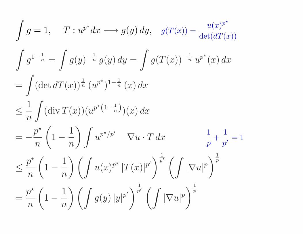
up⋆/p′ ∇u · T dx1
p+
1
p′= 1

∫
g = 1, T : up⋆
dx −→ g(y) dy, g(T (x)) =u(x)p
⋆
det(dT (x))
∫
g1− 1n =
∫
g(y)−1n g(y) dy =
∫
g(T (x))−1n up⋆
(x) dx
=
∫
(det dT (x))1n (up⋆
)1− 1n (x) dx
≤ 1
n
∫
(div T (x))(up⋆(1− 1n))(x) dx
= −p⋆
n
(
1 − 1
n
)∫
up⋆/p′ ∇u · T dx1
p+
1
p′= 1
≤ p⋆
n
(
1 − 1
n
)(∫
u(x)p⋆ |T (x)|p′)
1
p′(∫
|∇u|p)
1p
∫
g = 1, T : up⋆
dx −→ g(y) dy, g(T (x)) =u(x)p
⋆
det(dT (x))
∫
g1− 1n =
∫
g(y)−1n g(y) dy =
∫
g(T (x))−1n up⋆
(x) dx
=
∫
(det dT (x))1n (up⋆
)1− 1n (x) dx
≤ 1
n
∫
(div T (x))(up⋆(1− 1n))(x) dx
= −p⋆
n
(
1 − 1
n
)∫
up⋆/p′ ∇u · T dx1
p+
1
p′= 1
≤ p⋆
n
(
1 − 1
n
)(∫
u(x)p⋆ |T (x)|p′)
1
p′(∫
|∇u|p)
1p
=p⋆
n
(
1 − 1
n
)(∫
g(y) |y|p′)
1
p′(∫
|∇u|p)
1p
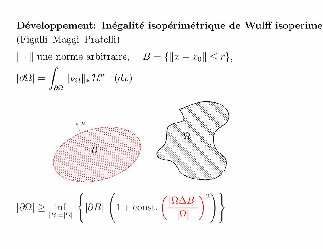
Developpement: Inegalite isoperimetrique de Wulff isoperimetric
(Figalli–Maggi–Pratelli)
‖ · ‖ une norme arbitraire, B = ‖x − x0‖ ≤ r,
|∂Ω| =
∫
∂Ω
‖νΩ‖∗Hn−1(dx)
ν
Ω
B
|∂Ω| ≥ inf|B|=|Ω|
|∂B|(
1 + const.
( |Ω∆B||Ω|
)2)

Autres applications inattendues (20 dernieres annees)
• mecanique des fluides incompressibles (Brenier)
• mesures invariantes syst. dynamiques (Mather)
• equations semigeostrophiques (Cullen)
• equation de Monge–Ampere (Brenier, Caffarelli)
• equation de Boltzmann (Tanaka)
• ecroulement des piles de sable (Prigozhin)
• conception de reflecteurs et lentilles (Oliker, Wang)
• mise en correspondance d’images (Tannenbaum)
• modelisation de bassins d’irrigation (Santambrogio)
• reconstruction de l’univers “initial” (Frisch)
• etc.
..............................................................
A reconstruction of the initialconditions of the Universe byoptimal mass transportationUriel Frisch*, Sabino Matarrese†, Roya Mohayaee‡*& Andrei Sobolevski§*
* CNRS, UMR 6529, Observatoire de la Cote d’Azur, BP 4229, 06304 NiceCedex 4, France† Dipartimento di Fisica “G. Galilei” and INFN, Sezione di Padova,via Marzolo 8, 35131-Padova, Italy‡ Dipartimento di Fisica, Universita Degli Studi di Roma “La Sapienza”,P. le A. Moro 5, 00185-Roma, Italy§ Department of Physics, M V Lomonossov University, 119899-Moscow, Russia
.............................................................................................................................................................................
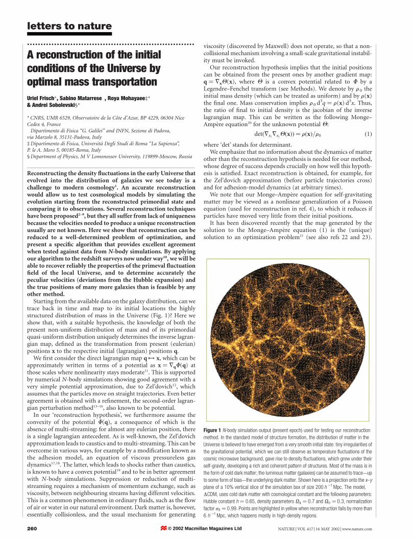
Reconstructing the density fluctuations in the early Universe thatevolved into the distribution of galaxies we see today is achallenge to modern cosmology1. An accurate reconstructionwould allow us to test cosmological models by simulating theevolution starting from the reconstructed primordial state andcomparing it to observations. Several reconstruction techniqueshave been proposed2–9, but they all suffer from lack of uniquenessbecause the velocities needed to produce a unique reconstructionusually are not known. Here we show that reconstruction can bereduced to a well-determined problem of optimization, andpresent a specific algorithm that provides excellent agreementwhen tested against data from N-body simulations. By applyingour algorithm to the redshift surveys now under way10, we will beable to recover reliably the properties of the primeval fluctuationfield of the local Universe, and to determine accurately thepeculiar velocities (deviations from the Hubble expansion) andthe true positions of many more galaxies than is feasible by anyother method.
Starting from the available data on the galaxy distribution, can wetrace back in time and map to its initial locations the highlystructured distribution of mass in the Universe (Fig. 1)? Here weshow that, with a suitable hypothesis, the knowledge of both thepresent non-uniform distribution of mass and of its primordialquasi-uniform distribution uniquely determines the inverse lagran-gian map, defined as the transformation from present (eulerian)positions x to the respective initial (lagrangian) positions q.
We first consider the direct lagrangian map q 7! x, which can beapproximately written in terms of a potential as x ¼ 7qF(q) atthose scales where nonlinearity stays moderate11. This is supportedby numerical N-body simulations showing good agreement with avery simple potential approximation, due to Zel’dovich12, whichassumes that the particles move on straight trajectories. Even betteragreement is obtained with a refinement, the second-order lagran-gian perturbation method13–16, also known to be potential.
In our ‘reconstruction hypothesis’, we furthermore assume theconvexity of the potential F(q), a consequence of which is theabsence of multi-streaming: for almost any eulerian position, thereis a single lagrangian antecedent. As is well-known, the Zel’dovichapproximation leads to caustics and to multi-streaming. This can beovercome in various ways, for example by a modification known asthe adhesion model, an equation of viscous pressureless gasdynamics17,18. The latter, which leads to shocks rather than caustics,is known to have a convex potential19 and to be in better agreementwith N-body simulations. Suppression or reduction of multi-streaming requires a mechanism of momentum exchange, such asviscosity, between neighbouring streams having different velocities.This is a common phenomenon in ordinary fluids, such as the flowof air or water in our natural environment. Dark matter is, however,essentially collisionless, and the usual mechanism for generating
viscosity (discovered by Maxwell) does not operate, so that a non-collisional mechanism involving a small-scale gravitational instabil-ity must be invoked.
Our reconstruction hypothesis implies that the initial positionscan be obtained from the present ones by another gradient map:q ¼ 7xQ(x), where Q is a convex potential related to F by aLegendre–Fenchel transform (see Methods). We denote by r0 theinitial mass density (which can be treated as uniform) and by r(x)the final one. Mass conservation implies r0 d3q ¼ r(x) d3x. Thus,the ratio of final to initial density is the jacobian of the inverselagrangian map. This can be written as the following Monge–Ampere equation20 for the unknown potential Q:
detð7xi7xj
QðxÞÞ ¼ rðxÞ=r0 ð1Þ
where ‘det’ stands for determinant.We emphasize that no information about the dynamics of matter
other than the reconstruction hypothesis is needed for our method,whose degree of success depends crucially on how well this hypoth-esis is satisfied. Exact reconstruction is obtained, for example, forthe Zel’dovich approximation (before particle trajectories cross)and for adhesion-model dynamics (at arbitrary times).
We note that our Monge–Ampere equation for self-gravitatingmatter may be viewed as a nonlinear generalization of a Poissonequation (used for reconstruction in ref. 4), to which it reduces ifparticles have moved very little from their initial positions.
It has been discovered recently that the map generated by thesolution to the Monge–Ampere equation (1) is the (unique)solution to an optimization problem21 (see also refs 22 and 23).
Figure 1 N-body simulation output (present epoch) used for testing our reconstruction
method. In the standard model of structure formation, the distribution of matter in the
Universe is believed to have emerged from a very smooth initial state: tiny irregularities of
the gravitational potential, which we can still observe as temperature fluctuations of the
cosmic microwave background, gave rise to density fluctuations, which grew under their
self-gravity, developing a rich and coherent pattern of structures. Most of the mass is in
the form of cold dark matter; the luminous matter (galaxies) can be assumed to trace—up
to some form of bias—the underlying dark matter. Shown here is a projection onto the x–y
plane of a 10% vertical slice of the simulation box of size 200 h 21 Mpc. The model,
LCDM, uses cold dark matter with cosmological constant and the following parameters:
Hubble constant h ¼ 0.65, density parameters QL ¼ 0:7 and Qm ¼ 0:3, normalization
factor j8 ¼ 0:99. Points are highlighted in yellow when reconstruction fails by more than
6 h 21 Mpc, which happens mostly in high-density regions.
letters to nature
NATURE | VOL 417 | 16 MAY 2002 | www.nature.com260 © 2002 Macmillan Magazines Ltd
This is the ‘mass transportation’ problem of Monge and Kantor-ovich24,25, in which one seeks the map x 7! q that minimizes thequadratic ‘cost’ function:
I ¼
ðq
r0jx 2 qj2
d3q¼
ðx
rðxÞjx 2 qj2
d3x ð2Þ
Note that x ¼ q is forbidden: as the initial and final density fields r0
and r(x) are prescribed, there is a constraint on the jacobian of themap (see Methods).
Next, we take into account that information on the massdistribution is provided in the form of N discrete particles both insimulations and when handling observational data from galaxysurveys. The cost minimization then becomes what is known inoptimization theory as the assignment problem: find the uniqueone-to-one pairing of a set of N initial points q j and N final points x i
that minimizes Idiscr ¼PN
i¼1jx i 2 qjðiÞj2: An immediate conse-
quence is that, for any subset of k pairs of initial and final points(2 # k # N), the contribution of these points to the cost functionshould not decrease under arbitrary permutations of initial points.This property is known to be equivalent to having a lagrangian mapthat is the gradient of a convex function26.
If we restrict ourselves to interchanging just pairs (k ¼ 2), themap is said to be monotonic, a condition not equivalent tominimization of the cost function (except in one dimension). Inref. 5, a method of reconstruction called the path interchangeZel’dovich approximation (PIZA) is introduced, which uses thesame quadratic cost function (obtained by applying a minimum-action argument within the framework of the Zel’dovich approxi-mation). In PIZA, a randomly chosen tentative correspondencebetween initial and final points is successively improved by swap-ping pairs of initial particles whenever this decreases the cost
function. Eventually, a monotonic map is obtained that usuallydoes not minimize the cost. This explains the non-uniqueness ofPIZA reconstruction (also noticed in ref. 8).
There are, however, known deterministic strategies for the assign-ment problem that give the correct unique solution; their complex-ity (dependence on N of the number of operations needed) is closeto N 3 for arbitrary cost functions, but can be sharply reduced whenthe cost function is quadratic. Combining the organization of datataken from Henon’s mechanical analogue machine (see ref. 27, andhttp://www.obs-nice.fr/etc7/henon.pdf) for solving the assignmentproblem with the dual simplex method of Balinski28, we havedesigned an algorithm that gives the optimal assignment forabout 20,000 particles in a few hours of CPU time on a fast Alphamachine. For historical reasons, we call our approach Monge–Ampere–Kantorovich or MAK (see Methods). Details of the algor-ithms will be given elsewhere; we merely note that, when workingwith the catalogues of several hundred thousand galaxies that areexpected within a few years, a direct application of the assignmentalgorithm in its present state could require unreasonable compu-tational resources. A mixed strategy can however be used, in whichthe assignment problem is solved on a coarse grid while, on smallerscales, the Monge–Ampere equation (1) is solved by a relaxationtechnique (adapted from ref. 23).
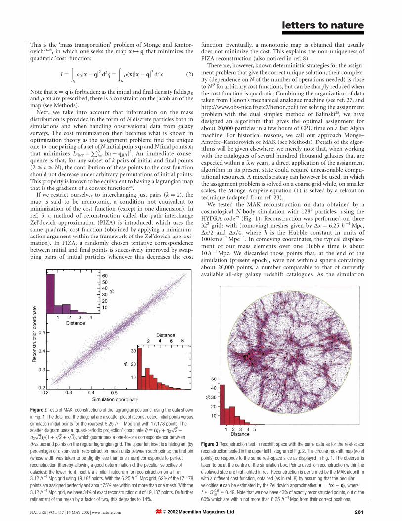
We tested the MAK reconstruction on data obtained by acosmological N-body simulation with 1283 particles, using theHYDRA code29 (Fig. 1). Reconstruction was performed on three323 grids with (comoving) meshes given by Dx ¼ 6.25 h21 Mpc,Dx/2 and Dx/4, where h is the Hubble constant in units of100 km s21 Mpc21. In comoving coordinates, the typical displace-ment of our mass elements over one Hubble time is about10 h21 Mpc. We discarded those points that, at the end of thesimulation (present epoch), were not within a sphere containingabout 20,000 points, a number comparable to that of currentlyavailable all-sky galaxy redshift catalogues. As the simulation
Figure 2 Tests of MAK reconstructions of the lagrangian positions, using the data shown
in Fig. 1. The dots near the diagonal are a scatter plot of reconstructed initial points versus
simulation initial points for the coarsest 6.25 h 21 Mpc grid with 17,178 points. The
scatter diagram uses a ‘quasi-periodic projection’ coordinate ~q ; ðq1þ q2
ffiffiffi2pþ
q3
ffiffiffi3pÞ=ð1þ
ffiffiffi2pþ
ffiffiffi3pÞ; which guarantees a one-to-one correspondence between
q-values and points on the regular lagrangian grid. The upper left inset is a histogram (by
percentage) of distances in reconstruction mesh units between such points; the first bin
(whose width was taken to be slightly less than one mesh) corresponds to perfect
reconstruction (thereby allowing a good determination of the peculiar velocities of
galaxies); the lower right inset is a similar histogram for reconstruction on a finer
3.12 h 21 Mpc grid using 19,187 points. With the 6.25 h 21 Mpc grid, 62% of the 17,178
points are assigned perfectly and about 75% are within not more than one mesh. With the
3.12 h 21 Mpc grid, we have 34% of exact reconstruction out of 19,187 points. On further
refinement of the mesh by a factor of two, this degrades to 14%.
Figure 3 Reconstruction test in redshift space with the same data as for the real-space
reconstruction tested in the upper left histogram of Fig. 2. The circular redshift map (violet
points) corresponds to the same real-space slice as displayed in Fig. 1. The observer is
taken to be at the centre of the simulation box. Points used for reconstruction within the
displayed slice are highlighted in red. Reconstruction is performed by the MAK algorithm
with a different cost function, obtained (as in ref. 8) by assuming that the peculiar
velocities v can be estimated by the Zel’dovich approximation: v ¼ f (x 2 q), where
f < Q 0:6m < 0:49: Note that we now have 43% of exactly reconstructed points, out of the
60% which are within not more than 6.25 h 21 Mpc from their correct positions.
letters to nature
NATURE | VOL 417 | 16 MAY 2002 | www.nature.com 261© 2002 Macmillan Magazines Ltd

assumes periodic boundary conditions, we also took into accountperiodicity when calculating the distance between pairs of points.The MAK reconstructions were used to generate a scatter diagramand various histograms allowing comparisons of simulation andreconstructed lagrangian points (Fig. 2). The results demonstratethe essentially potential character of the lagrangian map above,6 h21 Mpc (within the given cosmological model).
We also performed PIZA reconstructions on the coarsest grid, andobtained typically 30–40% exactly reconstructed points, but severenon-uniqueness: for two different seeds of the random generator,only about half of the exactly reconstructed points were the same.
When reconstructing from observational data, in redshift space(Fig. 3), the galaxies appear displaced radially (as seen by theobserver) by an amount proportional to the radial component ofthe peculiar velocity. We thus performed another reconstruction,with an accordingly modified cost function, that led to somewhatdegraded results (Fig. 3) but at the same time provided anapproximate determination of peculiar velocities. More-accuratedetermination of peculiar velocities can be done using second-orderlagrangian perturbation theory. The effect of the catalogue selectionfunction can be handled by standard techniques; for instance, onecan assign each galaxy a ‘mass’ inversely proportional to thecatalogue selection function8,9.
What is the smallest length scale at which an optimizationalgorithm such as MAK can be expected to give a unique andreliable reconstruction? The key ingredient here is the simultaneousknowledge of the initial and present mass density fields. MAK-typereconstruction (with a suitable cost based on the equation of a self-gravitating fluid) should therefore be possible down to scalescomparable to the thickness of collapsed structures, below whichthe hydrodynamical description ceases to be meaningful.
The fact that MAK guarantees a unique solution, and that ourpresent reconstruction hypothesis proved to be very faithful downto 6.5 h21 Mpc, makes our method very promising for the analysisof galaxy redshift surveys10. Reconstruction of the primordialpositions and velocities of matter will allow us to test the gaussiannature of the primordial perturbations and the self-consistency ofcosmological hypotheses, such as the choice of the global cosmo-logical parameters and the assumed biasing scheme. By obtaining apoint-by-point reconstruction of the specific realization thatdescribes the observed patch of our Universe, we could distinguishbetween universal properties and the influence of the large-scaleenvironment on the galaxy formation process. Moreover, recon-struction would open a new window not only onto the past but alsointo the present Universe: it would enable us to determine thepeculiar velocities of a very large number of galaxies, using theirpositions in redshift catalogues. A
MethodsMonge–Ampere equationThe lagrangian map q 7! x is taken to be the gradient of a convex potential F(q); thereforeits inverse x 7! q also has a potential representation q ¼ 7xQ(x), where Q(x) is again aconvex function; the two potentials are Legendre–Fenchel transforms of each other (seepages 61–65 in ref. 30):
QðxÞ ¼q
max½qx 2 FðqÞ; FðqÞ ¼x
max½xq 2 QðxÞ ð3Þ
The potential Q satisfies the Monge–Ampere equation (1), written for the first time byAmpere20 by exploiting the property of the Legendre transformation. Note that within themore restricted framework of the Zel’dovich approximation, Q differs just by a quadraticadditive term from the eulerian velocity potential19.
Quadratic cost functionTo show that the quadratic cost minimization leads to the Monge–Ampere equation, wedefine the displacement field y(x) ; x 2 q(x) and perform a variation dy(x) to obtain, tolowest order, the variation of the cost function dI ¼
Ðx 2yðxÞðrðxÞdyÞd3x: The condition
that the eulerian density remains unchanged, which constrains the variation, is expressedas 7x(r(x)dy(x)) ¼ 0. By a simple Lagrange multiplier argument, this implies that y
must be a gradient of some function of x; thus, q ¼ x 2 y ¼ 7xQ(x). Furthermore,should Q be non-convex and thus lead to multi-streaming, this would prevent thelagrangian map from being optimal.
History of mass transportationMonge24 posed the following problem: how to optimally move material from one place toanother, knowing only its initial and final spatial distributions, the cost being a prescribedfunction of the distance travelled by ‘molecules’ of material (a linear function in Monge’soriginal work). Kantorovich25 showed that Monge’s query was an instance of the linearprogramming problem, and developed for it a theory that found numerous applications ineconomics and applied mathematics.
Received 26 September 2001; accepted 5 April 2002.
1. Narayanan, V. K. & Croft, R. A. Recovering the primordial density fluctuations: a comparison of
methods. Astrophys. J. 515, 471–486 (1999).
2. Peebles, P. J. E. Tracing galaxy orbits back in time. Astrophys. J. 344, L53–L56 (1989).
3. Weinberg, D. H. Reconstructing primordial density fluctuations—I. Method. Mon. Not. R. Astron. Soc.
254, 315–342 (1992).
4. Nusser, A. & Dekel, A. Tracing large-scale fluctuations back in time. Astrophys. J. 391, 443–452 (1992).
5. Croft, R. A. & Gaztanaga, E. Reconstruction of cosmological density and velocity fields in the
Lagrangian Zel’dovich approximation. Mon. Not. R. Astron. Soc. 285, 793–805 (1997).
6. Nusser, A. & Branchini, E. On the least action principle in cosmology. Mon. Not. R. Astron. Soc. 313,
587–595 (2000).
7. Goldberg, D. M. & Spergel, D. N. Using perturbative least action to recover cosmological initial
conditions. Astrophys. J. 544, 21–29 (2000).
8. Valentine, H., Saunders, W. & Taylor, A. Reconstructing the IRAS point source catalog redshift survey
with a generalized PIZA. Mon. Not. R. Astron. Soc. 319, L13–L17 (2000).
9. Branchini, E., Eldar, A. & Nusser, A. Peculiar velocity reconstruction with fast action method: tests on
mock redshift surveys. Mon. Not. R. Astron. Soc. (submitted); preprint astro-ph/0110618 at
khttp://xxx.lanl.govl (2001).
10. Frieman, J. A. & Szalay, A. S. Large-scale structure: entering the precision era. Phys. Rep. 333–334,
215–232 (2000).
11. Bertschinger, E. & Dekel, A. Recovering the full velocity and density fields from large-scale redshift-
distance samples. Astrophys. J. 336, L5–L8 (1989).
12. Zel’dovich, Ya. B. Gravitational instability: an approximate theory for large density perturbations.
Astron. Astrophys. 5, 84–89 (1970).
13. Moutarde, F., Alimi, J.-M., Bouchet, F. R., Pellat, R. & Ramani, A. Precollapse scale invariance in
gravitational instability. Astrophys. J. 382, 377–381 (1991).
14. Buchert, T. Lagrangian theory of gravitational instability of Friedman-Lemaitre cosmologies and the
Zel’dovich approximation. Mon. Not. R. Astron. Soc. 254, 729–737 (1992).
15. Munshi, D., Sahni, V. & Starobinsky, A. Nonlinear approximations to gravitational instability: a
comparison in the quasi-linear regime. Astrophys. J. 436, 517–527 (1994).
16. Catelan, P. Lagrangian dynamics in non-flat universes and non-linear gravitational evolution. Mon.
Not. R. Astron. Soc. 276, 115–124 (1995).
17. Gurbatov, S. & Saichev, A. I. Probability distribution and spectra of potential hydrodynamic
turbulence. Radiophys. Quant. Electr. 27, 303–313 (1984).
18. Shandarin, S. F. & Zel’dovich, Ya. B. The large-scale structure of the universe: turbulence,
intermittency, structures in a self-gravitating medium. Rev. Mod. Phys. 61, 185–220 (1989).
19. Vergassola, M., Dubrulle, B., Frisch, U. & Noullez, A. Burgers’ equation, Devil’s stair-cases and the
mass distribution for large-scale structures. Astron. Astrophys. 289, 325–356 (1994).
20. Ampere, A.-M. Memoire concernant l’Application de la Theorie exposee dans le XVIIe Cahier du
Journal de l’Ecole Polytechnique, a l’Integration des Equations aux differentielles partielles du premier
et du second ordre. J. Ecole. R. Polytech. 11, 1–188 (1820).
21. Brenier, Y. Decomposition polaire et rearrangement monotone des champs de vecteurs. C.R. Acad. Sci.
305, 805–808 (1987).
22. Gangbo, W. & McCann, R. J. The geometry of optimal transportation. Acta Math. 177, 113–161 (1996).
23. Benamou, J.-D. & Brenier, Y. The optimal time-continuous mass transport problem and its
augmented Lagrangian numerical resolution. Numer. Math. 84, 375–393 (2000) also at khttp://
www.inria.fr/rrrt/rr-3356.htmll.24. Monge, G. Memoire sur la theorie des deblais et des remblais. Hist. Acad. R. Sci. Paris, 666–704 (1781).
25. Kantorovich, L. On the translocation of masses. C.R. Acad. Sci. URSS 37, 199–201 (1942).
26. Rockafellar, R. T. Convex Analysis (Princeton Univ. Press, 1970).
27. Henon, M. A mechanical model for the transportation problem. C.R. Acad. Sci. 321, 741–745 (1995).
28. Balinski, M. L. A competitive (dual) simplex method for the assignment problem. Math. Program. 34,
125–141 (1986).
29. Couchman, H. M. P., Thomas, P. A. & Pearce, F. R. Hydra: an adaptive-mesh implementation of P3M-
SPH. Astrophys. J. 452, 797–813 (1995).
30. Arnold, V. I. Mathematical Methods of Classical Mechanics (Springer, Berlin, 1978).
AcknowledgementsSpecial thanks are due to E. Branchini (observational and conceptual aspects), Y. Brenier(mathematical aspects) and M. Henon (algorithmic aspects and the handing of spatialperiodicity and of scatter plots). We also thank J. Bec, H. Frisch, B. Gladman,L. Moscardini, A. Noullez, C. Porciani, M. Rees, E. Spiegel, A. Starobinsky and P. Thomasfor comments. This work was supported by the BQR program of Observatoire de la Coted’Azur, by the TMR program of the European Union (U.F., R.M.), by MIUR (S.M.), by theFrench Ministry of Education, the McDonnel Foundation, the Russian RFBR and INTAS(A.S.).
Competing interests statement
The authors declare that they have no competing financial interests.
Correspondence and requests for materials should be addressed to U.F.
(e-mail: [email protected]).
letters to nature
NATURE | VOL 417 | 16 MAY 2002 | www.nature.com262 © 2002 Macmillan Magazines Ltd

Rappels de base de geometrie riemannienne
• espace tangent TxM muni d’un produit scalaire gx =
metrique
• |u |x =√
gx(u, u)
• longueur d’une courbe L(γ) =
∫ 1
0
|γ(t)|γ(t) dt
• distance: d(x, y) = inf
L(γ); γ(0) = x, γ(1) = y
• geodesique: γ tq L(γ) = d(
γ(0), γ(1))
Par defaut parametree a vitesse constante
• volume: mesure canonique generalisant Lebesgue,
fonction croissante de distance

Jordan–Kinderlehrer–Otto (1998)
Sur M variete riemannienne compacte (or M = Rn)
il y a un lien entre
• equation de la chaleur/Fourier∂ρ
∂t= ∆ρ sur M
• fonctionnelle H de Boltzmann: H(ρ) =
∫
ρ log ρ
• transport optimal C(µ, ν) = infT#µ=ν
∫
d(
x, T (x))2
µ(dx)

Comment resoudre Fourier par Monge?
Schema flot gradient non orthodoxe. Discretise en temps.
Du temps t au temps t + ∆t: Etant donne ρ(t), on
cherche ρ(t + ∆t) = minimiseur de H(ρ) +C(ρ(t), ρ)
2 ∆t
L’entropie −H = −∫
ρ log ρ augmente avec t (bien sur)

Comment resoudre Fourier par Monge?
Schema flot gradient non orthodoxe. Discretise en temps.
Du temps t au temps t + ∆t: Etant donne ρ(t), on
cherche ρ(t + ∆t) = minimiseur de H(ρ) +C(ρ(t), ρ)
2 ∆t
L’entropie −H = −∫
ρ log ρ augmente avec t (bien sur)
Interpolation le long du transport optimal
L’interpolation µt entre µ0 et µ1 est obtenue en arretant
la geodesique au temps t: Tt(x) est la trajectoire de
T0(x) = x a T1(x) = T (x)
µt = (Tt)#µ0 C’est une geodesique dans l’espace des
measures de probabilite, muni de la distance√
C(µ, ν)
Quel est le comportement de H en fct de t?

Courbure sectionnelle
Soient u, v ∈ TxM des vecteurs unitaires orthogonaux.
κ(u, v) mesure la divergence “extra-euclidienne” des
geodesiques: d(γu(t), γv(t)) =√
2 t(
1 − κ
12t2 + O(t4)
)
v
δ(t)
t
u

Courbure sectionnelle
Soient u, v ∈ TxM des vecteurs unitaires orthogonaux.
κ(u, v) mesure la divergence “extra-euclidienne” des
geodesiques: d(γu(t), γv(t)) =√
2 t(
1 − κ
12t2 + O(t4)
)
v
δ(t)
t
u
Courbure “de Ricci” = “sectionnelle moyenne”
(e, e2, . . . , en) orthonormal, alors Ric(e) :=n∑
j=2
κ(e, ej)
Ceci s’etend a une forme quadratique
(exprimee en fct des derivees secondes de la metrique g)

Relation entre transport et Ricci
Ric ≥ 0
si et seulement si
H(µt) =
∫
ρt log ρt dx est une fonction convexe de t
ρt =dµt
dx
(convexite le long des geodesiques du transport optimal!)

Courbure de Ricci et distortion
the observerlocation of
the light source looks likehow the observer thinks
the light source
by curvature effects
geodesics are distorted
A cause de la courbure positive, l’observateur surestime la surface
de la source lumineuse; en courbure negative ce serait le contraire.
[Coefficients de distortion toujours ≥ 1] ⇐⇒ [Ric ≥ 0]

L’experience du gaz paresseux
t = 1
t = 0
t = 1/2
t = 0 t = 1
S = −
Z
ρ log ρ

Analytique vs. Synthetique
Def. (i) ϕ ∈ C2(Rn; R) est convexe si pour tout x,
∇2ϕ(x) ≥ 0
Def. (ii) ϕ : Rn → R est convexe si pour tous x, y, t,
ϕ(
(1 − t)x + ty)
≤ (1 − t) ϕ(x) + t ϕ(y)
(i): simple, local, effectif
(ii): utile, general, stable

Espaces metriques de courbure sectionnelle positive
(Cartan–Alexandrov–Toponogov)
κ ≥ 0
⇐⇒Triangles plus gras que triangles euclidiens
y0z0
z
x0x
y
−→ espaces d’Alexandrov

Espaces metriques de courbure sectionnelle positive
(Cartan–Alexandrov–Toponogov)
κ ≥ 0
⇐⇒Triangles plus gras que triangles euclidiens
y0z0
z
x0
y
x
−→ espaces d’Alexandrov

Exemple: cone
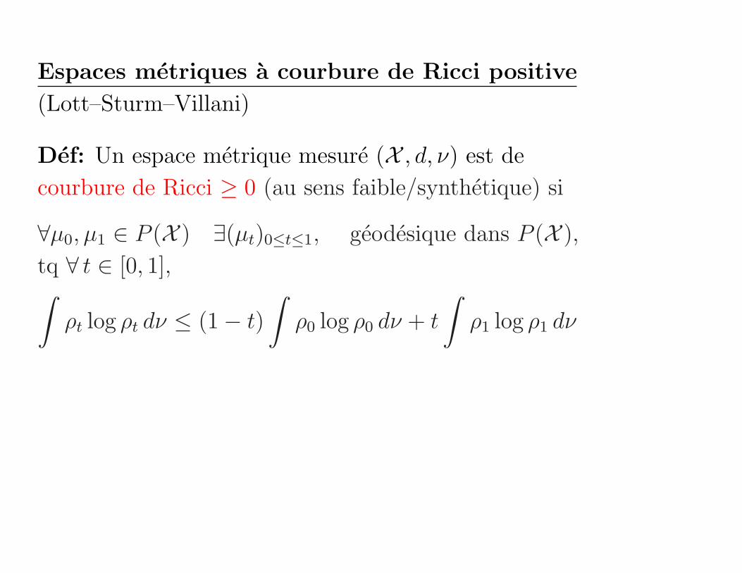
Espaces metriques a courbure de Ricci positive
(Lott–Sturm–Villani)
Def: Un espace metrique mesure (X , d, ν) est de
courbure de Ricci ≥ 0 (au sens faible/synthetique) si
∀µ0, µ1 ∈ P (X ) ∃(µt)0≤t≤1, geodesique dans P (X ),
tq ∀ t ∈ [0, 1],∫
ρt log ρt dν ≤ (1 − t)
∫
ρ0 log ρ0 dν + t
∫
ρ1 log ρ1 dν

Espaces metriques a courbure de Ricci positive
(Lott–Sturm–Villani)
Def: Un espace metrique mesure (X , d, ν) est de
courbure de Ricci ≥ 0 (au sens faible/synthetique) si
∀µ0, µ1 ∈ P (X ) ∃(µt)0≤t≤1, geodesique dans P (X ),
tq ∀ t ∈ [0, 1],∫
ρt log ρt dν ≤ (1 − t)
∫
ρ0 log ρ0 dν + t
∫
ρ1 log ρ1 dν
Compatibilite
La definition faible coıncide avec la definition habituelle
si l’espace est lisse (variete riemannienne)
Consequences analytiques
Par exemple Ric ≥ 0 au sens faible avec dimension N
implique une inegalite de Sobolev

Stabilite
Def: (Xk, dk, νk)k∈N converge vers (X , d, ν) dans la
topologie de Gromov–Hausdorff mesuree s’il y a
convergence des distances et du volume. Plus
precisement s’il existe fk : Xk → X
∣
∣d(fk(x), fk(y)) − dk(x, y)∣
∣ ≤ εk → 0
∀x ∈ X, d(
x, fk(Xk))
≤ εk
(fk)#νk −→ ν faiblement

Stabilite
Def: (Xk, dk, νk)k∈N converge vers (X , d, ν) dans la
topologie de Gromov–Hausdorff mesuree s’il y a
convergence des distances et du volume. Plus
precisement s’il existe fk : Xk → X
∣
∣d(fk(x), fk(y)) − dk(x, y)∣
∣ ≤ εk → 0
∀x ∈ X, d(
x, fk(Xk))
≤ εk
(fk)#νk −→ ν faiblement
Thm: Si (Xk, dk, νk) sat. Ric ≥ 0 alors (X , d, ν) aussi.

Compatibilite metrique (Petrunin 2009)
Si (X , d) est un espace d’Alexandrov compact de
dimension finie avec courbure “sectionnelle” ≥ 0 alors
≥ 0 egalement (X , d, vol) a “Ricci” ≥ 0.
Ceci etablit un lien direct entre
Cartan–Alexandrov–Toponogov et Lott–Sturm–V
et assure la compatibilite des definitions faibles

CONCLUSIONS
Va-et-vient entre
• mathematiques et ingenierie et physique
• analyse et probabilites et geometrie
• synthetique et analytique
• dynamique et variationnel
Les theoremes ne se mettent pas dans des cases....


Strategie de preuve de la stabilite
Etape 1: On reformule la condition “Ric ≥ 0”:
Etant donnees deux mesures de probabilite µ0 et µ1
quelconques, il y a une geodesique (µt)0≤t≤1 dans l’espace
de Wasserstein (P (X ),√
C), t.q.
Hν(µt) ≤ (1 − t) Hν(µ0) + t Hν(µ1)
Step 2: P2(X) est stable sous MGH:
Si fk : Xk → X est une isometrie approchee, alors
(fk)# : P2(Xk) → P2(X)
En combinant avec un argument de compacite, on trouve
une geodesique limite dans l’espace des mesures.

Step 3: Utiliser les proprietes de l’entropie pour passer a
la limite dans l’inegalite
Si U : R+ → R+ est convexe continue, alors
Uν(µ) :=
∫
U
(
dµ
dν
)
dν
est semicontinue inferieurement en µ et ν,
et verifie un principe de contraction:
pour tout f, Uf#ν(f#µ) ≤ Uν(µ)
Conclure que la meme propriete est verifiee dans l’espace
limite, donc Ric ≥ 0.