TRANSPORT COSTS AND TRADE: EMPIRICALEVIDENCE FOR LATINOAMERICAN IMPORTS

FROM THE EUROPEAN UNION

Author(s)

Martínez-Zarzoso, Inmaculada*

Suárez-Burguet, Celestino*

Institution: * Institute of International Economics. Universitat Jaume I, Spain

.

Postal Address and E-mail:

Departamento de Economía, Campus del Riu Sec, 12080-Castellón, Spain.

Emails: martinei@eco.uji.es, celes@eco.uji.es.

Tel: 0034 964728590. Fax: 0034 964728591

* The authors acknowledge the support and collaboration of Proyecto Bancaja-Castellon P-1B92002-11,Proyectos BEC 2002-02083 and SEC 2002-03651 and Proyecto Generalitat Valenciana GV01-129.

2

TRANSPORT COSTS AND TRADE: EMPIRICAL EVIDENCE FOR

LATINOAMERICAN IMPORTS FROM THE EUROPEAN UNION

Abstract

This paper aims to investigate the relationship between trade and transport costs. In previous studies the

cost of transport was considered as an exogenous variable. However, an expanding volume of trade also

reduces the unit cost of transport and therefore, the causal relationship between trade and transport costs

may be operating in both directions. A transport-costs equation is estimated using data on transportation

costs from the International Transport Data Base (BTI). The relationship between transport costs and

trade is then analysed by applying a gravity model for sectoral imports for five South-American Countries

from the European Union. We investigate the endogeneity of the trade and transport cost variables by

estimating simultaneously both equations.

Our results show that, while higher distance and poor importer's infrastructure notably increase transport

costs, a higher volume of trade have the opposite effect, lowering transport costs. Moreover, trade is

significantly deterred by higher transport costs and fostered by cultural similarities.

Key words : transport costs infrastructure imports sectors

JEL classifications: F14

1. Motivation

In this paper, we aim to evaluate the relative importance of different sources of trade

costs, namely, freight rates, economies of scale, poor infrastructure and location in

Latin-American imports from the European Union (EU). Recent liberalisation processes

in Latin America have reduced both tariff and non-tariff barriers considerably. In 1997,

Latin America had an average tariff of 8.4 percent for imports from the EU,

considerably lower than the 34 percent average of 19861. This reduction in artificial

trade barriers has implied that transport costs have become an increasingly important

1 Source: IMF data

3

determinant of trade. In 1998, the average freight rate for Mercosur imports from the

EU was 15 percent 2. Therefore, any additional effort to integrate a country into the

trading system has to consider transport costs.

In most cases we have no direct way of observing trade barriers, and therefore we have

to rely on proxies, indirect measurement and trade modelling in order to assess their

relevance. Hummels (1999) made a significant contribution to the literature by showing

clear evidence of the importance of trade costs. His results suggest that, to some extent,

import choices are made in order to minimise transportation costs.

In our research we introduce two significant novelties. First, we use disaggregated data

on freight rates. Rauch (1999) emphasised that transport costs depend upon the type of

product traded. He showed that search costs are higher for trade in differentiated

products. When aggregated data are used and the composition of trade is not considered,

the effect of transport costs -distance- in trade patterns can be misleading. To our

knowledge, only a few authors have considered disaggregated data, but with different

purposes (e.g. Hummels, 1999; Rauch, 1999).

Second, as stated in Kumar and Hoffmann (2002):

"What appears to be missing in the reviewed literature is a more thorough

consideration of the mutual relationship between trade volumes, transport costs and the

quality of transport services"

We investigate the endogeneity of the transport cost variable by estimating

simultaneously the trade and transport cost equations. We specify an augmented trade

cost equation that adds infrastructure, port efficiency and economies of scale as

explanatory variables. We made use of an infrastructure index constructed in a similar

way to that of Limao and Venables (2001) and also of data on port efficiency from the

Global Competitiveness Report. We apply a gravity model to bilateral trade flows

2 Source: Data Base for International Transport (BTI).

4

between Latin American countries and the European Union in order to investigate to

what extent transport costs are an important determinant of imports and to evaluate the

trade composition effect.

In Section two we discuss the importance of international trade costs for international

trade. Section three presents the different methods used in the recent literature to

measure transportation costs. In Section 4, a transport cost equation is estimated by

using sectoral data. Section 5 presents a variant of the standard gravity model of trade.

Section 6 discusses the results of the empirical application and concludes.

2. The cost of moving goods across countries

A common practice in the literature related to gravity equations has been to proxy

transport costs with the geographical distance between countries. It has been shown that

distance seems to be a good proxy for transport costs at aggregate level. However it is

not clear that this good performance remains at more detailed levels (Hummels,1999).

Venables (2001) classifies the costs of distance into four types. First, the cost of moving

goods internationally (direct shipping costs). Second, searching costs (the cost of

identifying potential trading partners). Third, control and management costs and finally,

the cost of time involved in shipping goods. Hence, when distance is added as a

regressor in gravity models of trade, it is far from clear how the magnitude of the

estimated coefficient should be interpreted. Most research situates the elasticity of

aggregated trade flows with respect to distance in the interval (-0.5, -1.5)3. This shows a

major decrease in trade volumes caused by higher distances. A growing interest has

recently been shown in the study of the "new economics of distance". Researchers argue

that most distance-related costs tend to decrease with the continuous development of

new technologies. However, the empirical literature on gravity models shows that the

3 Coe et al. (2002) report a summary of estimates of distance coefficients obtained recently by differentauthors (page 5).

5

estimated coefficients on distance have been remarkably stable over time. An exception

is Coe et al. (2002). In their non-linear specification of the gravity model the coefficient

estimates of distance clearly decline over time.

Does information technology mark the end of the importance of distance? The answer

to this question is not straightforward. The cost of moving materials using different

modes has changed at different rates across categories without always showing the

expected decrease over time. Only the cost of moving information has steadily declined

(92% between 1960-19984), but the cost of moving goods has not declined continuously

(e.g. the cost of sea transport declined during the 1940's and 1950's but since then there

has been no clear declining trend, Hummels (2001)).

Rauch (1999) identified some of the non-conventional cost of trade associated with

search for the case of different types of goods. He claimed that these informational costs

fall relatively on differentiated goods. He focussed on the effects of distance and

common language/colonial ties in trade of three types of goods: those traded on

organised exchanges, those possessing reference prices and all other commodities. The

author presented evidence that shows that proximity and common language/colonial ties

are more important for differentiated products than for products traded on organised

exchanges in matching international buyers and sellers.

Hummels (1999) classified the trade costs implied by trade flows into three different

categories: explicit measured costs, given by tariffs and freight rates; costs associated

with common proxy variables such as distance, sharing a language, sharing a border or

being and island, and implied but unmeasured trade costs, given by geographical

position, cultural ties or political stability. His results indicated that explicit measured

costs were the most important component. He offered alternative explanations for the

costs associated with distance and adjacency effects based on direct trade barriers, on

6

endogenous production responses and on preferences. However, the regression results

do not allow the possibility of disentangling among the various interpretations.

Hummels (1999) found that adjacency and distance effects were rarely relevant when

interpreted directly as trade barriers. However, when interpreted as a price premia these

effects were important in approximately 75% of the products. Moreover, the author

gave a tentative interpretation of the residuals of the import demand equations in terms

of the willingness to pay for preferred varieties, assuming that they are unmeasured

trade costs. As he pointed out, this interpretation implies that the estimation suffers from

omitted variables and also from the biases these variables may induce in the estimated

coefficients. Hummels’ concluded that freight rates at disaggregated level are higher

than aggregated rates and vary considerably among exporters and among products,

which suggests that import choices are made in order to minimise transport costs. He

also claimed that the channels through which trade barriers affect trade volumes remain

unclear and are a subject for further research. Finally, he offered a complete

characterisation of the trade costs implied by trade flows, by establishing a fresh

classification of those costs into the three components mentioned above. In the same

vein as Hummels, in the next section we focus on the measurement of transport costs

and the analysis of the data used in this paper.

3. Measurement of transport costs

One of the main difficulties in analysing transport costs is that of obtaining reliable data.

In the recent economic literature there have been several attempts to measure directly or

indirectly transport costs. Some authors used cif/fob5 ratios as a proxy for shipping costs

(Baier and Bergstrand, 2001, Limao and Venables, 2001; Radelet and Sachs, 1998).

Since most importing countries report trade flows inclusive of freight and insurance

4 Ward and Huang (1999)5 Cif stands for "cost, insurance and freight"; fob stands for "free on board."

7

(cif) and exporting countries report trade flows exclusive of freight and insurance (fob),

transport costs can be calculated as the difference of both flows for the same aggregate

trade. However, Hummels (2001) showed that importer cif/fob ratios constructed from

IMF sources are poor proxies for cross-sectional variation in transport costs and such a

variable provides no information about the time series variation. Oguledo and Mcphee

(1994) also doubted the usefulness of cif/fob ratios from IMF sources as a proxy of

transportation costs.

Hummels (1999, 2001) used data on transport costs from various primary sources

including shipping price indices obtained from shipping trade journals (Appendix 2 in

Hummels, 2001); air freight prices gathered from survey data; and freight rates (freight

expenditures on imports) collected by customs agencies in United States, New Zealand

and five Latin-American countries (Mercosur plus Chile).

In addition to cif/fob ratios reported by the IMF, Limao and Venables (2001) used

shipping company quotes for the cost of transporting a standard container (40 feet) from

Baltimore to sixty-four destinations. The authors pointed out that it is not clear how the

experience of Baltimore generalised. Martínez-Zarzoso, García-Menendez, and Suárez-

Burguet (2003) used data on transportation costs obtained from interviews with logistic

operators in Spain. They found import elasticities with respect to transport costs similar

in magnitude to those found by Limao and Venables (2001).

Micco and Perez (2001) used data from the U.S Import Waterborne Databank (U.S:

Department of Transportation), where transport cost is defined as "the aggregate cost of

all freight, insurance and other charges (excluding U.S. import duties) incurred in

bringing the merchandise from the port of exportation to the first port of entry in the

U.S.". Sanchez, Hoffmann and Micco (2002) analysed data on maritime transport costs

8

obtained from the International Transport Data Base (BTI). They focussed on Latin

American trade with NAFTA.

Among the diverse sources mentioned above for transport cost data, one of the most

extensive is the "US Imports of Merchandise" from the US Census Bureau, used by

Hummels (1999) and Micco and Perez (2001). These data report highly detailed custom

information on US imports from all exporting countries since 1974. Data contain freight

rates with loading and unloading expenses included. Unfortunately, we do not find

similar information for other countries.

The above-mentioned research shows that the common perception that transport costs

are unimportant is wrong, they are neither small nor uniform across goods. In the

empirical application of this paper we aim to add further evidence concerning the

importance of transport costs. In order to do so, we use cif/fob ratios obtained from the

BTI6. Data from the BTI for freight rates are exclusive of loading costs. The main

difference between these ratios and those reported by the IMF is that the BTI data on

imports at cif prices and imports at fob prices are obtained from the same reporting

country. Since information is collected using identical methodology, the data are more

reliable than the IMF rates. A second advantage is that we have disaggregated data at 3

digit level SITC. We use the same source as Sanchez, Hoffmann and Micco (2002) but

for different trade flows. Our data are also similar to those used by Hummels (1999)

collected by custom agencies in five Latin-American countries (Argentina, Brazil,

Chile, Paraguay) in 1992 and 1994. The main differences between both data-sets are the

period and the set of exporters. We have data for the year 1998, and they include

imports from the EU to Argentina, Bolivia, Brazil, Chile and Uruguay (Bolivia and

Uruguay are added and Paraguay excluded with respect to Hummels' work).

6 Data were kindly provided by Jan Hoffmann (ECLA).

9

In line with Hummels (1999), an accurate analysis of our data is made by going down to

sectoral level. We observe a very wide variation of transport costs across products and

across countries. Figure 1 shows freight rates across sectors (SITC at 1 digit level) and

across importers. A great variation can be observed in both dimensions. In the sectoral

dimension, freight rates for manufactures (SITC 5-8) are, in most cases, lower than

freight rates for commodities. In the importer dimension, Bolivia, which is the only

landlocked country among the importers, always shows the highest ad-valorem rates.

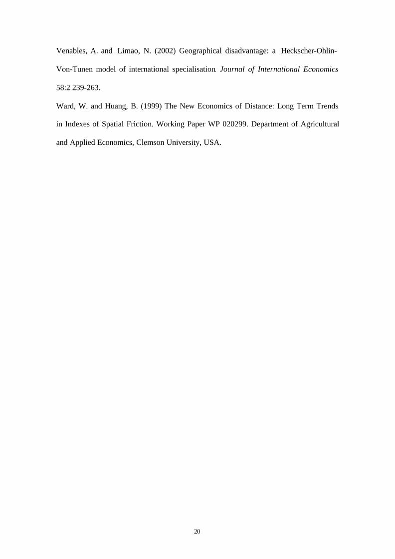
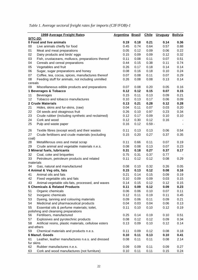
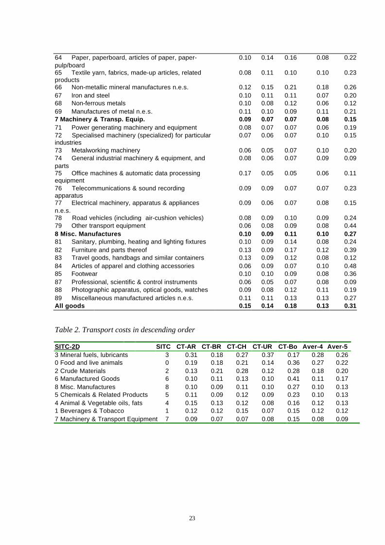
Table 1 shows the average sectoral (unweighted) freight rates for imports at 2 digits

SITC and Table 2 presents the average transport costs for sectors at 1 digit level in

descending order. In Table 3 a comparison is made for Argentinean imports of trade-

weighted and unweighted freight rates. The rates suggest that destinations with the

lowest ad-valorem transport costs have the largest share of trade, since the unweighted

freight rate is almost always higher than the corresponding trade-weighted freight rate.

The same occurs for the other five importers.

Our data correspond to those of Hummels (1999) in that they show how transport costs

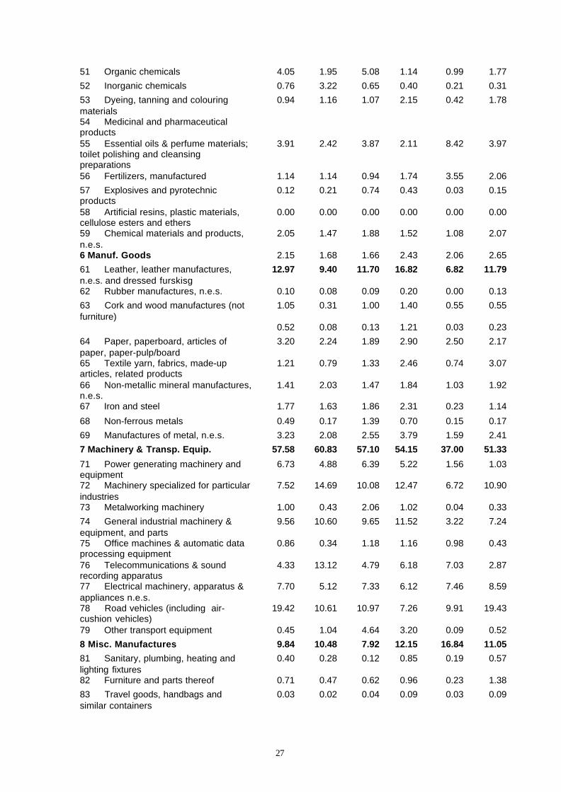
might play a relevant role in allocating trade over partner countries. Table 4 shows the

percentage shares of sectoral imports with respect to total imports from the EU. Imports

are concentrated in the manufacturing categories (sectors 5, 6, 7 and 8 at 1-digit level

SITC). Machinery & Transport Equipment show the highest share (higher that 50%) of

total imports from the EU and Chemicals & Related products present a share close to

15%. Table 5 reports the 15 products at 2 digit level with a highest share in total imports

from the EU, the first positions are for products of group 7 (machinery and transport

equipment).

Table 6 classifies imports by transportation mode. We observe that more than 50% of

total imports are transported by sea. For Brazil and Chile the percentages are close to

10

70%. Accordingly, we believe that port efficiency may play an important role in

fostering trade.

4. What factors explain transport costs?

A general formulation of transport costs for commodity k shipped between countries i

and j, in a given period of time, can be written as:

TCijk = F(Xi, Xj, vij, xijk, µk, ηij ) (1)

where Xi and Xj are country specific characteristics, vij is a vector of characteristics

relating the journey between i and j, xijk a vector of characteristics depending on the

country of origin and destination and the type of product (k), µk is a product specific

effect that captures differences in transport demand elasticity across goods and ηij

represents unobservable variables.

Among the country characteristics, Xi and Xj, we incorporate geographical and

infrastructure measures. Typically, dummy variables are used to control for a country

that is landlocked or an island. The infrastructure measure used is constructed as an

index with larger values of the index meaning a better infrastructure. In the vector of

characteristics, vij, distance between trading countries, volume of imports that goes

trough a particular route, and dummy variables for common language and common

border7, are usually considered. Among the characteristics depending also on the type of

product, xijk, we focus on the weight value for product k transported from country i to

country j. Product specific dummy variables are also modelled to account for µk.

Assuming a multiplicative form, a transport cost function can be written as:

1 2 33 51 2 4 i j ij kLand Land Langijk ijk ij ij i jTC W D Q Inf Inf eβ β β µα αα α α + + += (2)

7 The common border variable is not modelled since in the mutual trade UE-LA countries do not shareborders. The same applies for the island dummy.

11

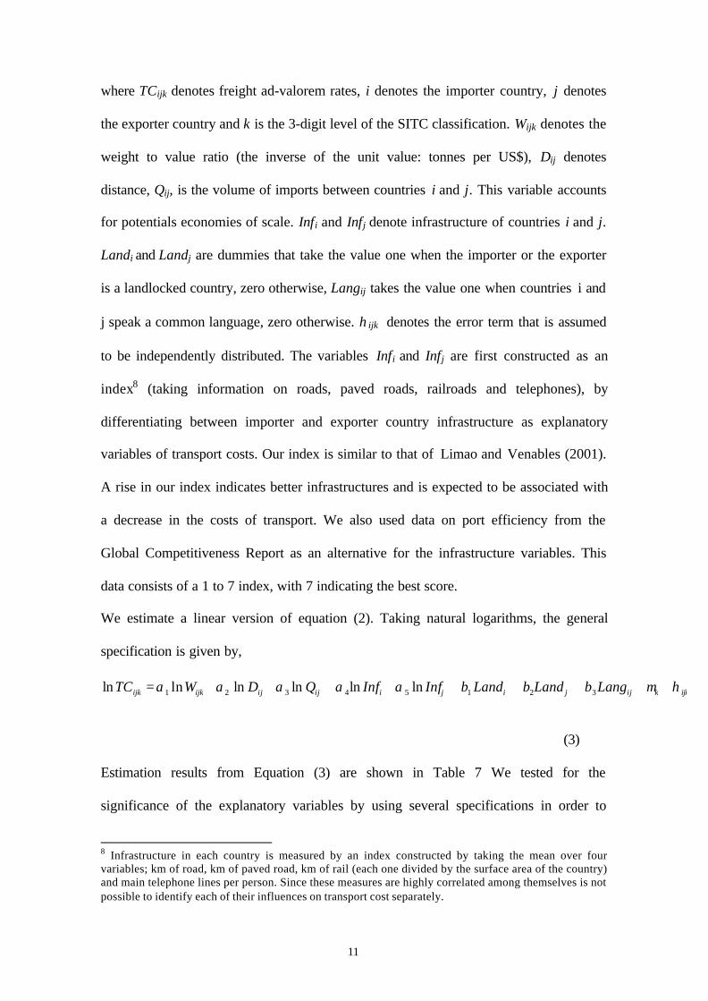
where TCijk denotes freight ad-valorem rates, i denotes the importer country, j denotes

the exporter country and k is the 3-digit level of the SITC classification. Wijk denotes the

weight to value ratio (the inverse of the unit value: tonnes per US$), Dij denotes

distance, Qij, is the volume of imports between countries i and j. This variable accounts

for potentials economies of scale. Infi and Infj denote infrastructure of countries i and j.

Landi and Landj are dummies that take the value one when the importer or the exporter

is a landlocked country, zero otherwise, Langij takes the value one when countries i and

j speak a common language, zero otherwise. ηijk denotes the error term that is assumed

to be independently distributed. The variables Infi and Infj are first constructed as an

index8 (taking information on roads, paved roads, railroads and telephones), by

differentiating between importer and exporter country infrastructure as explanatory

variables of transport costs. Our index is similar to that of Limao and Venables (2001).

A rise in our index indicates better infrastructures and is expected to be associated with

a decrease in the costs of transport. We also used data on port efficiency from the

Global Competitiveness Report as an alternative for the infrastructure variables. This

data consists of a 1 to 7 index, with 7 indicating the best score.

We estimate a linear version of equation (2). Taking natural logarithms, the general

specification is given by,

1 2 3 4 5 1 2 3ln ln ln ln ln lnijk ijk ij ij i j i j ij k ijkTC W D Q Inf Inf Land Land Langα α α α α β β β µ η= + + + + + + + + +

(3)

Estimation results from Equation (3) are shown in Table 7 We tested for the

significance of the explanatory variables by using several specifications in order to

8 Infrastructure in each country is measured by an index constructed by taking the mean over fourvariables; km of road, km of paved road, km of rail (each one divided by the surface area of the country)and main telephone lines per person. Since these measures are highly correlated among themselves is notpossible to identify each of their influences on transport cost separately.

12

compare our results with those obtained previously in the literature. In Model 1, we

estimated a pooled regression with only distance and weight variables. We include

importer country dummies to compare our results with those obtained by Hummels

(1999). The distance coefficient has the expected positive sign showing that a 10%

increase in distance increases transport costs by 5.3%. Our estimated distance elasticity

is higher than that found in other studies, even when we use commodity specific

distance coefficients (0.68 in Model 2). Using a very similar specification, Hummels

(1999) found commodity specific distance coefficients clustered in the 0.2 to 0.3 range.

Similarly, Micco and Pérez (2001) obtained a distance coefficient close to 0.2 in their

transport cost equation. However, when distance specific coefficients and sectoral

dummies are specified in the model, the significance level and the sign of the distance

coefficient varies greatly (Model 3), but still the average coefficient is high (0.68). One

reason for this disparity in results may be that trade costs associated with Latin

American imports are higher than trade costs associated with USA imports.

In Model 4 a Landi and Langij were added to the basic specification. Since in our sample

of exporters we do not have any landlocked country, Landj cannot be included. Both

estimated coefficients are significant at conventional levels. They indicate that when the

importer is a landlocked country transport costs are a 61% [exp(0.48)-1]*100 higher

than when it is a coastal country. A common language reduces transport costs in a 5%

[exp(-0.05)-1]*100. Infrastructure variables were added In Model 5. The importer

infrastructure variable shows a statistically significant coefficient with the expected

negative sign. We can interpret the importer infrastructure variable as a proxy for port

infrastructure when the transport is by ship. The estimated coefficient indicates that

poor infrastructure notably increases transport costs for importers: a 1% increase in

infrastructure reduces transport costs by 0.29%. On the other hand, the coefficient on

13

Infj shows that the reduction in transport costs induced from an improvement of 1% in

the exporter infrastructure is only of 0.05%. We show that the distance coefficient

remains statistically significant but with a significantly lower magnitude (0.14) when

infrastructure variables were added. When port efficiency is replaced by the

infrastructure index, Infi still shows a negative and significant coefficient, slightly

higher in magnitude (-0.37), showing that an increase in port efficiency reduces

transport costs for LA countries. However the coefficient on Infj is non significant and

positive signed, may be because European ports have already reached a considerable

level of port efficiency, compared to LA ports.

Models 6 and 7 show that economies of scale are also a relevant variable explaining the

variation of transport costs. Model 6 presents the results obtained when import volumes

are considered as an exogenous variable. The estimated elasticity is -0.10 and we

observed that the distance coefficient loses significance and the infrastructure

elasticities are lower than before but still significant. Since this model may suffer from

endogeneity problems -lower transport costs induce more trade- we performed a new

estimation considering the import volume as endogenous (Model 7). The estimated

elasticity for Qij is only slightly reduced in magnitude (-0.06) and the rest of estimated

parameters are very similar. This confirms the importance of economies of scale. Our

estimated elasticity is only slightly higher than that reported by Micco and Pérez

(2001)9.

5. Trade and transport costs

In order to assess the relative importance of transport costs on trade we need an

appropriate theoretical framework. In recent years, the gravity model of trade has

9 Micco and Perez (2001) found that using instrumental variables the economy of scale variable remainednegative and highly significant, but the magnitude of the coefficient increased in absolute value (-0.042v/s -0.025).

14

become the workhorse of international trade. From the large empirical literature, it is

commonly accepted that gravity models explain well bilateral trade patterns.

According to the simplest gravity model of trade, the volume of imports (exports)

between pairs of countries, Mij, is a function of their incomes (GDPs), their

geographical distance and a set of dummies,

31 2 40ij i j ij ij ijM Y Y D A uββ β ββ= (4)

where Yi (Yj) indicates GDPs of the exporter (importer), Dij measures the distance

between the two countries’ capitals (or economic centres) and Aij represents any other

factors aiding or preventing trade between pairs of countries. uij is the error term.

Trade is expected to be positive related to economic mass and negative related to

distance. The majority of estimates of the gravity equation are based on a log-linear

transformation of equation (4),

0 1 2 3ln ln ln lnij i j ij h ijh ijh

M Y Y D P uβ β β β δ= + + + + +∑ (5)

where ln denotes variables in natural logs. ijhh

h P∑δ is a sum of preferential trade

dummy variables. Pijh takes the value one when a certain condition is satisfied e.g.

belonging to a trade bloc, zero otherwise. Usually models include dummy variables for

trading partners sharing a common language and common border as well as trading

blocs dummy variables evaluating the effects of preferential trading agreements. The

coefficients of all these trade variables (δh) are expected to be positive.

Theoretical support of the research in this field was originally very poor, but since the

second half of the 1970s several theoretical developments have appeared in support of

the gravity model. Although distance is included in all empirical gravity models, the

theoretical models relate trade to transport costs, for which distance is a proxy.

15

The relationship between trade cost and distance, already specified in equation (3)

above, indicates that the elasticity of trade cost with respect to distance is positive, so

α2>0.

Starting with a theoretical model that relates bilateral trade with income and transport

costs and then substituting equation (3) for transport cost, one gets an augmented

gravity equation relating trade to distance and other variables,

1 2 4ln ln ln lnijk k i j ijk ijX Y Y TCγ γ γ γ µ= + + + + (6)

where

1 2 3 4 5 1 2 3ln ln ln ln ln lnijk ijk ij i j i j i j ij k ijkTC W D Q Inf Inf Land Land Langα α α α α β β β µ η= + + + + + + + + +

(7)

The model is estimated for bilateral exports from twelve EU countries to five Latin

American importers with data for 1998 disaggregated at 3 digits level (SITC). We

performed OLS estimation on the double log specification as given by equations (6) and

(7).

In the standard model (Equation 5 without dummies) α3 is a 'gross' distance elasticity of

trade, while in the models augmented with infrastructure or/and dummies and once

controlled for the composition of trade (sectoral dummies), the distance elasticity is a

'residual'.

Table 8 shows our results for aggregate trade flows. Model 1 presents the OLS results

for the baseline case, which excludes infrastructure variables and dummies and γk=γ.

(there are no sectoral effects). The standard regressors are income and distance

variables. The coefficients on the income variables show the expected positive sing. The

income elasticity is lower for the importer income (0.68). The exporter income elasticity

16

(1.06) indicates a high sensitivity of LA imports to the EU economic cycle. Both are

significant at 1% level. In Model 2, sectoral dummies at 2 digit level are added to the

list of explanatory variables. Their inclusion considerably improves the fit of the

regression and the distance coefficient increases slightly in magnitude. In Model 3 we

add the landlocked and language dummy variables, the estimated coefficients indicate

that a landlocked country trades a 56% less than a non-landlocked country and sharing a

language increases trade in a 289%. The inclusion of these dummies considerable

reduces the distance coefficient (-0.24). Infrastructure variables are added in Models 4

and 5. In model 4 we used the infrastructure index similar to Limao&Venables. The

importer infrastructure has a positive and significant coefficient, thus showing that an

improvement in the infrastructure in LA countries will foster trade, whereas the exporter

infrastructure coefficient is not significant. We can observe how the distance coefficient

is still significant and it shows the correct sign but a different magnitude (-0.77). In

Model 5 port efficiency is used as a proxy for port infrastructure. The fit of the equation

is slightly better that in Model 4, the estimated coefficient for Liporti indicates that

higher levels of efficiency in LA ports leads to an increase in imports. However, Liportj

has a negative coefficient, which is significant at conventional levels. Additionally, the

distance coefficient has an implausible large coefficient which is not significant.

Model 6 adds language to the list of explanatory variables, the estimated coefficient

indicates that sharing a language increases mutual trade and therefore cultural

similarities play an important role in international trade. In Model 7 transport cost is

directly introduced n the trade equation. First this variable is considered as exogenously

determined and finally, the mutual relationship between trade and transport cost is

modelled. The results point towards the importance of this mutual relationship.

17

6. Concluding comments

The objective of this paper was to investigate the determinants of transport costs and the

nature of the relationship between trade and transport costs. We estimated a transport

costs equation using data on transportation costs for five Latin-American countries. We

also studied the relationship between transport costs and trade and we estimated an

export demand model.

We considered as a source of variation in trade costs composition effects, as well as unit

values, distance and infrastructure variables. The results from our first estimation show

that higher distance and poor partner infrastructure notably increase transport costs.

Inclusion of infrastructure measures improves the fit of the regression, corroborating the

importance of infrastructure in determining transport costs. The distance coefficient

remains significant and does not always decreases in magnitude when we add

infrastructure. Economies of scale proxied by trade volume are also a relevant variable

explaining the variation of transport costs.

The results from our second estimation show that importer and exporter income

variables, as expected, have a positive influence in bilateral trade flows. Importer

income elasticity is lower than exporter income elasticity. Being landlocked

significantly deters trade, cultural similarities, as sharing a language, foster trade.

Finally, a trade elasticity with respect to transport cost of 2.29 was estimated when we

considered the mutual relationship between trade and transport costs.

Future estimations for more countries and years, will be of interest so as to find out

more about the effects of transportation costs on trade flows under diverse conditions of

international transport.

18

References

Coe, D. T., Subramanian, A. and Tamirisa, N. T. (2002) The Missing Globalization

Puzzle, International Monetary Fund Working Paper (WP/02/171).

Deardorff, A. (2001) Local Comparative Advantage, Trade Costs and the Pattern of

Trade, processed. University of Michigan.

Baier, S. L. and Bergstrand, J. H. (2001) The Growth of World Trade: Tariffs, Transport

Costs, and Income Similarity. Journal of International Economics 53: 1-27.

Dixit, A.and Stiglitz, J. E. (1977) Monopolistic Competition and Optimum Product

Diversity, American Economic Review 67: 297-308.

Donald, D. and Weinstein, D. (1996) Does Economic Geography Matters for

International Specialisation?. National Bureau of Economic Research Working Paper

5706.

Fink, C., Mattoo, A. Neagu, I. C. (2000) Trade In International Maritime Service: How

Much Does Policy Matter?. Washington DC, United States, World Bank.

Henderson, J. V., Shalizi, Z., Venables, A. J. (2001) Geography and Development.

Journal of Economic Geography, 1:81-106.

Hoffmann, J. and Kumar, S. (2002) Globalization - The Maritime Nexus. In Handbook

of Maritime Economics, LLP, London. Forthcoming fall 2002.

Hummels, D. (1999) Towards A Geography of Trade Costs. University of Chicago.

Mimeographed document.

Hummels, D. (2001) Have International Transportation Costs Declined?. Journal of

International Economics 54 (1): 75-96.

Humels, D., Ishii, J., Yi, K-M. (2001) The Nature and Growth of Vertical Specialisation

in World Trade. Journal of International Economics (forthcoming).

19

Krugman, P. (1991) Increasing Returns and Economic Geography. Journal of Political

Economy 99 (3): 483-499.

Limao, N., Venables, A. J. (2001) Infrastructure, Geographical Disadvantage and

Transport Costs. World Bank Economic Review, 15 (3): 451-479.

Markusen, J., Venables, A. J. (1996) The Theory of Endowment, Intra-Industry and

Multinational Trade. National Bureau of Economic Research Working Paper 5529.

Martínez-Zarzoso, I., García-Menendez, L. and Suárez-Burguet, C. (2003) The Impact

of Transport Cost on International Trade: The Case of Spanish Ceramic Exports.

Maritime Economics & Logistics (forthcoming).

Micco, A., Pérez, N. (2001) Maritime Transport Costs and Port Efficiency. Inter-

American Development Bank, Research Working Paper.

Oguledo, V.I., Macphee, C.R. (1994) Gravity models: a reformulation and an

application to discriminatory trade arrangements. Applied Economics, 26: 107-120.

Radelet, S., Sachs, J. (1998) Shipping Costs, Manufactured Exports and Economic

Growth. Harvard University, Harvard Institute for International Development.

Mimeographed document.

Rauch, J. E. (1999) Networks Versus Markets in International Trade. Journal of

International Economics, 48: 7:35.

Sánchez, R. J., Hoffmann, J., Micco, A., Pizzolitto G. and Sgut, M. (2002)

Port Efficiency and International Trade, Conference proceedings, IAME annual meeting

and conference, Panama, November (forthcoming).

Venables, A. (2001) Geography and International Inequalities: The Impact of New

Technologies. Journal of Industry, Competition and Trade, 1:2 135-159.

20

Venables, A. and Limao, N. (2002) Geographical disadvantage: a Heckscher-Ohlin-

Von-Tunen model of international specialisation. Journal of International Economics

58:2 239-263.

Ward, W. and Huang, B. (1999) The New Economics of Distance: Long Term Trends

in Indexes of Spatial Friction. Working Paper WP 020299. Department of Agricultural

and Applied Economics, Clemson University, USA.

21

Figure 1. Freight rates across sectors (1-digit level) and across importers (imports from

the EU in 1998)

0,00

0,05

0 , 1 0

0 , 1 5

0,20

0,25

0,30

0,35

0,40

0,45

0 Food and live

animals

1 Beberages &

Tobacco

2 Crude Mater ia ls 3 M inera l fue ls ,

lubr icants

4 Animal & Veg oils,

f a t s

5 Chemicals &

Related Prod.

6 Manuf. Goods 7 Machinery &

Transp. Equip.

8 Misc .

Manufactures

CT-AR

CT-BR

CT-CH

CT-UR

CT-Bo

22

Table 1. Average sectoral freight rates for imports (CIF/FOB)-1

1998SITC-2D:

Average Freight Rates Argentina Brasil Chile Uruguay Bolivia

0 Food and live animals 0.19 0.18 0.21 0.14 0.3600 Live animals chiefly for food 0.45 0.74 0.64 0.57 0.8801 Meat and meat preparations 0.05 0.12 0.09 0.06 0.2202 Dairy products and birds' eggs 0.15 0.09 0.09 0.12 0.3203 Fish, crustaceans, molluscs, preparations thereof 0.11 0.08 0.11 0.07 0.5104 Cereals and cereal preparations 0.44 0.15 0.38 0.11 0.7405 Vegetables and fruit 0.26 0.17 0.18 0.14 0.1406 Sugar, sugar preparations and honey 0.08 0.16 0.18 0.10 0.2407 Coffee, tea, cocoa, spices, manufactures thereof 0.07 0.08 0.11 0.07 0.2908 Feeding stuff for animals, not including unmilledcereals

0.26 0.08 0.08 0.13 0.14

09 Miscellaneous edible products and preparations 0.07 0.08 0.20 0.05 0.161 Beverages & Tobacco 0.12 0.12 0.15 0.07 0.1511 Beverages 0.15 0.11 0.13 0.09 0.2112 Tobacco and tobacco manufactures 0.10 0.13 0.17 0.06 0.092 Crude Materials 0.13 0.21 0.28 0.12 0.2821 Hides, skins and fur-skins, (raw) 0.04 0.11 0.07 0.03 0.2022 Oil seeds and oleaginous fruit 0.26 0.10 0.97 0.23 0.3423 Crude rubber (including synthetic and reclaimed) 0.12 0.17 0.09 0.10 0.1024 Cork and wood 0.12 0.30 0.12 0.16 -25 Pulp and waste paper 0.16 0.12 0.59 - -

26 Textile fibres (except wool) and their wastes 0.11 0.13 0.13 0.06 0.5427 Crude fertilisers and crude materials (excludingcoal)

0.15 0.20 0.27 0.37 0.35

28 Metalliferous ores and metal scrap 0.11 0.66 0.11 0.07 0.1929 Crude animal and vegetable materials n.e.s. 0.08 0.08 0.13 0.07 0.233 Mineral fuels, lubricants 0.31 0.18 0.27 0.37 0.1732 Coal, coke and briquettes 0.75 0.31 0.37 0.77 -33 Petroleum, petroleum products and relatedmaterials

0.11 0.12 0.12 0.08 0.29

34 Gas, natural and manufactured 0.08 0.10 0.32 0.26 0.054 Animal & Veg oils, fats 0.15 0.13 0.12 0.08 0.1641 Animal oils and fats 0.21 0.14 0.15 0.09 0.1942 Fixed vegetable oils and fats 0.10 0.09 0.09 0.03 0.1543 Animal-vegetable oils-fats, processed, and waxes 0.14 0.15 0.12 0.12 0.155 Chemicals & Related Products 0.11 0.09 0.12 0.09 0.2351 Organic chemicals 0.06 0.06 0.10 0.07 0.1152 Inorganic chemicals 0.12 0.11 0.19 0.11 0.4553 Dyeing, tanning and colouring materials 0.09 0.06 0.11 0.09 0.2154 Medicinal and pharmaceutical products 0.04 0.03 0.04 0.06 0.1355 Essential oils & perfume materials; toilet,polishing and cleansing preparations

0.11 0.10 0.10 0.12 0.19

56 Fertilisers, manufactured 0.25 0.14 0.19 0.10 0.5157 Explosives and pyrotechnic products 0.08 0.12 0.12 0.09 0.3458 Artificial resins, plastic materials, cellulose estersand ethers

0.13 0.09 0.10 0.12 0.14

59 Chemical materials and products n.e.s. 0.11 0.09 0.12 0.08 0.186 Manuf. Goods 0.10 0.11 0.13 0.10 0.4161 Leather, leather manufactures n.e.s. and dressedfur skins

0.08 0.11 0.11 0.08 2.14

62 Rubber manufactures n.e.s. 0.09 0.09 0.11 0.09 0.2763 Cork and wood manufactures (not furniture) 0.10 0.11 0.11 0.15 0.24

23

64 Paper, paperboard, articles of paper, paper-pulp/board

0.10 0.14 0.16 0.08 0.22

65 Textile yarn, fabrics, made-up articles, relatedproducts

0.08 0.11 0.10 0.10 0.23

66 Non-metallic mineral manufactures n.e.s. 0.12 0.15 0.21 0.18 0.2667 Iron and steel 0.10 0.11 0.11 0.07 0.2068 Non-ferrous metals 0.10 0.08 0.12 0.06 0.1269 Manufactures of metal n.e.s. 0.11 0.10 0.09 0.11 0.217 Machinery & Transp. Equip. 0.09 0.07 0.07 0.08 0.1571 Power generating machinery and equipment 0.08 0.07 0.07 0.06 0.1972 Specialised machinery (specialized) for particularindustries

0.07 0.06 0.07 0.10 0.15

73 Metalworking machinery 0.06 0.05 0.07 0.10 0.2074 General industrial machinery & equipment, andparts

0.08 0.06 0.07 0.09 0.09

75 Office machines & automatic data processingequipment

0.17 0.05 0.05 0.06 0.11

76 Telecommunications & sound recordingapparatus

0.09 0.09 0.07 0.07 0.23

77 Electrical machinery, apparatus & appliancesn.e.s.

0.09 0.06 0.07 0.08 0.15

78 Road vehicles (including air-cushion vehicles) 0.08 0.09 0.10 0.09 0.2479 Other transport equipment 0.06 0.08 0.09 0.08 0.448 Misc. Manufactures 0.10 0.09 0.11 0.10 0.2781 Sanitary, plumbing, heating and lighting fixtures 0.10 0.09 0.14 0.08 0.2482 Furniture and parts thereof 0.13 0.09 0.17 0.12 0.3983 Travel goods, handbags and similar containers 0.13 0.09 0.12 0.08 0.1284 Articles of apparel and clothing accessories 0.06 0.09 0.07 0.10 0.4885 Footwear 0.10 0.10 0.09 0.08 0.3687 Professional, scientific & control instruments 0.06 0.05 0.07 0.08 0.0988 Photographic apparatus, optical goods, watches 0.09 0.08 0.12 0.11 0.1989 Miscellaneous manufactured articles n.e.s. 0.11 0.11 0.13 0.13 0.27All goods 0.15 0.14 0.18 0.13 0.31

Table 2. Transport costs in descending order

SITC-2D SITC CT-AR CT-BR CT-CH CT-UR CT-Bo Aver-4 Aver-53 Mineral fuels, lubricants 3 0.31 0.18 0.27 0.37 0.17 0.28 0.260 Food and live animals 0 0.19 0.18 0.21 0.14 0.36 0.27 0.222 Crude Materials 2 0.13 0.21 0.28 0.12 0.28 0.18 0.206 Manufactured Goods 6 0.10 0.11 0.13 0.10 0.41 0.11 0.178 Misc. Manufactures 8 0.10 0.09 0.11 0.10 0.27 0.10 0.135 Chemicals & Related Products 5 0.11 0.09 0.12 0.09 0.23 0.10 0.134 Animal & Vegetable oils, fats 4 0.15 0.13 0.12 0.08 0.16 0.12 0.131 Beverages & Tobacco 1 0.12 0.12 0.15 0.07 0.15 0.12 0.127 Machinery & Transport Equipment 7 0.09 0.07 0.07 0.08 0.15 0.08 0.09

24

Table 3. Comparison of unweighted and weighted sectoral freight rates for Argentinean

imports (CIF/FOB)-1

1998SITC-2D:

Average Freight Rates Unweithed Weighted

0 Food and live animals 0.19 0,1000 Live animals chiefly for food 0.45 0,2701 Meat and meat preparations 0.05 0,0402 Dairy products and birds' eggs 0.15 0,0903 Fish, crustaceans, molluscs, preparations thereof 0.11 0,0604 Cereals and cereal preparations 0.44 0,1405 Vegetables and fruit 0.26 0,1106 Sugar, sugar preparations and honey 0.08 0,0607 Coffee, tea, cocoa, spices, manufactures thereof 0.07 0,0708 Feeding stuff for animals, not including unmilled cereals 0.26 0,0709 Miscellaneous edible products and preparations 0.07 0,071 Beverages & Tobacco 0.12 0,0611 Beverages 0.15 0,0512 Tobacco and tobacco manufactures 0.10 0,062 Crude Materials 0.13 0,1221 Hides, skins and fur-skins, raw 0.04 0,0422 Oil seeds and oleaginous fruit 0.26 0,1423 Crude rubber (including synthetic and reclaimed) 0.12 0,0924 Cork and wood 0.12 0,1325 Pulp and waste paper 0.16 0,1726 Textile fibres (except wool tops) and their wastes 0.11 0,0827 Crude fertilizers and crude materials (excluding coal) 0.15 0,2728 Metalliferous ores and metal scrap 0.11 0,0829 Crude animal and vegetable materials, n.e.s. 0.08 0,073 Mineral fuels, lubricants 0.31 0,3032 Coal, coke and briquettes 0.75 0,7033 Petroleum, petroleum products and related materials 0.11 0,1334 Gas, natural and manufactured 0.08 0,084 Animal & Veg oils, fats 0.15 0,1141 Animal oils and fats 0.21 0,1942 Fixed vegetable oils and fats 0.10 0,0543 Animal-vegetable oils-fats, processed, and waxes 0.14 0,105 Chemicals & Related Products 0.11 0,0851 Organic chemicals 0.06 0,0452 Inorganic chemicals 0.12 0,1253 Dyeing, tanning and colouring materials 0.09 0,0654 Medicinal and pharmaceutical products 0.04 0,0355 Essential oils & perfume materials; toilet polishing andcleansing preparations

0.11 0,06

56 Fertilizers, manufactured 0.25 0,2257 Explosives and pyrotechnic products 0.08 0,0758 Artificial resins, plastic materials, cellulose esters andethers

0.13 0,07

59 Chemical materials and products, n.e.s. 0.11 0,056 Manuf. Goods 0.10 0,0861 Leather, leather manufactures, n.e.s. and dressedfurskisg

0.08 0,05

62 Rubber manufactures, n.e.s. 0.09 0,0763 Cork and wood manufactures (not furniture) 0.10 0,06

25

64 Paper, paperboard, articles of paper, paper-pulp/board 0.10 0,0965 Textile yarn, fabrics, made-up articles, related products 0.08 0,0766 Non-metallic mineral manufactures, n.e.s. 0.12 0,1167 Iron and steel 0.10 0,0868 Non-ferrous metals 0.10 0,0669 Manufactures of metal, n.e.s. 0.11 0,137 Machinery & Transp. Equip. 0.09 0,0571 Power generating machinery and equipment 0.08 0,0572 Machinery specialized for particular industries 0.07 0,0473 Metalworking machinery 0.06 0,0474 General industrial machinery & equipment, and parts 0.08 0,0575 Office machines & automatic data processingequipment

0.17 0,04

76 Telecommunications & sound recording apparatus 0.09 0,0277 Electrical machinery, apparatus & appliances n.e.s. 0.09 0,0678 Road vehicles (including air-cushion vehicles) 0.08 0,0679 Other transport equipment 0.06 0,048 Misc. Manufactures 0.10 0,0781 Sanitary, plumbing, heating and lighting fixtures 0.10 0,0882 Furniture and parts thereof 0.13 0,1183 Travel goods, handbags and similar containers 0.13 0,0984 Articles of apparel and clothing accessories 0.06 0,0385 Footwear 0.10 0,1087 Professional, scientific & controlling instruments 0.06 0,0488 Photographic apparatus, optical goods, watches 0.09 0,0489 Miscellaneous manufactured articles, n.e.s. 0.11 0,07All goods 0.15 0.09

26

Table 4. Percentage shares of sectoral imports with respect to total imports from theEU

1998 %sharesSITC-2D:

M from the EU-15

Argent. Bolibia Brazil Chile Paraguay Uruguay

0 Food and live animals 2.04 3.26 3.53 2.11 1.44 3.13

00 Live animals chiefly for food 0.03 0.07 0.04 0.06 0.00 0.03

01 Meat and meat preparations 0.47 0.02 0.04 0.07 0.02 0.08

02 Dairy products and birds' eggs 0.17 2.06 0.44 0.49 0.05 0.12

03 Fish, crustaceans, molluscs,preparations thereof

0.14 0.09 1.11 0.09 0.08 0.46

04 Cereals and cereal preparations 0.20 0.42 0.65 0.17 0.23 0.27

05 Vegetables and fruit 0.38 0.06 0.71 0.24 0.48 1.14

06 Sugar, sugar preparations andhoney

0.08 0.11 0.09 0.07 0.11 0.15

07 Coffee, tea, cocoa, spices,manufactures thereof

0.21 0.13 0.08 0.23 0.19 0.38

08 Feeding stuff for animals, notincluding unmilled cereals

0.15 0.16 0.14 0.21 0.16 0.12

09 Miscellaneous edible products andpreparations

0.23 0.14 0.24 0.48 0.13 0.39

1 Beverages & Tobacco 0.58 1.33 0.81 0.82 19.97 5.75

11 Beverages 0.56 1.30 0.70 0.80 19.71 5.15

12 Tobacco and tobaccomanufactures

0.02 0.02 0.11 0.03 0.26 0.59

2 Crude Materials 0.64 1.03 0.77 1.04 0.20 1.00

21 Hides, skins and fur-skins, raw 0.04 0.00 0.02 0.00 0.00 0.00

22 Oil seeds and oleaginous fruit 0.00 0.00 0.00 0.00 0.00 0.00

23 Crude rubber (including syntheticand reclaimed)

0.05 0.03 0.05 0.04 0.00 0.32

24 Cork and wood 0.05 0.00 0.04 0.03 0.00 0.01

25 Pulp and waste paper 0.02 0.00 0.01 0.01 0.01 0.00

26 Textile fibres (except wool tops)and their wastes

0.07 0.83 0.09 0.51 0.16 0.11

27 Crude fertilizers and crudematerials (excluding coal)

0.09 0.03 0.14 0.07 0.01 0.21

28 Metalliferous ores and metal scrap 0.01 0.01 0.09 0.00 0.00 0.00

29 Crude animal and vegetablematerials, n.e.s.

0.31 0.14 0.33 0.37 0.02 0.34

3 Mineral fuels, lubricants 1.07 0.16 1.85 0.69 0.83 0.99

32 Coal, coke and briquettes 0.00 0.00 0.00 0.01 0.00 0.00

33 Petroleum, petroleum products andrelated materials

1.07 0.16 1.70 0.64 0.83 0.98

34 Gas, natural and manufactured 0.00 0.00 0.15 0.05 0.00 0.00

4 Animal & Veg. oils, fats 0.16 0.27 0.42 0.30 0.14 0.20

41 Animal oils and fats 0.02 0.03 0.01 0.01 0.00 0.02

42 Fixed vegetable oils and fats 0.09 0.22 0.37 0.08 0.10 0.17

43 Animal-vegetable oils-fats,processed, and waxes

0.05 0.01 0.04 0.21 0.04 0.01

5 Chemicals & Related Products 15.12 13.25 15.90 11.92 16.76 14.76

27

51 Organic chemicals 4.05 1.95 5.08 1.14 0.99 1.77

52 Inorganic chemicals 0.76 3.22 0.65 0.40 0.21 0.31

53 Dyeing, tanning and colouringmaterials

0.94 1.16 1.07 2.15 0.42 1.78

54 Medicinal and pharmaceuticalproducts55 Essential oils & perfume materials;toilet polishing and cleansingpreparations

3.91 2.42 3.87 2.11 8.42 3.97

56 Fertilizers, manufactured 1.14 1.14 0.94 1.74 3.55 2.06

57 Explosives and pyrotechnicproducts

0.12 0.21 0.74 0.43 0.03 0.15

58 Artificial resins, plastic materials,cellulose esters and ethers

0.00 0.00 0.00 0.00 0.00 0.00

59 Chemical materials and products,n.e.s.

2.05 1.47 1.88 1.52 1.08 2.07

6 Manuf. Goods 2.15 1.68 1.66 2.43 2.06 2.65

61 Leather, leather manufactures,n.e.s. and dressed furskisg

12.97 9.40 11.70 16.82 6.82 11.79

62 Rubber manufactures, n.e.s. 0.10 0.08 0.09 0.20 0.00 0.13

63 Cork and wood manufactures (notfurniture)

1.05 0.31 1.00 1.40 0.55 0.55

0.52 0.08 0.13 1.21 0.03 0.23

64 Paper, paperboard, articles ofpaper, paper-pulp/board

3.20 2.24 1.89 2.90 2.50 2.17

65 Textile yarn, fabrics, made-uparticles, related products

1.21 0.79 1.33 2.46 0.74 3.07

66 Non-metallic mineral manufactures,n.e.s.

1.41 2.03 1.47 1.84 1.03 1.92

67 Iron and steel 1.77 1.63 1.86 2.31 0.23 1.14

68 Non-ferrous metals 0.49 0.17 1.39 0.70 0.15 0.17

69 Manufactures of metal, n.e.s. 3.23 2.08 2.55 3.79 1.59 2.41

7 Machinery & Transp. Equip. 57.58 60.83 57.10 54.15 37.00 51.33

71 Power generating machinery andequipment

6.73 4.88 6.39 5.22 1.56 1.03

72 Machinery specialized for particularindustries

7.52 14.69 10.08 12.47 6.72 10.90

73 Metalworking machinery 1.00 0.43 2.06 1.02 0.04 0.33

74 General industrial machinery &equipment, and parts

9.56 10.60 9.65 11.52 3.22 7.24

75 Office machines & automatic dataprocessing equipment

0.86 0.34 1.18 1.16 0.98 0.43

76 Telecommunications & soundrecording apparatus

4.33 13.12 4.79 6.18 7.03 2.87

77 Electrical machinery, apparatus &appliances n.e.s.

7.70 5.12 7.33 6.12 7.46 8.59

78 Road vehicles (including air-cushion vehicles)

19.42 10.61 10.97 7.26 9.91 19.43

79 Other transport equipment 0.45 1.04 4.64 3.20 0.09 0.52

8 Misc. Manufactures 9.84 10.48 7.92 12.15 16.84 11.05

81 Sanitary, plumbing, heating andlighting fixtures

0.40 0.28 0.12 0.85 0.19 0.57

82 Furniture and parts thereof 0.71 0.47 0.62 0.96 0.23 1.38

83 Travel goods, handbags andsimilar containers

0.03 0.02 0.04 0.09 0.03 0.09

28

84 Articles of apparel and clothingaccessories

0.69 0.47 0.34 2.05 0.66 1.30

85 Footwear 0.04 0.10 0.03 0.77 0.10 0.17

87 Professional, scientific & controllinginstruments

2.51 2.34 3.14 2.47 3.93 1.85

88 Photographic apparatus, opticalgoods, watches

0.88 0.71 0.87 0.86 1.64 0.66

89 Miscellaneous manufacturedarticles, n.e.s.

4.58 6.10 2.78 4.11 10.06 5.03

All goods

Table 5. Main products imported from the EU1998 % Over total M from the EUSITC Argent. Bolibia Brazil Chile Paraguay Uruguay

78 19.42 10.61 10.97 7.26 9.91 19.43 74 9.56 10.60 9.65 11.52 3.22 7.24 77 7.70 5.12 7.33 6.12 7.46 8.59 72 7.52 14.69 10.08 12.47 6.72 10.90

71 6.73 4.88 6.39 5.22 1.56 1.03 89 4.58 6.10 2.78 4.11 10.06 5.03 76 4.33 13.12 4.79 6.18 7.03 2.87 51 4.05 1.95 5.08 1.14 0.99 1.77 54 3.91 2.42 3.87 2.11 8.42 3.97 69 3.23 2.08 2.55 3.79 1.59 2.41 64 3.20 2.24 1.89 2.90 2.50 2.17 87 2.51 2.34 3.14 2.47 3.93 1.85 59 2.15 1.68 1.66 2.43 2.06 2.65 58 2.05 1.47 1.88 1.52 1.08 2.07 67 1.77 1.63 1.86 2.31 0.23 1.14

% 82.72 80.91 73.90 71.54 66.76 73.11

Table 6. Imports by transportation mode

Country Air Road RailMaritime

(including river and lake)Others and not stated

Argentina 17.49% 22.34% 0.65% 56.57% 2.96%Bolivia 0.00% 0.00% 0.00% 0.00% 100.00%Brazil 24.31% 8.20% 0.21% 66.72% 0.56%Chile 17.02% 11.42% 0.09% 68.09% 3.38%Uruguay 12.47% 42.45% 0.10% 44.95% 0.03%

29

Table 7 Spatial structure of freight rates for five importers in 1998

Intercepts Constant Weight-value (kg/$) Distance toexporter

ImporterInfrastructure

ExporterInfrastructure

R2 obs

Model 1:Pooled regressionArgentina -5.42 0.243 (46.84) 0.535 (5.39) - - 0.312 7298Bolivia -4.86Brazil -5.34Chile -5.31Uruguay -5.39Model 2: Regression with sectoral dummiesArgentina -4.83 0.256 (34.37) 0.687(7.12) - - 0.383 7298Bolivia -4.69Brazil -4.25Chile -4.73Uruguay -4.78

Model 3: Regression with distance-specific coefficientsAverageCoefficient

Argentina -6.73 0.2561 (34.37) 0.6889 (7.12) - - 0.383 7298Bolivia -6.16Brazil -6.59Chile -6.63Uruguay -6.68

Model 4: Regression with sectoral and landlocked dummiesLandlocked Lang

-3.07 (-5.61)

0.256 (34.66) 0.501 (8.89) 0.48 (19.61) -0.05 (-2.57) 0.3860 7313

Model 5: Regression with sectoral dummies and infrastructure variablesLvinfi Lvinfj

-0.64(-1.16)

0.2602(35.03)

0.14 (2.41)

-0.29(-17.1)

-0.05(-3.23)

0.369 7298

Liporti Liportj-3.08(-5.42)

0.264(25.47)

0.54(8.81)

-0.37(-14.37)

0.10(0.038)

0.360 7313

Model 6: Regression with sectoral dummies, infrastructure variables and exports volume Mvol Lvinfi Lvinfj -0.10 (-31.58)

3.21(6.07)

0.28(40.59)

-0.07(0.22)

-0.13(12.78)

-0.02(-1.64)

0.47 7328

Model 7: Regression with sectoral dummies, infrastructure variables and estimated exports volume Mvolf Lvinfi Lvinfj -0.06 (-11.83)

1.86(3.13)

0.27(26.82)

0.006(0.10)

-0.18(9.71)

-0.03(-2.10)

0.39 7328

Notes: Landlocked is a dummy that takes the value one when a country is landlocked, zero otherwise.Lang is a dummy that takes the value one when the trading countries speak a common language, zerootherwise. Lvinfi and Lvinfj are infrastructure indices of countries i and j. Liporti and Liportj are portinfrastructure measures for countries i and j. Mvol denotes import volume traded between countries i andj and Mvolf are estimated imports obtained from Model ... in Table 8.

30

Table 8 Aggregated estimates of Import DemandConstant Importer

GDPExporter

GDPDistance

toexporter

Landlocked

Lang ImporterInfrastr.

ExporterInfrastr.

Adj.R2

Model 1: Pooled regression

-37.83(0.68)

0.68(30.17)

1.06(31.85)

-0.53(-2.03)

- - - 0.207

Model 2: Regression with sectoral dummies

-40.57(-14.57)

0.69(32.47)

1.13(35.10)

-0.70 (-2.89)

- - - 0.344

Model 3 Regression with sectoral, landlocked and language dummies

-43.19 (-12.11)

0.618(20.24)

1.14(35.13)

-0.24(-0.83)

-0.83(-9.18)

1.36(14.3)

- 0.368

Model 4: Regression with sectoral dummies and infrastructure variablesLvinfi Lvinfj

-38.03 (-13.56)

0.64(28.06)

1.14(33.59)

-0.77(-3.15)

- - 0.28(3.96)

-0.10 (-1.52)

0.345

Model 5: Regression with sectoral dummies and port efficiency Liporti Liportj

-4.66 (-0.98)

0.28(6.15)

1.07(33.26)

-3.48(-0.33)

- 2.31 (10.78)

-0.44 (-2.12)

0.359

Model 6: Regression with sectoral and language dummies and port efficiency Lang Liporti Liportj

-34.92 (-6.31)

0.53(10.34)

1.12(5.23)

-0.90 (-1.86)

- 1.19 (11.51)

1.22 (5.23)

-0.59(-2.79)

0.370

Model 7: Regression with sectoral and language dummies, infrastructure and transport costsLang Lvinfi Lvinfj LTC

-34.20 0.71 0.99 - 0.97 0.27 -0.10 -0.79 0.47(-35.16) (42.86) (38.72) - (13.86) (4.95) (-1.06) (-20.8)

Lang Lvinfi Lvinfj LTCF-27.66 0.53 0.85 - 1.03 - - -2.29 0.54(-31.23) (34.31) (38.23) - (9.72) - (-43.3)

Notes: Landlocked is a dummy that takes the value one when a country is landlocked, zero otherwise.Lang is a dummy that takes the value one when the trading countries speak a common language, zerootherwise. Lvinfi and Lvinfj are infrastructure indices of countries i and j. Liporti and Liportj are portinfrastructure measures for countries i and j. LTC denotes freight rates and LTCF are estimated transportcosts obtained from Model 6 in Table 7.