Transparencies for the course TDDA41 Logic Programming ...

Transparencies for the course TDDA41 Logic

Programming, given at the Department of

Computer and Information Science, Linkoping

University, Sweden.

c©1998-2006, Ulf Nilsson ([email protected]).

Printout: November 25, 2006

Introduction: Overview

• Goals of the course.

• What is logic programming?

• Why logic programming?

1

Goals of the course

• Logic as a specification ANDprogramming language;

• Theoretical foundation of logicprogramming;

• Practice of Prolog and constraintprogramming;

• Relations to other areas:

– Databases

– Formal/natural languages

– Combinatorial problems

• To program DECLARATIVELY.

2

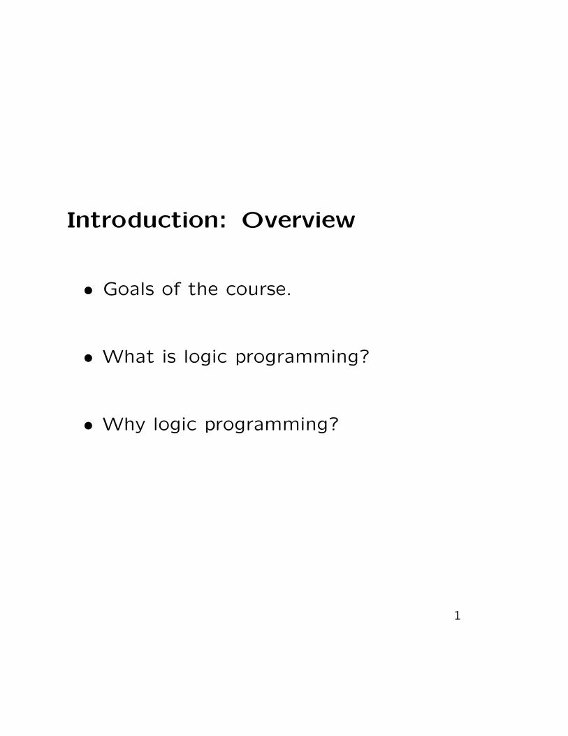
Declarative vs imperativelanguages

Imperative Declarative

Paradigm Describe HOWTO solve theproblem

DescribeWHAT theproblem is

Program A sequence ofcommands

A set of state-ments

Examples C, Fortran,Ada, Java

Prolog, PureLisp, Haskell,ML

Advantages Fast, special-ized programs

General,readable,correct(?)programs.

3

Declarative description A grandchild to x is

a child of one of x’s children.

Imperative description I To find a

grandchild of x, first find a child of x. Then

find a child of that child.

Imperative description II To find a

grandchild of x, first find a parent-child pair

and then check if the parent is a child of x.

Imperative description III To find a

grandchild of x, compute the factorial of 123,

then find a child of x. Then find a child of

that child.

4

Compare . . .

read(person);

for i := 1 to maxparent do

if parent[i;1] = person then

for j := 1 to maxparent do

if parent[j;1] = parent[i;2] then

write(parent[j;2]);

fi

od

fi

od

with . . .

gc(X,Z) :- c(X,Y), c(Y,Z).

5

Logic: Overview

• Syntax and semantics

• Vocabulary, terms and formulas

• Interpretations and models

• Logical consequence and equivalence

• Proofs/derivations

• Soundness and completeness

6

Predicate logic vocabulary

• Constants (17, george, tEX, . . .)

• Functors (cons/2,+/2, father/1, . . .)

• Predicate symbols

(member/2, </2, father/1, . . .)

• Variables (X, X11, , 123, T eX, . . .)

• Logical connectives (∧,∨,⊃,¬,↔)

• Quantifiers (∀,∃)

• Auxiliary symbols (., (, ), . . .)

7

Example

A = {volvo; owner/1; owns/2, happy/1}

8

Terms

Let A be a vocabulary.

The set of all terms over A is the least set

such that

• every constant in A is a term;

• every variable is a term;

• if f/n is a functor in A and t1, . . . , tn are

terms over A then f(t1, . . . , tn) is a term.

9

Ground terms

A term that contains no variables is called a

ground term.

10

(Well-formed) formulas


The set of all formulas over A is the least set

such that:

• if p/n is a predicate symbol in A and

t1, . . . , tn are terms, then p(t1, . . . , tn) is a

formula;

• if F and G are formulas, then

(F ∧G), (F ∨G), (F ⊃ G), (F ↔ G) and ¬F

are formulas;

• if F is a formula and X a variable, then

∀X F and ∃X F are formulas.

11

Atoms

A formula of the form p(t1, . . . , tn) is called an

atomic formula (atom).

Free occurrences of variables

An occurrence of X in a formula is said to be

free iff the occurrence does not follow

immediately after a quantifier, or in a formula

immediately after ∀X or ∃X.

Closed formulas

A formula that does not contain any free

occurrences of variables is said to be closed.

12

Universal closure

Assume that {X1, . . . , Xn} are the only free

occurrences of variables in a formula F . The

universal closure ∀F of F is the closed

formula ∀X1 . . . ∀Xn F .

The existential closure ∃F is defined similarly.

13

Interpretations


An interpretation � of A consists of (1) a

non-empty set D (often written |�|) of

objects (the domain of �) and (2) a function

that maps:

• every constant c in A on an element c� in

D;

• every functor f/n in A on a function

f� : Dn→ D;

• every predicate symbol p/n in A on a

relation p� ⊆ Dn.

14

Example

The vocabulary:


Consider � where |�| = {0,1,2, . . .} and were:

• volvo� = 0

• owner�(x) = x + 1

• owns� = greater-than

• happy� = nonzero-property

15

NOTE!

An interpretation defines how to interpret

constants, functors and predicate symbols but

it does not say what a variable denotes.

Valuation

A valuation is a function from variables to

objects in the domain of an interpretation.

16

The interpretation of terms

Let � be an interpretation of a vocabulary A.

Let σ be a valuation.

The interpretation σ�(t) of the term t is an

object in �’s domain:

• if t is a constant c then σ�(t) = c�;

• if t is a variable X then σ�(t) = σ(X);

• if t is a term f(t1, . . . , tn) then

σ�(t) = f�(σ�(t1), . . . , σ�(tn)).

17

Example

Consider � where |�| = {0,1,2, . . .} and were:

• volvo� = 0

• owner�(x) = x + 1

Then:

σ�(owner(owner(volvo)))= owner�(σ�(owner(volvo)))= (σ�(owner(volvo))) + 1

= (owner�(σ�(volvo))) + 1

= ((σ�(volvo)) + 1) + 1

= ((volvo�) + 1) + 1

= (0 + 1) + 1

= 2

18

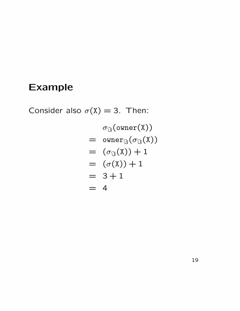
Example

Consider also σ(X) = 3. Then:

σ�(owner(X))= owner�(σ�(X))= (σ�(X)) + 1

= (σ(X)) + 1

= 3 + 1

= 4

19

Example

Consider � as before.

Then:

� |= owns(volvo, volvo) ⊃ happy(volvo)

iff

� |= owns(volvo, volvo)

or

� |= happy(volvo)

iff

〈σ�(volvo), σ�(volvo)〉 ∈ owns�or

σ�(volvo) ∈ happy�iff

〈0,0〉 ∈ owns� or 0 ∈ happy�iff

0 > 0 or 0 = 0

iff

true

22

Models

Let F be a closed formula.

Let P be a set of closed formulas.

An interpretation � is a model of F iff � |= F .

An interpretation � is a model of P iff � is a

model of every formula in P .

Satisfiability

F (resp. P) is satisfiable iff F (resp. P) have

at least one model. (Otherwise F/P is

unsatisfiable.)

23

Example

� (defined as before) is a model of:

owns(owner(volvo), volvo)

and:

∀X(owns(X, volvo) ⊃ happy(X))

24

Logical consequence

F is a logical consequence of P (P |= F) iff F

is true in all of P ’s models

(Mod(P) ⊆Mod(F)).

Theorem

P |= F iff P ∪ {¬F} is unsatisfiable.

25

Logical equivalence

Let F, G,∀XH(X) be formulas.

F and G are logically equivalent (F ≡ G) iff

� |=σ F exactly when � |=σ G.

F ⊃ G ≡ ¬F ∨G

F ⊃ G ≡ ¬G ⊃ ¬F

F ↔ G ≡ (F ⊃ G) ∧ (G ⊃ F)

¬(F ∧G) ≡ ¬F ∨ ¬G

¬(F ∨G) ≡ ¬F ∧ ¬G

¬∀XH(X) ≡ ∃X¬H(X)

¬∃XH(X) ≡ ∀X¬H(X)

In addition, if X does not occur free in F .

∀X(F ∨H(X)) ≡ F ∨ ∀XH(X)

26

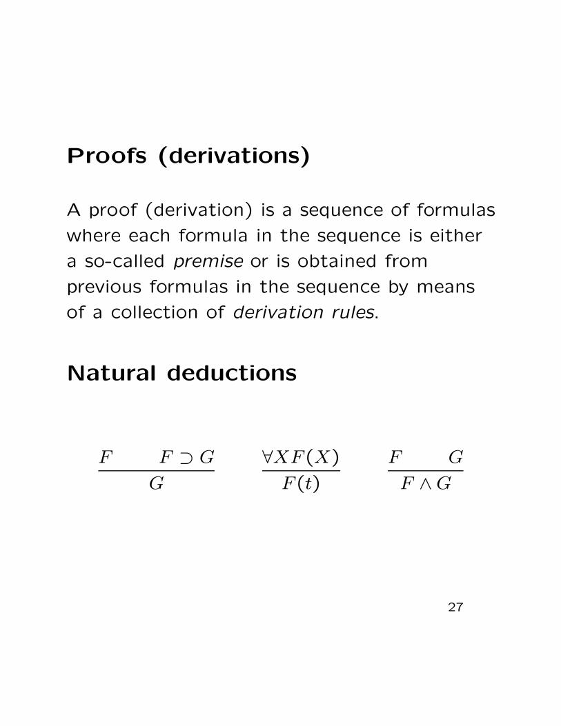
Proofs (derivations)

A proof (derivation) is a sequence of formulas

where each formula in the sequence is either

a so-called premise or is obtained from

previous formulas in the sequence by means

of a collection of derivation rules.

Natural deductions

F F ⊃ G

G

∀XF(X)

F(t)

F G

F ∧G

27

Example

1. owns(owner(volvo), volvo) P2. ∀X(owns(X, volvo) ⊃ happy(X)) P3. owns(owner(volvo), volvo) ⊃ happy(owner(volvo)))4. happy(owner(volvo))

28

Proofs

Let P be a set of closed formulas (premises)

Let F be a closed formula.

We write P � F when there is a derivation of

F from the premises P .

Soundness and completeness

If P � F then P |= F . (soundness)

If P |= F then P � F . (completeness)

29

Definite Programs: Overview

• Definite programs:

– Rules;

– Facts;

– Goals.

• Herbrand-interpretations;

• Herbrand-models;

• Fixpoint-semantics.

30

Clauses

A clause is a formula:

∀(A1 ∨ . . . ∨Am ∨ ¬Am+1 ∨ . . . ∨ ¬Am+n)

where A1, . . . , Am, Am+1, . . . , Am+n are atoms

and m, n ≥ 0.

∀(A1 ∨ . . . ∨Am ∨ ¬Am+1 ∨ . . . ∨ ¬Am+n)

≡∀((A1 ∨ . . . ∨Am) ∨ ¬(Am+1 ∧ . . . ∧Am+n))

≡∀((A1 ∨ . . . ∨Am)← (Am+1 ∧ . . . ∧Am+n))

31

Definite clauses

A definite clause is a clause where m ≤ 1:

Rules

A rule is a clause where m = 1 and n > 0:

∀(A1 ← A2 ∧ . . . ∧Am+n)

Facts

A fact is a clause where m = 1 and n = 0:

∀(A1)

32

(Definite) goals

A goal is a clause where m = 0 and n ≥ 0:

∀(¬(A1 ∧ . . . ∧Am+n))

A goal where m = n = 0 is called the empty

goal.

Notation

Rules: A1 ← A2, . . . , An+1. n > 0Facts: A1.Goals: ← A1, . . . , An. n > 0

� n = 0

33

Logic Programming Anatomy

head neck bodyA0 ← A1, . . . , An

34

Logic programs

A definite program is a finite set of rules and

facts.

A definite program P is used to answer

“existential questions” (queries) such as:

“are there any odd integers?”

The query can be answered “yes” if e.g:

P |= ∃X odd(X)

This is equivalent to proving that:

P ∪ {¬∃X odd(X)}is unsatisfiable (has no models).

35

Resolution

Note that ¬∃(A1 ∧ . . . ∧An) is equivalent to

∀¬(A1 ∧ . . . ∧An). That is, a goal.

Resolution is used to prove that a set of

clauses is unsatisfiable. As a side-effect

resolution produces “witnesses” (variable

bindings). See chapter 3.

36

Herbrand interpretations

Let P be a logic program based on the

vocabulary A

Herbrand universe

The Herbrand universe of P (A really) is the

set of all ground terms that can be built

using constants and functors in P (A).

Denoted UP (UA).

Herbrand base

The Herbrand base of P (A) is the set of all

ground atoms that can be built using UP and

the predicate symbols of P (A). Denoted BP

(BA).

37

Example

Vocabulary:


Herbrand universe:

UA = {volvo, owner(volvo), owner(owner(volvo)), . . .}

Herbrand base:

BA = {happy(s) | s ∈ UA}∪{owns(s, t) | s, t ∈ UA}

38

Herbrand interpretations

A Herbrand interpretation of P is an

interpretation � where |�| = UP and where:

• c� = c for every constant c;

• f�(t1, . . . , tn) = f(t1, . . . , tn) for every

functor f/n;

• p� is a subset of UP × · · · × UP︸︷︷︸n

for every

predicate symbol p/n.

That is, the interpretation of a ground term

is the term itself!

39

Observation I

Since all ground terms are interpreted as

themselves, it is sufficient to specify the

interpretation of the predicate symbols when

describing a Herbrand interpretation; in other

words, to specify a Herbrand interpretation �it is sufficient to specify, for each predicate

symbol, the set:

{〈t1, . . . , tn〉 ∈ UnP | p(t1, . . . , tn) is true in �}

Observation II

Instead of describing a Herbrand

interpretation � as a family of sets we usually

describe � as a single set of all ground atoms

that are true in �.� = {p(t1, . . . , tn) | p(t1, . . . , tn) is true in �}

40

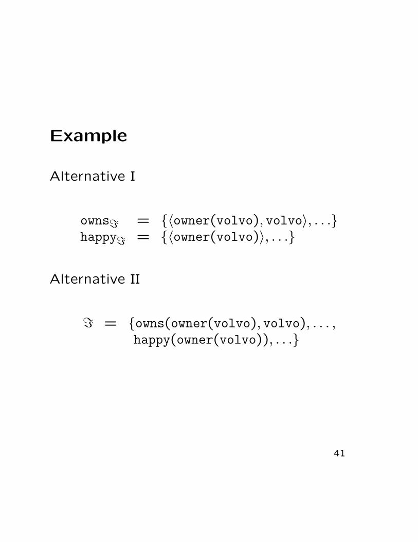
Example

Alternative I

owns� = {〈owner(volvo), volvo〉, . . .}happy� = {〈owner(volvo)〉, . . .}

Alternative II

� = {owns(owner(volvo), volvo), . . . ,happy(owner(volvo)), . . .}

41

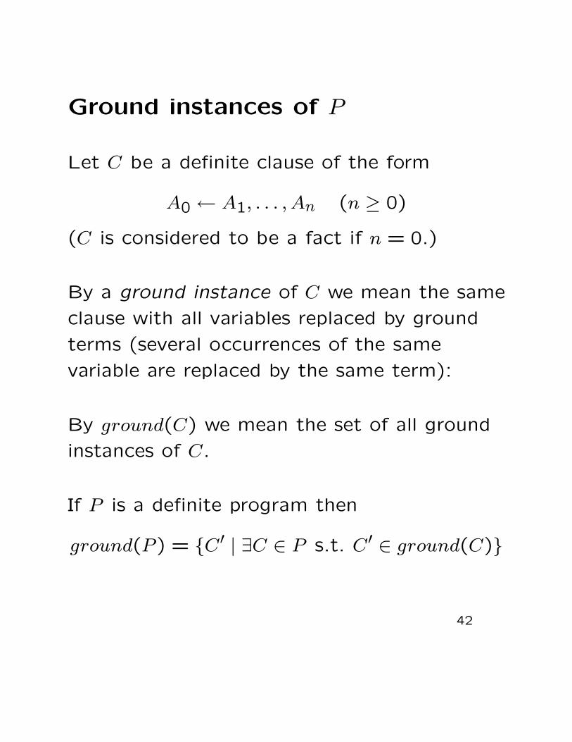
Ground instances of P

Let C be a definite clause of the form

A0← A1, . . . , An (n ≥ 0)

(C is considered to be a fact if n = 0.)

By a ground instance of C we mean the same

clause with all variables replaced by ground

terms (several occurrences of the same

variable are replaced by the same term):

By ground(C) we mean the set of all ground

instances of C.

If P is a definite program then

ground(P) = {C ′ | ∃C ∈ P s.t. C ′ ∈ ground(C)}

42

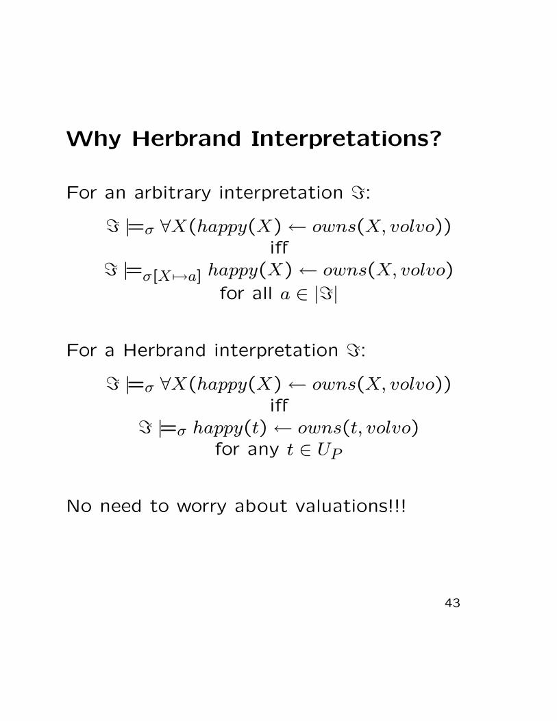
Why Herbrand Interpretations?

For an arbitrary interpretation �:� |=σ ∀X(happy(X)← owns(X, volvo))

iff� |=σ[X �→a] happy(X)← owns(X, volvo)

for all a ∈ |�|

For a Herbrand interpretation �:� |=σ ∀X(happy(X)← owns(X, volvo))

iff� |=σ happy(t)← owns(t, volvo)

for any t ∈ UP

No need to worry about valuations!!!

43

Herbrand models

A Herbrand model of F (resp. P) is a

Herbrand interpretation which is a model of F

(resp. all formulas in P).

Observation

A ground atom A is true in a Herbrand

interpretation � iff A ∈ �.

Theorem

Let P be a set of definite clauses

(facts/rules/goals) and M be an arbitrary

model of P . Then:

� := {A ∈ BP |M |= A}is a Herbrand model of P .

44

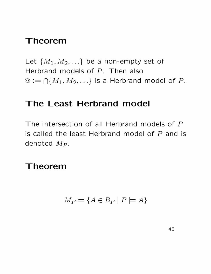
Theorem

Let {M1, M2, . . .} be a non-empty set of

Herbrand models of P . Then also

� :=⋂{M1, M2, . . .} is a Herbrand model of P .

The Least Herbrand model

The intersection of all Herbrand models of P

is called the least Herbrand model of P and is

denoted MP .

Theorem

MP = {A ∈ BP | P |= A}

45

“Construction” of MP

Observation

In order for � to be a model of P it isrequired that:

• If A is a ground instance of a fact thenA ∈ �, and

• If A← A1, . . . , An is a ground instance of aclause in P and {A1, . . . , An} ⊆ � thenA ∈ �.

Immediate consequence operator

TP (x) :=

{A ∈ BP | A← A1, . . . , An ∈ ground(P)

and {A1, . . . , An} ⊆ x}46

Theorem

MP = TnP (∅) when n→∞

47

Example

gp(X,Y) :- p(X,Z), p(Z,Y).

p(X,Y) :- f(X,Y).

p(X,Y) :- m(X,Y).

f(adam,bill).

f(adam,carol).

f(bill,eve).

m(carol,david).

48

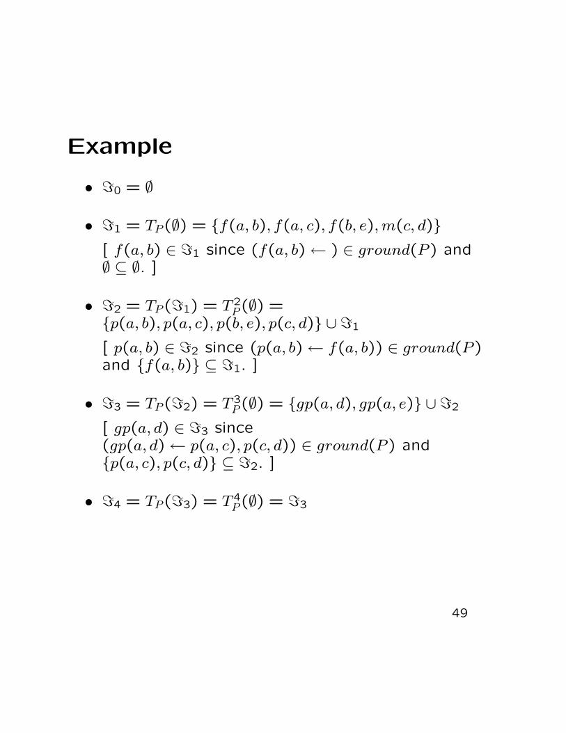
Example

• �0 = ∅

• �1 = TP(∅) = {f(a, b), f(a, c), f(b, e), m(c, d)}[ f(a, b) ∈ �1 since (f(a, b)← ) ∈ ground(P ) and∅ ⊆ ∅. ]

• �2 = TP(�1) = T 2P(∅) =

{p(a, b), p(a, c), p(b, e), p(c, d)} ∪ �1

[ p(a, b) ∈ �2 since (p(a, b)← f(a, b)) ∈ ground(P )and {f(a, b)} ⊆ �1. ]

• �3 = TP(�2) = T 3P(∅) = {gp(a, d), gp(a, e)} ∪ �2

[ gp(a, d) ∈ �3 since(gp(a, d)← p(a, c), p(c, d)) ∈ ground(P ) and{p(a, c), p(c, d)} ⊆ �2. ]

• �4 = TP(�3) = T 4P(∅) = �3

49

SLD-Resolution: Overview

• Substitutions;

• Unification;

• SLD-derivations;

• Soundness and completeness.

50

Substitutions

A substitution is a finite set

{X1/t1, . . . , Xn/tn} where:

• every ti is a term;

• every Xi is a variable distinct from ti;

• if i = j then Xi = Xj.

The empty substitution {} is denoted ε.

51

Let θ be a substitution {X1/t1, . . . , Xn/tn}.

Domain and Range

The domain Dom(θ) of θ is {X1, . . . , Xn} and

the range Range(θ) is the set of all variables

occurring in t1, . . . , tn.

Application

Let E be a term or formula. The application

Eθ of θ to E is the term/formula obtained

from E by simultaneously replacing all

occurrences of Xi by ti.

Eθ is called an instance of E.

52

Composition

Let θ := {X1/s1, . . . , Xm/sm} and

σ := {Y1/t1, . . . , Yn/tn} be substitutions. The

composition θσ of θ and σ is the substitution

obtained from

{X1/s1σ, . . . , Xm/smσ, Y1/t1, . . . , Yn/tn}by removing all Xi/siσ where Xi = siσ and all

Yi/ti where Yi ∈ Dom(θ).

More general substitution

A substitution θ is more general than σ

(σ � θ) iff there exists a substitution ω such

that θω = σ.

53

Theorem

Let θ, σ and γ be substitutions and E a

term/formula. Then

• (θσ)γ = θ(σγ);

• E(θσ) = (Eθ)σ;

• εθ = θε = θ.

54

Unification

A structure is a term or an atomic formula.

Unifier

A unifier of two structures s and t is a

substitution θ such that sθ = tθ.

Most general unifier (mgu)

A unifier θ of s and t is called a most general

unifier of s and t iff σ � θ for every unifier σ

of s and t. NB: Two unifiable structures have

at least one mgu (usually infinitely many).

55

Solved form

A set of equation {s1 .= t1, . . . , sn

.= tn} is in

solved form iff s1, . . . , sn are distinct variables

none of which occur in t1, . . . , tn.

Solution

A substitution θ is a solution to a set of

equations {s1 .= t1, . . . , sn

.= tn} iff θ is a

unifier of si and ti (1 ≤ i ≤ n).

Theorem

If {X1.= t1, . . . , Xn

.= tn} is in solved form

then {X1/t1, . . . , Xn/tn} is an mgu of Xi and

ti (1 ≤ i ≤ n).

56

select an arbitrary s.= t ∈ E ;

case s.= t of

f(s1, . . . , sn).= f(t1, . . . , tn)

where n ≥ 0 ⇒replace equation by s1

.= t1, . . . , sn

.= tn;

f(s1, . . . , sm).= g(t1, . . . , tn)

where f/m = g/n ⇒halt with ⊥;

X.= X ⇒remove the equation;

t.= X where t is not a variable ⇒

replace equation by X.= t;

X.= t where X = t and X has more than

one occurrence in E ⇒if X is a proper subterm of t then

halt with ⊥else

replace all other occurrences

of X by t;

esac

57

Theorem

The algorithm always terminates. If s and t

are unifiable then the algorithm returns a

solved form whose mgu is an mgu of s and t.

Otherwise the algorithm returns ⊥.

Renaming

A substitution θ := {X1/Y1, . . . , Xn/Yn} where

Y1, . . . , Yn is a permutation of X1, . . . , Xn is

called a renaming. The substitution

{Y1/X1, . . . , Yn/Xn} is called the inverse of θ

(denoted θ−1).

58

Theorem

Let θ and σ be mgu’s of s and t. Then there

exists a renaming γ such that θγ = σ (and

σγ−1 = θ).

Theorem

If θ is an mgu of s and t and σ a renaming,

then θσ is also an mgu of s and t.

59

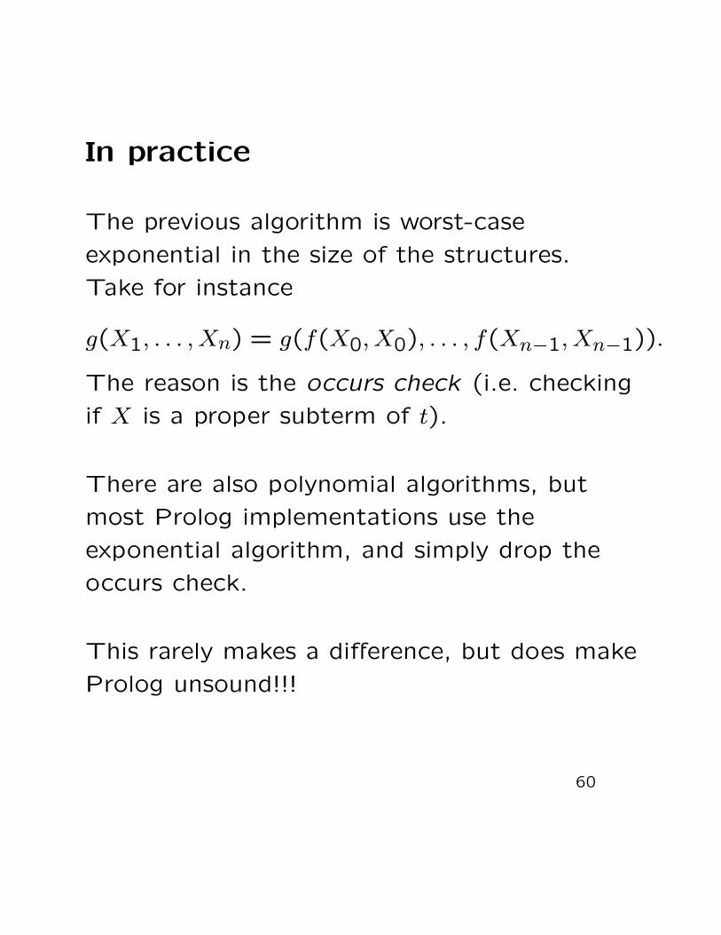
In practice

The previous algorithm is worst-case

exponential in the size of the structures.

Take for instance

g(X1, . . . , Xn) = g(f(X0, X0), . . . , f(Xn−1, Xn−1)).

The reason is the occurs check (i.e. checking

if X is a proper subterm of t).

There are also polynomial algorithms, but

most Prolog implementations use the

exponential algorithm, and simply drop the

occurs check.

This rarely makes a difference, but does make

Prolog unsound!!!

60

SLD-resolution rule

Let H ← B1, . . . , Bn be a program clause

renamed apart from ← A1, . . . , Ai, . . . , Am, and

let θ be an mgu of Ai and H. Then:

← A1, . . . , Ai, . . . , Am H ← B1, . . . , Bn

← (A1, . . . , Ai−1, B1, . . . , Bn, Ai+1, . . . , Am)θ

61

SLD-derivation

Let G0 be a goal. An SLD-derivation of G0 is

a finite/infinite sequence:

G0C0� G1 · · ·Gn−1

Cn−1� Gn · · ·

of goals and (renamed) program clauses such

that:Gi Ci

Gi+1

62

gp(X,Y) :- p(X,Z), p(Z,Y).

p(X,Y) :- f(X,Y).

p(X,Y) :- m(X,Y).

f(adam,tom).

f(adam,mary).

f(tom,david).

m(mary,anne).

63

inv(0,1).

inv(1,0).

and(0,0,0).

and(0,1,0).

and(1,0,0).

and(1,1,1).

nand(X,Y,Z) :- and(X,Y,W), inv(W,Z).

64

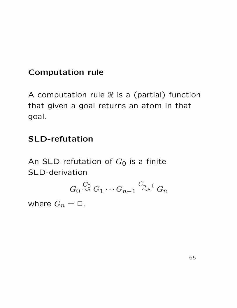
Computation rule

A computation rule � is a (partial) function

that given a goal returns an atom in that

goal.

SLD-refutation

An SLD-refutation of G0 is a finite

SLD-derivation

G0C0� G1 · · ·Gn−1

Cn−1� Gn

where Gn = �.

65

Failed derivation

A finite SLD-derivation

G0C0� G1 · · ·Gn−1

Cn−1� Gn

is said to be failed if the selected atom in Gn

does not unify with any program clause head.

Complete SLD-derivation

An SLD-derivation is complete if it is a

refutation, a failed or infinite derivation.

66

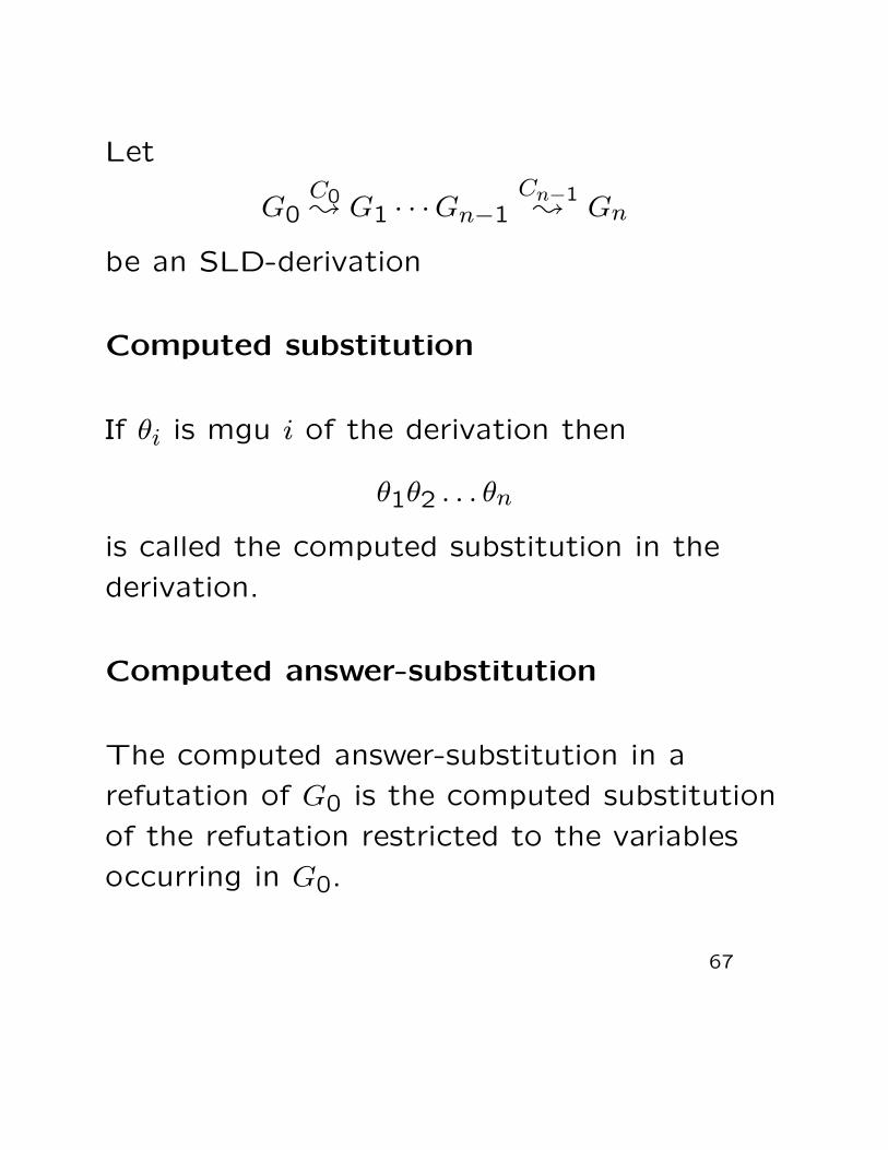
Let

G0C0� G1 · · ·Gn−1

Cn−1� Gn

be an SLD-derivation

Computed substitution

If θi is mgu i of the derivation then

θ1θ2 . . . θn

is called the computed substitution in the

derivation.

Computed answer-substitution

The computed answer-substitution in a

refutation of G0 is the computed substitution

of the refutation restricted to the variables

occurring in G0.

67

Let P be a logic program;

Let � be a computation rule

SLD-tree

The SLD-tree of a goal G0 is a tree where

• the root of the tree is G0;

• if Gi is a node in the tree then Gi has a

child Gi+1 (connected via a branch

labelled “Ci”) iff there exists an

SLD-derivation

G0C0� G1 · · ·Gi

Ci� Gi+1

with the computation rule �.

68

Soundness and completeness

Theorem (soundness)

Let P be a logic program, � a computation

rule and θ an �-computed answer-substitution

of the goal ← A1, . . . , An. Then

∀((A1 ∧ . . . ∧An)θ) is a logical consequence of

P .

Theorem (completeness)

Let P be a logic program and � a

computation rule. If ∀(A1 ∧ . . . ∧An)σ is a

logical consequence of P then there is a

refutation of ← A1, . . . , An with �-computed

answer-substitution θ such that

(A1 ∧ . . . ∧An)σ is an instance of

(A1 ∧ . . . ∧An)θ.

69

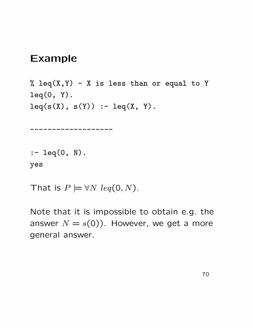
Example

% leq(X,Y) - X is less than or equal to Y

leq(0, Y).

leq(s(X), s(Y)) :- leq(X, Y).

-------------------

:- leq(0, N).

yes

That is P |= ∀N leq(0, N).

Note that it is impossible to obtain e.g. the

answer N = s(0)). However, we get a more

general answer.

70

Negation: Overview

• Closed World Assumption;

• Negation as Failure;

• Completion;

• SLDNF-resolution (part I);

• General (alt. normal) logic programs;

• Stratified logic programs;

• SLDNF-resolution (part II).

71

Program:

parent(a,b).

parent(a,c).

parent(c,d).

female(a).

female(d).

mother(X) :- parent(X,Y), female(X).

Least Herbrand model:

parent(a,b).

parent(a,c).

parent(c,d).

female(a).

female(d).

mother(a).

72

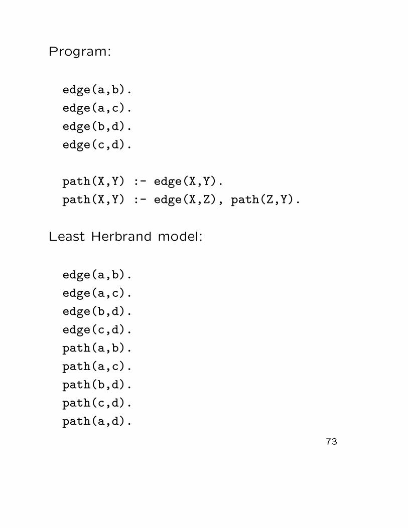
Program:

edge(a,b).

edge(a,c).

edge(b,d).

edge(c,d).

path(X,Y) :- edge(X,Y).

path(X,Y) :- edge(X,Z), path(Z,Y).

Least Herbrand model:

edge(a,b).

edge(a,c).

edge(b,d).

edge(c,d).

path(a,b).

path(a,c).

path(b,d).

path(c,d).

path(a,d).

73

Closed World Assumption

Background Definite programs can only be

used to describe positive knowledge; it is not

possible to describe objects that are not

related.

Solution I Closed world assumption:

P |= A

¬A

Problem P |= A is undecidable.

74

Negation as (finite) Failure

Solution II An SLD-tree is finitely failed iff it

is finite and does not contain any refutations.

Observation If ← A has a finitely failed

SLD-tree then P |= A. (Follows from the

soundness and completeness of

SLD-resolution.)

The NAF rule

← A has a finitely failed SLD-tree

¬A

Problem The NAF rule is not sound.

75

Completion

Thesis The program contains information

that is not written out explicitly. The

completed program is the program obtained

after addition of the missing information.

Observation {a← b, a← c} ≡ {a← b ∨ c}.

Principle An implication a← b is replaced by

an equivalence a↔ b.

76

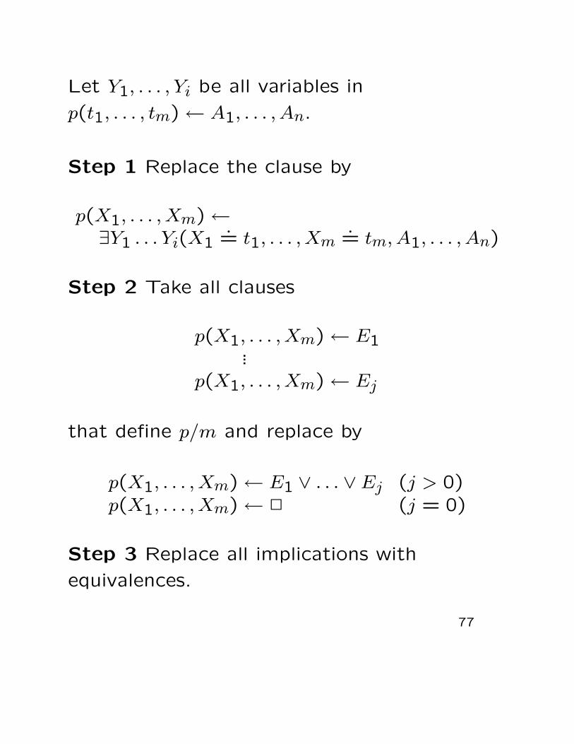
Let Y1, . . . , Yi be all variables in

p(t1, . . . , tm)← A1, . . . , An.

Step 1 Replace the clause by

p(X1, . . . , Xm)←∃Y1 . . . Yi(X1

.= t1, . . . , Xm

.= tm, A1, . . . , An)

Step 2 Take all clauses

p(X1, . . . , Xm)← E1...

p(X1, . . . , Xm)← Ej

that define p/m and replace by

p(X1, . . . , Xm)← E1 ∨ . . . ∨ Ej (j > 0)p(X1, . . . , Xm)← � (j = 0)

Step 3 Replace all implications with

equivalences.

77

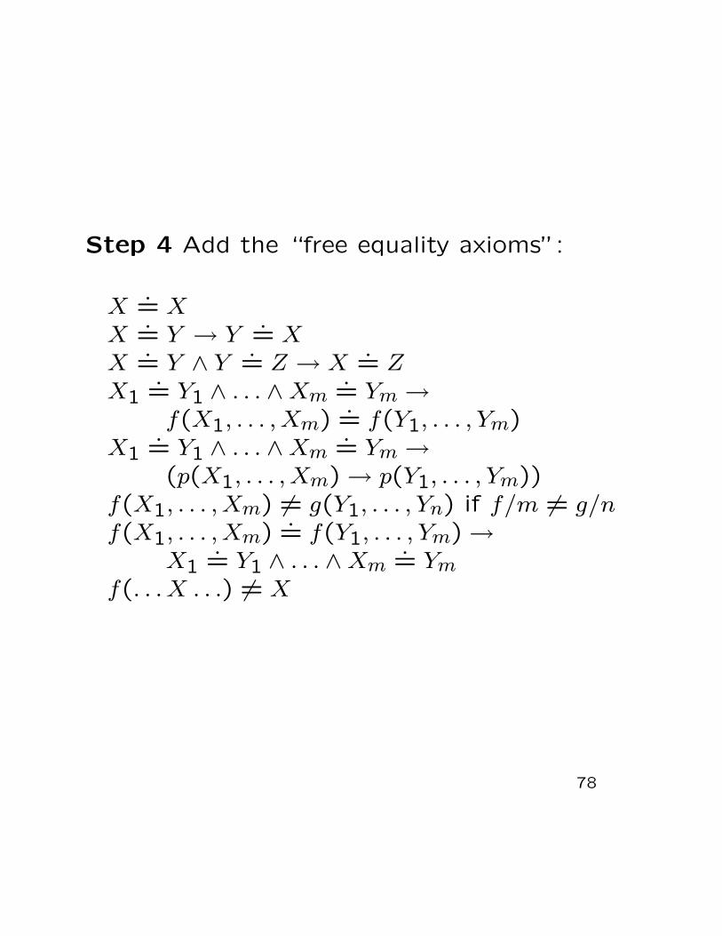
Step 4 Add the “free equality axioms”:

X.= X

X.= Y → Y

.= X

X.= Y ∧ Y

.= Z → X

.= Z

X1.= Y1 ∧ . . . ∧Xm

.= Ym→

f(X1, . . . , Xm).= f(Y1, . . . , Ym)

X1.= Y1 ∧ . . . ∧Xm

.= Ym→

(p(X1, . . . , Xm)→ p(Y1, . . . , Ym))f(X1, . . . , Xm) = g(Y1, . . . , Yn) if f/m = g/nf(X1, . . . , Xm)

.= f(Y1, . . . , Ym)→

X1.= Y1 ∧ . . . ∧Xm

.= Ym

f(. . . X . . .) = X

78

Soundness of “Negation as Failure”

Theorem Let P be a definite program. If

← A has a finitely failed SLD-tree then

comp(P) |= ∀¬A.

Completeness of “Negation as Failure”

Theorem Let P be a definite program. If

comp(P) |= ∀¬A then there exists a finitely

failed SLD-tree of ← A.

79

SLDNF-resolution for definite programs

A general goal is an expression

← L1, . . . , Ln.

where each Li is an atom (positive literal) or

a negated atom (negative literal).

Combine SLD-resolution and “Negation

as Failure”

Given a general goal — if the selected literal

is positive then the next goal is obtained in

the usual way. If the selected literal is

negative (¬A) and ← A has a finitely failed

SLD-tree then the next goal is obtained by

removing ¬A from the goal.

80

Soundness of SLDNF

Theorem Let P be a definite program and

← L1, . . . , Ln a general goal. If ← L1, . . . , Ln

has an SLDNF-refutation with computed

answer-substitution θ then ∀(L1 ∧ · · · ∧ Ln)θ is

a logical consequence of comp(P).

No completeness!!!

81

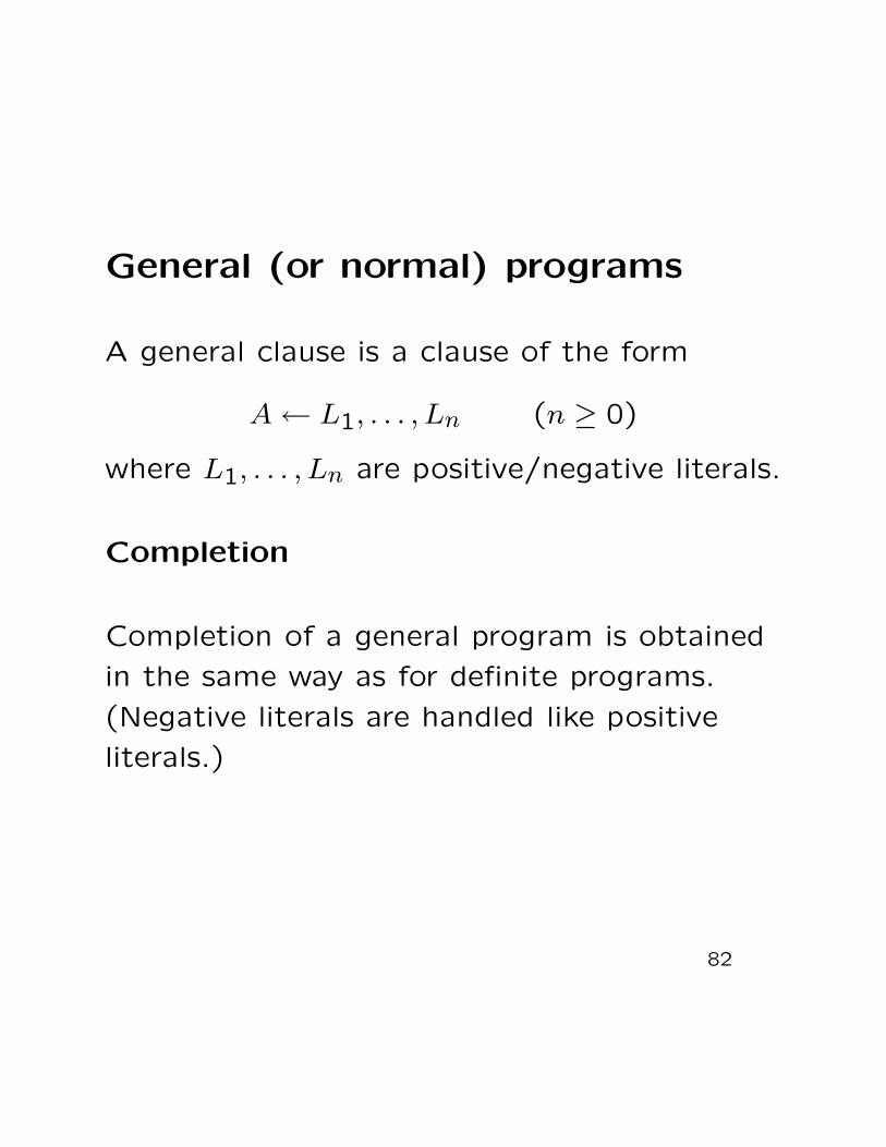
General (or normal) programs

A general clause is a clause of the form

A← L1, . . . , Ln (n ≥ 0)

where L1, . . . , Ln are positive/negative literals.

Completion

Completion of a general program is obtained

in the same way as for definite programs.

(Negative literals are handled like positive

literals.)

82

Stratified programs

Problem Completion of a general program

can be inconsistent (unsatisfiable).

Limitation A stratified program is a general

program where “no relation is defined in

terms of its own complement”. That is, no

predicate symbol depends on its own

negation.

83

Stratified programs

A general program P is stratified iff there

exists a partitioning P1, . . . , Pn of P such that

• if p(. . .)← . . . , q(. . .), . . . ∈ Pi then

DEF(q) ⊆ P1 ∪ . . . ∪ Pi.

• if p(. . .)← . . . ,¬q(. . .), . . . ∈ Pi then

DEF(q) ⊆ P1 ∪ . . . ∪ Pi−1.

Theorem Completion of a stratified program

is always consistent.

84

SLDNF-resolution for generalprograms

Let P be a general program, G0 a general

goal and � a computation rule. The

SLDNF-forest of G0 is the least forest

(modulo renaming) such that

1. G0 is a root of one tree.

2. if G is a node and �(G) = A then G has a

child G′ for each clause C such that G′ isobtained from G and C. If there is no

such clause, G has a single child FF;

3. if G is a node of the form

← L1, . . . , Li−1,¬A, Li+1, . . . , Li+j and

�(G) = ¬A, then

85

Cont’d

• the forest contains a tree with the root

← A;

• if the tree with the root ← A has a leaf �

with the empty computed

answer-substitution, then G has a child

FF.

• if the tree with root ← A is finite and all

leaves are FF, then G has a single child

← L1, . . . , Li−1, Li+1, . . . , Li+j.

86

Soundness of SLDNF-resolution

Let P be a general program, ← L1, . . . , Ln a

general goal and � a computation rule. If θ is

a computed answer-substitution in an

SLDNF-refutation of ← L1, . . . , Ln then

∀((L1 ∧ . . . ∧ Ln)θ) is a logical consequence of

comp(P).

87

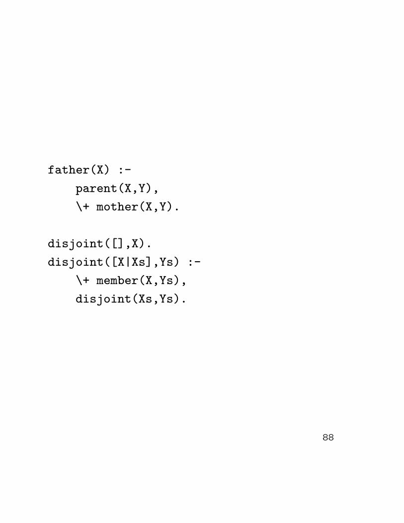
father(X) :-

parent(X,Y),

\+ mother(X,Y).

disjoint([],X).

disjoint([X|Xs],Ys) :-

\+ member(X,Ys),

disjoint(Xs,Ys).

88

founding(X) :-

on(Y,X),

on_ground(X).

on_ground(X) :-

\+ off_ground(X).

off_ground(X) :-

on(X,Y).

on(c,b).

on(b,a).

89

go_well_together(X,Y) :-

\+ incompatible(X,Y).

incompatible(X,Y) :-

\+ likes(X,Y).

incompatible(X,Y) :-

\+ likes(Y,X).

likes(X,Y) :-

harmless(Y).

likes(X,Y) :-

eats(X,Y).

harmless(rabbit).

eats(python,rabbit).

90

father(X,Y) :-

parent(X,Y),

\+ mother(X,Y).

parent(a,b).

parent(c,b).

mother(a,b).

91

father(X,Y) :-

parent(X,Y),

\+ mother(X,Y).

mother(X,Y) :-

parent(X,Y),

\+ father(X,Y).

parent(a,b).

parent(c,b).

92

on_top(X) :-

\+ blocked(X).

blocked(X) :-

on(Y,X).

on(a,b).

%---------------------

| ?- \+ on_top(b).

| ?- \+ on_top(X).

93

Logic and Grammars: Overview

• Context free languages;

• Context sensitive languages;

• Definite Clause Grammars (DCGs);

• DCGs and Prolog.

94

Context free languages

• A context free grammar is a triple

〈N, T, P 〉 where:

– N is a finite set of non-terminals;

– T is a finite set of terminals (and

N ∩ T = ∅);

– P ⊆ N × (N ∪ T)∗ is a finite set of

production rules.

• Examples of production rules:

〈expr〉 → 〈expr〉+ 〈expr〉〈sent〉 → 〈np〉〈vp〉

95

Derivations

• Let α, β, γ ∈ (N ∪ T)∗. We say that αAγ

directly derives αβγ iff A→ β ∈ P .

Denoted

αAγ ⇒ αβγ

• We say that α1 derives αn iff there exists

a sequence

α1⇒ α2, α2 ⇒ α3, . . . , αn−1 ⇒ αn. Denoted

α1∗⇒ αn

• A terminal string α ∈ T ∗ is in the language

of A iff A∗⇒ α.

96

Example: Context free grammar

〈sent〉 → 〈np〉〈vp〉〈np〉 → the 〈n〉〈vp〉 → runs

〈n〉 → engine

〈n〉 → rabbit

97

Naive implementation

sent(Z)← append(X, Y, Z), np(X), vp(Y ).np([the|X])← n(X).vp([runs]).n([engine]).n([rabbit]).

append([ ], Xs, Xs).append([X|Xs], Y s, [X|Zs])←

append(Xs, Y s, Zs).

98

Usage of “Difference Lists”

• Assume that “−/2” denotes a partial

function which given two strings

x1 . . . xm−1xm . . . xn and xm . . . xn returns

the string x1 . . . xm−1.

• Example

sent(X0–X2)← np(X0–X1), vp(X1–X2).

x1 . . . xi−1 xi . . . xj−1 xj . . . xk︸︷︷︸X2︸︷︷︸

X1︸︷︷︸X0

99

Two Alternatives

sent(X0–X2)← np(X0–X1), vp(X1–X2).np(X0–X2)← ’C’(X0, the, X1), n(X1–X2).vp(X0–X1)← ’C’(X0, runs, X1).n(X0–X1)← ’C’(X0, engine, X1).n(X0–X1)← ’C’(X0, rabbits, X1).’C’([X|Y ], X, Y ).

sent(X0–X2)← np(X0–X1), vp(X1–X2).np([the|X1]–X2)← n(X1–X2).vp([runs|X1]–X1).n([engine|X1]–X1).n([rabbit|X1]–X1).

100

Partial deduction

grandparent(X,Y) :-

parent(X,Z), parent(Z,Y).

-----------

parent(X,Y) :-

father(X,Y).

parent(X,Y) :-

mother(X,Y).

%-------------------------------------

grandparent(X,Y) :-

father(X,Z), parent(Z,Y).

grandparent(X,Y) :-

mother(X,Z), parent(Z,Y).

parent(X,Y) :-

father(X,Y).

parent(X,Y) :-

mother(X,Y).

101

Context sensitive languages

• Some languages cannot be described by

context free grammars. For instance

ABC = {anbncn | n ≥ 0}= {ε, abc, aabbcc, aaabbbccc, . . .}

• The language ABC can be expressed in

Prolog

abc(X0–X3)←a(N, X0–X1),b(N, X1–X2),c(N, X2–X3).

a(0, X0–X0).a(s(N), [a|X1]–X2)← a(N, X1–X2).b(0, X0–X0).b(s(N), [b|X1]–X2)← b(N, X1–X2).c(0, X0–X0).c(s(N), [c|X1]–X2)← c(N, X1–X2).

102

Definite Clause Grammars (DCGs)

• A Definite Clause Grammar is a triple

〈N, T, P 〉 where

– N is a finite/infinite set of atoms;

– T is a finite/infinite set of terms (and

N ∩ T = ∅);

– P ⊆ N × (N ∪ T)∗ is a finite set of

production rules.

103

Derivations

• Let α, β, γ ∈ (N ∪ T)∗. We say that αAγ

directly derives (αβγ)θ iff A′ → β ∈ P and

mgu(A, A′) = θ. Denoted

αAγ ⇒ (αβγ)θ

• We say that α1 derives αn (denoted

α1∗⇒ αn) iff there exists a sequence

α1 ⇒ α2, α2 ⇒ α3, . . . , αn−1⇒ αn

• A terminal string α ∈ T ∗ is in the language

of A iff A∗⇒ α.

104

Example of DCG

sent(s(X,Y)) --> np(X, N)\ vp(Y, N).

np(john, singular(3)) --> [john].

np(they,plural(3)) --> [they].

vp(run,plural(X)) --> [run].

vp(runs,singular(3)) --> [runs].

105

Semantical (context sensitive)constraints

The following DCG describes the language

{a2nb2nc2n | n ≥ 0}

abc --> a(N), b(N), c(N), even(N).

a(0) --> [].

a(s(N)) --> [a], a(N).

...

even(0) --> [].

even(s(s(N))) --> even(N).

106

Note

• The language of even(X) contains only

the string ε!!!

• This may be emphasized by writing

abc --> a(N), b(N), c(N), {even(N)}.

• and by defining even/1 as a logic program

even(0).even(s(s(X)))← even(X).

107

DCGs and Prolog

• Every production rule in a DCG can be

compiled into a Prolog clause;

• The resulting Prolog program can be used

as a (top-down) parser for the language

(cf. “recursive descent”);

108

Compilation

• Assume that X0, . . . , Xm are distinct

variables that do not occur in

p(t1, . . . , tn) → T1, . . . , Tm

• The Prolog program will then contain a

clause

p(t1, . . . , tn, X0, Xm)← T ′1, . . . , T ′m.

where each T ′i , (1 ≤ i ≤ m), is of the form

q(t1, . . . , tn, Xi−1, Xi) if Ti = q(t1, . . . , tn)’C’(Xi−1, t, Xi) if Ti = [t]

T, Xi−1 = Xi if Ti = {T}Xi−1 = Xi if Ti = [ ]

109

Example

sent --> np, vp.

np --> [the], n.

vp --> [runs].

n --> [boy].

% Translates into...

sent(S0,S2) :- np(S0,S1), vp(S1,S2).

np(S0,S2) :- ’C’(S0,the,S1), n(S1,S2).

vp(S0,S1) :- ’C’(S0,runs,S1).

n(S0,S1) :- ’C’(S0,boy,S1).

’C’([X|Xs],X,Xs).

110

Summary

• Logic programming can be used to define

– (Regular languages);

– Context free languages;

– Context sensitive languages;

– (Recursively enumerable languages).

• Definite Clause Grammars (DCGs);

• Compilation of DCGs into Prolog.

111

Examples

% Membership in a ordered binary tree

member(X, node(Left, X, Right)).

member(X, node(Left, Y, Right)) :-

X < Y,

member(X, Left).

member(X, node(Left, Y, Right)) :-

X > Y,

member(X, Right).

% Property of being a father

father(X) :-

parent(X, Y), male(X).

113

General

• Prolog constructs the SLD(NF)-tree by a

depth-first search in combination with

backtracking.

• By means of cut (!) the user can prohibit

the Prolog engine from exploring certain

branches in the tree.

• Cut (!) may only occur in the righthand

sides of clauses and can be viewed as a

regular (nullary) atom.

114

Principles

• Two principal uses

– Prune infinite and failed branches

(green cut);

– Prune refutations (red cut).

• Acceptable ”red cut”:

– Prune multiple occurrences of the

same answer.

115

The Golden Rule

First write a correct program without cuts.

Then add cuts in approprate places to

improve the efficiency.

116

Constraint logic programming

• Constraints

• Operations on constraints

• Constraint Logic Programming

– Language

– Operational semantics

– Examples

117

Constraint

Given a set of variables, a constraint is a

restriction on the possible values of the

variables.

Example

Variables: X, Y .

Constraint I: X2 + Y 2 ≤ 4

Constraint II: Y ≥ 2− 2 ·X

118

Solution

The constraint X2 + Y 2 ≤ 4 has a set of

solutions – variable assignments when the

constraint is true, e.g:

{X �→ 2, Y �→ 0}{X �→ 0, Y �→ 2}{X �→ 1, Y �→ 1}

A mapping from variables to values is called a

valuation. A valuation where the constraint is

true is called a solution.

119

Domain of a constraint

Whether a constraint has a solution or not

depends on the values that the variables can

take.

The constraint X2 = 2 has a real solution,

but not an integer or a rational solution.

The set of all possible values of the variables

is called the domain of the constraint.

120

Conjunctive constraints

The conjunction of the primitive constraints

X2 + Y 2 ≤ 4 and Y ≥ 2− 2 ·X is a new

(conjunctive) constraint:

Sets of primitive constraints represent

conjunctive constraints.

121

Properties of constraints

A constraint is said to be satisfiable iff it has

at least one solution.

A constraint C1 implies a constraint C2

(written C1 |= C2) iff every solution of C1 is

also a solution of C2.

Two constraints are equivalent if they have

the same set of solutions.

122

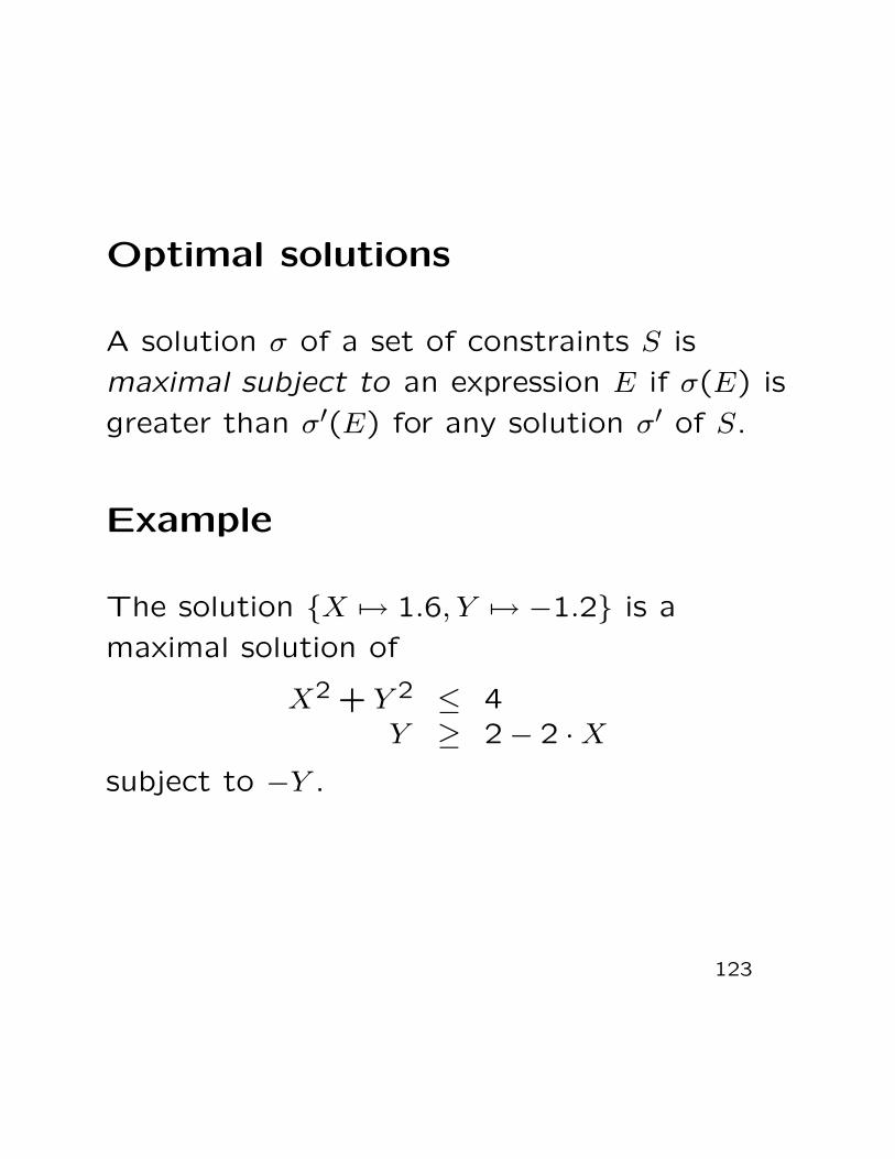
Optimal solutions

A solution σ of a set of constraints S is

maximal subject to an expression E if σ(E) is

greater than σ′(E) for any solution σ′ of S.

Example

The solution {X �→ 1.6, Y �→ −1.2} is a

maximal solution of

X2 + Y 2 ≤ 4Y ≥ 2− 2 ·X

subject to −Y .

123

Constraint Logic Programming

sorted([]).

sorted([X]).

sorted([Fst,Snd|Rst]) :-

Fst =< Snd, sorted([Snd|Rst]).

------------------------------------

:- sorted([X1,X2,X3]).

ARITHMETIC ERROR!!!

124

Language

• Functors and predicate symbols divided

into:

– Uninterpreted symbols (Herbrand

terms/atoms);

– Interpreted symbols (constraints).

• Special solvers handle constraints;

• SLD(NF)-resolution is used for Herbrand

atoms;

125

Language (cont’d.)

• A clause is an expression

A0← C1, . . . , Cm, A1, . . . , An

where

– A0, . . . , An are Herbrand atoms;

– C1, . . . , Cm are constraints.

• A goal is an expression

← C1, . . . , Cm, A1, . . . , An

126

CLP(X): A Family of Languages

CLP(R) Linear equations over reals

CLP(Q) Linear equations over rationals

CLP(B) Booleans

CLP(FD) Finite domains

127

Example CLP(R)

mortgage(Loan,Years,AInt,Bal,APay) :-

{ Years>0,

Years <= 1,

Bal=Loan*(1+Years*AInt)-APay }.

mortgage(Loan,Years,AInt,Bal,APay) :-

{ Years>1,

NewLoan = Loan*(1+AInt)-APay,

Years1 = Years-1 },

mortgage(NewLoan,Years1,AInt,Bal,APay).

-------------------------------------------

?- mortgage(120000,10,0.1,0,AnnPay).

AnnPay=19529.4

?- mortgage(Loan,10,0.1,0,19529.4).

Loan=120000

?- mortgage(Loan,10,0.1,0,AnnPay).

Loan=6.14457*AnnPay

128

Resolution with constraints

A state is a pair (G ; S) where G is a goal,

and S is a constraint store. Given a program

P a derivation is a sequence of states:

• (←A, B ; S)⇒ (←A = A′, B′, B ; S) if

A′←B′ ∈ P

• (←C, G ; S)⇒ (←G ; {C} ∪ S)

• (G ; S)⇒ fail if sat(S) = false;

• (G ; S)⇒ (G ; S′) if S and S′ areequivalent.

• (G ; {X = t} ∪ S)⇒ (G ; S){X/t}

129

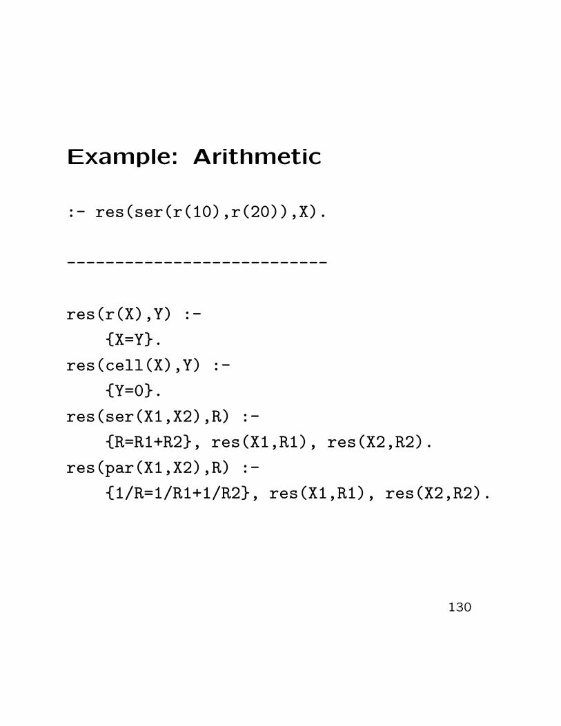
Example: Arithmetic

:- res(ser(r(10),r(20)),X).

---------------------------

res(r(X),Y) :-

{X=Y}.

res(cell(X),Y) :-

{Y=0}.

res(ser(X1,X2),R) :-

{R=R1+R2}, res(X1,R1), res(X2,R2).

res(par(X1,X2),R) :-

{1/R=1/R1+1/R2}, res(X1,R1), res(X2,R2).

130

Modeling with Boolean constraints

Boolean operations

+ Disjunktion * Conjunction=< Implikation =:= Equivalence# Exclusive or ~ Negation

MOS transistors

drain

source

gate

drain

source

gate

nmos(S,G,D) :- sat(S * G =:= D * G).

pmos(S,G,D) :- sat(S * ~G =:= D * ~G).

131

Design of XOR-gate

XY

Z

T

1

0

circuit(X,Y,Z) :-

pmos(X,Y,Z),

pmos(1,X,T),

nmos(T,X,0),

nmos(T,Y,Z),

nmos(Y,T,Z),

pmos(Y,X,Z).

132

Verification of correctness

?- circuit(X,Y,Z), taut(Z =:= X#Y, 1).

yes

133

CLP with Finite Domains

• Constraints and constraint problems

• Primitive constraints

• CLP(FD)

• Optimization

• Global constraints

134

Example

• A, B and C live in different houses

• C lives left of B

• B has two neighbors

135

Constraint problem

• A constraint problem consists of a finite

set of problem variables,

• Each variable takes its value from a given

domain

• Constraints are relations that restrict the

values that can be assigned to the

problem variables

136

Mathematical reformulation

• A, B, C ∈ {1,2,3}

• A = B, A = C and B = C

• C < B

• (A < B < C) or (C < B < A)

137

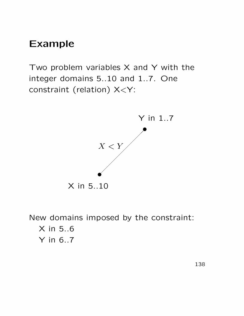
Example

Two problem variables X and Y with the

integer domains 5..10 and 1..7. One

constraint (relation) X<Y:

�

�

��

��

��

��

��

��

X < Y

X in 5..10

Y in 1..7

New domains imposed by the constraint:

X in 5..6

Y in 6..7

138

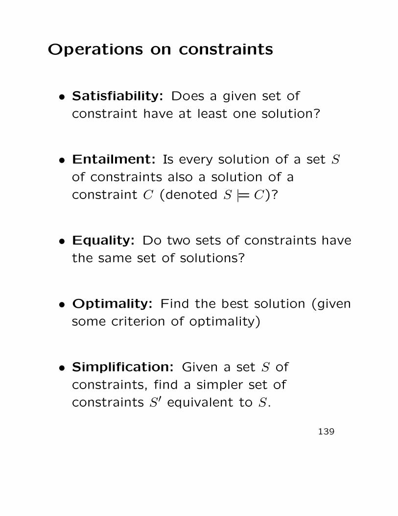
Operations on constraints

• Satisfiability: Does a given set of

constraint have at least one solution?

• Entailment: Is every solution of a set S

of constraints also a solution of a

constraint C (denoted S |= C)?

• Equality: Do two sets of constraints have

the same set of solutions?

• Optimality: Find the best solution (given

some criterion of optimality)

• Simplification: Given a set S of

constraints, find a simpler set of

constraints S′ equivalent to S.

139

Primitive Finite Domainconstraints

| ?- X in 3..8.

X in 3..8

| ?- X in 3..8, Y in 1..4, Z #= X+Y.

X in 3..8,

Y in 1..4,

Z in 4..12

| ?- X in 5..10, Y in 1..7, X #< Y.

X in 5..6,

Y in 6..7

140

Domains vs solutions

Note that domains are not identical to

solutions:

?- X in 5..10, Y in 1..7, X #< Y.

Produces the domains:

X in 5..6.

Y in 6..7.

But the domains contain all solutions:

X = 5, Y = 6

X = 5, Y = 7

X = 6, Y = 7

141

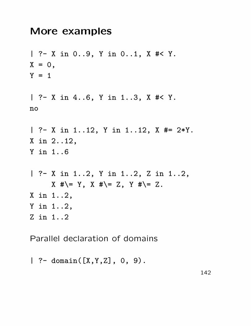
More examples

| ?- X in 0..9, Y in 0..1, X #< Y.

X = 0,

Y = 1

| ?- X in 4..6, Y in 1..3, X #< Y.

no

| ?- X in 1..12, Y in 1..12, X #= 2*Y.

X in 2..12,

Y in 1..6

| ?- X in 1..2, Y in 1..2, Z in 1..2,

X #\= Y, X #\= Z, Y #\= Z.

X in 1..2,

Y in 1..2,

Z in 1..2

Parallel declaration of domains

| ?- domain([X,Y,Z], 0, 9).

142

Labeling

Domains approximate solutions...

| ?- X in 1..2, Y in 1..3, X #< Y.

X in 1..2,

Y in 2..3

Systematically assign values to a variable

from its domain.

| ?- X in 1..2, Y in 1..3, X #< Y,

labeling([],[X,Y]).

X=1, Y=2

X=1, Y=3

X=2, Y=3

| ?- X in 1..12, Y in 1..12, X #= 2*Y,

labeling([],[X,Y]).

X=2, Y=1

X=4, Y=2

...

143

CLP(X)

A logic program is a set of rules

A0 :- A1, . . . , An

or facts

A0

where A0, A1, . . . , An are atomic formulas;

i.e. formulas of the form p(t1, . . . , tn).

Note: A constraint is an atomic formula!

A constraint logic program is a logic program

where some of A1, . . . , An may be (some

pre-defined) constraints over some algebraic

structure X.

144

CLP(X)

• CLP(R), reals

• CLP(Q), rational numbers

• CLP(B), Boolean values

• CLP(FD), finite domains

• CLP(Sets), sets

145

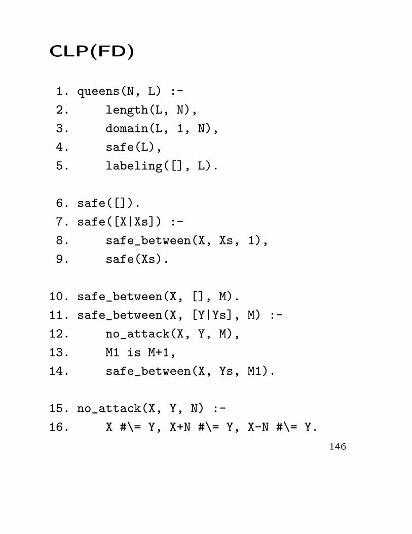
CLP(FD)

1. queens(N, L) :-

2. length(L, N),

3. domain(L, 1, N),

4. safe(L),

5. labeling([], L).

6. safe([]).

7. safe([X|Xs]) :-

8. safe_between(X, Xs, 1),

9. safe(Xs).

10. safe_between(X, [], M).

11. safe_between(X, [Y|Ys], M) :-

12. no_attack(X, Y, M),

13. M1 is M+1,

14. safe_between(X, Ys, M1).

15. no_attack(X, Y, N) :-

16. X #\= Y, X+N #\= Y, X-N #\= Y.

146

General Strategy

1. solution(L) :-

2. create_variables(L),

3. constrain_variables(L),

4. solve_constraints(L).

147

Optimization

| ?- X in 1..9, Y in 4..6, Z #= X-Y,

labeling([maximize(Z)],[X,Y]).

1. items(A,B,C,S,P) :-

2. domain([A,B,C],0,10),

3. AS #= 2*A, AP #= 3*A,

4. BS #= 3*B, BP #= 4*B,

5. CS #= 7*C, CP #= 10*C,

6. S #>= AS+BS+CS,

7. P #= AP+BP+CP,

8 . labeling([maximize(P)],[P,S,A,B,C]).

148

Global Constraints

all_different([X1, . . . , Xn])

1. smm([S,E,N,D,M,O,R,Y]) :-

2. domain([S,E,N,D,M,O,R,Y], 0, 9),

3. S #> 0, M #> 0,

4. all_different([S,E,N,D,M,O,R,Y]),

5. sum(S,E,N,D,M,O,R,Y),

6. labeling([], [S,E,N,D,M,O,R,Y]).

7. sum(S, E, N, D, M, O, R, Y) :-

8. 1000*S+100*E+10*N+D

9. +1000*M+100*O+10*R+E

10. #= 10000*M+1000*O+100*N+10*E+Y.

149

cumulative(Ss,Ds,Rs,L)

| ?- domain([S1,S2,S3],0,4),

S1 #< S3,

cumulative([S1,S2,S3],[3,4,2],[2,1,3],3),

labeling([],[S1,S2,S3]).

150

Resource allocation

1. shower(S, Done) :-

2. D = [5,3,8,2,7,3,9,3,3,5,7],

3. R = [1,1,1,1,1,1,1,1,1,1,1],

4. length(D, N),

5. length(S, N),

6. domain(S, 0, 100),

7. Done in 0..100,

8. ready(S, D, Done),

9. cumulative(S, D, R, 3),

10. labeling([minimize(Done)], [Done|S]).

11. ready([], [], _).

12. ready([S|Ss], [D|Ds], Done) :-

13. Done #>= S+D,

14. ready(Ss, Ds, Done).

151

element(X,[X1, . . . , Xn],Y )

| ?- element(X, [1,2,3,5], Y).

| ?- X in 2..3, element(X, [1, X, 4, 5], Y).

152

circuit([X1, . . . , Xn])

Traveling Salesman

X1 X2 X3 X4 X5 X6 X7X1 − 4 8 10 7 14 15X2 4 − 7 7 10 12 5X3 8 7 − 4 6 8 10X4 10 7 4 − 2 5 8X5 7 10 6 2 − 6 7X6 14 12 8 5 6 − 5X7 15 5 10 8 7 5 −

153

Traveling Salesman (cont’d)

1. tsp(Cities, Cost) :-

2. Cities = [X1,X2,X3,X4,X5,X6,X7],

3. element(X1,[ 0, 4, 8,10, 7,14,15],C1),

4. element(X2,[ 4, 0, 7, 7,10,12, 5],C2),

5. element(X3,[ 8, 7, 0, 4, 6, 8,10],C3),

6. element(X4,[10, 7, 4, 0, 2, 5, 8],C4),

7. element(X5,[ 7,10, 6, 2, 0, 6, 7],C5),

8. element(X6,[14,12, 8, 5, 6, 0, 5],C6),

9. element(X7,[15, 5,10, 8, 7, 5, 0],C7),

10. Cost #= C1+C2+C3+C4+C5+C6+C7,

11. circuit(Cities),

12. labeling([minimize(Cost)], Cities).

154

Deductive Databases: Overview

• Top-down evaluation;

• Relational databases;

• Bottom-up evaluation;

• ”Magic templates”

155

Logic programs as Databases

• Powerful language for representation of

relational data.

– Explicit data

– Views

– Queries

– Integrity constraints

• How to compute answers to database

queries?

• Does not address issues such as

concurrency control, updates, crashes etc.

156

Top-down ⇒ Recomputation


path(X,Z) :- edge(X,Y), path(Y,Z).

edge(a,b).

edge(b,c).

edge(a,c).

...

157

Top-down ⇒ Infinite computations


path(X,Z) :- path(X,Y), edge(Y,Z).

edge(a,b).

edge(b,a).

edge(b,c).

158

Properties: Top-down

• Advantages:

– Efficient handling of search space;

– Goal-directed (Backward-chaining);

• Disadvantages:

– Termination;

– Recomputations;

159

How to compute database queries?

Example:

Father MotherX Ytom maryjohn tom... ...

X Ymary billykate tom... ...

New derived relations using relational algebra:

P := F(X, Y ) ∪M(X, Y )

GP := πX,Z(P(X, Y ) � P(Y, Z))

160

Bottom-up evaluation (Cf. TP)

SP (X) ={A0θ | A0← A1, . . . , An ∈ P and

A′1, . . . , A′n ∈ X andmgu{A1 = A′1, . . . , An = A′n} = θ}

Naive evaluation

fun naive(P)begin

x := facts(P);repeat

y := x;x := SP (y);

until x = y;return x;

end

161

Bottom-up evaluation (cont’d.)

∆SP (X,∆X) =

{A0θ | A0 ← A1, . . . , An ∈ P andA′1, . . . , A′n ∈ X, ∃A′i ∈∆X andmgu{A1 = A′1, . . . , An = A′n} = θ}

Semi-naive evaluation

fun seminaive(P)begin

∆x := facts(P);x := ∆x;repeat

∆x := ∆SP (x,∆x) \ x;x := x ∪∆x;

until ∆x = ∅;return x;

end

162

Properties: Bottom-up

• Advantages:

– Termination;

– Re-use of already computed results;

• Disadvantages:

– Not goal-directed;

– Termination;

163

Magic Templates

Let magic(P) be the least program such that

if A0 ← A1, . . . , An ∈ P then:

• A0← call(A0), A1, . . . , An ∈ magic(P)

• call(Ai)← call(A0), A1, . . . , Ai−1 ∈magic(P)

In addition call(A) ∈ magic(P) if ← A.

Compute naive(magic(P)).

164

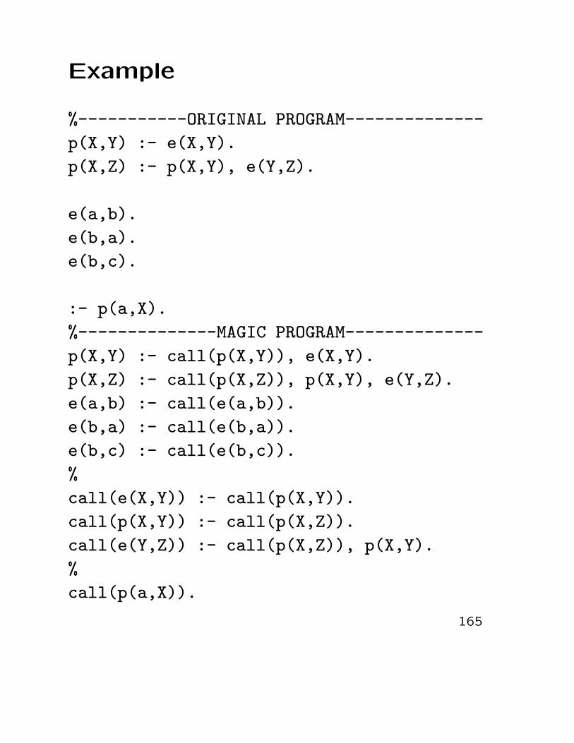
Example

%-----------ORIGINAL PROGRAM--------------

p(X,Y) :- e(X,Y).

p(X,Z) :- p(X,Y), e(Y,Z).

e(a,b).

e(b,a).

e(b,c).

:- p(a,X).

%--------------MAGIC PROGRAM--------------

p(X,Y) :- call(p(X,Y)), e(X,Y).

p(X,Z) :- call(p(X,Z)), p(X,Y), e(Y,Z).

e(a,b) :- call(e(a,b)).

e(b,a) :- call(e(b,a)).

e(b,c) :- call(e(b,c)).

%

call(e(X,Y)) :- call(p(X,Y)).

call(p(X,Y)) :- call(p(X,Z)).

call(e(Y,Z)) :- call(p(X,Z)), p(X,Y).

%

call(p(a,X)).

165

Bottom-up with Magic Templates

• Advantages:

– Termination;

– Re-use of results;

– Goal-directed;

• Disadvantages:

– Sometimes slower than Prolog (when

Prolog terminates);

166

Logic programming with Equations

• What is equality?

• E-unification.

• Logic programs with Equations

• SLDE-resolution

167

What is equality?

We sometimes want to express that two

terms should be interpreted as the same

object.

Example

Let Γ be:

person(X)← female(X).female(queen).silvia

.= queen.

Then Γ |= person(silvia).

168

Equations

An equation is an atom s.= t where s and t

are terms.

The predicate.= is always interpreted as the

identity relation.

That is, � |=σ s.= t iff σ�(s) = σ�(t).

Example

X + 0.= X.

X + s(Y ).= s(X + Y ).

1.= s(0).

2.= 1 + 1.

3.= 2 + 1....

169

Equality theory

E � s.= t: “s

.= t is derived from E”

{. . . , s .= t, . . .} � s

.= t

E � s.= s

E � s.= t

E � sσ.= tσ

E � s.= t

E � t.= s

E � r.= s E � s

.= t

E � r.= t

E � s1.= t1 · · · E � sn

.= tn

E � f(s1, . . . , sn).= f(t1, . . . , tn)

***

s ≡E t iff E � s.= t

170

Theorem

The relation ≡E is an equality relation.

Theorem

E |= s.= t iff s ≡E t (iff E � s

.= t) .

E-unification

Two terms s and t are E-unifiable iff sθ ≡E tθ.

The substitution θ is called an E-unifier.

171

Problem

• E-unification is undecidable;

• In general there is no single “most general

unifier” but only “complete sets of

E-unifiers”;

• This set may be infinite.

Unification. . .

. . . can be carried out using e.g. narrowing.

172

Logic programs with Equations

Programs consist of two components

• A set of definite clauses that do not

include the predicate symbol.=/2;

• A set of equations;

173

Observation

Herbrand interpretations are uninteresting!

Patch

Consider interpretations whose domain

consists of sets (equivalence classes) of

ground terms.

Every equivalence class consists of

“equivalent term”.

Interpretations with domain UP/ ≡E are of

special interest.

174

Let � be an interpretation where |�| = UP/≡E:

That is, s = {t ∈ UP | E � s.= t}.

Theorem

� |= s.= t iff s = t

iff s ≡E tiff E |= s

.= t

NB: Herbrand interpretations as a special

case!

175

The Least Model

Every program P, E has a least model MP,E:

P, E |= p(t1, . . . , tn) iff p(t1, . . . , tn) ∈MP,E

Fixed point semantics

TP,E(x) := {A | A← B1, . . . , Bn ∈ ground(P)∧B1, . . . , Bn ∈ x}

176

SLDE-Resolution

Given a goal

← A1, . . . , Ai−1, Ai, Ai+1, . . . , An

with selected literal Ai. If

• H ← B1, . . . , Bm is a renamed programclause

• H and Ai have a non-empty set Θ ofE-unifiers

• θ ∈ Θ

then

← (A1, . . . , Ai−1, B1, . . . , Bm, Ai+1, . . . , An)θ

is a new goal.

177

Theorem [Soundness]

If ← A1, . . . , An has a computed answer

substitution θ then P, E |= ∀(A1 ∧ · · · ∧An)θ.

Theorem [Completeness]

Similar to SLD-resolution.

178

Transparencies for the course TDDA41 Logic Programming ...

Documents

Transcript of Transparencies for the course TDDA41 Logic Programming ...