Transmission usage cost and loss allocation using AP and MP … · Transmission usage cost and loss...
53
AP Method ( Proportionate Tracing) Perturbation Analysis HVDC Line cost allocation Loss Allocation Loss Allocation Transmission usage cost and loss allocation using AP and MP-AP Method S. A. Soman Department of Electrical Engineering Indian Institute of Technology Bombay December 14, 2010
Transcript of Transmission usage cost and loss allocation using AP and MP … · Transmission usage cost and loss...

AP Method ( Proportionate Tracing) Perturbation Analysis HVDC Line cost allocation Loss Allocation Loss Allocation
Transmission usage cost and loss allocationusing AP and MP-AP Method
S. A. Soman
Department of Electrical EngineeringIndian Institute of Technology Bombay
December 14, 2010

AP Method ( Proportionate Tracing) Perturbation Analysis HVDC Line cost allocation Loss Allocation Loss Allocation
Outline
AP Method ( Proportionate Tracing)
Perturbation Analysis
HVDC Line cost allocation
Loss Allocation
Loss Allocation
AP Method ( Proportionate Tracing) Perturbation Analysis HVDC Line cost allocation Loss Allocation Loss Allocation
1
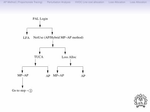
PAL Login
LFA
TUCA Loss Alloc
APAP MP−APMP−AP
Go to step −
NetUse (AP/Hybrid MP−AP method)
AP Method ( Proportionate Tracing) Perturbation Analysis HVDC Line cost allocation Loss Allocation Loss Allocation
2.1
1
2
3
2.2
3.5
3.4
3.3
3.2
3.6
3.7
3.8
3.9
3.1
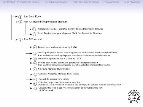
Run Load FLow
Run AP method (Proportionate Tracing)
Run MP method
Perturb each load one at a time by 1 MW
Perturb each load to absorb this generation − marginal losses in
Generation Tracing − compute dispersed Slack Bus Factors for Load
Load Tracing −compute dispersed Slack Bus Factors for Generator
Specify paticipation factors for each generator to absorb this l oad + marginal losses
Calculate Marginal FLow Matrix
Calculate Weighted Marginal Flow Matrix
Neglect the counter flow values
Perturb each generator one at a time by 1 MW
Calculate usage cost allocation for each line
Calculate the total usage cost for each entity and determine the PoC of AC network
Normalize each column of the matrix and multiply the column with the line usage cost
Run load flow modelling dispersed slack bus calculate marginal flow vector.
Run load flow modelling dispersed slack bus calculate marginal flow vector.
AP Method ( Proportionate Tracing) Perturbation Analysis HVDC Line cost allocation Loss Allocation Loss Allocation
4
4.2
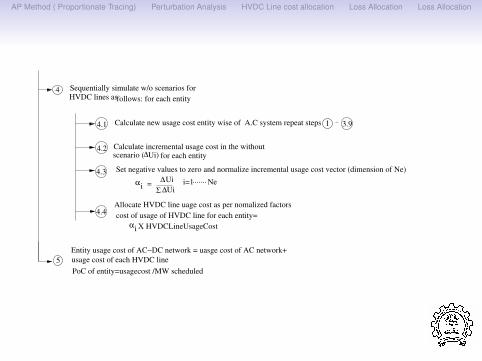
∆Ui
Σ ∆Uiαi =
4.3
αi X HVDCLineUsageCost
4.4
4.1 1 3.9
5
Sequentially simulate w/o scenarios for
scenario ( Ui)∆
Allocate HVDC line uage cost as per nomalized factors
cost of usage of HVDC line for each entity=
HVDC lines as follows: for each entity
Calculate incremental usage cost in the without for each entity
Calculate new usage cost entity wise of A.C system repeat steps
Set negative values to zero and normalize incremental usage cost vector (dimension of Ne)
i=1 Ne.......
Entity usage cost of AC−DC network = uasge cost of AC network+
usage cost of each HVDC line
PoC of entity=usagecost /MW scheduled

AP Method ( Proportionate Tracing) Perturbation Analysis HVDC Line cost allocation Loss Allocation Loss Allocation
1 2Repeat steps and
3
3.5
3.4
3.3
3.2
3.6
3.1
3.7
Run Loss Allocation
Run MP method
Perturb each load one at a time by 1 MW
Perturb each load to absorb this generation − marginal losses in
Specify paticipation factors for each generator to absorb this l oad + marginal losses
Perturb each generator one at a time by 1 MW
Run Load flow modelling dispersed slack bus and calculate the change in the system loss (kgi)
Run Load flow modelling dispersed slack bus and calculate the change in the system loss (kli)
Calculate a vector (V) by Weighting kgi and kli by the respective mw scheduled
Calculate loss allocation factor of entity i (LAFi) = Vi/ VΣ
Loss allocation of entity i = LAFi X systemloss

AP Method ( Proportionate Tracing) Perturbation Analysis HVDC Line cost allocation Loss Allocation Loss Allocation
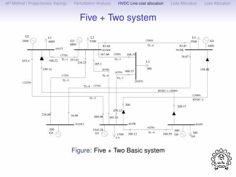
Five + Two system
G3 G4
G6G1G5
G2 L1 L2 L4
L6L5
3400 46004800
5300 3500
300600200 3343.28
1700
L3
300199.14
216.22384.96
167.525 168.191
82.673 82.808
16.67
200.17200
16.66216.66
468.19
395.17
101UT201WR 301DK
202ST1
501PU401PR302ST2
99.532 100
TL−2
HVDC−1
TL−1
(3750)
(12250)
TL−3
(2500)
TL−4
(7000)
TL−5
(1250) TL−6
(8750)
TL−7
(6250)
TL−8 (3750)
(6250)
TL−9
(30000)
HVDC−2
(15000)
199.48
3400
478.97
351.391347.942
668.748
653.098
Figure: Five + Two Basic system

AP Method ( Proportionate Tracing) Perturbation Analysis HVDC Line cost allocation Loss Allocation Loss Allocation
Generation TracingStarts from the pure source (501PU)Delete the pure source node, model its contributions to thereceipent nodes with generator tags
G3 G4
G1G5
G2 L1 L2 L4
L5
3400 46004800
5300 3500
200 3343.28
1700
L3
300
652.96 347.85 351.29216.36
384.88
167.46 168.12
82.68 82.81
16.67
200
478.89668.616.66216.66
468.11
395.09
101UT201WR 301DK
202ST1
401PR302ST2
TL−2
HVDC−1
TL−1
(3750)
(12250)
TL−3
(2500)
TL−4
(7000)
TL−5
(1250) TL−6
(8750)
TL−7
(6250)
TL−8 (3750)
(30000)
HVDC−2
(15000)
G6
199.14
199.48
3400
G6
99.36
Figure: Elimination of node 501PU

AP Method ( Proportionate Tracing) Perturbation Analysis HVDC Line cost allocation Loss Allocation Loss Allocation
G3 G4
G2 L1 L2 L4
3400 46004800
5300 3500
L3
300
347.85 351.29
167.46 168.12
82.68 82.81
16.67
16.66216.66
101UT201WR 301DK
202ST1
302ST2
TL−1
(3750)
TL−3
(2500)
TL−4
(7000)
(1250) G6
G1 G6
13.51
454.61
G1
G1
G5
(3750)TL−8
TL−5
193.72 5.76
3400
216.36 373.77 11.11
G6G1
200
G6
218.03635.02
Figure: Elimination of node 401PR

AP Method ( Proportionate Tracing) Perturbation Analysis HVDC Line cost allocation Loss Allocation Loss Allocation
G3
G2 L13400 4600
4800
L3
300
347.85 351.29216.36
167.46 168.12
216.66
101UT201WR
302ST2
TL−1
(3750)
TL−3
(2500)
TL−5
(1250)
G6
218.03
G6
13.51
454.61
G1
G1
634.12 G4
11.28
78.09
G1
0.89
G5
200
G415.74
G6
0.03
202ST1
5300
L2 G1 G6
378.22
Figure: Elimination of node 301DK
AP Method ( Proportionate Tracing) Perturbation Analysis HVDC Line cost allocation Loss Allocation Loss Allocation
G3
G2 L13400 4600
4800
347.85 351.29216.36
216.66
101UT201WR
302ST2
TL−1
(3750)
TL−5
(1250)
G6
218.03
G1
634.12 G4
16.11
78.09
G1
0.89
G5
200
G415.74
G6
0.03
L2
5300 540.85
G6G1
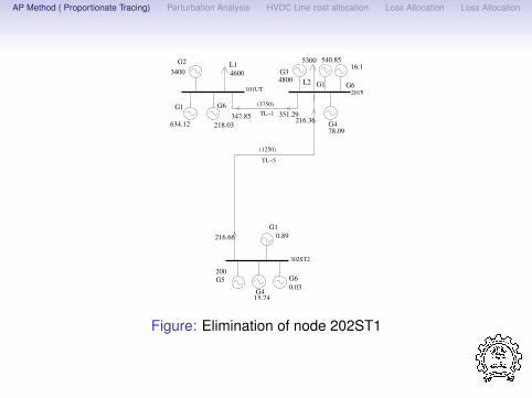
Figure: Elimination of node 202ST1

AP Method ( Proportionate Tracing) Perturbation Analysis HVDC Line cost allocation Loss Allocation Loss Allocation
G3
G2 L13400 4600
4800
347.85 351.29
101UT
TL−1
(3750)G6
218.03
G1
634.12 G4
541.74
93.81G5199.72
5300
L2 G1 G6
16.14
201WR
Figure: Elimination of node 302ST2

AP Method ( Proportionate Tracing) Perturbation Analysis HVDC Line cost allocation Loss Allocation Loss Allocation
G1
667.46
3400
G2 4600
L1 G6
219.02
G5
12.29
G3
295.45
G4
5.77
101UT
Figure: Elimination of node 201WR
AP Method ( Proportionate Tracing) Perturbation Analysis HVDC Line cost allocation Loss Allocation Loss Allocation
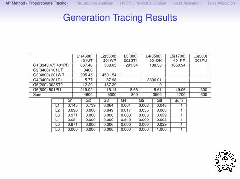
Generation Tracing Results
L1(4600) L2(5300) L3(300) L4(3500) L5(1700) L6(300)101UT 201WR 202ST1 301DK 401PR 501PU
G1(3343.47) 401PR 667.46 508.05 291.34 188.38 1650.94G2(3400) 101UT 3400G3(4800) 201WR 295.45 4501.54G4(3400) 301Dk 5.77 87.98 3306.01G5(200) 302ST2 12.29 187.29 0G6(600) 501PU 219.02 15.14 8.66 5.61 49.06 300Sum 4600 5300 300 3500 1700 300
G1 G2 G3 G4 G5 G6 SumL1 0.145 0.739 0.064 0.001 0.003 0.048 1L2 0.096 0.000 0.849 0.017 0.035 0.003 1L3 0.971 0.000 0.000 0.000 0.000 0.029 1L4 0.054 0.000 0.000 0.945 0.000 0.002 1L5 0.971 0.000 0.000 0.000 0.000 0.029 1L6 0.000 0.000 0.000 0.000 0.000 1.000 1

AP Method ( Proportionate Tracing) Perturbation Analysis HVDC Line cost allocation Loss Allocation Loss Allocation
Five + Two system
G3 G4
G6G1G5
G2 L1 L2 L4
L6L5
3400 46004800
5300 3500
300600200 3343.28
1700
L3
300199.14
216.22384.96
167.525 168.191
82.673 82.808
16.67
200.17200
16.66216.66
468.19
395.17
101UT201WR 301DK
202ST1
501PU401PR302ST2
99.532 100
TL−2
HVDC−1
TL−1
(3750)
(12250)
TL−3
(2500)
TL−4
(7000)
TL−5
(1250) TL−6
(8750)
TL−7
(6250)
TL−8 (3750)
(6250)
TL−9
(30000)
HVDC−2
(15000)
199.48
3400
478.97
351.391347.942
668.748
653.098
Figure: Five + Two Basic system
AP Method ( Proportionate Tracing) Perturbation Analysis HVDC Line cost allocation Loss Allocation Loss Allocation
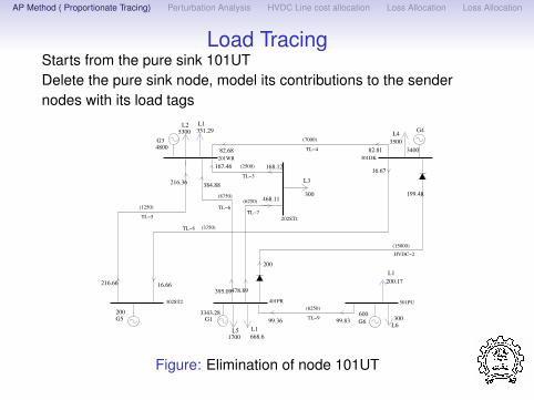
Load TracingStarts from the pure sink 101UTDelete the pure sink node, model its contributions to the sendernodes with its load tags
G3
G6G1G5
L4
L6
48003500
300600200 3343.28
L3
300
216.36384.88
167.46 168.12
82.68 82.81
16.67
200
16.66216.66
468.11
201WR 301DK
202ST1
501PU401PR302ST2
99.36 99.83
TL−3
(2500)
TL−4
(7000)
TL−5
(1250) TL−6
(8750)
TL−7
(6250)
TL−8 (3750)
(6250)
TL−9
HVDC−2
(15000)
L51700
L1
668.6
L2
5300 351.29
L1
L1
200.17
G4
199.48
3400
478.89395.09
Figure: Elimination of node 101UT

AP Method ( Proportionate Tracing) Perturbation Analysis HVDC Line cost allocation Loss Allocation Loss Allocation
G4
G6G1G5L6
600200 3343.28
L2
157.67
200
468.11
202ST1
401PR302ST2
99.36 99.83
TL−7
(6250)
TL−8 (3750)
(6250)
TL−9
HVDC−2
(15000)
L5 L1
695.16
L1
200.17
1700
370.49
L2
L1
L3
10.45
300
L4
3500
L2
77.66
L1
5.15
199.48
3400
300
501PU
203.1913.47
16.66L1 L2
16.67
301DK
478.89
Figure: Elimination of node 201WR

AP Method ( Proportionate Tracing) Perturbation Analysis HVDC Line cost allocation Loss Allocation Loss Allocation
G4
G6G1L6
3400
3006003343.28
L2
157.67 199.48
200
468.11
301DK
202ST1
501PU401PR
99.36 99.83
TL−7
(6250)
(6250)
TL−9
HVDC−2
(15000)
L5 L1
695.16
L1
200.17
1700
370.49
L2
L1
L3
10.45
300
L4
3500
L2
93.29
L1
6.19
478.89
Figure: Elimination of node 302ST2

AP Method ( Proportionate Tracing) Perturbation Analysis HVDC Line cost allocation Loss Allocation Loss Allocation
G6G1L6
3006003343.28
200
301DK
501PU401PR
99.36 99.83
(6250)
TL−9
HVDC−2
(15000)
L5 L1
703.85
L1
200.17
1700
L4
3500
L2
93.29
L1
6.19
531.79
L2
L3
306.9
3400
G4
199.48
Figure: Elimination of node 202ST1

AP Method ( Proportionate Tracing) Perturbation Analysis HVDC Line cost allocation Loss Allocation Loss Allocation
G6G1L6
6003343.28
401PR
99.36 99.83
(6250)
TL−9
L5 L1
704.191700
536.96
L2 200.17
L1
306.9
L3
194.47
L4
501PU
300
Figure: Elimination of node 301DK

AP Method ( Proportionate Tracing) Perturbation Analysis HVDC Line cost allocation Loss Allocation Loss Allocation
600
G6
L6
300
L2
15.57
L3
8.9
220.59
L5
49.3
5.64
L4 L1
501PU
Figure: Elimination of node 401PR

AP Method ( Proportionate Tracing) Perturbation Analysis HVDC Line cost allocation Loss Allocation Loss Allocation
Load tracing Results
G1(3343.47) G2(3400) G3(4800) G4(3400) G5(200) G6(600)401PR 101UT 201WR 301DK 302ST2 501PU
L1(4600) 101UT 683.94 3400 298.37 5.85 12.43 220.59L2(5300) 201WR 521.48 4501.63 88.12 187.57 15.57L3(300) 202ST1 298.04 8.9L4(3500) 301DK 188.88 3306.03 5.64L5(1700) 401PR 1650.94 49.3L6(300) 501PU 300
3343.47 3400 4800 3400 200 600L1 L2 L3 L4 L5 L6 Sum
G1 0.205 0.156 0.089 0.056 0.494 0.000 1G2 1.000 0.000 0.000 0.000 0.000 0.000 1G3 0.062 0.938 0.000 0.000 0.000 0.000 1G4 0.002 0.026 0.000 0.972 0.000 0.000 1G5 0.062 0.938 0.000 0.000 0.000 0.000 1G6 0.368 0.026 0.015 0.009 0.082 0.500 1

AP Method ( Proportionate Tracing) Perturbation Analysis HVDC Line cost allocation Loss Allocation Loss Allocation
Perturbation with G1L1 L2 L3 L4 L5 L6
G1 0.202 0.154 0.088 0.057 0.499 0.000
G3 G4
G6G5
G2 L1 L2 L4
3400 46004800
5300 3500
300600200 3343.28
1700
L3
300
652.96
199.14
347.85 351.29
384.88
167.46 168.12
82.42
16.67
200.17200
668.616.66216.66395.09
101UT201WR 301DK
202ST1
501PU401PR302ST2
99.36 99.83
TL−2
HVDC−1
TL−1
(3750)
(12250)
TL−3
(2500)
TL−4
(7000)
TL−5
(1250) TL−6
(8750)
TL−7
(6250)
TL−8 (3750)
(6250)
TL−9
(30000)
HVDC−2
(15000)
199.48
3400
G1+10.0
+2.02 +1.54
+0.88
+0.57
L5+4.99 L6
0.00
216.36351.49
670.61
168.97
82.81
82.56
216.35396.7
478.89
480.73
99.83
348.04654.87
168.3
82.68
215.91386.41 468.11
469.87
16.36
16.35
99.36
Figure: Perturbation of G1
Marginal Flow Vector:
Entity Psch TL-1 TL-2 TL-3 TL-4 TL-5 TL-6 TL-7 TL-8 TL-9G1 3343.37 0.018 0.196 0.083 -0.031 -0.025 0.157 0.180 -0.025 0.000

AP Method ( Proportionate Tracing) Perturbation Analysis HVDC Line cost allocation Loss Allocation Loss Allocation
Perturbation with G2L1 L2 L3 L4 L5 L6
G2 1.000 0.000 0.000 0.000 0.000 0.000
G3 G4
G6G5
G2 L1 L2 L4
3400 46004800
5300 3500
300600200 3343.28
1700
L3
300
652.96
199.14
347.85 351.29
384.88
167.46 168.1216.67
200.17200
668.616.66216.66395.09
101UT201WR 301DK
202ST1
501PU401PR302ST2
99.36 99.83
TL−2
HVDC−1
TL−1
(3750)
(12250)
TL−3
(2500)
TL−4
(7000)
TL−5
(1250) TL−6
(8750)
TL−7
(6250)
TL−8 (3750)
(6250)
TL−9
(30000)
HVDC−2
(15000)
199.48
3400
G1
+10.0
0.0
0.0
L50.0 L6
0.00
216.36
668.6
82.81
216.66395.09
478.89
99.83
82.68
468.11
99.36
+10.0 0.0
168.12167.46
82.8182.68
468.11
384.88
16.67
216.36
351.29347.85652.96
478.89
16.66
Figure: Perturbation of G2
Marginal Flow Vector:
Entity Psch TL-1 TL-2 TL-3 TL-4 TL-5 TL-6 TL-7 TL-8 TL-9G2 3400 0.000 0.000 0.000 0.000 0.000 0.000 0.000 0.000 0.000

AP Method ( Proportionate Tracing) Perturbation Analysis HVDC Line cost allocation Loss Allocation Loss Allocation
Perturbation with G3L1 L2 L3 L4 L5 L6
G3 0.062 0.938 0.000 0.000 0.000 0.000
G3 G4
G6G5
G2 L1 L2 L4
3400 46004800
5300 3500
300600200 3343.28
1700
L3
300
652.96
199.14
347.85 351.29
384.88
167.46 168.12
82.74
16.67
200.17200
668.616.66216.66395.09
101UT201WR 301DK
202ST1
501PU401PR302ST2
99.36 99.83
TL−2
HVDC−1
TL−1
(3750)
(12250)
TL−3
(2500)
TL−4
(7000)
TL−5
(1250) TL−6
(8750)
TL−7
(6250)
TL−8 (3750)
(6250)
TL−9
(30000)
HVDC−2
(15000)
199.48
3400
G1
+0.62
0.0
0.0
L50.0 L6
0.00
216.36
668.81
82.81
82.87
216.6395.06
478.89
478.86
99.83
653.15
82.68
216.17384.85 468.11
468.08
16.61
16.6
99.36
+9.38
351.79168.08167.41
+10.0
348.33
Figure: Perturbation of G3
Marginal Flow Vector:
Entity Psch TL-1 TL-2 TL-3 TL-4 TL-5 TL-6 TL-7 TL-8 TL-9G3 4800 0.048 0.016 -0.007 0.000 0.000 -0.007 -0.007 0.000 0.000
AP Method ( Proportionate Tracing) Perturbation Analysis HVDC Line cost allocation Loss Allocation Loss Allocation
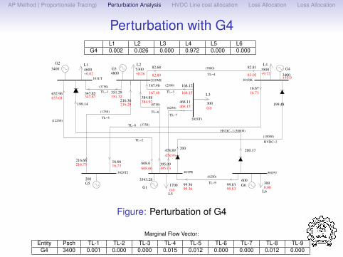
Perturbation with G4L1 L2 L3 L4 L5 L6
G4 0.002 0.026 0.000 0.972 0.000 0.000
G3 G4
G6G5
G2 L1 L2 L4
3400 46004800
5300 3500
300600200 3343.28
1700
L3
300
652.96
199.14
347.85 351.29
384.88
167.46 168.12
82.89
16.67
200.17200
668.616.66216.66395.09
101UT201WR 301DK
202ST1
501PU401PR302ST2
99.36 99.83
TL−2
HVDC−1
TL−1
(3750)
(12250)
TL−3
(2500)
TL−4
(7000)
TL−5
(1250) TL−6
(8750)
TL−7
(6250)
TL−8 (3750)
(6250)
TL−9
(30000)
HVDC−2
(15000)
199.48
3400
G1
+0.02
0.0
+9.72
L50.0 L6
0.00
216.36
668.66
82.81
83.02
216.73395.13
478.89
99.83
653.01
82.68
216.29384.92 468.11
468.15
16.73
16.73
99.36
351.32168.15167.48
347.87
+10.0+0.26
478.93
Figure: Perturbation of G4
Marginal Flow Vector:
Entity Psch TL-1 TL-2 TL-3 TL-4 TL-5 TL-6 TL-7 TL-8 TL-9G4 3400 0.001 0.000 0.000 0.015 0.012 0.000 0.000 0.012 0.000

AP Method ( Proportionate Tracing) Perturbation Analysis HVDC Line cost allocation Loss Allocation Loss Allocation
Perturbation with G5L1 L2 L3 L4 L5 L6
G5 0.062 0.938 0.000 0.000 0.000 0.000
G3 G4
G6
G2 L1 L2 L4
3400 46004800
5300 3500
300600200 3343.28
1700
L3
300
652.96
199.14
347.85 351.29
384.88
167.46 168.12
84.12
16.67
200.17200
668.616.66216.66395.09
101UT201WR 301DK
202ST1
501PU401PR302ST2
99.36 99.83
TL−2
HVDC−1
TL−1
(3750)
(12250)
TL−3
(2500)
TL−4
(7000)
TL−5
(1250) TL−6
(8750)
TL−7
(6250)
TL−8 (3750)
(6250)
TL−9
(30000)
HVDC−2
(15000)
199.48
3400
G1
+0.62
0.0
+9.72
L50.0 L6
0.00
216.36
668.82
82.81
84.26
225.22395.07
478.89
99.83
653.16
82.68
224.75384.87 468.11
468.09
15.23
15.22
99.36
351.78168.09167.43
348.32
+9.38
478.87
G5+10.0
Figure: Perturbation of G5
Marginal Flow Vector:
Entity Psch TL-1 TL-2 TL-3 TL-4 TL-5 TL-6 TL-7 TL-8 TL-9G5 200 0.047 0.017 -0.006 0.138 0.862 -0.006 -0.006 -0.138 0.000

AP Method ( Proportionate Tracing) Perturbation Analysis HVDC Line cost allocation Loss Allocation Loss Allocation
Perturbation with G6L1 L2 L3 L4 L5 L6
G6 0.367 0.025 0.014 0.009 0.082 0.502
G3 G4
G2 L1 L2 L4
3400 46004800
5300 3500
300600200 3343.28
1700
L3
300
652.96
199.14
347.85 351.29
384.88
167.46 168.12
82.68
16.67
200.17200
668.616.66216.66395.09
101UT201WR 301DK
202ST1
501PU401PR302ST2
99.36 99.83
TL−2
HVDC−1
TL−1
(3750)
(12250)
TL−3
(2500)
TL−4
(7000)
TL−5
(1250) TL−6
(8750)
TL−7
(6250)
TL−8 (3750)
(6250)
TL−9
(30000)
HVDC−2
(15000)
199.48
3400
G1
+3.67
+0.14
+0.09
L5+0.82 L6
+5.02
216.36
670.81
82.81
82.82
216.56396.25
478.89
104.83
655.06
82.68
216.12385.98 468.11
469.25
16.57
16.56
104.32
352.96169.1168.42
349.48
+0.25
480.08
G5+10.0G6
Figure: Perturbation of G6
Marginal Flow Vector:
Entity Psch TL-1 TL-2 TL-3 TL-4 TL-5 TL-6 TL-7 TL-8 TL-9G6 600 0.165 0.216 0.095 -0.005 -0.004 0.112 0.115 -0.004 0.500

AP Method ( Proportionate Tracing) Perturbation Analysis HVDC Line cost allocation Loss Allocation Loss Allocation
Perturbation with L1G1 G2 G3 G4 G5 G6
L1 0.148 0.736 0.065 0.001 0.003 0.048
3400 4600 5300
3001700
L3
300
652.96
199.14
384.88
16.67
200.17200
468.11
101UT201WR 301DK
202ST1
501PU401PR302ST2
99.36 99.83
TL−2
HVDC−1
TL−1
(3750)
(12250)
TL−3
(2500)
TL−4
(7000)
TL−5
(1250) TL−6
(8750)
TL−7
(6250)
TL−8 (3750)
(6250)
TL−9
(30000)
HVDC−2
(15000)
199.48
L4
35004800
L5G1
3343.28200
G5 G6
600
L6+0.48+0.03
G4
3400 +0.01
G2 L1
+7.36 +0.65
G3 L2
+1.48
+10
167.87 168.54
82.8882.75
468.54
351.29352.77
347.85349.30
216.36216.19654.18
385.32
167.46 168.12
82.68 82.81
16.61
395.55395.09
668.6669.88 479.34
478.89
100.3199.84
16.6616.61
216.66216.63
Figure: Perturbation of L1
Marginal Flow Vector:
Entity Psch TL-1 TL-2 TL-3 TL-4 TL-5 TL-6 TL-7 TL-8 TL-9L1 4600 0.147 0.123 0.039 0.001 0.003 0.042 0.041 0.000 0.048
AP Method ( Proportionate Tracing) Perturbation Analysis HVDC Line cost allocation Loss Allocation Loss Allocation
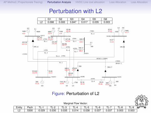
Perturbation with L2G1 G2 G3 G4 G5 G6
L2 0.098 0.000 0.847 0.017 0.035 0.003
3400 4600 5300
3001700
L3
300
652.96
199.14
384.88
16.67
200.17200
468.11
101UT201WR 301DK
202ST1
501PU401PR302ST2
99.36 99.83
TL−2
HVDC−1
TL−1
(3750)
(12250)
TL−3
(2500)
TL−4
(7000)
TL−5
(1250) TL−6
(8750)
TL−7
(6250)
TL−8 (3750)
(6250)
TL−9
(30000)
HVDC−2
(15000)
199.48
L4
35004800
L5G1
3343.28200
G5 G6
600
L6
G4
3400
G2 L1 G3 L2
351.29347.85
216.36
167.46 168.12
82.68 82.81
395.09
668.6 478.89
16.66216.66
+10
+0.98
+0.0 +8.47 +0.17
+0.35+0.03
351.02347.57
653.29
668.95
168.5167.83
83.0182.88
216.98
216.54
395.5
385.27
479.3
468.5
16.63
16.64
99.8699.39
Figure: Perturbation of L2
Marginal Flow Vector:
Entity Psch TL-1 TL-2 TL-3 TL-4 TL-5 TL-6 TL-7 TL-8 TL-9L2 5300 -0.029 0.030 0.035 0.014 0.038 0.037 0.037 0.003 0.003

AP Method ( Proportionate Tracing) Perturbation Analysis HVDC Line cost allocation Loss Allocation Loss Allocation
Perturbation with L3G1 G2 G3 G4 G5 G6
L3 0.971 0.000 0.000 0.000 0.000 0.029
3400 4600 5300
3001700
L3
300
652.96
199.14
384.88
16.67
200.17200
468.11
101UT201WR 301DK
202ST1
501PU401PR302ST2
99.36 99.83
TL−2
HVDC−1
TL−1
(3750)
(12250)
TL−3
(2500)
TL−4
(7000)
TL−5
(1250) TL−6
(8750)
TL−7
(6250)
TL−8 (3750)
(6250)
TL−9
(30000)
HVDC−2
(15000)
199.48
L4
35004800
L5G1
3343.28200
G5 G6
600
L6
G4
3400
G2 L1 G3 L2
351.29347.85
216.36
167.46 168.12
82.68 82.81
395.09
668.6 478.89
16.66216.66
+0.0
+10
+9.71+0.29
+0.0+0.0
+0.0
349.17345.77
670.85
655.1
163.39162.75
82.8782.74
216.6
216.17
395.87
387.52
484.43
473.39
16.61
16.6
99.65 100.12
Figure: Perturbation of L3
Marginal Flow Vector:
Entity Psch TL-1 TL-2 TL-3 TL-4 TL-5 TL-6 TL-7 TL-8 TL-9L3 300 -0.213 0.220 -0.476 0.000 0.000 0.274 0.550 0.000 0.029
AP Method ( Proportionate Tracing) Perturbation Analysis HVDC Line cost allocation Loss Allocation Loss Allocation
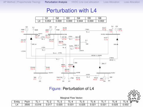
Perturbation with L4G1 G2 G3 G4 G5 G6
L4 0.054 0.000 0.000 0.944 0.000 0.002
3400 4600 5300
3001700
L3
300
652.96
199.14
384.88
16.67
200.17200
468.11
101UT201WR 301DK
202ST1
501PU401PR302ST2
99.36 99.83
TL−2
HVDC−1
TL−1
(3750)
(12250)
TL−3
(2500)
TL−4
(7000)
TL−5
(1250) TL−6
(8750)
TL−7
(6250)
TL−8 (3750)
(6250)
TL−9
(30000)
HVDC−2
(15000)
199.48
L4
35004800
L5G1
3343.28200
G5 G6
600
L6
G4
3400
G2 L1 G3 L2
351.29347.85
216.36
167.46 168.12
82.68 82.81
395.09
668.6 478.89
16.66216.66
+0.0 +0.0
+0.0
+10
+0.54
+9.44
+0.02
351.14347.7
668.82
653.16
167.68
82.5682.43
216.36
215.92
395.34
385.12
479.14
468.34
16.36
16.36
99.8599.38
168.34
Figure: Perturbation of L4
Marginal Flow Vector:
Entity Psch TL-1 TL-2 TL-3 TL-4 TL-5 TL-6 TL-7 TL-8 TL-9L4 3500 -0.016 0.017 0.020 -0.031 -0.025 0.021 0.021 -0.025 0.002

AP Method ( Proportionate Tracing) Perturbation Analysis HVDC Line cost allocation Loss Allocation Loss Allocation
Perturbation with L5G1 G2 G3 G4 G5 G6
L5 0.971 0.000 0.000 0.000 0.000 0.029
3400 4600 5300
3001700
L3
300
652.96
199.14
384.88
16.67
200.17200
468.11
101UT201WR 301DK
202ST1
501PU401PR302ST2
99.36 99.83
TL−2
HVDC−1
TL−1
(3750)
(12250)
TL−3
(2500)
TL−4
(7000)
TL−5
(1250) TL−6
(8750)
TL−7
(6250)
TL−8 (3750)
(6250)
TL−9
(30000)
HVDC−2
(15000)
199.48
L4
35004800
L5G1
3343.28200
G5 G6
600
L6
G4
3400
G2 L1 G3 L2
351.29347.85
216.36
167.46 168.12
82.68 82.81
395.09
668.6 478.89
16.66216.66
+0.0 +0.0
+0.0 +10+9.71 +0.29
+0.0
351.31347.86
668.65
653.01
168.15167.48
82.8782.74
216.6
216.17
395.13
384.92
478.93
468.15
16.61
16.6
100.1299.65
Figure: Perturbation of L5
Marginal Flow Vector:
Entity Psch TL-1 TL-2 TL-3 TL-4 TL-5 TL-6 TL-7 TL-8 TL-9L5 1700 0.000 0.000 0.000 0.000 0.000 0.000 0.000 0.000 0.029

AP Method ( Proportionate Tracing) Perturbation Analysis HVDC Line cost allocation Loss Allocation Loss Allocation
Perturbation with L6G1 G2 G3 G4 G5 G6
L6 0.000 0.000 0.000 0.000 0.000 1.000
3400 4600 5300
3001700
L3
300
652.96
199.14
384.88
16.67
200.17200
468.11
101UT201WR 301DK
202ST1
501PU401PR302ST2
99.36 99.83
TL−2
HVDC−1
TL−1
(3750)
(12250)
TL−3
(2500)
TL−4
(7000)
TL−5
(1250) TL−6
(8750)
TL−7
(6250)
TL−8 (3750)
(6250)
TL−9
(30000)
HVDC−2
(15000)
199.48
L4
35004800
L5G1
3343.28200
G5 G6
600
L6
G4
3400
G2 L1 G3 L2
351.29347.85
216.36
167.46 168.12
82.68 82.81
395.09
668.6 478.89
16.66216.66
+0.0 +0.0
+0.0
+0.0
347.85
168.12
82.81
216.66
395.09
478.89
16.61
16.66
+10+10+0.0 99.8399.36
652.96
351.29
216.36384.88
167.46
468.11
668.6
82.68
Figure: Perturbation of L6
Marginal Flow Vector:
Entity Psch TL-1 TL-2 TL-3 TL-4 TL-5 TL-6 TL-7 TL-8 TL-9L6 300 0.000 0.000 0.000 0.000 0.000 0.000 0.000 0.000 0.000

AP Method ( Proportionate Tracing) Perturbation Analysis HVDC Line cost allocation Loss Allocation Loss Allocation
Marginal Flows
Entity Psch TL-1 TL-2 TL-3 TL-4 TL-5 TL-6 TL-7 TL-8 TL-9G1 3343.37 0.018 0.196 0.083 -0.031 -0.025 0.157 0.180 -0.025 0.000G2 3400 0.000 0.000 0.000 0.000 0.000 0.000 0.000 0.000 0.000G3 4800 0.048 0.016 -0.007 0.000 0.000 -0.007 -0.007 0.000 0.000G4 3400 0.001 0.000 0.000 0.015 0.012 0.000 0.000 0.012 0.000G5 200 0.047 0.017 -0.006 0.138 0.862 -0.006 -0.006 -0.138 0.000G6 600 0.165 0.216 0.095 -0.005 -0.004 0.112 0.115 -0.004 0.500L1 4600 0.147 0.123 0.039 0.001 0.003 0.042 0.041 0.000 0.048L2 5300 -0.029 0.030 0.035 0.014 0.038 0.037 0.037 0.003 0.003L3 300 -0.213 0.220 -0.476 0.000 0.000 0.274 0.550 0.000 0.029L4 3500 -0.016 0.017 0.020 -0.031 -0.025 0.021 0.021 -0.025 0.002L5 1700 0.000 0.000 0.000 0.000 0.000 0.000 0.000 0.000 0.029L6 300 0.000 0.000 0.000 0.000 0.000 0.000 0.000 0.000 0.000
AP Method ( Proportionate Tracing) Perturbation Analysis HVDC Line cost allocation Loss Allocation Loss Allocation
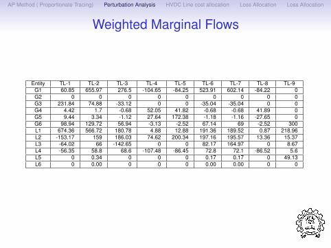
Weighted Marginal Flows
Entity TL-1 TL-2 TL-3 TL-4 TL-5 TL-6 TL-7 TL-8 TL-9G1 60.85 655.97 276.5 -104.65 -84.25 523.91 602.14 -84.22 0G2 0 0 0 0 0 0 0 0 0G3 231.84 74.88 -33.12 0 0 -35.04 -35.04 0 0G4 4.42 1.7 -0.68 52.05 41.82 -0.68 -0.68 41.89 0G5 9.44 3.34 -1.12 27.64 172.38 -1.18 -1.16 -27.65 0G6 98.94 129.72 56.94 -3.13 -2.52 67.14 69 -2.52 300L1 674.36 566.72 180.78 4.88 12.88 191.36 189.52 0.87 218.96L2 -153.17 159 186.03 74.62 200.34 197.16 195.57 13.36 15.37L3 -64.02 66 -142.65 0 0 82.17 164.97 0 8.67L4 -56.35 58.8 68.6 -107.48 -86.45 72.8 72.1 -86.52 5.6L5 0 0.34 0 0 0 0.17 0.17 0 49.13L6 0 0.00 0 0 0 0.00 0.00 0 0

AP Method ( Proportionate Tracing) Perturbation Analysis HVDC Line cost allocation Loss Allocation Loss Allocation
Neglect Negative Marginal Flow
Entity TL-1 TL-2 TL-3 TL-4 TL-5 TL-6 TL-7 TL-8 TL-9G1 60.85 655.97 276.5 0 0 523.91 602.14 0 0G2 0 0 0 0 0 0 0 0 0G3 231.84 74.88 0 0 0 0 0 0 0G4 4.42 1.7 0 52.05 41.82 0 0 41.89 0G5 9.44 3.34 0 27.64 172.38 0 0 0 0G6 98.94 129.72 56.94 0 0 67.14 69 0 300L1 674.36 566.72 180.78 4.88 12.88 191.36 189.52 0.87 218.96L2 0 159 186.03 74.62 200.34 197.16 195.57 13.36 15.37L3 0 66 0 0 0 82.17 164.97 0 8.67L4 0 58.8 68.6 0 0 72.8 72.1 0 5.6L5 0 0.34 0 0 0 0.17 0.17 0 49.13L6 0 0.00 0 0 0 0.00 0.00 0 0

AP Method ( Proportionate Tracing) Perturbation Analysis HVDC Line cost allocation Loss Allocation Loss Allocation
Normalization over the line
Entity TL-1 TL-2 TL-3 TL-4 TL-5 TL-6 TL-7 TL-8 TL-9G1 0.06 0.38 0.36 0.00 0.00 0.46 0.47 0.00 0.00G2 0.00 0.00 0.00 0.00 0.00 0.00 0.00 0.00 0.00G3 0.21 0.04 0.00 0.00 0.00 0.00 0.00 0.00 0.00G4 0.00 0.00 0.00 0.33 0.10 0.00 0.00 0.75 0.00G5 0.01 0.00 0.00 0.17 0.40 0.00 0.00 0.00 0.00G6 0.09 0.08 0.07 0.00 0.00 0.06 0.05 0.00 0.50L1 0.62 0.33 0.24 0.03 0.03 0.17 0.15 0.02 0.37L2 0.00 0.09 0.24 0.47 0.47 0.17 0.15 0.24 0.03L3 0.00 0.04 0.00 0.00 0.00 0.07 0.13 0.00 0.01L4 0.00 0.03 0.09 0.00 0.00 0.06 0.06 0.00 0.01L5 0.00 0.00 0.00 0.00 0.00 0.00 0.00 0.00 0.08L6 0.00 0.00 0.00 0.00 0.00 0.00 0.00 0.00 0.00
LineCost 3750 12250 2500 7000 1250 8750 6250 3750 6250

AP Method ( Proportionate Tracing) Perturbation Analysis HVDC Line cost allocation Loss Allocation Loss Allocation
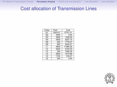
Cost allocation of Transmission Lines
Entity TL-1 TL-2 TL-3 TL-4 TL-5 TL-6 TL-7 TL-8 TL-9G1 211.31 4681.32 899.06 0.00 0.00 4039.86 2909.45 0.00 0.00G2 0.00 0.00 0.00 0.00 0.00 0.00 0.00 0.00 0.00G3 805.11 534.38 0.00 0.00 0.00 0.00 0.00 0.00 0.00G4 15.35 12.13 0.00 2288.84 122.30 0.00 0.00 2799.10 0.00G5 32.78 23.84 0.00 1215.52 504.13 0.00 0.00 0.00 0.00G6 343.59 925.75 185.15 0.00 0.00 517.72 333.40 0.00 3136.87L1 2341.85 4044.39 587.83 214.40 37.67 1475.59 915.73 58.40 2289.50L2 0.00 1134.70 604.90 3281.25 585.90 1520.31 944.96 892.49 160.71L3 0.00 471.01 0.00 0.00 0.00 633.62 797.11 0.00 90.66L4 0.00 419.63 223.06 0.00 0.00 561.36 348.38 0.00 58.55L5 0.00 2.43 0.00 0.00 0.00 1.31 0.82 0.00 513.71L6 0.00 0.0 0.00 0.00 0.00 0.0 0.0 0.00 0.00
AP Method ( Proportionate Tracing) Perturbation Analysis HVDC Line cost allocation Loss Allocation Loss Allocation
Cost allocation of Transmission Lines
Entity Psch CostG1 3343.47 12741.01G2 3400 0.00G3 4800 1339.49G4 3400 5237.72G5 200 1776.27G6 600 5442.47L1 4600 11965.36L2 5300 9125.23L3 300 1992.39L4 3500 1610.98L5 1700 518.27L6 300 0.00
AP Method ( Proportionate Tracing) Perturbation Analysis HVDC Line cost allocation Loss Allocation Loss Allocation
Five + Two system
G3 G4
G6G1G5
G2 L1 L2 L4
L6L5
3400 46004800
5300 3500
300600200 3343.28
1700
L3
300
653.4
199.14
348.22 351.67216.23
385.1
167.66 168.33
82.68 82.81
16.67
200.17200
669.0616.66216.66
468.33
395.33
101UT201WR 301DK
202ST1
501PU401PR302ST2
100.12 100.59
TL−2
HVDC−1
TL−1
(3750)
(12250)
TL−3
(2500)
TL−4
(7000)
TL−5
(1250) TL−6
(8750)
TL−7
(6250)
TL−8 (3750)
(6250)
TL−9
(30000)
HVDC−2
(15000)
199.48
3400
479.12
Figure: Five + Two Basic system
AP Method ( Proportionate Tracing) Perturbation Analysis HVDC Line cost allocation Loss Allocation Loss Allocation
G3 G4
G6G1G5
G2 L1 L2 L4
L6L5
3400 46004800
5300 3500
300600200 3343.28
1700
L3
300
756.84 443.16 448.78216.23
433.92
219.96 217.04
82.68 82.81
16.67
200
778.2716.66216.66
517.04
447.02
101UT201WR 301DK
202ST1
501PU401PR302ST2
295.81 300
TL−2
TL−1
(3750)
(12250)
TL−3
(2500)
TL−4
(7000)
TL−5
(1250) TL−6
(8750)
TL−7
(6250)
TL−8 (3750)
(6250)
TL−9
HVDC−2
(15000)
199.48
3400
530.31
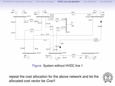
Figure: System without HVDC line 1
repeat the cost allocation for the above network and let theallocated cost vector be Cost1

AP Method ( Proportionate Tracing) Perturbation Analysis HVDC Line cost allocation Loss Allocation Loss Allocation
G3 G4
G6G1G5
G2 L1 L2 L4
L6L5
3400 46004800
5300 3500
300600200 3343.28
1700
L3
300
710.78
199.14
290.84 293.24127.45
455.88
237.67 238.97
27.77 27.75
72.25
200.17
729.5172.4127.6
538.97
470.41
101UT201WR 301DK
202ST1
501PU401PR302ST2
100.12 100.59
TL−2
HVDC−1
TL−1
(3750)
(12250)
TL−3
(2500)
TL−4
(7000)
TL−5
(1250) TL−6
(8750)
TL−7
(6250)
TL−8 (3750)
(6250)
TL−9
(30000)
3400
553.45
Figure: System without HVDC line 2
repeat the cost allocation for the above network and let theallocated cost vector be Cost2

AP Method ( Proportionate Tracing) Perturbation Analysis HVDC Line cost allocation Loss Allocation Loss Allocation
Cost allocation of HVDCLine-1
Assume the allocated cost vector of base network is CostEntity Cost Cost2 Ch_Cost1 N_N_Chng Normalize HVDC_Alloc
G1 12741.01 13614.6 873.59 873.59 0.27 8219.86G2 0.00 0 0 0 0 0G3 1339.49 1645.16 305.67 305.67 0.1 2876.11G4 5237.72 5245.64 7.92 7.92 0 74.5G5 1776.27 1788.66 12.39 12.39 0 116.62G6 5442.47 4384.17 -1058.3 0 0 0L1 11965.36 9836.16 -2129.2 0 0 0L2 9125.23 9963.42 838.19 838.19 0.26 7886.8L3 1992.39 2130.16 137.77 137.77 0.04 1296.31L4 1610.98 1689.17 78.19 78.19 0.02 735.69L5 518.27 1452.89 934.62 934.62 0.29 8794.16 0.0 0 -0.0 0 0 0
Sum 30000
AP Method ( Proportionate Tracing) Perturbation Analysis HVDC Line cost allocation Loss Allocation Loss Allocation
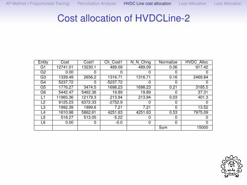
Cost allocation of HVDCLine-2
Entity Cost Cost1 Ch_Cost1 N_N_Chng Normalize HVDC_AllocG1 12741.01 13230.1 489.09 489.09 0.06 917.42G2 0.00 0 0 0 0 0G3 1339.49 2656.2 1316.71 1316.71 0.16 2469.84G4 5237.72 0 -5237.72 0 0 0G5 1776.27 3474.5 1698.23 1698.23 0.21 3185.5G6 5442.47 5462.36 19.89 19.89 0 37.31L1 11965.36 12179.3 213.94 213.94 0.03 401.3L2 9125.23 6372.33 -2752.9 0 0 0L3 1992.39 1999.6 7.21 7.21 0 13.52L4 1610.98 5862.61 4251.63 4251.63 0.53 7975.09L5 518.27 513.05 -5.22 0 0 0L6 0.00 0 -0.0 0 0 0
Sum 15000

AP Method ( Proportionate Tracing) Perturbation Analysis HVDC Line cost allocation Loss Allocation Loss Allocation
Cost allocation of HVDCLines
Entity Psch Cost HVDC_Alloc1 HVDC_Alloc2 Final_Alloc POCG1 3343.37 12741.01 917.42 8219.86 21778.29 6.514G2 3400 0.00 0 0 0 0.0000G3 4800 1339.49 2469.84 2876.11 6684.045 1.3925G4 3400 5237.72 0 74.5 5409.22 1.5624G5 200 1776.27 3185.5 116.62 5093.39 25.3920G6 600 5442.47 37.31 0 5478.78 9.1330L1 4600 11965.36 401.3 0 12359.66 2.6884L2 5300 9125.23 0 7886.8 17015.02 3.2098L3 300 1992.39 13.52 1296.31 3290.23 10.977L4 3500 1610.98 7975.09 735.69 10330.77 2.9491L5 1700 518.27 0 8794.1 9312.97 5.4779L6 300 0.00 0 0 0.0 0.0

AP Method ( Proportionate Tracing) Perturbation Analysis HVDC Line cost allocation Loss Allocation Loss Allocation
Hybrid Method for Sharing of Inter-state TransmissionLosses - CERC Regulations,2010
• The change in the losses because of incrementalinjection/drawal at each node are computed
• The change in overall system losses per unit ofinjection/drawal at each node is termed as Marginal LossFactor
Ki =∂System losses
∂Power injection/drawal at node i

AP Method ( Proportionate Tracing) Perturbation Analysis HVDC Line cost allocation Loss Allocation Loss Allocation
Hybrid Method for Sharing of Inter-state TransmissionLosses - CERC Regulations,2010 (cont.)
• Loss Allocation factors for generation and demand nodesare computed by:
LAF (Pgi ) =
Ki × Pgi∑
i Ki × Pgi +
∑j Kj × Pd
j
LAF (Pdj ) =
Kj × Pdj∑
j Kj × Pdj +
∑i Ki × Pg
i
wherePg
i = base case generation at node i
Pdj = base case drawal at node j
•∑
LAF (Pgi ) +
∑LAF (Pd
j ) = 1
AP Method ( Proportionate Tracing) Perturbation Analysis HVDC Line cost allocation Loss Allocation Loss Allocation
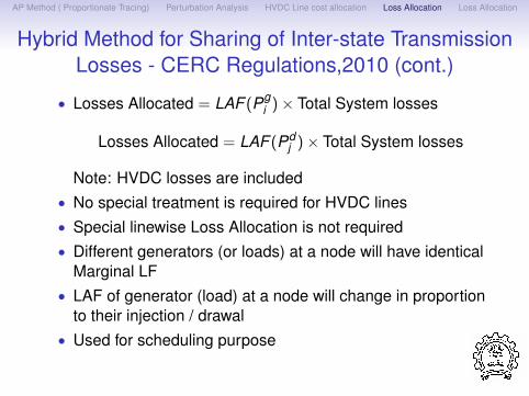
Hybrid Method for Sharing of Inter-state TransmissionLosses - CERC Regulations,2010 (cont.)
• Losses Allocated = LAF (Pgi )× Total System losses
Losses Allocated = LAF (Pdj )× Total System losses
Note: HVDC losses are included• No special treatment is required for HVDC lines• Special linewise Loss Allocation is not required• Different generators (or loads) at a node will have identical
Marginal LF• LAF of generator (load) at a node will change in proportion
to their injection / drawal• Used for scheduling purpose

AP Method ( Proportionate Tracing) Perturbation Analysis HVDC Line cost allocation Loss Allocation Loss Allocation
Marginal Loss and Loss Factor
Entity TL-1 TL-2 TL-3 TL-4 TL-5 TL-6 TL-7 TL-8 TL-9G1 0.0003 0.0095 0.0007 -0.0001 0.0000 0.0080 0.0082 0.0000 0.0000G2 0.0000 0.0001 0.0000 0.0000 0.0000 0.0000 0.0000 0.0000 0.0000G3 0.0009 0.0008 -0.0001 0.0000 0.0000 -0.0004 -0.0003 0.0000 0.0000G4 0.0000 0.0001 0.0000 0.0001 0.0000 0.0000 0.0001 0.0000 0.0000G5 0.0009 0.0009 0.0000 0.0004 0.0035 -0.0004 -0.0002 -0.0001 0.0000G6 0.0032 0.0104 0.0007 0.0000 0.0000 0.0058 0.0053 0.0000 0.0048L1 0.0028 0.0061 0.0002 0.0000 0.0000 0.0021 0.0020 0.0000 0.0005L2 -0.0006 0.0016 0.0003 0.0001 0.0001 0.0020 0.0018 0.0000 0.0001L3 -0.0042 0.0107 -0.0026 0.0000 0.0000 0.0143 0.0254 0.0000 0.0003L4 -0.0004 0.0009 0.0002 -0.0001 -0.0001 0.0011 0.0010 0.0000 0.0000L5 0.0000 0.0000 0.0000 0.0000 0.0000 0.0000 0.0000 0.0000 0.0003L6 0.0000 0.0000 0.0000 0.0000 0.0000 0.0000 0.0000 0.0000 0.0000
lossfactor =∂systemloss∂schedule
(1)

AP Method ( Proportionate Tracing) Perturbation Analysis HVDC Line cost allocation Loss Allocation Loss Allocation
Weighted Marginal loss
Entity Psch LossFactor WLF N-WLF LossAllocG1 3343.28 0.0266 88.831 0.390 17.23G2 3400 0.0001 0.340 0.0001 0.036G3 4800 0.0009 4.320 0.019 0.8641G4 3400 0.0003 0.884 0.0024 0.0972G5 200 0.0050 1.006 0.0045 0.1926G6 600 0.0302 18.108 0.080 3.505L1 4600 0.0137 63.066 0.277 12.08L2 5300 0.0053 28.355 0.1125 5.10L3 300 0.0439 13.170 0.0584 2.5364L4 3500 0.0026 9.030 0.0390 1.6598L5 1700 0.0003 0.510 0.002 0.0956L6 300 0.0000 0.000 0.000 0.0010
WLF is Weighted Loss FactorN-WLF is normalized Weighted Loss FactorTotal loss of the system is: 43.372 MW
AP Method ( Proportionate Tracing) Perturbation Analysis HVDC Line cost allocation Loss Allocation Loss Allocation
Discussion!..........

AP Method ( Proportionate Tracing) Perturbation Analysis HVDC Line cost allocation Loss Allocation Loss Allocation
Thank you..