Transmission Expansion Planning with Re-design

Luciano S. Moulin ∗ Michael Poss † Claudia Sagastizabal ‡

May 17, 2010

Abstract

Expanding an electrical transmission network requires heavy investments that need to becarefully planned, often at a regional or national level. We study relevant theoretical andpractical aspects of transmission expansion planning, set as a bilinear programming problemwith mixed 0-1 variables. We show that the problem is NP-hard and that, unlike the so-calledNetwork Design Problem, a transmission network may become more efficient after cutting-offsome of its circuits. For this reason, we introduce a new model that, rather than just addingcapacity to the existing network, also allows for the network to be re-designed when it isexpanded. We then turn into different reformulations of the problem, that replace the bilinearconstraints by using a “big-M” approach. We show that computing the minimal values forthe “big-M” coefficients involves finding the shortest and longest paths between two buses.We assess our theoretical results by making a thorough computational study on real electricalnetworks. The comparison of various models and reformulations shows that our new model,allowing for re-design, can lead to sensible cost reductions.

Keywords: transmission network, network design, “big-M” formulation.

1 Introduction

Long term transmission expansion planning determines, over an horizon of 10 or more years,optimal investments on new transmission lines that make up an economic and reliable electricalnetwork. In its general form, transmission expansion planning is set as a mixed-integer nonlinearstochastic programming problem that minimizes discounted expected costs of investment, subjectto constraints depending on uncertain data, such as future growth of electricity demand and ofgeneration.

Historically, transmission expansion planning stems from centralized systems, with both gener-ation and transmission assets belonging to the government. In this setting, transmission planningshould ideally be performed jointly with the generation expansion. However, since the resultingoptimization problem would be too complex to handle, electrical transmission and energy genera-tion expansion plans are often determined separately, at least for large power systems. Once bothexpansion plans are available, they can be used as input for some integrated model of generationand transmission, with simplified features. Alternatively, the output of a simplified integratedmodel can be used as input of the separate expansion planning problems.

The interest of transmission expansion planning also extends to competitive frameworks. Thecurrent deregulation trend often results in a mix of market competition in the generation anddistribution sectors, with a centralized regulation for transmission. In this context, the regulatingentity is in charge, not only of operating the grid while maximizing energy trade opportunities,but also of defining an expansion plan for the transmission network to remain operational in thefuture. Whether the power system is centralized or liberalized, transmission expansion planningis a valuable tool for helping the decision-maker in adopting the most appropriate strategies fordetermining the time, the location, and the type of transmission lines to be built.

∗CEPEL, Electric Energy Research Center, Eletrobras Group. moulin@cepel.br†Department of Computer Science, Universite Libre de Bruxelles, Brussels, Belgium. mposs@ulb.ac.be‡CEPEL, Electric Energy Research Center, Eletrobras Group. On leave from INRIA Rocquencourt, France.

sagastiz@impa.br

1

The transmission expansion planning problem is set over an electrical network, designed in thepast by taking into account some critical factors, specific to the power system under consideration.The amount of hydropower is crucial in hydro-dominated power systems like Brazil’s, becausegeneration sites are usually far away from the consumption centers. Long transmission lines and,hence, important investments, are needed. Also, due to the pluvial regime, the network needs toaccommodate various power flows arising in different hydrological conditions. Another importantfactor is the demand growth rate along the years, especially for countries with significant growthrates, which need large investments and a large portfolio with reinforcement candidates.

The transmission expansion planning optimization problem includes both physical and budgetconstraints. Operational and investment constraints are often linear, and vary dynamically alongthe planning horizon. By contrast, expansion transmission constraints are static and nonconvex,generally bilinear. Due to the high complexity and difficulty of the corresponding optimizationproblem, several simplified models and approximation techniques have been considered; see thereview [22]. For example, in [30], the transmission expansion planning problem with security con-straints, preventing transmission equipment failure, is set as two-stage stochastic mixed-integerlinear program, decomposed by Benders technique and solved by a (multicut) cutting-planes al-gorithm, [8]. If transmission losses are a concern, they can be treated by a linearization, as in[15, 16].

Due to the restructuration of the electrical sector that affected many countries in the recentyears, uncertainty has lately arisen as an important consideration. This impacts the modelling andsignificantly increases the size and complexity of the optimization problem. Reported results aremostly for small power systems (6 to 30 buses) [35, 12, 25]; see also [10, 11, 17, 43, 9, 23, 24, 34, 15].When considering larger power systems, the problem size is reduced by some heuristic method,relying on human experts’ judgment, as in [37, 29, 28, 10].

In general, the transmission expansion planning problem is solved in two variants, consideringor not generation redispatch; see [4, 14, 16]. The case without redispatch requires the plannedtransmission network to operate correctly for a given set of generation values, computed apriorifor each generation plant. The variant with redispatch considers generation as a variable in theoptimization problem: an economic dispatch and the optimal transmission expansion plan arecomputed together.

In this work, we propose a transmission expansion planning model that, rather than just addingcapacity to the existing network, also allows for the network to be re-designed when it is expanded.Our new modelling introduces more flexibility and is general, in the sense that it can be used fordifferent frameworks, with and without redispatch, and independently of the level of simplificationor sophistication of the formulation, including with respect to uncertainty treatement.

The new model with re-design relies on the observation that an existing transmission network,designed in the past, may no longer be optimal in the present and it may become even lesswell adapted in the future. In the transmission expansion planning problem, electrical powerflows in the grid according to the linearized second Kirchoff’s law, and has the following peculiarproperty, unique to electrical networks. Namely, in some configurations, disconnecting an existenttransmission line (respectively, adding a new line) does not necessarily decrease (respectively,increase) the network capacity. Our numerical testing shows that allowing for the network to bere-designed while expanding it can result in significant savings.

Our paper is organized as follows. In Section 2, we start with a general transmission expansionplanning problem, then present our model with re-design, and comment on alternative modelsproposed by some authors. As mentioned, the transmission expansion planning problem has bi-linear constraints that need to be dealt with. Section 3 contains a mathematical study comparingdifferent disjunctive proposals that can be found in the literature. Some alternative linearizationtechniques, improving the relaxed transmission expansion planning problem, are also analyzed. Inmost of the proposals, bilinear constraints are “linearized” by using the “big-M” reformulationfrom Disjunctive Programming. The problem of choosing suitable values for the corresponding“big-M” coefficients is addressed in Section 4. We first give general minimum values for the modelswith and without re-design, and then analyze how to exploit the initial network topology to reducethe minimal bounds. Section 5 reports on our numerical testing, including a thorough comparisonof the various formulations performances on several grids of real size. The final Section 6 gives themodel with re-design when considering (N − 1) security constraints, some preliminary numericalexperience, and a discussion on how to handle uncertain demand and generation.

2

List of Symbols

S bus-circuit incidence matrix

i ∈ B index bus, in the set of buses

gi maximal generation at bus i

di load at bus i

Ω = Ω0 ∪ Ω1 set of all circuits

Ω0 set of existing circuits

Ω1 set of candidate circuits

|Ω1| cardinality of set Ω1

i(k), j(k) terminal buses of circuit k

γk susceptance of circuit k

fk capacity of circuit k

ck investment cost of circuit k

k1 ∦ k2 not parallel circuits

k1 ‖ k2 parallel circuits

E = E0 ∪ E1 set of all “fat” edges

E0 set of “fat” edges containing existing circuits

E1 set of “fat” edges containing candidate circuits

xij maximum number of circuits that can be built between i and j

xij existing number of circuits between i and j

(ij) “fat” edge between i and j

` ∈ Lij index circuit among all circuits belonging to “fat” edge (ij)

SPi−j shortest path between buses i and j

LPi−j longest path between buses i and j

LP li−j longest path between buses i and j not passing through bus l

2 Models for transmission expansion planning

For convenience, we start by formulating a deterministic transmission expansion planning problemwithout contingencies; in Section 6, we consider how to incorporate uncertainty and (N − 1)constraints in the modelling. From the Combinatorial Optimization point of view, the electricalnetwork is an undirected graph (B,Ω) where vertices i ∈ B are called buses and edges k ∈ Ω arecalled circuits. The set of circuits is partitioned into a subset Ω0, of existing circuits, and a disjointsubset of candidate circuits, denoted by Ω1. Circuits are connected to buses in a linear relationgiven by S, the bus-circuit incidence matrix. For each circuit k ∈ Ω, indices i(k) and j(k) denote,respectively, the head and the tail of the circuit, while γk is the circuit susceptance. The referencebus angle is fixed at θref = 0. The grid can have parallel circuits, k1, k2 ∈ Ω, denoted by k1 ‖ k2,linking the same terminal buses.

3

2.1 Classical transmission expansion planning problem

The transmission network expansion problem is usually written in the following form:

(TEP)

min∑k∈Ω1

ckxk

s.t. Sf + g = d (Load)fk − γk(θi(k) − θj(k)) = 0 k ∈ Ω0 (Kirchoff0)fk − γkxk(θi(k) − θj(k)) = 0 k ∈ Ω1 (Kirchoff1)

|fk| ≤ fk k ∈ Ω (FlowBounds)0 ≤ gi ≤ gi i ∈ B (GenBounds)xk ∈ 0, 1 k ∈ Ω1 .

At first glance, problem (TEP) could be considered as a Capacitated Network Design problem,used to model expansion of telecommunication networks [42] and freight transportation networks[13], among others. However, there is one important difference, that has a crucial impact whensolving the transmission expansion planning problem. Specifically, most capacitated problemssatisfy the following property:

for any given x ∈ 0, 1|Ω1|, with components xk =

1 for k ∈ Ω′ ⊂ Ω1

0 for k ∈ Ω1\Ω′,if x is feasible for (TEP), then any vector x ∈ 0, 1|Ω1| such that x ≥ x is also feasible for (TEP).

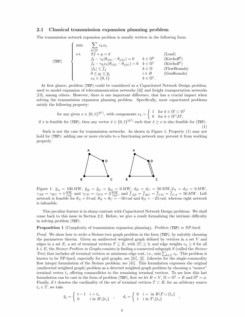
(1)Such is not the case for transmission networks. As shown in Figure 1, Property (1) may not

hold for (TEP): adding one or more circuits to a functioning network may prevent it from workingproperly.

Figure 1: gA = 100MW , gB = gC = gD = 0MW , dB = dC = 50MW,dA = dD = 0MW ,γAB = γBC = 1MW

rad and γCD = γDA = 2MWrad , and fAB = fBC = fCD = fCA = 50MW . Left

network is feasible for θA = 0 rad, θB = θC = −50 rad and θD = −25 rad, whereas right networkis infeasible.

This peculiar feature is in sharp contrast with Capacitated Network Design problems. We shallcome back to this issue in Section 2.2. Before, we give a result formalizing the intrinsic difficultyin solving problem (TEP).

Proposition 1 (Complexity of transmission expansion planning). Problem (TEP) is NP-hard.

Proof. We show how to write a Steiner-tree graph problem in the form (TEP), by suitably choosingthe parameters therein. Given an undirected weighted graph defined by vertices in a set V andedges in a set E, a set of terminal vertices T ⊆ E, with |T | ≥ 3, and edge weights ck ≥ 0 for allk ∈ E, the Steiner Problem in Graphs consists in finding a connected subgraph S (called the SteinerTree) that includes all terminal vertices at minimum edge cost, i.e., min

∑k∈S ck. This problem is

known to be NP-hard, especially for grid graphs, see [21], [2]. Likewise for the single-commodityflow integer formulation of the Steiner problem; see [41]. This formulation expresses the original(undirected weighted graph) problem as a directed weighted graph problem by choosing a “source”terminal vertex ts offering commodities to the remaining terminal vertices. To see how this lastformulation can be cast in the form of problem (TEP), first we let B = V , Ω = Ω1 = E and Ω0 = φ.Finally, if t denotes the cardinality of the set of terminal vertices T ⊂ B, for an arbitrary sourcets ∈ T , we take

gi =

t− 1 i = ts0 i in B\ts

, di =

0 i = in B\T ∪ ts1 i in T\ts

,

4

and, for all k ∈ Ω, fk ≥ t− 1 and γk = 1. With this data, an optimal solution to (TEP) is nothingbut a minimum cost Steiner tree connecting vertices in T .

2.2 Allowing for the network to be re-designed

In network design problems, new links are added to a network to make it capable of routinggiven commodities. Typical examples of commodities are passengers using public transportation,merchandise in a vehicle routing problem, data in a telecommunication network, or electricity in atransmission grid.

As mentioned, the peculiar behavior of power flow makes transmission networks very differentfrom the other examples. In particular, for most network design problems, the routing is eitherdecided by some manager, or fixed by a rule aiming at minimizing some utility (congestion, traveltime, travel costs). In such circumstances, the fact of adding a new link to a functioning networkcan never prevent the network from working properly. At worst, the manager can decide not to usethat particular link. By constrast, in transmission power systems, the network manager cannotchoose which circuits will be used. Only generation dispatch, indirectly affecting the routing,can be chosen (generation levels are control variables, while voltage angles and flows are statevariables). The example in Figure 1 shows that, besides being useless, a new link can also makethe network inoperational. Similarly, an inoperational network unable to satisfy its load could insome cases start functioning after cutting-off some of its circuits.

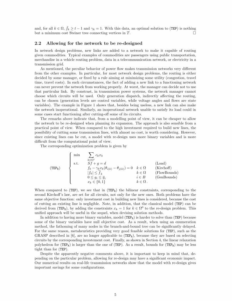
The remarks above indicate that, from a modelling point of view, it can be cheaper to allowthe network to be re-designed when planning its expansion. The approach is also sensible from apractical point of view. When compared to the high investment required to build new lines, thepossibility of cutting some transmission lines, with almost no cost, is worth considering. However,since existing lines can be cut, a model with re-design uses more binary variables and is moredifficult from the computational point of view.

The corresponding optimization problem is given by

(TEPR)

min∑k∈Ω1

ckxk

s.t. Sf + g = d (Load)fk − γkxk(θi(k) − θj(k)) = 0 k ∈ Ω (Kirchoff)

|fk| ≤ fk k ∈ Ω (FlowBounds)0 ≤ gi ≤ gi i ∈ B (GenBounds)xk ∈ 0, 1 k ∈ Ω .

When compared to (TEP), we see that in (TEPR) the bilinear constraints, corresponding to thesecond Kirchoff’s law, are set for all circuits, not only for the new ones. Both problems have thesame objective function: only investment cost in building new lines is considered, because the costof cutting an existing line is negligible. Note, in addition, that the classical model (TEP) can bederived from (TEPR), by adding the constraints xk = 1 for k ∈ Ω0 to the re-design problem. Thisunified approach will be useful in the sequel, when devising solution methods.

In addition to having more binary variables, model (TEPR) is harder to solve than (TEP) becausesome of the binary variables have null objective cost. As a result, when using an enumerationmethod, the fathoming of many nodes in the branch-and-bound tree can be significantly delayed.For the same reason, metaheuristics providing very good feasible solutions for (TEP), such as theGRASP described in [6], are no longer applicable to (TEPR), because they are based on selectingcircuits by the corresponding investement cost. Finally, as shown in Section 4, the linear relaxationpolyhedron for (TEPR) is larger than the one of (TEP). As a result, bounds for (TEPR) may be lesstight than for (TEP).

Despite the apparently negative comments above, it is important to keep in mind that, de-pending on the particular problem, allowing for re-design may have a significant economic impact.Our numerical results on real-life transmission networks show that the model with re-design givesimportant savings for some configurations.

5

2.3 Simplified related models

Both (TEP) and (TEPR) can be further complicated by the introduction of (N − 1) security con-straints. These constraints state that if, for some contingency, any circuit happens to fail (alone),the network must stay functional. We will come back to this issue in Section 6.

In view of the difficulty of the transmission expansion planning problem, even without contin-gencies, several authors introduced simplified models that we review next. However, in all of themodels below, simplification comes at the stake of ending up with a network for which (1) holds.Since this property is not satisfied by a transmission network, for some applications the (simplified)optimal plan computed with such models may need to be modified when the network is actuallyexpanded.

In [5] the model is set to find a minimal cost capacity increase that ensures the network survivalto different failures. The network is represented by a graph without parallel edges, and each edge khas an initial capacity, denoted by uk. Parallel circuits are summed up into a single edge with thecorresponding total capacity. In the absence of parallel edges, bilinear constraints can be avoidedby replacing, for all k ∈ Ω, constraints (Kirchoff) and (FlowBounds) by

fk − γk(θi(k) − θj(k)) = 0 and |fk| ≤ uk + fkxk ,

respectively. Failures are considered in two different variants, depending if they occur simultane-ously or in cascade. The first variant is solved by an efficient Benders decomposition scheme. Thesolution method for the second variant makes use of strong valid inequalities in a cutting planesframework. For both variants, the elimination of parallel circuits allows the authors to solve muchbigger instances than the ones handled in our numerical results.

Another simplified model goes back to Garver’s transportation model [18], where (Kirchoff1)is replaced by a flow constraint of the form |fk| ≤ xkfk for all k ∈ Ω1. The resulting mixed-integer linear programming problem is easy to solve by modern solvers, because it is closely relatedto the so-called single-commodity multi-facility capacitated network design problem. Althoughunrealistic, the transportation model can provide a better lower bound for (TEP) and (TEPR) thanthe optimal value of the linear relaxation, see Table 5 in Section 5. Hence, it can be efficientlyused in a branch-and-bound process to eliminate portions of the exploration tree.

The third model in our review was proposed in [36] for electricity distribution. Due to thelocal span of distribution networks, there is one generating unit (only one generation bus) and thenetwork must be a tree (each pair of buses is connected by a single path). In this setting, themodel is no longer a simplification, because the actual network satisfies (1).

The tree requirement introduces many combinatorial affine constraints. In counterpart, weshow below that a tree network makes the (bilinear) second Kirchoff’s law redundant, simplifyingsubstantially the optimization problem (voltage angles disappear from the formulation).

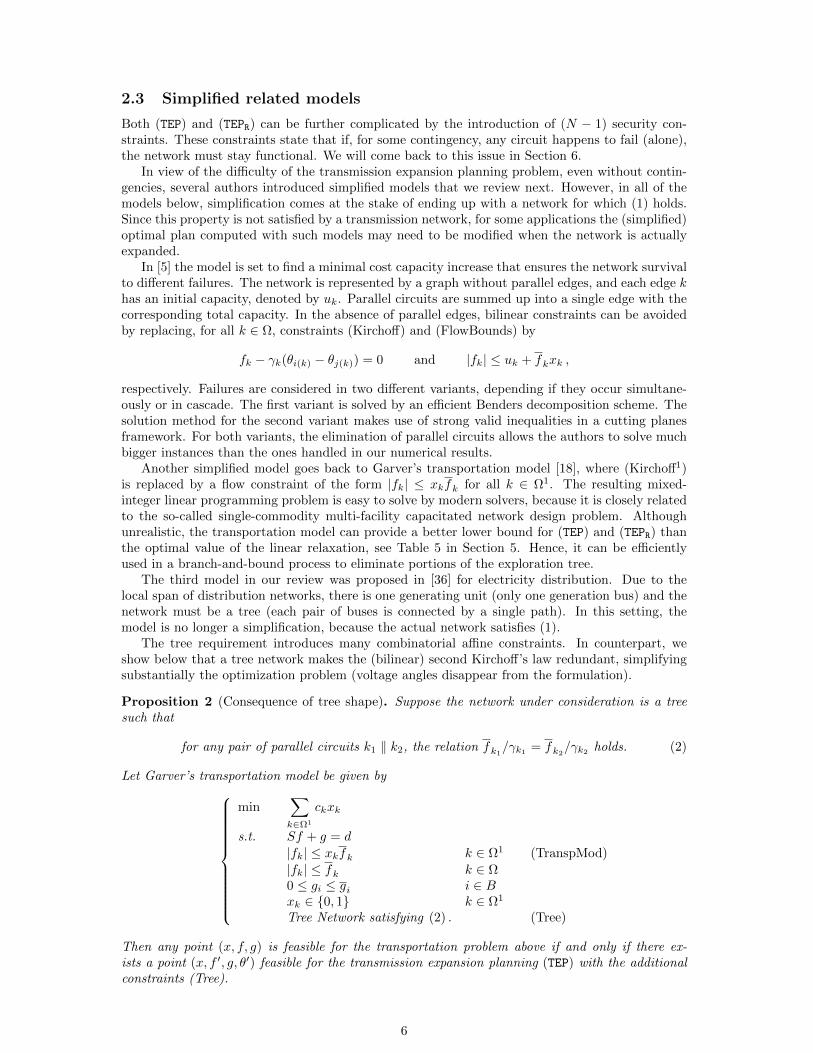
Proposition 2 (Consequence of tree shape). Suppose the network under consideration is a treesuch that

for any pair of parallel circuits k1 ‖ k2, the relation fk1/γk1 = fk2/γk2 holds. (2)

Let Garver’s transportation model be given by

min∑k∈Ω1

ckxk

s.t. Sf + g = d

|fk| ≤ xkfk k ∈ Ω1 (TranspMod)

|fk| ≤ fk k ∈ Ω0 ≤ gi ≤ gi i ∈ Bxk ∈ 0, 1 k ∈ Ω1

Tree Network satisfying (2) . (Tree)

Then any point (x, f, g) is feasible for the transportation problem above if and only if there ex-ists a point (x, f ′, g, θ′) feasible for the transmission expansion planning (TEP) with the additionalconstraints (Tree).

6

Proof. The necessary condition is straightforward, because the feasible set of the transmissionexpansion planning (TEP) is contained in the feasible set of the transportation model. To prove thereverse inclusion, given (x, f, g) feasible for the transportation model, we define a point (x′, f ′, g′, θ′)that is feasible for (TEP), as follows. First, we keep the same design variables, x′k = xk for eachk ∈ Ω, and generation variables, g′i = gi for each i ∈ B. Then, we consider any circuit k ∈ Ω withendpoints i and j. The total flow between i and j is bounded by the total capacity of the circuitsconnecting i and j, so that their ratio Fij is smaller than one:

Fij ≡∑h∈Ω:h‖k fh∑

h∈Ω1:h‖k xhfh +∑h∈Ω0:h‖k fh

≤ 1.

Then, f ′k = fkFij ≤ fk for k ∈ Ω0 and f ′k = xkfkFij ≤ fk for k ∈ Ω1 so that f ′ satisfies the(FlowBounds) constraints. The constraint (Load) for any b1 ∈ B is also satisfied, because gb1 isequal to g′b1 and the total flow from b1 to any b2 ∈ B is unchanged: for any k ∈ Ω such thati(k) = b1 and j(k) = b2, the total flow between b1 and b2 is given by

∑h∈Ω:h||k

f ′h = Fb1b2

∑h∈Ω1:h‖k

xhfh +∑

h∈Ω0:h‖k

fh

=∑

h∈Ω:h‖k

fh.

The new flow vector f ′ allows us to set up feasible voltage angles θ′ satisfying (Kirchoff0) and(Kirchoff1), as follows. First, we choose any bus ref ∈ B and set θ′ref = 0. Then, we select any

built circuit k (k ∈ Ω1 and xk = 1, or k ∈ Ω0) with i(k) = ref and set θ′j(k) = θ′i(k) − f′k/γk =

0 − f ′k/γk = −Fi(k)j(k) fk/γk. Assumption (2) ensures that choosing h ‖ k, instead of k, inducesthe same angles difference. Next, we select a built circuit h ∦ k with i(h) ∈ ref, j(k) to set upθ′j(h) in the same way. We repeat this procedure until all voltage angles are set, the tree shapeensuring that each of them shall be set only once.

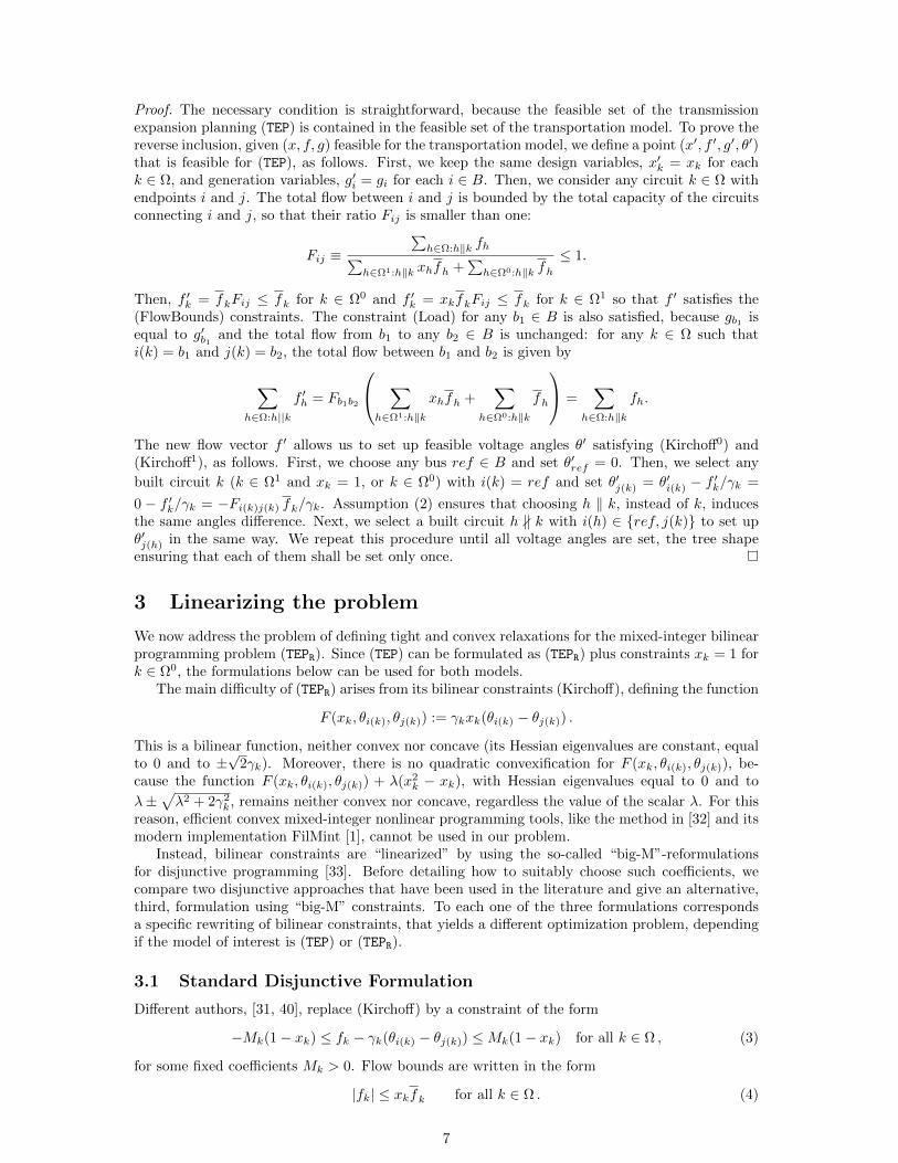
3 Linearizing the problem

We now address the problem of defining tight and convex relaxations for the mixed-integer bilinearprogramming problem (TEPR). Since (TEP) can be formulated as (TEPR) plus constraints xk = 1 fork ∈ Ω0, the formulations below can be used for both models.

The main difficulty of (TEPR) arises from its bilinear constraints (Kirchoff), defining the function

F (xk, θi(k), θj(k)) := γkxk(θi(k) − θj(k)) .

This is a bilinear function, neither convex nor concave (its Hessian eigenvalues are constant, equalto 0 and to ±

√2γk). Moreover, there is no quadratic convexification for F (xk, θi(k), θj(k)), be-

cause the function F (xk, θi(k), θj(k)) + λ(x2k − xk), with Hessian eigenvalues equal to 0 and to

λ±√λ2 + 2γ2

k, remains neither convex nor concave, regardless the value of the scalar λ. For thisreason, efficient convex mixed-integer nonlinear programming tools, like the method in [32] and itsmodern implementation FilMint [1], cannot be used in our problem.

Instead, bilinear constraints are “linearized” by using the so-called “big-M”-reformulationsfor disjunctive programming [33]. Before detailing how to suitably choose such coefficients, wecompare two disjunctive approaches that have been used in the literature and give an alternative,third, formulation using “big-M” constraints. To each one of the three formulations correspondsa specific rewriting of bilinear constraints, that yields a different optimization problem, dependingif the model of interest is (TEP) or (TEPR).

3.1 Standard Disjunctive Formulation

Different authors, [31, 40], replace (Kirchoff) by a constraint of the form

−Mk(1− xk) ≤ fk − γk(θi(k) − θj(k)) ≤Mk(1− xk) for all k ∈ Ω , (3)

for some fixed coefficients Mk > 0. Flow bounds are written in the form

|fk| ≤ xkfk for all k ∈ Ω . (4)

7

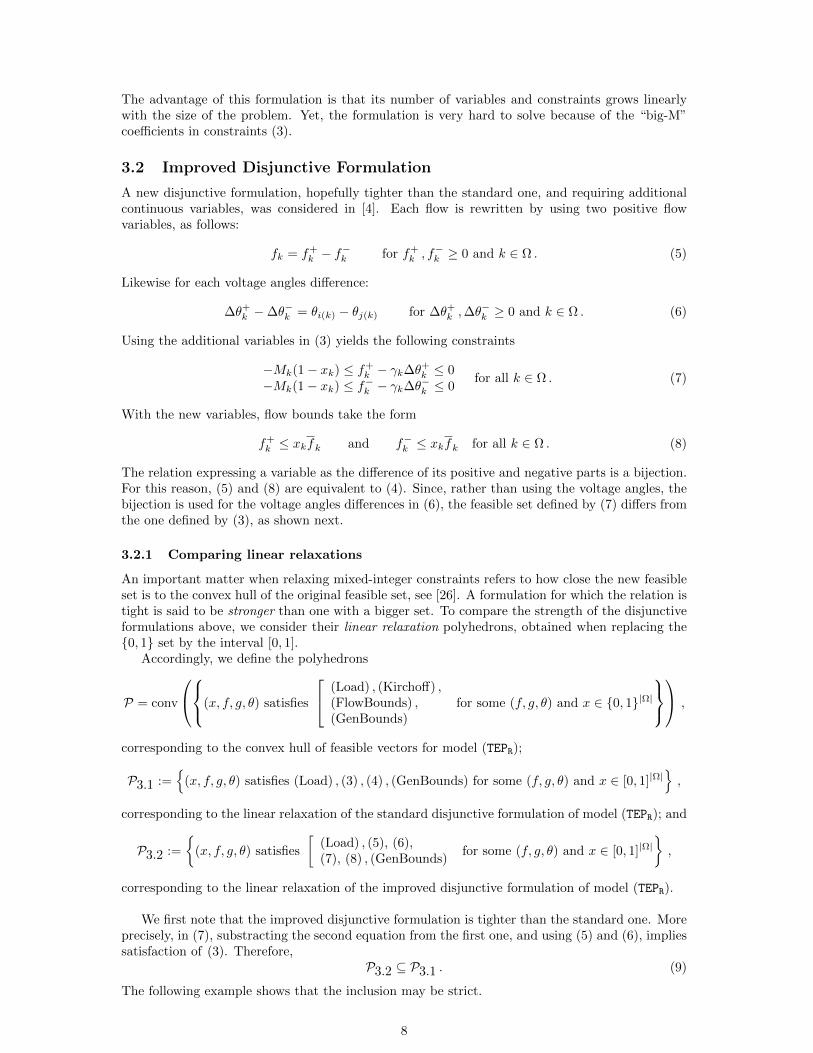
The advantage of this formulation is that its number of variables and constraints grows linearlywith the size of the problem. Yet, the formulation is very hard to solve because of the “big-M”coefficients in constraints (3).

3.2 Improved Disjunctive Formulation

A new disjunctive formulation, hopefully tighter than the standard one, and requiring additionalcontinuous variables, was considered in [4]. Each flow is rewritten by using two positive flowvariables, as follows:

fk = f+k − f

−k for f+

k , f−k ≥ 0 and k ∈ Ω . (5)

Likewise for each voltage angles difference:

∆θ+k −∆θ−k = θi(k) − θj(k) for ∆θ+

k ,∆θ−k ≥ 0 and k ∈ Ω . (6)

Using the additional variables in (3) yields the following constraints

−Mk(1− xk) ≤ f+k − γk∆θ+

k ≤ 0−Mk(1− xk) ≤ f−k − γk∆θ−k ≤ 0

for all k ∈ Ω . (7)

With the new variables, flow bounds take the form

f+k ≤ xkfk and f−k ≤ xkfk for all k ∈ Ω . (8)

The relation expressing a variable as the difference of its positive and negative parts is a bijection.For this reason, (5) and (8) are equivalent to (4). Since, rather than using the voltage angles, thebijection is used for the voltage angles differences in (6), the feasible set defined by (7) differs fromthe one defined by (3), as shown next.

3.2.1 Comparing linear relaxations

An important matter when relaxing mixed-integer constraints refers to how close the new feasibleset is to the convex hull of the original feasible set, see [26]. A formulation for which the relation istight is said to be stronger than one with a bigger set. To compare the strength of the disjunctiveformulations above, we consider their linear relaxation polyhedrons, obtained when replacing the0, 1 set by the interval [0, 1].

Accordingly, we define the polyhedrons

P = conv

(x, f, g, θ) satisfies

(Load) , (Kirchoff) ,(FlowBounds) ,(GenBounds)

for some (f, g, θ) and x ∈ 0, 1|Ω| ,

corresponding to the convex hull of feasible vectors for model (TEPR);

P3.1 :=

(x, f, g, θ) satisfies (Load) , (3) , (4) , (GenBounds) for some (f, g, θ) and x ∈ [0, 1]|Ω|,

corresponding to the linear relaxation of the standard disjunctive formulation of model (TEPR); and

P3.2 :=

(x, f, g, θ) satisfies

[(Load) , (5), (6),(7), (8) , (GenBounds)

for some (f, g, θ) and x ∈ [0, 1]|Ω|,

corresponding to the linear relaxation of the improved disjunctive formulation of model (TEPR).

We first note that the improved disjunctive formulation is tighter than the standard one. Moreprecisely, in (7), substracting the second equation from the first one, and using (5) and (6), impliessatisfaction of (3). Therefore,

P3.2 ⊆ P3.1 . (9)

The following example shows that the inclusion may be strict.

8

Example 1 (Strict inclusion). Consider a network formed by three buses A ,B, and C, with noinitial circuits and such that at most one circuit connecting each pair of buses can be built. Suppose,in addition, that the parameters have the values gA = 100MW , gB = gC = 0, dA = dC = 0,dB = 100MW , fAB = fBC = fCA = 400MW , γAB = γCA = 1MW

rad and γBC = 0.5MWrad and

cAB = cBC = cCA = 10. The optimal value to the transmission expansion planning optimizationproblem (TEPR) is 10, obtained by constructing only circuit AB: xAB = 1, the remaining optimalbinary variables being null. The corresponding voltage angles at the optimum are θA = 0 rad andθB = −100 rad. We show next how to construct a cheaper fractional solution (x, f, g, θ) in P3.1that does not belong to P3.2.

In Section 4 we give the smallest values for the “big-M” coefficients to ensure a tight relaxation.In particular, by Proposition 3 therein, the minimal value for MBC is 400MW . Consider thefractional vector xAB = xBC = xCA = 0.25, with angles θA = 0, θB = θC = −50 rad and flowsfAC = fCB = fAB = 50MW . The corresponding objective function value is 7.5, smaller than theoptimal cost of the mixed 0-1 problem.

For the point under consideration, the potential differences γAB(θA − θB) = γAC(θA − θC) =50MW are enough to induce the required flows, whereas γCB(θC−θB) = 0MW should not induceany flow. However, since x is fractional, the “big-M” constraints may allow this flow to be routedon the network. Namely, constraint (3) for circuit CB is

−300 ≤ fCB ≤ 300 ,

while constraint (7) for circuit CB isfCB = 0. (10)

Thus, the flows fAC = fCB = fAB = 50MW give a feasible point in P3.1. By contrast, constraints(10) will cut-off the point from P3.2.

For a linear relaxation to be useful for the optimization problem, its “shadow” projection onthe x-variables (see [26]) needs to be tight with respect to the original problem. This means thatin the relaxed polyhedrons only the x-components of feasible vectors (x, f, g, θ) matter.

In this sense, although the inclusion (9) ensures a similar relation for the shadow projections,we are in no position to say if the inclusion is strict for the x-variables only. In particular, we nowshow that for the counter-example above, it is possible to define flows and angles f , θ satisfying(7) for the fractional values xAB = xBC = xCA = 0.25.

Example 2 (No longer strict inclusion). Consider the network in Example 1 and the same frac-tional vector xAB = xBC = xCA = 0.25. Set angles to θA = θC = 0 rad and θB = −100 rad, andflows to fAB = 100MW , fAC = fCB = 0MW . Such flows fAB and fAC are correctly inducedby the potential differences, as long as the flow fCB is equal to 50MW . However, recalling thatMBC(1− xBC) = 300MW , constraint (7) for circuit CB is

−250 ≤ fCB ≤ 50, (11)

so that fCB = 0MW is feasible for (11) and (x, f , θ, g) ∈ P3.2.

In summary, from relation (9), the linear relaxation of the improved disjunctive formulationis not worse than the one of the standard disjunctive formulation. But it is not known if, whenconsidering only the x-components, the inclusion remains strict (unfortunately, no example is givenin [4]). In our computational experience in Section 5, both disjunctive formulations gave identicalresults, for all the cases in Table 1.

3.3 Breaking Symmetry

In Combinatorial Optimization, it is well known that feasible sets exhibiting symmetry oftenslow down significantly any branch-and-bound algorithm, due to (useless) exploration of manysymmetric nodes. In a transmission network, parallel circuits do induce such a symmetry, makingboth disjunctive formulations in Sections 3.1 and 3.2 difficult to solve.

9

Basically, parallel circuits yield feasible points that are indistinguishable by the objective func-tion. Indeed, from a feasible vector involving parallel circuits k1 ‖ k2, another feasible vector withthe same cost can be obtained, simply by swapping indices corresponding to k1 and k2.

In order to address this important issue, in what follows we assume the condition below.

Assumption 1. Any pair of parallel circuits k1, k2 ∈ Ω has the same capacity, susceptance andcost:

∀k1 ‖ k2 fk1 = fk2 , γk1 = γk2 , and ck1 = ck2 .

All the case studies considered in our numerical experience, and given in Table 1 below, satisfyAssumption 1.

The interest of Assumption 1 is that it allows us to define new circuit sets, by gathering parallelcircuits into a single, “fat”, edge. We denote such new sets by E0 and E1, corresponding to Ω0

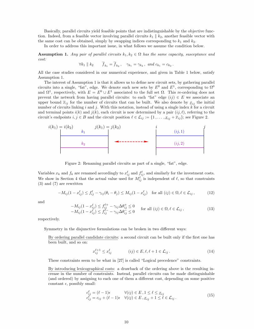
and Ω1, respectively, with E = E0 ∪ E1 associated to the full set Ω. This re-ordering does notprevent the network from having parallel circuits: to each “fat” edge (ij) ∈ E we associate anupper bound xij for the number of circuits that can be built. We also denote by xij the initialnumber of circuits linking i and j. With this notation, instead of using a single index k for a circuitand terminal points i(k) and j(k), each circuit is now determined by a pair (ij, `), referring to thecircuit’s endpoints i, j ∈ B and the circuit position ` ∈ Lij := 1 , . . . , xij + xij; see Figure 2.

k1

k2

i j(ij, 1)

(ij, 2)

j(k1) = j(k2)i(k1) = i(k2)

Figure 2: Renaming parallel circuits as part of a single, “fat”, edge.

Variables xk and fk are renamed accordingly to x`ij and f `ij , and similarly for the investment costs.

We show in Section 4 that the actual value used for M `ij is independent of `, so that constraints

(3) and (7) are rewritten

−Mij(1− x`ij) ≤ f `ij − γij(θi − θj) ≤Mij(1− x`ij) for all (ij) ∈ Ω, ` ∈ Lij , (12)

and−Mij(1− x`ij) ≤ f

`+ij − γij∆θ

+ij ≤ 0

−Mij(1− x`ij) ≤ f`−ij − γij∆θ

−ij ≤ 0

for all (ij) ∈ Ω, ` ∈ Lij , (13)

respectively.

Symmetry in the disjunctive formulations can be broken in two different ways:

By ordering parallel candidate circuits: a second circuit can be built only if the first one hasbeen built, and so on:

x`+1ij ≤ x`ij (ij) ∈ E, `, `+ 1 ∈ Lij . (14)

These constraints seem to be what in [27] is called “Logical precedence” constraints.

By introducing lexicographical costs: a drawback of the ordering above is the resulting in-crease in the number of constraints. Instead, parallel circuits can be made distinguishable(and ordered) by assigning to each one of them a different cost, depending on some positiveconstant ε, possibly small:

c`ij = (`− 1)ε ∀(ij) ∈ E , 1 ≤ ` ≤ xijc`ij = cij + (`− 1)ε ∀(ij) ∈ E , xij + 1 ≤ ` ∈ Lij .

(15)

10

In our numerical tests, the improved disjunctive formulation in Section 3.2 did not give competitiveresults. For this reason, we applied (14) and (15) only to the standard disjunctive formulationfrom Section 3.1. The lexicographical ordering (15) turned out to be rather poor, at least in ourcase studies. For instance, the transmission expansion planning for the network “Brazil South”,modelled by (TEP) and using the standard disjunctive formulation, took 5 seconds to be solveduntil optimality. When introducing (15), solution times climbed up to more than 300 seconds.

We mention that CPLEX 11 has an automatic symmetry breaking procedure which can sensiblyaffect solution times. When this procedure is deactivated, by setting IloCplex.IntParam.Symmetry= 0, the standard disjunctive formulation is much slower than when using the approaches (14) or(15). However, when setting IloCplex.IntParam.Symmetry = -1, the impact of (14) becomes muchless expressive.

3.4 Alternative Disjunctive Formulation

We also considered a third disjunctive formulation, grouping together parallel circuits:

min∑

(ij)∈E1

cij∑

Lij3`≥xij+1

(`− xij)x`ij

s.t. Nf + g = d

−M `ij(1− x`ij) ≤

fij` − γij(θi − θj) ≤M

`ij(1− x`ij) (ij) ∈ E, ` ∈ Lij (BigM)∑

`∈Lijx`ij ≤ 1 (ij) ∈ E (SOS1)

|fij | ≤ f ij∑`∈Lij

` x`ij (ij) ∈ E (FlowCap)

0 ≤ gi ≤ gi i ∈ Bx`ij ∈ 0, 1 ij ∈ E, ` ∈ Lij ,

where N is defined from S by selecting only one column for each “fat” edge (ij) ∈ E. Althoughthis formulation significantly reduces the number of flow variables, such potential advantage wasnot reflected in our computational results; see Section 5. In an effort to improve performance,we also tried CPLEX functionality of using type SOS 1 constraints instead of (SOS1) above. Butthis option was not effective, probably due to the important increase in the number of nodes tobe explored. Setting different values to IloCplex.IntParam.Symmetry did not bring much benefiteither.

4 Choosing suitable “big-M” coefficients

The efficient solution of the linearized disjunctive formulations depends strongly on how the coef-ficients “big-M” are set. Bigger coefficients give less tight polyhedrons, and worse optimal values.It is then worthwhile to compute minimal values, M ij , such that constraints (12), (13) and (BigM)above are valid for P, for any given value of g and d. Recall that an inequality is said to be validfor a polyhedron Q if Q is contained in the half space delimited by the inequality.

We first give general minimum values for the models with and without re-design, and thenanalyze how to exploit the initial network topology (E0) to reduce the minimal bounds.

In our analysis, paths are always assumed without cycles (they cannot contain twice the samenode).

We start with model (TEPR), allowing re-design, noting that, for any vector x ∈ 0, 1|E|, wheng = d = 0, the point (x, f = 0, θ = 0, g = 0) trivially belongs to P. For this reason, the boundfor the “big-M” coefficients should be found for any binary vector x. We now show that thecomputation of such bound involves solving a longest path problem (see [19]).

Proposition 3. Suppose Assumption 1 holds and let (ij) be given. Consider constraints (12) and(13) from Section 3.3. Then the minimal admissible value for Mij such that these constraints are

valid for P, for any g, d ≥ 0, is given by M(TEPR)ij = γijLPi−j, the length of the longest path

between the buses i and j, computed with costs

cb1b2 =f b1b2γb1b2

. (16)

11

Proof. For given (ij) ∈ E and ` ∈ Lij , when x`ij = 1, constraints (12) and (13) imply that

f `ij = γij(θi − θj), regardless the value of Mij . Therefore, we only need to consider x`ij = 0. The

flow bounds (4) and (8) force f `ij = 0. Since the corresponding constraints (12) and (13) state that

Mij ≥ γij |θi − θj | ,

we just need to find the largest value of |θi− θj |, among all possible network configurations havingx`ij = 0.

To this aim, take n 6= ` in Lij and set xnij = 1. The flow on (ij, n) is at most f ij , so (12) and

(13) written for the circuit (ij, n) imply that γij |θi− θj | ≤ f ij . Thus, Mij must be at least greater

than f ij .Now, set xnij = 0 for all n ∈ Lij such that for some path p between i and j and any link (b1b2) in

the path it holds that∑n x

nb1b2≥ 1. Then, regardless the other values of x, the difference |θi− θj |

cannot be greater than: ∑(b1b2)∈p

|θb1 − θb2 | ≤∑

(b1b2)∈p

f b1b2γb1b2

.

Since we do not know in advance which path will satisfy the relation∑n x

nb1b2≥ 1, we must take

the maximum over all paths between i and j. Therefore, |θi − θj | ≤ LPi−j , with costs given by

(16). We are left to show that LPi−j is a minimal value to obtain M(TEPR)ij = γijLPi−j .

To see that LPi−j is a minimal value, it is enough to show that for any path p between i andj,

θi − θj =∑

(b1b2)∈p

f b1b2γb1b2

(17)

for at least one generation vector g and one demand vector d. Define g and d as follows: for

each (b1b2) ∈ p, gb1 = db2 = f b1b2 , and gr = dr = 0 otherwise. Thus, θb1 = θb2 +fb1b2

γb1b2for each

(b1b2) ∈ p, yielding (17).

Note that if the only path from i to j is given by a single candidate circuit from i to j, i.e., by

(ij, 1), then there are no constraints on Mij and we can just take M(TEPR)ij = 0.

The computation of the minimal value for the third disjunctive formulation can be done in asimilar manner.

Corollary 1. Suppose Assumption 1 holds and let (ij) be given. Consider constraint (BigM) fromSection 3.4. Then the corresponding minimal admissible value for M `

ij, for any g, d ≥ 0, is given

by M(TEPR),`ij = γijLPi−j, the length of the longest path between the buses i and j computed with

the costs (16) for (b1b2) 6= (ij), and the following cost for (ij)

c`ij =

xij+xij−`

`

fij

γij` ∈ Lij , ` 6= xij + xij

xij+xij−1

xij+xij

fij

γij` = xij + xij .

(18)

Proof. When x`ij = 1, (BigM) forces fij = `γij(θi − θj), for any value of M `ij . Consider then that

x`ij = 0 for all n ∈ Lij . By constraint (FlowCap) in Section 3.4, fij = 0 and, like in Proposition 3,

constraint (BigM) becomes Mij ≥ γij |θi − θj |. As a result, M `ij must be at least greater than the

length of the longest path between i and j, in the graph E\(ij).Otherwise, let xnij = 1 for some n ∈ Lij , with n 6= `. Then, fij = nγij(θi − θj), so that (BigM)

written for (ij, `) is

M `ij ≥

∣∣∣γij (n`− 1)

(θi − θj)∣∣∣ = γij

|n− `|`|θi − θj | . (19)

This value cannot be greater than |n−`|` f ij . If ` < xij+xij , the right-hand-side of (19) is maximizedwhen n = xij + xij . If ` = xij + xij , the right-hand-side of (19) is maximized for n = 1.

12

Note that, even though the shortest path problem is polynomial and can be solved efficiently by-for instance- Dijkstra’s algorithm, the situation is quite different for the longest path. For a graphcontaining cycles, for example, the problem can be NP-hard. Otherwise, if we could compute inpolynomial time the longest path between two adjacent nodes i and j, not passing by trough (ij),with all arc lengths set to 1, we would also be able to find out in polynomial time whether thegraph has a Hamiltonian cycle (this is an NP-complete problem, see [2]).

The longest path value LPi−j is often so big that Kirchoff’s second law usually fails to holdfor the relaxed optimal solution when design variables x are fractional. We now show that thebound can be substantially improved for model (TEP), without re-design (and, hence, with less 0-1variables than (TEPR)).

Because we extend an existing transmission network, we assume the condition below.

Assumption 2. Let B0 ⊆ B denote the subset of nodes belonging to edges in E0. The graph(B0, E0) is connected.

We now consider the convex hull of feasible vectors for model (TEP)

P = conv

(x, f, g, θ) satisfies

(Load) , (Kirchoff)0,1 ,(FlowBounds) ,(GenBounds)

for some (f, g, θ) and x ∈ 0, 1|Ω1|

.

In the notation gathering parallel circuits, this means that x`ij = 1 for all (ij) ∈ E0 and each` ∈ Lij = 1, . . . , xij.

For costs (16), the improved bound makes use of the shortest path SPi−j between buses i andj ∈ E0, as well as the longest path LP ki−j between i and j, not passing through k ∈ E1\E0.

Proposition 4. Suppose Assumptions 1 and 2 hold, and let (ij) be given. Consider constraints(12) and (13) from Section 3.3. Then the minimal admissible value for Mij such that these con-

straints are valid for P, for any g, d ≥ 0, is given by

M(TEP)ij =

γijSPi−j i , j ∈ B0

γij maxl∈B0(LP ji−l + SPl−j) i /∈ B0 , j ∈ B0

γij max(LPi−j , maxl1,l2∈B0(LP ji−l1 + SPl1−l2 + LP il2−j)

)i /∈ B0 , j /∈ B0 .

Proof. When both i, j ∈ B0, the proof is similar to the one in Proposition 3. First, becauseγij |θi− θj | ≤Mij , we must compute the maximum feasible value for the differences |θi− θj |. Once

more,∑

(b1b2)∈p |θb1 − θb2 | ≤∑

(b1b2)∈pfb1b2

γb1b2for any path p in E0 between i and j. Therefore, we

must have |θi − θj | ≤ SPi−j , since θ cannot induce flows exceeding the capacity of any existingcircuit.

When i /∈ B0 , j ∈ B0, any path p from i to j must enter at least once in B0. Let l ∈ B0 be thefirst entry bus and p1 the sub-path of p from i to l. If

∑n x

nb1b2≥ 1 for each edge (b1b2) ∈ p1, then

|θi − θj | ≤∑

(b1b2∈p1)

f b1b2γb1b2

+ |θl − θj | ≤∑

(b1b2∈p1)

cb1b2 + SPl−j .

This must be satisfied for any path p from i to j, hence, for any sub-path p1 from j to l ∈ B0.Therefore, |θi − θj | ≤ maxl∈B0(LP ji−l + SPl−j), as stated.

When neither i nor j belong to B0, consider any path p from i to j. If this path does not enterin B0, then

|θi − θj | ≤∑

(b1b2)∈p

cb1b2 . (20)

If this path crosses B0 at least once, let l1 be the first entry bus, l2 be the last exit bus, p1 thesub-path of p from i to l1 and p2 the sub-path of p from l2 to j. Thus,

|θi−θj | ≤∑

(b1b2∈p1)

cb1b2 + |θl1−θl2 |+∑

(b1b2∈p2)

cb1b2 ≤∑

(b1b2∈p1)

cb1b2 +SPl1−l2 +∑

(b1b2∈p2)

cb1b2 . (21)

Finally, taking the maximum of (20) and (21) over all p from i to j and considering a minimalityargument, similar to the one in Proposition 3, ends the proof.

13

We mention that a result similar to Proposition 4 has already been proved in [7]. However,our result is more compact and general. Moreover, Theorem IV.4 from [7] contains the following

(minor) glitch in equation (79) therein. This equation states that if (i, j) ∈ E0, then M(TEP)ij is

given by f ij . Actually, such statement can be made more precise when SPi−j < f ij/γij , because

in this case M(TEP)ij = γijSPi−j < f ij .

Once more, the computation of the minimal value for the third disjunctive formulation can bedone as for Corollary 1, using the modified costs (16) and (18).

Corollary 2. Suppose Assumptions 1 and 2 hold and let (ij) be given. Consider constraint (BigM)from Section 3.4. Then the corresponding minimal admissible value for M `

ij, for any g, d ≥ 0, isgiven by

M(TEP),`ij =

γijSPi−j i , j ∈ B0

γij maxl∈B0(LP ji−l + SPl−j) i /∈ B0 , j ∈ B0

γij max(LPi−j , maxl1,l2∈B0(LP ji−l1 + SPl1−l2 + LP il2−j)

)i /∈ B0 , j /∈ B0 ,

for each ` ∈ Lij.

Finally, we show next how the “big-M” constraints can be further strengthened. Consider the“fat” edge (ij) ∈ E. If circuit (ij, 1) is built, x1

ij = 1, the difference γij |θi − θj | can certainly not

exceed f ij , reducing M `ij to f ij for each ` > 1. Hence, given that x1

ij = 1, we have no longer“big-M” coefficients for the remaining candidate circuits belonging to (ij). Therefore, during theexploration of the branch-and-bound tree, constraints (22) below may yield a linear relaxation thatis better than using constraints (12). Without loss of generality, we give the result for the standarddisjunctive formulation in Section 3.1.

Proposition 5 (Improved “big-M” constraints). Suppose Assumption 1 holds and let (ij) be given.Consider constraints (12) from Section 3.1, and suppose symmetry is broken by using (14). Thenfor all (ij) ∈ E and ` ∈ Lij, constraints (12) can be replaced by the reinforced constraints

−(Mij − f ij)(1−x1ij)− f ij(1−x`ij) ≤ f `ij −γij(θi− θj) ≤ (Mij − f ij)(1−x1

ij) + f ij(1−x`ij) , (22)

which are valid for P, for any g, d ≥ 0.

Proof. For ` = 1, (22) is the same as (12). Hence, suppose ` > 1. If x1ij = 0, then x`ij = 0 for

each 2 ≤ ` ≤ xij + xij , because of (14), and the left-(respectively, right-) most expression in (22)

equals −Mij(resp., Mij). If x1ij = x`ij = 1, then (22) forces f `ij = γij(θi − θj). Finally, if x1

ij = 1

and x`ij = 0, (22) is γij |θi − θj | ≤ f ij ; and constraint (12) for ` = 1 implies that f1ij = γij(θi − θj)

so that γij |θi − θj | ≤ f ij .

5 Computational Experiments

We make a numerical assesment comparing the different formulations from Section 3 on models(TEP) and (TEPR), with and without re-design. The main data for our test instances, based on realtransmission networks, are reported in Table 1; for full details, we give the corresponding referencein the fourth column of the table. Note that instances “Garver”, “IEEE RTS 24-bus”, and “BrazilSouth R” allow redispatch, while the generation variables are fixed for instances “Brazil South”and “Brazil Southeast” (no redispatch is allowed).

The three reformulations from Section 3 gave the same linear relaxation for all cases from Table1. In order to evaluate the impact of allowing for re-design of the network, we also compared thevalue of the optimal solutions for some of the models from Section 2. For this comparison, we usedthe bounds in Section 4 and an alternative bound, simpler to compute, that we detail next.

Remark 1 (Alternative lower bound). Recall that in Section 4 we gave two types of lower boundfor the coefficients Mij in each reformulation. The first one (given by Proposition 4 when i, j ∈ B0)is the solution to a shortest path problem, easy to compute, which often has a small value inducing

14

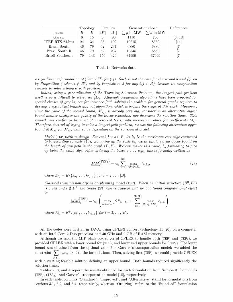
Topology Circuits Generation/Load Referencesname |B| |E| |Ω0| |Ω1|

∑g in MW

∑d in MW

Garver 6 15 6 90 1110 760 [3, 18]IEEE RTS 24-bus 24 34 38 102 10215 8560 [14]

Brazil South 46 79 62 237 6880 6880 [7]Brazil South R 46 79 62 237 10545 6880 [7]

Brazil Southeast 79 143 156 429 37999 37999 [7]

Table 1: Networks data

a tight linear reformulation of (Kirchoff1) for (ij). Such is not the case for the second bound (givenby Proposition 4 when i /∈ B0, and by Proposition 3 for any i, j ∈ B), because its computationrequires to solve a longest path problem.

Indeed, being a generalization of the Traveling Salesman Problem, the longest path problemitself is very difficult to solve, see [19]. Although polynomial algorithms have been proposed forspecial classes of graphs, see for instance [39], solving the problem for general graphs requires todevelop a specialized branch-and-cut algorithm, which is beyond the scope of this work. Moreover,since the value of the second bound, M ij, is already very big, considering an alternative biggerbound neither modifies the quality of the linear relaxation nor decreases the solution times. Thisremark was confirmed by a set of unreported tests, with increasing values for coefficients Mij.Therefore, instead of trying to solve a longest path problem, we use the following alternative upperbound MM ij for M ij, with value depending on the considered model:

Model (TEPR)with re-design: For each bus b ∈ B, let kb be the maximum-cost edge connectedto b, according to costs (16). Summing up the costs ckb we certainly get an upper bound onthe length of any path in the graph (B,E). We can reduce this value, by forbidding to pickup twice the same edge. After ordering the buses b1, . . . , b|B|, this is formally written as

MM(TEPR)ij = γij

|B|∑i=1

max(bibj)∈Ebi

cb1b2 , (23)

where Ebi = E\kb1 , . . . , kbi−1 for i = 2, . . . , |B|.

Classical transmission expansion planning model (TEP): When an initial structure (B0, E0)

is given and i /∈ B0, the bound (23) can be reduced with no additional computational effortto

MM(TEP)ij = γij

maxb1,b2∈B0

SPb1−b2 +

|B\B0|∑i=1

max(bibj)∈E1

bi

cb1b2

,

where E1bi

= E1\kb1 , . . . , kbi−1 for i = 2, . . . , |B|.

All the codes were written in JAVA, using CPLEX concert technology 11 [20], on a computerwith an Intel Core 2 Duo processor at 2.40 GHz and 2 GB of RAM memory.

Although we used the MIP black-box solver of CPLEX to handle both (TEP) and (TEPR), weprovided CPLEX with a lower bound for (TEP), and lower and upper bounds for (TEPR). The lowerbound was obtained from the optimal value t of Garvers’s transportation model: we added the

constraint∑k∈Ω1

ckxk ≥ t to the formulations. Then, solving first (TEP), we could provide CPLEX

with a starting feasible solution defining an upper bound. Both bounds reduced significantly thesolution times.

Tables 2, 3, and 4 report the results obtained for each formulation from Section 3, for models(TEP), (TEPR), and Garver’s transportation model [18], respectively.

In each table, columns “Standard”, “Improved”, and “Alternative” stand for formulations fromsections 3.1, 3.2, and 3.4, respectively, whereas “Ordering” refers to the “Standard” formulation

15

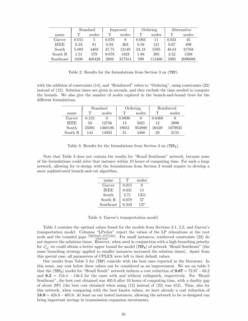
Standard Improved Ordering Alternativename T nodes T nodes T nodes T nodes

Garver 0.015 5 0.078 8 0.093 11 0.031 45IEEE 0.23 81 0.92 363 0.56 121 0.67 499South 5.085 4403 47.75 12149 24.18 5595 48.61 31768

South R 1.51 579 9.079 1823 1.88 395 3.52 1508Southeast 2438 468428 2888 317314 599 113460 5095 2096088

Table 2: Results for the formulations from Section 3 on (TEP).

with the addition of constraints (14), and “Reinforced” refers to “Ordering”, using constraints (22)instead of (12). Solution times are given in seconds, and they exclude the time needed to computethe bounds. We also give the number of nodes explored in the branch-and-bound trees for thedifferent formulations.

Standard Ordering Reinforcedname T nodes T nodes T nodes

Garver 0.124 0 0.0936 0 0.0468 0IEEE 50 12756 13 5021 12 3999South 35091 1368186 19052 952880 20438 1079935

South R 144 14933 31 4408 29 3155

Table 3: Results for the formulations from Section 3 on (TEPR).

Note that Table 3 does not contain the results for “Brazil Southeast” network, because noneof the formulations could solve that instance within 10 hours of computing time. For such a largenetwork, allowing for re-design with the formulations from Section 3 would require to develop amore sophisticated branch-and-cut algorithm.

name T nodesGarver 0.015 0IEEE 0.031 14South 2.71 1351

South R 0.078 57Southeast 0.343 137

Table 4: Garver’s transportation model.

Table 5 contains the optimal values found for the models from Sections 2.1, 2.2, and Garver’stransportation model. Columns “LPrelax” report the values of the LP relaxations at the rootnode and the rounded gaps Optimal−LPrelax

Optimal . For small instances, reinforced constraints (22) donot improve the solutions times. However, when used in conjunction with a high branching priorityfor x1

ij , we could obtain a better upper bound for model (TEPR) of network “Brazil Southeast” (thesame branching strategy applied to smaller instances increased the solution times). Apart fromthis special case, all parameters of CPLEX were left to their default values.

Our results from Table 5 for (TEP) coincide with the best ones reported in the literature. Inthis sense, any cost below these values can be considered as an improvement. We see on table 5that the (TEPR) model for “Brazil South” network induces a cost reduction of 9.67 = 72.87− 63.2and 8.2 = 154.4 − 146.2 for the cases with and without redispatch, respectively. For “BrazilSoutheast”, the best cost obtained was 405.9 after 10 hours of computing time, with a duality gapof about 29% (the best cost obtained when using (12) instead of (22) was 412). Thus, also forthis network, when comparing with the best known values, we have already a cost reduction of18.9 = 424.8− 405.9. At least on our tested instances, allowing the network to be re-designed canbring important savings in transmission expansion investments.

16

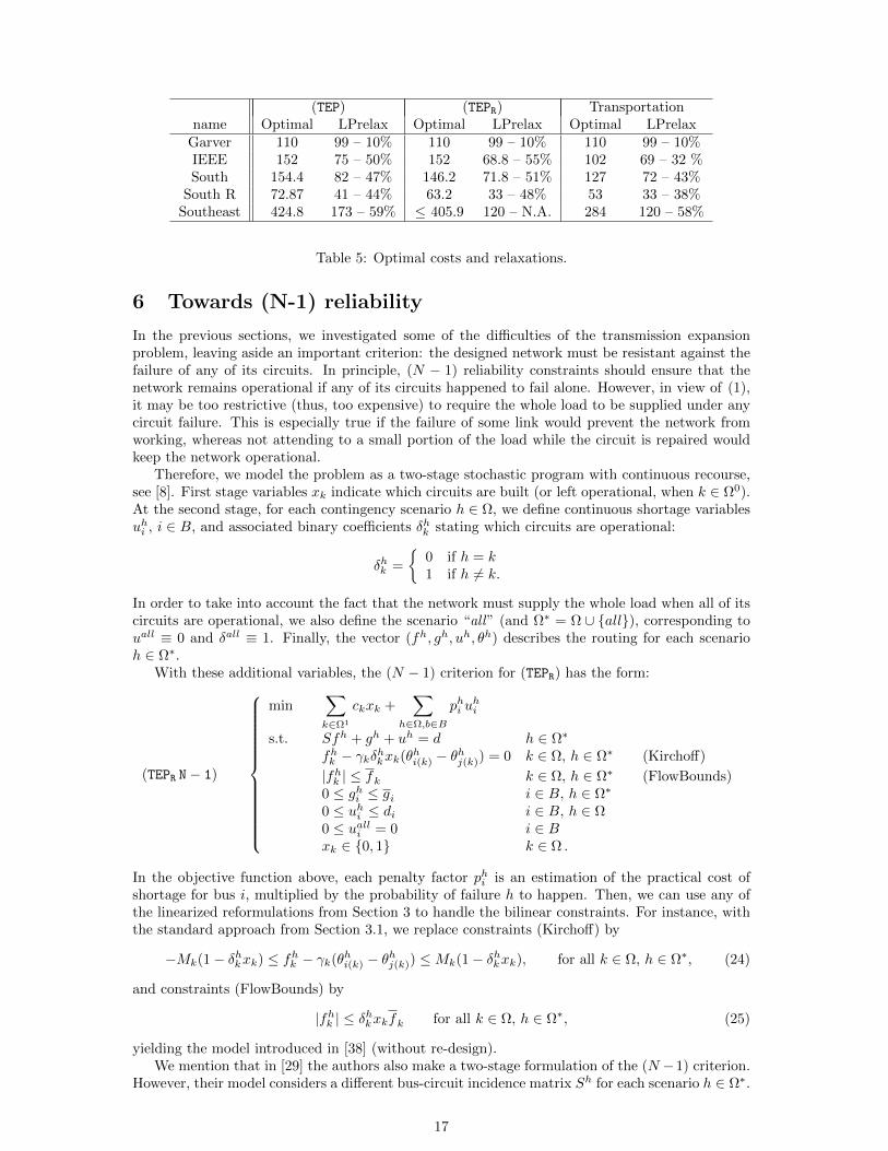
(TEP) (TEPR) Transportationname Optimal LPrelax Optimal LPrelax Optimal LPrelax

Garver 110 99 – 10% 110 99 – 10% 110 99 – 10%IEEE 152 75 – 50% 152 68.8 – 55% 102 69 – 32 %South 154.4 82 – 47% 146.2 71.8 – 51% 127 72 – 43%

South R 72.87 41 – 44% 63.2 33 – 48% 53 33 – 38%Southeast 424.8 173 – 59% ≤ 405.9 120 – N.A. 284 120 – 58%

Table 5: Optimal costs and relaxations.

6 Towards (N-1) reliability

In the previous sections, we investigated some of the difficulties of the transmission expansionproblem, leaving aside an important criterion: the designed network must be resistant against thefailure of any of its circuits. In principle, (N − 1) reliability constraints should ensure that thenetwork remains operational if any of its circuits happened to fail alone. However, in view of (1),it may be too restrictive (thus, too expensive) to require the whole load to be supplied under anycircuit failure. This is especially true if the failure of some link would prevent the network fromworking, whereas not attending to a small portion of the load while the circuit is repaired wouldkeep the network operational.

Therefore, we model the problem as a two-stage stochastic program with continuous recourse,see [8]. First stage variables xk indicate which circuits are built (or left operational, when k ∈ Ω0).At the second stage, for each contingency scenario h ∈ Ω, we define continuous shortage variablesuhi , i ∈ B, and associated binary coefficients δhk stating which circuits are operational:

δhk =

0 if h = k1 if h 6= k.

In order to take into account the fact that the network must supply the whole load when all of itscircuits are operational, we also define the scenario “all” (and Ω∗ = Ω ∪ all), corresponding touall ≡ 0 and δall ≡ 1. Finally, the vector (fh, gh, uh, θh) describes the routing for each scenarioh ∈ Ω∗.

With these additional variables, the (N − 1) criterion for (TEPR) has the form:

(TEPR N− 1)

min∑k∈Ω1

ckxk +∑

h∈Ω,b∈B

phi uhi

s.t. Sfh + gh + uh = d h ∈ Ω∗

fhk − γkδhkxk(θhi(k) − θhj(k)) = 0 k ∈ Ω, h ∈ Ω∗ (Kirchoff)

|fhk | ≤ fk k ∈ Ω, h ∈ Ω∗ (FlowBounds)0 ≤ ghi ≤ gi i ∈ B, h ∈ Ω∗

0 ≤ uhi ≤ di i ∈ B, h ∈ Ω0 ≤ ualli = 0 i ∈ Bxk ∈ 0, 1 k ∈ Ω .

In the objective function above, each penalty factor phi is an estimation of the practical cost ofshortage for bus i, multiplied by the probability of failure h to happen. Then, we can use any ofthe linearized reformulations from Section 3 to handle the bilinear constraints. For instance, withthe standard approach from Section 3.1, we replace constraints (Kirchoff) by

−Mk(1− δhkxk) ≤ fhk − γk(θhi(k) − θhj(k)) ≤Mk(1− δhkxk), for all k ∈ Ω, h ∈ Ω∗, (24)

and constraints (FlowBounds) by

|fhk | ≤ δhkxkfk for all k ∈ Ω, h ∈ Ω∗, (25)

yielding the model introduced in [38] (without re-design).We mention that in [29] the authors also make a two-stage formulation of the (N −1) criterion.

However, their model considers a different bus-circuit incidence matrix Sh for each scenario h ∈ Ω∗.

17

Such second-stage matrices are defined by suppressing in S the column related to circuit h (so thatSall = S). Our simpler recourse formulation (TEPR N − 1), with a fixed matrix S, should ease theuse of Stochastic Programming decomposition algorithms.

Model time nodes optimal LPrelaxTransportation 0.5 11 116 106.7 – 8%

(TEP N− 1) 3.8 31 118.4 106.7 – 9.8%(TEPR N− 1) 8.3 67 118.4 106.7 – 9.8%

Table 6: (N − 1) reliability constraints for Garver’s network.

We can see preliminary computational results on Table 6 for Garver’s network, using again theMIP solver of CPLEX 11. Model (TEP N − 1) stands for (TEPR N − 1) with additional constraintsxk = 1 for k ∈ Ω0, and “Transportation” for (TEPR N− 1) without (Kirchoff). Since the considerednetwork is small, there is no “slack” for the re-design model to give any improvement: the optimalvalues of (TEP N− 1) and (TEPR N− 1) are equal. For this reason, rather than giving insight on themodel with re-design, our results in Table 6 should be considered as a validation of our solvingmethodology for (TEPR N− 1).

In addition to (N−1) constraints, it is important for the expansion planning problem to consideruncertainty both in the electricity demand and generation. In this case, instead of (or in additionto) considering contigency scenarios h ∈ Ω, the 2-stage formulation (TEPR N− 1) makes use of a setW such that to each scenario ω ∈ W corresponds a demand/generation vector (d(ω), g(ω)). As in(TEPR N− 1), the design decisions x must be taken here-and-now, while the wait-and-see decisionsof recourse (f(ω), g(ω), u(ω), θ(ω)) depend on each scenario ω ∈ W. The main difference with thereliability models is that demand/generation scenarios do not need the additional vector δ, becauseuncertainty is fully characterized by the values of d(ω) and g(ω). Finally, one could consider boththe (N − 1) reliability criterion and different scenarios for demand and generation, see [29].

For networks bigger than “Garver”, solving to optimality (TEPR N− 1) or one of the extensionsevocated above needs developing efficient decomposition algorithms, an interesting subject of futureresearch.

Acknowledgements

This research is supported by an “Actions de Recherche Concertees” (ARC) projet of the “Com-munautee francaise de Belgique”. Michael Poss is a research fellow of the “Fonds pour la Formationa la Recherche dans l’Industrie et dans l’Agriculture” (FRIA). Research of Claudia Sagastizabalsupported by CNPq and FAPERJ. The authors would also like to thank a referee for constructivecomments.

References

[1] K. Abhishek, S. Leyffer, and J. T. Linderoth, Filmint: An outer-approximation-based solver fornonlinear mixed integer programs, Argonne National Laboratory, Mathematics and ComputerScience Division, Argonne, IL., 2008.

[2] R. K. Ahuja, Thomas, T. L. Magnanti, and J. B. Orlin, Network flows: Theory, algorithms,and applications, Prentice Hall, 1993.

[3] Natalia Alguacil, Alexis L. Motto, and Antonio J. Conejo, Transmission expansion planning:A mixed-integer lp approach, IEEE Transactions on Power Systems 18 (2003), no. 3, 1070–1077.

[4] L. Bahiense, G.C. Oliveira, M. Pereira, and S. Granville, A mixed integer disjunctive modelfor transmission network expansion, Power Systems, IEEE Transactions on 16 (2001), no. 3,560–565.

18

[5] D. Bienstock and S. Mattia, Using mixed-integer programming to solve power grid blackoutproblems, Discrete Optimization 4 (2007), no. 1, 115–141.

[6] S. Binato, G. C. Oliveira, and J. L.Araujo, A Greedy Randomized Adaptive Search Procedurefor Transmission Expansion Planning, IEEE Transactions on Power Systems 16 (2001), no. 2,247–253.

[7] Silvio Binato, Optimal expansion of transmission networks by benders decomposition and cut-ting planes, Ph.D. dissertation (Portuguese), Federal University of Rio de Janeiro, 2000.

[8] J. R. Birge and F. V. Louveaux, Introduction to stochastic programming (2nd edition), SpringerVerlag, New-York, 2008.

[9] M.O. Buygi, G. Balzer, H.M. Shanechi, and M. Shahidehpour, Market based transmissionexpansion planning: fuzzy risk assessment, vol. 2, April 2004, pp. 427–432 Vol.2.

[10] M.O. Buygi, H.M. Shanechi, G. Balzer, M. Shahidehpour, and N. Pariz, Network planning inunbundled power systems, Power Systems, IEEE Transactions on 21 (2006), no. 3, 1379–1387.

[11] J. Choi, T. Tran, A.A. El-Keib, R. Thomas, H. Oh, and R. Billinton, A method for transmis-sion system expansion planning considering probabilistic reliability criteria, Power Systems,IEEE Transactions on 20 (2005), no. 3, 1606–1615.

[12] Jaeseok Choi, T.D. Mount, and R.J. Thomas, Transmission expansion planning using contin-gency criteria, Power Systems, IEEE Transactions on 22 (2007), no. 4, 2249–2261.

[13] T. G. Crainic, Service network design in freight transportation, European Journal of Opera-tional Research 122 (2000), 272–288.

[14] Irenio de Jesus Silva Junior, Planejamento da expansao de sistemas de transmissao con-siderando seguranca e planos de programacao da geracao, Ph.D. dissertation (Portuguese),Universidade Estadual de Campinas, 2005.

[15] S. de la Torre, A.J. Conejo, and J. Contreras, Transmission expansion planning in electricitymarkets, Power Systems, IEEE Transactions on 23 (2008), no. 1, 238–248.

[16] E.J. deOliveira, Jr. daSilva, I.C., J.L.R. Pereira, and Jr. Carneiro, S., Transmission systemexpansion planning using a sigmoid function to handle integer investment variables, PowerSystems, IEEE Transactions on 20 (2005), no. 3, 1616–1621.

[17] Risheng Fang and D.J. Hill, A new strategy for transmission expansion in competitive elec-tricity markets, Power Systems, IEEE Transactions on 18 (2003), no. 1, 374–380.

[18] L.L. Garver, Transmission network estimation using linear programming, IEEE Trans. PowerAppar. Syst. 89 (1970), no. 7, 1688– 1697.

[19] William W. Hardgrave and George L. Nemhauser, On the relation between the traveling-salesman and the longest-path problems, Operations Research 10 (1962), no. 5, 647–657.

[20] ILOG CPLEX Division, Gentilly, France, Ilog. ilog cplex 11.0 reference manual., 2007.

[21] R. M. Karp, Reducibility among combinatorial problems, Complexity of Computer Computa-tions (R. E. Miller and J. W. Thatcher, eds.), Plenum Press, 1972, pp. 85–103.

[22] G. Latorre, R.D. Cruz, J.M. Areiza, and A. Villegas, Classification of publications and modelson transmission expansion planning, Power Systems, IEEE Transactions on 18 (2003), no. 2,938–946.

[23] J.A. Lopez, K. Ponnambalam, and V.H. Quintana, Generation and transmission expansionunder risk using stochastic programming, Power Systems, IEEE Transactions on 22 (2007),no. 3, 1369–1378.

19

[24] M. Lu, Z.Y. Dong, and T.K. Saha, A framework for transmission planning in a competitiveelectricity market, Transmission and Distribution Conference and Exhibition: Asia and Pacific,2005 IEEE/PES, 2005, pp. 1–6.

[25] P. Maghouli, S.H. Hosseini, M.O. Buygi, and M. Shahidehpour, A multi-objective frame-work for transmission expansion planning in deregulated environments, Power Systems, IEEETransactions on 24 (2009), no. 2, 1051–1061.

[26] G.L. Nemhauser and L.A. Wolsey, Integer and combinatorial optimization, Wiley, New York,1999.

[27] G. C. Oliveira, S. Binato, L. Bahiense, L. Thome, and M.V. Pereira, Security-constrainedtransmission planning: A mixed-integer disjunctive approach, Proc. IEEE/Power Eng. Soc.Transmission and Distribution Conf., Sao Paulo, Brazil, 2004.

[28] G.C. Oliveira, S. Binato, M.V.F. Pereira, and L.M. Thome, Multi-stage transmission expansionplanning considering multiple dispatches and contingency criterion, Congresso Brasileiro deAutomatica (2004).

[29] Gerson C. Oliveira, Silvio Binato, and Mario V. F. Pereira, Value-based transmission expansionplanning of hydrothermal systems under uncertainty, IEEE Transactions on power systems 622(2007), no. 4, 1429–1435.

[30] Tsamasphyrou P., Renaud A., and Carpentier P, Transmission network planning under un-certainty with benders decomposition, Lecture Notes in Economics and Mathematical Systems481 (2000), 457–472.

[31] M. Pereira and S. Granville, Analysis of the linearized power flow model in benders decom-position, Tech. Report SOL 85-04, SOL Lab, Dept. of Oper. Research, Stanford University,1985.

[32] I. Quesada and I. E. Grossman, An LP/NLP based branch and bound algorithm for convexMINLP optimization problems., Comput. Chem. Eng. 16 (1992), no. 10/11, 937–947.

[33] R. Raman and I. E. Grossmann, Modeling and computational techniques for logic based integerprogramming, Computers and Chemical Engineering 18 (1994), no. 7, 563–578.

[34] F.S. Reis, P.M.S. Carvalho, and L.A.F.M. Ferreira, Reinforcement scheduling convergence inpower systems transmission planning, Power Systems, IEEE Transactions on 20 (2005), no. 2,1151–1157.

[35] Id.J. Silva, M.J. Rider, R. Romero, and C.A.F. Murari, Transmission network expansionplanning considering uncertainty in demand, Power Systems, IEEE Transactions on 21 (2006),no. 4, 1565–1573.

[36] K. Singh, A. Philpott, and K. Wood, Column-generation for design of survivable networks,Working paper, 2008.

[37] O.B. Tor, A.N. Guven, and M. Shahidehpour, Congestion-driven transmission planning con-sidering the impact of generator expansion, Power Systems, IEEE Transactions on 23 (2008),no. 2, 781–789.

[38] P. Tsamasphyrou, A. Renaud, and P. Carpentier, Transmission network planning: An efficientBenders decomposition scheme, 13th PSCC in Trondheim, 1999.

[39] R. Uehara Y. Uno, On computing longest paths in small graph classes, International Journalof Foundations of Computer Science 18 (2007), no. 5, 911–930.

[40] R. Villanasa, Transmission network planning using linear and mixed linear integer program-ming, Ph.D. thesis, Ressenlaer Polythechnic Institute, 1984.

[41] R. T. Wong, A dual ascent approach for Steiner tree problems on a directed graph, Mathemat-ical Programming 28 (1984), no. 3, 271–287.

20

[42] D. Yuan, An annotated bibliography in communication network design and routing, Ph.D.thesis, Institute of Technology, Linkopings Universitet, 2001.

[43] Jun Hua Zhao, Zhao Yang Dong, P. Lindsay, and Kit Po Wong, Flexible transmission expan-sion planning with uncertainties in an electricity market, Power Systems, IEEE Transactionson 24 (2009), no. 1, 479–488.

21