arX

iv:1

001.

2010

v5 [

astr

o-ph

.EP

] 24

Sep

201

4

Transits and Occultations

Joshua N. WinnMassachusetts Institute of Technology

When we are fortunate enough to view an exoplanetary system nearly edge-on, the star and planetperiodically eclipse each other. Observations of eclipses—transits and occultations—provide a bonanzaof information that cannot be obtained from radial-velocity data alone, such as the relative dimensionsof the planet and its host star, as well as the orientation of the planet’s orbit relative to the sky plane andrelative to the stellar rotation axis. The wavelength-dependence of the eclipse signal gives clues about thethe temperature and composition of the planetary atmosphere. Anomalies in the timing or other propertiesof the eclipses may betray the presence of additional planets or moons. Searching for eclipses is also aproductive means of discovering new planets. This chapter reviews the basic geometry and physics ofeclipses, and summarizes the knowledge that has been gainedthrough eclipse observations, as well as theinformation that might be gained in the future.

1. INTRODUCTION

From immemorial antiquity, men have dreamed of aroyal road to success—leading directly and easily to somegoal that could be reached otherwise only by long ap-proaches and with weary toil. Times beyond number, thisdream has proved to be a delusion.... Nevertheless, thereare ways of approach to unknown territory which lead sur-prisingly far, and repay their followers richly. There isprobably no better example of this than eclipses of heav-enly bodies.— Henry Norris Russell (1948)

Vast expanses of scientific territory have been traversedby exploiting the occasions when one astronomical bodyshadows another. The timing of the eclipses of Jupiter’smoons gave the first accurate measure of the speed of light.Observing the passage of Venus across the disk of the Sunprovided a highly refined estimate of the astronomical unit.Studying solar eclipses led to the discovery of helium, therecognition that Earth’s rotation is slowing down due totides, and the confirmation of Einstein’s prediction for thegravitational deflection of light. The analysis of eclipsingbinary stars—the subject Russell had in mind—enabled aprecise understanding of stellar structure and evolution.

Continuing in this tradition, eclipses are the “royal road”of exoplanetary science. We can learn intimate details aboutexoplanets and their parent stars through observations oftheir combined light, without the weary toil of spatially re-solving the planet and the star (see Figure 1). This chaptershows how eclipse observations are used to gain knowledgeof the planet’s orbit, mass, radius, temperature, and atmo-spheric constituents, along with other details that are other-wise hidden. This knowledge, in turn, gives clues about theprocesses of planet formation and evolution and provides alarger context for understanding the properties of the solarsystem.

An eclipseis the obscuration of one celestial body by an-other. When the bodies have very unequal sizes, the passageof the smaller body in front of the larger body is atransit

and the passage of the smaller body behind the larger bodyis anoccultation. Formally, transits are cases when the fulldisk of the smaller body passes completely within that ofthe larger body, and occultations refer to the complete con-cealment of the smaller body. We will allow those terms toinclude thegrazingcases in which the bodies’ silhouettesdo not overlap completely. Please be aware that the exo-planet literature often refers to occultations assecondaryeclipses(a more general term that does not connote an ex-treme size ratio), or by the neologisms “secondary transit”and “anti-transit.”

This chapter is organized as follows. Section 2 de-scribes the geometry of eclipses and provides the founda-tional equations, building on the discussion of Keplerian or-bits in the chapter by Murray and Correia. Readers seekinga more elementary treatment involving only circular orbitsmay prefer to start by reading Sackett (1999). Section 3 dis-cusses many scientific applications of eclipse data, includ-ing the determination of the mass and radius of the planet.Section 4 is a primer on observing the apparent decline instellar brightness during eclipses (thephotometricsignal).Section 5 reviews some recent scientific accomplishments,and Section 6 offers some thoughts on future prospects.

2. ECLIPSE BASICS

2.1 Geometry of eclipses

Consider a planet of radiusRp and massMp orbiting astar of radiusR⋆ and massM⋆. The ratioRp/R⋆ occursfrequently enough to deserve its own symbol, for which wewill usek, in deference to the literature on eclipsing binarystars. As in the chapter by Murray and Correia, we choosea coordinate system centered on the star, with the sky intheX–Y plane and the+Z axis pointing at the observer(see Figure 2). Since the orientation of the line of nodesrelative to celestial north (or any other externally definedaxis) is usually unknown and of limited interest, we might

1

Flux

Time

transit

occultation

star alone

star + planet dayside

star + planet nightside

star – planet shadow

Fig. 1.— Illustration of transits and occultations. Only the combined flux of the star and planet is observed. During a transit, the fluxdrops because the planet blocks a fraction of the starlight.Then the flux rises as the planet’s dayside comes into view. The flux dropsagain when the planet is occulted by the star.

as well align theX axis with the line of nodes; we place thedescending node of the planet’s orbit along the+X axis,givingΩ = 180.

The distance between the star and planet is given byequation (20) of the chapter by Murray and Correia:

r =a(1− e2)

1 + e cos f, (1)

wherea is the semimajor axis of the relative orbit andfis the true anomaly, an implicit function of time dependingon the orbital eccentricitye and periodP (see Section 3 ofthe chapter by Murray and Correia). This can be resolvedinto Cartesian coordinates using equations (53-55) of thechapter by Murray and Correia, withΩ = 180:

X = −r cos(ω + f), (2)

Y = −r sin(ω + f) cos i, (3)

Z = r sin(ω + f) sin i. (4)

If eclipses occur, they do so whenrsky ≡√X2 + Y 2 is

a local minimum. Using equations (2-3),

rsky =a(1 − e2)

1 + e cos f

√

1− sin2(ω + f) sin2 i. (5)

Minimizing this expression leads to lengthy algebra (Kip-ping 2008). However, an excellent approximation that wewill use throughout this chapter is that eclipses are centered

aroundconjunctions, which are defined by the conditionX = 0 and may beinferior (planet in front) orsuperior(star in front). This gives

ftra = +π

2− ω, focc = −π

2− ω, (6)

where here and elsewhere in this chapter, “tra” refers totransits and “occ” to occultations. This approximation isvalid for all cases except extremely eccentric and close-inorbits with grazing eclipses.

The impact parameterb is the sky-projected distance atconjunction, in units of the stellar radius:

btra =a cos i

R⋆

(

1− e2

1 + e sinω

)

, (7)

bocc =a cos i

R⋆

(

1− e2

1− e sinω

)

. (8)

For the common caseR⋆ ≪ a, the planet’s path across(or behind) the stellar disk is approximately a straight linebetween the pointsX = ±R⋆

√1− b2 atY = bR⋆.

2.2 Probability of eclipses

Eclipses are seen only by privileged observers who viewa planet’s orbit nearly edge-on. As the planet orbits its star,its shadow describes a cone that sweeps out a band on thecelestial sphere, as illustrated in Figure 3. A distant ob-server within the shadow band will see transits. The open-ing angle of the cone,Θ, satisfies the conditionsinΘ =

2

Fig. 2.— Illustration of a transit, showing the coordinate system discussed in Section 2.1, the four contact points and the quantitiesTandτ defined in Section 2.3, and the idealized light curve discussed in Section 2.4.

(R⋆ + Rp)/r wherer is the instantaneous star-planet dis-tance. This cone is called thepenumbra. There is also an in-terior cone, theantumbra, defined bysinΘ = (R⋆−Rp)/r,inside of which the transits are full (non-grazing).

A common situation is thate andω are known andi isunknown, as when a planet is discovered via the Dopplermethod (see chapter by Lovis and Fischer) but no informa-tion is available about eclipses. With reference to Figure 3,the observer’s celestial longitude is specified byω, but thelatitude is unknown. The transit probability is calculatedasthe shadowed fraction of the line of longitude, or more sim-ply from the requirement|b| < 1+ k, using equations (7-8)and the knowledge thatcos i is uniformly distributed for arandomly-placed observer. Similar logic applies to occulta-tions, leading to the results

ptra =

(

R⋆ ±Rp

a

)(

1 + e sinω

1− e2

)

, (9)

pocc =

(

R⋆ ±Rp

a

)(

1− e sinω

1− e2

)

, (10)

where the “+” sign allows grazing eclipses and the “−”sign excludes them. It is worth committing to memory theresults for the limiting caseRp ≪ R⋆ ande = 0:

ptra = pocc =R⋆

a≈ 0.005

(

R⋆

R⊙

)

( a

1 AU

)−1

. (11)

For a circular orbit, transits and occultations always go to-gether, but for an eccentric orbit it is possible to see transitswithout occultations or vice versa.

In other situations, one may want to marginalize overall possible values ofω, as when forecasting the expectednumber of transiting planets to be found in a survey (seeSection 4.1) or other statistical calculations. Here, one cancalculate the solid angle of the entire shadow band and di-vide by4π, or average equations (9-10) overω, giving

ptra = pocc =

(

R⋆ ±Rp

a

)(

1

1− e2

)

. (12)

Suppose you want to find a transiting planet at a particu-lar orbital distance around a star of a given radius. If a frac-tion η of stars have such planets, you must search at leastN ≈ (η ptra)

−1 stars before expecting to find a transitingplanet. A sample of>200η−1 Sun-like stars is needed tofind a transiting planet at 1 AU. Close-in giant planets havean orbital distance of approximately 0.05 AU andη ≈ 0.01,givingN >103 stars. In practice, many other factors affectthe survey requirements, such as measurement precision,time sampling, and the need for spectroscopic follow-upobservations (see Section 4.1).

2.3 Duration of eclipses

In a non-grazing eclipse, the stellar and planetary disks

3

Fig. 3.— Calculation of the transit probability.Left.—Transits are visible by observers within the penumbra of the planet, a cone withopening angleΘ with sinΘ = (R⋆+Rp)/r, wherer is the instantaneous star-planet distance.Right.—Close-up showing the penumbra(thick lines) as well as the antumbra (thin lines) within which the transits are full, as opposed to grazing.

are tangent at fourcontact timestI–tIV, illustrated in Fig-ure 2. (In a grazing eclipse, second and third contact donot occur.) Thetotal duration isTtot = tIV − tI, thefull duration isTfull = tIII − tII, the ingressduration isτing = tII − tI, and theegressduration isτegr = tIV − tIII.

Given a set of orbital parameters, the various eclipse du-rations can be calculated by setting equation (5) equal toR⋆ ± Rp to find the true anomaly at the times of contact,and then integrating equation (44) of the chapter by Murrayand Correia, e.g.,

tIII − tII =P

2π√1− e2

∫ fIII

fII

[

r(f)

a

]2

df. (13)

For a circular orbit, some useful results are

Ttot ≡ tIV − tI =P

πsin−1

[

R⋆

a

√

(1 + k)2 − b2

sin i

]

, (14)

Tfull ≡ tIII − tII =P

πsin−1

[

R⋆

a

√

(1 − k)2 − b2

sin i

]

.

(15)For eccentric orbits, good approximations are obtained bymultiplying equations (14-15) by

X(fc) [e = 0]

X(fc)=

√1− e2

1± e sinω, (16)

a dimensionless factor to account for the altered speed ofthe planet at conjunction. Here, “+” refers to transits and“−” to occultations. One must also computeb using theeccentricity-dependent equations (7-8).

For an eccentric orbit,τing andτegr are generally unequalbecause the projected speed of the planet varies between

ingress and egress. In practice the difference is slight; toleading order inR⋆/a ande,

τe − τiτe + τi

∼ e cosω

(

R⋆

a

)3(

1− b2)3/2

, (17)

which is<10−2 e for a close-in planet withR⋆/a = 0.2,and even smaller for more distant planets. For this reasonwe will use a single symbolτ to represent either the ingressor egress duration. Another important timescale isT ≡Ttot − τ , the interval between the halfway points of ingressand egress (sometimes referred to as contact times 1.5 and3.5).

In the limits e → 0, Rp ≪ R⋆ ≪ a, andb ≪ 1 − k(which excludes near-grazing events), the results are greatlysimplified:

T ≈ T0

√

1− b2, τ ≈ Tok√1− b2

, (18)

whereT0 is the characteristic time scale

T0 ≡ R⋆P

πa≈ 13 hr

(

P

1 yr

)1/3 (ρ⋆ρ⊙

)−1/3

. (19)

For eccentric orbits, the additional factor given by equa-tion (16) should be applied. Note that in deriving equa-tion (19), we used Kepler’s third law and the approximationMp ≪ M⋆ to rewrite the expression in terms of the stel-lar mean densityρ⋆. This is a hint that eclipse observationsgive a direct measure ofρ⋆, a point that is made more ex-plicit in Section 3.1.

2.4 Loss of light during eclipses

The combined fluxF (t) of a planet and star is plottedin Figure 1. During a transit, the flux drops because the

4

planet blocks a fraction of the starlight. Then the flux risesas the planet’s dayside comes into view. The flux dropsagain when the planet is occulted by the star. Conceptuallywe may dissectF (t) as

F (t) = F⋆(t)+Fp(t)−

k2αtra(t)F⋆(t) transits,

0 outside eclipses,

αocc(t)Fp(t) occultations.(20)

whereF⋆, Fp are the fluxes from the stellar and planetarydisks, and theα’s are dimensionless functions of order unitydepending on the overlap area between the stellar and plan-etary disks. In generalF⋆ may vary in time due to flares,rotation of star spots and plages, rotation of the tidal bulgeraised by the planet, or other reasons, but for simplicity ofdiscussion we take it to be a constant. In that case, only theratio f(t) ≡ F (t)/F⋆ is of interest. If we letIp andI⋆ bethe disk-averaged intensities of the planet and star, respec-tively, thenFp/F⋆ = k2Ip/I⋆ and

f(t) = 1 + k2Ip(t)

I⋆−

k2αtra(t) transits,

0 outside eclipses,

k2Ip(t)I⋆

αocc(t) occultations.(21)

Time variations inIp are caused by the changing illumi-nated fraction of the planetary disk (itsphase function), aswell as any changes intrinsic to the planetary atmosphere.To the extent thatIp is constant over the relatively shorttimespan of a single eclipse, all of the observed time vari-ation is from theα functions. As a starting approximationtheα’s are trapezoids, andf(t) is specified by the depthδ,durationT , ingress or egress durationτ , and time of con-junctiontc, as shown in Figure 2. For transits the maximumloss of light is

δtra ≈ k2[

1− Ip(ttra)

I⋆

]

, (22)

and in the usual case when the light from the planetarynightside is negligible,δtra ≈ k2. For occultations,

δocc ≈ k2Ip(tocc)

I⋆. (23)

In the trapezoidal approximation the flux variation dur-ing ingress and egress is linear in time. In reality this isnot true, partly because of the nonuniform motion of thestellar and planetary disks. More importantly, even withuniform motion the overlap area between the disks is not alinear function of time [see equation (1) of Mandel & Agol(2002)]. In addition, the bottom of a transit light curve isnot flat because real stellar disks do not have uniform inten-sity, as explained in the next section.

2.5 Limb darkening

Real stellar disks are brighter in the middle and fainterat the edge (the limb), a phenomenon known aslimb dark-ening. This causes the flux decline during a transit to be

larger thank2 when the planet is near the center of the star,and smaller thank2 when the planet is near the limb. Theeffect on the light curve is to round off the bottom and blurthe 2nd and 3rd contact points, as shown in Figure 4. Limbdarkening is a consequence of variations in temperature andopacity with altitude in the stellar atmosphere. The sight-line to the limb follows a highly oblique path into the stel-lar atmosphere, and therefore an optical depth of unity isreached at a higher altitude, where the temperature is coolerand the radiation is less intense. The resulting intensity pro-file I(X,Y ) is often described with a fitting formula suchas

I ∝ 1− u1(1 − µ)− u2(1− µ)2, (24)

whereµ ≡√1−X2 − Y 2 andu1, u2 are constant co-

efficients that may be calculated from stellar-atmospheremodels or measured from a sufficiently precise transit lightcurve. The decision to use the quadratic function of equa-tion (24) or another of the various limb-darkening “laws”(better described as fitting formulas) is somewhat arbi-trary. Claret (2004) provides a compilation of theoreticalcoefficients, and advocates a four-parameter law. South-worth (2008) investigates the results of fitting the same dataset with different limb-darkening laws. Mandel & Agol(2002) give accurate expressions forαtra(t) for some limb-darkening laws, and Gimenez (2006) shows how to com-puteαtra(t) for an arbitrary law based on earlier work byKopal (1979).

By using one of these methods to calculate the flux ofa limb-darkened disk with a circular obstruction, it is usu-ally possible to model real transit light curves to within themeasurement errors (see Section 4.3). In principle, calcu-lations of occultation light curves should take the planetarylimb darkening into account, though the precision of cur-rent data has not justified this level of detail. Likewise, inexceptional cases it may be necessary to allow for depar-tures from circular shapes, due to rotational or tidal defor-mation (see Section 6). Modelers of eclipsing binary starshave long needed to take into account these and other subtleeffects (Kallrath & Milone 2009, Hilditch 2001).

More generally, the loss of light depends on the intensityof the particular patch of the photosphere that is hidden bythe planet. The planet provides a raster scan of the stellarintensity across the transit chord. In this manner, star spotsand plages can be detected through the flux anomalies thatare observed when the planet covers them. (An example isgiven in the top right panel of Figure 8.) Even spots that arenot along the transit chord can produce observable effects,by causing variations inF⋆ and thereby causingδtra to varyfrom transit to transit.

3. SCIENCE FROM ECLIPSES

3.1 Determining absolute dimensions

Chief among the reasons to observe transits is to de-termine the mass and radius of the planet. Ideally one

5

Fig. 4.— Transits of the giant planet HD 209458b observed atwavelengths ranging from 0.32µm (bottom) to 0.97µm (top). Atshorter wavelengths, the limb darkening of the star is more pro-nounced, and the bottom of the light curve is more rounded. Thedata were collected with theHubble Space Telescopeby Knutsonet al. (2007a).

would like to know the mass in kilograms, and the radiusin kilometers, to allow for physical modeling and compar-isons with solar system planets. With only a transit lightcurve, this is impossible. The light curve by itself revealsthe planet-to-star radius ratiok ≡ Rp/R⋆ ≈

√δ but not

the planetary radius, and says nothing about the planetarymass.

To learn the planetary mass, in addition to the light curveone needs the radial-velocity orbit of the host star, andin particular the velocity semiamplitudeK⋆. Using equa-tion (66) of the chapter by Murray and Correia, and Kepler’sthird law, we may write

Mp

(Mp +M⋆)2/3=

K⋆

√1− e2

sin i

(

P

2πG

)1/3

. (25)

The observation of transits ensuressin i ≈ 1, and therebybreaks the usualMp sin i degeneracy. However, the plan-etary mass still cannot be determined independently of thestellar mass. In the usual limitMp ≪ M⋆, the data deter-

mineMp/M2/3⋆ but notMp itself.

To determine the absolute dimensions of the planet, onemust supplement the transit photometry and radial-velocityorbit with some external information about the star. De-pending on the star, the available information may includeits luminosity, spectral type, and spectrally-derived photo-spheric properties (effective temperature, surface gravity,and metallicity). A typical approach is to seek consistencybetween those data and stellar-evolutionary models, whichrelate the observable properties to the stellar mass, radius,composition, and age. In special cases it may also be pos-sible to pin down the stellar properties using interferometry(Baines et al. 2009), asteroseismology (Stello et al. 2009),or an eclipsing companion star.

Besidesδ, the transit light curve offers the observablesTtot andTfull (or T andτ ), which can be used to solve forthe impact parameterb and thescaled stellar radiusR⋆/a.For non-grazing transits, in the limitRp ≪ R⋆ ≪ a wemay invert equations (14-15) to obtain the approximate for-mulas

b2 =(1 −

√δ)2 − (Tfull/Ttot)

2(1 +√δ)2

1− (Tfull/Ttot)2(26)

R⋆

a=

π

2δ1/4

√

T 2tot − T 2

full

P

(

1 + e sinω√1− e2

)

. (27)

If in addition τ ≪ T , such as is the case for small planetson non-grazing trajectories, the results are simplified stillfurther to

b2 = 1−√δT

τ, (28)

R⋆

a=

π

δ1/4

√Tτ

P

(

1 + e sinω√1− e2

)

. (29)

The orbital inclinationi may then be obtained using equa-tion (7). These approximations are useful for theoreticalcalculations and for developing an intuition about how the

6

system parameters affect the observable light curve. Forexample,R⋆/a controls the product ofT and τ while bcontrols their ratio. However, as mentioned earlier, for fit-ting actual data one needs a realistic limb-darkened model,linked to a Keplerian orbital model.

The dimensionless ratiosR⋆/a and Rp/a are impor-tant for several reasons: (i) They set the scale of tidal in-teractions between the star and planet. (ii)Rp/a deter-mines what fraction of the stellar luminosity impinges onthe planet, as discussed in Section 3.4. (iii)R⋆/a can beused to determine a particular combination of the stellarmean densityρ⋆ and planetary mean densityρp:

ρ⋆ + k3ρp =3π

GP 2

(

a

R⋆

)3

. (30)

This can be derived from Kepler’s third law (Seager &Mallen-Ornelas 2003). Sincek3 is usually small, the sec-ond term on the left side of equation (30) is often negligibleandρ⋆ can be determined purely from transit photometry.

This method for estimatingρ⋆ has proven to be a usefuldiagnostic in photometric transit surveys: a true transit sig-nal should yield a value ofρ⋆ that is consistent with expec-tations for a star of the given luminosity and spectral type.Furthermore, once a precise light curve is available,ρ⋆ is avaluable additional constraint on the stellar properties.

Interestingly, it is possible to derive the planetary surfacegravitygp ≡ GMp/R

2p independently of the stellar proper-

ties:

gp =2π

P

√1− e2 K⋆

(Rp/a)2 sin i. (31)

This is derived from equation (66) of the chapter by Murrayand Correia and Kepler’s third law (Southworth et al. 2007).

In short, precise transit photometry and Doppler ve-locimetry lead to correspondingly precise values of the stel-lar mean densityρ⋆ and planetary surface gravitygp. How-ever, the errors inMp andRp are ultimately limited by theuncertainties in the stellar properties.

3.2 Timing of eclipses

The orbital periodP can be determined by timing a se-quence of transits, or a sequence of occultations, and fittinga linear function

tc[n] = tc[0] + nP, (32)

wheretc[n] is the time of conjunction of thenth event. Thetimes must first be corrected to account for the Earth’s or-bital motion and consequent variations in the light traveltime. When comparing transit and occultation times, onemust further correct for the light travel time across the line-of-sight dimension of the planetary orbit. As long as there isno ambiguity inn, the error inP varies inversely as the to-tal number of eclipses spanned by the observations, makingit possible to achieve extraordinary precision inP .

If the orbit does not follow a fixed ellipse—due to forcesfrom additional bodies, tidal or rotational bulges, general

relativity, or other non-Keplerian effects—then there willbe variations in the interval between successive transits,aswell as the interval between transits and occultations andthe shape of the transit light curve. These variations maybe gradual parameter changes due to precession (Miralda-Escude 2002), or short-term variations due to other planets(Holman & Murray 2005, Agol et al. 2005) or moons (Kip-ping 2009). The effects can be especially large for bodiesin resonant orbits with the transiting planet. By monitoringtransits one might hope to detect such bodies, as discussedin the chapter by Fabrycky.

When transits and occultations are both seen, a power-ful constraint on the shape of the orbit is available. For acircular orbit, those events are separated in time byP/2,but more generally the time interval depends one andω.To first order ine, integratingdt/df between conjunctionsgives

∆tc ≈P

2

[

1 +4

πe cosω

]

. (33)

In this case, the timing of transits and occultations gives anestimate ofe cosω. Likewise the relative durations of thetransit and the occultation depend on the complementaryparametere sinω,

Tocc

Ttra≈ 1 + e sinω

1− e sinω. (34)

Sterne (1940) and de Kort (1954) give the lengthy exact re-sults for arbitrarye andi. Because the uncertainty in∆tc/Pis typically smaller than that inTtra/Tocc (by a factor ofP/T ), the eclipse data constraine cosω more powerfullythane sinω.

The resulting bounds one are often valuable. For exam-ple, planets on close-in eccentric orbits are internally heatedby the friction that accompanies the time-variable tidal dis-tortion of the planet. Empirical constraints one therebyhelp to understand the thermal structure of close-in planets.For more distant planets, bounds one are helpful in the sta-tistical analysis of exoplanetary orbits. As described in thechapter by Cumming and in Part V of this volume, the ob-served eccentricity distribution of planetary orbits is a clueabout the processes of planet formation and subsequent or-bital evolution.

Eclipse-based measurements ofttra, tocc, andP are al-most always more precise than those based on spectroscopicor astrometric orbital data. The eclipse-based results cangreatly enhance the analysis of those other data. For ex-ample, the usual radial-velocity curve has 6 parameters, butif ttra, tocc, andP are known from eclipses, the number offree parameters is effectively reduced to 3, thereby boostingthe achievable precision in the other 3 parameters.

3.3 Transmission spectroscopy

We have been implicitly assuming that the planetary sil-houette has a sharp edge, but in reality the edge is fuzzy. Forgas giant planets there is no well-defined surface, and even

7

planets with solid surfaces may have thick atmospheres.During a transit, a small portion of the starlight will be fil-tered through the upper atmosphere of the planet, where it isonly partially absorbed. The absorption will be wavelength-dependent due to the scattering properties of atoms andmolecules in the planetary atmosphere. At the wavelengthof a strong atomic or molecular transition, the atmosphere ismore opaque, and the planet’s effective silhouette is larger.This raises the prospect of measuring thetransmission spec-trum of the planet’s upper atmosphere and thereby gainingknowledge of its composition.

To calculate the expected signal one must follow the ra-diative transfer of the incident starlight along a grazing tra-jectory through the planet’s stratified atmosphere. The cal-culation is rather complicated (see, e.g., Seager & Sasselov2000, Brown 2001) but the order of magnitude of the effectis easily appreciated. For a strong transition, the effectivesize of the planet grows by a few atmospheric scale heightsH , where

H =kBT

µmg(35)

andT is the temperature,µm is the mean molecular mass,g is the local gravitational acceleration, andkB is Boltz-mann’s constant. DefiningRp as the radius within whichthe planet is optically thick at all wavelengths, the extra ab-sorption due to the optically thin portion of the atmospherecauses the transit depth to increase by

∆δ =π(Rp +NHH)2

πR2⋆

−πR2

p

πR2⋆

≈ 2NHδ

(

H

Rp

)

, (36)

whereNH , the number of scale heights, is of order unity.The signal is most readily detectable for planets with largeH : low surface gravity, low mean molecular mass, and hightemperature. For a “hot Jupiter” around a Sun-like star (δ =0.01, T ≈ 1300 K, g ≈ 25 m s−2, µm = 2 amu) the signalis ∆δ ∼ 10−4. For an Earth-like planet around a Sun-likestar (δ = 10−4, T ≈ 273 K, g ≈ 10 m s−2, µm = 28 amu),the signal is∆δ ∼ 10−6.

The signal can be detected by observing a transit lightcurve at multiple wavelengths, using different filters or aspectrograph. One then fits a limb-darkened light-curvemodel to the time series obtained at each wavelength, re-quiring agreement in the orbital parameters and allowing avalue ofδ specific to each wavelength. The resulting vari-ations inδ(λ) are expected to be of the order of magnitudegiven by equation (36). It is best to gather all of the dataat the same time, because intrinsic stellar variability is alsochromatic.

3.4 Occultation spectroscopy

As discussed in Section 2.4, when the planet is com-pletely hidden the starlight declines by a fractionδocc =k2Ip/I⋆, wherek is the planet-to-star radius ratio andIp/I⋆is the ratio of disk-averaged intensities. Observations span-ning occultations thereby reveal the relative brightness of

the planetary disk, ifk is already known from transit obser-vations. The planetary radiation arises from two sources:thermal radiation and reflected starlight. Because the planetis colder than the star, the thermal component emerges atlonger wavelengths than the reflected component.

For the moment we suppose that the planet is of uni-form brightness, and that the observing wavelength is longenough for thermal emission to dominate. Approximatingthe planet and star as blackbody radiators,

δocc(λ) = k2Bλ(Tp)

Bλ(T⋆)−→ k2

Tp

T⋆(37)

whereBλ(T ) is the Planck function,

Bλ(T ) ≡2hc2

λ5

1

ehc/(λkBT ) − 1−→ 2ckBT

λ4, (38)

in which T is the temperature,λ is the wavelength,h isPlanck’s constant, andc is the speed of light. The limitingcases are for the “Rayleigh-Jeans” limitλ ≫ hc/(kBT ).The decrementδocc that is observed by a given instrumentis obtained by integrating equation (37) over the bandpass.

Even when the planetary radiation is not described by thePlanck law, one may define abrightness temperatureTb(λ)as the equivalent blackbody temperature that would lead tothe observed value ofδocc(λ). The brightness temperatureis sometimes a convenient way to describe the wavelength-dependent intensity even when it is not thermal in origin.

There may be departures from a blackbody spectrum—spectral features—discernible in the variation of brightnesstemperature with wavelength. In contrast with transmissionspectroscopy, which refers to starlight that grazes the plane-tary limb (terminator), here we are referring to the emissionspectrum of the planet averaged over the visible disk of thedayside. Occultation spectroscopy and transit spectroscopythereby provide different and complementary informationabout the planetary atmosphere.

It is possible to measure the reflectance spectrum of theplanet’s dayside by observing at shorter wavelengths, or ac-curately subtracting the thermal emission. The occultationdepth due to reflected light alone is

δocc(λ) = Aλ

(

Rp

a

)2

, (39)

whereAλ is thegeometric albedo, defined as the flux re-flected by the planet when viewed at opposition (full phase),divided by the flux that would be reflected by a flat and per-fectly diffusing surface with the same cross-sectional areaas the planet. One of the greatest uncertainties in atmo-spheric modeling is the existence, prevalence, and compo-sition of clouds. Since clouds can produce very large albedovariations, reflectance spectroscopy may help to understandthe role of clouds in exoplanetary atmospheres.

For a close-in giant planet, the reflectance signal is∼10−4 while for an Earthlike planet at 1 AU it is∼10−9.The detection prospects are better for closer-in planets.

8

However, the closest-in planets are also the hottest, andtheir radiation may be dominated by thermal emission. An-other consideration is that planets withT > 1500 K are ex-pected to be so hot that all potentially cloud-forming con-densable materials are in gaseous form. The theoreticallypredicted albedos are very low, of order10−3, due to strongabsorption by neutral sodium and potassium.

Real planets do not have uniformly bright disks. Gaseousplanets are limb darkened or brightened, and may havelatitudinal zones with high contrast, like Jupiter. Rockyplanets may have surface features and oceans. To the ex-tent that departures from uniform brightness could be de-tected, occultation data would provide information on thespatially-resolved planetary dayside. Specifically, the lightcurve of the ingress or egress of an occultation gives aone-dimensional cumulative brightness distribution of theplanet.

3.5 The Rossiter-McLaughlin effect

In addition to the spectral variations induced by the plan-etary atmosphere, there are spectral variations arising fromthe spatial variation of the stellar spectrum across the stellardisk. The most pronounced of these effects is due to stel-lar rotation: light from the approaching half of the stellardisk is blueshifted, and light from the receding half is red-shifted. Outside of transits, rotation broadens the spectrallines but does not produce an overall Doppler shift in thedisk-integrated starlight. However, when the planet coverspart of the blueshifted half of the stellar disk, the integratedstarlight appears slightly redshifted, and vice versa.

Thus, the transit produces a time-variable spectral dis-tortion that is usually manifested as an “anomalous” radialvelocity, i.e., a Doppler shift that is greater or smaller thanthe shift expected from only the star’s orbital motion. Fig-ure 5 illustrates this effect. It is known as the Rossiter-McLaughlin (RM) effect, after the two astronomers whomade the first definitive observations of this kind for binarystars, in 1924.

The maximum amplitude of the anomalous radial veloc-ity is approximately

∆VRM ≈ k2√

1− b2(v⋆ sin i⋆), (40)

where v⋆ sin i⋆ is the line-of-sight component of thestellar equatorial rotation velocity. For a Sun-like star(v⋆ sin i⋆=2 km s−1), the maximum amplitude is∼20 m s−1

for a Jovian planet and∼0.2 m s−1 for a terrestrial planet.This amplitude may be comparable to (or even larger than)the amplitude of the spectroscopic orbit of the host star.Furthermore it is easier to maintain the stability of a spec-trograph over the single night of a transit than the longerduration of the orbital period. Hence the RM effect is aneffective means of detecting and confirming transits, pro-viding an alternative to photometric detection.

In addition, by monitoring the anomalous Doppler shiftthroughout a transit, it is possible to measure the angle on

the sky between the planetary orbital axis and the stellarrotation axis. Figure 6 shows three trajectories of a transit-ing planet that have the same impact parameter, and henceproduce identical light curves, but that have different ori-entations relative to the stellar spin axis, and hence pro-duce different RM signals. The signal for a well-alignedplanet is antisymmetric about the midtransit time (left pan-els), whereas a strongly misaligned planet that blocks onlythe receding half of the star will produce only an anomalousblueshift (right panels).

A limitation of this technique is that it is only sensitiveto the angle between thesky projectionsof the spin and or-bital angular momentum vectors. The true angle betweenthose vectors is usually poorly constrained becausei⋆ is un-known. Nevertheless it may be possible to tell whether theplanetary orbit is prograde or retrograde, with respect to thedirection of stellar rotation. It is also possible to combineresults from different systems to gain statistical knowledgeabout spin-orbit alignment.

More broadly, just as transit photometry provides a rasterscan of the intensity of the stellar photosphere along thetransit chord, RM data provide a raster scan of the line-of-sight velocity field of the photosphere. This gives an inde-pendent measure of the projected rotation ratev⋆ sin i⋆, andreveals the velocity structure of starspots or other featuresthat may exist on the photosphere.

4. OBSERVING ECLIPSES

4.1 Discovering eclipsing systems

Figure 7 shows the rate of exoplanet discoveries over thelast 20 years, highlighting the subset of planets known totransit. Transits have been discovered in two ways. Oneway is to find the planet in a Doppler survey (see chap-ter by Lovis and Fischer), and then check for transits bymonitoring the brightness of the star throughout the inferiorconjunction. This was the path to discovery for 6 of the 64known systems, including the first example, HD 209458b(Charbonneau et al. 2000, Henry et al. 2000, Mazeh etal. 2000). The probability that transits will occur is givenby equation (9) and the times of inferior conjunction can becalculated from the parameters of the spectroscopic orbit(Kane 2007).

The other way is to conduct photometric surveillance ofstars that are not yet known to have any planets, an idea dat-ing back to Struve (1952). As an illustration let us considerthe requirements for a program to discover hot Jupiters. Asdiscussed in Section 2.2, a bare minimum of103 Sun-likestars must be examined to find a transiting planet with anorbital distance of0.05 AU. The observations must be pre-cise enough to detect a 1% flux drop, and must extend forat least several times longer than the 3 day orbital period.The difficulty increases dramatically for smaller planets inwider orbits: in an idealized survey of nearby field starslimited by photon noise (see Section 4.2) the sensitivity to

9

Fig. 5.— Illustration of the Rossiter-McLaughlin (RM) effect. The three columns show three successive phases of a transit. Thefirst row shows the stellar disk, with the grayscale representing the projected rotation velocity: the approaching limbis black and thereceding limb is white. The second row shows the corresponding stellar absorption line profiles, assuming rotation to bethe dominantbroadening mechanism. The “bump” occurs because the planethides a fraction of the light that contributes a particular velocity to theline-broadening kernel. The third row shows the case for which other line-broadening mechanisms are important; here the RM effect ismanifested only as an “anomalous Doppler shift.” Adapted from Gaudi & Winn (2007).

Fig. 6.— Using the RM effect to measure the angleλ between the sky projections of the orbital and stellar-rotational axes. Threedifferent possible trajectories of a transiting planet areshown, along with the corresponding RM signal. The trajectories all have thesame impact parameter and produce the same light curve, but they differ inλ and produce different RM curves. The dotted lines are forthe case of no limb darkening, and the solid lines include limb darkening. From Gaudi & Winn (2007).

10

Year of Discovery Announcement

0

20

40

60

80

Num

ber

of E

xopl

anet

s

89 90 91 92 93 94 95 96 97 98 99 00 01 02 03 04 05 06 07 08 09

All exoplanetsTransiting exoplanets

Fig. 7.— Rate of exoplanet discovery. The light bars show thenumber of announcements of newly discovered planets, and the dark barsshow the subset of transiting planets. Compiled with data from exoplanet.eu, an encyclopedic web site maintained by J. Schneider.

transiting planets scales approximately asR6p/P

5/3 (Gaudi2005; Gaudi, Seager, & Mallen-Ornelas 2005). More real-istic calculations take into account the spread in radius andluminosity among the surveyed stars, the duration and time-sampling of observations, the appropriate threshold valueofthe signal-to-noise ratio, and other factors (see, e.g., Pepperet al. 2003, Beatty & Gaudi 2008).

Photometric surveys are much less efficient than Dopplersurveys, in the sense that only a small fraction of plan-ets transit, and even when transits occur they are under-way only a small fraction of the time. On the other hand,the starting equipment for a photometric survey is mod-est, consisting in some cases of amateur-grade telescopesor telephoto lenses and cameras, whereas Doppler surveysrequire upfront a large telescope and sophisticated spectro-graph. For these reasons the royal road of eclipses enticedmany astronomers to embark on photometric transit sur-veys. More than a dozen surveys were undertaken, includ-ing a few longitudinally-distributed networks to providemore continuous time coverage. Major efforts were madeto automate the observations, and to develop algorithms forprecise wide-field photometry (Tamuz et al. 2005, Kovacset al. 2005) and transit detection (Kovacs et al. 2002).Horne (2003) took stock of all the ongoing and plannedsurveys, and ventured to predict a bounty of 10–100 newplanets per month, in an article subtitled “Hot Jupiters Ga-lore.”

The royal road turned out to have some potholes. Oneobstacle was the high rate of “false positives,” signals thatresemble planetary transits but are actually grazing eclipsesof a binary star, or an unresolved combination of an eclips-ing binary star and a third star. In the latter case, the deepeclipses of the binary star are diluted to planet-like propor-tions by the constant light of the third star. In some surveys

the false positives outnumbered the planets by 10 to 1. Rul-ing them out required spectroscopy with large telescopes,which became the bottleneck in the discovery process (see,e.g., O’Donovan et al. 2007). Another obstacle was corre-lated noise (“red noise”) in the survey photometry (see Sec-tion 4.3). Pont et al. (2006) showed that red noise slashedthe sensitivity of the search algorithms, thereby providing aquantitative solution to the “Horne problem” of why tran-siting planets were not being found as rapidly as expected.

Only a few of the surveyors were able to overcome theseobstacles. The 5 most successful surveys were OGLE,which used a 1 m telescope to survey 14-16th magnitudestars; and the TrES, XO, HAT, and SuperWASP surveys,which used≈0.1 m lenses to survey 10-12th magnitudestars. Many of today’s transiting planets are named afterthese surveys: for more details see Udalski et al. (2002),Alonso et al. (2004), McCullough et al. (2005), Bakos etal. (2007), and Pollacco et al. (2006). The OGLE planetswere found first, although the brighter stars from the wider-field surveys were far more amenable to false-positive re-jection and detailed characterization.

On the other end of the cost spectrum are photometricsurveys performed from space. By avoiding the deleteriouseffects of the Earth’s atmosphere, it is possible to beat theprecision of ground-based observations (see Section 4.2).It is also possible to avoid the usual interruptions due tothe vagaries of the weather, and even to avoid the day-nightcycle if the spacecraft is in an orbit far from Earth. Thetwo ongoing space-based missionsCoRoTandKepler aredescribed in Sections 5.1 and 6, respectively.

One space-based survey that did not discover any plan-ets neverthless produced an interesting result. Gillilandetal. (2000) used theHubble Space Telescopeto seek close-ingiant planets in the globular cluster 47 Tucanae. No transits

11

were found, even though 17 were expected based on thesurvey characteristics and the observed frequency of close-in giant planets around nearby field stars. The absence ofclose-in planets could be due to the crowded stellar envi-ronment (which could inhibit planet formation or disruptplanetary systems) or the cluster’s low metallicity (whichhas been found to be correlated with fewer planets in theDoppler surveys; see the chapters by Lovis and Fischerand by Cumming). The null results of a subsequent sur-vey of the less-crowded outskirts of 47 Tucanae suggest thatcrowding is not the primary issue (Weldrake et al. 2005).

4.2 Measuring the photometric signal

Even after a transiting planet is discovered, it takes acareful hand to measure the transit signal precisely enoughto achieve the scientific goals set forth in Section 3. The lossof light is only 1% for a Sun-like star crossed by a Jupiter-sized planet, and 0.01% for an Earth-sized planet. Occul-tations produce still smaller signals. This is the domain ofprecise time-series differential photometry. The term “dif-ferential” applies because only the fractional variationsareof interest, as opposed to the actual intensity in Janskys orother standardized units. Eclipses can also be detected viaspectroscopy (Section 3.5) or polarimetry (Carciofi & Ma-galhaes 2005) but here we focus on the photometric signal,with emphasis on ground-based optical observations.

First you must know when to observe. To observe aneclipse requires a triple coincidence: the eclipse must behappening, the star must be above the horizon, and the Sunmust be down. Transit times can be predicted based on asequence of previously measured transit times, by fittingand extrapolating a straight line (equation 32). Occultationtimes can also be predicted from a listing of transit times,but are subject to additional uncertainty due to the depen-dence one andω (equation 33).

Next you should monitor the flux of the target star alongwith other nearby stars of comparable brightness. The mea-sured fluxes are affected by short-term variations in atmo-spheric transparency, as well as the gradual change in theeffective atmospheric path length (theairmass) as the starrises and sets. However, the ratios of the fluxes betweennearby stars are less affected. As long as some of the com-parison stars are constant in brightness then the relative fluxof the target star can be tracked precisely.

This task is usually accomplished with a charge-coupleddevice (CCD) imaging camera and software for calibrat-ing the images, estimating the sky background level, andcounting the photons received from each star in excess ofthe sky level (aperture photometry). Howell (1999) ex-plains the basic principles of CCDs and aperture photom-etry. For more details on differential aperture photome-try using an ensemble of comparison stars, see Gilliland &Brown (1988), Kjeldsen & Frandsen (1992), and Everett &Howell (2001). In short, the fluxes of the comparison starsare combined, and the flux of the target star is divided bythe comparison signal, giving a time series of relative flux

measurements spanning the eclipse with as little noise aspossible. For bright stars observed at optical wavelengths,among the important noise sources are photon noise, scintil-lation noise, differential extinction, and flat-fielding errors,which we now discuss in turn.

Photon noiserefers to the unavoidable fluctuations in thesignal due to the quantization of light. It is also calledPois-son noisebecause the photon count rate obeys a Poissondistribution. If a star deliversN photons s−1 on average,then the standard deviation in the relative flux due to photonnoise is approximately(N∆t)−1/2 for an exposure lasting∆t seconds. This noise source affects the target and com-parison stars independently. The sky background also in-troduces Poisson noise, which can be troublesome for faintstars or infrared wavelengths. The photon noise in the com-parison signal can be reduced by using many bright com-parison stars. Beyond that, improvement is possible only bycollecting more photons, using a bigger telescope, a moreefficient detector, or a wider bandpass.

Scintillationis caused by fluctuations in the index of re-fraction of air. The more familiar term is “twinkling.” Forintegration times∆t >∼ 1 s, the standard deviation in the rel-ative flux due to scintillation is expected to scale with tele-scope diameterD, observatory altitudeh, integration time,and airmass as

σscin = σ0(Airmass)7/4

D2/3(∆t)1/2exp

(

− h

8000 m

)

, (41)

based on a theory of atmospheric turbulence by Reiger (1963),with empirical support from Young (1967) and others. Thecoefficientσ0 is often taken to be 0.064 whenD is ex-pressed in centimeters and∆t in seconds, but this must beunderstood to be approximate and dependent on the localmeteorology. Scintillation affects both the target and com-parison stars, although for closely-spaced stars the vari-ations are correlated (Ryan & Sandler 1998). One alsoexpects scintillation noise to decrease with wavelength.Thus, scintillation noise is reduced by employing a largetelescope (or combining results from multiple small tele-scopes), choosing nearby comparison stars, and observingat a long wavelength from a good site.

Differential extinctionis used here as a shorthand for“second-order color-dependent differential extinction.” Tofirst order, if two stars are observed simultaneously, theirfluxes are attenuated by the Earth’s atmosphere by the samefactor and the flux ratio is preserved. To second order, thebluer star is attenuated more, because scattering and ab-sorption are more important at shorter wavelengths. Thiseffect causes the flux ratio to vary with airmass as well aswith short-term transparency fluctuations. It can be reducedby choosing comparison stars bracketing the target star incolor, or using a narrow bandpass. The advantage of a nar-row bandpass must be weighed against the increased photonnoise.

Flat fieldingis the attempt to correct for nonuniform illu-mination of the detector and pixel-to-pixel sensitivity varia-tions, usually by dividing the images by a calibration image

12

of a uniformly-lit field. If the stars were kept on the samepixels throughout an observation, then flat-fielding errorswould not affect the flux ratios. In reality the light from agiven star is detected on different pixels at different times,due to pointing errors, focus variations, and seeing varia-tions. Imperfect flat fielding coupled with these variationsproduce noise in the light curve. The impact of flat-fieldingerrors is reduced by ensuring the calibration images havenegligible photon noise, maintaining a consistent pointing,and defocusing the telescope. Defocusing averages downthe interpixel variations, reduces the impact of seeing vari-ations, and allows for longer exposure times without sat-uration, thereby increasing the fraction of the time spentcollecting photons as opposed to resetting the detector. De-focusing is good for what ails you, as long as the stars donot blend together.

This discussion of noise sources is not exhaustive; it is inthe nature of noise that no such listing can be complete. Forexample, the gain of the detector may drift with temper-ature, or scattered moonlight may complicate backgroundsubtraction. A general principle is to strive to keep every-thing about the equipment and the images as consistent aspossible. Another good practice is to spend at least as muchtime observing the star before and after the eclipse as duringthe eclipse, to establish the baseline signal and to character-ize the noise.

It is often advisable to use a long-wavelength bandpass,not only to minimize scintillation and differential extinc-tion, but also to reduce the effects of stellar limb darken-ing on the transit light curve. The degree of limb darken-ing diminishes with wavelength because the ratio betweenblackbody spectra of different temperatures is a decreas-ing function of wavelength. Transit light curves observedat longer wavelengths are “boxier,” with sharper cornersand flatter bottoms. All other things being equal, this re-duces the statistical uncertainties in the transit parameters,but other factors should also be considered. For example, atinfrared wavelengths, limb darkening may be small, but thesky background is bright and variable.

The space-based observer need not worry about scintil-lation and differential extinction, and enjoys a low back-ground level even at infrared wavelengths. Extremely pre-cise photometry is possible, limited only by the size ofthe telescope and the degree to which the detector is well-calibrated. With theHubble Space Telescopea precision ofapproximately10−4 per minute-long integration has beenachieved, a few times better than the best ground-basedlight curves. Figure 8 allows for some side-by-side com-parisons of ground-based and space-based data. However,going to space is not a panacea. When unforeseen calibra-tion issues arise after launch, they are difficult to resolve. Inlow Earth orbit, there are also unhelpful interruptions dueto occultations by the Earth, as well as problems with scat-tered Earthshine and cosmic rays. More remote orbits offersuperior observing conditions, but require greater effortandexpense to reach.

Fig. 8.— Examples of transit light curves based on ground-basedobservations (left) and space-based observations (right). In the topright panel, the “bump” observed just before midtransit is inter-preted as the covering of a dark starspot by the planet. From upperleft to lower right, the references are Winn et al. (2007a), Rabuset al. (2009), Winn et al. (2007b), Pont et al. (2008), Holmanetal. in prep., Gillon et al. (2007), Winn et al. (2008), and Carter etal. (2009).

13

4.3 Interpreting the photometric signal

Once you have an eclipse light curve, the task remainsto derive the basic parametersδ, T, τ, tc and their uncer-tainties, as well as the results for other quantities such asgpandρ⋆ that can be derived from those parameters. The an-alytic equations given in Section 2 for the eclipse duration,timing, and other properties are rarely used to analyze data.Rather, a parametric model is fitted to the data, based onthe numerical integration of Kepler’s equation to calculatethe relative positions of the star and planet, as well as oneof the prescriptions mentioned in Section 2.4 for computingthe loss of light from the limb-darkened stellar photosphere.

The first task is writing a code that calculates the lightcurve of the star-planet system as a function of the orbitalparameters and eclipse parameters. Then, this code is usedin conjunction with one of many standard routines to op-timize the parameter values, typically by minimizing thesum-of-squares statistic,

χ2 =

N∑

i=1

[

fi(obs)− fi(calc)

σi

]2

, (42)

where fi(obs) is the observed value of relative flux attime ti, fi(calc) is the calculated flux (depending on themodel parameters), andσi is the measurement uncertainty.The techniques found in standard works such as NumericalRecipes (Press et al. 2007) are applicable here, although afew points of elaboration are warranted for the specific con-text of eclipse photometry.

It is common to adopt a Bayesian attitude, in which theparameters are viewed as random variables whose probabil-ity distributions (“posteriors”) are constrained by the data.This can be done in a convenient and elegant fashion us-ing the Monte Carlo Markov Chain (MCMC) method, inwhich a chain of points is created in parameter space usinga few simple rules that ensure the collection of points willconverge toward the desired posterior. This method givesthe full multidimensional joint probability distributionforall the parameters, rather than merely giving individual er-ror bars, making it easy to visualize any fitting degeneraciesand to compute posteriors for any combination of parame-ters that may be of interest. Although a complete MCMCbriefing is beyond the scope of this chapter, the interestedreader should consult the textbook by Gregory (2005) aswell as case studies such as Holman et al. (2006), CollierCameron et al. (2007), and Burke et al. (2007).

A vexing problem is the presence of correlated noise,as mentioned in Section 4.2. The use of equation (42) isbased on the premise that the measurement errors are sta-tistically independent. In many cases this is plainly false.Real light curves have bumps, wiggles, and slopes span-ning many data points. These can be attributed to differen-tial extinction, flat-fielding errors, or astrophysical effectssuch as starspots. Thus the number of truly independentsamples is smaller than the number of data points, and thepower to constrain model parameters is correspondingly re-

duced. Ignoring the correlations leads to false precision inthe derived parameters, but accounting for correlations isnot straightforward and can be computationally intensive.Some suggestions are given by Pont et al. (2006) and Carter& Winn (2009a).

The treatment of stellar limb darkening presents anotherunwelcome opportunity to underestimate the parameter un-certainties. It is tempting to adopt one of the standard limb-darkening laws (see Section 2.5) and hold the coefficientsfixed at values deemed appropriate for the host star, basedon stellar-atmosphere models. However, with precise datait is preferable to fit for the coefficients, or at least to allowfor some uncertainty in the atmospheric models. In thosefew cases where the data have been precise enough to testthe models, the models have missed the mark (Claret 2009).

Although fitting data is a job for a computer, it is never-theless useful to have analytic formulas for the achievableprecision in the eclipse parameters. The formulas are handyfor planning observations, and for order-of-magnitude esti-mates of the observability (or not) of effects such as vari-ations in transit times and durations. The formulas givenhere are based on the assumptions that the data have uni-form time sampling∆t, and independent Gaussian errorsσin the relative flux. A useful figure of merit isQ ≡

√Nδ/σ,

whereδ is the transit depth andN is the number of datapoints obtained during the transit. A Fisher informationanalysis (essentially a glorified error propagation) leadstoestimates for the 1σ uncertainties in the transit parameters(Carter et al. 2008):

σδ ≈ Q−1δ, (43)

σtc ≈ Q−1T√

τ/2T , (44)

σT ≈ Q−1T√

2τ/T , (45)

στ ≈ Q−1T√

6τ/T , (46)

which are valid whenδ ≪ 1, limb darkening is weak, andthe out-of-transit flux is known precisely. In this case,σtc <σT < στ . Correlated errors and limb darkening cause theseformulas to be underestimates.

5. SUMMARY OF RECENT ACHIEVEMENTS

5.1 Discoveries of transiting planets

Discoveries of exoplanets, and transiting exoplanets inparticular, have abounded in recent years (Figure 7). Asof December 2009, approximately 64 transiting planets areknown, representing 15% of the total number of exoplanetsdiscovered. Figure 9 shows their masses, radii, and orbitalperiods. It is important to remember that these planets arenot a randomly selected subset of exoplanets. The proper-ties of the ensemble have been shaped by powerful selectioneffects in the surveys that led to their discovery, favoringlarge planets in short-period orbits.

Despite these selection effects, the known transitingplanets exhibit a striking diversity. They span three or-ders of magnitude in mass, and one order of magnitude in

14

1 10 100 1000Mass [MEarth]

1

10

Rad

ius

[RE

arth]

0.0 0.5 1.0 1.5 2.0Mass [MJup]

0.0

0.5

1.0

1.5

2.0

Rad

ius

[RJu

p]

1 10 100Orbital Period [days]

1

10

100

1000

Mas

s [M

Ear

th]

1 2 3 4 5Orbital Period [days]

0.0

0.5

1.0

1.5

2.0

Mas

s [M

Jup]

Fig. 9.— Masses, radii, and orbital periods of the transiting exoplanets.Upper left: Radius versus mass, on logarithmic scales. Thedotted lines are loci of constant mean density (0.5, 1, and 2 gcm−3, from top to bottom).Upper right: Same, but on linear scales, andwith the axes restricted to highlight the gas giants that dominate the sample.Lower left: Mass versus orbital period, on a logarithmicscale. The two long-period outliers are HD 17156b (P = 21 d) and HD 80606b (P = 111 d). Lower right: Same, but on a linear scale,and with axes restricted to highlight the gas giants. The anticorrelation between mass and orbital period is evident.

15

radius. Most are gas giants, comparable in mass and radiusto Jupiter. There are also two planets with sizes more likeNeptune and Uranus, as well as two even smaller planetswith sizes only a few times larger than Earth, a categorythat has come to be known as “super-Earths.”

The two transiting super-Earths (Figure 10) were foundwith completely different strategies. TheCoRoT(COnvec-tion, ROtation, and planetary Transits) team uses a satelliteequipped with a 0.27 m telescope and CCD cameras to ex-amine fields of∼10,000 stars for a few months at a time,seeking relatively short-period planets (P . 20 d). Alongwith several giant planets they have found a planet of radius1.7R⊕ in a 20-hour orbit around a G dwarf star, producinga transit depth of only3.4× 10−4 (Leger et al. 2009). Thisis smaller than the detection threshold of any of the ground-based surveys, demonstrating the advantage of space-basedphotometry. However, it proved difficult to spectroscopi-cally confirm that the signal is indeed due to a planet, be-cause the host star is relatively faint and chromosphericallyactive (Queloz et al. 2009).

Another project, called MEarth (and pronouncedmirth),seeks transits of small planets from the ground by focusingon very small stars (M dwarfs), for which even a super-Earth would produce a transit depth of order 1%. Becausesuch stars are intrinsically faint, one must search the wholesky to find examples bright enough for follow-up work.That is why MEarth abandoned the usual survey concept inwhich many stars are monitored within a single telescope’sfield of view. Instead they monitor M dwarf stars one ata time, using several 0.4 m telescopes. Using this strategythey found a planet of radius2.7 R⊕ in a 1.6-day periodaround a star of radius0.21 R⊙ (Charbonneau et al. 2009).The large transit depth of 1.3% invites follow-up observa-tions to study the planet’s atmosphere.

At the other extreme, several transiting objects havemasses greater than 10MJup, reviving the old debate aboutwhat should and should not be considered a planet. Theradii of these massive objects are not much larger thanJupiter’s radius, in agreement with predictions that be-tween about 1–50MJup the pressure due to Coulomb forces(which would giveR ∝ M1/3) and electron degener-acy pressure (R ∝ M−1/3) conspire to mute the mass-dependence of the radius.

Almost all of the transiting planets have short orbital pe-riods (<10 days), due to the decline in transit probabilitywith orbital distance (equation 12). Two conspicuous ex-ceptions are HD 17156b withP = 21 days (Barbieri etal. 2009), and HD 80606b withP = 111 days (Moutouet al. 2009, Garcia-Melendo & McCullough 2009, Fosseyet al. 2009). Both of those planets were discovered by theDoppler method and found to transit through photometricfollow-up observations. They were recognized as high-priority targets because both systems have highly eccentricorbits oriented in such a way as to enhance the probabilityof eclipses. Thus despite their long orbital periods, theirpe-riastron distances are small (<0.1 AU) along with all of theother known transiting planets.

5.2 Follow-up photometry and absolute dimensions

Follow-up observations of transits have allowed the ba-sic transit parametersδ, T, τ to be determined to within1% or better, and absolute dimensions of planets to withinabout 5%. Compilations of system parameters are given byTorres, Winn, & Holman (2008) and Southworth (2009).The orbital periods are known with 8 significant digitsin some cases. Ground-based observations have achieveda photometric precision of 250 ppm per 1 min sample,through the techniques described in Section 4.2.

A pathbreaking achievement was theHubble Space Tele-scopelight curve of HD 209458 by Brown et al. (2001),with a time sampling of 80 s and a precision of 110 ppm,without the need for comparison stars. With theSpitzerSpace Telescopethe photon noise is generally higher, butthere are compensatory advantages: there is little limb-darkening at at mid-infrared wavelengths, and uninter-rupted views of entire events are possible because the satel-lite is not in a low-earth orbit. Among the most spectaculardata yet obtained in this field was the 33 hr observation byKnutson et al. (2007b) of the K star HD 189733, spanningboth a transit and occultation of its giant planet. The datawere gathered withSpitzerat a wavelength of 8µm, andare shown in Figure 11. They not only provided extremelyprecise light curves of the transit and occultation, but alsoshowed that the combined flux rises gradually in betweenthose two events, demonstrating that the dayside is hotterthan the nightside.

Among the properties of the close-in giant planets, a fewpatterns have emerged. The planetary mass is inversely re-lated to the orbital period (Mazeh, Zucker, & Pont 2005).This anticorrelation has been variously attributed to selec-tion effects, tidal interactions, and thermal evaporationofthe planetary atmosphere. There is also a positive correla-tion between the metallicity of the host star and the inferred“core mass” of the planet (Guillot et al. 2006), by whichis meant the mass of heavy elements required in models ofthe planetary interior that agree with the observed mass andradius. It is tempting to interpret this latter correlationassupport for the core-accretion theory of planet formation.

A persistent theme in this field, and a source of contro-versy and speculation, is that several of the transiting giantplanets have radii that are 10-50% larger than expected frommodels of hydrogen-helium planets, even after accountingfor the intense stellar heating and selection effects (see thechapter by Correia and Laskar). Among the possible ex-planations for these “bloated” planets are tidal heating (see,e.g., Miller et al. 2009); unknown atmospheric constituentsthat efficiently trap internal heat (Burrows et al. 2007); en-hanced downward convection allowing the incident stellarradiation to reach significant depth (Guillot & Showman2002); and inhibition of convection within the planet thattraps internal heat (Chabrier & Baraffe 2007).

Likewise, a few planets are observed to besmallerthan expected for a hydrogen-helium planet with the ob-served mass and degree of irradiation. Some examples are

16

Fig. 10.— Transits of two different super-Earths, GJ 1214b (left) and CoRoT-7b (right). The planets are approximately the same size,but because GJ 1214b orbits a small star (spectral type M4.5V) its transit depth is much larger than that of CoRoT-7b, which orbits alarger star (G9V). References: Charbonneau et al. (2009), Leger et al. (2009).

Fig. 11.— The combined 8µm brightness of the K star HD 189733 and its giant planet, overa 33 hr interval including a transit and anoccultation. The bottom panel shows the same data as the top panel but with a restricted vertical scale to highlight the gradual rise inbrightness as the planet’s dayside comes into view. The amplitude of this variation gives the temperature contrast between the dayside(estimated as1211 ± 11 K) and the nightside (973± 33 K). From Knutson et al. (2007b).

17

HD 149026b (Sato et al. 2005) and HAT-P-3b (Torres etal. 2007). The favored interpretation is that these planetsare enriched in elements heavier than hydrogen and helium,and the increased mean molecular weight leads to a largeroverall density. Some degree of enrichment might be ex-pected because Jupiter and Saturn are themselves enrichedin hevay elements relative to the Sun. However the twoplanets just mentioned would need to be enriched still fur-ther; in the case of HD 149026b, theoretical models suggestthat the planet is 65% heavy elements by mass.

5.3 Atmospheric physics

Atmospheric spectra have been obtained for several gasgiant planets, especially the two “hot Jupiters” with thebrightest host stars, HD 209458b and HD 189733b. Bothtransmission and emission spectroscopy have been under-taken, mainly with the space telescopesHubbleandSpitzer.Figures 12 and 13 show examples of both transmission(transit) and emission (occultation) spectra. These obser-vations have stimulated much theoretical work on exoplan-etary atmospheres (see the chapters by Chambers and byD’Angelo et al. for more details than are presented here).

This enterprise began with the optical detection of neu-tral sodium in a transmission spectrum of HD 209458b byCharbonneau et al. (2002). For that same planet, Vidal-Madjar et al. (2003) measured an enormous transit depthof (15 ± 4)% within an ultraviolet bandpass bracketingthe wavelength of the Lyman-α transition, which they at-tributed to neutral hydrogen gas being blown off the planet.For HD 189733b, a rise in transit depth toward shorterwavelengths was observed by Pont et al. (2007) and inter-preted as Rayleigh scattering in the planet’s upper atmo-sphere.

Recent attention has turned to infrared wavelengths,where molecules make their imprint. In the emission spec-tra, departures from a blackbody spectrum have been inter-preted as arising from water, methane, carbon monoxide,and carbon dioxide (see, e.g., Grillmair et al. 2008, Swainet al. 2009). Absorption features in transmission spectrahave been interpreted as arising from water and methane(see, e.g., Swain et al. 2008, Tinetti et al. 2007).

Despite these impressive achievements, many issues re-garding the atmospheres of hot Jupiters remain unsettled.Controversies arise because spectral features are observedwith a low signal-to-noise ratio and are not always repro-ducible, as illustrated in Figure 12. This is understand-able, as the observers have pushed the instruments beyondtheir design specifications to make these demanding mea-surements. In addition, the theoretical interpretation ofthespectra is in a primitive state. A published spectrum isusually accompanied by a model that fits the data, but leftunanswered are whether the model is unique and how well-constrained are its parameters. Recent work by Madhusud-han & Seager (2009) addresses this problem.

One theme that has arisen in the last few years is thatsome hot Jupiters have aninversion layerin their upper at-

mospheres, within which the temperature rises with heightinstead of the usual decline. The evidence for an inver-sion layer is emission in excess of a blackbody spectrumbetween 4–8µm, where excessabsorptionwas expecteddue to water vapor. The interpretation is that water is seenin emission because it exists in a hot, tenuous stratosphere.

Hot stratospheres develop when starlight is strongly ab-sorbed by some species at low pressure (at high altitude)where the atmosphere does not radiate efficiently. Theidentity of this absorber in hot Jupiter atmospheres hasbeen a topic of debate. Gaseous titanium oxide and vana-dium oxide are candidates (Hubeny et al. 2003), as arephotochemically-produced sulfur compounds (Zahnle etal. 2009). Meanwhile observers are searching for corre-lations between the presence or absence of an inversionlayer, the degree of stellar irradiation, the magnitude ofthe day-night temperature difference, and other observableproperties.

A few of the known planets have highly eccentric or-bits and small periastron distances, and are therefore sub-ject to highly variable stellar irradiation. Observers havemonitored the planetary thermal emission following perias-tron passages, to gauge the amplitude and timescale of thethermal response to stellar heating. In the most extremecase, Laughlin et al. (2009) watched the effective tempera-ture of the giant planet HD 80606b rise from about 800 Kto 1500 K after periastron passage, and inferred that thecharacteristic radiative timescale of the upper atmosphereis about 4.5 hr.

Although the thermal emission from hot Jupiters hasbeen detected in many cases, at infrared and optical wave-lengths, there has been no unambiguous detection ofstarlightreflectedfrom the planetary atmosphere. The bestresulting upper limit on the visual planetary albedo is 0.17(with 3σ confidence), for the case of HD 209458b (Roweet al. 2008). This rules out highly reflective clouds of thesort that give Jupiter its visual albedo of 0.5. However, thelimits have not been of great interest to the theorists, whopredicted all along that the visual albedos of hot Jupiterswould be very small.

5.4 Tidal evolution and migration

Almost all of the known transiting planets are closeenough to their parent stars for tidal effects to be impor-tant. The tidal bulges on the star and planet provide “han-dles” for the bodies to torque each other, and tidal frictionslowly drains energy from the system (see the chapter byFabrycky). For a typical hot Jupiter, the sequence of eventsis expected to be as follows: (i) Over∼106 yr, the planet’srotational period is synchronized with its orbital period,andits obliquity (the angle between its rotational and orbitalangular momentum vectors) is driven to zero. (ii) Over∼109 yr, the orbit is circularized. (iii) After∼1012 yr (i.e.not yet), the stellar rotational period is synchronized withthe orbital period, the stellar obliquity is driven to zero,andthe orbit decays, leading to the engulfment of the planet.

18

Fig. 12.— Transmission (transit) spectroscopy of the gas giant HD 189733b, using theHubble Space Telescope. The symbols witherrors bars are measurements of the effective planet-to-star radius ratio as a function of wavelength. The dip at 1.6µm was interpretedas evidence for water, and the rise at 2.1µm as evidence for methane (Swain et al. 2008). However, subsequent observations at 1.7µmand 1.9µm, shown with darker symbols and gray bands, disagree with the earlier results and are consistent with a Rayleigh scatteringmodel (solid and dashed curves). From Sing et al. (2009).

Fig. 13.— Occultation spectroscopy of the gas giant HD 189733b, using theSpitzer Space Telescope. The points show measurements ofthe flux density ratio of the planet and star as a function of wavelength. The smaller and finer-sampled points are based on observationswith a dispersive spectrograph while the larger points are based on broadband filter photometry. The three lines show theoutputs ofmodel atmospheres with varying choices for the parametersPn, specifying the efficiency of heat transfer from dayside to nightside, andκe, specifying the opacity of a putative high-altitude absorbing species. From Grillmair et al. (2008).

19

The timescales for these processes are highly uncertain, andmore complex histories are possible if there are additionalplanets in the system or if the planet’s internal structure isstrongly affected by tidal heating.

Tidal circularization is implicated by the fact that plan-ets with orbital periods shorter than∼10 days tend tohave smaller orbital eccentricities than longer-period plan-ets. This fact was already known from Doppler surveys,but for eclipsing planets the eccentricities can be measuredmore precisely (see Section 3.2). It is possible that the“bloating” of some of the close-in giant planets (Section5.3) is related to the heat that was produced during the cir-cularization process, or that may still be ongoing.

As for tidal synchronization, observations withSpitzerhave revealed planets with a cold side facing away from thestar and a hot side facing the star (see Figure 11). This couldbe interpreted as evidence for synchronization, although itis not definitive, because it is also possible that the heat fromthe star is re-radiated too quickly for advection to homoge-nize the upper atmosphere of the planet.

Tidal decay of the orbit would be observable as a grad-ual decline in the orbital period (Sasselov 2003). For mostsystems the theoretical timescale for tidal decay is muchlonger than the age of the star, and indeed no evidence forthis process has been found. However in at least one case(WASP-18b; Hellier et al. 2009) the theoretical timescalefor tidal decay is muchshorter than the stellar age, becauseof the large planetary mass and short orbital period. Theexistence of this system suggests that the theoretical expec-tations were wrong and dissipation is slower in reality.

Likewise, in most cases one would not expect thatenough time has elapsed for tides to modify the star’s spinrate or orientation (Barker & Ogilvie 2009). This suggeststhat the measurements of the projected spin-orbit angle us-ing the RM effect (Section 3.5) should be interpreted in thecontext of planet formation and evolution rather than tides.A close spin-orbit alignment is expected because a star andits planets inherit their angular momentum from a commonsource: the protostellar disk. However, for hot Jupitersthere is the complication that they presumably formed atlarger distances and “migrated” inward through processesthat are poorly understood. Some of the migration theo-ries predict that the original spin-orbit alignment shouldbe preserved, while others predict occasionally large mis-alignments. For example, tidal interactions with the pro-toplanetary disk (see chapter by Showman et al.) shoulddrive the system into close alignment (Marzari & Nelson2009), while planet-planet scattering or Kozai oscillationswith tidal friction (see chapter by Fabrycky) should resultin misaligned systems.

The projected spin-orbit angle has been measured forabout 20 exoplanets, all of them close-in giants. Some ex-amples of data are shown in Figure 14. In many cases theresults are consistent with good alignment, with measure-ment precisions ranging from 1–20 (for a recent summary,see Fabrycky & Winn 2009). However there are now atleast 4 clear cases of misaligned systems. One such case is

XO-3b, a massive planet in a close-in eccentric orbit that istilted by more than 30 with respect to the stellar equator(Hebrard et al. 2008, Winn et al. 2009a). Even more dra-matic is HAT-P-7b, for which the planetary orbit and stellarspin axis are tilted by more than86 (Winn et al. 2009b,Narita et al. 2009). The planetary orbit is either polar (go-ing over the north and south poles of the star) or retrograde(revolving in the opposite direction as the star is rotating).Another possible retrograde system is WASP-17b (Ander-son et al. 2009).

6. FUTURE PROSPECTS

Eclipses are the “here and now” of exoplanetary sci-ence. It seems that every month, someone reports a startlingobservational feat, describes a creative new application ofeclipse data, or proposes an ambitious survey to find ever-larger numbers of ever-smaller transiting planets. Keepingup with the field leaves one breathless, and wary of makingpredictions.

The only safe bet is that theKepler space mission willhave a major impact. In March 2009, theKepler satellitewas launched into an an Earth-trailing orbit where it willstare at a single field of105 stars for at least 3.5 yr, seekingEarth-like planets in Earth-like orbits around Sun-like stars(Borucki et al. 2003).Kepler will end our obsession withclose-in, tidally-influenced, strongly-irradiated giantplan-ets. At last it will be possible to study eclipses of multitudesof longer-period and smaller-radius planets. Stellar heatingwill not confound models of their atmospheres or interiors,and tidal effects will not confound the interpretation of theirorbital properties.

Many of Kepler’s discoveries will be small enough tohave solid surfaces, making it possible to measure massesand radii of rocky exoplanets. The mission’s highest prior-ity goal is to determine the abundance of terrestrial planetsin the “habitable zones” of their parent stars, defined as therange of orbital distances within which water could existin liquid form on the surface of a rocky planet. The abun-dance of such planets is a key input to the “Drake equation”as well as to theories of planet formation and to the designsof future missions that will find and study the nearest exam-ples.

The precision of space-based photometry will also be putto good use to detect a host of subtle effects that have beendescribed in the literature but not yet observed. Already,data from theKeplerandCoRoTsatellites have been usedto detect occultations in visible light, as opposed to infrared(Borucki et al. 2009, Snellen et al. 2009), although in bothcases the signal is attributed mainly to thermal emissionrather than the elusive reflected component.

Many investigators will seek to detect short-term varia-tions in the times, durations, and depths of transits due togravitational perturbations by additional planets, as men-tioned in Section 3.2 and discussed further in the chapter byFabrycky. In particular,Keplermight find habitable planetsnot only by detecting their transits, but also by observing

20

Fig. 14.— Examples of data used to measure the projected spin-orbit angleλ. The top panels show transit photometry, and the bottompanels show the apparent radial velocity of the star, including both orbital motion and the anomalous Doppler shift (theRossiter-McLaughlin effect). The left panels show a well-aligned system and the middle panels show a misaligned system. The rightpanelsshow a system for which the stellar and orbital “north poles”are nearlyantiparallelon the sky, indicating that the planet’s orbit is eitherretrograde or polar (depending on the unknown inclination of the stellar rotation axis). References: Winn et al. (2006;2009a,b).

their effects on other transiting planets. The same princi-ple can be used to detect habitable “exomoons” (Kipping etal. 2009) or habitable planets at the Trojan points (LagrangeL4 and L5) in the orbits of more massive planets (Ford &Gaudi 2006, Madhusudhan & Winn 2009).

Longer-term orbital perturbations should also be mea-surable, due to additional bodies (Miralda-Escude 2002) orrelativistic precession (Jordan & Bakos 2008, Pal & Koc-sis 2008). For very close-in planets, the orbital precessionrate should be dominated by the effects of the planetary tidalbulge, which in turn depends on the deformability of theplanet. This raises the prospect of using the measured pre-cession rate to infer some aspects of the planet’s interiorstructure (Ragozzine & Wolf 2009).

In addition, the precise form of the transit light curvedepends on the shape of the planet’s silhouette. With pre-cise enough photometry it may be possible to detect thedepartures from sphericity due to rings (Barnes & Fortney2004) or rotation (Seager & Hui 2002, Barnes & Fortney2003). Already it has been shown that HD 189733b is lessoblate than Saturn (Carter & Winn 2009b), as expected ifthe planet’s rotation period is synchronized with its 2.2-day orbit (slower than Saturn’s 11 hr rotation period). Soonwe will have a sample of transiting planets with larger or-bital distances, for which synchronization is not expectedand which may therefore be rotating quickly enough for theoblateness to be detectable.

Another prize that remains to be won is the discoveryof a system with more than one transiting planet. Thiswould give empirical constraints on the mutual inclinationof exoplanetary orbits (Nesvorny 2009), as well as esti-

mates of the planetary masses that are independent of thestellar mass, through the observable effects of planet-planetgravitational interactions. Already there are a few cases inwhich there is evidence for a second planet around a starthat is known to have a transiting planet (see, e.g., Bakos etal. 2009), but in none of those cases is it known whether thesecond planet also transits.

Ground-based transit surveys will still play an importantrole by targeting brighter stars over wider fields thanCoRoTandKepler. With brighter stars it is easier to rule out falsepositives, and to measure the planetary mass through radial-velocity variations of the host star. For the smallest plan-ets around the relatively faint stars in theCoRoTandKe-pler fields this will be difficult. Bright stars also offer morephotons for the high-precision follow-up investigations thatmake eclipses so valuable.

Ground-based surveys will continue providing such tar-gets, and in particular will mine the southern sky, which iscomparatively unexplored. Two contenders are the Super-WASP and HAT-South surveys, which will aim to improvetheir photometric precision and discover many Neptune-sized or even smaller planets in addition to the gas giants.The MEarth project, mentioned in Section 5.1, is specif-ically targeting small and low-luminosity stars because ofthe less stringent requirements on photometric precisionand because the habitable zones occur at smaller orbitaldistances, making transits more likely and more frequent(Nutzman & Charbonneau 2008).

An attractive idea is to design a survey with the finephotometric precision that is possible from space, but thatwould somehow survey the brightest stars on the sky in-

21

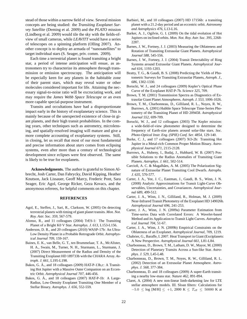
stead of those within a narrow field of view. Several missionconcepts are being studied: theTransiting Exoplanet Sur-vey Satellite(Deming et al. 2009) and thePLATOmission(Lindberg et al. 2009) would tile the sky with the fields-of-view of small cameras, whileLEAVITTwould have a seriesof telescopes on a spinning platform (Olling 2007). An-other concept is to deploy an armada of “nanosatellites” totarget individual stars (S. Seager, priv. comm. 2009).

Each time a terrestrial planet is found transiting a brightstar, a period of intense anticipation will ensue, as as-tronomers try to characterize its atmosphere through trans-mission or emission spectroscopy. The anticipation willbe especially keen for any planets in the habitable zoneof their parent stars, which may reveal water or othermolecules considered important for life. Attaining the nec-essary signal-to-noise ratio will be excruciating work, andmay require theJames Webb Space Telescopeor an evenmore capable special-purpose instrument.

Transits and occultations have had a disproportionateimpact early in the history of exoplanetary science. This ismainly because of the unexpected existence of close-in gi-ant planets, and their high transit probabilities. In the com-ing years, other techniques such as astrometry, microlens-ing, and spatially-resolved imaging will mature and give amore complete accounting of exoplanetary systems. Still,in closing, let us recall that most of our most fundamentaland precise information aboutstarscomes from eclipsingsystems, even after more than a century of technologicaldevelopment since eclipses were first observed. The sameis likely to be true for exoplanets.

Acknowledgments. The author is grateful to Simon Al-brecht, Josh Carter, Dan Fabrycky, David Kipping, HeatherKnutson, Jack Lissauer, Geoff Marcy, Frederic Pont, SaraSeager, Eric Agol, George Ricker, Geza Kovacs, and theanonymous referees, for helpful comments on this chapter.

REFERENCES

Agol, E., Steffen, J., Sari, R., Clarkson, W. (2005) On detectingterrestrial planets with timing of giant planet transits.Mon. Not.Roy. Astr. Soc. 359, 567-579.

Alonso, R., and 11 colleagues (2004) TrES-1: The TransitingPlanet of a Bright K0 V Star.Astrophys. J. 613, L153-L156.

Anderson, D. R., and 20 colleagues (2010) WASP-17b: An Ultra-Low Density Planet in a Probable Retrograde Orbit.Astrophys-ical Journal 709, 159-167.

Baines, E. K., van Belle, G. T., ten Brummelaar, T. A., McAlister,H. A., Swain, M., Turner, N. H., Sturmann, L., Sturmann, J.(2007) Direct Measurement of the Radius and Density of theTransiting Exoplanet HD 189733b with the CHARA Array.As-troph. J. 661, L195-L198.

Bakos, G.A., and 18 colleagues (2009) HAT-P-13b,c: A Transit-ing Hot Jupiter with a Massive Outer Companion on an Eccen-tric Orbit. Astrophysical Journal 707, 446-456.

Bakos, G.A., and 18 colleagues (2007) HAT-P-1b: A Large-Radius, Low-Density Exoplanet Transiting One Member of aStellar Binary.Astrophys. J. 656, 552-559.

Barbieri, M., and 10 colleagues (2007) HD 17156b: a transitingplanet with a 21.2-day period and an eccentric orbit.Astronomyand Astrophysics 476, L13-L16.

Barker, A. J., Ogilvie, G. I. (2009) On the tidal evolution ofHotJupiters on inclined orbits.Mon. Not. Roy. Astr. Soc. 395, 2268-2287.

Barnes, J. W., Fortney, J. J. (2003) Measuring the Oblateness andRotation of Transiting Extrasolar Giant Planets.AstrophysicalJournal 588, 545-556.

Barnes, J. W., Fortney, J. J. (2004) Transit Detectability of RingSystems around Extrasolar Giant Planets.Astrophysical Jour-nal 616, 1193-1203.

Beatty, T. G., & Gaudi, B. S. (2008) Predicting the Yields of Pho-tometric Surveys for Transiting Extrasolar Planets,Astroph. J.,686, 1302-1330.

Borucki, W. J., and 24 colleagues (2009) Kepler’s Optical PhaseCurve of the Exoplanet HAT-P-7b.Science 325, 709.

Brown, T. M. (2001) Transmission Spectra as Diagnostics of Ex-trasolar Giant Planet Atmospheres.Astroph. J. 553, 1006-1026.

Brown, T. M., Charbonneau, D., Gilliland, R. L., Noyes, R. W.,Burrows, A. (2001) Hubble Space Telescope Time-Series Pho-tometry of the Transiting Planet of HD 209458.AstrophysicalJournal 552, 699-709.

Borucki, W. J., and 12 colleagues (2003) The Kepler mission:a wide-field-of-view photometer designed to determine thefrequency of Earth-size planets around solar-like stars.Soc.Photo-Optical Instr. Eng. (SPIE) Conf. Ser. 4854, 129-140.

Burke, C. J., and 17 colleagues (2007) XO-2b: Transiting HotJupiter in a Metal-rich Common Proper Motion Binary.Astro-physical Journal 671, 2115-2128.

Burrows, A., Hubeny, I., Budaj, J., Hubbard, W. B. (2007) Pos-sible Solutions to the Radius Anomalies of Transiting GiantPlanets.Astrophys. J. 661, 502-514.

Carciofi, A. C. & Magalhaes, A. M. (2005) The Polarization Sig-nature of Extrasolar Planet Transiting Cool Dwarfs.Astrophs.J. 635, 570-577.

Carter, J. A., Yee, J. C., Eastman, J., Gaudi, B. S., Winn, J. N.(2008) Analytic Approximations for Transit Light-Curve Ob-servables, Uncertainties, and Covariances.Astrophysical Jour-nal 689, 499-512.

Carter, J. A., Winn, J. N., Gilliland, R., Holman, M. J. (2009)Near-Infrared Transit Photometry of the Exoplanet HD 149026b.Astrophysical Journal 696, 241-253.

Carter, J. A., Winn, J. N. (2009a) Parameter Estimation fromTime-series Data with Correlated Errors: A Wavelet-basedMethod and its Application to Transit Light Curves.Astrophys-ical Journal 704, 51-67.

Carter, J. A., Winn, J. N. (2009b) Empirical Constraints on theOblateness of an Exoplanet.Astrophysical Journal, 709, 1219.

Chabrier, G., Baraffe, I. 2007. Heat Transport in Giant (Exo)planets:A New Perspective.Astrophysical Journal 661, L81-L84.

Charbonneau, D., Brown, T. M., Latham, D. W., Mayor, M. (2000)Detection of Planetary Transits Across a Sun-like Star.Astro-phys. J. 529, L45-L48.

Charbonneau, D., Brown, T. M., Noyes, R. W., Gilliland, R. L.(2002) Detection of an Extrasolar Planet Atmosphere.Astro-phys. J. 568, 377-384.

Charbonneau, D. and 18 colleagues (2009) A super-Earth transit-ing a nearby low-mass star.Nature 462, 891-894.

Claret, A. (2004) A new non-linear limb-darkening law for LTEstellar atmosphere models. III. Sloan filters: Calculations for−5.0 ≤ log [M/H] ≤ +1, 2000 K≤ Teff ≤ 50000 K at

22

several surface gravities.Astron. Astroph. 428, 1001-1005.Claret, A. (2009) Does the HD 209458 planetary system pose a

challenge to the stellar atmosphere models?Astronomy andAstrophysics 506, 1335-1340.

Collier Cameron, A., and 31 colleagues (2007) Efficient identi-fication of exoplanetary transit candidates from SuperWASPlight curves.Monthly Notices of the Royal Astronomical Soci-ety 380, 1230-1244.

de Kort, J. J. M. A. (1954) Upper and lower limits for the ec-centricity and longitude of periastron of an eclipsing binary.Ricerche Astronomiche 3, 109-118.

Deming, D., and 11 colleagues (2009) Discovery and Character-ization of Transiting Super Earths Using an All-Sky TransitSurvey and Follow-up by the James Webb Space Telescope.Publications of the Astronomical Society of the Pacific 121,952-967.

Everett, M. E. & Howell, S. B. (2001) A Technique for Ultrahigh-Precision CCD Photometry.Publ. Astron. Soc. Pacific 113,1428-1435.

Fabrycky, D. C., Winn, J. N. (2009) Exoplanetary Spin-OrbitAlignment: Results from the Ensemble of Rossiter-McLaughlinObservations.Astroph. J. 696, 1230-1240.

Ford, E. B., Gaudi, B. S. (2006) Observational Constraints onTrojans of Transiting Extrasolar Planets.Astrophysical Jour-nal 652, L137-L140.

Fossey, S. J., Waldmann, I. P., Kipping, D. M. (2009) Detectionof a transit by the planetary companion of HD 80606.MonthlyNotices of the Royal Astronomical Society 396, L16-L20.

Garcia-Melendo, E., McCullough, P. R. (2009) Photometric De-tection of a Transit of HD 80606b.Astrophysical Journal 698,558-561.

Gaudi, B. S. (2005) On the Size Distribution of Close-in Extraso-lar Giant Planets.Astroph. J. 628, L73-L76

Gaudi, B. S., Seager, S., & Mallen-Ornelas, G. (2005) On the Pe-riod Distribution of Close-in Extrasolar Giant Planets.Astroph.J. 623, 472-481.

Gaudi, B. S., Winn, J. N. (2007) Prospects for the Characterizationand Confirmation of Transiting Exoplanets via the Rossiter-McLaughlin Effect.Astroph. J. 655, 550-563.

Gilliland, R. L., & Brown, T. M. (1988) Time-resolved CCD pho-tometry of an ensemble of stars.Publ. Astron. Soc. Pacific 100,754-765.

Gilliland, R. L., and 23 colleagues (2000) A Lack of Planets in 47Tucanae from a Hubble Space Telescope Search.Astrophys. J.545, L47-L51.

Gillon, M., Demory, B.-O., Barman, T., Bonfils, X., Mazeh, T.,Pont, F., Udry, S., Mayor, M., Queloz, D. (2007) AccurateSpitzer infrared radius measurement for the hot Neptune GJ436b.Astronomy and Astrophysics 471, L51-L54.

Gimenez, A. (2007) Equations for the analysis of the light curvesof extra-solar planetary transits.Astron. Astrophys. 474, 1049-1049.

Gregory, P. C. (2005)Bayesian Logical Data Analysis for thePhysical Sciences: A Comparative Approach with Mathemat-ica Support, Cambridge University Press

Grillmair, C. J., Burrows, A., Charbonneau, D., Armus, L., Stauf-fer, J., Meadows, V., van Cleve, J., von Braun, K., Levine, D.(2008) Strong water absorption in the dayside emission spec-trum of the planet HD189733b.Nature 456, 767-769.

Guillot, T., Santos, N. C., Pont, F., Iro, N., Melo, C., Ribas, I.(2006) A correlation between the heavy element content oftransiting extrasolar planets and the metallicity of theirparent

stars.Astron. Astroph. 453, L21-L24.Guillot, T., Showman, A. P. (2002) Evolution of “51 Pegasus b-

like” planets.Astronomy and Astrophysics 385, 156-165.Hebrard, G., and 22 colleagues (2008) Misaligned spin-orbit in the

XO-3 planetary system?Astron. Astrophys. 488, 763-770.Hellier, C., and 22 colleagues (2009) An orbital period of 0.94

days for the hot-Jupiter planet WASP-18b.Nature 460, 1098-1100.

Henry, G. W., Marcy, G. W., Butler, R. P., Vogt, S. S. (2000) ATransiting “51 Peg-like” Planet.Astrophys. J. 529, L41-L44

Hilditch, R. W. (2001)An Introduction to Close Binary Stars(Cambridge, UK: Cambridge University Press)

Holman, M. J., Murray, N. W. (2005) The Use of Transit Timing toDetect Terrestrial-Mass Extrasolar Planets.Science 307, 1288-1291.

Holman, M. J., Winn, J. N., Latham, D. W., O’Donovan, F. T.,Charbonneau, D., Bakos, G. A., Esquerdo, G. A., Hergen-rother, C., Everett, M. E., Pal, A. (2006) The Transit LightCurve Project. I. Four Consecutive Transits of the ExoplanetXO-1b.Astrophysical Journal 652, 1715-1723.

Horne, K. (2003) Status aand Prospects of Planetary TransitSearches: Hot Jupiters Galore. inScientific Frontiers in Re-search on Extrasolar Planets, ed. D. Deming and S. Seager,ASP Conference Series Vol. 294 (San Francisco: ASP), p.361-370.

Howell, S. B. (2006)Handbook of CCD astronomy(Cambridge,UK: Cambridge Univ. Press), 2nd ed.

Hubeny, I., Burrows, A., Sudarsky, D. (2003) A Possible Bifurca-tion in Atmospheres of Strongly Irradiated Stars and Planets.Astrophysical Journal 594, 1011-1018.

Jordan, A., Bakos, G.A. (2008) Observability of the General Rela-tivistic Precession of Periastra in Exoplanets.Astrophys. J. 685,543-552.

Kallrath, J. & Milone, E. F. (2009)Eclipsing Binary Stars: Mod-eling and Analysis(New York: Springer-New York), 2nd ed.,in press

Kane, S. R. (2007) Detectability of exoplanetary transits from ra-dial velocity surveys. Mon. Not. Roy. Astr. Soc. 380, 1488-1496.

Kipping, D. M. (2008) Transiting planets – light-curve analysisfor eccentric orbits.Mon. Not. Roy. Astr. Soc. 389, 1383-1390.

Kipping, D. M. (2009) Transit timing effects due to an exomoon.Mon. Not. Roy. Astr. Soc. 392, 181-189.

Kjeldsen, H. & Frandsen, S. (1992) High-precision time-resolvedCCD photometry.Publ. Astron. Soc. Pacific 104, 413-434.

Knutson, H. A., Charbonneau, D., Noyes, R. W., Brown, T. M.,Gilliland, R. L. (2007a) Using Stellar Limb-Darkening to Re-fine the Properties of HD 209458b.Astrophys. J. 655, 564-575.

Knutson, H. A., Charbonneau, D., Allen, L. E., Fortney, J. J.,Agol, E., Cowan, N. B., Showman, A. P., Cooper, C. S.,Megeath, S. T. (2007b) A map of the day-night contrast of theextrasolar planet HD 189733b.Nature 447, 183-186.

Kopal, Z. (1979) Language of the stars: A discourse on the theoryof the light changes of eclipsing variables.Astrophysics andSpace Science Library 77, Kluwer, Dordrecht.

Kovacs, G., Zucker, S., Mazeh, T. (2002) A box-fitting algorithmin the search for periodic transits.Astronomy and Astrophysics391, 369-377.

Kovacs, G., Bakos, G., Noyes, R. W. 2005. A trend filtering algo-rithm for wide-field variability surveys.Monthly Notices of theRoyal Astronomical Society 356, 557-567.

Laughlin, G., Deming, D., Langton, J., Kasen, D., Vogt, S., But-

23

ler, P., Rivera, E., Meschiari, S. (2009) Rapid heating of theatmosphere of an extrasolar planet.Nature 457, 562-564.

Leger, A., and 160 colleagues (2009) Transiting exoplanets fromthe CoRoT space mission. VIII. CoRoT-7b: the first super-Earth with measured radius.Astronomy and Astrophysics 506,287-302.

Lindberg, R., Stankov, A., Fridlund, M., Rando, N. (2009) Currentstatus of the assessment of the ESA Cosmic Vision missioncandidate PLATO.Proceedings of the SPIE 7440, 7440Z-1 to7440Z-12

Madhusudhan, N., Seager, S. (2009) A Temperature and Abun-dance Retrieval Method for Exoplanet Atmospheres.Astro-physical Journal 707, 24-39.

Madhusudhan, N., Winn, J. N. (2009) Empirical Constraints onTrojan Companions and Orbital Eccentricities in 25 TransitingExoplanetary Systems.Astrophysical Journal 693, 784-793.

Mandel, K., Agol, E. (2002) Analytic Light Curves for PlanetaryTransit Searches.Astrophys. J. 580, L171-L175.

Marzari, F., Nelson, A. F. (2009) Interaction of a Giant Planet in anInclined Orbit with a Circumstellar Disk.Astrophysical Jour-nal 705, 1575-1583.

Mazeh, T., and 19 colleagues (2000) The Spectroscopic Orbitofthe Planetary Companion Transiting HD 209458.Astrophysi-cal Journal 532, L55-L58.

Mazeh, T., Zucker, S., Pont, F. (2005) An intriguing correlationbetween the masses and periods of the transiting planets.Mon.Not. Roy. Astr. Soc. 356, 955-957.

McCullough, P. R., Stys, J. E., Valenti, J. A., Fleming, S. W.,Janes, K. A., Heasley, J. N. (2005) The XO Project: Search-ing for Transiting Extrasolar Planet Candidates.Publ. Astron.Soc. Pacific 117, 783-795.

Miller, N., Fortney, J. J., Jackson, B. (2009) Inflating and DeflatingHot Jupiters: Coupled Tidal and Thermal Evolution of KnownTransiting Planets.Astrophysical Journal 702, 1413-1427.

Miralda-Escude, J. (2002) Orbital Perturbations of TransitingPlanets: A Possible Method to Measure Stellar Quadrupolesand to Detect Earth-Mass Planets.Astrophys. J. 564, 1019-1023.

Moutou, C., and 21 colleagues (2009) Photometric and spectro-scopic detection of the primary transit of the 111-day-periodplanet HD 80606b.Astronomy and Astrophysics 498, L5-L8.

Narita, N., Sato, B., Hirano, T., Tamura, M. (2009) First Evi-dence of a Retrograde Orbit of a Transiting Exoplanet HAT-P-7b. Publications of the Astronomical Society of Japan 61,L35-L40.

Nesvorny, D. (2009) Transit Timing Variations for Eccentric andInclined Exoplanets. Astrophysical Journal 701, 1116-1122.

Nutzman, P., Charbonneau, D. (2008) Design Considerationsfor aGround-Based Transit Search for Habitable Planets Orbiting MDwarfs.Publications of the Astronomical Society of the Pacific120, 317-327.

O’Donovan, F. T., Charbonneau, D., Alonso, R., Brown, T. M.,Mandushev, G., Dunham, E. W., Latham, D. W., Stefanik,R. P., Torres, G., Everett, M. E. (2007) Outcome of Six Candi-date Transiting Planets from a TrES Field in Andromeda.As-trophys. J. 662, 658-668.

Olling, R. P. (2007) LEAVITT: A MIDEX-class Mission for Find-ing and Characterizing 10,000 Transiting Planets in the SolarNeighborhood. ArXiv e-prints arXiv:0704.3072.

Pal, A., Kocsis, B. (2008) Periastron precession measurements intransiting extrasolar planetary systems at the level of generalrelativity. Monthly Notices of the Royal Astronomical Society

389, 191-198.Pepper, J., Gould, A., Depoy, D. L. (2003) Using All-Sky Surveys

to Find Planetary Transits.Acta Astronomica 53, 213-228.Pollacco, D. L., and 27 colleagues (2006) The WASP Project

and the SuperWASP Cameras.Publ. Astron. Soc. Pacific 118,1407-1418.

Pont, F., Zucker, S., Queloz, D. (2006) The effect of red noiseon planetary transit detection.Monthly Notices of the RoyalAstronomical Society 373, 231-242.

Pont, F., Knutson, H., Gilliland, R. L., Moutou, C., Charbon-neau, D. (2008) Detection of atmospheric haze on an extra-solar planet: the 0.55-1.05µm transmission spectrum of HD189733b with the Hubble Space Telescope.Mon. Not. Roy.Astr. Soc. 385, 109-118.

Press, W. H., Teukolsky, S. A., Vetterling, W. T., & Flannery, B. P.(2007) Numerical Recipes: The Art of Scientific Computing,3rd ed., Cambridge University Press

Queloz, D., and 39 colleagues (2009) The CoRoT-7 planetary sys-tem: two orbiting super-Earths.Astronomy and Astrophysics506, 303-319.

Rabus, M., Alonso, R., Belmonte, J. A., Deeg, H. J., Gilliland,R. L., Almenara, J. M., Brown, T. M., Charbonneau, D., Man-dushev, G. (2009) A cool starspot or a second transiting planetin the TrES-1 system?Astronomy and Astrophysics 494, 391-397.

Ragozzine, D., Wolf, A. S. (2009) Probing the Interiors of veryHot Jupiters Using Transit Light Curves.Astrophysical Journal698, 1778-1794.

Reiger, S. H. (1963) Starlight scintillation and atmospheric turbu-lence.Astronomical Journal 68, 395.

Rowe, J. F., and 10 colleagues (2008) The Very Low Albedo ofan Extrasolar Planet: MOST Space-based Photometry of HD209458.Astrophysical Journal 689, 1345-1353.

Russell, H. N. (1948) The royal road of eclipses.Harvard Coll.Obs. Monograph 7, 181-209.

Ryan, P., Sandler, D. (1998) Scintillation Reduction Method forPhotometric Measurements.Publications of the AstronomicalSociety of the Pacific 110, 1235-1248.

Sackett, P. (1999) Searching for Unseen Planets via Occultationand Microlensing, inPlanets Outside the Solar System: Theoryand Observations(J.-M. Mariotti and D. Alloin, eds.), p. 189,Kluwer, Dordrecht.

Sasselov, D. D. (2003) The New Transiting Planet OGLE-TR-56b:Orbit and Atmosphere.Astrophysical Journal 596, 1327-1331.

Sato, B., and 20 colleagues (2005) The N2K Consortium. II. ATransiting Hot Saturn around HD 149026 with a Large DenseCore.Astrophys. J. 633, 465-473.

Seager, S., Hui, L. (2002) Constraining the Rotation Rate ofTran-siting Extrasolar Planets by Oblateness Measurements.As-troph. J. 574, 1004-1010.

Seager, S., Mallen-Ornelas, G. (2003) A Unique Solution ofPlanetand Star Parameters from an Extrasolar Planet Transit LightCurve.Astroph. J. 585, 1038-1055.

Seager, S., Sasselov, D. D. (2000) Theoretical Transmission Spec-tra during Extrasolar Giant Planet Transits.Astroph. J. 537,916-921.

Sing, D. K., Desert, J.-M., Lecavelier Des Etangs, A., Ballester,G. E., Vidal-Madjar, A., Parmentier, V., Hebrard, G., Henry,G. W. (2009) Transit spectrophotometry of the exoplanetHD 189733b. I. Searching for water but finding haze withHST NICMOS.Astronomy and Astrophysics 505, 891-899.

Snellen, I. A. G., de Mooij, E. J. W., Albrecht, S. (2009) The

24

changing phases of extrasolar planet CoRoT-1b.Nature 459,543-545.

Southworth, J., Wheatley, P. J., Sams, G. (2007) A method forthe direct determination of the surface gravities of transitingextrasolar planets.Mon. Not. Roy. Astr. Soc. 379, L11-L15.

Southworth, J. (2008) Homogeneous studies of transiting extraso-lar planets. I. Light-curve analyses.Mon. Not. Roy. Astr. Soc.386, 1644-1666.

Southworth, J. (2009) Homogeneous studies of transiting extra-solar planets - II. Physical properties.Monthly Notices of theRoyal Astronomical Society 394, 272-294.

Stello, D., and 24 colleagues (2009) Radius Determination ofSolar-type Stars Using Asteroseismology: What to Expectfrom the Kepler Mission.Astroph. J. 700, 1589-1602.

Sterne, T. E. 1940. On the Determination of the Orbital Elementsof Eccentric Eclipsing Binaries.Proc. Nat. Ac. Sci. 26, 36-40.

Struve, O. (1952) Proposal for a project of high-precision stellarradial velocity work.The Observatory 72, 199-200.

Swain, M. R., Vasisht, G., Tinetti, G. (2008) The presence ofmethane in the atmosphere of an extrasolar planet.Nature 452,329-331.

Swain, M. R., Vasisht, G., Tinetti, G., Bouwman, J., Chen, P.,Yung, Y., Deming, D., Deroo, P. (2009) Molecular Signaturesin the Near-Infrared Dayside Spectrum of HD 189733b.Astro-phys. J. 690, L114-L117.

Tamuz, O., Mazeh, T., Zucker, S. (2005) Correcting systematic ef-fects in a large set of photometric light curves.Monthly Noticesof the Royal Astronomical Society 356, 1466-1470.

Tinetti, G., and 12 colleagues (2007) Water vapour in the atmo-sphere of a transiting extrasolar planet.Nature 448, 169-171.

Torres, G., Winn, J. N., Holman, M. J. (2008) Improved Parame-ters for Extrasolar Transiting Planets.Astrophys. J. 677, 1324-1342.

Torres, G., and 15 colleagues (2007) HAT-P-3b: A Heavy-Element-rich Planet Transiting a K Dwarf Star.Astrophys. J.666, L121-L124.

Udalski, A., Paczynski, B., Zebrun, K., Szymanski, M., Kubiak,M., Soszynski, I., Szewczyk, O., Wyrzykowski, L., Pietrzyn-ski, G. (2002) The Optical Gravitational Lensing Experiment.Search for Planetary and Low-Luminosity Object Transits inthe Galactic Disk. Results of 2001 Campaign.Acta Astronom-ica 52, 1-37.

Vidal-Madjar, A., Lecavelier des Etangs, A., Desert, J.-M.,Ballester, G. E., Ferlet, R., Hebrard, G., Mayor, M. (2003)An extended upper atmosphere around the extrasolar planetHD209458b.Nature 422, 143-146.

Weldrake, D. T. F., Sackett, P. D., Bridges, T. J., Freeman, K. C.(2005) An Absence of Hot Jupiter Planets in 47 Tucanae: Re-sults of a Wide-Field Transit Search.Astroph. J. 620, 1043-1051.

Winn, J. N., Holman, M. J., Roussanova, A. (2007a) The TransitLight Curve Project. III. Tres Transits of TrES-1.AstrophysicalJournal 657, 1098-1106.

Winn, J. N., and 10 colleagues (2007b) The Transit Light CurveProject. V. System Parameters and Stellar Rotation Period ofHD 189733.Astronomical Journal 133, 1828-1835.

Winn, J. N., Henry, G. W., Torres, G., Holman, M. J. (2008) FiveNew Transits of the Super-Neptune HD 149026b.Astrophysi-cal Journal 675, 1531-1537.

Winn, J. N., and 10 colleagues (2009a) On the Spin-Orbit Mis-alignment of the XO-3 Exoplanetary System.AstrophysicalJournal 700, 302-308.

Winn, J. N., Johnson, J. A., Albrecht, S., Howard, A. W., Marcy,G. W., Crossfield, I. J., Holman, M. J. (2009b) HAT-P-7: ARetrograde or Polar Orbit, and a Third Body.AstrophysicalJournal 703, L99-L103.

Young, A. T. (1967) Photometric error analysis. VI. Confirmationof Reiger’s theory of scintillation.Astronomical Journal 72,747.

Zahnle, K., Marley, M. S., Freedman, R. S., Lodders, K., Fort-ney, J. J. (2009) Atmospheric Sulfur Photochemistry on HotJupiters.Astrophysical Journal 701, L20-L24.

25