The Cryosphere, 6, 1157–1162, 2012www.the-cryosphere.net/6/1157/2012/doi:10.5194/tc-6-1157-2012© Author(s) 2012. CC Attribution 3.0 License.

The Cryosphere

Transition in the fractal geometry of Arctic melt ponds

C. Hohenegger1, B. Alali1, K. R. Steffen1, D. K. Perovich2,3, and K. M. Golden1

1Department of Mathematics, University of Utah, 155 S 1400 E, RM 233, Salt Lake City, UT 84112–0090, USA2ERDC-CRREL, 72 Lyme Road, Hanover, NH 03755, USA3Thayer School of Engineering, Dartmouth College, Hanover, NH 03755, USA

Correspondence to:K. M. Golden (golden@math.utah.edu)

Received: 4 May 2012 – Published in The Cryosphere Discuss.: 15 June 2012Revised: 19 September 2012 – Accepted: 20 September 2012 – Published: 19 October 2012

Abstract. During the Arctic melt season, the sea ice surfaceundergoes a remarkable transformation from vast expansesof snow covered ice to complex mosaics of ice and meltponds. Sea ice albedo, a key parameter in climate model-ing, is determined by the complex evolution of melt pondconfigurations. In fact, ice–albedo feedback has played amajor role in the recent declines of the summer Arctic seaice pack. However, understanding melt pond evolution re-mains a significant challenge to improving climate projec-tions. By analyzing area–perimeter data from hundreds ofthousands of melt ponds, we find here an unexpected sep-aration of scales, where pond fractal dimensionD transitionsfrom 1 to 2 around a critical length scale of 100 m2 in area.Pond complexity increases rapidly through the transition assmaller ponds coalesce to form large connected regions, andreaches a maximum for ponds larger than 1000 m2, whoseboundaries resemble space-filling curves, withD ≈ 2. Theseuniversal features of Arctic melt pond evolution are similarto phase transitions in statistical physics. The results impactsea ice albedo, the transmitted radiation fields under melt-ing sea ice, the heat balance of sea ice and the upper ocean,and biological productivity such as under ice phytoplanktonblooms.

1 Introduction

Melt ponds on the surface of sea ice form a key compo-nent of the late spring and summer Arctic marine environ-ment (Flocco et al., 2010; Scott and Feltham, 2010; Pedersenet al., 2009; Polashenski et al., 2012). While snow and sea icereflect most incident sunlight, melt ponds absorb most of it.As melting increases so does solar absorption, which leads to

more melting, and so on. This ice–albedo feedback has con-tributed significantly to the precipitous losses of Arctic seaice (Perovich et al., 2008), which have outpaced the projec-tions of most climate models (Serreze et al., 2007; Stroeve etal., 2007; Boe et al., 2009). Representing the overall albedoof the sea ice pack is a fundamental problem in climate mod-eling (Flocco et al., 2010), and a significant source of uncer-tainty in efforts to improve climate projections.

Despite the central role that melt ponds play in understand-ing the decline of the summer Arctic sea ice pack, compre-hensive observations or theories of their formation, cover-age, and evolution remain relatively sparse. Available obser-vations of melt ponds show that their areal coverage is highlyvariable, particularly for first-year ice early in the melt sea-son, with rates of change as high as 35 % per day (Scharienand Yackel, 2005; Polashenski et al., 2012). Such variability,as well as the influence of many competing factors control-ling melt pond evolution (Eicken et al., 2002, 2004), makesthe incorporation of realistic treatments of albedo into seaice and climate models quite challenging (Polashenski etal., 2012). There have been substantial efforts at develop-ing detailed small- and medium-scale numerical models ofmelt pond coverage which include some of these mecha-nisms (Flocco and Feltham, 2007; Skyllingstad et al., 2009;Scott and Feltham, 2010). There has also been recent workon incorporating melt pond parameterizations into global cli-mate models (Flocco et al., 2010; Hunke and Lipscomb,2010; Pedersen et al., 2009).

Here we ask if the evolution of melt pond geometry ex-hibits universal characteristics which do not depend on thedetails of the driving mechanisms. Fundamentally, the melt-ing of Arctic sea ice during summer is a phase transitionphenomenon, where solid ice turns to liquid, albeit on large

Published by Copernicus Publications on behalf of the European Geosciences Union.

1158 C. Hohenegger et al.: Transition in the fractal geometry of Arctic melt ponds

regional scales and over a period of time which depends onenvironmental forcing and other factors. As such, we lookfor features of this important process which are mathemati-cally analogous to related phenomena in the theory of phasetransitions (Thompson, 1988; Coniglio, 1989). For example,the behavior displayed by the percolation model for con-nectedness of the phases in binary composites is similar tomelt pond evolution (Stauffer and Aharony, 1992; Torquato,2002; Christensen and Moloney, 2005). In both cases thereis a transition in the global geometrical characteristics of theconfigurations when the driving parameter exceeds a criticalthreshold.

2 Method

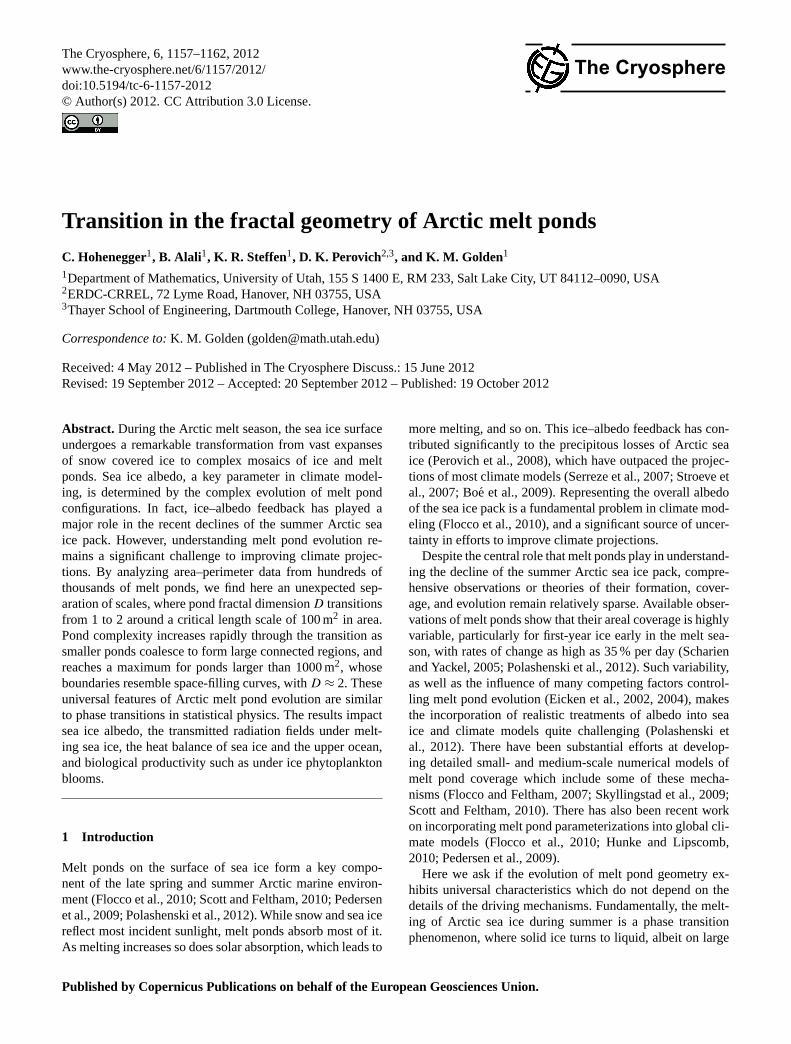
The sea ice surface is viewed here as a two phase compos-ite (Milton, 2002; Torquato, 2002) of dark melt ponds andwhite snow or ice (Fig.1). We investigate the geometry ofthe multiscale boundary between the two phases and how itevolves, as well as the connectedness of the melt pond phase.

We use two large sets of images of melting Arctic seaice collected during two Arctic expeditions: 2005Healy–OdenTRans Arctic EXpedition (HOTRAX) (Perovich et al.,2009) and 1998 Surface Heat Budget of the Arctic Ocean(SHEBA) (Perovich et al., 2002). The sea ice around SHEBAin the summer of 1998 was predominantly multiyear, withcoverage greater than 90 % (Perovich et al., 2002). Therewere a few scattered areas of first-year ice, where leads hadopened and frozen during the winter of 1997–1998. The HO-TRAX images from 14 August were of a transition zone be-tween first-year and multiyear ice. Ship-based ice observa-tions made on 14 August indicated a 5 to 3 ratio of multiyearto first-year ice (Perovich et al., 2009).

During the HOTRAX campaign, ten helicopter photo-graphic survey flights following a modified rectangular pat-tern around theHealy were conducted during the transitionfrom Arctic summer to fall (August–September) at an alti-tude between 500 m and 2000 m. Images were recorded witha Nikon D70 mounted on the helicopter with the interval-ometer set to ten seconds, resulting in almost no photo over-laps. During the SHEBA campaign, about a dozen helicoptersurvey flights following a box centered on theDes Groseil-liers were conducted between May and October, typically atan altitude of 1830 m. Images were recorded with a Nikon35 mm camera mounted on the back of the helicopter. Againminimal overlap between pictures was seen.

Recorded images show three distinct and geometricallycomplex features: open ocean, melt ponds and ice. The HO-TRAX images are easier to analyze, as the histograms ofthe RGB pixel values are clearly bimodal. In this case, iceis characterized by high red pixel values, while water cor-responds to lower red pixel values. Moreover, the transitionbetween shallow to deep water follows the blue spectrumfrom light to dark with ocean being almost black (Fig.2a).

Discussion

Pa

per|

Discussion

Paper

|D

iscussionP

aper

|D

iscussionP

aper

|

Fig. 1. Complex geometry of well developed Arctic melt ponds. Aerial photo taken 14 August2005 on the Healy-Oden Trans Arctic Expedition (HOTRAX).

14

Fig. 1. Complex geometry of well developed Arctic melt ponds.Aerial photo taken 14 August 2005 on theHealy–OdenTrans ArcticExpedition (HOTRAX).

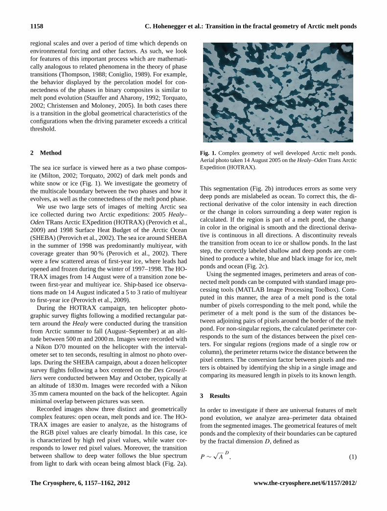
This segmentation (Fig.2b) introduces errors as some verydeep ponds are mislabeled as ocean. To correct this, the di-rectional derivative of the color intensity in each directionor the change in colors surrounding a deep water region iscalculated. If the region is part of a melt pond, the changein color in the original is smooth and the directional deriva-tive is continuous in all directions. A discontinuity revealsthe transition from ocean to ice or shallow ponds. In the laststep, the correctly labeled shallow and deep ponds are com-bined to produce a white, blue and black image for ice, meltponds and ocean (Fig.2c).

Using the segmented images, perimeters and areas of con-nected melt ponds can be computed with standard image pro-cessing tools (MATLAB Image Processing Toolbox). Com-puted in this manner, the area of a melt pond is the totalnumber of pixels corresponding to the melt pond, while theperimeter of a melt pond is the sum of the distances be-tween adjoining pairs of pixels around the border of the meltpond. For non-singular regions, the calculated perimeter cor-responds to the sum of the distances between the pixel cen-ters. For singular regions (regions made of a single row orcolumn), the perimeter returns twice the distance between thepixel centers. The conversion factor between pixels and me-ters is obtained by identifying the ship in a single image andcomparing its measured length in pixels to its known length.

3 Results

In order to investigate if there are universal features of meltpond evolution, we analyze area–perimeter data obtainedfrom the segmented images. The geometrical features of meltponds and the complexity of their boundaries can be capturedby the fractal dimensionD, defined as

P ∼√

AD

, (1)

The Cryosphere, 6, 1157–1162, 2012 www.the-cryosphere.net/6/1157/2012/

C. Hohenegger et al.: Transition in the fractal geometry of Arctic melt ponds 1159

Discussion

Paper

|D

iscussionP

aper|

Discussion

Paper

|D

iscussionP

aper|

a b c

Fig. 2. Image segmentation for 14 August (HOTRAX). Starting with the original image in (a),the image is initially segmented in (b) using a four color threshold with ice, shallow ponds, deepponds and ocean/deep ponds colored as white, green, red and black, respectively. In the laststep, deep and shallow ponds are differentiated from ocean and recombined in the final white,blue and black image (c) for ice, melt ponds and ocean.

15

Fig. 2. Image segmentation for 14 August (HOTRAX). Starting with the original image in(a), the image is initially segmented in(b) usinga four color threshold with ice, shallow ponds, deep ponds and ocean/deep ponds colored as white, green, red and black, respectively. In thelast step, deep and shallow ponds are differentiated from ocean and recombined in the final white, blue and black image(c) for ice, meltponds and ocean, respectively.

whereA andP are the area and perimeter, respectively. Onlogarithmic scales the slope characterizing theA–P data isone-half the fractal dimension. For regular objects like cir-cles and polygons, the perimeter scales like the square rootof the area, andD = 1. For objects with more highly ramifiedstructure, such as a Koch snowflake,D > 1. As the boundarybecomes increasingly complex and starts filling two dimen-sional space,P ∼ A and thenD ≈ 2. We remark thatD = 2is the upper bound for the two dimensional fractal exponent,and corresponds to space-filling curves (Sagan, 1994).

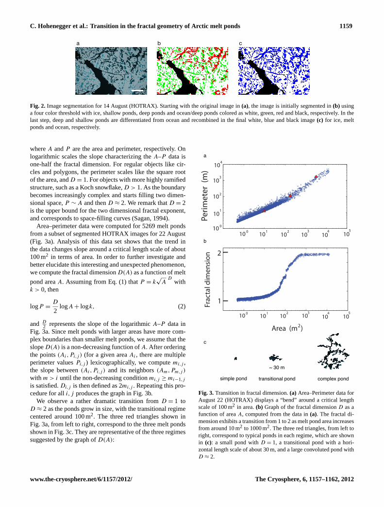
Area–perimeter data were computed for 5269 melt pondsfrom a subset of segmented HOTRAX images for 22 August(Fig. 3a). Analysis of this data set shows that the trend inthe data changes slope around a critical length scale of about100 m2 in terms of area. In order to further investigate andbetter elucidate this interesting and unexpected phenomenon,we compute the fractal dimensionD(A) as a function of melt

pond areaA. Assuming from Eq. (1) thatP = k√

AD

withk > 0, then

logP =D

2logA + logk, (2)

and D2 represents the slope of the logarithmicA–P data in

Fig. 3a. Since melt ponds with larger areas have more com-plex boundaries than smaller melt ponds, we assume that theslopeD(A) is a non-decreasing function ofA. After orderingthe points(Ai,Pi,j ) (for a given areaAi , there are multipleperimeter valuesPi,j ) lexicographically, we computemi,j ,the slope between(Ai,Pi,j ) and its neighbors(Am,Pm,j )

with m > i until the non-decreasing conditionmi,j ≥ mi−1,j

is satisfied.Di,j is then defined as 2mi,j . Repeating this pro-cedure for alli,j produces the graph in Fig.3b.

We observe a rather dramatic transition fromD = 1 toD ≈ 2 as the ponds grow in size, with the transitional regimecentered around 100 m2. The three red triangles shown inFig. 3a, from left to right, correspond to the three melt pondsshown in Fig.3c. They are representative of the three regimessuggested by the graph ofD(A):

Discussion

Paper

|D

iscussionP

aper|

Discussion

Paper

|D

iscussionP

aper|

Frac

tal d

imen

sion

10 0 1 2 3 41010 10 105

10

Area (m )2

2

1

10 0 1 2 3 41010 10

10

1

2

3

4

10

10

10

105

1010 0

Perim

eter

(m

)

complex pond

~ 30 m

simple pond transitional pond

(a)

(b)

(c)

a

b

simple pond

c

transitional pond complex pond

~ 30 m

Fig. 3. Transition in fractal dimension. (a) Area-Perimeter data for August 22 (HOTRAX) dis-plays a “bend” around a critical length scale of 100 m2 in area. (b) Graph of the fractal dimensionD as a function of area A, computed from the data in (a). The fractal dimension exhibits a tran-sition from 1 to 2 as melt pond area increases from around 10 m2 to 1000 m2. The three redtriangles, from left to right, correspond to typical ponds in each regime, which are shown in (c):a small pond with D = 1, a transitional pond with a horizontal length scale of about 30 m, and alarge convoluted pond with D ≈ 2.

16

Fig. 3. Transition in fractal dimension.(a) Area–Perimeter data forAugust 22 (HOTRAX) displays a “bend” around a critical lengthscale of 100 m2 in area.(b) Graph of the fractal dimensionD as afunction of areaA, computed from the data in(a). The fractal di-mension exhibits a transition from 1 to 2 as melt pond area increasesfrom around 10 m2 to 1000 m2. The three red triangles, from left toright, correspond to typical ponds in each regime, which are shownin (c): a small pond withD = 1, a transitional pond with a hori-zontal length scale of about 30 m, and a large convoluted pond withD ≈ 2.

www.the-cryosphere.net/6/1157/2012/ The Cryosphere, 6, 1157–1162, 2012

1160 C. Hohenegger et al.: Transition in the fractal geometry of Arctic melt ponds

1. A < 10 m2: simple ponds with Euclidean boundariesandD ≈ 1.

2. 10 m2 < A < 1000 m2: transitional ponds where com-plexity increases rapidly with size.

3. A > 1000 m2: self-similar ponds where complexity issaturated andD ≈ 2.

The transitional length scale of about 100 m2, identifiedby the location of the “bend” in theA–P data, appears tobe about the same after analysis of hundreds of thousands ofmelt ponds from both SHEBA and HOTRAX.

4 Discussion

These results demonstrate that there is a separation of lengthscales in melt pond structure. Such findings can ultimatelylead to more realistic and efficient treatments of melt pondsand the melting process in climate models. For example, alarge connected pond which spans an ice floe is likely moreeffective at helping to break apart a floe than many smalldisconnected ponds. Moreover, a separation of scales in themicrostructure of a composite medium is a necessary con-dition for the implementation of numerous homogenizationschemes to calculate its effective properties. “Homogeniza-tion”, also known as “upscaling”, refers to a set of ideas andmethods in applied mathematics which address the problemof computing the effective behavior of inhomogeneous me-dia or systems. For example, consider an electrically insu-lating host containing uniformly dispersed conducting inclu-sions. Homogenization theory gives a range of mathemati-cal techniques for obtaining rigorous information about theeffective or overall conductivity of this composite (Milton,2002; Torquato, 2002). Thus, the existence of a scale sep-aration in the pond/ice composite implies that rigorous cal-culations of the effective albedo are amenable to powerfulhomogenization approaches. Similarly, techniques of mathe-matical homogenization can thus be applied to finding the ef-fective behavior of transmitted light through melt ponds andits influence on the heat balance of the upper ocean and bio-logical productivity. Our findings for the fractal dimension ofthe melt ponds and its variation are similar to results on thefractal dimensions of connected clusters in percolation andIsing models (Saleur and Duplantier, 1987; Coniglio, 1989).

Like melt ponds, clouds strongly influence Earth’s albedo.However, the geometric structure of clouds and rain areaswas found through similar calculations (Lovejoy, 1982) tohave a fractal dimension of 1.35. This result was constantover the entire range of accessible length scales, which is instark contrast to what we find here for Arctic melt ponds.Interestingly, sea ice floe size distributions display a similarseparation of scales with two fractal dimensions (Toyota etal., 2006).

To help understand the transitional behavior we observe inFig. 3, we consider the process of how small simple ponds

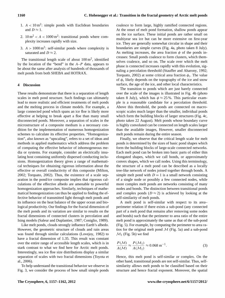
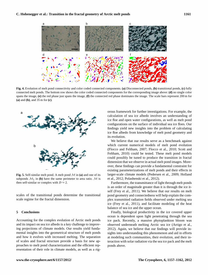
coalesce to form large, highly ramified connected regions.At the onset of melt pond formation, shallow ponds appearon the ice surface. These initial ponds are rather small onmultiyear sea ice but can be more extensive on first-yearice. They are generally somewhat circular in shape and theirboundaries are simple curves (Fig.4a, photo taken 8 July).As melting increases, the area fractionφ of the ponds in-creases: Small ponds coalesce to form clusters, which them-selves coalesce, and so on. The scale over which the meltphase is connected increases rapidly with this evolution, sig-naling a percolation threshold (Stauffer and Aharony, 1992;Torquato, 2002) at some critical area fractionφc. The valueof φc likely depends on the topography of the ice and snowsurface, the age of the ice, and other local characteristics.

The transition to ponds which are just barely connectedover the scale of the images is illustrated in Fig.4b (phototaken 8 July), which hasφ ≈ 25 %. This particular exam-ple is a reasonable candidate for a percolation threshold.Above this threshold, the ponds are connected on macro-scopic scales much larger than the smaller, individual pondswhich form the building blocks of larger structures (Fig.4c,photo taken 22 August). Melt ponds whose boundary curveis highly convoluted can be connected on length scales largerthan the available images, However, smaller disconnectedmelt ponds remain during the entire season.

Finally, we observe that the critical length scale for meltponds is determined by the sizes of basic pond shapes whichform the building blocks of large-scale connected networks.Each melt pond can be broken into basic parts of either thinelongated shapes, which we call bonds, or approximatelyconvex shapes, which we call nodes. Using this terminology,the structure of a melt pond can be described as a locallytree-like network of nodes joined together through bonds. Asimple melt pond withD = 1 is a small network consistingof a single node or possibly a few connected nodes, whilemore complex melt ponds are networks consisting of manynodes and bonds. The distinction between transitional pondsand complex ponds (D ≈ 2) is achieved by looking at theself-similarity of melt ponds.

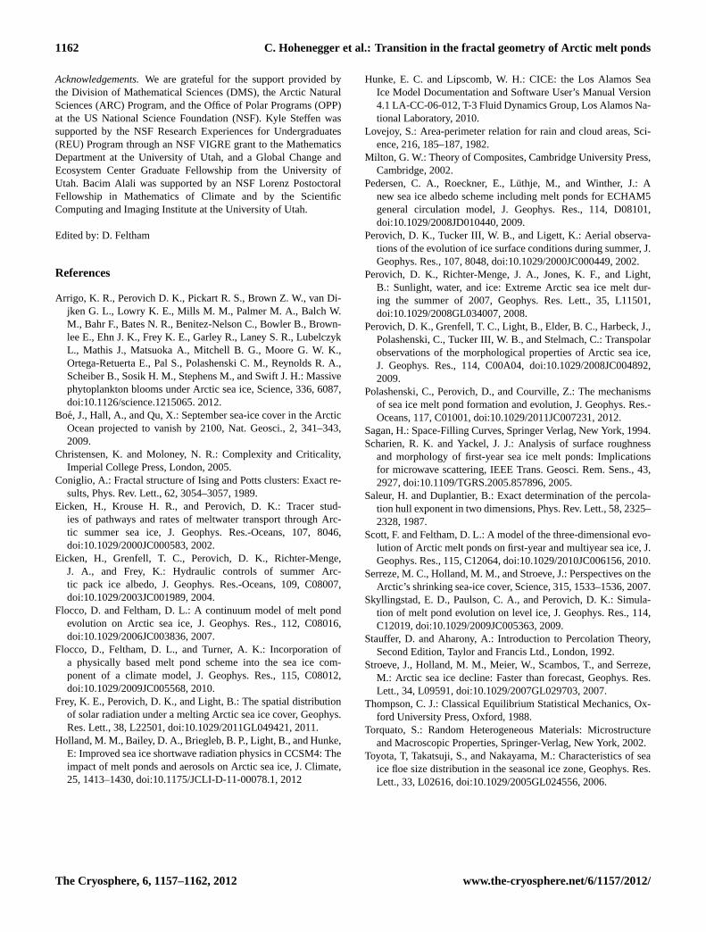
A melt pond is self-similar with respect to its area–perimeter relation if there exists a sub-pond (any connectedpart of a melt pond that remains after removing some nodesand bonds) such that the perimeter to area ratio of the entiremelt pond is approximately the same as that of the sub-pond(Fig. 5). For example, by computing the perimeter to area ra-tios for the original melt pondM (Fig. 5a) and a sub-pondM1 (Fig. 5b) we find

P(M)

A(M)≈

P(M1)

A(M1)≈ 0.068 m−1. (3)

Hence, this melt pond is self-similar or complex. On theother hand, transitional ponds are not self-similar. Thus, self-similarity allows melt ponds to be classified based on theirstructure and hence fractal exponent. Moreover, the spatial

The Cryosphere, 6, 1157–1162, 2012 www.the-cryosphere.net/6/1157/2012/

C. Hohenegger et al.: Transition in the fractal geometry of Arctic melt ponds 1161

Discussion

Paper

|D

iscussionP

aper|

Discussion

Paper

|D

iscussionP

aper|

a b c

fed

Fig. 4. Evolution of melt pond connectivity and color coded connected components. (a) Discon-nected ponds, (b) transitional ponds, (c) fully connected melt ponds. The bottom row showsthe color coded connected components for the corresponding image above: (d) no single colorspans the image, (e) the red phase just spans the image, (f) the connected red phase domi-nates the image. The scale bars represent 200 m for (a) and (b), and 35 m for (c).

17

Fig. 4.Evolution of melt pond connectivity and color coded connected components.(a) Disconnected ponds,(b) transitional ponds,(c) fullyconnected melt ponds. The bottom row shows the color coded connected components for the corresponding image above:(d) no single colorspans the image,(e) the red phase just spans the image,(f) the connected red phase dominates the image. The scale bars represent 200 m for(a) and(b), and 35 m for(c).

Discussion

Paper

|D

iscussionP

aper|

Discussion

Paper

|D

iscussionP

aper|

a

b

Fig. 5. Self-similar melt pond. A melt pond M and one of its sub-ponds M1 have the sameperimeter to area ratio. M is then self-similar or complex with D ≈ 2.

18

Fig. 5.Self-similar melt pond. A melt pondM in (a) and one of itssubpondsM1 in (b) have the same perimeter to area ratio.M isthen self-similar or complex withD ≈ 2.

scales of the transitional ponds determine the transitionalscale regime for the fractal dimension.

5 Conclusions

Accounting for the complex evolution of Arctic melt pondsand its impact on sea ice albedo is a key challenge to improv-ing projections of climate models. Our results yield funda-mental insights into the geometrical structure of melt pondsand how it evolves with increased melting. The separationof scales and fractal structure provide a basis for new ap-proaches to melt pond characterization and the efficient rep-resentation of their role in climate models, as well as a rig-

orous framework for further investigations. For example, thecalculation of sea ice albedo involves an understanding ofice floe and open water configurations, as well as melt pondconfigurations on the surface of individual sea ice floes. Ourfindings yield new insights into the problem of calculatingice floe albedo from knowledge of melt pond geometry andits evolution.

We believe that our results serve as a benchmark againstwhich current numerical models of melt pond evolution(Flocco and Feltham, 2007; Flocco et al., 2010; Scott andFeltham, 2010) could be tested. These melt pond modelscould possibly be tuned to produce the transition in fractaldimension that we observe in actual melt pond images. More-over, these findings can provide a fundamental constraint forexisting parameterizations of melt ponds and their effects inlarger-scale climate models (Pedersen et al., 2009; Hollandet al., 2012; Polashenski et al., 2012).

Furthermore, the transmittance of light through melt pondsis an order of magnitude greater than it is through the ice it-self (Frey et al., 2011). We believe that our results on meltpond geometry and connectedness will help explain the com-plex transmitted radiation fields observed under melting seaice (Frey et al., 2011), and facilitate modeling of the heatbalance of sea ice and the upper ocean.

Finally, biological productivity in the ice covered upperocean is dependent upon light penetrating through the seaice pack. Recently, a massive phytoplankton bloom wasobserved underneath melting Arctic sea ice (Arrigo et al.,2012). Again, we believe that our findings will provide in-sights into understanding this phenomenon and aid in effortsat modeling such communities, their evolution, and their in-teraction with solar radiation via the sea ice pack and the meltponds above.

www.the-cryosphere.net/6/1157/2012/ The Cryosphere, 6, 1157–1162, 2012

1162 C. Hohenegger et al.: Transition in the fractal geometry of Arctic melt ponds

Acknowledgements.We are grateful for the support provided bythe Division of Mathematical Sciences (DMS), the Arctic NaturalSciences (ARC) Program, and the Office of Polar Programs (OPP)at the US National Science Foundation (NSF). Kyle Steffen wassupported by the NSF Research Experiences for Undergraduates(REU) Program through an NSF VIGRE grant to the MathematicsDepartment at the University of Utah, and a Global Change andEcosystem Center Graduate Fellowship from the University ofUtah. Bacim Alali was supported by an NSF Lorenz PostoctoralFellowship in Mathematics of Climate and by the ScientificComputing and Imaging Institute at the University of Utah.

Edited by: D. Feltham

References

Arrigo, K. R., Perovich D. K., Pickart R. S., Brown Z. W., van Di-jken G. L., Lowry K. E., Mills M. M., Palmer M. A., Balch W.M., Bahr F., Bates N. R., Benitez-Nelson C., Bowler B., Brown-lee E., Ehn J. K., Frey K. E., Garley R., Laney S. R., LubelczykL., Mathis J., Matsuoka A., Mitchell B. G., Moore G. W. K.,Ortega-Retuerta E., Pal S., Polashenski C. M., Reynolds R. A.,Scheiber B., Sosik H. M., Stephens M., and Swift J. H.: Massivephytoplankton blooms under Arctic sea ice, Science, 336, 6087,doi:10.1126/science.1215065. 2012.

Boe, J., Hall, A., and Qu, X.: September sea-ice cover in the ArcticOcean projected to vanish by 2100, Nat. Geosci., 2, 341–343,2009.

Christensen, K. and Moloney, N. R.: Complexity and Criticality,Imperial College Press, London, 2005.

Coniglio, A.: Fractal structure of Ising and Potts clusters: Exact re-sults, Phys. Rev. Lett., 62, 3054–3057, 1989.

Eicken, H., Krouse H. R., and Perovich, D. K.: Tracer stud-ies of pathways and rates of meltwater transport through Arc-tic summer sea ice, J. Geophys. Res.-Oceans, 107, 8046,doi:10.1029/2000JC000583, 2002.

Eicken, H., Grenfell, T. C., Perovich, D. K., Richter-Menge,J. A., and Frey, K.: Hydraulic controls of summer Arc-tic pack ice albedo, J. Geophys. Res.-Oceans, 109, C08007,doi:10.1029/2003JC001989, 2004.

Flocco, D. and Feltham, D. L.: A continuum model of melt pondevolution on Arctic sea ice, J. Geophys. Res., 112, C08016,doi:10.1029/2006JC003836, 2007.

Flocco, D., Feltham, D. L., and Turner, A. K.: Incorporation ofa physically based melt pond scheme into the sea ice com-ponent of a climate model, J. Geophys. Res., 115, C08012,doi:10.1029/2009JC005568, 2010.

Frey, K. E., Perovich, D. K., and Light, B.: The spatial distributionof solar radiation under a melting Arctic sea ice cover, Geophys.Res. Lett., 38, L22501,doi:10.1029/2011GL049421, 2011.

Holland, M. M., Bailey, D. A., Briegleb, B. P., Light, B., and Hunke,E: Improved sea ice shortwave radiation physics in CCSM4: Theimpact of melt ponds and aerosols on Arctic sea ice, J. Climate,25, 1413–1430,doi:10.1175/JCLI-D-11-00078.1, 2012

Hunke, E. C. and Lipscomb, W. H.: CICE: the Los Alamos SeaIce Model Documentation and Software User’s Manual Version4.1 LA-CC-06-012, T-3 Fluid Dynamics Group, Los Alamos Na-tional Laboratory, 2010.

Lovejoy, S.: Area-perimeter relation for rain and cloud areas, Sci-ence, 216, 185–187, 1982.

Milton, G. W.: Theory of Composites, Cambridge University Press,Cambridge, 2002.

Pedersen, C. A., Roeckner, E., Luthje, M., and Winther, J.: Anew sea ice albedo scheme including melt ponds for ECHAM5general circulation model, J. Geophys. Res., 114, D08101,doi:10.1029/2008JD010440, 2009.

Perovich, D. K., Tucker III, W. B., and Ligett, K.: Aerial observa-tions of the evolution of ice surface conditions during summer, J.Geophys. Res., 107, 8048,doi:10.1029/2000JC000449, 2002.

Perovich, D. K., Richter-Menge, J. A., Jones, K. F., and Light,B.: Sunlight, water, and ice: Extreme Arctic sea ice melt dur-ing the summer of 2007, Geophys. Res. Lett., 35, L11501,doi:10.1029/2008GL034007, 2008.

Perovich, D. K., Grenfell, T. C., Light, B., Elder, B. C., Harbeck, J.,Polashenski, C., Tucker III, W. B., and Stelmach, C.: Transpolarobservations of the morphological properties of Arctic sea ice,J. Geophys. Res., 114, C00A04,doi:10.1029/2008JC004892,2009.

Polashenski, C., Perovich, D., and Courville, Z.: The mechanismsof sea ice melt pond formation and evolution, J. Geophys. Res.-Oceans, 117, C01001,doi:10.1029/2011JC007231, 2012.

Sagan, H.: Space-Filling Curves, Springer Verlag, New York, 1994.Scharien, R. K. and Yackel, J. J.: Analysis of surface roughness

and morphology of first-year sea ice melt ponds: Implicationsfor microwave scattering, IEEE Trans. Geosci. Rem. Sens., 43,2927,doi:10.1109/TGRS.2005.857896, 2005.

Saleur, H. and Duplantier, B.: Exact determination of the percola-tion hull exponent in two dimensions, Phys. Rev. Lett., 58, 2325–2328, 1987.

Scott, F. and Feltham, D. L.: A model of the three-dimensional evo-lution of Arctic melt ponds on first-year and multiyear sea ice, J.Geophys. Res., 115, C12064,doi:10.1029/2010JC006156, 2010.

Serreze, M. C., Holland, M. M., and Stroeve, J.: Perspectives on theArctic’s shrinking sea-ice cover, Science, 315, 1533–1536, 2007.

Skyllingstad, E. D., Paulson, C. A., and Perovich, D. K.: Simula-tion of melt pond evolution on level ice, J. Geophys. Res., 114,C12019,doi:10.1029/2009JC005363, 2009.

Stauffer, D. and Aharony, A.: Introduction to Percolation Theory,Second Edition, Taylor and Francis Ltd., London, 1992.

Stroeve, J., Holland, M. M., Meier, W., Scambos, T., and Serreze,M.: Arctic sea ice decline: Faster than forecast, Geophys. Res.Lett., 34, L09591,doi:10.1029/2007GL029703, 2007.

Thompson, C. J.: Classical Equilibrium Statistical Mechanics, Ox-ford University Press, Oxford, 1988.

Torquato, S.: Random Heterogeneous Materials: Microstructureand Macroscopic Properties, Springer-Verlag, New York, 2002.

Toyota, T, Takatsuji, S., and Nakayama, M.: Characteristics of seaice floe size distribution in the seasonal ice zone, Geophys. Res.Lett., 33, L02616,doi:10.1029/2005GL024556, 2006.

The Cryosphere, 6, 1157–1162, 2012 www.the-cryosphere.net/6/1157/2012/