K. Aatresh.MSc, Aerospace Department, IISc.

Prof B. N. Raghunandan.Aerospace Department, IISc.

Contents

Current Techniques

Literature review

Motivation & Objective

Formulation

Geometry & Simulation Results

Conclusions

Current Techniques Gauging

Book- Keeping Method

Gas Injection Method

Thermal Propellant Gauging Method

Acquisition

Use of Vanes and Sponges to maintain fuel

near the outlet

Literature Review Early work began after induction of the Apollo program in the

1960’s

Work by Petrash et al1 (1962) on estimation of propellant wetting times

Jaekle’s3 (1991) work on PMD design and

configuration

Studies on time response of cryogenic fuel by Fisher et.al4(1991)

Sasges et al’s5(1996) work on equilibrium states

Behavioral study on liquids in neutral buoyancy Venkatesh et al6(2001)

Study done on Marangoni bubble motion in zero gravity by Alhendal et.al8. The VOF module in ANSYS Fluent was used for simulation

Work by Lal & Raghunandan9 on the effect of surface tension on the fluid in microgravity condition

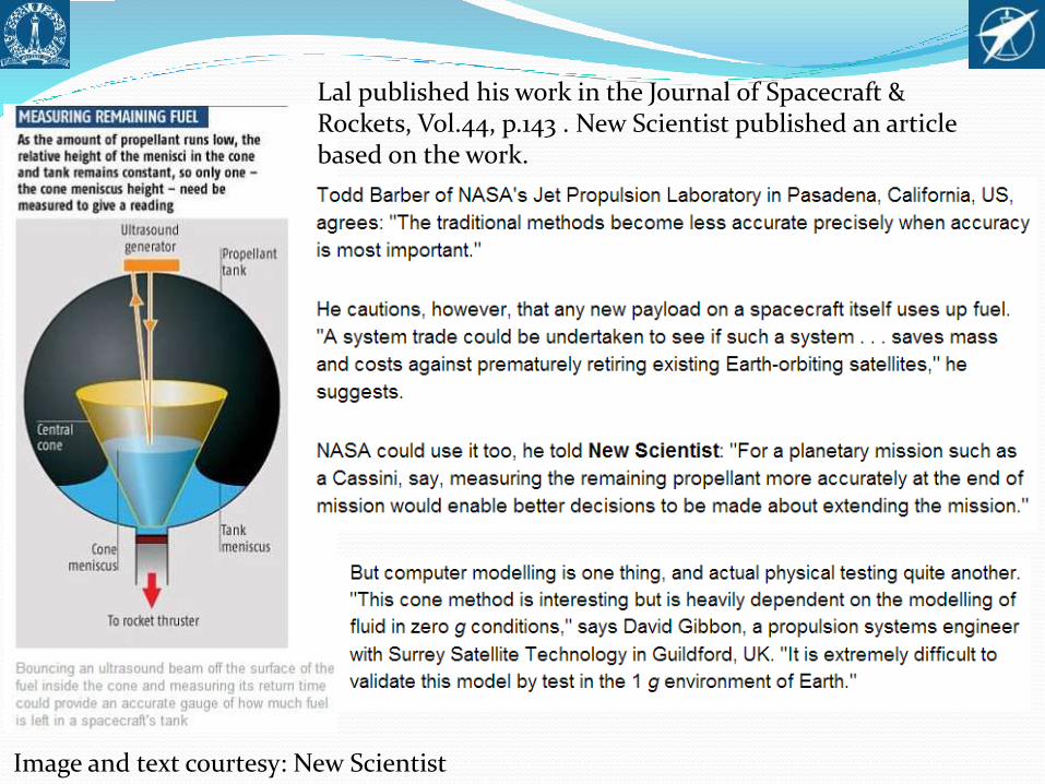
Image and text courtesy: New Scientist

Lal published his work in the Journal of Spacecraft & Rockets, Vol.44, p.143 . New Scientist published an article based on the work.

Motivation & Objectives Private letter addressed to Prof. Raghunandan from NASA Ames

Research Centre quoted as follows

“Is 4 minutes (or possibly up to 8, if absolutely required) long enough to test your fuel gauge approach? About how many flights would be required to truly advance development on this approach to fuel measurement?”

Whether technique can be experimentally tested another question raised by Surrey Satellite Technologies, UK.

Scales involved & duration for the state of microgravity to devise an experiment

Method to analyse motion of fluid in an enclosed container dominated by surface tension flows

Formulation ANSYS FLUENT v.13 chosen as the tool of choice to perform

computations

Volume of Fluid (VOF) Method chosen for the current problem

Alhendal et.al showed VOF method a robust numerical technique for the simulation of gas-liquid two phase flows and for simulation of surface tension flows

Air chosen as gaseous phase

Water and Hydrazine chosen as liquid phases.

First Order Upwind Scheme for spatial discretisation

Implicit Time Integration Scheme for temporal discretisation

SIMPLE algorithm used to calculate pressure field

Iterative time advancement scheme used to obtain solution till convergence

Residual tolerance for both the momentum and continuity equations was set to 10-4

Absolute values of residuals achieved found to be O(10−4) for velocities and O(10−4) for continuity

Validation Closed form solution comparison with

capillary rise of water in a 1 mm capillary

tube and a contact angle of 0o

Equilibrium height is 2.93 cm

Numerical simulation of

liquid rise in non-uniform

capillaries by Young

Transient capillary flows

by Robert

Young’s setup

Robert’s setup

Geometry & Simulation Results A 2D axisymmetric solver was used

The cone geometry used by Lal modified by adding cylindrical section

Quadrilateral paved mesh was chosen as the computational grid

Cone angle (α) varied to study change

of rise time

Grid independence examined through three levels of grid refinement with the 17o cone angle case with 26000, 33000 & 41000 cells

Difference reduced to less than 5% for rise height for fine and medium meshes

Liquid level kept horizontal in full scale(dia. = 2m) cases

Most of the liquid present in the annular space

Initial configuration of liquid. ( scale 1:1, cone angle 17o)

Comparison of rise heights for different mesh sizes.

Meniscus Height Simulations run for cone angles (α) of 17o, 21o and 28o

Equilibrium states taken from consecutive points with height difference of less than 1%

Results for the 17o degree cone angle case without and with cylindrical

section

Similar results obtained for rise rate for cone case of 21o

Liquid surface fluctuation without the cylindrical section

Found to be very slight (< 0.5% of the rise height)

Rise height similar in both cases with and & without cylindrical section

a) Initial state of liquid with flat surface. (b) Final equilibrium state.

(scale 1:1, cone angle 28o, with cylindrical section)

Rise rate of liquid surface in the cone with cylindrical section similar in characteristic to the previous cases

Addition of cylindrical section to the cone was found to increase the maximum rise height

Steeper and more steady rise rate as compared to cases without the cylindrical section

Has an effect similar to that of a sponge used in current PMDs

Cylindrical capillary seemed to aid the flow and the collection of fluid at the base

Scaling effects

Two scaled models of the 28o case simulated

1:0.5 and 1:0.1 scale

models of the original tank

(radius: 1m).

Simulation yields results

similar to full scale model

on different time scale as

expected.

Normalized height vs. time fordifferent scale models.(Cone angle 28o, with cylindricalsection)

Third simulation of the 1:0.1 scale model run with liquid spread in the tank

Configuration chosen to imitate general conditions found in propellant tank in microgravity

(a) Modified initial state of the liquid. (b) Final equilibrium state.

(scale 1:0.1, cone angle 28o.)

Simulations run with water & hydrazine for 1:0.1 scale without cylindrical section

Three different values of temperature; of 27oC, 50oC chosen.

Properties varied with temperature

Two values for contact angle of 0o and 5o chosen based on the work of Bernadin et.al8

Varying Surface Tension Values

Equilibrium times are far apart for water and hydrazine

Liquid meniscus found to be oscillating for the 5o contact angle case for hydrazine

Variation of rise heights not of much significance

Time scales obtained conducive for experimentation

Parameter(Constant)

Water Hydrazine

Equilibrium time (s)

Equilibrium height (m)

Equilibrium time (s)

Equilibrium height(m)

= 0o (T = 27oC)68

0.02 58.2 0.019

= 5o (T = 27oC) 50 0.017 64 0.02(max)

Temperature 10oC ( = 0o) 60 0.018 70 0.02

Temperature 50oC ( = 0o) 46 0.018 - -

changing physical conditions.(1:0.1 scale, initial liquid configuration: spread out state).

Variation with Gravity Study made with the change in gravitational level

Observed that as g kept reducing final equilibrium height increased.

Expected since a

reduction in the

gravitational force

magnifies the effects

of surface tension.

Effect of change in gravity on therising liquid meniscus. (1:0.1 scale, initial liquid configuration: spread out state).

Equilibrium State Time Scales Initial surface configuration taken flat, liquid volume fraction

10% and no liquid present in cone for full scale models

Cone angle (or)

Case

Type of Cone (or) Scale Equilibrium

Time (s)

Final

equilibrium

height (m)

17oWith cylindrical section (water) 960 0.74

Without cylindrical section (water) 530 0.63

21oWith cylindrical section (water) 940 0.55

Without cylindrical section (water) 780 0.58

28oWith cylindrical section (water) 900 0.72

Without cylindrical section (water) 940 0.36

Different scales of the 28o cone angle case

As scale is reduced clear order of magnitude reduction in equilibrium settling time is seen

Significant difference in settling times for 1:0.1 scale model with flat surface and 1:0.5 scale model

Type of Cone (or) Scale Initial Surface

Configuration

Equilibriu

m Time (s)

Final

equilibrium

height (m)

With cylindrical section, full

scale model Flat surface 900 0.72

With cylindrical section, half

scaled model Flat surface 68 0.22

With cylindrical section, 1/10th

scale model Flat surface 6.5 0.033

Conclusions Equilibrium times for all three cases were in order of 300 to 600

seconds for full scale models

Scaled down models of 1/10th scale have much lower values of settling time(of the order of tens of seconds)

Since the physics governing the propellant behaviour is the same irrespective of the scale, intermittent scale models between 1/10th and ½ with equilibrium times suitable to zero-g test

conditions can be used to study the geometry.

Formulation and the solution methodology are very general and hence applicable to any geometry of interest.

Scaled models can be used for experimental verification via parabolic flight path testing using fixed wing aircraft

References1. Donald A. Petrash, Robert F. Zappa, Edward W. Otto, “Technical Note –

Experimental Study of the Effects of Weightlessness on the Configuration of Mercury and Alcohol in Spherical Tanks”, Lewis Research Centre, 1962.

2. R. J. Hung. “Microgravity Liquid Propellant Management”, The University of Alabama in Huntsville Final Report, 1990.

3. D. E. Jaekle, Jr., “Propellant Management Device Conceptual Design and Analysis: Vanes”, AIAA-91-2172, 27th Joint Propulsion Conference, 1991.

4. M. F. Fisher, G. R. Schmidt, “Analysis of cryogenic propellant behaviour in microgravity and low thrust environments”, Cryogenics, Vol. 32, No. 2, pp. 230- 235, 1992.

5. M. R. Sasges, C. A. Ward, H. Azuma, S. Yoshihara, “Equilibrium fluid configurations in low gravity”, Journal of Applied Physics, 79(11), 1996.

6. H. S. Venkatesh, S. Krishnan, C. S. Prasad, K. L. Valiappan, G. Madhavan Nair, B. N. Raghunandan, “Behaviour of Liquids under Microgravity and Simulation using Neutral Buoyancy Model”, ESASP.454..221V, 2001.

7. Boris Yendler, Steven H. Collicott, Timothy A. Martin, “Thermal Gauging and Rebalancing of Propellant in Multiple Tank Satellites”, Journal of Spacecraft and Rockets, Vol.44, No. 4, 2007.

8. Yousuf Alhendal, Ali Turan, “Volume-of-Fluid (VOF) Simulations of Marangoni Bubble Motion in Zero Gravity”, Finite volume Method –Powerful Means of Engineering Design, pp. 215-234, 2012.

9. Amith Lal, B. N. Raghunandan, “Uncertainty Analysis of Propellant Gauging System for Spacecraft”, Journal of Spacecraft and Rockets, Vol.42, No.5, 2005.

Thank You