1

Hydraulic Pipe Transients by the Method of Characteristics By Gilberto E. Urroz, September 2004

NOTE: The formulations shown in this document are taken from Tullis, J.P., 1989 , Hydraulics of Pipelines – Pumps, Valves, Cavitation, Transients, John Wiley & Sons, New York Hydraulic Transients Hydraulic transients in pipelines occur when the steady-state conditions in a given point in the pipeline start changing with time, e.g., shutdown of a valve, failure of a pump, etc. In order to account for the disturbance in the steady-state conditions, a pressure wave will travel along the pipeline starting at the point of the disturbance and will be reflected back from the pipe boundaries (e.g., reservoirs) until a new steady-state is reached. The pressure waves in pipelines travel at a constant celerity as described next. Celerity of pressure waves in pipelines A pressure disturbance in a pipeline propagates with a very large wave celerity a given by

DEDKC

K

a

∆⋅⋅⋅

+=

1

ρ,

where K and ρ are the bulk modulus of elasticity and density of the fluid, D and ∆D are the inner diameter and the thickness of the pipe, E is the Young modulus (modulus of elasticity) of the pipe material, and C is a coefficient that accounts for the pipe support conditions:

• C = 1 – 0.5µ, if pipe is anchored at the upstream end only • C = 1-µ2, if pipe is anchored against any axial movement • C = 1, if each pipe section is anchored with expansion joints at each section

Here, µ represents the Poisson’s ratio of the material. For a perfectly rigid pipe, E is infinite, and the wave celerity simplifies to

ρKa = .

Equations of hydraulic transients The equations governing hydraulic transients are a pair of coupled, non-linear, first-order partial differential equations, namely,

2

02

||=

∂∂

+∂∂

++∂∂

tV

xVV

DVfV

xHg (momentum)

02

=∂∂

+∂

∂+

∂∂

xV

ga

tH

xHV , (continuity)

where H is the piezometric head (=z+p/g), V is the flow velocity, x is the distance along the pipe, t is time, g is the acceleration of gravity, f is the pipe friction factor (assumed constant), D is the pipe diameter, and a is the celerity of a pressure wave in the pipeline. These equations can be simplified by recognizing that the advective terms V∂V/∂x and V∂H/∂x, are negligible when compared to other terms in their corresponding equations. The resulting equations are, thus,

02

||=

∂∂

++∂∂

tV

DVfV

xHg (momentum)

02

=∂∂

+∂

∂xV

ga

tH (continuity)

The solution of the two transient equations require us to find the values of H(x,t) and V(x,t) in a domain defined by 0 < x < L, and 0 < t < tmax, where L is the length of the pipe, and tmax is an upper limit for the time domain. While the simultaneous solution of these two equations is possible through the use of finite differences, in this document we will approach the solution by determining the characteristic lines of the problem. Characteristics in pipe transients The characteristic lines for this case will be lines in the x-t plane defined by dx/dt = u(x,t), along which a function of H and V is conserved in time. Since the momentum and continuity equations shown above include partial derivatives of H and V with respect to x and t, we will try to reconstruct out of them expressions for the total derivatives of H and V, namely,

dH/dt = (∂H/∂x)(dx/dt)+ ∂H/∂t, and

dV/dt = (∂V/∂x)(dx/dt)+ ∂V/∂t. We start by adding the momentum equation to the continuity equation multiplied by a parameter λ, i.e.,

02

|| 2

=

∂∂

+∂

∂⋅+

∂∂

++∂∂

xV

ga

tH

tV

DVfV

xHg λ .

Expanding this equation and collecting terms that resemble the total derivatives dH/dt and dV/dt, produces:

3

02

||2

=+

∂∂

+∂∂

+

∂∂

+∂

∂⋅

DVfV

xV

ga

tV

xHg

tH λ

λλ (combined)

The terms between parentheses in this equation correspond to dH/dt and dV/dt, respectively, if we take dx/dt = g/λ for dH/dt and dx/dt = λa2/g for dV/dt. Since the two expressions for dx/dt must be the same, we have

λλ g

ga

=2

, or ag

±=λ .

Therefore, the characteristic lines are given by

adtdx

±= .

Since a is a constant value for pipelines, the characteristic lines are straight lines with slopes +a (referred to as a C+ line) and –a (referred to as a C- line). The combined equation listed above, after some manipulation, reduces to the two characteristic equations:

0||2

=±± VVgDaf

dtdV

ga

dtdH .

Most solutions are sought in terms of the pipeline discharge, Q = VA, rather than V, thus, the characteristic equations can be re-written as:

0||2 2 =++ QQ

gDAaf

dtdQ

gAa

dtdH , along C+: a

dtdx

+= ,

and

0||2 2 =−− QQ

gDAaf

dtdQ

gAa

dtdH , along C-: a

dtdx

−= .

Thus, the original systems of partial differential equations (momentum and continuity), has been reduced to the two characteristic equations (C+ and C-) along the corresponding characteristic lines, C+: dx/dt = +a, and C-: dx/dt = -a. Numerical solution grid A numerical solution of the transient problem in a pipeline will transport the values of H and Q along the characteristic lines as the time increases in increments ∆t. Calculation nodes can be placed along the pipeline separated by increments ∆x. The initial conditions of H and Q at t = 0, are then transported in time along the characteristic lines

4

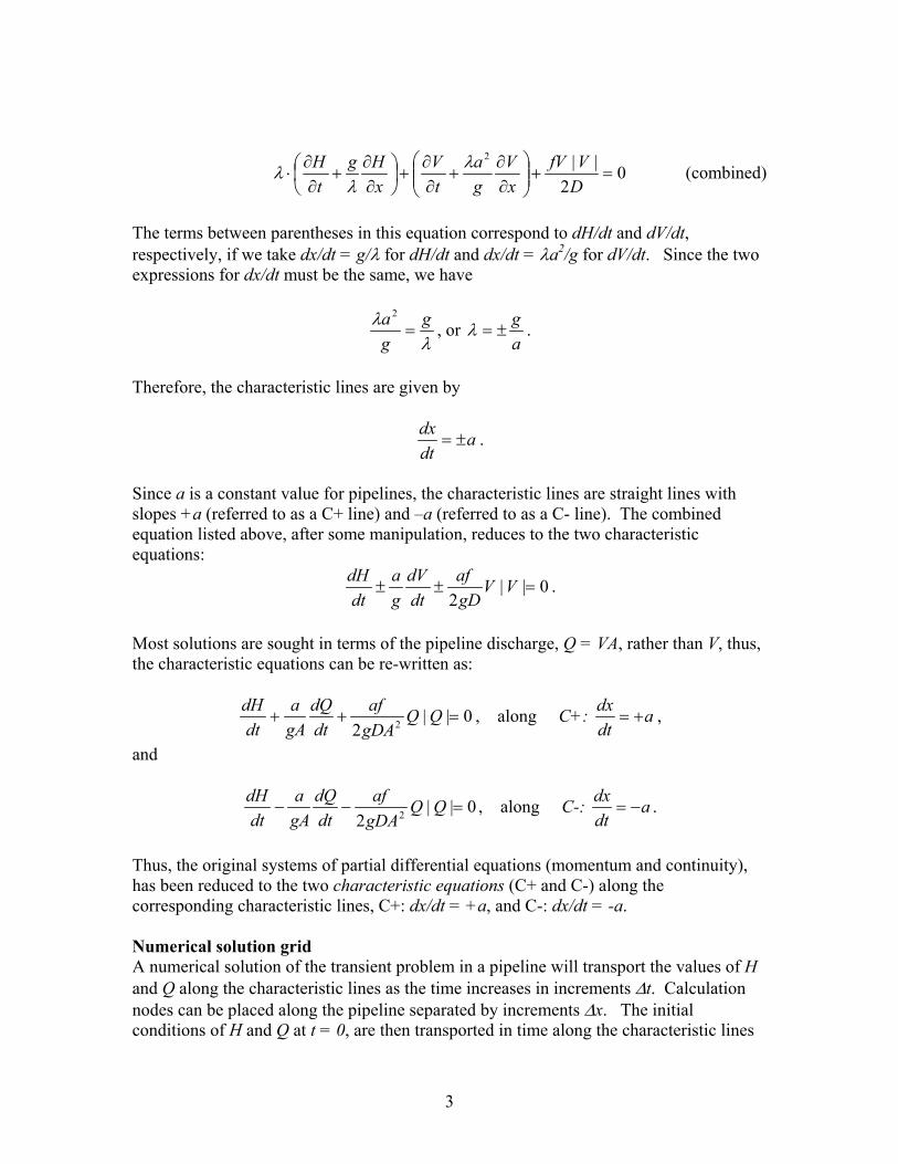
into the interior of the x-t solution domain. Boundary conditions at both extreme of the pipeline will be required to complete the solution. It is through these boundary conditions that a transient state is introduced into the system. Consider the case represented by the following figure. In its steady state, water flows from reservoir U (upstream) to reservoir D (downstream) through a horizontal pipeline of length L, diameter D, and Darcy-Weisbach friction factor f (assumed constant). The water levels in both reservoirs are given as HU and HD. A valve V at the entrance to reservoir D will be closed to produce the transient in the pipeline. For the time being we consider only friction losses in the pipe and localized losses through the valve.

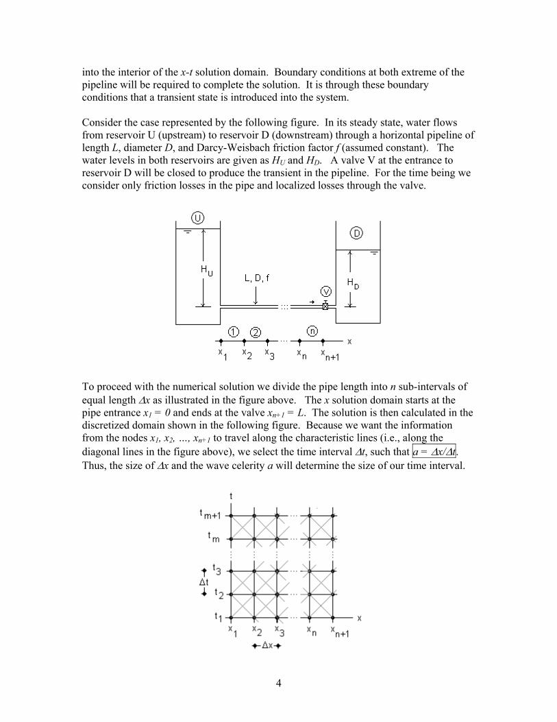
To proceed with the numerical solution we divide the pipe length into n sub-intervals of equal length ∆x as illustrated in the figure above. The x solution domain starts at the pipe entrance x1 = 0 and ends at the valve xn+1 = L. The solution is then calculated in the discretized domain shown in the following figure. Because we want the information from the nodes x1, x2, …, xn+1 to travel along the characteristic lines (i.e., along the diagonal lines in the figure above), we select the time interval ∆t, such that a = ∆x/∆t. Thus, the size of ∆x and the wave celerity a will determine the size of our time interval.

5

The numerical solution consists in determining the values of

Hij=H(xi,tj) and Qi

j=Q(xi,tj) at every grid point in the solution grid shown above. We selected n sub-intervals in x, such that ∆x = L/n, and m sub-intervals in time such that tmax = t1 + m∆t (typically, t1 = 0). The conditions at the starting time t1 = 0 (i.e., the initial conditions) are the steady state conditions before valve closure starts. Since the water level in reservoir U is constant, a boundary condition at x=x1 (the pipe entrance) is that H1

j=HU at any time level j. The boundary conditions at the valve V will be provided as a function of time. In other words, we will know how much the valve is being closed or the rate of closure and come up with a hydraulic equation to evaluate the head at the valve. Initial conditions The initial conditions are provided by the steady-state flow results. The energy equation written between the free-surfaces of the two reservoirs is

gV

DLf

gVKHH v

voDU 22

22

++= ,

where Kvo is the valve loss coefficient for steady state conditions (a function of the valve opening). With Vv = 4Qo/Av

2, and V = 4Qo/A2, where Av, A = valve and pipe cross-sectional areas, respectively, the solution for the steady-state discharge is

1

22

)(2i

v

v

DUo Q

DAfL

AK

HHgQ =+

−= .

Thus, the piezometric head at the upstream end is H1

1 = HU while that at the valve (upstream end) is

Hn+11 = HD+ 2

2

2 vv gA

QK .

The piezometric head at any distance x from the upstream end of the pipe can be calculated by using:

xgDAfQHxH U ⋅−= 2

2

2)( .

Therefore,

iUi xgDAfQHH ⋅−= 2

21

2, (H0)

for i = 1, 2, …, n+1.

6

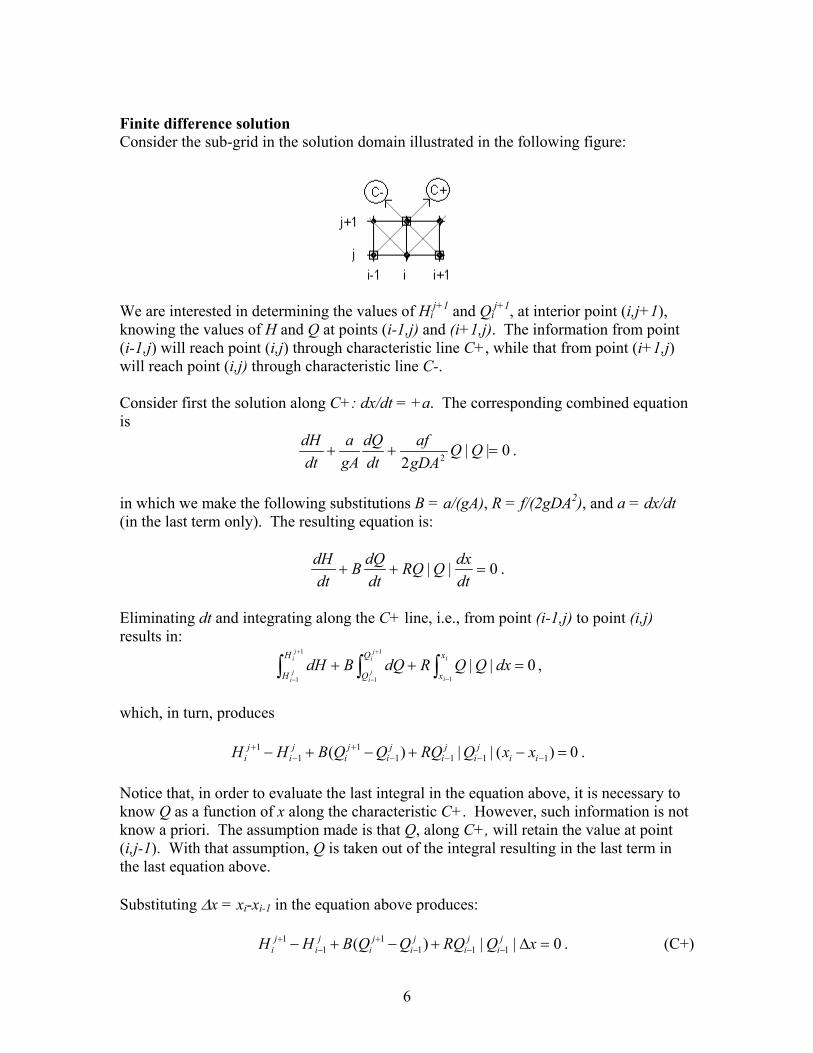
Finite difference solution Consider the sub-grid in the solution domain illustrated in the following figure:

We are interested in determining the values of Hi

j+1 and Qij+1, at interior point (i,j+1),

knowing the values of H and Q at points (i-1,j) and (i+1,j). The information from point (i-1,j) will reach point (i,j) through characteristic line C+, while that from point (i+1,j) will reach point (i,j) through characteristic line C-. Consider first the solution along C+: dx/dt = +a. The corresponding combined equation is

0||2 2 =++ QQ

gDAaf

dtdQ

gAa

dtdH .

in which we make the following substitutions B = a/(gA), R = f/(2gDA2), and a = dx/dt (in the last term only). The resulting equation is:

0|| =++dtdxQRQ

dtdQB

dtdH .

Eliminating dt and integrating along the C+ line, i.e., from point (i-1,j) to point (i,j) results in:

0||1

1

1

1

1

=++ ∫∫∫−

+

−

+

−

i

i

ji

ji

ji

ji

x

x

Q

Q

H

HdxQQRdQBdH ,

which, in turn, produces

0)(||)( 11111

11 =−+−+− −−−−

+−

+ii

ji

ji

ji

ji

ji

ji xxQRQQQBHH .

Notice that, in order to evaluate the last integral in the equation above, it is necessary to know Q as a function of x along the characteristic C+. However, such information is not know a priori. The assumption made is that Q, along C+, will retain the value at point (i,j-1). With that assumption, Q is taken out of the integral resulting in the last term in the last equation above. Substituting ∆x = xi-xi-1 in the equation above produces:

0||)( 1111

11 =∆+−+− −−−

+−

+ xQRQQQBHH ji

ji

ji

ji

ji

ji . (C+)

7

A similar analysis along C-: dx/dt = -a, requires us to use the combined equation:

0||2 2 =−− QQ

gDAaf

dtdQ

gAa

dtdH .

With B = a/(gA), R = f/(2gDA2), and a = - dx/dt (in the last term only), the combined equation becomes:

0|| =+−dtdxQRQ

dtdQB

dtdH .

Eliminating dt and integrating along the C- line, i.e., from point (i+1,j) to point (i,j) results in:

0||1

1

1

1

1

=++ ∫∫∫+

+

+

+

+

i

i

ji

ji

ji

ji

x

x

Q

Q

H

HdxQQRdQBdH ,

which, in turn, produces

0)(||)( 1111

1111 =−+−+− ++−+

+++

+ii

ji

ji

jji

ji

ji xxQRQQQBHH .

Here we use the assumption that Q, along C-, will retain the value at point (i,j+1). Substituting -∆x = xi – xi+1 in the equation above produces:

0||)( 111

1111 =∆−−+− +−+

+++

+ xQRQQQBHH ji

ji

jji

ji

ji . (C-)

Since the values at points (i-1,j) and (i+1,j) are known, the following constants can be identified in equations (C+) and (C-):

CP = || 1111j

ij

ij

ij

i QQxRBQH −−−− ⋅∆⋅−+ , and

CM = || 1111j

ij

ij

ij

i QQxRBQH ++++ ⋅∆⋅+− . With these constants, equations (C+) and (C-) become:

11 ++ ⋅−= ji

ji QBCPH , (C+)

and 11 ++ ⋅+= j

ij

i QBCMH . (C-). Notice that we have a system of two equations (C+,C-) in two unknowns Qi

j+1 and Hij+1.

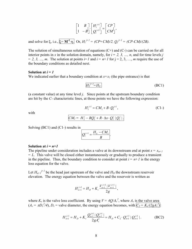
One way to solve the system is to write it as a matrix equation, M⋅ξ=η:

8

=

⋅

− +

+

CMCP

QH

BB

ji

ji

1

1

11

,

and solve for ξ, i.e., ξ= M-1⋅η. Or, Hi

j+1 = (CP+CM)/2, Qi j+1 = (CP-CM)/(2B).

The solution of simultaneous solution of equations (C+) and (C-) can be carried on for all interior points in x in the solution domain, namely, for i = 2, 3, …, n, and for time levels j = 2, 3, …, m. The solution at points i=1 and i = n+1 for j = 2, 3, …, m require the use of the boundary conditions as detailed next. Solution at i = 1 We indicated earlier that a boundary condition at x=x1 (the pipe entrance) is that

H1j+1=HU (BC1)

(a constant value) at any time level j. Since points at the upstream boundary condition are hit by the C- characteristic lines, at those points we have the following expression:

111

11

++ ⋅+= jj QBCMH , (C1-) with

CM1 = || 2222jjjj QQxRBQH ⋅∆⋅+− .

Solving (BC1) and (C1-) results in

BCMHQ Uj 11

1−

=+ .

Solution at i = n+1 The pipeline under consideration includes a valve at its downstream end at point x = xn+1 = L. This valve will be closed either instantaneously or gradually to produce a transient in the pipeline. Thus, the boundary condition to consider at point i = n+1 is the energy loss equation for the valve. Let Hn+1

j+1 be the head just upstream of the valve and HD the downstream reservoir elevation. The energy equation between the valve and the reservoir is written as

gVVKHH

jn

jn

vDj

n 2|| 1

11

111

++

+++

+ += ,

where Kv is the valve loss coefficient. By using V = 4Q/Av

2, where Av is the valve area (Av = πDv

2/4), Dv = valve diameter, the energy equation becomes, with C2 = Kv/(2gAv2):

||2

|| 11

1122

11

111

1++

++

++

+++

+ ⋅+=+= jn

jnD

v

jn

jn

vDj

n QQCHgA

QQKHH . (BC2)

9

Since point (n+1,j+1) is hit by characteristic C+, we also have the following equation available:

112

11

++

++ ⋅−= j

nj

n QBCPH , (C2+) with

CP2 = || jn

jn

jn

jn QQxRBQH ⋅∆⋅−+

From equations (BC2) and (C2+) we get a quadratic equation:

0||)( 211

11

112

11 =−+⋅+⋅= +

+++

++

++ CPHQBQQCQf D

jn

jn

jn

jn , (VEq)

which can be solved numerically. With the solution for Qn+1

j+1 from (VEq), equation (C2+) provides Hn+1

j+1. Notice that, once the valve is closed, you don’t need to solve equation (VEq) anymore. Simply take Qn+1

j+1 =0, and Hn+1 j+1 =CP2.

Valve loss coefficient The valve loss coefficient Kv (used in the energy equations involving the valve) can be obtained from the following equation in terms of a discharge coefficient Cd :

112 −=d

v CK . (VCEq)

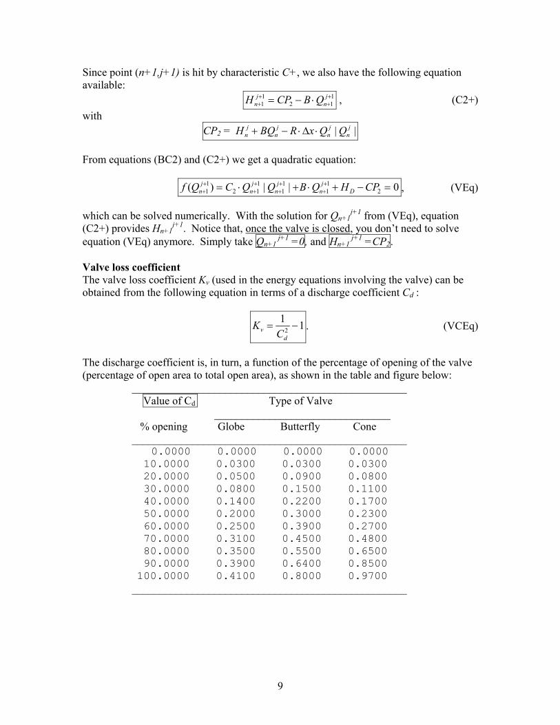
The discharge coefficient is, in turn, a function of the percentage of opening of the valve (percentage of open area to total open area), as shown in the table and figure below: __________________________________________________ Value of Cd Type of Valve ________________________________ % opening Globe Butterfly Cone __________________________________________________ 0.0000 0.0000 0.0000 0.0000

10.0000 0.0300 0.0300 0.0300 20.0000 0.0500 0.0900 0.0800 30.0000 0.0800 0.1500 0.1100 40.0000 0.1400 0.2200 0.1700 50.0000 0.2000 0.3000 0.2300 60.0000 0.2500 0.3900 0.2700 70.0000 0.3100 0.4500 0.4800 80.0000 0.3500 0.5500 0.6500 90.0000 0.3900 0.6400 0.8500 100.0000 0.4100 0.8000 0.9700

__________________________________________________

10

0 10 20 30 40 50 60 70 80 90 1000

0.1

0.2

0.3

0.4

0.5

0.6

0.7

0.8

0.9

1Discharge coefficient for different valve types

Valve opening (%)

Cd

Globe ButterflyCone

(Data from Fig. 4.3, page 91, in Tullis, J.P., 1989 , Hydraulics of Pipelines – Pumps, Valves, Cavitation, Transients, John Wiley & Sons, New York) Simulation of valve closing The closing of the valve can be simulated by letting the percentage valve opening (VO) decrease from its initial setting, say VOo (e.g., 50%, 75%), to VO = 0, in the time interval 0<t<tc, where tc = time to closure. Thus, VO(t) = VOo(1-t/tc). In the simulation, therefore, we should be able to calculate VO(tj), and, using linear interpolation, determine the discharge coefficient, Cd, from the table above. The calculation of Kv follows from Equation (VCEq), shown above. Data for simulation For the purpose of running a solution, utilize the following values (use Dv = D):

L D HU HD a tmax tc Valve Initial Case (ft) (ft) f (ft) (ft) (ft/s) (s) (s) type opening (%)

1 2000 1.00 0.000 50 0 1500 5 0 Cone 50% 2 2000 1.00 0.030 50 0 1500 50 0 Cone 50% 3 2000 1.00 0.030 50 0 1500 50 2.67 Cone 50% 4 17000 0.833 0.0123 750 200 1500 800 11.3 Butterfly 100% 5 17000 0.833 0.0123 750 200 1500 800 22.7 Butterfly 100% 6 17000 0.833 0.0123 750 200 1500 800 45.3 Butterfly 100% 7 17000 0.833 0.0123 750 200 1500 800 90.7 Butterfly 100% 8 17000 0.833 0.0123 750 200 1500 800 181 Butterfly 100% 9 17000 0.833 0.0123 750 200 1500 800 282 Butterfly 100% 10 17000 0.833 0.0123 750 200 1500 800 725 Butterfly 100%

In the table tc stands for the time of closure, i.e., the time at which the valve should be fully closed assuming a linear closure function. Thus, at t = 0, valve opening = initial setting (%), and at t = tc, valve opening = 0 %, in a linear fashion. The value tc = 0 corresponds to an instant closure, i.e., the valve is open for the first time step only, and closed afterwards.

11

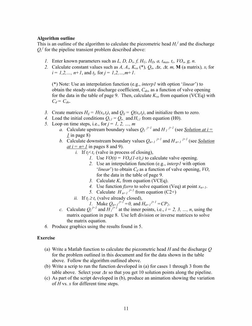
Algorithm outline This is an outline of the algorithm to calculate the piezometric head Hi

j and the discharge Qi

j for the pipeline transient problem described above:

1. Enter known parameters such as L, D, Dv, f, HU, HD, a, tmax, tc, VOo, g, n. 2. Calculate constant values such as A, Av, Kvo (*), Qo, ∆x, ∆t, m, M (a matrix), xi for

i = 1,2,…, n+1, and tj, for j = 1,2,…,m+1.

(*) Note: Use an interpolation function (e.g., interp1 with option ‘linear’) to obtain the steady-state discharge coefficient, Cdo, as a function of valve opening for the data in the table of page 9. Then, calculate Kvo from equation (VCEq) with Cd = Cdo.

3. Create matrices Hij = H(xi,tj), and Qij = Q(xi,tj), and initialize them to zero. 4. Load the initial conditions Qi,1 = Qo , and Hi,1 from equation (H0). 5. Loop on time steps, i.e., for j = 1, 2, …, m

a. Calculate upstream boundary values Q1 j+1 and H 1

j+1 (see Solution at i = 1 in page 8)

b. Calculate downstream boundary values Qn+1 j+1 and H n+1

j+1 (see Solution at i = n+1 in pages 8 and 9).

i. If tj<tc (valve in process of closing), 1. Use VO(t) = VOo(1-t/tc) to calculate valve opening. 2. Use an interpolation function (e.g., interp1 with option

‘linear’) to obtain Cd as a function of valve opening, VO, for the data in the table of page 9.

3. Calculate Kv from equation (VCEq). 4. Use function fzero to solve equation (Veq) at point xn+1. 5. Calculate H n+1

j+1 from equation (C2+) ii. If tj ≥ tc (valve already closed),

1. Make Qn+1 j+1 =0, and Hn+1

j+1 =CP2. c. Calculate Qi

j+1 and H i j+1 at the inner points, i.e., i = 2, 3, …, n, using the

matrix equation in page 8. Use left division or inverse matrices to solve the matrix equation.

6. Produce graphics using the results found in 5. Exercise

(a) Write a Matlab function to calculate the piezometric head H and the discharge Q for the problem outlined in this document and for the data shown in the table above. Follow the algorithm outlined above.

(b) Write a scrip to run the function developed in (a) for cases 1 through 3 from the table above. Select your ∆x so that you get 10 solution points along the pipeline.

(c) As part of the script developed in (b), produce an animation showing the variation of H vs. x for different time steps.

12

(d) Repeat the animation produced in (c) for the discharge Q vs. x for different time steps.

(e) For the data of cases 1 through 3, plot the variation of H vs. t, at three points along the pipeline: (1) the upstream boundary (i = 1), (2) the mid point (i = round(n/2)), and the upstream boundary (i = n+1). Plot the three signals in the same plot, identifying the different signals with the command legend.

(f) Plot the variation of Q vs. t for the same points listed in (e). Use a single plot, identifying the different signals with the command legend.

(g) Prepare a script to run the solution developed in (a) for cases 4 through 10 in the table above, and obtain the maximum head at the valve (Hv

max) for each case. Then, plot Hv

max vs. tc. Additional information on hydraulic transients Hydraulic transients are problems of practical applications in many hydraulic systems. The case presented here is a relatively simple case of a single pipeline, two reservoirs and a valve. More complicated cases may include two or more pipelines, branching pipelines, pipeline networks, free-flowing valves, pump failure, surge tanks, governed turbines, valve stroking, column separation (cavitation), oscillatory flow, etc. If interested in additional information about hydraulic transients, consult the following references: [1]. Chaudhry, M. H., 1979, Applied Hydraulic Transients, Van Nostrand Reinhold Co., New York [2]. Tullis, J.P., 1989 , Hydraulics of Pipelines – Pumps, Valves, Cavitation, Transients, John Wiley & Sons, New York [3]. Wylie, E.B. and V.L. Streeter, 1983, Fluid Transients, FEB Press, Ann Arbor, Michigan