Transient UWB Antenna Near-Field and Far-Field Assessment ...

HAL Id: hal-01242850https://hal-centralesupelec.archives-ouvertes.fr/hal-01242850

Submitted on 14 Dec 2015

HAL is a multi-disciplinary open accessarchive for the deposit and dissemination of sci-entific research documents, whether they are pub-lished or not. The documents may come fromteaching and research institutions in France orabroad, or from public or private research centers.

L’archive ouverte pluridisciplinaire HAL, estdestinée au dépôt et à la diffusion de documentsscientifiques de niveau recherche, publiés ou non,émanant des établissements d’enseignement et derecherche français ou étrangers, des laboratoirespublics ou privés.

Transient UWB Antenna Near-Field and Far-FieldAssessment From Time Domain Planar Near-Field

Characterization: Simulation and MeasurementInvestigationsMohammed Serhir

To cite this version:Mohammed Serhir. Transient UWB Antenna Near-Field and Far-Field Assessment From Time Do-main Planar Near-Field Characterization: Simulation and Measurement Investigations . IEEE Trans-actions on Antennas and Propagation, Institute of Electrical and Electronics Engineers, 2015, 63 (11),pp.4868-4876. �10.1109/TAP.2015.2480404�. �hal-01242850�

https://hal-centralesupelec.archives-ouvertes.fr/hal-01242850

https://hal.archives-ouvertes.fr

> REPLACE THIS LINE WITH YOUR PAPER IDENTIFICATION NUMBER (DOUBLE-CLICK HERE TO EDIT) <

1

Abstract— In this paper we present the experimental

validation of Time-Domain (TD) Near-Field to Near-Field

(NFNF) and Near-Field to Far-Field (NFFF) transformations for

UWB antenna transient characterization. The used computation

schemes for near-field to near- or far-field transformations are

based on the Green’s function representation of the radiated field

where NF and FF are directly calculated in the time domain. The

first step of the validation process comprises the electromagnetic

simulation results dedicated to evaluate the accuracy of NFFF

and NFNF transformations. The second step uses near-field

measurement data of a Vivaldi antenna to validate the developed

computation schemes whereas the measurement and calibration

procedures are fully described. The measured NF data using

Supelec planar and cylindrical near-field facilities are also

compared with the electromagnetic simulation transient results

of the Vivaldi antenna.

Index Terms— Time domain, antenna measurement, near-field

far-field transformation,

I. INTRODUCTION

OR Ground Penetrating Radar applications we are

interested in measuring the free space transient response of

Ultra Wide Band (UWB) antennas composing the radar [1][2].

The duration of the transient response is of a crucial

importance and the designers try to shorten the antenna free

space impulse response while enlarging its frequency

bandwidth of matched input impedance (S11<-10dB) [3].

More generally, GPR using UWB non-dispersive antennas

provides easily interpretable radargrams [4][5].

UWB antennas transient characterization can be carried out

using NF or FF techniques [6][7]. Based on the Huygens

principle, the NF measurement techniques make use of the

tangential components of electric or magnetic field collected

over a scan surface in the vicinity of the AUT. Then, these

measured data are transformed to calculate the

electromagnetic field at different distances [8]. The NF

measurements can be conducted in a small and low cost

Manuscript received February 19, 2015. M. Serhir is with Laboratoire Genie electrique et electronique de Paris

(GeePs) (UMR 8507 CentraleSupelec - CNRS – UPSud - UPMC) 11 rue

Joliot-Curie - Plateau de Moulon 91192 Gif sur Yvette Cedex - France, (e-mail: [email protected]).

anechoic chamber and by time-gating the measured data, one

can filter out multiple reflections occurring during the

measurement [9][10]. This allows the data accuracy

enhancement especially for low frequency measurement in

small anechoic chambers for which the absorption quality is

unsatisfactory. The TD techniques permit also the radiation

pattern measurement in non-anechoic environment as

presented in [11-14]. They are well adapted for studying the

parasitic electromagnetic radiation emitted from electronic

devices for electromagnetic compatibility purposes [15].

Even the theoretical development of the NFNF and NFFF

transformations are detailed in [6][16][17], the experimental

utilization of TD NF techniques are less popular than the FD

techniques. This is due to difficult experimental

implementation combined with the drawback related to the

computer time requirement, which could make unrealistic the

application of the technique to cases of practical interest. The

transient NF measurement systems use wideband and small

probes with low interaction with the AUT [18]. Moreover, in

NFNF and NFFF transformation schemes the measured E-

field and its time derivative are involved in the calculation

process. The accuracy of the NFNF and NFFF transformation

results depends on the highest point of the chosen

interpolation technique to keep working with the minimum

number of measured data [19]. In this paper, we use the

reconstruction formula to calculate and interpolate the E-field

and its time derivative as well for NFNF and NFFF

transformation schemes.

Here we aim at validating NFNF and NFFF transformations

using the experimental measurement and the electromagnetic

simulation software CST MWS [20]. An UWB Vivaldi

antenna designed for Ground Penetrating Radar (GPR) is used

for this purpose. The Vivaldi TD NF data are collected at

different distances from the antenna. First, the NFFF

transformation results are presented in order to outline the

errors due to the measurement surface truncation. Second, we

evaluate the accuracy of the NFNF calculation using different

set of measured NF data collected at different distances from

the AUT. Third, we present the experimental validation of the

NFNF transformation scheme we have developed based on the

Green’s function representation. Our algorithms are applied to

data obtained from the measurement of the Vivaldi antenna in

Transient UWB Antenna Near-Field and Far-

Field Assessment from Time-Domain Planar

Near-Field Characterization: Simulation and

Measurement Investigations

Mohammed Serhir, Member, IEEE

F


2

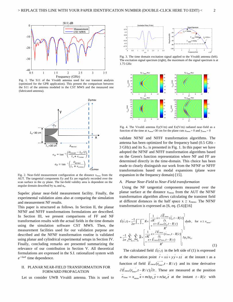
Fig. 3. The time domain excitation signal applied to the Vivaldi antenna (left).

The excitation signal spectrum (right), the maximum of the signal spectrum is at

1.75 GHz

Supelec planar near-field measurement facility. Finally, the

experimental validation aims also at comparing the simulation

and measurement NF results.

This paper is structured as follows. In Section II, the planar

NFNF and NFFF transformations formulations are described.

In Section III, we present comparisons of FF and NF

transformation results with the actual fields in the time domain

using the simulation software CST MWS. Then, the

measurement facilities used for our validation purpose are

described and the NFNF transformation routine is validated

using planar and cylindrical experimental setups in Section IV.

Finally, concluding remarks are presented summarizing the

relevance of our contribution in Section V. All theoretical

formulations are expressed in the S.I. rationalized system with

𝑒−𝑖𝜔𝑡 time dependence.

II. PLANAR NEAR-FIELD TRANSFORMATION FOR

FORWARD PROPAGATION

Let us consider UWB Vivaldi antenna. This is used to

validate NFNF and NFFF transformation algorithms. The

antenna has been optimized for the frequency band (0.5 GHz -

3 GHz) and its S11 is presented in Fig. 1. In this paper we have

adopted the NFNF and NFFF transformation algorithms based

on the Green's function representation where NF and FF are

determined directly in the time-domain. This choice has been

made to clearly distinguish our work from the NFNF or NFFF

transformations based on modal expansions (plane wave

expansion in the frequency domain) [15].

A. Planar Near-Field to Near-Field transformation

Using the NF tangential components measured over the

planar surface at the distance xmeas from the AUT the NFNF

transformation algorithm allows calculating the transient field

at different distances in the half space x ≥ xmeas. The NFNF

transformation is expressed as [6, eq. (5.6)][16]

meas

02

measmeas 0

3

meas0

2

0 0meas 0

3

1( , )1

( , ) , for .( , )2

1( , )1

,( , )2

Nz mn

mnm n Nz

Ex r t R c

cR tE r t R dydz x xx E r t R c

RE

x r t R ccR tR y z

x E r t R c

R

Ny

Ny

(1)

The calculated field ( , )E r t in the left side of (1) is expressed

at the observation point r xx y y zz at the instant t as a

function of field meas 0( , / )mnE r t R c and its time derivative

meas 0( , / )mnE r t R c t . These are measured at the position

0 meas 0 0mnr x x m y y n z z at the instant t R c with

Fig. 1. The S11 of the Vivaldi antenna used for our transient analysis

(optimized for the GPR application). This present the comparison between

the S11 of the antenna modeled in the CST MWS and the measured one

(fabricated antenna).

Fig. 2. Near-field measurement configuration at the distance xmeas from the

AUT. The tangential components Ey and Ez are regularly recorded over the

scan surface in the zy plane. The far-field validity area is dependent on the

angular domain described by αθ and αφ.

Fig. 4. The Vivaldi antenna Ey(V/m) and Ez(V/m) radiated near-field as a

function of the time at xmeas=30 cm for the plane cuts zmeas = 0 and ymeas = 0


3

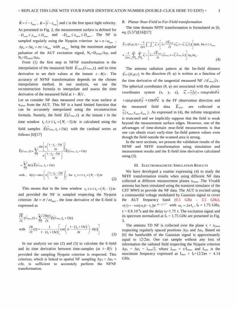
0mnR r r , 0mnR r r and c is the free space light velocity.

As presented in Fig. 2, the measurement surface is defined for

measymax ymaxD y D and measzmax zmaxD z D . The NF is

sampled regularly using the Nyquist criterion / maxt ,

0 0 / maxy z c with max being the maximum angular

pulsation of the AUT excitation signal, Ny=Dymax/Δy0 and

Nz=Dzmax/Δz0.

From (1) the first step in NFNF transformation is the

interpolation of the measured field meas 0( , )mnE r t and its time

derivative to set their values at the instant t R c . The

accuracy of NFNF transformation depends on the chosen

interpolation method. In our analysis, we use the

reconstruction formula to interpolate and assess the time

derivative of the measured field at t R c .

Let us consider NF data measured over the scan surface at

xmeas from the AUT. This NF is a band limited function that

can be accurately interpolated using the reconstruction

formula. Namely, the field 0( , )mnE r t at the instant t in the

time window 0 0 1tt t t N t is calculated using the

field samples 0 0( , )mnE r t l t with the cardinal series as

follows [6][17]

0

1

0 0 0

0 0

1

0 0

0

00 0

sin

( , ) ( , )

( ). ( , )

with , ( ) sin , for 1

t

t

N

mn mn

l

N

mn

l

t

t t l t

tE r t E r t l t

t t l t

t

h t E r t l t

t t l th t c t t t N t

t

(2)

This means that in the time window 0 0 1tt t t N t

and provided the NF is sampled respecting the Nyquist

criterion / maxt , the time derivative of the E-field is

expressed as

1

0 0 0

0

0

0

( )( , ) ( , )

1with ( ) cos ( )

( )

tN

mn mn

l

E h tr t E r t l t

t t

t t l tht h t

t t t l t t

(3)

In our analysis we use (2) and (3) to calculate the E-field

and its time derivative between time-samples (at t R c )

provided the sampling Nyquist criterion is respected. This

criterion, which is linked to spatial NF sampling Δy0 = Δz0 =

cΔt, is sufficient to accurately perform the NFNF

transformation.

B. Planar Near-Field to Far-Field transformation

The time domain NFFF transformation is formulated as [6,

eq. (5.57)][16][17]

meas

0 0 meas

meas0 0 0 0

1( , , ) ( , . ) , for

2

1( , . ) ,

2

FF r r

Ny Nz

mn mnr r

m Ny n Nz

EE t e x r t e r c dydz x x

c t

Ee x r t e r c y z

c t

(4)

The antenna radiation pattern at the far-field distance

, ,FFE t in the direction (θ, φ) is written as a function of

the time derivative of the tangential measured NF measE t .

The spherical coordinates (θ, φ) are associated with the planar

coordinates system (x, y, z), re r r cos sin x

sin sin y cos z is the FF observation direction and

the measured field data measE are collected at

0 meas meas meas, ,r x y z . As expressed in (4), the infinite integration

is truncated and we implicitly suppose that the field is weak

beyond the measurement surface edges. However, one of the

advantages of time-domain near-field measurements is that

one can obtain exact early-time far-field pattern values even

though the field outside the scanned area is strong.

In the next sections, we present the validation results of the

NFNF and NFFF transformation using simulation and

measurement results and the E-field time derivative calculated

using (3).

III. ELECTROMAGNETIC SIMULATION RESULTS

We have developed a routine expressing (4) to study the

NFFF transformation results when using different NF data

collected at different measurement planes xmeas .The Vivaldi

antenna has been simulated using the transient simulator of the

CST MWS to provide the NF data. The AUT is excited using

a cosinusoidal voltage modulated by Gaussian signal to cover

the AUT frequency band (0.5 GHz - 3.5 GHz),

2 2

04( )

0 0cos ( )t t

e t t t e

with 0 02 f , f0 = 1.75 GHz,

τ = 0.8.10-9s and the delay t0=1.75 τ. The excitation signal and

its spectrum normalized at f0 = 1.75 GHz are presented in Fig.

3.

The antenna TD NF is collected over the plane x = xmeas

respecting regularly spaced positions Δy0 and Δz0. Based on

[6] the bandwidth of the Gaussian signal is approximately

equal to 12/2πτ. One can sample without any loss of

information the radiated field respecting the Nyquist criterion

Δy0 = Δz0 = λmin/2, where λmin = c/fmax, and fmax is the

maximum frequency expressed as fmax = f0+12/2πτ = 4.14

GHz.


4

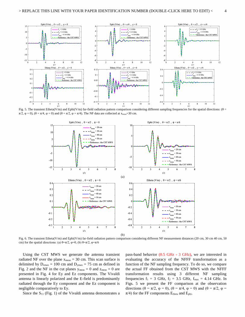
Using the CST MWS we generate the antenna transient

radiated NF over the plane xmeas = 30 cm. This scan surface is

delimited by Dzmax = 100 cm and Dymax = 75 cm as defined in

Fig. 2 and the NF in the cut planes ymeas = 0 and zmeas = 0 are

presented in Fig. 4 for Ey and Ez components. The Vivaldi

antenna is linearly polarized and the E-field is predominantly

radiated through the Ey component and the Ez component is

negligible comparatively to Ey.

Since the S11 (Fig. 1) of the Vivaldi antenna demonstrates a

pass-band behavior (0.5 GHz - 3 GHz), we are interested in

evaluating the accuracy of the NFFF transformation as a

function of the NF sampling frequency. To do so, we compare

the actual FF obtained from the CST MWS with the NFFF

transformation results using 3 different NF sampling

frequencies f1 = 3 GHz, f2 = 3.5 GHz, fmax = 4.14 GHz. In

Figs. 5 we present the FF comparison at the observation

directions (θ = π/2, φ = 0), (θ = π/4, φ = 0) and (θ = π/2, φ =

π/4) for the FF components Etheta and Ephi.

Fig. 5. The transient Etheta(V/m) and Ephi(V/m) far-field radiation pattern comparison considering different sampling frequencies for the spatial directions: (θ =

π/2, φ = 0), (θ = π/4, φ = 0) and (θ = π/2, φ = π/4). The NF data are collected at xmeas=30 cm.

(a)

(b)

Fig. 6. The transient Etheta(V/m) and Ephi(V/m) far-field radiation pattern comparison considering different NF measurement distances (20 cm, 30 cm 40 cm, 50

cm) for the spatial directions: (a) θ=π/2, φ=0, (b) θ=π/2, φ=π/6


5

As seen in Figs. 5 good agreements are noticed between the

Ephi (co-polar) component of the actual FF and the ones

resulting from NFFF transformations. The use of the sampling

frequency f1 = 3 GHz is responsible of the aliasing effects

clearly seen for the cross-polarization component Etheta. In

addition, the differences between the curves of Fig. 5 are due

to measurement surface truncation. For the far-field

observation point (θ = π/2, φ = 0) the difference between the

actual FF and the calculated one starts at t = 5.11τ that

corresponds to the arrival time when the center of the pulse

reached the measurement edge Dymax = 75 cm. The error

corresponding to the measurement edge Dzmax = 100 cm is

visible around t = 6.10τ.

Using the sampling frequency fmax = 4.14 GHz, we compare

the NFFF results calculated from NF data collected at different

planes xmeas = 20 cm, 30 cm, 40 cm, 50 cm. These calculated

FF are compared in Figs. 6 with the actual one at the

directions (θ = π/2, φ = π/6) and (θ = π/3, φ = 0). As presented

in Figs. 6, good agreements are noticed for 2.5τ ≤ t ≤ ttr, where

ttr depends on the measurement distance xmeas and the FF

observation point (θ, φ). This effect is known as the truncation

error and the FF reliable region is defined by αθ and αφ

expressed in Fig. 2 depends on the measurement distance.

Based on the presented simulation results, the developed

NFFF transformation routine has been validated using the

CST MWS. The NFFF transformation results have shown a

satisfactory accuracy while using the Nyquist criterion for NF

sampling.

The next comparisons aim at validating the TD NFNF

transformation routine. For this, we provide tangential NF data

at xmeas = 20 cm for -75 cm ≤ ymeas ≤ 75 cm and -100 cm ≤

zmeas ≤ 100 cm sampled using fmax = 4.14 GHz. Thereafter, we

perform the NFNF transformation routine to calculate the field

at 50 cm from the AUT. The NFNF transformation results

(ENFtoNF) are compared with the actual NF (Eref) at the plane

cuts (x = 50 cm, y = 0, -100 cm ≤ z ≤ 100 cm) and (x = 50 cm,

-75 cm ≤ y ≤ 75 cm, z = 0) using the error expressed as:

0 0 max max max max1 , ,

, , , ,, , 100

max , ,

t y y z z

NFtoNF ref

ref

t t t N t D y D D z D

E y z t E y z terror y z t

E y z t

. (8)

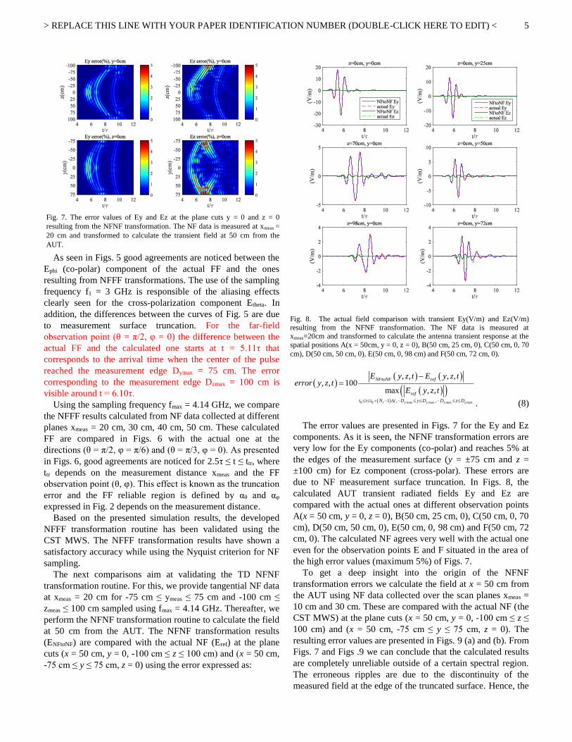
The error values are presented in Figs. 7 for the Ey and Ez

components. As it is seen, the NFNF transformation errors are

very low for the Ey components (co-polar) and reaches 5% at

the edges of the measurement surface (y = ±75 cm and z =

±100 cm) for Ez component (cross-polar). These errors are

due to NF measurement surface truncation. In Figs. 8, the

calculated AUT transient radiated fields Ey and Ez are

compared with the actual ones at different observation points

A(x = 50 cm, y = 0, z = 0), B(50 cm, 25 cm, 0), C(50 cm, 0, 70

cm), D(50 cm, 50 cm, 0), E(50 cm, 0, 98 cm) and F(50 cm, 72

cm, 0). The calculated NF agrees very well with the actual one

even for the observation points E and F situated in the area of

the high error values (maximum 5%) of Figs. 7.

To get a deep insight into the origin of the NFNF

transformation errors we calculate the field at x = 50 cm from

the AUT using NF data collected over the scan planes xmeas =

10 cm and 30 cm. These are compared with the actual NF (the

CST MWS) at the plane cuts (x = 50 cm, y = 0, -100 cm ≤ z ≤

100 cm) and (x = 50 cm, -75 cm ≤ y ≤ 75 cm, z = 0). The

resulting error values are presented in Figs. 9 (a) and (b). From

Figs. 7 and Figs .9 we can conclude that the calculated results

are completely unreliable outside of a certain spectral region.

The erroneous ripples are due to the discontinuity of the

measured field at the edge of the truncated surface. Hence, the

Fig. 7. The error values of Ey and Ez at the plane cuts y = 0 and z = 0

resulting from the NFNF transformation. The NF data is measured at xmeas =

20 cm and transformed to calculate the transient field at 50 cm from the

AUT.

Fig. 8. The actual field comparison with transient Ey(V/m) and Ez(V/m)

resulting from the NFNF transformation. The NF data is measured at xmeas=20cm and transformed to calculate the antenna transient response at the

spatial positions A(x = 50cm, y = 0, z = 0), B(50 cm, 25 cm, 0), C(50 cm, 0, 70

cm), D(50 cm, 50 cm, 0), E(50 cm, 0, 98 cm) and F(50 cm, 72 cm, 0).


6

entire calculated pattern is always affected by errors, and it is

not possible to define a region where the error is completely

zero. However, the concept of the spectral reliable far-field

region is usually applied to refer to the region in which the

error is not negligible but is low [21].

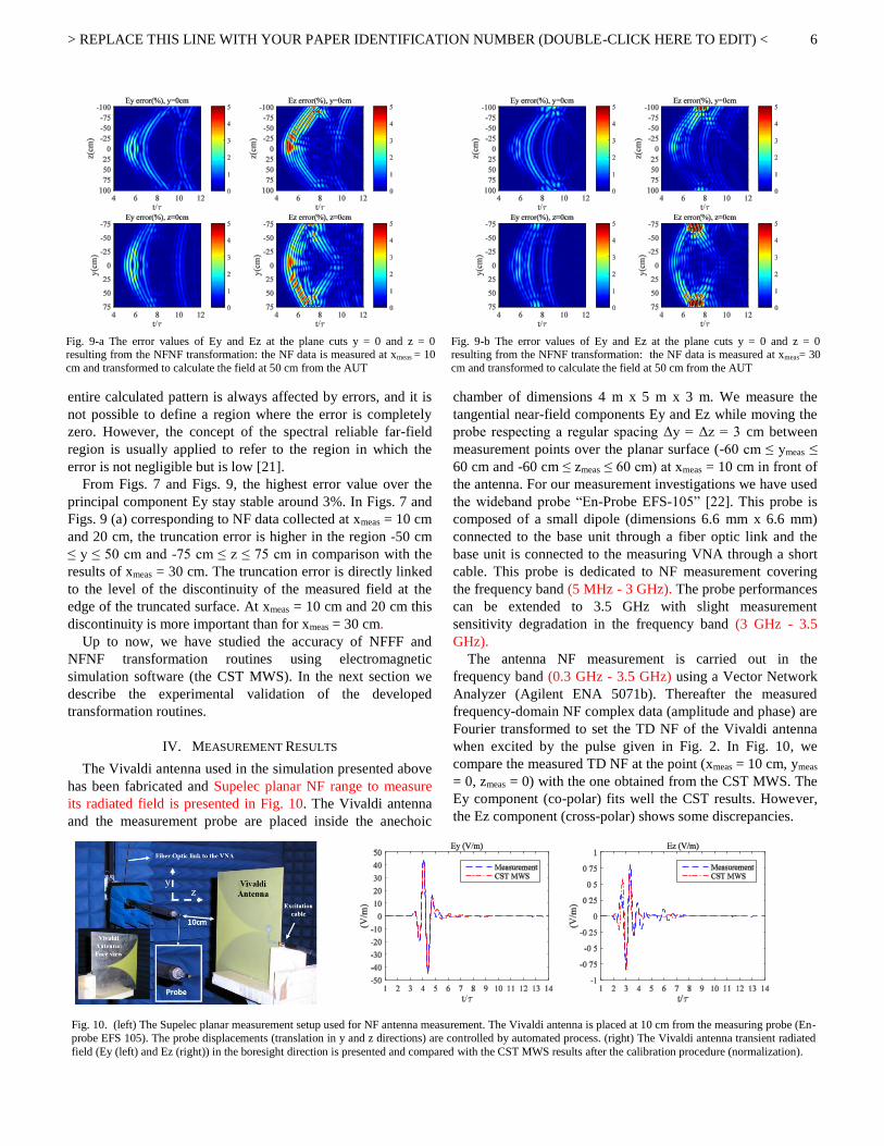
From Figs. 7 and Figs. 9, the highest error value over the

principal component Ey stay stable around 3%. In Figs. 7 and

Figs. 9 (a) corresponding to NF data collected at xmeas = 10 cm

and 20 cm, the truncation error is higher in the region -50 cm

≤ y ≤ 50 cm and -75 cm ≤ z ≤ 75 cm in comparison with the

results of xmeas = 30 cm. The truncation error is directly linked

to the level of the discontinuity of the measured field at the

edge of the truncated surface. At xmeas = 10 cm and 20 cm this

discontinuity is more important than for xmeas = 30 cm.

Up to now, we have studied the accuracy of NFFF and

NFNF transformation routines using electromagnetic

simulation software (the CST MWS). In the next section we

describe the experimental validation of the developed

transformation routines.

IV. MEASUREMENT RESULTS

The Vivaldi antenna used in the simulation presented above

has been fabricated and Supelec planar NF range to measure

its radiated field is presented in Fig. 10. The Vivaldi antenna

and the measurement probe are placed inside the anechoic

chamber of dimensions 4 m x 5 m x 3 m. We measure the

tangential near-field components Ey and Ez while moving the

probe respecting a regular spacing Δy = Δz = 3 cm between

measurement points over the planar surface (-60 cm ≤ ymeas ≤

60 cm and -60 cm ≤ zmeas ≤ 60 cm) at xmeas = 10 cm in front of

the antenna. For our measurement investigations we have used

the wideband probe “En-Probe EFS-105” [22]. This probe is

composed of a small dipole (dimensions 6.6 mm x 6.6 mm)

connected to the base unit through a fiber optic link and the

base unit is connected to the measuring VNA through a short

cable. This probe is dedicated to NF measurement covering

the frequency band (5 MHz - 3 GHz). The probe performances

can be extended to 3.5 GHz with slight measurement

sensitivity degradation in the frequency band (3 GHz - 3.5

GHz).

The antenna NF measurement is carried out in the

frequency band (0.3 GHz - 3.5 GHz) using a Vector Network

Analyzer (Agilent ENA 5071b). Thereafter the measured

frequency-domain NF complex data (amplitude and phase) are

Fourier transformed to set the TD NF of the Vivaldi antenna

when excited by the pulse given in Fig. 2. In Fig. 10, we

compare the measured TD NF at the point (xmeas = 10 cm, ymeas

= 0, zmeas = 0) with the one obtained from the CST MWS. The

Ey component (co-polar) fits well the CST results. However,

the Ez component (cross-polar) shows some discrepancies.

Fig. 10. (left) The Supelec planar measurement setup used for NF antenna measurement. The Vivaldi antenna is placed at 10 cm from the measuring probe (En-

probe EFS 105). The probe displacements (translation in y and z directions) are controlled by automated process. (right) The Vivaldi antenna transient radiated

field (Ey (left) and Ez (right)) in the boresight direction is presented and compared with the CST MWS results after the calibration procedure (normalization).

Fig. 9-a The error values of Ey and Ez at the plane cuts y = 0 and z = 0 resulting from the NFNF transformation: the NF data is measured at xmeas = 10

cm and transformed to calculate the field at 50 cm from the AUT

Fig. 9-b The error values of Ey and Ez at the plane cuts y = 0 and z = 0 resulting from the NFNF transformation: the NF data is measured at xmeas= 30

cm and transformed to calculate the field at 50 cm from the AUT


7

The NF probe used in this measurement campaign is

supposed to behave like a point source. For probe calibration

procedure, we have normalized the measured NF magnitude

(co-polar) in order to reach the CST MWS maximum NF

level. This is performed at the principal direction (xmeas = 10

cm, ymeas = zmeas = 0) and the normalization coefficient is

applied to measured NF data (Ey and Ez) over the

measurement surface.

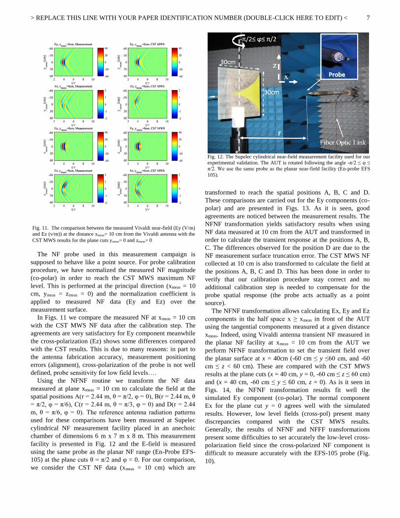
In Figs. 11 we compare the measured NF at xmeas = 10 cm

with the CST MWS NF data after the calibration step. The

agreements are very satisfactory for Ey component meanwhile

the cross-polarization (Ez) shows some differences compared

with the CST results. This is due to many reasons: in part to

the antenna fabrication accuracy, measurement positioning

errors (alignment), cross-polarization of the probe is not well

defined, probe sensitivity for low field levels….

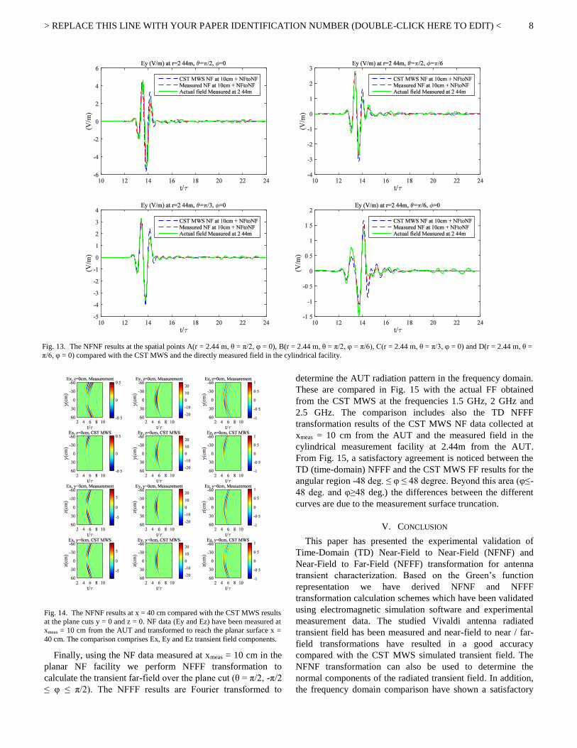
Using the NFNF routine we transform the NF data

measured at plane xmeas = 10 cm to calculate the field at the

spatial positions A(r = 2.44 m, θ = π/2, φ = 0), B(r = 2.44 m, θ

= π/2, φ = π/6), C(r = 2.44 m, θ = π/3, φ = 0) and D(r = 2.44

m, θ = π/6, φ = 0). The reference antenna radiation patterns

used for these comparisons have been measured at Supelec

cylindrical NF measurement facility placed in an anechoic

chamber of dimensions 6 m x 7 m x 8 m. This measurement

facility is presented in Fig. 12 and the E-field is measured

using the same probe as the planar NF range (En-Probe EFS-

105) at the plane cuts θ = π/2 and φ = 0. For our comparison,

we consider the CST NF data (xmeas = 10 cm) which are

transformed to reach the spatial positions A, B, C and D.

These comparisons are carried out for the Ey components (co-

polar) and are presented in Figs. 13. As it is seen, good

agreements are noticed between the measurement results. The

NFNF transformation yields satisfactory results when using

NF data measured at 10 cm from the AUT and transformed in

order to calculate the transient response at the positions A, B,

C. The differences observed for the position D are due to the

NF measurement surface truncation error. The CST MWS NF

collected at 10 cm is also transformed to calculate the field at

the positions A, B, C and D. This has been done in order to

verify that our calibration procedure stay correct and no

additional calibration step is needed to compensate for the

probe spatial response (the probe acts actually as a point

source).

The NFNF transformation allows calculating Ex, Ey and Ez

components in the half space x ≥ xmeas in front of the AUT

using the tangential components measured at a given distance

xmeas. Indeed, using Vivaldi antenna transient NF measured in

the planar NF facility at xmeas = 10 cm from the AUT we

perform NFNF transformation to set the transient field over

the planar surface at x = 40cm (-60 cm ≤ y ≤60 cm, and -60

cm ≤ z < 60 cm). These are compared with the CST MWS

results at the plane cuts (x = 40 cm, y = 0, -60 cm ≤ z ≤ 60 cm)

and (x = 40 cm, -60 cm ≤ y ≤ 60 cm, z = 0). As is it seen in

Figs. 14, the NFNF transformation results fit well the

simulated Ey component (co-polar). The normal component

Ex for the plane cut y = 0 agrees well with the simulated

results. However, low level fields (cross-pol) present many

discrepancies compared with the CST MWS results.

Generally, the results of NFNF and NFFF transformations

present some difficulties to set accurately the low-level cross-

polarization field since the cross-polarized NF component is

difficult to measure accurately with the EFS-105 probe (Fig.

10).

Fig. 11. The comparison between the measured Vivaldi near-field (Ey (V/m)

and Ez (v/m)) at the distance xmeas= 10 cm from the Vivaldi antenna with the

CST MWS results for the plane cuts ymeas= 0 and zmeas= 0

Fig. 12. The Supelec cylindrical near-field measurement facility used for our

experimental validation. The AUT is rotated following the angle -π/2 ≤ φ ≤

π/2. We use the same probe as the planar near-field facility (En-probe EFS

105).


8

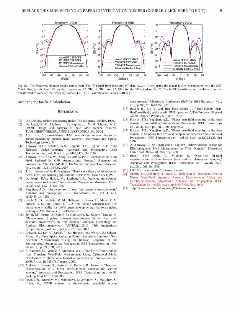
Finally, using the NF data measured at xmeas = 10 cm in the

planar NF facility we perform NFFF transformation to

calculate the transient far-field over the plane cut (θ = π/2, -π/2

≤ φ ≤ π/2). The NFFF results are Fourier transformed to

determine the AUT radiation pattern in the frequency domain.

These are compared in Fig. 15 with the actual FF obtained

from the CST MWS at the frequencies 1.5 GHz, 2 GHz and

2.5 GHz. The comparison includes also the TD NFFF

transformation results of the CST MWS NF data collected at

xmeas = 10 cm from the AUT and the measured field in the

cylindrical measurement facility at 2.44m from the AUT.

From Fig. 15, a satisfactory agreement is noticed between the

TD (time-domain) NFFF and the CST MWS FF results for the

angular region -48 deg. ≤ φ ≤ 48 degree. Beyond this area (φ≤-

48 deg. and φ≥48 deg.) the differences between the different

curves are due to the measurement surface truncation.

V. CONCLUSION

This paper has presented the experimental validation of

Time-Domain (TD) Near-Field to Near-Field (NFNF) and

Near-Field to Far-Field (NFFF) transformation for antenna

transient characterization. Based on the Green’s function

representation we have derived NFNF and NFFF

transformation calculation schemes which have been validated

using electromagnetic simulation software and experimental

measurement data. The studied Vivaldi antenna radiated

transient field has been measured and near-field to near / far-

field transformations have resulted in a good accuracy

compared with the CST MWS simulated transient field. The

NFNF transformation can also be used to determine the

normal components of the radiated transient field. In addition,

the frequency domain comparison have shown a satisfactory

Fig. 14. The NFNF results at x = 40 cm compared with the CST MWS results

at the plane cuts y = 0 and z = 0. NF data (Ey and Ez) have been measured at

xmeas = 10 cm from the AUT and transformed to reach the planar surface x =

40 cm. The comparison comprises Ex, Ey and Ez transient field components.

Fig. 13. The NFNF results at the spatial points A(r = 2.44 m, θ = π/2, φ = 0), B(r = 2.44 m, θ = π/2, φ = π/6), C(r = 2.44 m, θ = π/3, φ = 0) and D(r = 2.44 m, θ =

π/6, φ = 0) compared with the CST MWS and the directly measured field in the cylindrical facility.


9

accuracy for far-field calculation.

REFERENCES

[1] D.J. Daniels, Surface Penetrating Radar, The IEE press, London, 1996. [2] De Jongh, R. V., Ligthart, L. P., Kaploun, I. V., & Schukin, A. D.

(1999). Design and analysis of new GPR antenna concepts. TIJDSCHRIFT-NEDERLANDS ELEKTRONICA, 64, 26-32

[3] A.S. Turk, “Ultra-wideband TEM horn design antenna design for

ground-penetrating impulse radar systems”, Microwave and Optical Technology Letters, 41

[4] Yarovoy, A.G.; Schukin, A.D.; Kaploun, I.V.; Ligthart, L.P., "The

dielectric wedge antenna," Antennas and Propagation, IEEE Transactions on , vol.50, no.10, pp.1460,1472, Oct 2002

[5] Yarovoy, A.G.; Qiu, W.; Yang, B.; Aubry, P.J., "Reconstruction of the

Field Radiated by GPR Antenna into Ground," Antennas and

Propagation, 2007. EuCAP 2007. The Second European Conference on ,

vol., no., pp.1,6, 11-16 Nov. 2007

[6] T. B. Hansen and A. D. Yaghjian “Plane-wave theory of time-domain fields, near-field scanning applications” IEEE Press, New York (1999)

[7] De Jough, R.V.; Hajian, M.; Ligthart, L.P., "Antenna time-domain

measurement techniques," Antennas and Propagation Magazine, IEEE , vol.39, no.5, pp.7,11, Oct 1997

[8] Yaghjian, A.D., "An overview of near-field antenna measurements,"

Antennas and Propagation, IEEE Transactions on , vol.34, no.1, pp.30,45, Jan 1986

[9] Blech, M. D., Leibfritz, M. M., Hellinger, R., Geier, D., Maier, F. A.,

Pietsch, A. M., and Eibert, T. F.: A time domain spherical near-field measurement facility for UWB antennas employing a hardware gating

technique, Adv. Radio Sci., 8, 243-250, 2010.

[10] Serhir, M.; Picard, D.; Jouvie, F.; Guinvarc'h, R.; Ribiere-Tharaud, N., "Development of pulsed antennas measurement facility: Near field

antennas measurement in time domain," Antenna Technology and

Applied Electromagnetics (ANTEM), 2012 15th International Symposium on , vol., no., pp.1,4, 25-28 June 2012

[11] Jinhwan, K.; De, A.; Sarkar, T. K.; Hongsik, M.; Weixin, Z.; Salazar-

Palma, M., \Free Space Radiation Pattern Reconstruction from Non-Anechoic Measurements Using an Impulse Response of the

Environment," Antennas and Propagation, IEEE Transactions on , Vol.

60, No. 2, pp.821{ 831, 2012. [12] R. Rammal, M. Lalande, E. Martinod, et al., “Far-Field Reconstruction

from Transient Near-Field Measurement Using Cylindrical Modal

Development,” International Journal of Antennas and Propagation, vol. 2009, Article ID 798473, 7 pages, 2009.

[13] Andrieu, J.; Nouvet, S.; Bertrand, V.; Beillard, B.; Jecko, B., "Transient

characterization of a novel ultrawide-band antenna: the scissors antenna," Antennas and Propagation, IEEE Transactions on , vol.53,

no.4, pp.1254,1261, April 2005

[14] Levitas, B.; Drozdov, M.; Naidionova, I.; Jefremov, S.; Malyshev, S.; Chizh, A., "UWB system for time-domain near-field antenna

measurement," Microwave Conference (EuMC), 2013 European , vol.,

no., pp.388,391, 6-10 Oct. 2013 [15] Ravelo B., Liu Y. and Ben Hadj Slama J., "Time-domain near-

field/near-field transform with PWS operations", The European Physical

Journal Applied Physics, 53, 30701, 2011. [16] Hansen, T.B.; Yaghjian, A.D., "Planar near-field scanning in the time

domain .1. Formulation," Antennas and Propagation, IEEE Transactions

on , vol.42, no.9, pp.1280,1291, Sep 1994. [17] Hansen, T.B.; Yaghjian, A.D., "Planar near-field scanning in the time

domain .2. Sampling theorems and computation schemes," Antennas and

Propagation, IEEE Transactions on , vol.42, no.9, pp.1292,1300, Sep 1994.

[18] A. Yarovoy, R. de Jongh and L. Ligthart, "Ultrawideband sensor for

Electromagnetic Field Measurement in Time Domain," Electronics Letter, Vol. 36, No.20, 28th Sept. 2000

[19] Bucci, O.M.; D'Elia, G.; Migliore, D., "Near-field far-field

transformation in time domain from optimal plane-polar samples," Antennas and Propagation, IEEE Transactions on , vol.46, no.7,

pp.1084,1088, Jul 1998

[20] CST Microwave studio 2014 user’s guide. [21] Martini, E.; Breinbjerg, O.; Maci, S., "Reduction of Truncation Errors in

Planar Near-Field Aperture Antenna Measurements Using the

Gerchberg-Papoulis Algorithm," Antennas and Propagation, IEEE Transactions on , vol.56, no.11, pp.3485-3493, Nov. 2008.

[22] http://www.enprobe.de/products_FO-Antennas.htm.

Fig. 15. The frequency domain results comparison. The FF issued from measured NF data (xmeas= 10 cm) using the planar facility is compared with the CST MWS directly calculated FF for the frequencies 1.5 GHz, 2 GHz, and 2.5 GHz for the FF cut plane θ=π/2. The NFFF transformation results are Fourier

transformed to calculate the frequency domain FF. The FF validity area is about ± 48 deg.

Transient UWB Antenna Near-Field and Far-Field Assessment ...

Documents

Transcript of Transient UWB Antenna Near-Field and Far-Field Assessment ...