IET Generation, Transmission & Distribution

Research Article

Linear daily UC model to improve thetransient stability of power system

ISSN 1751-8687Received on 15th March 2018Revised 20th March 2019Accepted on 23rd April 2019doi: 10.1049/iet-gtd.2018.5102www.ietdl.org

Salar Naghdalian1, Turaj Amraee1 , Sadegh Kamali11Faculty of Electrical Engineering, K.N. Toosi University of Technology, Tehran, Iran

E-mail: amraee@kntu.ac.ir

Abstract: As coherency of generators decreases, the risk of rotor angle instability increases, especially under severecontingencies. The slow coherency as a network characteristic may be controlled by the locations of committed generators. Unitcommitment (UC) problem is conventionally carried out regarding operational and network constraints. In this study, a two-stepstrategy is developed to promote the slow coherency via the network constrained UC (NCUC) model on a daily horizon. First,conventional NCUC is executed. The most important generators with both economic and coherency merits are then determinedas representative generators. In the second step, the Slow Coherency Based Unit Commitment (SCBUC) is re-optimisedaccording to the results obtained from the first step, using a multi-objective function. The first part of the multi-objectivefunction is devoted to the cost of generation, start-up, and shutdown of generators. The goal of the second part of the multi-objective function is to maximise the coherency between the committed generators to reach a transient stability margin. Theproposed model is converted to a mixed integer linear programming model. The performance of the proposed method ofpromoting transient stability is investigated using the dynamic IEEE 118-bus test system.

 NomenclatureSets and subscripts

t index for timei, j index for bus numberw index for each segment of linearised functionΩb set of all busesΩg set of generator busesΩS set of representative generatorsΩT set of hours in study horizonΩW set of linearised segments

⋅ pc subscript for the generation cost⋅ sc subscript for the start-up cost⋅ sd subscript for the shutdown cost⋅ max maximum value of a given variable⋅ min minimum value of a given variable

Parameters

ai, bi, ci coefficients of the generation cost functionCi

SUp start-up cost of generator i

CiSDn shutdown cost of generator i

Riup ramp-up limit of generator i

Ridn ramp-down limit of generator i

UTion minimum up-time of generator i

DTioff minimum down-time of generator i

Pimax/Pi

min maximum/minimum active power limits of generator iQi

max/Qimin maximum/minimum reactive power limits of

generator iADi

t /RDit active/reactive demands for bus i at time t

Bwi power generation at the start of the segment wSwi slope of the segment w in the linearised cost functionGi j/Bi j real/image parts of admittance matrix between bus i

and bus jRSR

t required amount of spinning reserve at time tRi

max maximum available reserve related to generator i

FLi j maximum active flow of transmission line linking busi and bus j

SEDi, st electrical distance between generator i and the

representative unit s at time tHi inertia time constant of generator i

Variables

uit binary variable for on/off statuses of generator i at time

tpi

t /qit active/reactive generation of bus i at time t

vit∠θi

t voltage phasor of bus i at time t

Xi, ton number of continuous hours that generator i has been

on at time tXi, t

off number of continuous hours that generator i has beenoff at time t

Rit spinning reserve by generator i at time t (i ∈ Ωg)

λiwt length of power segment w at time t for cost function

of generator iyi

t auxiliary variable for linearising cost function ofgenerator i at time t

αit, βi

t, γit auxiliary variables for linearising minimum up-time

constraints of generator i at time tξi

t, ηit, μi

t auxiliary variables for a linearising minimum down-time constraints of generator i at time t

ks l slope of the lth piecewise linear block of (θi jt )2

Δθi jt l length of an lth piecewise linear block of θi j

t

θi jt + , θi j

t − positive variables as replacement of θi jt

ωi rotor speed of generator iLi, s

t auxiliary variable in linearising coherency constraintbetween generator i and representative unit s at time t

DVi, st binary variable used to specify the electrical distance

of generator i from its representative generator

1 IntroductionUnit commitment (UC) is a fundamental problem in power systemsoptimal scheduling, whose primary goal is to determine the on/offstatuses and economic dispatch of generating units in a daily orweekly horizon [1]. The main objective in the UC problem usually

IET Gener. Transm. Distrib.© The Institution of Engineering and Technology 2019

1

is the minimisation of generation cost, start-up cost, and emissioncost. This problem encompasses various operational and securityconstraints. Network constraints are an imperative part of the UCproblem [1, 2]. Network constraints mostly focus on the fulfilmentof steady-state conditions using AC power flow constraints.

In recent years, by increasing the penetration level of lowinertia distributed generation technologies, several models havebeen proposed to include the transient stability in power systemstudies. Two approaches are utilised for transient stabilityenhancement in operational studies such as UC programme. In thefirst approach, the transient stability is considered using time-domain simulations or transient energy functions in theoptimisation model of the power system operation studies. Insimulation-based methods, it is required to solve the discretisednon-linear swing equations along with the steady-state model of theoriginal network constrained unit constrained (NCUC) model.Also, the digital power system simulators can be utilised to assessthe transient stability as well as to determine the critical and non-critical generators using extended equal area criterion (EEAC)method. Also in the energy function method, it is required to definea suitable transient energy function over the system state variablessuch as speed and rotor angles of generators. Although the firstapproach methods are valuable; however, due to the computationalcomplexity of discretised swing equation, the efficiency of thetransient stability constrained (TSC) NCUC model remains a majorproblem. In the second approach, the transient stability assessmentis not directly included inside the optimisation model of NCUC.Instead, an index is introduced to promote the transient stability ofthe power system, indirectly. In this regard, the second approachmay be interpreted as an alternative for improving the transientstability in the UC study. In this research, the transient stability ofthe UC problem is improved indirectly using the coherencycriterion. The transient stability is improved based on theincreasing slow coherency criterion.

Transient stability has been considered in the optimal powerflow (OPF) model [3–6]. In TSC-OPF studies, the optimalgeneration of generating units are determined in such a way that aminimum critical clearing time (CCT) is preserved withoutconsidering the on/off statuses of generating units. In [7], adecomposition-based approach has been developed to consider thetransient stability in security constrained UC model using EEAC.Also, the digital power system simulator has been utilised toidentify the critical and non-critical generators. Similar work hasbeen done in [7]. In [8], an augmented Lagrange relaxation methodhas been utilised to solve the TSC-OPF as a sub-problem of the UCprogramme. Also in [8], a reduced space interior point method hasbeen utilised to solve the TSC-OPF sub-problem directly. In recentyears, the integration of renewable energy resources such as windpower has created more complexities in UC models of modernpower systems [9]. In [10–12], frequency stability constraints havebeen proposed to fulfil the safety of system frequency response. Inprevious proposed TSC UC models, the transient stabilityassessment is done directly using the swing equation with somesimplification using EEAC method or a digital power systemsimulator. Less effort has been done to improve the transientstability of Security Constrained Unit Commitment modelindirectly.

Slow coherency between synchronous generators is a physicalconfirmation of a weak connection. As coherency of generatorsincreases, the risk of rotor angle instability in power systemdecreases [13]. The coherency between synchronous generatorsdepends on the network characteristics as well as the relativelocations of generators. Therefore, the coherency of generators isaffected by the unit scheduling and their dispatch. In [14], it hasbeen shown that the grid structure especially the electricaldistances among the generator internal buses has a great impact onpower system dynamics.

In a power system, the generators with similar dynamicresponses are called coherent units [15]. In addition to enhancingtransient stability margin [13, 15], increasing the coherency ofgenerators has a great effect on mitigating low-frequency powerswings, especially in islanding conditions [16]. In previous studies,

no effort has been done to promote the slow coherency via thedaily unit scheduling.

In the literature, several approaches including model-based andmeasurement-based methods have been presented to discern thecoherency of generators [13]. The model-based methods mainlyrely on modal analysis. Hence, they are not suitable for the UCproblem, due to the high computational burden. Since UC is an off-line task, the measurement-based methods are not applicable to theUC problem too. In [14], it has been shown that the electricaldistance between generators has a great impact on dynamicinteractions between generators.

In this paper, a two-step strategy is developed to improve theslow coherency of synchronous generators in daily scheduling ofgenerating units. In the first step, the conventional NCUC model issolved. The coherency of committed generators is then determinedusing a coherency index. According to the obtained coherency andeconomic merits, for each area, a generator is selected as therepresentative generator of that area. In the second step, the SlowCoherency Based Unit Commitment (SCBUC) is optimised whilethe coherency is integrated inside the NCUC using the electricaldistance criterion. An iterative-based process is considered todetermine the weighting factors until providing target minimumCCT. The desired minimum CCT is considered as the stoppingcriterion for coherency improvement. To promote thecomputational efficiency of the proposed method, the SCBUCalong with the AC power balance constraints are linearised andsolved using CPLEX algorithm. The main contributions of thispaper are two-fold:

• Developing an analytic framework to promote the slowcoherency of the network via a two-step SCBUC model.

• Providing the transient stability margin indirectly using thecoherency concept.

• Providing an iterative-based approach for adjusting weightingfactors of the proposed multi-objective function to reach thetarget minimum CCT.

• Developing a mixed integer linear programming (MILP) modelfor the proposed SCBUC model to assure the optimality of theobtained schedule.

Regarding the flowchart shown in Fig. 1, the structure of theproposed two-step strategy is described. The first step of theproposed strategy contains some subsequent stages as follows:

• Executing the MILP model of NCUC programme withoutconsidering the coherency constraint, as described in Section 2and using (5) and (7)–(32).

• Determining the representative generator in each region asdescribed in Section 3.1, using (33) and (34).

• Constructing the electrical distance matrix using data obtainedfrom the NCUC model as described in Section 3.2, formulatedin (35) and (36).

The second step of the proposed strategy acts based on someuseful information obtained from the first step as follows:

• Constructing the objective functions of the proposed SCBUCincluding the operational cost of generators and coherency-based objective function as described in Sections 3.3 and 4,using (37)–(44).

• Optimising the multi-objective MILP-based SCBUC model anddoing time-domain simulations.

• Adjusting the ratio of weighting factors [i.e. (ρ1/ρ2)] in aniterative-based process as described in Section 4, to achieve thetarget minimum CCT.

The goal of the first step of the proposed strategy is determiningthe representative generators using the results obtained fromconventional NCUC model, and finally constructing the electricaldistance matrix. The goal of the second step of the strategy is toformulate the multi-objective SCBUC including the operationalcost and coherency of generators and adjusting weighting factors to

2 IET Gener. Transm. Distrib.© The Institution of Engineering and Technology 2019

reach the target minimum CCT based on an iterative process. Therest of this paper is organised as follows. In Section 2, the non-linear and linear formulations of the NCUC model is presented. InSection 3, the formulation of the slow coherency criterion as themost notable innovation of this work is described. In Section 4, themulti-objective function of the proposed SCBUC is presented andthe iterative-based process to reach the target minimum CCT isintroduced. The simulation results on a modified IEEE 118-bus testsystem are presented in Section 5. Finally, this paper is concludedin Section 6.

2 Linear formulation of the NCUC problemThe non-linear forms of the objective function and the operationalconstraints of units could be found in [1]. Network constraintsincluding load flow [i.e. (1) and(2)], bus voltage limits and lineflow limits [i.e. (3) and (4)] are applied for each bus i ∈ Ωb ateach time t ∈ ΩT. In load flow equations [i.e. (1) and (2)], thevariables pi

t, qit are fixed to zero in load buses. The reserve

requirement [i.e. (5)] is defined for the entire network and each unit

pitui

t − ADit = ∑

j ∈ Ωb

VitV j

t Gi j cos θi jt + Bi j sin θi j

t(1)

qitui

t − RDit = ∑

j ∈ Ωb

VitV j

t Gi jsin θi jt − Bi jcos θi j

t(2)

Vi, tmin ≤ Vi

t ≤ Vi, tmax (3)

−FLi j ≤ (Vit)2Gi j − Vi

tV jtGi j cos θi j

t − VitV j

tBi j sin θi jt ≤ FLi j (4)

∑i ∈ G

Rit ≥ RSR

t , Rit ≤ Pi

maxuit − Pi

t , Rit ≤ Ri

max(5)

The thermal limit of a given transmission line can be expressedbased on the maximum ampere capacity or maximum active power.Since in this paper, the power flow model has been expressedbased on the standard active and reactive power formulations, thethermal limits of transmission lines are expressed based on themaximum allowable active flow. Additionally, the thermal limits oftransmission lines in most of IEEE benchmark test grids such as

IEEE 118-bus test system are available based on the maximumactive power flow limits.

2.1 Objective function

The objective function of the NCUC problem conventionallyincludes the generation cost, start-up cost, and shutdown cost ofunits over a daily horizon. This objective function is linearisedusing (6)–(14). The auxiliary binary variable yi

t = uitui

t − 1 is definedfor linearising the cost function. The expression given in (6) refersto the generation cost of thermal units at the minimum allowedpower generation. For each generator, the limit of active power issegmented by (7). The slope of each segment in the utilisedpiecewise linearising method is determined by (8). The length ofeach power segment is limited by (9). There are various approachesto linearise the start-up and shutdown costs [17, 18]. Here, thestart-up and shutdown costs are linearised by (13) and (14),respectively

f pc Pimin = CiPi

min 2 + biPimin + ai, ∀i ∈ Ωg (6)

Bwi = pimin + (pi

max − pimin) w

N , ∀w ∈ ΩW, ∀i ∈ Ωg (7)

Swi = f pc τwi − f pc τ w − 1 iBwi − B w − 1 i

, B0i = pimin, ∀w ∈ ΩW, ∀i ∈ Ωg

(8)

0 ≤ λiwt ≤ (Bwi − B w − 1 i)ui

t, ∀w ∈ ΩW, ∀i ∈ Ωg, ∀t ∈ ΩT (9)

f pc pti = ui

tpimin + ∑

w ∈ NSwiλiw

t , ∀i ∈ Ωg, ∀t ∈ ΩT (10)

− 1 − uit − 1 ≤ ui

t − yit ≤ 1 − ui

t − 1 , ∀i ∈ Ωg, ∀t ∈ ΩT (11)

0 ≤ yit ≤ ui

t − 1, ∀i ∈ Ωg, ∀t ∈ ΩT (12)

f sc uit = (ui

t − yit)Ci

SUP, ∀i ∈ Ωg, ∀t ∈ ΩT (13)

f sd uti = (ui

t − 1 − yit)Ci

SDn, ∀i ∈ Ωg, ∀t ∈ ΩT (14)

2.2 Operational constraints

2.2.1 Ramping constraints: The non-linear forms of theramping-up and ramping-down constraints are discussed in [1].Using the auxiliary binary variable yi

t, the linear form of rampingconstraints are expressed as given in (15) and (16) for each uniti ∈ Ωg at each time t ∈ ΩT, respectively

pit − pi

t − 1 ≤ 1 − uit + yi

t RiUP + (ui

t − yit)Pi

min (15)

pit − 1 − pi

t ≤ 1 − uit − 1 + yi

t RiDn + (ui

t − 1 − yit)Pi

min (16)

2.2.2 Power production limits: The active and reactive powergenerations of each generator is limited by its physicalcharacteristics, which are given by the manufacturer. Theseconstraints are formulised by the equations below:

Piminui

t ≤ pit ≤ Pi

maxuit, ∀i ∈ Ωg, ∀t ∈ ΩT (17)

Qiminui

t ≤ qit ≤ Qi

maxuit ∀i ∈ Ωg, ∀t ∈ ΩT (18)

2.2.3 Minimum up-time limit: Owing to technical reasons, eachgenerator must be on/off for a specific number of hours after astart/shutdown action. The auxiliary variables βi

t = Xi, t − 1on ui

t − 1,αi

t = Xi, t − 1on ui

t , and γit = Xi, t − 1

on yit are, respectively, linearised by (19),

(20); (21), (22); and (24), (25). The minimum up-time equations

Fig. 1  Flowchart of the proposed two-step strategy

IET Gener. Transm. Distrib.© The Institution of Engineering and Technology 2019

3

then linearised using (23) and (26), for each unit i ∈ Ωg at eachtime t ∈ ΩT, respectively

− 1 − uit − 1 M ≤ Xi, t − 1

on − βit ≤ 1 − ui

t − 1 M (19)

0 ≤ βit ≤ ui

t − 1M (20)

− 1 − uit M ≤ Xi, t − 1

on − αit ≤ 1 − ui

t M (21)

0 ≤ αit ≤ ui

tM (22)

βit − UTi

onuit − 1 − αi

t + UTionui

t ≥ 0 (23)

− 1 − yit M ≤ Xi, t − 1

on − γit ≤ 1 − yi

t M (24)

0 ≤ γit ≤ yi

tM (25)

Xi, ton = ui

t + γit (26)

2.2.4 Minimum down-time limit: To linearise the minimumdown-time constraints, the auxiliary variables ξi

t = Xi, t − 1off ui

t − 1,ηi

t = Xi, t − 1off ui

t , and μit = Xi, t − 1

off yit are utilised and the process of

linearisation of minimum down-time equations is the same asminimum up-time equations. The minimum down-time constraintsthen linearised using (27) and (28), for each unit i ∈ Ωg at eachtime ∈ ΩT, respectively

ηit − DTi

offuit − ξi

t + DTioffui

t − 1 ≥ 0 (27)

Xi, toff = 1 + Xi, t − 1

off − ξit − ui

t − ηit + μi

t (28)

2.3 Linearising AC power flow equations

A combinatorial techniques relying on Taylor series expansion andutilising binary variables are utilised to linearise the AC powerflow equations. The non-linear terms of power flow equationsgiven by (1) and (2) are replaced by the simplified approximationrelying on Taylor series expansion as given in Table 1. It is notedthat the approximations are determined at the normal operationalpoint (i.e. Vi

t = 1, V jt = 1, θi j

t = 0). The linearising techniqueincluding auxiliary binary variables, as discussed in [19], isemployed to linearise the term θi j

t2. According to the constraintsgiven in (17) and (18), the linearised form of the AC load flowequations can be formulised as follows:

pit − ADi

t = 2Vit − 1 Gii + ∑

j ∈ Ωg & j ≠ iGi j(Vi

t + V jt

− 12 ∑

l ∈ Lks l Δθi j

t l − 1) + Bi jθi jt

(29)

qit − RDi

t = − (2Vit − 1)Bii − ∑

j ∈ Ωg & j ≠ iGi jθi j

t − Bi j Vit + V j

t

− 12 ∑

l ∈ Lks l Δθi j

t l − 1(30)

where θi jt = θi j

t + − θi jt − and ∑l ∈ L Δθi j

t (l) = θi jt + + θi j

t − . The slope ofeach segment is determined by the equation below:

ks(l) = (2 l − 1) θi jmax

L(31)

Accordingly, the non-linear expression of active line flow givenin (4) is linearised for each line from bus i to bus j as given in theequation below:

−FLi j ≤ 2Vit − 1 Gi j − Gi j Vi

t + V jt − 1

2 ∑l ∈ L

ks l Δθi jt l − 1

−Bi j(θi jt ) ≤ FLi j

(32)

3 Coherency evaluation indexThe aim of modelling presented in this section is to extract thecriterion which can be used to increase the coherency betweengenerators and improve the transient stability margin indirectly.The electrical distance between the internal nodes of generators hasa great impact on their dynamic interactions and coherency [14].Also in [20, 21], the electrical distance between generators hasbeen considered as a measure of their coherency. The main purposeof the proposed SCBUC model is to increase the coherency ofsynchronous machines to reach a minimum CCT as the transientstability margin. Coherency is measured between each pair ofgenerators. In this paper, the coherency of each generator ismeasured with respect to the centre-of-inertia (COI) reference. Inthis regard, the generator with the highest coherency with the COIreference is selected as the representative generator. The SCBUCproblem is solved in such a way that the electrical distance betweenthe committed units and the representative unit in each region isminimised. The coherency constraint is considered in SCBUCmodel based on the procedure given in Sections 3.1–3.3.

3.1 Determining representative generator in each region

For modelling the slow coherency in NCUC problem using theelectrical distance reduction method, representative generatorsshould be considered to measure the electrical distance in eacharea. Therefore, representative generators are determined as areference to measure the electrical distance in each area. Therepresentative generators have two important features. First, theyhave economical merits (e.g. committed in all times based on theconventional NCUC). Second, they have a maximum rotor speedcorrelation with COI rotor speed of their specified coherent area.Indeed, representative generators are generators with high inertiaso the impact of minor changes of network topology in the processof selecting these representative generators is not significant andrepresentative generators are selected with a reasonableapproximation.

The boundary of each region is selected based on the slowcoherency technique proposed in [16]. Now, for each region, arepresentative generator is determined as follows:

• Executing the conventional NCUC programme, withoutconsidering the coherency constraint.

• Calculating the speed of the COI using (31)

ωCOI =∑i = 1

n Hiωi

∑i = 1n Hi

(33)

• Calculating the correlation between the speed of committedgenerators (e.g. generators i) and the speed of the COI in eachregion using the equation below:

CRi(COI)

=n∑t = 1

n ωi t ωCOI t − ∑t = 1n ωi t × ∑t = 1

n [ωCOI(t)]A × B

(34)

Table 1 Taylor expansion of non-linear terms in power flowequationsNon-linearfunction

Taylor expansionformulation

Simplifiedformulation

VitV j

t cos θi jt Vi

t + V jt + cos θi j

t − 2Vi

t + V jt −

θi jt 2

2 − 1

VitV j

t sin θi jt sin θi j

t θi jt

(Vit)2 2Vi

t − 1 2Vit − 1

4 IET Gener. Transm. Distrib.© The Institution of Engineering and Technology 2019

A = n∑t = 1

nωi t 2 − ∑

t = 1

nωi t

2

B = n∑t = 1

n(ωCOI t )2 − ∑

t = 1

nωCOI(t)

2

• Selecting the generators with maximum correlation coefficientand economic priority (i.e. committed in all times usingconventional NCUC), as the representative generator in eachgroup.

3.2 Constructing electrical distance matrix

To calculate the electrical distance between generating units andthe representative generator, the modified Zbus (i.e. Zmodi j

t )including load model and synchronous reactance of generators isnow constructed. The reactances of the generators and their step-uptransformers are added to the relevant array in Zbus matrix. Themodified Zbus is calculated according to the equation below:

Zmodi, st = Zi, s

t + Xdi + XTr

i + (Xds + XTr

s ) (35)

The electrical distance between a given unit i and therepresentative unit s is considered as the coherency index

SEDi, st = Zmodi, s

t (36)

3.3 Objective function of slow coherency

The aim of the proposed objective function is to minimise theoperational cost and electrical distance (i.e. maximising coherencyto enhance transient stability) simultaneously. In the following, thecoherency constraints are formulated based on the electricaldistance matrix.

The coherency constraints are presented in (37)–(40). The totalcost of coherency (i.e. the electrical distance) of the committedgenerators can be calculated by (41). According to the constraintsgiven in (37)–(40), if a generator is online, its electrical distancefrom the related representative generator should be computed.Otherwise, it should not be included in the objective function

DVi, st − 1 ≤ ui

t − Li, st ≤ 1 − DVi, s

t , ∀i ∈ Ωg, ∀t ∈ ΩT, ∀s∈ ΩS

(37)

0 ≤ Li, st ≤ DVi, s

t ∀i ∈ Ωg, ∀t ∈ ΩT, ∀s ∈ ΩS (38)

∑s ∈ ΩS

DVi, st = 1, ∀i ∈ Ωg, ∀t ∈ ΩT (39)

CEDi, st = Li, s

t SEDi, st , ∀i ∈ Ωg, ∀t ∈ ΩT, ∀s ∈ ΩS (40)

CCF = ∑t ∈ ΩT

∑i ∈ Ωg

∑s ∈ ΩS

CEDi, st , ∀i ∈ Ωg, ∀t ∈ ΩT, ∀s

∈ ΩS(41)

4 Multi-objective MILP-based SCBUC modelThe weighted summation of the normalised values of bothobjectives is introduced as the objective function [22]. The twoobjectives are normalised by (42), in which the operational cost(i.e. F1) and the cost of coherency (i.e. F2) are expressed as givenby (43) and (44)

Z = ∑i = 1

2ρi

Fi x − Fimin

Fimax − Fi

min (42)

F1 = ∑t ∈ ΩT

∑i ∈ Ωg

(uitpi

min + ∑w ∈ ΩW

Swiλiwt )

+ ∑t ∈ ΩT

∑i ∈ Ωg

(uit − yi

t)CiSUP + ∑

t ∈ ΩT∑

i ∈ Ωg

(uit − 1 − yi

t)CiSDn

(43)

F2 = ∑t ∈ ΩT

∑i ∈ Ωg

∑s ∈ ΩS

CEDi, st

(44)

Each normalised objective in (42) has a value between 0 and 1.Hence, by tuning the weighting factors ρi, the sets of solutions canbe obtained. Also by increasing the weighting factor of F2, thegeneration cost of NCUC is increased. However, the networkoperator may have to pay a given additional cost to promote thecoherency based on his/her experiences. Practically, the minimumCCT is determined by the operator due to the requirements of thenetwork protection system. The minimum CCT highly depends onthe delays of protective relays, circuit breakers. In this scheme,weighting factors should be set using a suitable procedure toachieve the target minimum CCT. Therefore, in order to improvethe transient stability margin using minimum CCT criterion theratio of weighting factors [i.e. (ρ1/ρ2)] should be adjusted (i.e.reduced) in favour of the coherency-based part of the multi-objective function.

The solution process of the proposed SCBUC is as follows:

• Optimising SCBUC problem, with ρ1, ρ2 = (1, 0), as given in(42) to compute F1

min and F1max.

• Optimising SCBUC problem with ρ1, ρ2 = (0, 1), as given in(42) to compute F2

min and F2max.

• Constructing and optimising the SCBUC with new multi-objective function as given in (42) with given weights.

• The ratio of weighting factors is reduced in an iterative-basedprocess as described in Fig. 2 to provide the target minimumCCT.

As shown in Fig. 2, the multi-objective MILP-based SCBUCmodel is optimised through an iterative-based process. In the

Fig. 2  Iterative-based process to determine weighting factors

IET Gener. Transm. Distrib.© The Institution of Engineering and Technology 2019

5

iterative-based process, the weighting factor of F1 decreases andthe weighting factor of F2 increases in steps of 0.05. This sort ofchange will magnify the importance of coherency-based objectivefunction in the proposed multi-objective function. The iterativeprocess continues until the target minimum CCT is reached.

5 Simulation resultsIn this section, the proposed MILP-based SCBUC model issimulated on a modified IEEE 118-bus test system, as shown inFig. 3. This system consists of 54 generators and 90 load points.The operational and dynamic data of this system can be found in[23, 24], respectively. The required spinning reserve in each hour isassumed to be 20% of the total system load in that hour (i.e.∑i ∈ G Ri

t = 0.2∑i ∈ G ADit). The maximum available spinning

reserve of each unit is assumed as 20% of its maximum outputpower. The simulations are carried out in two distinct cases. In caseof A, the NCUC model is solved and the results are obtained. Incase of B, the SCBUC model is solved, in which the scheduleobtained by the NCUC model is utilised to determine therepresentative generators using time-domain simulations inDIGSILENT. The correlation between generators’ speeds, as givenby (34), is employed to evaluate the improvement in the coherencyof generators. The stopping criterion for determining weightingfactors is to reach the CCT of 100 ms. The optimisation models aresolved using CPLEX in GAMS [25]. The simulations areperformed using a PC with Intel core i7, 4.2 GHz 7700 CPU and32 GB RAM DDR4. Since the NCUC model has been linearised, afeasible and optimal solution is obtained using the CPLEXalgorithm. As the proposed Mixed Integer Programming (MIP)formulation is an approximation of the original MINLP problem, itis noted that cannot be interpreted as the optimal solution of theoriginal MINLP problem. Although we have utilised theapproximated linear AC power flow model, the MIP model ofNCUC has much lower complexities with respect to the optimalsolution of the approximated MILP formulation the MINLPmodels of NCUC. The relative gap of CPLEX algorithm, whichindicates the duality gap is adjusted to zero in all simulation cases.

5.1 NCUC model

In this case, the NCUC problem without considering coherencyconstraint is solved. Actually, in this case, the weightingcoefficients are considered as ρ1 = 1 and ρ2 = 0; hence, operationalcost (i.e. F1) is optimised and the cost of coherency (i.e. F2) is justcalculated. The obtained results including an hourly schedule ofunits, hourly power production, and reserve are presented in Fig. 4.Now, the obtained commitment schedule is utilised to determinethe representative generators using the coherency index.Furthermore, the electrical distance matrix is then utilised as theinput of SCBUC.

5.1.1 Determining the representative generators: Thecommitment schedule obtained using the NCUC model is nowanalysed by DIGSILENT to determine the representative generatorof each group. Although the slow coherency of generators does notvary significantly by the change of initial condition and disturbance[12], here, a 0.2 s three-phase short-circuit fault is applied on allnetwork branches in two operating points, i.e. high demand T12and low demand T5, to evaluate the coherency of generators.According to the correlation index and the economic merits ofgenerators, the representative generators of all three regions areselected. According to Fig. 4, the generators that are online in alltimes have economic priority and may be considered as thecandidate units. Hence, G10, G12, G25, G26, and G113 in the firstgroup, G49, G65, G66, G70, G76, and G77 in the second group,and G80, G89, G92, and G100 in the third group are considered asthe candidate units. The average coherency between thesegenerators and COI for various faults and in hours T5 and T12 isdetermined. Table 2 presents an example of these calculations. Forinstance, the units G12, G66, and G92 are chosen as the selectedgenerators in first, second, and third groups, respectively, in hours

T5 and T12 (i.e. ΩS = {G12, G66, G92 }). Similarly, this analysisis carried out for all 24 h.

5.1.2 MILP-based SCBUC model: Now, the electrical distancematrix is constructed. The set of representative generators and theelectrical distance matrix are passed to the SCBUC model. Afterdetermining the representative generators in each group, theSCBUC model incorporates the slow coherency of generators inthe UC problem. In this case, the multi-objective model includingcoherency constraint is solved. The SCBUC problem is first solvedwith only one objective function (i.e. F1 or F2) and the values ofF1

min pit, ui

t, yit = 861, 701.150($) and

F2min DVi, s

t , uit = 261.4023, pu are obtained. Similarly, the

programme is executed to individually maximise each objectiveand the values (i.e. daily values) ofF1

max pit, ui

t, yit = 2, 217, 674.3087, $ and F2

max DVi, st , ui

t  = 1081.437 pu are obtained. The proposed SCBUC model is solvedand the ratio of weighting factors [i.e. (ρ1/ρ2)] is reduced in aniterative-based process as shown in Fig. 2. The obtainednormalised objective costs are presented in Table 3, for differentpairs of weighting coefficients. The NCF1 and NCF2 are thenormalised values of objective functions F1 and F2, respectively[NCFi = (Fi(x) − Fi

min)/(Fimax − Fi

min)]. The desired amount ofminimum CCT is practically considered to be between 100 and200 ms. In this work, the minimum CCT is considered to be equalto 100 ms [26]. According to the simulation results given in thenext part, after 11 iterations the weighting coefficients asρ1 = ρ2 = 0.5 provides a minimum CCT of 100 ms. The newcommitment schedule of generating units, considering thecoherency constraint, is presented in Fig. 4, where the differencescompared with the first case are highlighted. The simulation resultsare given in Tables 4 and 5.

The total daily operational and coherency costs of NCUC andSCBUC models are given in Table 4. Also, the hourly operationaland coherency cost using NCUC and SCBUC models are reportedin Table 5. According to Table 4, using the SCBUC, the totaloperational cost (i.e. F1) is increased by 2.328% and the coherencycost (i.e. F2) is decreased by 28.162%. It means that the systemoperator will pay an additional cost (i.e. 881, 765.165–861, and

Fig. 3  Single-line diagram of the IEEE 118-bus system

6 IET Gener. Transm. Distrib.© The Institution of Engineering and Technology 2019

701.150) to promote the coherency to provide a minimum CCT of100 ms. Indeed by considering the stopping criterion of CCT = 100 ms, the major challenge in SCBUC to quantise slow coherencyindex is removed. The modified electrical distance matrix isreported for some hours in Table 6. According to Table 6, in lowdemand hour T5, the units G70, G76, G77, and G113 are de-committed due to their long electrical distance from therepresentative generator. Also, the units G82, G111, and G116 havebeen on, due to their short electrical distance from therepresentative generators. For numerical verification, in highdemand hour T12 a three-phase short-circuit fault is applied in line

30–38, and the rotor speeds of the committed generators in bothNCUC and SCBUC models are depicted in Fig. 5. According toFig. 5, the coherency of generators in Group1 is slightly improved.This improvement is more significant in Group2, where theaverage coherency index is increased from 0.84285 to 0.9646. Thisimprovement is the result of replacing units G76, G77, G46, andG55 (with, respectively, 0.473775, 0.47375, 0.55512, and 0.5425 pu. electrical distance) by units G31, G40, and G42 (with,respectively, 0.26942, 0.2286, and 0.22617 pu. electrical distance).Similarly, the coherency of units in the third group is considerablyimproved, where the average coherency index is increased from

Fig. 4  Unit schedule using NCUC and SCBUC models

Table 2 Average coherency with respect to COIGen number High load (T12) average correlation Low load (T5) average correlationGroup 1G10 0.892 0.907G12 0.908 0.929G25 0.820 0.847G26 0.886 0.891G113 0.850 0.884Group 2G49 0.875 0.896G65 0.916 0.935G66 0.921 0.943G70 0.888 0.903G76 0.826 0.887G77 0.834 0.881Group 3G80 0.744 0.875G89 0.893 0.911G92 0.896 0.957G100 0.656 0.961

IET Gener. Transm. Distrib.© The Institution of Engineering and Technology 2019

7

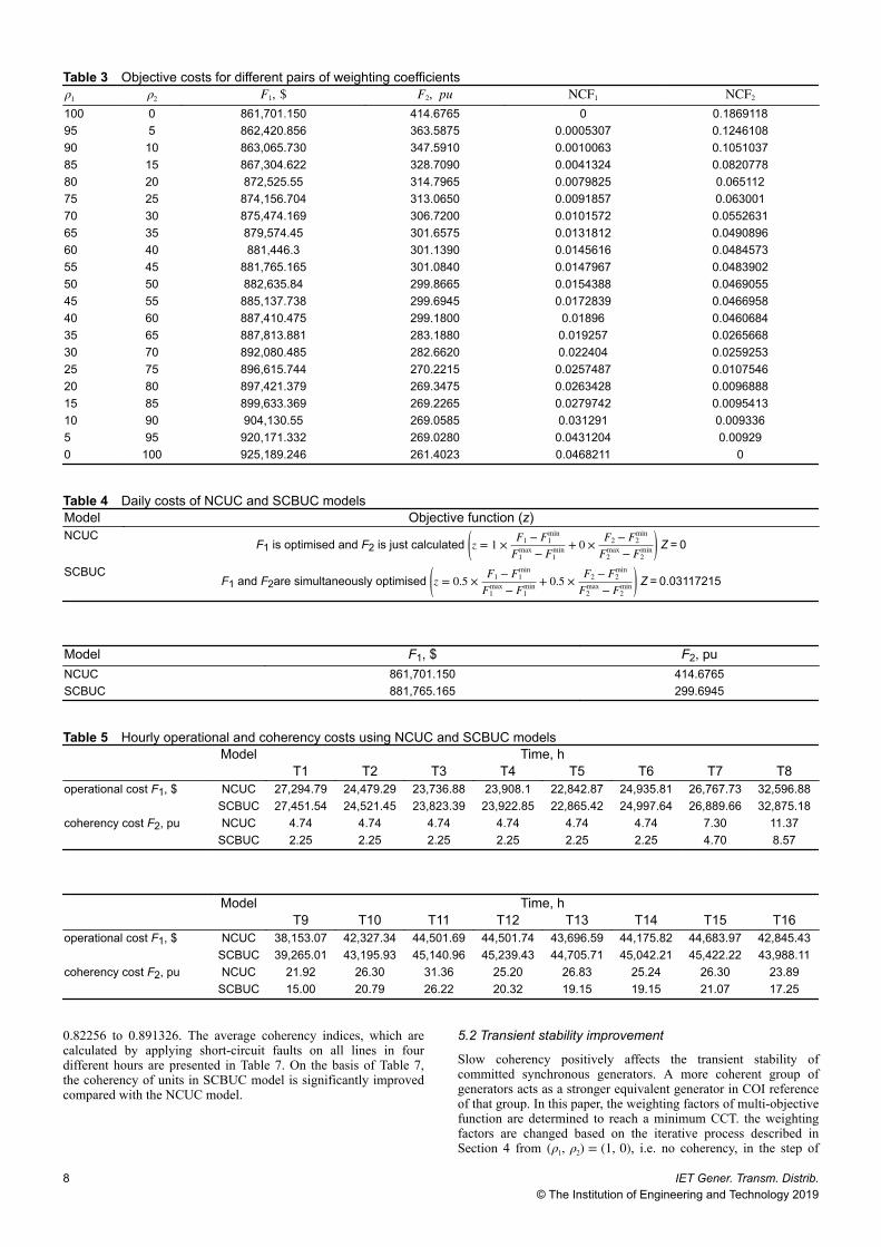
0.82256 to 0.891326. The average coherency indices, which arecalculated by applying short-circuit faults on all lines in fourdifferent hours are presented in Table 7. On the basis of Table 7,the coherency of units in SCBUC model is significantly improvedcompared with the NCUC model.

5.2 Transient stability improvement

Slow coherency positively affects the transient stability ofcommitted synchronous generators. A more coherent group ofgenerators acts as a stronger equivalent generator in COI referenceof that group. In this paper, the weighting factors of multi-objectivefunction are determined to reach a minimum CCT. the weightingfactors are changed based on the iterative process described inSection 4 from (ρ1, ρ2) = (1, 0), i.e. no coherency, in the step of

Table 3 Objective costs for different pairs of weighting coefficientsρ1 ρ2 F1, $ F2, pu NCF1 NCF2

100 0 861,701.150 414.6765 0 0.186911895 5 862,420.856 363.5875 0.0005307 0.124610890 10 863,065.730 347.5910 0.0010063 0.105103785 15 867,304.622 328.7090 0.0041324 0.082077880 20 872,525.55 314.7965 0.0079825 0.06511275 25 874,156.704 313.0650 0.0091857 0.06300170 30 875,474.169 306.7200 0.0101572 0.055263165 35 879,574.45 301.6575 0.0131812 0.049089660 40 881,446.3 301.1390 0.0145616 0.048457355 45 881,765.165 301.0840 0.0147967 0.048390250 50 882,635.84 299.8665 0.0154388 0.046905545 55 885,137.738 299.6945 0.0172839 0.046695840 60 887,410.475 299.1800 0.01896 0.046068435 65 887,813.881 283.1880 0.019257 0.026566830 70 892,080.485 282.6620 0.022404 0.025925325 75 896,615.744 270.2215 0.0257487 0.010754620 80 897,421.379 269.3475 0.0263428 0.009688815 85 899,633.369 269.2265 0.0279742 0.009541310 90 904,130.55 269.0585 0.031291 0.0093365 95 920,171.332 269.0280 0.0431204 0.009290 100 925,189.246 261.4023 0.0468211 0

Table 4 Daily costs of NCUC and SCBUC modelsModel Objective function (z)NCUC

F1 is optimised and F2 is just calculated z = 1 × F1 − F1min

F1max − F1

min + 0 × F2 − F2min

F2max − F2

min Z = 0

SCBUCF1 and F2are simultaneously optimised z = 0.5 × F1 − F1

min

F1max − F1

min + 0.5 × F2 − F2min

F2max − F2

min Z = 0.03117215

 Model F1, $ F2, puNCUC 861,701.150 414.6765SCBUC 881,765.165 299.6945

Table 5 Hourly operational and coherency costs using NCUC and SCBUC modelsModel Time, h

T1 T2 T3 T4 T5 T6 T7 T8operational cost F1, $ NCUC 27,294.79 24,479.29 23,736.88 23,908.1 22,842.87 24,935.81 26,767.73 32,596.88

SCBUC 27,451.54 24,521.45 23,823.39 23,922.85 22,865.42 24,997.64 26,889.66 32,875.18coherency cost F2, pu NCUC 4.74 4.74 4.74 4.74 4.74 4.74 7.30 11.37

SCBUC 2.25 2.25 2.25 2.25 2.25 2.25 4.70 8.57

 Model Time, h

T9 T10 T11 T12 T13 T14 T15 T16operational cost F1, $ NCUC 38,153.07 42,327.34 44,501.69 44,501.74 43,696.59 44,175.82 44,683.97 42,845.43

SCBUC 39,265.01 43,195.93 45,140.96 45,239.43 44,705.71 45,042.21 45,422.22 43,988.11coherency cost F2, pu NCUC 21.92 26.30 31.36 25.20 26.83 25.24 26.30 23.89

SCBUC 15.00 20.79 26.22 20.32 19.15 19.15 21.07 17.25

8 IET Gener. Transm. Distrib.© The Institution of Engineering and Technology 2019

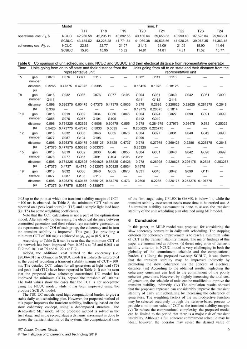
0.05 up to the point at which the transient stability margin of CCT = 100 ms is obtained. In Table 8, the minimum CCT values arereported on a peak load hour (i.e. T12) and a sample light load hour(i.e. T5) for some weighting coefficients.

Note that the CCT calculation is not a part of the optimisationmodel. Alternatively, by decreasing the electrical distance betweencommitted generators and their related representative generator, asthe representative of COI of each group, the coherency and in turnthe transient stability is improved. This goal (i.e. providing aminimum CCT of 100 ms) is achieved at (ρ1, ρ2) = (0.5, 0.5).

According to Table 8, it can be seen that the minimum CCT ofthe network has been improved from 0.052 s at T5 and 0.061 s atT12 to 0.101 s at T5 and 0.122 s at T12.

Indeed, the additional cost related to the coherency (i.e.$20,064.015 as obtained in SCBUC model) is indirectly interpretedas the cost of providing a transient stability margin of CCT = 100 ms. The detailed CCT values for all generators at light load (T5)and peak load (T12) have been reported in Table 9. It can be seenthat the proposed slow coherency constrained UC model hasimproved the minimum CCTs, beyond the threshold of 100 ms.The bold values show the cases that the CCT is not acceptableusing the NCUC model, while it has been improved using theproposed SCBUC model.

The TSC UC models need high computational burden to give astable daily unit scheduling plan. However, the proposed method ofthis paper improves the transient stability, indirectly, based on theslow coherency concept, using a decomposed structure. Thesteady-state MIP model of the proposed method is solved in thefirst stage, and in the second stage a dynamic assessment is done toassess the transient stability of the system. The computational time

of the first stage, using CPLEX in GAMS, is below 1 s, while thetransient stability assessment needs more time to be carried out. A5 s transient stability assessment is done to assess the transientstability of the unit scheduling plan obtained using MIP model.

6 ConclusionIn this paper, an MILP model was proposed for considering theslow coherency constraint in daily unit scheduling. The stoppingcriterion for coherency improvement is to reach a minimum valueof CCT as the transient stability margin. The major findings of thispaper are summarised as follows. (i) direct integration of transientstability criterion in NCUC model is very challenging in both theglobality of the commitment schedule and the computationalburden. (ii) Using the proposed two-step SCBUC, it was shownthat the transient stability may be improved indirectly bypromoting the slow coherency via the concept of electricaldistance. (iii) According to the obtained results, neglecting thecoherency constraint can lead to the commitment of the poorlycoherent generators. However, by slightly increasing the total costof generation, the schedule of units can be modified to improve thetransient stability, indirectly. (iv) The simulation results showedthat the proposed approach can considerably improve the transientstability of daily unit scheduling by increasing the coherency ofgenerators. The weighting factors of the multi-objective functionmay be selected accurately through the iterative-based process toprovide a minimum value of CCT as the transient stability margin.(v) To reduce the computational complexity, the proposed modelcan be limited to the period that there is a major risk of transientinstability. Although a full coherent commitment schedule may beideal, however, the operator may select the desired value of

 Model Time, h

T17 T18 T19 T20 T21 T22 T23 T24operational cost F1, $ NCUC 42,236.58 42,205.11 40,892.55 40,130.64 39,658.33 40,993.40 37,525.04 29,943.91

SCBUC 43,454.62 43,225.28 41,771.54 41,069.38 40,535.56 41,920.25 39,078.35 31,363.45coherency cost F2, pu NCUC 22.83 22.77 21.07 21.13 21.09 21.09 15.90 14.64

SCBUC 15.95 15.95 15.32 14.81 14.81 14.81 11.52 10.77

Table 6 Comparison of unit scheduling using NCUC and SCBUC and their electrical distance from representative generatorTime Units going from on to off state and their distance from the

representative unitUnits going from off to on state and their distance from the

representative unitT5 gen

numberG070 G076 G077 G113 — — G082 G111 G116 — — —

distance,pu

0.3265 0.47375 0.47375 0.3395 — — 0.16425 0.1976 0.18125 — — —

T8 gennumber

G018 G032 G036 G076 G077 G105 G004 G031 G040 G042 G061 G090G113 — — — — — G111 G112 G116 — — —

distance,pu

0.598 0.526375 0.60475 0.47375 0.47375 0.5033 0.278 0.2695 0.228625 0.22625 0.281875 0.26480.339 — — — — — 0.19775 0.20675 0.1814 — — —

T10 gennumber

G018 G019 G032 G034 G036 G046 G004 G024 G027 G090 G091 G099G055 G076 G077 G104 G105 — G112 G040 — — — —

distance,pu

0.598 0.764225 0.52625 0.9008 0.60475 0.555 0.278 0.284575 0.27975 0.26475 0.512 0.253250.5425 0.473775 0.47375 0.5033 0.5035 — 0.256825 0.225775 — — — —

T12 gennumber

G018 G032 G036 G046 G055 G076 G004 G027 G031 G040 G042 G090G077 G087 G104 G105 — — G099 — — — — —

distance,pu

0.598 0.526375 0.60475 0.555125 0.5425 0.4737 0.278 0.27975 0.269425 0.2286 0.226175 0.26480.47375 0.477575 0.50325 0.503375 — — 0.25325 — — — — —

T15 gennumber

G018 G019 G032 G036 G046 G055 G004 G031 G040 G042 G090 G099G076 G077 G087 G091 G104 G105 G111 — — — — —

distance,pu

0.598 0.764225 0.52625 0.604825 0.55525 0.5426 0.278 0.26925 0.228625 0.226175 0.2648 0.2532750.47375 0.4737 0.4775 0.512075 0.50325 0.5034 0.1975 — — — — —

T19 gennumber

G018 G032 G036 G046 G055 G076 G031 G040 G042 G099 G111 —G077 G087 G105 G113 — — — — — — — —

distance,pu

0.598 0.526375 0.60475 0.555125 0.54275 0.473 0.2695 0.2285 0.226175 0.253275 0.197575 —0.47375 0.477575 0.5035 0.338975 — — — — — — — —

IET Gener. Transm. Distrib.© The Institution of Engineering and Technology 2019

9

Fig. 5  Comparison of generators’ speeds with and without considering coherency constraint

Table 7 Comparison of average coherency indices in different hoursGroup number Time, h

SCBUC model average correlation NCUC model average correlationT5

group 1 0.985 0.926group 2 0.956 0.850group 3 0.899 0.768

T8group 1 0.910 0.895group 2 0.930 0.813group 3 0.855 0.732

T12group 1 0.957 0.936group 2 0.932 0.850group 3 0.887 0.730

T8group 1 0.961 0.935group 2 0.942 0.856group 3 0.884 0.822

Table 8 CCT results for different weighting factorsTime, h Minimum CCT, s

(ρ1, ρ2)(1, 0) (0.9, 0.1) (0.7, 0.3) (0.8, 0.2) (0.6, 0.4) (0.5, 0.5)

T5 0.052 0.052 0.068 0.079 0.095 0.101T12 0.061 0.073 0.087 0.909 0.117 0.122

10 IET Gener. Transm. Distrib.© The Institution of Engineering and Technology 2019

coherency by its willingness to pay the additional cost for transientstability improvement. Future works can investigate the effects ofthis improvement on small signal stability of the power system.

7 References[1] Fu, Y., Shahidehpour, M., Li, Z.: ‘Security-constrained unit commitment with

AC constraints’, IEEE Trans. Power Syst., 2005, 20, (3), pp. 1538–1550[2] Castillo, A., Laird, C., Silva-Monroy, C.A., et al.: ‘The unit commitment

problem with AC optimal power flow constraints’, IEEE Trans. Power Syst.,2016, 31, (6), pp. 4853–4866

[3] Zárate-Miñano, R., Van Cutsem, T., Milano, F., et al.: ‘Securing transientstability using time-domain simulations within an optimal power flow’, IEEETrans. Power Syst., 2010, 25, (1), pp. 243–253

[4] Xu, Y., Dong, Z.Y., Meng, K., et al.: ‘A hybrid method for transient stability-constrained optimal power flow computation’, IEEE Trans. Power Syst.,2012, 27, (4), pp. 1769–1777

[5] Sun, Y.-Z., Xinlin, Y., Wang, H.F.: ‘Approach for optimal power flow withtransient stability constraints’, IEE Proc., Gener. Transm. Distrib., 2004, 151,(1), pp. 8–18

[6] Jiang, Q., Huang, Z.: ‘An enhanced numerical discretization method fortransient stability constrained optimal power flow’, IEEE Trans. Power Syst.,2010, 25, (4), pp. 1790–1797

[7] Xu, Y., Dong, Z.Y., Zhang, R., et al.: ‘A decomposition-based practicalapproach to transient stability-constrained unit commitment’, IEEE Trans.Power Syst., 2015, 30, (3), pp. 1455–1464

[8] Jiang, Q., Zhou, B., Zhang, M.: ‘Parallel augment Lagrangian relaxationmethod for transient stability constrained unit commitment’, IEEE Trans.Power Syst., 2013, 28, (2), pp. 1140–1148

[9] Wang, C., Fu, Y.: ‘Fully parallel stochastic security-constrained unitcommitment’, IEEE Trans. Power Syst., 2016, 31, (5), pp. 3561–3571

[10] Ahmadi, H., Ghasemi, H.: ‘Security-constrained unit commitment withlinearized system frequency limit constraints’, IEEE Trans. Power Syst.,2014, 29, (4), pp. 1536–1545

[11] Restrepo, J.F., Galiana, F.D.: ‘Unit commitment with primary frequencyregulation constraints’, IEEE Trans. Power Syst., 2005, 20, (4), pp. 1836–1842

[12] Teng, F., Trovato, V., Strbac, G.: ‘Stochastic scheduling with inertia-dependent fast frequency response requirements’, IEEE Trans. Power Syst.,2016, 31, (2), pp. 1557–1566

[13] Khalil, A.M., Iravani, R.: ‘A dynamic coherency identification method basedon frequency deviation signals’, IEEE Trans. Power Syst., 2016, 31, (3), pp.1779–1787

[14] Wu, D., Lin, C., Perumalla, V., et al.: ‘Impact of grid structure on dynamics ofinterconnected generators’, IEEE Trans. Power Syst., 2014, 29, (5), pp. 2329–2337

[15] Kundur, P., Balu, N.J., Lauby, M.G.: ‘Power system stability and control’, vol.7, (McGraw-Hill, New York, 1994)

[16] Yang, B., Vittal, V., Heydt, G.T.: ‘Slow-coherency-based controlled islanding;a demonstration of the approach on the August 14, 2003 blackout scenario’,IEEE Trans. Power Syst., 2006, 21, (4), pp. 1840–1847

[17] Carrion, M., Arroyo, J.M.: ‘A computationally efficient mixed-integer linearformulation for the thermal unit commitment problem’, IEEE Trans. PowerSyst., 2006, 21, (3), pp. 1371–1378

[18] Ostrowski, J., Anjos, M.F., Vannelli, A.: ‘Tight mixed integer linearprogramming formulations for the unit commitment problem’, IEEE Trans.Power Syst., 2012, 27, (1), pp. 39–46

Table 9 CCT values for different machines assuming (ρ1, ρ2) = (0.5, 0.5)Fault Location CCT

NCUC SCBUCT5 T12 T5 T12

B4 — — — 0.521B10 0.305 0.162 0.421 0.275B12 0.580 0.175 0.566 0.312B18 — 0.162 — —B25 0.342 0.214 0.368 0.256B26 0.421 0.228 0.415 0.274B27 — — — 0.697B31 — — — 1.781B32 — 0.557 — —B36 — 0.356 — —B40 — — — 0.874B42 — — — 1.312B46 — 0.168 — —B49 0.078 0.215 0.11 0.235B54 — 0.42 — 0.42B55 — 0.254 — —B59 — 0.619 — 0.461B61 — 0.415 — 0.354B65 0.083 0.447 0.123 0.306B66 0.09 0.485 0.126 0.324B70 0.052 0.378 0.101 0.914B76 0.081 0.227 — —B77 0.081 0.181 — —B80 0.082 0.121 0.118 0.213B82 — 0.265 0.521 0.465B87 — 0.061 — —B89 0.377 0.061 0.315 0.315B90 — — — 0.974B92 0.074 0.081 0.232 0.526B99 — — — 0.329B100 0.086 0.187 0.25 0.338B104 — 0.726 — —B105 — 0.426 — —B111 — 0.812 1.125 0.725B112 — 1.064 — 0.78B113 0.942 0.699 — 0.491B116 — 0.221 0.161 0.122

IET Gener. Transm. Distrib.© The Institution of Engineering and Technology 2019

11

[19] Zhang, H., Heydt, G.T., Vittal, V., et al.: ‘An improved network model fortransmission expansion planning considering reactive power and networklosses’, IEEE Trans. Power Syst., 2013, 28, (3), pp. 3471–3479

[20] Taylor, J.A., Halpin, S.M.: ‘Approximation of generator coherency based onsynchronization coefficients’. 2007 39th Southeastern Symp. System Theory,Macon, GA, 2007, pp. 47–51

[21] Taylor, J.A., Sayler, K.A., Halpin, S.M.: ‘Approximate prediction of generatordynamic coupling using load flow data’. 2006 38th North American PowerSymp., Carbondale, IL, 2006, pp. 289–294

[22] Marler, R.T., Arora, J.S.: ‘Survey of multi-objective optimization methods forengineering’, Struct. Multidiscip. Optim., 2004, 26, (6), pp. 369–395

[23] Available at https://github.com/anyacastillo/ucacopf/blob/master/118_ucacopf.dat. Accessed: 15 January 2018

[24] Available at http://www.kios.ucy.ac.cy/testsystems/index.php/dynamic-ieee-test-systems/ieee-118-bus-modified-test-system. Accessed: 15 January 2018

[25] I. CPLEX: ‘ILOG CPLEX homepage 2009’. Available at https://www.ibm.com/products/ilog-cplex-optimization-studio, 2009. Accessed: 15January 2018

[26] Anderson, P.M., Anderson, P.: ‘Power system protection’, vol. 1307,(McGraw-Hill, New York, 1999)

12 IET Gener. Transm. Distrib.© The Institution of Engineering and Technology 2019