RESEARCH ARTICLE10.1002/2016WR018716

Transferring measured discharge time series: Large-scalecomparison of Top-kriging to geomorphology-based inversemodelingA. de Lavenne1,2, J. O. Skøien3, C. Cudennec4,5, F. Curie1, and F. Moatar1

1Universit�e Francois Rabelais - Tours, EA 6293, G�eo-Hydrosystemes Continentaux, Facult�e des Sciences et Techniques,Tours, France, 2Now at Irstea, Hydrosystems and Bioprocesses Research Unit, Antony, France, 3European Commission,Joint Research Centre, Institute for Environment and Sustainability, Climate Risk Management Unit, Ispra, Italy,4AGROCAMPUS OUEST, UMR1069, Sol Agro et hydrosysteme Spatialisation, Rennes, France, 5INRA, UMR1069, Sol Agro ethydrosysteme Spatialisation, Rennes, France

Abstract Few methods directly transfer streamflow measurements for continuous prediction of unga-uged catchments. Top-kriging has been used mainly to predict the statistical properties of runoff but hasbeen shown to outperform traditional regionalization approaches of rainfall-runoff models. We applied theTop-kriging approach across the Loire River basin and compared predictions to a geomorphology-basedapproach. Whereas Top-kriging uses spatial correlation, the other approach has the advantage of beingmore physically based by using a well-known geomorphology-based hydrological model (WFIUH) and itsinversion. Both approaches require an equal degree of calibration and provide similar performances. Wealso demonstrate that the Ghosh distance, which considers the nested nature of catchments, can be usedefficiently to calculate weights and to identify the suitability of gauged catchments for use as donor catch-ments. This result is particularly relevant for catchments with Strahler orders above five, i.e., where donorcatchments are more strongly nested.

1. Introduction

The previous IAHS decade on ‘‘Predictions in Ungauged Basins’’ (PUB) resulted in a large amount of litera-ture on the issue of ungauged catchments [Sivapalan et al., 2003; Hrachowitz et al., 2013; Bl€oschl et al., 2013].Regionalization techniques are a deeply studied subset of methods.

Different definitions of ‘‘regionalization’’ exist; in runoff hydrology, the term generally refers to methods forinterpolating hydrological information to ungauged catchments [He et al., 2011]. Most often this is achievedby assessing hydrological similarities or developing statistical relations between the desired variables,parameters and easily observable catchment characteristics.

Among the regionalization approaches for predicting continuous streamflow, few methods transfer directobservations of the variable of interest. Most are based on rainfall-runoff models that are applied in bothgauged and ungauged locations, and regionalization techniques are then used to interpolate the calibratedmodel parameters [see for instance Vandewiele et al., 1991; Merz and Bl€oschl, 2004; Oudin et al., 2008, 2010].One limitation of the approach is that, in addition to the uncertainty in the estimated parameters, issuesinherent in the model itself are also transferred (simplifying hypotheses, issues related to parameters’ identi-fication, rainfall uncertainty, etc.).

An alternative approach which avoids these problems, and which can be applied when the causal rainfall-runoff relation is not needed, is to regionalize streamflow properties directly. The greatest limitation in mostcases is the uncertainty in magnitude and spatial distribution of rainfall for both the gauged and ungaugedcatchments. Runoff observations also naturally integrate human influence, such as dams or water with-drawals for irrigation, which is challenging to model consistently.

Several observation-based approaches found in the literature rely on geostatistical techniques to spatiallyinterpolate variables measured in the stream network [Skøien et al., 2006; Isaak et al., 2014; M€uller andThompson, 2015; Farmer, 2016]. Topological kriging (or Top-kriging) of a variety of variables was recently

Key Points:� The geomorphological inversion

approach and Top-kriging are equallyefficient for continuous streamflowsimulation� Small upstream catchments have

higher uncertainties than largercatchments for both methods� A rescaled Ghosh distance provides

the best weighting of donorcatchments for geomorphologicalinversion

Supporting Information:� Supporting Information S1

Correspondence to:A. de Lavenne,alban.de-lavenne@irstea.fr

Citation:de Lavenne, A., J. O. Skøien,C. Cudennec, F. Curie, and F. Moatar(2016), Transferring measureddischarge time series: Large-scalecomparison of Top-kriging togeomorphology-based inversemodeling, Water Resour. Res., 52,doi:10.1002/2016WR018716.

Received 5 MAR 2016

Accepted 15 JUN 2016

Accepted article online 17 JUN 2016

VC 2016. American Geophysical Union.

All Rights Reserved.

DE LAVENNE ET AL. TRANSFERRING MEASURED DISCHARGE TIME SERIES 1

Water Resources Research

PUBLICATIONS

compared to several other methods. Archfield et al. [2013] demonstrated that Top-kriging substantially out-performed a regression approach (with observable catchment descriptors) and canonical kriging (physio-graphical space-based interpolation) in estimating flood quantiles of 61 catchments in the southeasternUnited States. Laaha et al. [2014] also compared Top-kriging with the traditional regression approach for300 Austrian catchments to estimate low flow quantiles. They showed that Top-kriging generally performedbetter, or at locations without upstream observations, as well as the regression approach. Recently, M€ullerand Thompson [2015] also evaluated their own kriging strategy, called TopREML, in a comparison with Top-kriging. They demonstrated similar performances for mean streamflow and runoff frequency but better pre-dictions of model uncertainties.

Kriging has sometimes also been used to interpolate runoff time series. Farmer [2016] used ordinary kriging at adaily time step, whereas Skøien and Bl€oschl [2007] extended their topological kriging technique for this purposeat an hourly time step. Viglione et al. [2013] demonstrated that this spatiotemporal Top-kriging also outperformsregionalized rainfall-runoff models for the daily streamflow prediction of 213 Austrian catchments.

Patil and Stieglitz [2012] also directly transferred daily streamflow time series in the U.S. and weighted donorcatchments using inverse-distance weighting (IDW) between stream gauges. They used the prediction per-formance to identify regions where nearby catchments tend to have similar streamflow patterns and dem-onstrated that spatial proximity between donor and receiver catchments alone cannot fully explain theprediction performance at a given location.

An alternative method to transfer hydrograph measures was developed by Andr�eassian et al. [2012]. They devel-oped simple equations (from one to three parameters) that facilitate the transfer of daily and hourly streamflowtime series. They averaged predictions from seven donor catchments and demonstrated that this approach,which they called ‘‘nature’s own hydrological model,’’ was as efficient as a calibrated rainfall-runoff model.

Originally formulated by Cudennec [2000] and then applied to different contexts [Boudhraa, 2007; Boudhraa et al.,2006, 2009; de Lavenne et al., 2015], a geomorphology-based inverse/direct modeling approach transfers anobserved hydrograph of a gauged catchment to ungauged catchments, either nested, neighboring or similar.This work is based on estimating net rainfall from runoff discharge measurements, which facilitates direct transfer.

Following the idea that transferring direct measurements is an attractive alternative for several practicalPUB issues, the aim of this study was twofold: (1) to explore the geomorphology-based approach for a largenumber of catchments, beyond the methodological validation for a small number of gauged catchmentsthat had already been performed; (2) to compare Top-kriging and the geomorphology-based approachesfor predicting continuous streamflow. We facilitated this comparison by using a similar calibration approachand distance functions for all catchments. The analyses were performed on a comprehensive dataset forthe Loire River basin, the largest French basin (117,500 km2), which provides a range of cascading and paral-lel gauged subbasins with high geographic heterogeneity.

2. Methods

Both approaches were analyzed with the statistical environment R [R Core Team, 2015]. Top-kriging was pre-viously implemented in the rtop package [Skøien et al., 2014] and was extended for this study to also per-form topological kriging of time series.

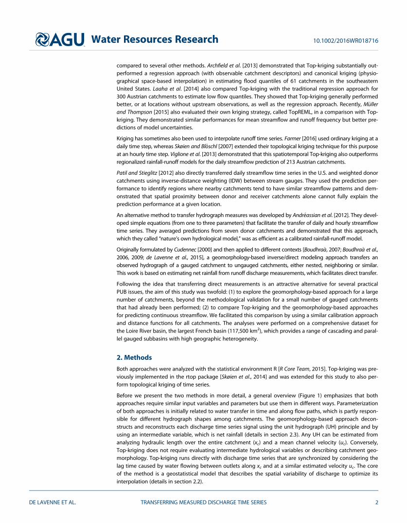
Before we present the two methods in more detail, a general overview (Figure 1) emphasizes that bothapproaches require similar input variables and parameters but use them in different ways. Parameterizationof both approaches is initially related to water transfer in time and along flow paths, which is partly respon-sible for different hydrograph shapes among catchments. The geomorphology-based approach decon-structs and reconstructs each discharge time series signal using the unit hydrograph (UH) principle and byusing an intermediate variable, which is net rainfall (details in section 2.3). Any UH can be estimated fromanalyzing hydraulic length over the entire catchment (xc) and a mean channel velocity (uc). Conversely,Top-kriging does not require evaluating intermediate hydrological variables or describing catchment geo-morphology. Top-kriging runs directly with discharge time series that are synchronized by considering thelag time caused by water flowing between outlets along xc and at a similar estimated velocity uc. The coreof the method is a geostatistical model that describes the spatial variability of discharge to optimize itsinterpolation (details in section 2.2).

Water Resources Research 10.1002/2016WR018716

DE LAVENNE ET AL. TRANSFERRING MEASURED DISCHARGE TIME SERIES 2

2.1. Velocity Estimation and Rising TimesBoth approaches require estimating only one parameter: streamflow velocity uc. We regionalized thisparameter and used it identically in both approaches to facilitate their comparison. Based on the work of deLavenne [2013], we applied an algorithm to detect and extract rising times TRi of catchment i from itsobserved runoff. The algorithm analyzes runoff time series to find noticeable rises.

This analysis is based on two main criteria: (1) slope of the rise: relative change in runoff per time step mustexceed 0.75% h21 at the beginning of the rising limb and 0.1% h21 during the rising limb; (2) surface runoffvolume and intensity: the area under the runoff curve during the rising limb, and greater than the first run-off value of the event, is used to approximate the amount of flowing water. Its volume must be greater than0.005 mm and its intensity more than 0.004 mm h21. Because the hydrograph can have a complex rise (i.e.,with small fluctuations), a rising limb is identified when discharge increases during a period of six timesteps. The rising limb is considered to end when discharge decreases for more than 8 h.

Streamflow velocity is then estimated from the mean hydraulic length and the rising times TRi.

uic5

xc

TRi(1)

The multiple estimates of streamflow velocity enabled a regional relation between rising times and stream-flow velocity to be determined (Figure 2):

uc5a � xcb (2)

where a54:3831024 and b 5 0.69.

2.2. Spatiotemporal Kriging Method2.2.1. Top-KrigingTop-kriging can be seen as a combination of two processes inside a geostatistical framework that controlsthe streamflow. The first is continuous in space and corresponds to runoff generation, which mainlydepends on rainfall, evapotranspiration and soil characteristics. This variable is conceptualized by a point

Figure 1. Conceptual comparison and input variables used by the two approaches for transferring discharge time series.

Water Resources Research 10.1002/2016WR018716

DE LAVENNE ET AL. TRANSFERRING MEASURED DISCHARGE TIME SERIES 3

process that is assumed to exist overthe entire catchment. This variability ina geostatistical framework can bedescribed by Euclidean distances, andits spatial statistical characteristics arerepresented by a variogram [Skøienet al., 2006]. Generated runoff(zðA1Þ; zðA2Þ,. . ., z(An)) cannot beobserved continuously in space but isobserved as a spatial aggregate atstream gauges where

zðAiÞ51jAij

ðAi

zðxÞdx (3)

and Ai is the spatial support of z(Ai).For streamflow variables, Ai is theupstream area of a catchment thatdrains into a river location xi, and |Ai| isits surface area.

The second variable is the flow routingin the stream network. It results fromthe accumulation and aggregation ofrunoff along the network, such asthose in nested catchments. This vari-

able is defined by one point in the stream network, which is the outlet of the catchment. Contrary to the firstvariable, it cannot be represented by Euclidean distances but needs a method that reflects the tree structureof the stream network.

Top-kriging aims to integrate these two aspects, which define the hydrological response of one catchment, tointerpolate streamflow-related information between catchments. Skøien and Bl€oschl [2007] interpolated runofftime series by conceptualizing the aggregate at the outlet as the convolution of the runoff generated within thecatchment during the time needed by the generated runoff to reach the outlet. In this study we assume that,after calibration, an integrated spatial variogram is numerically similar to an integrated space-time variogram,similar to that developed by [Skøien et al., 2006]. We applied Top-kriging to runoff time series by assuming thatrunoff is only spatially correlated with time series [Kyriakidis and Journel, 1999]. For each time step tx, specificrunoff qðxi; txÞ of an ungauged target catchment defined by location xi is estimated from observed specific run-off qðxj; taÞ at the same time step ta5tx of neighboring gauged catchments located at xj as

qðxi ; txÞ5Xn

j51

kjqðxj; taÞ (4)

From the hypothesis of stationarity and the randomness of runoff generation processes, optimal weights kj

can be found by solving the kriging system:

Xn

k51

kkcjk2kjr2j 1l5cij j51; . . . ; n

Xn

j51

kj51

(5)

where the gamma values cij and cjk are the expected semivariances between the ungauged catchment iand the neighbors j used for estimation, and between two neighbors j and k, respectively. The variable l isthe Lagrange parameter, and r2

i represents the measurement error or uncertainty in measurement i.

Because measurements are related to a nonzero support A, the semivariance cij between two measure-ments with catchment areas Ai and Aj must be obtained from regularization [Cressie, 1993]. Also, because

Figure 2. Comparison of velocity estimated from regression and velocityestimated from rising time.

Water Resources Research 10.1002/2016WR018716

DE LAVENNE ET AL. TRANSFERRING MEASURED DISCHARGE TIME SERIES 4

the size of the drained area increases from upstream to downstream, the transfer of information from oneoutlet to another implies a change of support. For this reason, the variogram model must be regularized foreach combination of catchment areas. This accounts for the different scales and nested nature of the catch-ments. Assuming the existence of a point semivariogram cp, the expected semivariance cij between twoobservations of catchment areas Ai and Aj is

cij50:5 � VarðzðAiÞ2zðAjÞÞ

51

AiAj

ðAi

ðAi

cpðjx12x2jÞdx1dx220:5 � 1A2

i

ðAi

ðAj

cpðjx12x2jÞdx1dx211

A2j

ðAj

ðAj

cpðjx12x2jÞdx1dx2

" #(6)

where x1 and x2 are position vectors within each catchment used for integration. The first part of equation(6) finds the mean of the point variogram between the two catchments. The second part generates asmoothing effect by subtracting the mean of the point variogram within the two catchments. This formula-tion considers the nested nature of two catchments: their semivariance will decrease as the overlap of theirsupport increases. To facilitate the calculation, the integrals in equation (6) are replaced by sums, and catch-ment areas are discretized by a regular grid (Figure 3).

To simplify the calculation, Gottschalk [1993] and Gottschalk et al. [2011] suggested applying the covariancemodel to the mean distance between areas, d�ij , instead of calculating the covariance for each distance andthen calculating the mean.

d�ij 51

jAi jjAj j

ðAi

ðAj

ðjxi2xjjÞdxi dxj (7)

We henceforth refer to this distance as the Ghosh [1951] distance. The regularized semivariance betweentwo areas then simply becomes

c�ij 5cpðd�ij Þ20:5 � ðcpðd�ii Þ1cpðd�jj ÞÞ (8)

where d�ii represents the mean distances within Ai.2.2.2. Top-Kriging of Time SeriesSkøien and Bl€oschl [2007] extended the Top-kriging approach to address runoff time series. Based on theanalysis of Skøien and Bl€oschl [2006], which described catchment behavior as a space-time filter, Skøien andBl€oschl [2007] developed spatiotemporal Top-kriging to consider space and time correlation of runoff timeseries along the stream network.

Figure 3. Discretization of two catchment areas A1 and A2 using points x1 and x2 to evaluate distances [from Skøien et al., 2006].

Water Resources Research 10.1002/2016WR018716

DE LAVENNE ET AL. TRANSFERRING MEASURED DISCHARGE TIME SERIES 5

This approach considers routing within a catchment but not between catchments. Consequently, Skøienand Bl€oschl [2007] developed a simple routing model that considers the time shift caused by water flowingfrom an upstream to a downstream catchment.

Skøien and Bl€oschl [2007] demonstrated that this routing, combined with spatial kriging, yielded predictionsbetter than those of spatiotemporal kriging. On this basis, we implemented spatial kriging, as previouslydescribed, but supplemented it with a simple routing routine. It should be noted that this assumption is anappropriate choice for a regular time series, but that full spatiotemporal kriging is necessary when timeseries are irregular, if the degree of intermittency in the time series is high, or if the intention of the interpo-lation is to increase the temporal resolution of the time series.

The routing routine consists of estimating the time shift that may be observed between catchments, whichis due to advection and hydrological dispersion [Rinaldo et al., 1991]. Thus, we estimate qðxi; txÞ from theneighboring observations qðxj; t�aÞ at time steps t�a5ta1t0a instead of ta in equation (4), where t0a reflects thetime shift or difference in response time of the two catchments.

There are several ways to estimate this time shift. One option is to calculate the time shift t0ija betweencatchments i and j, as the difference between regionalized rising times for the studied region (see section2.1 above for more details). The time shift is then estimated from the difference between their estimated ris-ing times TLi and TLj:

t0ija5TLj2TLi (9)

where TLi and TLj are respectively the rising times of catchments i and j. It is important to note that t0ija canbe negative.

To estimate the effect of the routing, we also performed an alternative variant of Top-kriging in which thetime shift was set to zero.

t0ija50 (10)

Both rising time estimates are found from equation (11).

TLi5xc

uc(11)

where xc is the mean hydraulic length, and uc is the streamflow velocity estimated by equation (2).

We consider TLi and TLj an approximation of catchment response time, an approximation of the time need-ed by rainfall to trigger the main streamflow response of catchments i and j. If we assume spatially homoge-neous rainfall over the catchments, t0ija is thus equivalent to the time separating their peak flows. Thisapproach may be more realistic than focusing only on the time needed by water to flow from one outlet toanother within the river network (which then requires distinguishing nested/nonnested catchments). Adownstream catchment does not receive water only from upstream river flow but also from its own hill-slopes and other tributaries. Considering only streamflow travel time may underestimate the time shift sep-arating two catchments. Conversely, TLi and TLj are influenced by travel time through hillslopes; so, theirdifference consequently also considers hillslope travel time (the effect depends on the catchment size; seefor instance D’Odorico and Rigon [2003]), whereas the opposite is the case for higher Strahler orders.2.2.3. Choice of Variogram ModelWe chose the nonstationary version of the exponential variogram model because Skøien et al. [2006] dem-onstrated that it works well for interpolating hydrological data and because it has few parameters.

2.3. Transferring Hydrograph by the Width Function Inversion MethodThis method was originally formulated by Cudennec [2000]. It was applied in a semiarid context in Tunisia[Boudhraa, 2007; Boudhraa et al., 2006, 2009] and more recently in oceanic temperate France [de Lavenne,2013; de Lavenne and Cudennec, 2015; de Lavenne et al., 2015].2.3.1. A Geomorphology-Based ModelAs discussed by Robinson et al. [1995] and similar to Top-kriging, this approach distinguishes runoff generationover hillslopes (production function) from flow routing in the stream network (transfer function). The approachfocuses only on the transfer function, which is built from a morphometric description of the flow path within

Water Resources Research 10.1002/2016WR018716

DE LAVENNE ET AL. TRANSFERRING MEASURED DISCHARGE TIME SERIES 6

the river network [Cudennec et al., 2004; Cudennec and Fouad, 2006; Cudennec, 2007; Aouissi et al., 2013]. Thehydraulic length xc, defined as the distances to the outlet from any point within the river network, is estimatedfrom a digital elevation model (DEM) of the catchment and is described as a probability density function(pdf(xc)) of distances. Assuming a linear transfer function throughout the river network [Naden, 1992; Beven andWood, 1993; Bl€oschl and Sivapalan, 1995; Robinson et al., 1995; Yang et al., 2002; Giannoni et al., 2003b, 2003a;Rodriguez et al., 2005], an estimate of a mean channel flow velocity (uc) provides the pdf of water travel time tthrough the river network. This pdf is a transfer function and can be referred to as the Unit Hydrograph (UH(t)).This geomorphology-based UH is also usually called the WFIUH (Width Function Instantaneous Unit Hydro-graph) in the literature. To facilitate the comparison with Top-kriging, we used the same approach to estimatechannel flow velocity and the regression described by equation (2).

Assessing UH(t) allows estimation of discharge at the outlet Q (m3 s21) (Step 1, Figure 4) using the followingconvolution:

QðtÞ5S �ðt

0Rnðt2sÞ � UHðsÞ � ds (12)

where t (s) is time, S (m2) is the catchment’s surface area, Rn (m) is net rainfall, and s is a temporal integra-tion variable.2.3.2. Deconvolution and Transfer of the HydrographIn the original application, the hydrograph of the closest gauged catchment is transferred onto an unga-uged catchment using net rainfall as an intermediate variable. Net rainfall Rn is defined as the depth of run-off provided by a catchment’s hillslope into its river network; thus, it is a theoretical concept that existsindependent of rainfall and as long as there is water in the stream. It is estimated from the gauged catch-ment and transferred onto an ungauged catchment. The approach assumes that for a pair of nested orneighboring catchments, the net rainfall of the gauged catchment (donor catchment) can represent the netrainfall of the ungauged one (receiver catchment). This assumption comes from the idea that net rainfall ismore independent of catchment size than the hydrograph itself, and that the shape of the hydrograph isinfluenced by the size and geometry of the catchment. In other words, assessing the net rainfall time seriessolves the scaling issue underlying the transfer of hydrographs.

The hydrograph measured at the outlet of one gauged catchment is used to estimate its net rainfall through adeconvolution of the signal. This is achieved by inverting the gauged catchment’s geomorphology-based transferfunction (Step 2, Figure 4). In this manner, the net rainfall time series is estimated from the discharge time series.Step 3 of the approach (Figure 4) is to transfer this net rainfall onto an ungauged catchment and to perform a con-volution with the ungauged catchment’s transfer function. This is achieved using equation (12), and the resultingtime series is the predicted hydrograph. It is important to note that because the approach is based only on thecatchment’s transfer function, it does not need to include a production function. This would involve a more com-plex modeling approach to describe the highly nonlinear hillslope behaviors.

Figure 4. Principle of direct transfer of a hydrograph [from de Lavenne and Cudennec, 2015].

Water Resources Research 10.1002/2016WR018716

DE LAVENNE ET AL. TRANSFERRING MEASURED DISCHARGE TIME SERIES 7

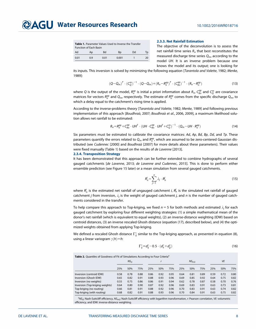
2.3.3. Net Rainfall EstimationThe objective of the deconvolution is to assess thenet rainfall time series Rn that best reconstitutes themeasured discharge time series Qm, according to themodel UH. It is an inverse problem because oneknows the model and its output; one is looking for

its inputs. This inversion is solved by minimizing the following equation [Tarantola and Valette, 1982; Menke,1989]:

ðQ2QmÞT � ðCmQ Þ

21 � ðQ2QmÞ1ðRn2Rapn Þ

T � ðCapRnÞ

21 � ðRn2Rapn Þ (13)

where Q is the output of the model, Rapn is initial a priori information about Rn, Cap

Rn and CmQ are covariance

matrices for vectors Rapn and Qm, respectively. The estimate of Rap

n comes from the specific discharge Qm, towhich a delay equal to the catchment’s rising time is applied.

According to the inverse-problems theory [Tarantola and Valette, 1982; Menke, 1989] and following previousimplementation of this approach [Boudhraa, 2007; Boudhraa et al., 2006, 2009], a maximum likelihood solu-tion allows net rainfall to be estimated:

Rn5Rapn 1Cap

Rn � UHT � ðUH � CapRn � UHT 1Cm

Q Þ21 � ðQm2UH � Rap

n Þ (14)

Six parameters must be estimated to calibrate the covariance matrices: Ad, Ap, Bd, Bp, Dd, and Tp. Theseparameters quantify the errors related to Qm and Rap

n , which are assumed to be zero-centered Gaussian dis-tributed (see Cudennec [2000] and Boudhraa [2007] for more details about these parameters). Their valueswere fixed manually (Table 1) based on the results of de Lavenne [2013].2.3.4. Transposition StrategyIt has been demonstrated that this approach can be further extended to combine hydrographs of severalgauged catchments [de Lavenne, 2013; de Lavenne and Cudennec, 2015]. This is done to perform eitherensemble prediction (see Figure 15 later) or a mean simulation from several gauged catchments.

Rin5Xn

j51

kj � Rjn (15)

where Rin is the estimated net rainfall of ungauged catchment i, Rj

n is the simulated net rainfall of gaugedcatchment j from inversion, kj is the weight of gauged catchment j, and n is the number of gauged catch-ments considered in the transfer.

To help compare this approach to Top-kriging, we fixed n 5 5 for both methods and estimated kj for eachgauged catchment by exploring four different weighting strategies: (1) a simple mathematical mean of thedonor’s net rainfall (which is equivalent to equal weights), (2) an inverse-distance weighting (IDW) based oncentroid distances, (3) an inverse rescaled Ghosh distance (equation (17), described below), and (4) the opti-mized weights obtained from applying Top-kriging.

We defined a rescaled Ghosh distance C�ij similar to the Top-kriging approach, as presented in equation (8),using a linear variogram cðhÞ5h:

C�ij5d�ij 20:5 � ðd�ii 1d�jj Þ (16)

Table 1. Parameter Values Used to Inverse the TransferFunction of Each Basin

Ad Ap Bd Bp Dd Tp

0.01 0.9 0.01 0.001 1 20

Table 2. Quantiles of Goodness of Fit of Simulations According to Four Criteriaa

NSQ r NSlnQ VE

25% 50% 75% 25% 50% 75% 25% 50% 75% 25% 50% 75%

Inversion (centroid IDW) 0.58 0.78 0.88 0.86 0.92 0.95 0.64 0.81 0.89 0.59 0.72 0.80Inversion (Ghosh IDW) 0.65 0.82 0.91 0.88 0.93 0.96 0.69 0.85 0.92 0.64 0.75 0.82Inversion (no weights) 0.55 0.75 0.86 0.86 0.91 0.94 0.62 0.78 0.87 0.58 0.70 0.76Inversion (Top-kriging weights) 0.64 0.80 0.90 0.87 0.92 0.96 0.69 0.83 0.91 0.63 0.73 0.81Top-kriging (no routing) 0.66 0.81 0.91 0.88 0.92 0.96 0.70 0.83 0.91 0.63 0.74 0.82Top-kriging (with routing) 0.68 0.82 0.91 0.88 0.93 0.96 0.70 0.84 0.91 0.63 0.75 0.82

aNSQ: Nash-Suttcliff efficiency, NSlnQ: Nash-Suttcliff efficiency with logarithm transformation, r: Pearson correlation, VE: volumetricefficiency, and IDW: inverse-distance weighting.

Water Resources Research 10.1002/2016WR018716

DE LAVENNE ET AL. TRANSFERRING MEASURED DISCHARGE TIME SERIES 8

This aims to improve the calculation of distance between hydrological variables with two-dimensional sup-ports (catchment areas) [Ghosh, 1951; Gottschalk, 1993; Gottschalk et al., 2011]. As an approximation of theTop-kriging approach, we applied an inverse function to this rescaled Ghosh distance to estimate theweights of the donor catchments:

kij51C�ij� 1Xn

k51

ð1=C�kjÞ

Xn

k51

kkj51

(17)

where kij is the weight of gauged catchment i used to estimate the net rainfall of ungauged catchment j,and n is the number of gauged catchments considered in the transfer. The second equation in the set ofequations (17) allows kij to vary between 0 and 1, and to sum up to 1. In addition, as a hybrid model, weextracted the weights of donor catchments estimated by Top-kriging and applied them when transferringnet rainfall.

As in our application of Top-kriging, we constrained the geographic extent in which gauged catchmentswere selected. Centroids of gauged catchments had to be located within a 50 km radius of the centroidof the ungauged catchment. The closest catchments were chosen when more than n 5 5 catchmentswere located within this radius. We used the centroids’ geographic distance for weighting approaches(1) and (2), and the rescaled Ghosh distance for weighting approaches (3) and (4). When no catchmentcentroids existed within this radius, the catchment centroid with the shortest rescaled Ghosh distancewas used.

3. Application

3.1. Cross ValidationTo examine the relative performances of models more quantitatively, we performed leave-one-out cross-validation. After withholding the streamflow time series of a particular gauge, we predicted the time seriesfor that location, and then compared the prediction to the streamflow observations. This procedure wasrepeated for all gauges and emulated prediction at sites without streamflow observations.

3.2. Efficiency AssessmentWe evaluated the goodness of fit of predictions using four criteria: (1) NSQ, the Nash-Sutcliffe criterion [Nashand Sutcliffe, 1970], which emphasizes errors on high flows; (2) NSlnQ, the Nash-Sutcliffe criterion performedon log-transformed discharges, which emphasizes errors on low flows; (3) r Pearson correlation, which isused to evaluate timing correlation; and (4) VE, the volumetric efficiency developed by Criss and Winston[2008] as an alternative to the Nash-Sutcliffe criterion, which emphasizes the bias on water volume. Theoptimal value of all criteria is equal to 1. The Nash-Sutcliffe criterion has no lower bound, whereas r and VEhave lower bounds equal to 21 and 0, respectively.

These criteria were calculated for all available runoff data, whose duration varied by catchment, asdescribed in section 3.4.

3.3. Morphometric DescriptionTo extract catchment boundaries and to analyze the flow path length required to build the UH (section2.3), we used GRASS 7.0 supplemented by the toolkit of Jasiewicz and Metz [2011]. The hydraulic lengthxi

c of catchment i is estimated over its entire area from a DEM at 25 m resolution. The D8 algorithm wasused to model drainage, and a predefined river network provided by the Sandre/BD CARTHAGE databasewas burned into the DEM using an algorithm based on the inverse distance to the network [Nagel et al.,2011].

3.4. Studied Catchments and DataBoth modeling approaches were applied to the ensemble of all Loire catchments. We chose the mostdownstream outlet, near the city of Mont-Jean-sur-Loire, which drains a surface of about 110,000 km2 and is

Water Resources Research 10.1002/2016WR018716

DE LAVENNE ET AL. TRANSFERRING MEASURED DISCHARGE TIME SERIES 9

not influenced by tides. The catchment has high climatic, geological and hydrological variability. The catch-ment also has a varied climate (oceanic and continental) and lithology.

Three main regions are usually distinguished according to their lithology (Figure 5). The first is a mountain-ous region with a mean elevation of 800 m. It is defined mostly by granite and basalt bedrock. Catchmentsat higher altitudes have a nival influence. Its specific discharges are generally higher than those of the otherregions because of more rainfall (from 500 to >1250 mm/yr) and its lithology, which favors surface runoff.The second region is located on sedimentary rocks and has contrasting hydrological behavior, especiallydue to a large aquifer connected to the river system. Its annual rainfall is lower, averaging 690 mm/yr. Thethird region is composed of granite and basalt and receives an average of 750 mm of rainfall per year.

For 87% of 184 stations analyzed by Sauquet et al. [2008] in the Loire catchment, pluvial river flow regimesdominated. In the mountainous region, only 12% of stations have a transition (pluvio-nival) regime, in whichseasonal variation in streamflow is affected as much by precipitation timing as by air temperature and topo-graphic influences (on snowpack formation and snowmelt timing). Typically, high flows are observed inspring. One percent of stations in the southern part of the Loire catchment are representative of Mediterra-nean river flow regimes, with low flow in summer and high flow in November. The snowmelt-fed regime isnot observed in the Loire catchment. Some stations are influenced by one or more reservoirs which arelocated in the mountainous region: 10% are influenced throughout the year and 8% only during low flow.The two largest dams (totaling 350 Mm3) are Naussac (low flow moderation) and Villerest (low flow modera-tion and flood control). Other, smaller dams (totaling 200 Mm3) are used to generate hydropower.

Discharge measurements were extracted from the French Hydro Database (www.hydro.eaufrance.fr) at vari-able time steps and were converted into hourly time steps. The studied period extended from September2000 to September 2013. Since not all stations in the database had all 13 hydrological years of data, 3 yearsof runoff data was established as a minimum requirement for study (boxplot Figure 5). A total of 389

Figure 5. Specific annual discharge of the Loire catchments (Banque hydro database) with annual precipitation and potential evapotranspiration (PET) from the SAFRAN database(M�et�eo-France). Statistics come from the 2000–2012 time period.

Water Resources Research 10.1002/2016WR018716

DE LAVENNE ET AL. TRANSFERRING MEASURED DISCHARGE TIME SERIES 10

catchments were selected for this study. Mean gauge density is 3.6 gauges per 1000 km2 in the entire studyarea (4.5, 2.6, and 4.6 gauges per 1000 km2 in zones 1, 2, and 3, respectively).

4. Results

4.1. Statistical DistributionGoodness of fit of streamflow predicted for the entire dataset using the geomorphological approach variedby weighting strategy (Figure 6). The worst predictions were obtained when using the simple mathematicalmean of the donor catchments (strategy 1). Predictions improved when using IDW based on centroid dis-tances. The best predictions were obtained from the inverse rescaled Ghosh distance weighting.

This demonstrates that introducing more sophisticated weighting strategies improves the skill of the trans-fer approach. This result differs from Andr�eassian et al. [2012] and de Lavenne [2013], who found the simplemathematical mean as the best approach among those tested. This difference in results could be explainedby the present study’s larger dataset, which yielded a stronger statistical significance. In particular, thisimprovement is more obvious when dealing with larger catchments (see section 4.3).

Retrieving Top-kriging weights and applying the weights in the geomorphological approach did notimprove the goodness of fit, and even produced slightly worse performances. However, the differenceswere quite small and not significant. Consequently, it does not seem worth the effort to apply the hybridapproach rather than the inverse rescaled Ghosh distance approach. A different choice of variogram, how-ever, could potentially influence this. A scatterplot of the two weighting strategies (Figure 7) indicated thatthe values of the weights followed a similar trend. However, Top-kriging tended to smooth the weightsamong donor catchments, whereas the inverse function yielded more contrasting weights (more low andhigh values). In this way, Top-kriging tends to combine the information of all donor catchments, whereasinverse rescaled Ghosh distance weighting attributes most of the weight to the nearest catchments.

Comparison of goodness-of-fit criteria showed that the weighting strategy seemed to have slightly moreinfluence on high flows (estimated by NSQ) than low flows (estimated by NSlnQ) and on volume efficiency.Conversely, timing correlation (estimated by r) appeared to have similar performance for all inverse-weighting variants. This is because timing correlation depends mostly on velocity, which was the same forall weighting approaches.

Top-kriging was applied with and without routing to consider the time lag in the correlation of two runoffmeasurements of two different catchments. However, including routing improved performance only slightly,

Figure 6. Prediction performance using four criteria. NSQ: Nash-Suttcliff efficiency, NSlnQ: Nash-Suttcliff efficiency with logarithm transformation, r: Pearson correlation, VE: volumetricefficiency, IDW: inverse-distance weighting, and GOF: goodness of fit.

Water Resources Research 10.1002/2016WR018716

DE LAVENNE ET AL. TRANSFERRING MEASURED DISCHARGE TIME SERIES 11

according to the goodness-of-fit crite-ria. This result does not differ muchfrom those of Skøien and Bl€oschl [2007],who also observed a small improve-ment when including a routing routine.The slight improvement may beexplained by a poorly estimated timelag. Only one regression was per-formed for the entire dataset, but time-to-peak may depend on the magnitudeof the event and previous conditions.This theory also assumes some degreeof homogeneity in the temporal pat-tern of precipitation (as does thegeomorphology-based approach), butthis assumption may be invalid, partic-ularly for ungauged headwaters inmountainous catchments. Consequent-ly, not every catchment may benefitfrom including a routing routine.

Ultimately, the Top-kriging andgeomorphology-based approaches pro-vided similar results (Figures 6 and 8).In particular, the geomorphological

approach using IDW of the rescaled Ghosh distance performed similarly to Top-kriging with routing for allgoodness-of-fit criteria. By having a performance similar to that of Top-kriging, which in other studies oftenoutperformed other regionalization approaches [Archfield et al., 2013; Viglione et al., 2013; Laaha et al., 2014],the geomorphological approach is also likely to outperform these other approaches.

4.2. Spatial DistributionSpatial analysis of the goodness of fit of predictions demonstrated highly variable performances withinregion 1 (Figures 9 and 10). This is most likely because the variable hydrology and climate in this mountain-

ous region make predictions more diffi-cult. Rainfall and evapotranspiration havehigher spatial gradients in this regionthan in the other two (Figure 5).

A small group of catchments in region 1(group 1 in Figure 9) is composed ofcatchments whose performances werelower than those of its neighbors. Howev-er, these catchments are largely coveredby an urban area (the city of Clermont-Ferrand), which strongly influences dis-charge. Moreover, these catchments havelower quality data, particularly because ofdifficulties in delineating them. This illus-trates one limitation of both approaches:uncertainties in discharge measurementsare also transferred to and influenceneighboring catchments.

The influence of dams can also influenceprediction performances. For instance, themethods performed particularly poorly in

Figure 7. Comparison of optimized weights of Top-kriging to weights calculatedusing an inverse rescaled Ghosh distance function. Weights are compared for anidentical group of donor catchments used for each ungauged catchment.

Figure 8. Scatterplot of NSlnQ efficiency criteria between the geomorphologicalapproach (using Ghosh IDW) and Top-kriging (using routing). A map of thosedifferences is provided in supporting information (S1).

Water Resources Research 10.1002/2016WR018716

DE LAVENNE ET AL. TRANSFERRING MEASURED DISCHARGE TIME SERIES 12

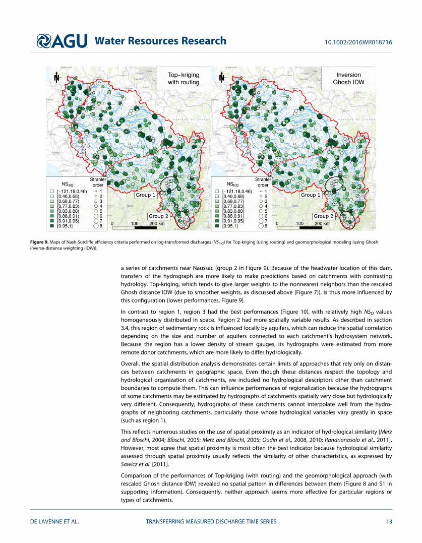
a series of catchments near Naussac (group 2 in Figure 9). Because of the headwater location of this dam,transfers of the hydrograph are more likely to make predictions based on catchments with contrastinghydrology. Top-kriging, which tends to give larger weights to the nonnearest neighbors than the rescaledGhosh distance IDW (due to smoother weights, as discussed above (Figure 7)), is thus more influenced bythis configuration (lower performances, Figure 9).

In contrast to region 1, region 3 had the best performances (Figure 10), with relatively high NSQ valueshomogeneously distributed in space. Region 2 had more spatially variable results. As described in section3.4, this region of sedimentary rock is influenced locally by aquifers, which can reduce the spatial correlationdepending on the size and number of aquifers connected to each catchment’s hydrosystem network.Because the region has a lower density of stream gauges, its hydrographs were estimated from moreremote donor catchments, which are more likely to differ hydrologically.

Overall, the spatial distribution analysis demonstrates certain limits of approaches that rely only on distan-ces between catchments in geographic space. Even though these distances respect the topology andhydrological organization of catchments, we included no hydrological descriptors other than catchmentboundaries to compute them. This can influence performances of regionalization because the hydrographsof some catchments may be estimated by hydrographs of catchments spatially very close but hydrologicallyvery different. Consequently, hydrographs of these catchments cannot interpolate well from the hydro-graphs of neighboring catchments, particularly those whose hydrological variables vary greatly in space(such as region 1).

This reflects numerous studies on the use of spatial proximity as an indicator of hydrological similarity [Merzand Bl€oschl, 2004; Bl€oschl, 2005; Merz and Bl€oschl, 2005; Oudin et al., 2008, 2010; Randrianasolo et al., 2011].However, most agree that spatial proximity is most often the best indicator because hydrological similarityassessed through spatial proximity usually reflects the similarity of other characteristics, as expressed bySawicz et al. [2011].

Comparison of the performances of Top-kriging (with routing) and the geomorphological approach (withrescaled Ghosh distance IDW) revealed no spatial pattern in differences between them (Figure 8 and S1 insupporting information). Consequently, neither approach seems more effective for particular regions ortypes of catchments.

Figure 9. Maps of Nash-Sutcliffe efficiency criteria performed on log-transformed discharges (NSlnQ) for Top-kriging (using routing) and geomorphological modeling (using Ghoshinverse-distance weighting (IDW)).

Water Resources Research 10.1002/2016WR018716

DE LAVENNE ET AL. TRANSFERRING MEASURED DISCHARGE TIME SERIES 13

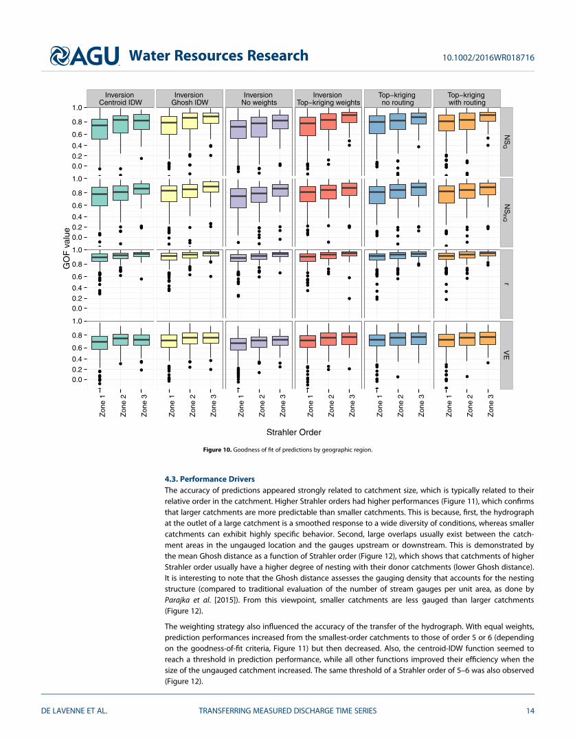
4.3. Performance DriversThe accuracy of predictions appeared strongly related to catchment size, which is typically related to theirrelative order in the catchment. Higher Strahler orders had higher performances (Figure 11), which confirmsthat larger catchments are more predictable than smaller catchments. This is because, first, the hydrographat the outlet of a large catchment is a smoothed response to a wide diversity of conditions, whereas smallercatchments can exhibit highly specific behavior. Second, large overlaps usually exist between the catch-ment areas in the ungauged location and the gauges upstream or downstream. This is demonstrated bythe mean Ghosh distance as a function of Strahler order (Figure 12), which shows that catchments of higherStrahler order usually have a higher degree of nesting with their donor catchments (lower Ghosh distance).It is interesting to note that the Ghosh distance assesses the gauging density that accounts for the nestingstructure (compared to traditional evaluation of the number of stream gauges per unit area, as done byParajka et al. [2015]). From this viewpoint, smaller catchments are less gauged than larger catchments(Figure 12).

The weighting strategy also influenced the accuracy of the transfer of the hydrograph. With equal weights,prediction performances increased from the smallest-order catchments to those of order 5 or 6 (dependingon the goodness-of-fit criteria, Figure 11) but then decreased. Also, the centroid-IDW function seemed toreach a threshold in prediction performance, while all other functions improved their efficiency when thesize of the ungauged catchment increased. The same threshold of a Strahler order of 5–6 was also observed(Figure 12).

Figure 10. Goodness of fit of predictions by geographic region.

Water Resources Research 10.1002/2016WR018716

DE LAVENNE ET AL. TRANSFERRING MEASURED DISCHARGE TIME SERIES 14

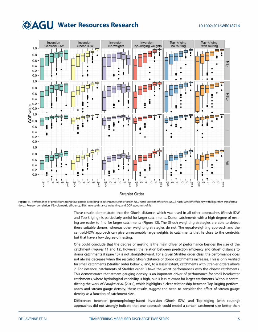
These results demonstrate that the Ghosh distance, which was used in all other approaches (Ghosh IDWand Top-kriging), is particularly useful for larger catchments. Donor catchments with a high degree of nest-ing are easier to find for larger catchments (Figure 12). The Ghosh weighting strategies are able to detectthese suitable donors, whereas other weighting strategies do not. The equal-weighting approach and thecentroid-IDW approach can give unreasonably large weights to catchments that lie close to the centroidsbut that have a low degree of nesting.

One could conclude that the degree of nesting is the main driver of performance besides the size of thecatchment (Figures 11 and 12); however, the relation between prediction efficiency and Ghosh distance todonor catchments (Figure 13) is not straightforward. For a given Strahler order class, the performance doesnot always decrease when the rescaled Ghosh distance of donor catchments increases. This is only verifiedfor small catchments (Strahler order below 2) and, to a lesser extent, catchments with Strahler orders above7. For instance, catchments of Strahler order 3 have the worst performances with the closest catchments.This demonstrates that stream-gauging density is an important driver of performance for small headwatercatchments, where hydrological variability is high, but is less relevant for larger catchments. Without contra-dicting the work of Parajka et al. [2015], which highlights a clear relationship between Top-kriging perform-ances and stream-gauge density, these results suggest the need to consider the effect of stream-gaugedensity as a function of catchment size.

Differences between geomorphology-based inversion (Ghosh IDW) and Top-kriging (with routing)approaches did not strongly indicate that one approach could model a certain catchment size better than

Figure 11. Performance of predictions using four criteria according to catchment Strahler order. NSQ: Nash-Suttcliff efficiency, NSlnQ: Nash-Suttcliff efficiency with logarithm transforma-tion, r: Pearson correlation, VE: volumetric efficiency, IDW: inverse-distance weighting, and GOF: goodness of fit.

Water Resources Research 10.1002/2016WR018716

DE LAVENNE ET AL. TRANSFERRING MEASURED DISCHARGE TIME SERIES 15

the others (Figure 11). Only the NSQ cri-teria appeared to demonstrate thatthe Top-kriging approach providedbetter results for smaller catchments(Strahler order� 2) than the geomor-phological approach. The high variabil-ity in hydrological behavior of smallcatchments seems better addressedby using a variogram instead of a sim-ple IDW approach with the Ghoshdistance.

Moreover, the geomorphologicalapproach is better suited to largercatchments. Indeed, hillslope traveltime tends to dominate the hydrologi-cal response for smaller catchments[D’Odorico and Rigon, 2003] even if it isa difficult task to say when it occursexactly [see for instance, Lazzaro et al.,2016; Rigon et al., 2016]. For this rea-son, as donor catchments get smaller,their network transfer function tendsto be shorter. The inversion then

Figure 12. Weighted mean rescaled Ghosh distance between receiver catch-ments and their five donor catchments. Weights are those used for transferringhydrographs.

Figure 13. Performance of simulation (using NSlnQ criteria) of receiver catchments according to the weighted mean rescaled Ghoshdistance to their five donor catchments. Weights are those used for transferring hydrographs.

Water Resources Research 10.1002/2016WR018716

DE LAVENNE ET AL. TRANSFERRING MEASURED DISCHARGE TIME SERIES 16

becomes insignificant because the net rainfall time series tends to be similar to the discharge time series.With insignificant inversion, hydrograph transfer in the two approaches becomes similar, and the main dif-ferences in performances can only be explained by weighting strategy, as described in the previousparagraph.

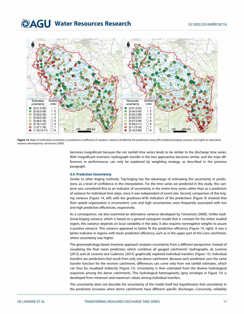
4.4. Prediction UncertaintySimilar to other kriging methods, Top-kriging has the advantage of estimating the uncertainty in predic-tions, as a level of confidence in the interpolation. For the time series we predicted in this study, this vari-ance was considered first as an indicator of uncertainty in the entire time series rather than as a predictionof variance for individual time steps, since it was independent of event size. Second, comparison of this krig-ing variance (Figure 14, left) with the goodness-of-fit indicators of the predictions (Figure 9) showed thattheir spatial organization is inconsistent. Low and high uncertainties were frequently associated with lowand high prediction efficiencies, respectively.

As a consequence, we also examined an alternative variance developed by Yamamoto [2000]. Unlike tradi-tional kriging variance, which is based on a general variogram model that is constant for the entire studiedregion, this variance depends on local variability in the data. It also requires nonnegative weights to assurea positive variance. This variance appeared to better fit the prediction efficiency (Figure 14, right). It was abetter indicator in regions with lower prediction efficiency, such as in the upper part of the Loire catchment,where uncertainty was higher.

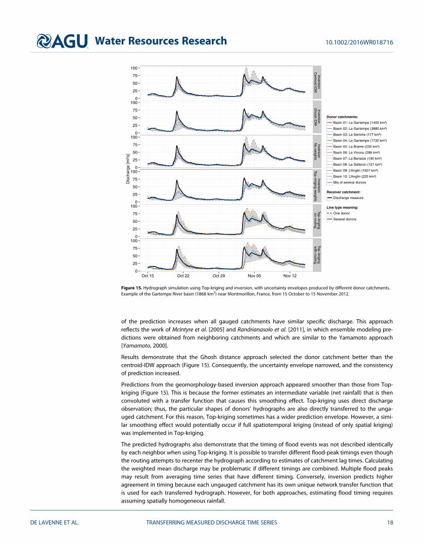
The geomorphology-based inversion approach analyzes uncertainty from a different perspective. Instead ofvisualizing the final mean prediction, which combines all gauged catchments’ hydrographs, de Lavenne[2013] and de Lavenne and Cudennec [2015] graphically explored individual transfers (Figure 15). Individualtransfers are predictions that result from only one donor catchment. Because each prediction uses the sametransfer function for the receiver catchment, differences can come only from net rainfall estimates, whichcan thus be visualized indirectly (Figure 15). Uncertainty is then estimated from the diverse hydrologicalresponses among the donor catchments. This hydrological heterogeneity (grey envelope in Figure 15) isdeveloped from minimum and maximum values among individual transfers.

This uncertainty does not describe the uncertainty of the model itself but hypothesizes that uncertainty inthe prediction increases when donor catchments have different specific discharges. Conversely, reliability

Figure 14. Maps of estimated uncertainty in predictions (coefficient of variation: variance divided by the prediction) using (left) traditional kriging variance and (right) an alternativevariance developed by Yamamoto [2000].

Water Resources Research 10.1002/2016WR018716

DE LAVENNE ET AL. TRANSFERRING MEASURED DISCHARGE TIME SERIES 17

of the prediction increases when all gauged catchments have similar specific discharge. This approachreflects the work of McIntyre et al. [2005] and Randrianasolo et al. [2011], in which ensemble modeling pre-dictions were obtained from neighboring catchments and which are similar to the Yamamoto approach[Yamamoto, 2000].

Results demonstrate that the Ghosh distance approach selected the donor catchment better than thecentroid-IDW approach (Figure 15). Consequently, the uncertainty envelope narrowed, and the consistencyof prediction increased.

Predictions from the geomorphology-based inversion approach appeared smoother than those from Top-kriging (Figure 15). This is because the former estimates an intermediate variable (net rainfall) that is thenconvoluted with a transfer function that causes this smoothing effect. Top-kriging uses direct dischargeobservation; thus, the particular shapes of donors’ hydrographs are also directly transferred to the unga-uged catchment. For this reason, Top-kriging sometimes has a wider prediction envelope. However, a simi-lar smoothing effect would potentially occur if full spatiotemporal kriging (instead of only spatial kriging)was implemented in Top-kriging.

The predicted hydrographs also demonstrate that the timing of flood events was not described identicallyby each neighbor when using Top-kriging. It is possible to transfer different flood-peak timings even thoughthe routing attempts to recenter the hydrograph according to estimates of catchment lag times. Calculatingthe weighted mean discharge may be problematic if different timings are combined. Multiple flood peaksmay result from averaging time series that have different timing. Conversely, inversion predicts higheragreement in timing because each ungauged catchment has its own unique network transfer function thatis used for each transferred hydrograph. However, for both approaches, estimating flood timing requiresassuming spatially homogeneous rainfall.

Figure 15. Hydrograph simulation using Top-kriging and inversion, with uncertainty envelopes produced by different donor catchments.Example of the Gartempe River basin (1868 km2) near Montmorillon, France, from 15 October to 15 November 2012.

Water Resources Research 10.1002/2016WR018716

DE LAVENNE ET AL. TRANSFERRING MEASURED DISCHARGE TIME SERIES 18

5. Discussion

5.1. Founding PrinciplesDespite having similar performances, Top-kriging and geomorphology-based inversion approaches differ intheir founding principles. Top-kriging adapts traditional kriging to hydrological support. It takes advantageof geostatistics that produce the best linear unbiased estimators (BLUE) [Journel and Huijbregts, 1978]. How-ever, these approaches assume stationarity, which is not fully respected over the spatiotemporal domain.Consequently, it may be necessary to create multiple variograms for each homogeneous region. Top-kriging thus mainly focuses on constructing a variogram model.

Conversely, the geomorphology-based inversion approach uses a model that is not based on a statisticaldescription of discharge but on a geomorphological description of each catchment. It uses a well-knownfamily of transfer functions and takes advantage of easily observable catchment features to provide a robustmodeling approach. It is also based on inverse-modeling techniques to estimate and use net rainfall as anintermediate variable, while Top-kriging predicts directly from discharge measurements. Net rainfall cannotbe compared to any measurements, which questions the physical meaning of the time series. Among otherissues, solutions of inverse models may be subject to oscillations.

Despite differences in how the methods were developed, they share certain properties that can explaintheir similar behaviors. Top-kriging point variograms examine properties of unobserved runoff generationat the point scale. This runoff generation can be seen as a different way to describe the net rainfall of thegeomorphology-based model. The approaches differ in that Top-kriging spatially convolutes statisticalproperties of net rainfall to find weights of runoff observations, whereas the geomorphology-basedapproach interpolates net rainfall directly and spatiotemporally convolutes it using the UH. We wouldexpect the geomorphology-based inversion approach, by using UH, to better predict the shape of hydro-graphs, but this was not detectable in the performance indicators.

5.2. Ease of ApplicationOne advantage of the geomorphology-based approach is that it can be applied using only a single neigh-bor (as originally designed) while still preserving certain characteristics of the ungauged catchment by con-voluting net rainfall with the UH. This can address many situations for points of interest, such as when onlyone station is within a practical range. Like any other geostatistical approach, Top-kriging needs an ade-quate number of catchments to estimate the variogram, but can, like all distance-based methods, alsomake a prediction based on a single neighbor. However, this prediction would reproduce exactly the samespecific discharge, possibly with a phase shift due to the routing routine, but without the shape shift thatcomes from using multiple UHs.

5.3. Flexibility and Perspectives for EvolutionIn terms of flexibility, Top-kriging has a nonnegligible advantage over the geomorphological approach.Top-kriging can easily be used to estimate flow statistics (and is more widely used for this purpose), where-as the geomorphological approach is mainly designed for interpolating time series. So far, the only way toestimate flow statistics using the geomorphological approach is to derive them from the predicted dis-charge. Further investigation is needed to know whether this approach would provide satisfactory results.

An intermediate variable, i.e., net rainfall, is the geomorphology-based approach’s solution to solve the scal-ing issue inherent in transfer of hydrographs between catchments of different sizes. This net rainfall canthen be transferred to neighboring catchments independent of scale. Top-kriging uses specific dischargeand regularizes the variogram to address the scaling issue.

Despite difficulties inherent in inverse modeling, estimating net rainfall from discharge measurements alsoopens new perspectives, such as corrections according to spatiotemporal rainfall variability [de Lavenne,2013]. This aspect can also be considered in Top-kriging, but only by using a spatiotemporal trend model[Montanari, 2005]. In contrast, net rainfall estimated from a geomorphology-based approach can be com-pared to rainfall measurements more directly.

It is also important to note that Top-kriging differs from the geomorphological approach by treating thedataset as a whole, by applying a global variogram model, whereas the geomorphological approach modelseach catchment more separately (even though it also uses a single method to estimate weights). Each

Water Resources Research 10.1002/2016WR018716

DE LAVENNE ET AL. TRANSFERRING MEASURED DISCHARGE TIME SERIES 19

catchment has its own transfer function that controls the shape of each simulated hydrograph. Conversely,Top-kriging predicts the shape of one hydrograph from the shapes of neighboring hydrographs, eventhough the routing in Top-kriging is adapted to individual catchments. Top-kriging focuses more on meas-urements, while the geomorphological approach requires more assumptions about modeling water transferat the catchment scale. It would be easy for it to use more advanced transfer functions, depending uponavailable knowledge and data. For instance, it can consider dispersion [Rinaldo et al., 1991] explicitly, where-as the Top-kriging approach considers this aspect more implicitly [Skøien et al., 2006; Skøien and Bl€oschl,2007].

With only a few improvements to include routing, the results also highlight that both approaches could bet-ter consider variability in flow velocity; however, other factors may be more important or easier to use. Forinstance, differences in runoff production are an important issue that has not yet been examined. Doing sowould require estimating hillslope behavior, which would mean using a much more complex hydrosystemmodel.

5.4. Common TraitsFinally, the results demonstrate that both approaches achieve similar performances when using the samedescription of distance between catchments, i.e., the Ghosh distance. However, the weights from Top-kriging did not improve performance when applied to the geomorphological model. Combining the simpleIDW approach with Ghosh distances provides performance similar to that of Top-kriging with a calibratedvariogram. This emphasizes that measuring distances between catchments (physically and hydrologically) isone of the most important aspects on which to focus.

The weakness of both approaches is apparent for small catchments, which have higher variability in hydro-logical behavior than larger catchments. Any approach that attempts to identify a similar catchment usingonly geographic distance has strong limitations. This can be partly solved with better understanding ofhydrological drivers; however, it is also likely that assumptions of homogeneous net rainfall in the geomor-phological approach and the generated runoff in the Top-kriging approach are less applicable for smallercatchments. For other methods, regionalization based on regression has the advantage of describing moreexplicitly catchment characteristics that are related to a specific expected hydrological response.

6. Conclusion

Among regionalization studies, only a few approaches transfer weighted time series observations to unga-uged locations. Driven by the idea of maximizing data assimilation with a minimum of model development,we compared two of these observation-based approaches for a large dataset of 389 catchments spreadover the Loire River basin, the largest French basin (110,000 km2 at the outlet of Mont-Jean-sur-Loire).

The first is the Top-kriging approach based on the work of Skøien et al. [2006] and Skøien and Bl€oschl [2007],which was applied in a slightly modified form using the rtop package. This method is often compared toother regionalization techniques, such as regression [Archfield et al., 2013; Laaha et al., 2014], for estimatingstatistical catchment characteristics, and the regionalized hydrological model, for predicting continuousstreamflow [Viglione et al., 2013; Parajka et al., 2015]. In these studies, Top-kriging outperformed otherregionalization approaches.

The second approach implemented, initiated by Cudennec [2000] in small semiarid Tunisian basins andrecently applied in France by de Lavenne et al. [2015], relies on inverting a robust geomorphology-basedtransfer function of runoff through the river network. This study demonstrates that both approaches can beapplied in a similar manner. They are similar in their need for calibration (with estimated streamflow veloci-ty) and in how distances (as a proxy of hydrological similarity) are calculated between one gauged and oneungauged catchment.

Despite these common traits, each approach emerges from a different school of thought. Top-kriging isbased on geostatistics and uses statistical correlation to optimize weights. In contrast, the second approachcomes from geomorphology-based hydrological modeling, widely used to make predictions about unga-uged catchments. It uses easily observable catchment characteristics to describe the hydrograph of eachcatchment separately. The ability to treat each catchment more individually than in Top-kriging makes it

Water Resources Research 10.1002/2016WR018716

DE LAVENNE ET AL. TRANSFERRING MEASURED DISCHARGE TIME SERIES 20

possible, in theory, to include different levels of knowledge for each catchment. It does not benefit, howev-er, from the strength of statistical optimization for choosing and weighting the donor catchment, which isthe key challenge in both approaches. The final results from predictions over 13 hydrological years demon-strate similar performances of both approaches, showing that the geomorphology-based inversionapproach is as reliable as the well-known Top-kriging approach. This was achieved despite the slightly sim-pler weighting function of the geomorphological approach based on Ghosh inverse-distance weighting.

This study emphasizes the advantage of the Ghosh distance [Ghosh, 1951; Gottschalk, 1993; Gottschalk et al.,2011] for choosing and weighting gauged catchments as donors of observed streamflow to ungauged loca-tions. The advantage of this weighting strategy differs from that in the study by Andr�eassian et al. [2012], inwhich the simple mathematical mean of the neighboring catchments performed better. This weightingstrategy appears particularly relevant for catchments with Strahler orders above five, i.e., in which nestedcatchment structures are more significant.

ReferencesAndr�eassian, V., J. Lerat, N. Le Moine, and C. Perrin (2012), Neighbors: Nature’s own hydrological models, J. Hydrol., 414, 49–58, doi:10.1016/

j.jhydrol.2011.10.007.Aouissi, J., J. C. Pouget, H. Boudhraa, G. Storer, and C. Cudennec (2013), Joint spatial, topological and scaling analysis framework of river-

network geomorphometry, G�eomorphol. Relief Processus Environ., 1, 7–16, doi:10.4000/geomorphologie.10082.Archfield, S. A., A. Pugliese, A. Castellarin, J. O. Skøien, and J. E. Kiang (2013), Topological and canonical kriging for design flood prediction

in ungauged catchments: An improvement over a traditional regional regression approach?, Hydrol. Earth Syst. Sci., 17, 1575–1588, doi:10.5194/hess-17-1575-2013.

Beven, K., and E. F. Wood (1993), Flow routing and the hydrological response of channel networks, in Channel Network Hydrology, pp.99–128, John Wiley, Chichester, U. K.

Bl€oschl, G. (2005), Rainfall-runoff modeling of ungauged catchments, in Encyclopedia of Hydrological Sciences, pp. 2061–2079, John Wiley,Hoboken, N. J., doi:10.1002/0470848944.hsa140.

Bl€oschl, G., and M. Sivapalan (1995), Scale issues in hydrological modelling: A review, Hydrol. Processes, 9, 251–290, doi:10.1002/hyp.3360090305.Bl€oschl, G., M. Sivapalan, T. Wagener, A. Viglione, and H. H. G. Savenije (2013), Runoff Prediction in Ungauged Basins. Synthesis Across Process-

es, Places and Scales, Cambridge Univ. Press, Cambridge, U. K.Boudhraa, H. (2007), Mod�elisation pluie-d�ebit �a base g�eomorphologique en milieu semi-aride rural tunisien: association d’approches

directes et inverses, PhD thesis, Inst. Natl. Agron. de Tunisie �a Tunis, Tunis, Tunisia.Boudhraa, H., C. Cudennec, M. Slimani, and H. Andrieu (2006), Inversion d’une mod�elisation de type hydrogramme unitaire �a base

g�eomorphologique: interpr�etation physique et premiere mise en oeuvre, IAHS Publ., 303, 3912399.Boudhraa, H., C. Cudennec, M. Slimani, and H. Andrieu (2009), Hydrograph transposition between basins through a geomorphology-based

deconvolution-reconvolution approach, IAHS Publ., 333, 76–83.Cressie, N. (1993), Statistics for Spatial Data: Wiley Series in Probability and Statistics, Wiley-Interscience, N. Y.Criss, R. E., and W. E. Winston (2008), Do Nash values have value? Discussion and alternate proposals, Hydrol. Processes, 22, 2723–2725, doi:

10.1002/hyp.7072.Cudennec, C. (2000), Description math�ematique de l’organisation du r�eseau hydrographique et mod�elisation hydrologique, PhD thesis,

Ecole Natl. Sup�erieure Agron. de Rennes, Rennes, France.Cudennec, C. (2007), On width function-based unit hydrographs deduced from separately random self-similar river networks and rainfall

variability: Discussion of ‘‘Coding random self-similar river networks and calculating geometric distances: 1. General methodology’’ and‘‘2. Application to runoff simulations,’’ Hydrol. Sci. J., 52, 230–237, doi:10.1623/hysj.52.1.230.

Cudennec, C., and Y. Fouad (2006), Structural patterns in river network organization at both infra- and supra-basin levels: The case of a gra-nitic relief, Earth Surf. Processes Landforms, 31, 369–381, doi:10.1002/esp.1275.

Cudennec, C., Y. Fouad, I. S. Gatot, and J. Duchesne (2004), A geomorphological explanation of the unit hydrograph concept, Hydrol. Pro-cesses, 18, 603–621, doi:10.1002/hyp.1368.

de Lavenne, A. (2013), Mod�elisation hydrologique �a base g�eomorphologique de bassins versants non jaug�es par r�egionalisation et trans-position d’hydrogramme, PhD thesis, Agrocampus-Ouest Rennes, Rennes, France.

de Lavenne, A., and C. Cudennec (2015), Prediction of streamflow from the set of basins flowing into a coastal bay, Proc. Int. Assoc. Hydrol.Sci., 365, 55–60, doi:10.5194/piahs-365-55-2015.

de Lavenne, A., C. Cudennec, and H. Boudhraa (2015), Streamflow prediction in ungauged basins through geomorphology-based hydro-graph transposition, Hydrol. Res., 46(2), 291–302, doi:10.2166/nh.2013.099.

D’Odorico, P., and R. Rigon (2003), Hillslope and channel contributions to the hydrologic response, Water Resour. Res., 39(5), 1113, doi:10.1029/2002WR001708.

Farmer, W. H. (2016), Ordinary kriging as a tool to estimate historical daily streamflow records, Hydrol. Earth Syst. Sci. Discuss., 2016, 1–23,doi:10.5194/hess-2015-536.

Ghosh, B. (1951), Random distances within a rectangle and between two rectangles, Bull. Calcutta Math. Soc., 43, 17–24.Giannoni, F., G. Roth, and R. Rudari (2003a), Can the behaviour of different basins be described by the same model’s parameter set? A geo-

morphologic framework, Phys. Chem. Earth, 28, 289–295, doi:10.1016/S1474-7065(03)00040-8.Giannoni, F., J. A. Smith, Y. Zhang, and G. Roth (2003b), Hydrologic modeling of extreme floods using radar rainfall estimates, Adv. Water.

Resour., 26, 195–203, doi:10.1016/S0309-1708(02) 00091-X.Gottschalk, L. (1993), Interpolation of runoff applying objective methods, Stochastic Hydrol. Hydraul., 7, 269–281, doi:10.1007/BF01581615.Gottschalk, L., E. Leblois, and J. O. Skøien (2011), Distance measures for hydrological data having a support, J. Hydrol., 402, 415–421, doi:

10.1016/j.jhydrol.2011.03.020.He, Y., A. B�ardossy, and E. Zehe (2011), A review of regionalisation for continuous streamflow simulation, Hydrol. Earth Syst. Sci., 15, 3539–

3553, doi:10.5194/hess-15-3539-2011.

AcknowledgmentsThis research was funded byEtablissement Public Loire, Agence del’eau Loire Bretagne, EuropeanRegional Development Fund, and the‘‘Eutrophisation-Trend ‘‘project. Thedischarge data used for this study arefreely provided by the French Banquehydro database (www.hydro.eaufrance.fr).

Water Resources Research 10.1002/2016WR018716

DE LAVENNE ET AL. TRANSFERRING MEASURED DISCHARGE TIME SERIES 21

Hrachowitz, M., et al. (2013), A decade of Predictions in Ungauged Basins (PUB)—A review, Hydrol. Sci. J., 58, 1198–1255, doi:10.1080/02626667.2013.803183.

Isaak, D. J., et al. (2014), Applications of spatial statistical network models to stream data, WIREs Water, 1, 277–294, doi:10.1002/wat2.1023.Jasiewicz, J., and M. Metz (2011), A new GRASS GIS toolkit for Hortonian analysis of drainage networks, Comput. Geosci., 37, 1162–1173,

doi:10.1016/j.cageo.2011.03.003.Journel, A. G., and C. J. Huijbregts (1978), Mining Geostatistics, Academic Press, London, U. K.Kyriakidis, P. C., and A. G. Journel (1999), Geostatistical space–time models: A review, Math. Geol., 31, 651–684, doi:10.1023/A:

1007528426688.Laaha, G., J. Skøien, and G. Bl€oschl (2014), Spatial prediction on river networks: Comparison of Top-kriging with regional regression, Hydrol.

Processes, 28, 315–324, doi:10.1002/hyp.9578.Lazzaro, M. D., A. Zarlenga, and E. Volpi (2016), Understanding the relative role of dispersion mechanisms across basin scales, Adv. Water

Resour., 91, 23–36, doi:10.1016/j.advwatres.2016.03.003.McIntyre, N., H. Lee, H. Wheater, A. Young, and T. Wagener (2005), Ensemble predictions of runoff in ungauged catchments, Water Resour.

Res., 41, W12434, doi:10.1029/2005WR004289.Menke, W. (1989), Geophysical Data Analysis: Discrete Inverse Theory, vol. 45, Academic Press, San Diego, Calif.Merz, R., and G. Bl€oschl (2004), Regionalisation of catchment model parameters, J. Hydrol., 287, 95–123, doi:10.1016/j.jhydrol.2003.09.028.Merz, R., and G. Bl€oschl (2005), Flood frequency regionalisation—Spatial proximity vs. catchment attributes, J. Hydrol., 302, 283–306, doi:

10.1016/j.jhydrol.2004.07.018.Montanari, A. (2005), Deseasonalisation of hydrological time series through the normal quantile transform, J. Hydrol., 313, 274–282, doi:

10.1016/j.jhydrol.2005.03.008.M€uller, M. F., and S. E. Thompson (2015), TopREML: A topological restricted maximum likelihood approach to regionalize trended runoff

signatures in stream networks, Hydrol. Earth Syst. Sci., 19, 2925–2942, doi:10.5194/hess-19-2925-2015.Naden, P. S. (1992), Spatial variability in flood estimation for large catchments: The exploitation of channel network structure, Hydrol. Sci. J.,

37, 53–71, doi:10.1080/02626669209492561.Nagel, D., J. M. Buffington, and C. Luce (2011), A simple drainage enforcement procedure for estimating catchment area using DEM data,

paper presented at NW GIS User Conference, Boise, Idaho, 17–21 Oct. [Available at http://boise2011.nwgis.org/sessions/simple-drainage-enforcement-procedure-estimating-catchment-area-using-dem-data.html.]

Nash, J. E. and J. V. Sutcliffe (1970), River flow forecasting through conceptual models part I — A discussion of principles, J. Hydrol., 10(3),282–290.

Oudin, L., V. Andr�eassian, C. Perrin, C. Michel, and N. Le Moine (2008), Spatial proximity, physical similarity, regression and ungaged catch-ments: A comparison of regionalization approaches based on 913 French catchments, Water Resour. Res., 44, W03413, doi:10.1029/2007WR006240.

Oudin, L., A. Kay, V. Andr�eassian, and C. Perrin (2010), Are seemingly physically similar catchments truly hydrologically similar?, WaterResour. Res., 46, W11558, doi:10.1029/2009WR008887.

Parajka, J., R. Merz, J. O. Skøien, and A. Viglione (2015), The role of station density for predicting daily runoff by Top-kriging interpolation inAustria, J. Hydrol. Hydromech., 63, 228–234, doi:10.1515/johh-2015-0024.

Patil, S., and M. Stieglitz (2012), Controls on hydrologic similarity: Role of nearby gauged catchments for prediction at an ungauged catch-ment, Hydrol. Earth Syst. Sci., 16, 551–562, doi:10.5194/hess-16-551-2012.

R Core Team (2015), R: A Language and Environment for Statistical Computing, R Found. for Stat. Comput., Vienna.Randrianasolo, A., M. H. Ramos, and V. Andr�eassian (2011), Hydrological ensemble forecasting at ungauged basins: Using neighbour catch-

ments for model setup and updating, Adv. Geosci., 29, 1–11, doi:10.5194/adgeo-29-1-2011.Rigon, R., M. Bancheri, G. Formetta, and A. de Lavenne (2016), The geomorphological unit hydrograph from a historical-critical perspective,

Earth Surf. Processes Landforms, 41, 27–37, doi:10.1002/esp.3855.Rinaldo, A., A. Marani, and R. Rigon (1991), Geomorphological dispersion, Water Resour. Res., 27, 513–525, doi:10.1029/90WR02501.Robinson, J. S., M. Sivapalan, and J. D. Snell (1995), On the relative roles of hillslope processes, channel routing, and network geomorpholo-

gy in the hydrologic response of natural catchments, Water Resour. Res., 31, 3089–3101, doi:10.1029/95WR01948.Rodriguez, F., C. Cudennec, and H. Andrieu (2005), Application of morphological approaches to determine unit hydrographs of urban

catchments, Hydrol. Processes, 19, 1021–1035, doi:10.1002/hyp.5643.Sauquet, E., L. Gottschalk, and I. Krasovskaia (2008), Estimating mean monthly runoff at ungauged locations: An application to France,

Hydrol. Res., 39, 403–423, doi:10.2166/nh.2008.331.Sawicz, K., T. Wagener, M. Sivapalan, P. A. Troch, and G. Carrillo (2011), Catchment classification: Empirical analysis of hydrologic similarity

based on catchment function in the eastern USA, Hydrol. Earth Syst. Sci., 15, 2895–2911, doi:10.5194/hess-15-2895-2011.Sivapalan, M., et al. (2003), IAHS Decade on Predictions in Ungauged Basins (PUB), 2003–2012: Shaping an exciting future for the hydrolog-

ical sciences, Hydrol. Sci. J., 48, 857–880, doi:10.1623/hysj.48.6.857.51421.Skøien, J. O., and G. Bl€oschl (2006), Catchments as space-time filters—A joint spatio-temporal geostatistical analysis of runoff and precipita-

tion, Hydrol. Earth Syst. Sci., 10, 645–662, doi:10.5194/hess-10-645-2006.Skøien, J. O., and G. Bl€oschl (2007), Spatiotemporal topological kriging of runoff time series, Water Resour. Res., 43, W09419, doi:10.1029/

2006WR005760.Skøien, J. O., R. Merz, and G. Bl€oschl (2006), Top-kriging—Geostatistics on stream networks, Hydrol. Earth Syst. Sci., 10, 277–287, doi:

10.5194/hess-10-277-2006.Skøien, J. O., G. Bl€oschl, G. Laaha, E. Pebesma, J. Parajka, and A. Viglione (2014), rtop: An R package for interpolation of data with a variable

spatial support, with an example from river networks, Comput. Geosci., 67, 180–190, doi:10.1016/j.cageo.2014.02.009.Tarantola, A., and B. Valette (1982), Inverse problems: Quest for information, J. Geophys., 50, 150–170.Vandewiele, G., C.-Y. Xu, and W. Huybrechts (1991), Regionalisation of physically-based water balance models in Belgium. Application to

ungauged catchments, Water Resour. Manage., 5, 199–208, doi:10.1007/BF00421989.Viglione, A., J. Parajka, M. Rogger, J. L. Salinas, G. Laaha, M. Sivapalan, and G. Bl€oschl (2013), Comparative assessment of Predictions in

Ungauged Basins—Part 3: Runoff signatures in Austria, Hydrol. Earth Syst. Sci., 17, 2263–2279, doi:10.5194/hess-17-2263-2013.Yamamoto, J. (2000), An alternative measure of the reliability of ordinary kriging estimates, Math. Geol., 32, 489–509, doi:10.1023/A:

1007577916868.Yang, D., S. Herath, and K. Musiake (2002), A hillslope-based hydrological model using catchment area and width functions, Hydrol. Sci. J.,

47, 49–65, doi:10.1080/02626660209492907.

Water Resources Research 10.1002/2016WR018716

DE LAVENNE ET AL. TRANSFERRING MEASURED DISCHARGE TIME SERIES 22