
Relationship between mass transfer of permeants and polymer processing

Transfer Function Analysis of Mechanoluminescent Polymer Composites
THESIS
Presented in Partial Fulfillment of the Requirements for the Honors Undergraduate Research
Distinction in The College of Engineering at The Ohio State University
By
Hugo van der Walt
Undergraduate Program in Mechanical Engineering
The Ohio State University
2016
Committee:
Dr. Vishnubaba Sundaresan, Advisor
Dr. Krishnaswamy Srinivasan

Copyright by
Hugo van der Walt
2016

ii
Abstract
Composite materials are increasingly used in automotive and aviation industries due to their
high strength-to-weight ratio. Unfortunately, stress/strain measurements and failure prediction
are complex due to anisotropic properties within composite materials. Systems such as ultrasonic
non-destructive testing and fiber optic methods are available; however, these methods are
expensive, fragile, and not compact. Therefore, these systems cannot be integrated into an
automotive chassis or airplane fuselage for real-time health monitoring. To overcome this
limitation, a mechanoluminescent (ML) phosphor can be used as an additive within composite
structures. Due to the ML phosphors, the material will emit light at an intensity proportional to
applied mechanical strain/stress or strain/stress-rate applied to the structure. However, current
literature does not include an understanding of the transient response of ML due to a tensile load.
The purpose of this work was to design a data acquisition system to obtain temporal luminance
(light intensity) measurements from elastomer coupons embedded with mechanoluminescent
copper doped phosphors. These measurements were then used to understand the frequency
response of the ML coupon. A mechanical shaker was used to apply tensile loadings to the
coupons and a photoresistor (PR) was used to measure the light intensity. The PR was calibrated
with a spectroradiometer and LED. Chirp signals were used to identify subsystem transfer
functions. Understanding the PR response, a numerical method was presented to obtain temporal
luminance response. The frequency response of a ML coupon was measured for the first time
and found to exhibit an increasing magnitude response with increasing strain frequency. The
developed data acquisition system and measured frequency response, have set the foundation for
a better understanding of the ML phenomenon and have been utilized to predict failure in a ML
coupon.

iii
Dedication
This thesis is dedicated to my family, and in memory of my brother, Hennie van der Walt.

iv
Acknowledgements
I would like to acknowledge Honda R&D Americas Inc. and NSF I/UCRC Smart Vehicle
Concept Center for supporting this project. Thank you specifically to Duane Detwiler and
Nichole Verwys from Honda R&D.
An enormous thanks goes to my advisor Dr. Sundaresan. His willingness to work with
me as an undergraduate student was humbling. I am thankful to all of his guidance,
encouragement, and support throughout this project.
I would like to acknowledge all of my colleagues in The Integrated Material Systems
Lab. A special thanks goes to Srivatsava Krishnan for his guidance and never ending willingness
to help. Thank you to Jacob Maddox for your positive attitude, being patient with me, and being
able to answer my constant barrage of questions.
I would especially like to thank my family for their love, encouragement, and
reassurances throughout this project and my life. I am thankful to God for opening this door in
my life and allowing me to serve him through this work.

v
Vita
Fall 2014 to present……………………………..Undergraduate Research Assistant,
Department of Mechanical and Aerospace
Engineering, The Ohio State University
Fields of Study
Major Field: Mechanical Engineering

vi
Table of Contents
Abstract ........................................................................................................................................... ii
Acknowledgements ........................................................................................................................ iv
Vita .................................................................................................................................................. v
Fields of Study ................................................................................................................................ v
Table of Contents ........................................................................................................................... vi
List of Tables ............................................................................................................................... viii
List of Figures ................................................................................................................................ ix
Chapter 1: Introduction ................................................................................................................... 1
1.1. Composites and Structural Health Monitoring ........................................................................ 1
1.2. Mechanoluminescence (ML) Phenomenon ............................................................................... 3
1.3. Elastico-Mechanoluminescence (EML) Transient Response .................................................. 5
1.4. Elastico-Mechanoluminescence Tensile Loading ..................................................................... 6
1.5. Focus of Research ....................................................................................................................... 8
Chapter 2: Design of Data Acquisition System (DAQ) ................................................................ 10
2.1 Photoresistor Sensor ................................................................................................................. 10
2.2 EML Coupons ........................................................................................................................... 13
2.3 System Setup .............................................................................................................................. 14
Chapter 3: Electrodynamic Shaker and Photoresistor Calibration ............................................... 16
3.1 Electrodynamic Shaker Calibration ........................................................................................ 16
3.1.1 Frequency Analysis ........................................................................................................... 17
3.2 Photoresistor Calibration ......................................................................................................... 19
3.2.1 Luminance Calibration ..................................................................................................... 20
3.2.2 Frequency Analysis ........................................................................................................... 25
3.3 Temporal Luminance Response .............................................................................................. 28
Chapter 4: System and EML Coupon Frequency Analysis .......................................................... 32
4.1 System Setup .............................................................................................................................. 32
4.2 System Frequency Response and Analysis ............................................................................. 33
4.3 EML Coupon Analysis ............................................................................................................. 34
Chapter 5: Conclusion................................................................................................................... 37
5.1 Contributions and Future Work ............................................................................................. 37

vii
Appendix A: Chapter 2
Appendix B: Chapter 3
Appendix C: Chapter 4
Appendix D: Matlab Code

viii
List of Tables
Table 1: Specifications of EML coupons used for testing. ........................................................... 13
Table 2: Shaker transfer function details. ..................................................................................... 18
Table 3: Photoresistor transfer function details. ........................................................................... 27

ix
List of Figures
Figure 1: Percent share of structural composites in commercial aircraft over time [4]. ................. 2
Figure 2: Luminance dependence on strain [10]. ............................................................................ 7
Figure 3: Luminance dependence on strain rate [10]. ..................................................................... 7
Figure 4: Photoresistor circuit diagram......................................................................................... 12
Figure 5: Photoresistor sensor, test fixture, and circuit setup. ...................................................... 12
Figure 6: Block diagram of data acquisition system. .................................................................... 14
Figure 7: Shaker and laser interferometer setup [10]. ................................................................... 17
Figure 8: Shaker bode plot with adjusted frequency response. .................................................... 19
Figure 9: LED luminance values at different supply voltages. ..................................................... 22
Figure 10: Photoresistor chirp experiment setup. ......................................................................... 22
Figure 11: Voltage drop from PR circuit due to different LED supply voltages. ......................... 23
Figure 12: Correlation between luminance and PR circuit voltage drop. ..................................... 23
Figure 13: Photoresistor circuit response to varying distances. .................................................... 24
Figure 14: Static luminance calibration dependence on distance and PR circuit voltage
measurement. ................................................................................................................................ 25
Figure 15: PR bode plot with first order one pole transfer function estimate. .............................. 27
Figure 16: PR bode plot with third order transfer function estimate. ........................................... 28
Figure 17: Normalized response of shaker input, PR circuit voltage response, and numerical
luminance response. ...................................................................................................................... 29
Figure 18: Numerical EML luminance response to 10 Hz, .5V shaker input. .............................. 30
Figure 19: PR circuit voltage response to 10 Hz, .5V shaker input. ............................................. 31
Figure 20: Setup of overall system experiment. ........................................................................... 33
Figure 21: Overall system frequency response. ............................................................................ 34
Figure 22: Experimental frequency response of EML coupon. .................................................... 36

Chapter 1: Introduction
1.1. Composites and Structural Health Monitoring
Composites are a class of materials designed through the combination of two or more
individual materials. The combination occurs in a manner where no chemical reaction occurs,
but the resulting composite exhibits improved material properties over the original materials.
These properties can be tailored through different combinations, the percent weight of materials
used, and the process in which the composites are formed. Two of the most appealing properties
are increased specific strength and corrosion resistivity. The increase in specific strength enables
composites to have a lower density than metals, while exhibiting the same, if not greater
strength. Composite’s corrosion resistance allows these materials to be implemented in
environments where metals would typically not perform well over time. These enhanced
properties make composites extremely appealing for commercial applications.
Commercial automotive and aviation industries have utilized composite materials since the
1950s. Boeing first implemented fiberglass components in their 707 model, whereas Chevrolet
used structural composite materials in the 1953 Corvette [1] [2]. Following these initial
applications, the two industries rapidly increased their use of structural composites. Figure 1
displays the exponential trend of composite use in the aviation industry. As seen in the figure,
Boeing’s 787 model consists of almost fifty percent structural composites. This usage of
composites in place of metallic structures led to twenty percent weight reduction of the aircraft
[3].

2
Figure 1: Percent share of structural composites in commercial aircraft over time as shown by L.
Catherine Brinson and the National Research Council of the National Academies [4].
Although composites contribute to improved properties and have been implemented in
commercial industries, they are still being rigorously studied. Due to the anisotropic properties,
conventional health monitoring methods cannot be implemented. Failure also commonly occurs
through a complicated mechanism of delamination. Delamination is the separation of the
different materials in the composite at their binding interfaces. This failure method can be
difficult to detect through visual inspection as the delamination can occur within the body of the
material. Our limited understanding of composites and the liability issues involved with
participating in the commercial sector require the structural health of composite components to
be closely monitored.
Structural health monitoring is a measurement process in which the functionality and
performance of a structure is recorded. Some of the main characteristic monitored in these
0
10
20
30
40
50
60
1970 1975 1980 1985 1990 1995 2000 2005 2010 2015
Com
posi
te C
om
ponen
ts (
%)
Year
Structural Composite Components in Comercial Aircraft

3
processes are: stress, strain, crack propagation, impact detection, corrosion, and delamination.
Monitoring these aspects can reduce cost and down time by predicting failures before they occur.
Designs can also be better understood, leading to improved future designs. Two of the current
techniques being used for structural health monitoring are fiber optics and ultrasonic
nondestructive testing. A type of fiber optic method, Fiber Bragg Grating, functions by
measuring the change in wavelength of light sent through an optical fiber embedded within a
structure. As the fiber is strained, a grating within the fiber refracts light differently producing a
proportional shift in the light’s wavelength [5]. On the other hand, ultrasonic testing functions by
measuring changes to ultrasonic waves as they permeate through the structure. These
measurements can consist of changes in the frequency, amplitude, or phase of the original signal.
Changes to these signals can then be correlated to strain, stress, and other structural health
monitoring aspects [6]. Unfortunately, fiber optics, ultrasonic testing, and other current structural
health monitoring techniques have some limitations. Three limitations to be highlighted are:
requirement of an external input, use of bulky and expensive equipment, as well as the inability
to perform in-situ, real-time measurements. A mechanoluminescent-based smart optical sensor
system has been proposed in previous work as a solution to the aforementioned limitations [7].
1.2. Mechanoluminescence (ML) Phenomenon
Light emission can be separated into two main categories: incandescence and
luminescence. Utilization of the incandescence phenomenon is inefficient as light emission is
due to thermal radiation caused by heating of the material. This method results in high energy
losses. On the other hand, luminescence is not caused by heating the material, but by the
excitation of electrons from stable configurations into unstable configurations. As the electrons

4
return to a stable state, they release energy in form of light. There are different methods to excite
the electrons from their stable configurations, primarily: electrical excitation, or excitation by an
external electrical energy source. Excitation can also be achieved through mechanical loading.
This thesis will focus on the luminance emission from mechanical input forces. This emission of
light by a material when it is stressed or fractured is referred to as mechanoluminescence (ML).
There are three main sub-categories of mechanoluminescence: elastico-
mechanoluminescence (EML), plastico-mechanoluminescence (PML), and fracto-
mechanoluminescence (FML). These categories correspond to the type of deformation imparted
on the material. For this research, the focus was on the EML phenomenon and its characteristics.
Concentrating on EML allows for structural health monitoring before the failure of the material,
as well as observation of cyclical and other stresses operating in the elastic region. Materials
which exhibit EML usually exhibit PML and FML and thus could be used to characterize
strains/stresses in these regions as well [7] [8].
Almost fifty percent of crystal compounds have been found to exhibit some form of
mechanoluminescence. For the specific case of ZnS:Mn, previous work have suggested a
piezoelectric origin for ML excitation [7]. During mechanical loading, the crystal structure is
deformed, creating a piezoelectric field. This field supplies electrons in the lower band levels
with enough energy to facilitate excitation to the conduction band. From the conduction band,
electrons fall back to lower, stable energy levels releasing energy in the form of light. Dopants in
the crystal add stable lower energy levels which can accept electrons. Falling to one of these
acceptor states releases less energy, thus altering the wavelength of photons emitted by the
material. This can be understood by the Plank-Einstein equation shown below, where 𝐸 is

5
energy, ℎ is Plank’s constant, and 𝑣 is frequency. The smaller energy gap will result in a lower
frequency of light and thus a higher wavelength in the visible range.
𝐸 = ℎ𝑣 (1)
Although, the mechanism behind ML may be understood, the response of ML to different
mechanical loading conditions needs to be better understood before it can be successfully
implemented as a structural health monitoring sensor. Specifically, the transient responses to
different loads needs to be characterized, as it was presented in the piezoelectric theory ML
excitation is dynamic and not static. A static strain on the crystal structure will not continuously
supply energy to elevate electrons to higher energy levels.
1.3. Elastico-Mechanoluminescence (EML) Transient Response
Understanding the transient response of EML due to different mechanical excitations is
vital to structural health monitoring applications as the response has been shown to be dynamic,
as discussed in the previous section. Furthermore, EML characteristics from different loading
conditions are important to understand in order to distinguish what type of forces are acting on a
structure. Previous research has observed transient ML emission due to: ultrasonic, impact,
compression, and torsional input conditions. Studies by Zhang et al. were performed on the first
three of these input conditions using CaZnOS:Mn2+ as their EML source and measured results
with a CCD camera and photomultiplier tube [9]. Their results included time response plots for
ultrasonic, impact, and compression loadings. In all cases the luminance increased sharply with
the applied excitation and then decreased upon removal of the input. For the impact response, the
decay time was found to be less than 2.3 seconds. In all three cases the luminance increased
linearly with an increase of the excitation magnitude. The compression condition also yielded a

6
linear response between the luminance emitted and the compression rate applied. Kim et al.
focused their work on the analysis of torque mechanical loadings [10]. From their work one can
observe the time response, as well as frequency analysis of EML due to torque inputs. The
frequency analysis results displayed a decrease in their system response as the rate of torque
applied was increased. The work presented here is only a small sample presenting evidence for
how EML is a viable sensing method for various mechanical loadings. Although various loading
conditions were presented, it is important to discuss EML due to tensile loading as well. This
discussion will be conducted separately in the following section.
1.4. Elastico-Mechanoluminescence Tensile Loading
Previously, EML studies completed with a tensile mechanical loading condition have
only included time averaged data and no temporal or dynamic response. Krishnan’s work has
focused on the tensile loading for EML materials. This work was conducted primarily with
ZnS:Cu and ZnS:Mn phosphors impregnated within an elastomeric matrix and actuated by a
mechanical shaker to induce sinusoidal tensile loadings. Measurements were conducted using a
spectroradiometer, which had very low temporal resolution. The time averaged measurements
collected presented important results towards understanding EML behavior. Krishnan found the
luminance emitted by the coupons were dependent on both the strain and the strain rate applied
[11]. The dependence on these factors can be seen in Figures 1 and 2 below.

7
Figure 2: Luminance dependence on strain [11].
Figure 3: Luminance dependence on strain rate [11].

8
Initial tensile loading temporal response work related to this thesis was also presented by
Krishnan [11]. For these experiments, a photoresistor sensor was used to measure relative light
intensity values in real-time. Using this equipment, a relative time-response of EML due to
tensile loading was presented for the first time. From this data an important contributing
hypothesis was presented. Details of the hypothesis can be found in Krishnan’s thesis [11].
Although vital knowledge was obtained from the current setup, more work was needed to
calibrate the equipment for a luminance response as well as understand the frequency response of
EML due to tensile loading.
1.5. Focus of Research
It has been shown how ML characteristics are favorable for use in the structural health
monitoring community as alternatives to the current methods. However, most of the research
done in the field of ML and structural health monitoring have used CCD cameras [9],
photomultiplier tubes [9] [12], or a spectroradiometer [11] [13] to measure luminance emissions.
Although these are highly calibrated and sensitive equipment, they are expensive, fragile, and
bulky. None of these current measurement systems are feasible for onsite, real-time
measurements. The first objective of this work is to design a data acquisition system to obtain
temporal luminance measurements from elastomer coupons embedded with mechanoluminescent
copper doped phosphors (ZnS:Cu). This system was designed to address the limitations of
current equipment. The system is inexpensive, robust, has few components with a small profile,
and allows for future integration within structures itself. The second goal of this research thesis
was to use the data acquisition system to understand the frequency response and develop a
transfer function between the input strain and luminance emitted. From this analysis, one is able

9
to better understand what strain and strain rate is applied to a structure through the emitted
luminance. This knowledge would allow for a greater understanding of EML dynamics and lay
the foundation for future work in the field.
The second chapter of this thesis presents the design of the data acquisition system.
Chapter 3 discusses the calibration of the photoresistor and electrodynamic shaker. The
frequency response of these systems will be discussed here as well as the individual system’s
corresponding fitted transfer function. Chapter 4 contains the setup and analysis of the overall
system as well as the EML coupon frequency analysis testing. Finally, the fifth chapter contains
contributions made to the field and future work.

10
Chapter 2: Design of Data Acquisition System (DAQ)
In chapter 1, the background and motivation for this work was presented. Previous work
in the structural health monitoring and ML fields were presented along with their limitations.
The following chapter presents the design of the data acquisition system used in attempt to
overcome the aforementioned limitations. The key component of the system, the photoresistor
light sensor, will be introduced along with the motivation behind using this sensor. Details of the
EML coupons will be briefly covered and the overall system setup will be presented. One
component not introduced is the electrodynamic shaker used to supply the mechanical loading to
the coupons. Further information on the shaker can be found from the data sheet in Appendix A,
Figure A1.
2.1 Photoresistor Sensor
The first step in designing the DAQ was to determine what type of light sensor to use.
Numerous calibrated photodiodes and sensor systems are available on the market; however,
these sensors and systems lack the possibility of integration within a structure to create a smart,
self-sensing material. As previously mentioned in the introduction, it is desirable to design an
inexpensive, and robust system in a small profile. Therefore, in order to meet all of the
constraints, one of the most basic light sensing sensors was selected: a photoresistor.
Photoresistors (PR) are sensors which have a resistance proportional to the intensity of light
incident on the surface of the cell. A CdS based semiconductor PR was used. As the surface of

11
the sensor is exposed to light, the electrons in the valence band of the semiconductor receive
energy to jump to the conduction band. Free to move in the conduction band, the effective
resistance of the material is decreased. As more intense light is exposed to the surface, more
energy is introduced to the material. This facilitates more electron movement to the conduction
band, reducing the resistance even more.
Due to the resistive properties of the photoresistor, a voltage divider circuit was
constructed in order to measure a change in voltage proportional to the change in resistance. A
constant supply of 5V was selected because it is an accepted supply voltage standard and due to
limitations of the data acquisition board. The 5V was supplied through the use of a DC power
supply. As the light intensity exposed to the PR increases, the resistance decreases, leading to a
decrease in the voltage drop. It was desired to present a more intuitive measurement value which
would increase as the light intensity increased. Therefore, the voltage drop across the series
resistor was measured as this values increases with luminance. A diagram of the circuit can be
found in Figure 4 below. A Wheatstone bridge circuit could have been used, but the voltage
divider circuit was desired for its simplicity and reduced component count. This selection was
made with the possibility of future smart material implementation in consideration. The value of
the resistor in series with the photoresistor was determined next. Resistance values were taken
with the photoresistor exposed to ambient light and no light. A resistance value close to the
average of these measurements, 20 kΩ, was chosen in order yield an operating range within that
of average ambient light. In order to position the sensor in the desired location relative to EML
coupons, a fixture was designed and 3-D printed. Figure 5 below shows the photoresistor sensor
setup with the test fixture.

12
Figure 4: Photoresistor circuit diagram.
Figure 5: Photoresistor sensor, test fixture, and circuit setup.
Photoresistor circuit
Photoresistor setup and fixture
VDC= 5V
V
RS= 20 kΩ
PR Sensor
Vin

13
Photoresistors are mass produced, inexpensive, and readily available devices. The
photoresistor used in these experiments was purchased from RadioShack in a package of five
sensors for $3.99. A datasheet for the purchased photoresistor can be found in Appendix A,
Figure A2. Due to their inexpensive and mass manufactured nature, these components are not
highly calibrated, but will be assumed to be very repeatable. The calibration procedure and
results will be presented in Chapter 3.
2.2 EML Coupons
ZnS:Cu ML phosphors and a polydimethylsiloxane (PDMS) polymer were used to create the
EML coupons studied. These coupons were used to maintain consistency with previous
luminance measurements conducted within our lab. The composite formed from the combination
of these two components served as an initial tool to study EML before a more complicated
analysis is performed of a three part composite (polymer, reinforcement, and EML phosphor). A
SEM image of the coupon cross section can be found in Appendix A, Figure A3. The coupons
were formed using a method thoroughly discussed in Krishnan’s thesis [11]. Specifications of the
coupon used can be found in Table 1 below.
Table 1: Specifications of EML coupons used for testing.
Specification Value
ML Phosphor to PDMS Weight Ratio 7:3
Length (mm) 37
Width (mm) 10
Thickness (mm) 1.5

14
2.3 System Setup
Other components used in experiments were a: commercial computer, dSpace acquisition
board, light emitting diode (LED), and spectroradiometer. The computer and dSpace board were
primarily used for data collection and analysis. The dSpace board was also used to send
controlled inputs to the mechanical shaker and LED. A DS1104 R&D dSpace board was used
and the specification sheet can be found in Appendix A, Figure A4. The LED and
spectroradiometer will be discussed in future calibration sections. A complete system was design
comprised of all the aforementioned components. Figure 6 contains a diagram of the system in
order to understand the flow of information. First, a voltage signal is sent from the dSpace board
to the shaker. The shaker amplifies this signal and then actuates, displacing the attached EML
coupon. This displacement induces strain and stress in the EML coupon. Through the
piezoelectricity-induced EML model discussed in the introduction, light is emitted from the
coupon. Within close proximity, the photoresistor is exposed to the light, causing a change in its
resistance. The change in the photoresistor’s resistance alters the voltage drop across the resistor
in series with the photoresistor. This voltage drop is measured using the dSpace board.
Figure 6: Block diagram of data acquisition system.
dSpace Command
Shaker TF Coupon TF Photoresistor TFdSpace DAQ
Board
Input Voltage Signal
Displacement of Coupon
(Strain) Emitted Light
Voltage Proportional to Light Intensity

15
From the system diagram above, it is desired to obtain the transfer function (TF) of the
EML coupon. However, this relationship cannot be measured directly. In order to obtain this TF,
the whole system needs to be understood, as well as all the sub-systems. Therefore, frequency
analyses must first be performed on the PR, mechanical shaker, as well as the entire system. The
calibration and frequency analysis of the mechanical shaker and PR, will be completed in the
following chapter. Chapter 4 will contain the frequency analysis of the entire system along with
the analysis of the EML coupon.

16
Chapter 3: Electrodynamic Shaker and Photoresistor Calibration
Chapter 2 presented the design of the data acquisition system used to conduct the
temporal and frequency response measurements. The different components of the system were
introduced and the flow of information through the system was defined. In the following chapter,
an in-depth study of the electrodynamic shaker and the photoresistor will be outlined and
discussed. A frequency analysis was performed for both components and additional static
analysis was performed on the PR. A temporal response for the luminance of the EML coupon is
presented at the end of the chapter. For each calibration analysis, the setup and methods used will
be presented, followed directly by the results and a discussion.
3.1 Electrodynamic Shaker Calibration
The following section discusses the frequency analysis of the electrodynamic shaker used
to strain the ML coupons. The measurements for this study were conducted by Krishnan. During
the experiment, the shaker’s arm was not attached to an EML coupon. The free boundary
condition emphasizes this analysis only applies to the shaker itself. Further studies are needed to
understand how the dynamics of the shaker change with different boundary conditions.

17
3.1.1 Frequency Analysis
To understand the dynamics of the shaker, a transfer function was developed between the
voltage sent to the shaker (input) and corresponding displacement (output). The transfer function
desired from this analysis can be found in Equation 2 below. For this and following transfer
functions, the transfer function of the system is define as the output over the input of the system.
To accurately measure the displacement of the shaker arm, a HL-G103-A-C5 Compact Laser
Displacement Sensor was used. In this analysis it was assumed the laser interferometer was a
zeroth order component and did not influence the frequency response of the measurements.
Thus, a static calibration of .9mm/V was used to convert the laser interferometer voltage to
displacement. Due to range limitations of the laser, the shaker was placed 3cm away and
operated with a small amplitude. A schematic of the setup can be found in Figure 7.
(2)
Figure 7: Shaker and laser interferometer setup [11].
𝐺𝑆(𝑠) =𝑂𝑢𝑡𝑝𝑢𝑡(𝑠)
𝐼𝑛𝑝𝑢𝑡(𝑠)=
𝛿𝑆 (𝑚𝑚)
𝑉𝑆 (𝑉)
18
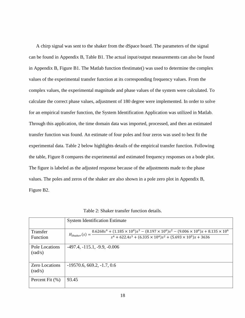
A chirp signal was sent to the shaker from the dSpace board. The parameters of the signal
can be found in Appendix B, Table B1. The actual input/output measurements can also be found
in Appendix B, Figure B1. The Matlab function tfestimate() was used to determine the complex
values of the experimental transfer function at its corresponding frequency values. From the
complex values, the experimental magnitude and phase values of the system were calculated. To
calculate the correct phase values, adjustment of 180 degree were implemented. In order to solve
for an empirical transfer function, the System Identification Application was utilized in Matlab.
Through this application, the time domain data was imported, processed, and then an estimated
transfer function was found. An estimate of four poles and four zeros was used to best fit the
experimental data. Table 2 below highlights details of the empirical transfer function. Following
the table, Figure 8 compares the experimental and estimated frequency responses on a bode plot.
The figure is labeled as the adjusted response because of the adjustments made to the phase
values. The poles and zeros of the shaker are also shown in a pole zero plot in Appendix B,
Figure B2.
Table 2: Shaker transfer function details.
System Identification Estimate
Transfer
Function 𝐻𝑆ℎ𝑎𝑘𝑒𝑟(𝑠) =
0.6268𝑠4 + (1.185 × 10⁴)𝑠3 − (8.197 × 10⁶)𝑠2 − (9.006 × 10⁶)𝑠 + 8.135 × 10⁶
𝑠4 + 622.4𝑠3 + (6.335 × 10⁴)𝑠2 + (5.693 × 10⁵)𝑠 + 3636
Pole Locations
(rad/s)
-497.4, -115.1, -9.9, -0.006
Zero Locations
(rad/s)
-19570.6, 669.2, -1.7, 0.6
Percent Fit (%) 93.45

19
Figure 8: Shaker bode plot with adjusted frequency response.
It is important to note there is a positive zero in the estimated transfer function. This
characterizes the transfer function as a non-minimum phase system and helps explain the large
change in phase. From the bode plot, deviation between the estimate and experimental data is
observed at high frequencies. Thus, the estimate can only be accurately used for low frequencies.
Due to the complexity and boundary condition used in analysis of this system, a numerical
technique to counteract the effects of the system was not developed. The Matlab code used to
compute the result for this section can be found in Appendix D, in Code 1.
3.2 Photoresistor Calibration
The following sections discuss the procedure and results obtained from the photoresistor
calibrations. First, the static luminance calibration with the PR, an LED, and a spectroradiometer

20
are explained. Next, a frequency analysis was performed to understand the dynamic
contributions and limitations of the PR sensor. Two transfer function estimations are presented,
along with a first order numerical method used to obtain a temporal luminance response.
3.2.1 Luminance Calibration
Measuring the voltage drop from the PR circuit presents an understanding of the relative
light intensity incident on the photoresistor. In order to obtain absolute measurements, calibration
was required. For this calibration, the SI derived unit of luminance was used, 𝑐𝑑
𝑚2. Luminance is
measurement of the luminous intensity over a given area. A spectroradiometer and LED were
used to perform these calibrations.
The spectroradiometer used was a Photo Research SpectraScan PR-655. The device was
previously used to characterize the time averaged response of EML coupons in Krishnan’s work.
This calibrated device is capable of measuring luminance, wavelength, and other photometric
quantities. In order to supply constant and controlled light intensity, an LED was used. In order
to limit the effect of varying wavelength on the PR response, it was important to use an LED
with a similar peak wavelength as the EML coupons. Previous research found the wavelength of
ZnS:Cu coupons to be 512 nm [11]. An LED rated at 510 nm was then purchased from Jameco
to closely match this wavelength. The data sheet for the LED can be found in Appendix B,
Figure B3. In order to understand the variation in wavelength of the LED, the spectroradiometer
was used to record the wavelength of the LED at different LED supply voltages. The LED was
placed in series with a 200 Ω resistor during operation. The wavelength dependence of the LED
over the voltage range of interest can be found in Appendix B, Figure B4. In this figure,

21
deviations of 4nm are randomly observed. These variations are due to the 4nm resolution of the
spectroradiometer. Thus, it was assumed the wavelength of the LED did not affect the PR
response.
The static calibration of the photoresistor was completed through a three step process
detailed below.
1. The LED and spectroradiometer were used to determine the luminance values
corresponding to different LED supply voltages. Throughout calibration, the LED
was controlled though the dSpace board and the spectroradiometer was controlled
through custom Matlab code. Results of this calibration are shown in Figure 9 with a
fitted double exponential curve.
2. The LED and photoresistor were used to quantify the relationship between LED
supply voltage and the voltage drop measured from the PR circuit. During this
process, the distance between the two components was 15 mm. A setup of this
experiment can be found in Figure 10. Results of this calibration are shown in Figure
11.
3. These two data sets were used to define the correlation between luminance and
voltage drop across the photoresistor. Results are shown in Figure 12 with a linear fit.

22
Figure 9: LED luminance values at different supply voltages.
Figure 10: Photoresistor chirp experiment setup.
Photoresistor
LED
𝑦(𝑥) = (−3.237 ∗ 10−43)𝑒45.71𝑥 + (5.389 ∗ 10−29)𝑒31.43𝑥

23
Figure 11: Voltage drop from PR circuit due to different LED supply voltages.
Figure 12: Correlation between luminance and PR circuit voltage drop (𝑅2 = .99).
𝑦(𝑥) = 126.997𝑥 + 0.563

24
During step two of the calibration process, the LED was held 15 mm from the
photoresistor. Although this distance was arbitrarily chosen, a distance calibration was also
completed in order to compensate for the distance between the photoresistor and light sources in
the future. This experiment was completed by sending a constant voltage to the LED and
adjusting the distance between the PR and the LED. Figure 13 displays experimental data as well
as a linear fit. Using this data, as well as the data obtain from the luminance calibration, a new
relationship was developed. Equation 3 displays the static luminance expected as a function of
the distance between the PR and its light source, as well as the voltage drop measured from the
PR circuit. Following this equation is a 3-D plot over the regions of interest is shown in Figure
14. The Matlab code used to compute the result for this section can be found in Appendix D, in
Code 2, 3, and 4, respectively.
Figure 13: Photoresistor circuit response to varying distances.
𝑦(𝑥) = −0.03417𝑥 + 4.592

25
𝐿(𝑉𝑃𝑅 , 𝑑𝑡𝑒𝑠𝑡) = 126.997[(𝑉𝑃𝑅) − .03417(15𝑚𝑚 − 𝑑𝑡𝑒𝑠𝑡)] + .5631 [𝑐𝑑
𝑚2] (3)
Figure 14: Static luminance calibration dependence on distance and PR circuit voltage
measurement.
3.2.2 Frequency Analysis
For this experiment the same setup was used as the static calibration between the PR and
the LED. Figure 10 contains this setup. The desired transfer function of the system to be obtained
from this analysis can be found Equation 4. To analyze the frequency effects of this system, a
chirp signal was sent as an input to the LED from dSpace. The voltage drop across the
photoresistor was measured as the output. During this analysis it was assumed the frequency
effects from the LED were negligible and it was taken to be a zeroth order component. The

26
parameters of the chirp signal can be found in Appendix B, Table B2. The voltage values
supplied to the LED for the chirp signal were larger than the previously calibrated range in order
to help limit noise to the system during the dynamic response. However, this resulted in values
outside the bounds of the original luminance calibration for the LED. A second calibration curve
for the chirp signal LED supply voltage was calculated and is presented in Appendix B, Figure
B5. All of these results were collected through dSpace and analyzed in Matlab. The code for this
new calibration can be found in Appendix D, Code 3.
𝐺𝑃𝑅(𝑠) =𝑂𝑢𝑡𝑝𝑢𝑡(𝑠)
𝐼𝑛𝑝𝑢𝑡(𝑠)=
𝑉𝑃𝑅(𝑉)
𝐿𝐿𝐸𝐷 (𝑐𝑑𝑚2)
(4)
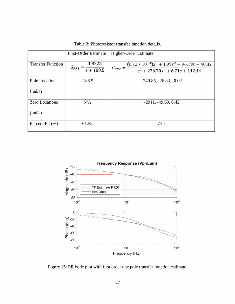
The actual input and output signals for the chirp experiment can be found in Appendix B,
Figure B6. The same procedure used to determine the experimental frequency results and the
empirical transfer function as for the shaker. Two estimates were found to represent the
photoresistor system. First, a simple first-order estimate was calculated consisting of one pole.
Second, a higher-order system of three poles and three zeros was calculated. The first-order
system was used to construct a model of the photoresistor and gain a more intuitive
understanding of how the sensor affects measurements at different frequencies. The higher-order
system resulted in a better fit to experimental data and was therefore used for further frequency
calculations. Table 3 below presents the empirical transfer functions, their pole and zero
locations, along with the percent fit determined from the System Identification Application.
Following the table, Figure 15 and Figure 16 present the estimated and experimental bode plots
for the first and third order systems, respectively. The pole and zero plot for the third order
estimate can be found in Appendix B, Figure B7.
27
Table 3: Photoresistor transfer function details.
First-Order Estimate Higher-Order Estimate
Transfer Function 𝐺𝑃𝑅1 =
1.8228
𝑠 + 188.5 𝐺𝑃𝑅2 =
(6.72 ∗ 10−4)𝑠3 + 1.99𝑠2 + 96.19𝑠 − 40.32
𝑠3 + 276.70𝑠2 + 6.71𝑠 + 142.44
Pole Locations
(rad/s)
-188.5 -249.85, -26.83, -0.02
Zero Locations
(rad/s)
N/A -2911, -49.60, 0.42
Percent Fit (%) 61.52 73.4
Figure 15: PR bode plot with first order one pole transfer function estimate.

28
Figure 16: PR bode plot with third order transfer function estimate.
From these plots, it can be observed the response of the PR sensor decreases as the
frequency of the light it is exposed to increases. The phase lag introduced by the sensor also
increases as the light intensity frequency increases. With the estimated transfer function, these
effects can be negated and removed from measurement data. The following section details the
approach used to accomplish this task and the results obtained.
3.3 Temporal Luminance Response
Using the first order transfer function estimate, a time domain differential equation was
found representative of the PR dynamics. Using this differential equation, the effects of the PR
can be removed from measurement data. The differential form of the TF is shown below in
Equation 5. Although EML measurements will be thoroughly discusses in the next chapter, a

29
sample measurement will be shown here. A sample measurement of the PR circuit voltage
response to EML excitation at 10 Hz can be seen in Figure 17. The luminance response, with the
PR dynamics removed, is also shown in Figure 17. In order to present both data sets on the same
plot, the values were normalized. It can be seen that the PR introduced a slight phase lag, as
expect from the frequency response analysis.
𝐺𝑃𝑅(𝑠) =𝑉𝑃𝑅(𝑠)
𝐿(𝑠)=
1.8228
𝑠 + 188.5= 𝑉𝑃𝑅(𝑠)[𝑠 + 188.5] = 𝐿(𝑠)[1.8228]
(5)
→1
1.8228[𝑑𝑉𝑃𝑅(𝑡)
𝑑𝑡+ 188.5𝑉𝑃𝑅(𝑡)] = 𝐿(𝑡)
Figure 17: Normalized response of shaker input, PR circuit voltage response, and numerical
luminance response.
Figure 18 below displays only the calibrated temporal luminance data. It is important to
note this is the first time temporal luminance data has been reported for EML due to tensile

30
loading. However, this analysis does not take into account the effects of the electrodynamic
shaker on the EML response. Further work in this field is needed in order to understand the
complex dynamics of the shaker when it is actuating a coupon. Dynamics of the shaker are
assumed to be coupled with the EML coupon due to its hyper-elastic nature. However, a
rough comparison can be drawn between the static and dynamic readings. Using the static
calibration, presented earlier, and the PR circuit response shown in Figure 19, a luminance
range of 20-40 𝑐𝑑
𝑚2 is expected. Even though this analysis does not account for any frequency
effects, the values are similar to the numerical temporal response, 18-37𝑐𝑑
𝑚2.
Figure 18: Numerical EML luminance response to 10 Hz, .5V amplitude shaker input.

31
Figure 19: PR circuit voltage response to 10 Hz, .5V amplitude shaker input.
32
Chapter 4: System and EML Coupon Frequency Analysis
Chapter 3 presented detailed frequency response analysis of the electrodynamic shaker
and the PR sensor. Static calibrations results were also showed. Finally, a temporal analysis of
the luminance measured by the PR sensor was displayed for the first time. Chapter 4 continues
on to analyze the overall measurement system and presents a numerical method to determine the
experimental frequency response of the EML coupon.
4.1 System Setup
In order to understand the frequency response of the EML coupon, an analysis of the entire
system was required. The EML coupon was placed between the shaker and the clamp in a zero
pre-strain condition. This was done to be consistent with previous analysis performed by
Krishnan. For this overarching analysis, the measured output was the voltage drop from the PR
circuit and the input was the voltage sent to the electrodynamic shaker. A chirp signal was used
as the input signal to the shaker. The parameters of the chirp signal can be found in Appendix C,
Table C1. For this experiment the chirp signal was only ran up to 17.5 Hz to ensure the coupons
would not break. This frequency range also limited the total number of cycles the EML coupon
experienced, reducing aging effects. Using these inputs and outputs, the frequency response for
the transfer function shown in Equation 6 was found. A figure displaying the layout of the setup
can be found in Figure 20. The actual input signal and output measurement can be found in
Appendix C, Figure C1.

33
𝐺𝑠𝑦𝑠𝑡𝑒𝑚(𝑠) =𝑂𝑢𝑡𝑝𝑢𝑡(𝑠)
𝐼𝑛𝑝𝑢𝑡(𝑠)=
𝑉𝑃𝑅 (𝑉)
𝑉𝑆 (𝑉)
(6)
Figure 20: Setup of overall system experiment.
4.2 System Frequency Response and Analysis
Using the Matlab code found in Appendix D, Code 7, the frequency response of the entire
measurement system was determined. The experimental data is shown in the bode plot in Figure
21. An attempt was made to determine an estimate of the transfer function for the system.
However, the system exhibited nonlinear properties. Determining a non-linear transfer function
was outside the scope of this analysis and could be further investigated in the future. Although a
numerical transfer function could not be determined, the experimental magnitude and phase data
Stationary Clamp
Composite Coupon Shaker (actuation)
Photoresistor

34
was used to determine the experimental frequency response of the EML coupon. This analysis
will be discussed in the following section.
Figure 21: Overall system frequency response.
4.3 EML Coupon Analysis
With magnitude and phase data for each sub-system and the overall system, enough
information was obtained in order to determine the response of the EML coupon. For the
following analysis, only the experimental measurements were used as a numerical estimate of the
entire system’s transfer function could not be calculated. Equation 7 shows how the known data
can be manipulated in order to determine the EML coupon’s response. The response of the
coupon has luminance as an output and displacement of the electrodynamic shaker as the input.
This displacement correlates to the displacement of the coupon and thus the actual strain
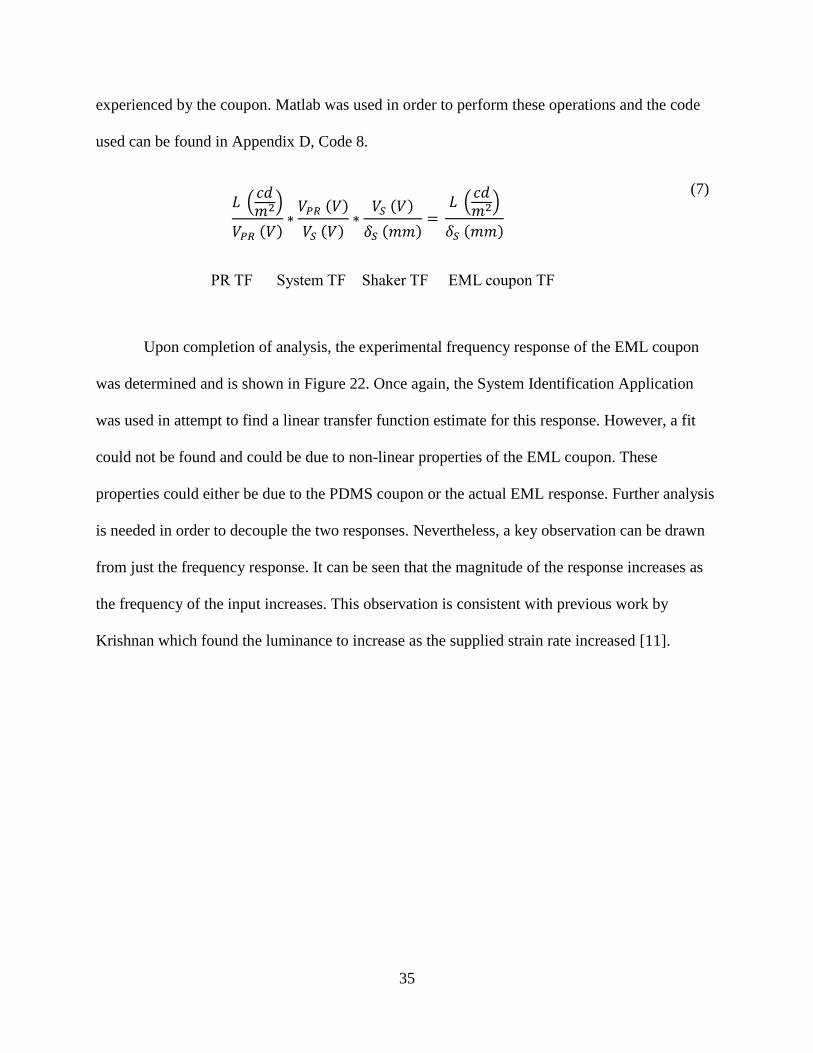
35
experienced by the coupon. Matlab was used in order to perform these operations and the code
used can be found in Appendix D, Code 8.
(7)
Upon completion of analysis, the experimental frequency response of the EML coupon
was determined and is shown in Figure 22. Once again, the System Identification Application
was used in attempt to find a linear transfer function estimate for this response. However, a fit
could not be found and could be due to non-linear properties of the EML coupon. These
properties could either be due to the PDMS coupon or the actual EML response. Further analysis
is needed in order to decouple the two responses. Nevertheless, a key observation can be drawn
from just the frequency response. It can be seen that the magnitude of the response increases as
the frequency of the input increases. This observation is consistent with previous work by
Krishnan which found the luminance to increase as the supplied strain rate increased [11].
𝐿 (𝑐𝑑𝑚2)
𝑉𝑃𝑅 (𝑉)∗
𝑉𝑃𝑅 (𝑉)
𝑉𝑆 (𝑉)∗
𝑉𝑆 (𝑉)
𝛿𝑆 (𝑚𝑚)=
PR TF System TF Shaker TF EML coupon TF
𝐿 (𝑐𝑑𝑚2)
𝛿𝑆 (𝑚𝑚)

36
Figure 22: Experimental frequency response of EML coupon.

37
Chapter 5: Conclusion
5.1 Contributions and Future Work
Through this work, several key contributions were made and are presented in the list below.
1. An inexpensive, robust, and minimal component system was measurement system was
designed which could lead to implementation into a future smart material.
2. It was shown the aforementioned system could be used to report temporal luminance
data.
3. The system was successfully used to present the first temporal EML response to tensile
loading.
4. The frequency response of an EML coupon was presented for the first time.
5. Through other work by the Integrated Material Systems Lab, the measurement system
was used to predict failure in an EML coupon.
The presented work and system have potential for numerous applications, but the most
promising would be to predict and understand failure in composite structures. Using the current
system and the failure analysis work, an algorithm could be developed to predict and warn of
impending failure. Future work could also focus on the analysis of the electrodynamic shaker’s
frequency response under different boundary conditions. With this understanding a more
accurate representation of the system could be determined. Future work in this field could be
focused on non-linear studies in order to obtain numerical transfer function estimates of the EML
coupon’s response. Similar experiments could be conducted using a more complicated composite
material containing fiber reinforcements and observing their response. Finally, future work could

38
focus on the integration of this technology within a structure to create a self-sensing smart
material.

39
References
[1] D. A. Day, "Composites and Advanced Materials," U.S. Centennial of Flight Commission .
[Online].
[2] J. Carruthers, E. Mangino and G. Patarresi, "The future use of structural composite
materials in the automotive industry," International Journal of Vehicle Design, p. 4, 2007.
[3] J. Hale, "Boeing 787 from the Ground Up," AERO, p. 4, 2006.
[4] L. C. Brinson and et al., Going to Extremes: Meeting the Emerging Demand for Durable
Polymer Matrix Composites, Washington, DC: National Academy of Sciences, 2005.
[5] B. Lee, "Review of the present status of optical fiber sensors," Optical Fiber Technology ,
vol. 9, pp. 60-61, 2003.
[6] V. Giurgiutiu, A. Zagrai and J. J. Bao, "Piezoelectric Wafer Embedded Active Sensors for
Aging Aircraft Structural Health Monitoring," Structural Health Monitoring , vol. 1, p. 43,
2002.
[7] D. Olawale, "Progress in triboluminescence-based smart optical sensor system," Journal of
Luminescence, vol. 131, pp. 1407-1409, 2011.
[8] V. Chandra, "Models for intrinsic and extrinsic elstico and plastico-mechanoluminescence
of solids," Journal of Luminescence, vol. 138, p. 267, 2013.
[9] J. Zhang, "An intense elastico-mechanoluminescence material CaZNOS:MN2+ for sensing
and imaging multiple mechanical stresses," OSA , vol. 21, p. 12976, 2013.
[10] K. Gi-Woo, C. Min-Young and K. Ji-Sik, "Frequency response analysis of
mecholuminescence in ZnS:Cu for non-contact torque sensors," Sensors and Actuators A:
Physical , vol. 240, p. 23, 2016.
[11] S. Krishnan, "Mechanoluminescent and Phosphorescent Paint Systems for Automotive and
Naval Applications," Ohio State University, 2015.
[12] N. Terasaki, "Ultrasonic wave induced mechanoluminescence and its application for
photocatalysis as ubiquitous light source," Catalysis Today , vol. 201, p. 203, 2013.
[13] S. M. Jeong, "Mechanically driven light-generator with high durability," Appl. Phys. Lett.,
vol. 102, 2013.

Appendices

Appendix A: Chapter 2
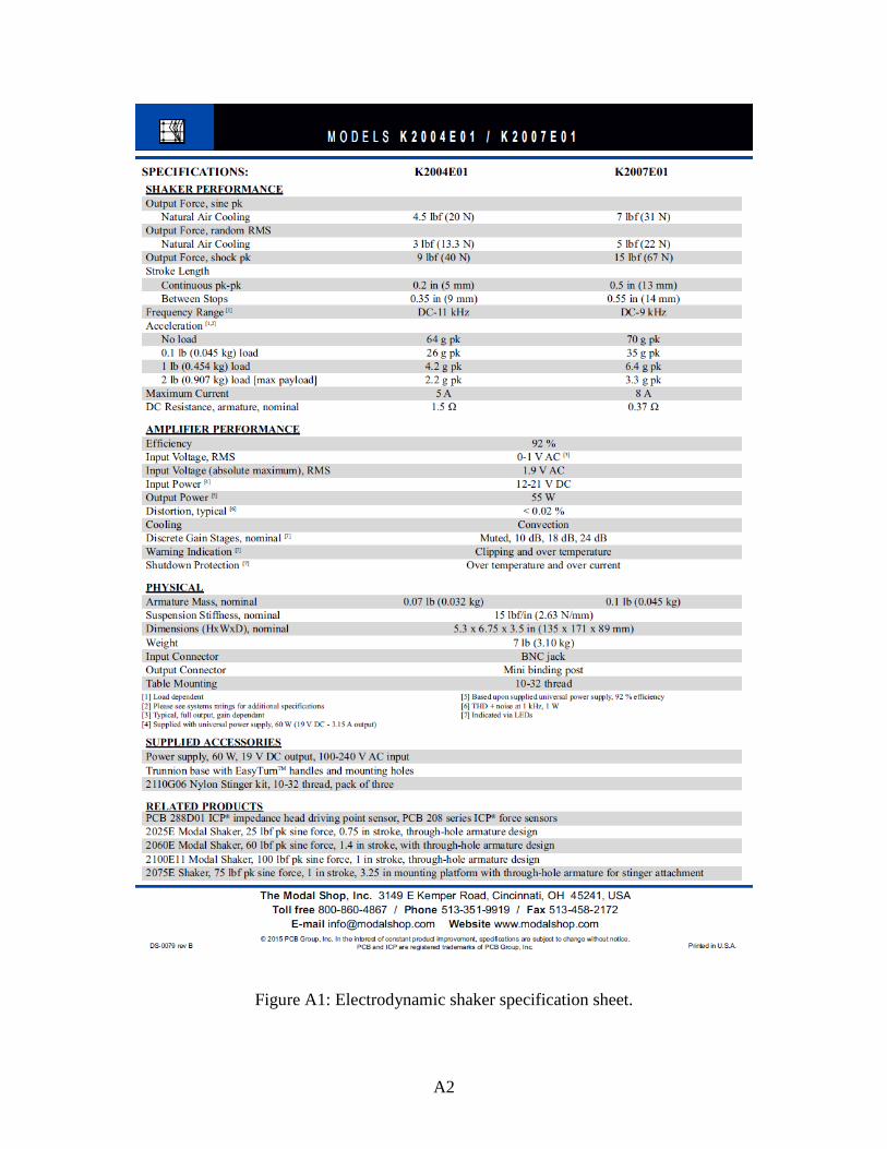
A2
Figure A1: Electrodynamic shaker specification sheet.

A3
Figure A2: Photoresistor sensor data sheet from RadioShack.

A4
Figure A3: SEM cross-section of PDMS coupon with EML phosphors [11].

A5
Figure A4: dSpace board specification sheet.

Appendix B: Chapter 3

B2
Table B1: Parameters for shaker chirp signal experiment.
Parameter Value
Offset (V) 0
Amplitude (V) 0.3
Frequency Range (Hz) 1-100
Sweep Time (sec) 500
Sampling Frequency (Hz) 100
Figure B1: Shaker chirp signal input/output.

B3
Figure B2: Pole and zero plot for fourth order shaker estimate.

B4
Figure B3: LED data sheet.

B5
Figure B4: LED wavelength response to different supply voltages.
Table B2: Parameters for LED and PR chirp signal experiment.
Parameter Value
Offset (V) 2.3
Amplitude (V) 0.1
Frequency Range (Hz) 1-100
Sweep Time (sec) 240
Sampling Frequency (Hz) 2000

B6
Figure B5: LED luminance calibration for chirp signal supply voltage range.
Figure B6: LED chirp signal input/output with LED values adjusted to luminance.

B7
Figure B7: Pole and zero plot for third order PR estimate.

Appendix C: Chapter 4

C2
Table C1: Parameters for overall system chirp signal experiment
Parameter Value
Offset (V) 0
Amplitude (V) .5
Frequency Range (Hz) 1-17.5
Sweep Time (sec) 240
Sampling Frequency (Hz) 2000
Figure C1: Overall system input/output.

Appendix D: Matlab Code

D2
Code 1: Shaker Chirp Signal Analysis Code.
T_ChirpShaker.mat
%Transfer function analysis of shaker chirp signal
%output measured by laser interferometer
%1 to 100hz over 500 sec
clc; clear all;
close all;
data1=load('Measurements/Shaker/vpp=0pt03_0pt1-100hz in 500 secs.mat');
%adjust sampling frequency due to downsampling
%convert 32int to double for math calcs
downsampling=double(data1.vpp_0pt03_0pt1_100hz_in_500_sec.Capture.Downsampling);
samplingperiod=data1.vpp_0pt03_0pt1_100hz_in_500_sec.Capture.SamplingPeriod;
Fs=1/(downsampling*samplingperiod);
%extract dSpace values
x1=data1.vpp_0pt03_0pt1_100hz_in_500_sec.Y(2).Data; %shaker (input)
y1=data1.vpp_0pt03_0pt1_100hz_in_500_sec.Y(1).Data; %laser (output)
%convert from voltage to mm
%laser interferometer sensitivity
y1=y1*.9;
time_vec1=data1.vpp_0pt03_0pt1_100hz_in_500_sec.X.Data;
%% plot input output data
%define time range to plot
tmin =0; tmax = max(time_vec1); fsize = 14;
%plot original input and output run
figure
subplot(211);
plot(time_vec1,x1,'r');
axis([tmin tmax -.02 .02]);
ylabel('Volts'); xlabel('Time (s)');
title('Shaker Input');
set(gca,'Fontsize',fsize);
grid on;grid minor;
subplot(212);
plot(time_vec1,y1);
axis([tmin tmax 0 4.5]);
ylabel('Displacement (mm)'); xlabel('Time (s)');

D3
title('Laser Output');
set(gca,'Fontsize',fsize);
grid on;grid minor;
%plot zero bias input and output run
x1zbias=x1-mean(x1);
y1zbias=y1-mean(y1);
fig1=figure;
subplot(211);
plot(time_vec1,x1zbias,'r');
axis([tmin tmax -.02 .02]);
ylabel('Volts'); xlabel('Time (s)');
title('Shaker Input');
set(gca,'Fontsize',fsize);
grid on;grid minor;
subplot(212);
plot(time_vec1,y1zbias);
axis([tmin tmax -2 2.2]);
ylabel('Displacement (mm)'); xlabel('Time (s)');
title('Laser Output');
set(gca,'Fontsize',fsize);
grid on;grid minor;
% saveas(fig1,'Measurements/Shaker/Input-Output Data ChirpShaker 1_20_16','png');
%% calculate and plot bode magnitude and phase
%calculate frequency response
fr=1:.1:100;
[Txy1 F1]=tfestimate(x1zbias,y1zbias,[],[],fr,Fs);
%calculate bode magnitude and phase
magnitude1=abs(Txy1);
gain1=20*log10(magnitude1);
phase1=atand(imag(Txy1)./real(Txy1));
%phase goes below -90 after index 198
%atand kicks it up to 90, need to adjust by -180 increments
phase1=phase1-180;
phase1(199:length(phase1))=phase1(199:length(phase1))-180;
phase1rad=phase1*pi/180;
w=F1*2*pi;
%plot bode
figure
subplot(211) %dB
semilogx(F1,gain1);
D4
% semilogx(F1,magnitude1);
axis([1 100 0 45]);
% axis([1 90 0 150]);
set(gca,'Fontsize',fsize);
ylabel('Magnitude (dB)');
% ylabel('Magnitude (mm/Volt)');
title('Shaker Frequency Response (mm/Volts)');
grid on;grid minor;
subplot(212)
semilogx(F1,phase1);
axis([1 90 -450 -100]);
set(gca,'Fontsize',fsize);
ylabel('Phase (deg)'); xlabel('Frequency (Hz)');
grid on;grid minor;
%% smooth bode plot
%use moving average to smooth out frequency response
sgain1=smooth(gain1,30);
sphase1=smooth(phase1,30);
smagnitude1=smooth(magnitude1,30);
sphase1rad=smooth(phase1rad,30);
%% Compare Frequency Response
%load System ID TF
tfest=load('Measurements/Shaker/tfshakerV2mm2_03_16.mat');
opts = bodeoptions('cstprefs');
opts.FreqUnits = 'Hz';
[m2,p2]=bode(tfest.P4Z4,w,opts);
%extract magnitude and phase values
for i=1:length(m2) %6555
mag_g2(i)=m2(1,1,i);
phase_g2(i)=p2(1,1,i);
end
%plot bode
figure
subplot(2,1,1) %dB
semilogx(F1,20*log10(mag_g2))
hold on
semilogx(F1,sgain1)
set(gca,'FontSize',fsize)
ylabel('Magnitude (dB)')

D5
title('Frequency Response (mm/Volts)')
axis([0 100 0 45])
grid on;grid minor;
hold off
%plot phase
subplot(2,1,2)
semilogx(F1,phase_g2)
hold on
semilogx(F1,sphase1)
hold off
ylabel('Phase (deg)')
xlabel('Frequency (Hz)')
legend('Approximation P4Z4','Experimental','Location','SouthWest')
axis([0 100 -440 230])
set(gca,'FontSize',fsize)
grid on;grid minor;
%% Adjusted Phase Values
% shift estimate by 180 degree increments
figure
subplot(2,1,1)
%plot magnitude (db) vs frequency (hz)
semilogx(F1,sgain1)
hold on
semilogx(F1,20*log10(mag_g2))
set(gca,'FontSize',fsize)
ylabel('Magnitude (dB)')
title('Frequency Response Adj (mm/Volts)')
axis([0 100 0 45])
grid on;grid minor;
hold off
%plot phase (degree) vs frequency (hz)
subplot(2,1,2)
semilogx(F1,sphase1)
hold on
semilogx(F1,phase_g2-360) %adjusted to compensate for arctan()
hold off
ylabel('Phase (deg)')
xlabel('Frequency (Hz)')
legend('Experimental','Approximation P4Z4','Location','SouthWest')
axis([0 100 -450 -120])
set(gca,'FontSize',fsize)
grid on;grid minor;

D6
%% PZ plot
figure
pzshaker=pzplot(tfest.P4Z4,'k');
shakerp=pole(tfest.P4Z4)
shakerz=zero(tfest.P4Z4)
set(gca,'FontSize',fsize)
title('Shaker PZ P3Z3')

D7
Code 2: LED Luminance Calibration Code
T_LED_Calibration.mat
%LED luminance calibration with LED orientation directly at spectroradiometer
%find relationship between LED voltage and luminance output
close all; clear; clc;
% Create Vled array
Vled1=[2.00:.01:2.25];
Vled2=[2.30:.05:2.50];
Vled=[Vled1 Vled2];
% Load Luminance Data
load('Measurements/Luminance Tests/lumtest2.mat')
lum=Pbright(1:31);
lumfit=lum(1:21)';
Vledfit=Vled(1:21)';
%create exponential fit
led2lumfit=fit(Vledfit,lumfit,'exp2')
% Vled vs lum
figure
plot(Vled(1:21),lum(1:21),':+') %range we are interested in
hold on
plot(led2lumfit)
title('Luminance vs LED Voltage');
xlabel('Led Voltage (V)');
ylabel('Luminance (cd/m^2)');
legend('Experimental Data','Polynomial Fit','Location','NorthWest')
axis([2 2.2 0 50]);
set(gca,'Fontsize',14);grid on;grid minor;
hold off

D8
Code 3: PR Calibration Code
T_PRCalibration.mat
%PR calibration with new 510 nm LED at different dc supply voltages
close all; clear; clc;
%% load in PR data
%(voltage drop across shunt resistor)
filename1='Measurements/Voltage Test/Voltage 2/2.0';
filename3='.mat';
for n=1:10
filename=[filename1 num2str(n-1) filename3];
load(filename); %load a data file
Vpr(n)=mean(dscapture.Y.Data);
end
filename1='Measurements/Voltage Test/Voltage 2/2.';
filename3='.mat';
for n=11:26
filename=[filename1 num2str(n-1) filename3];
load(filename); %load a data file
Vpr(n)=mean(dscapture.Y.Data);
end
for k=1:5
i=[30;35;40;45;50];
filename=[filename1 num2str(i(k)) filename3];
load(filename); %load a data file
Vpr(k+26)=mean(dscapture.Y.Data);
end
%% Create Vled array
Vled1=[2.00:.01:2.25];
Vled2=[2.30:.05:2.50];
Vled=[Vled1 Vled2];
%% Load Luminance Data
load('Measurements/Luminance Tests/lumtest2.mat')
lum=Pbright(1:31);
%last measurement was repeated, use first 31
%% Vpr vs Vled

D9
%concentrate on data less than 30 cd/m^2
% corresponds to data points 1-20
% inaccurate readings before data point 7, does not affect linear fit
figure
plot(Vled(1:20),Vpr(1:20),'-+')
% plot(Vled,Vpr)
title('Photoresistor Voltage Drop vs LED Voltage');
xlabel('LED Voltage (V)');
ylabel('PR Voltage Drop (V)');
set(gca,'FontSize',12);grid on;grid minor;
%% Vled vs lum
%Luminance calibration for LED voltages used in chirp signal calibration
lumfit=lum(21:29)';
Vledfit=Vled(21:29)';
% create exponential fit
led2lumfit=fit(Vledfit,lumfit,'exp2')
figure
% plot(Vled(21:30),lum(21:30),':+')
plot(Vled(21:29),lum(21:29),':+') %range of interest
hold on
plot(led2lumfit)
title('Luminance vs LED Voltage');
xlabel('Led Voltage (V)');
ylabel('Luminance (cd/m^2)');
legend('Experimental Data','Exponential Fit','Location','NorthWest')
axis([2.2 2.4 0 240]);
set(gca,'Fontsize',14);grid on;grid minor;
hold off
%% Vpr vs lum
figure
plot(lum(7:20),Vpr(7:20),'+')
title('PR Voltage Drop vs Luminance');
ylabel('PR Voltage Drop (V)');
xlabel('Luminance (cd/m^2)');
hold on
% create polyfit
P1=polyfit(lum(7:20),Vpr(7:20),1);

D10
vprVlumfit=polyval(P1,0:35);
plot(0:35,vprVlumfit)
legend('Data','Linear Fit','Location','BEST');
set(gca,'Fontsize',14);
grid on;grid minor;
%polyfit of inverse
P2=polyfit(Vpr(7:20),lum(7:20),1)
lumVvprfit=polyval(P2,0:.01:.3);
yfit=polyval(P2,Vpr(7:20));
%plot
figure
plot(Vpr(7:20),lum(7:20),'+')
title('Luminance vs Voltage Drop');
xlabel('PR Voltage Drop (V)');
ylabel('Luminance (cd/m^2)');
hold on
plot(0:.01:.3,lumVvprfit)
legend('Data','Linear Fit','Location','BEST');
set(gca,'Fontsize',14);
grid on;grid minor;
%% R^2 Values
%find residuals
yresid=lum(7:20)-yfit;
%square residuals
SSresid=sum(yresid.^2);
%sum of squares
SStotal=(length(yfit)-1)*var(yfit);
%find R^2
rsq=1-SSresid/SStotal
%find adjusted R^2
req_adj=1-SSresid/SStotal*(length(yfit)-1)/(length(yfit)-length(P2))
%% LED Wavelength
%LED wavelength dependence on supply voltage/current
%plot
figure
plot(Vled(1:20),Peakw(1:20),':+k')

D11
axis([2 2.19 519 525])
xlabel('LED Circuit Voltage (V)');
ylabel('Peak Wavelength (nm)');
title('LED Wavelength Variation')
set(gca,'FontSize',12);grid on;grid minor;
%% 3-D plot
Vpr_t=linspace(0,.3,1000);
d_t=linspace(5,25,1000);
for i=1:1000
for j=1:1000
L_t(i,j)=126.997*((Vpr_t(i))-.03417*(15-d_t(j)))+.5631;
end
end
figure
h=surf(d_t,Vpr_t,L_t)
set(h,'LineStyle','none')
axis([5 25 0 .3 0 40])
title('PR Voltage Static Luminance Calibration')
xlabel('Distance (mm)')
ylabel('PR Circuit Voltage (V)');
zlabel('Luminance (cd/m^2)');
set(gca,'FontSize',12);grid on;grid minor;

D12
Code 4: PR Distance Calibration Code.
T_PRDistanceTest.mat
%Dependence of PR voltage drop vs distance from light source
clc; clear all;
close all;
%load in measurement files
data1=load('Measurements/d1.mat');
data2=load('Measurements/d2.mat');
data3=load('Measurements/d3.mat');
data4=load('Measurements/d4.mat');
data5=load('Measurements/d5.mat');
data6=load('Measurements/d6.mat');
data7=load('Measurements/d7.mat');
%save average data
v1=mean(data1.d1.Y.Data);
v2=mean(data2.d2.Y.Data);
v3=mean(data3.d3.Y.Data);
v4=mean(data4.d4.Y.Data);
v5=mean(data5.d5.Y.Data);
v6=mean(data6.d6.Y.Data);
v7=mean(data7.d7.Y.Data);
%concatenate into array
%adjust 6 and 7
v=[v1 v6 v2 v7 v3 v4 v5];
%create distance array
distances=[4.92
7.21
9.59
12.39
14.22
19.93
24.66];
%plot distance vs voltage drop
figure
plot(distances, v,'-+')
title('Voltage Drop vs Distance');
xlabel('Distance (mm)');
ylabel('Voltage Drop (mm)');
set(gca,'FontSize',12);grid on;grid minor;

D13
%find linear fit
%f(x)=-.03417*x+4.592
d=4.92:.1:24.66; %distance range (mm)
%determine fitted values
fitvalues=-.03417*d+4.592;
%plot relationship
figure
plot(distances, v,'-+')
hold on
plot(d,fitvalues)
axis([4 26 3.7 4.5])
title('Voltage Drop vs Distance');
xlabel('Distance (mm)');
ylabel('Voltage Drop (V)');
set(gca,'FontSize',12);grid on;grid minor;
legend('Experimental Data','Linear Fit')
hold off

D14
Code 5: LED Chirp Signal Analysis
T_ChripAnalysisPR.mat
%Frequency analysis of led chirp signal
%Led head on with PR at 15 mm distance
%.01 to 100hz over 240 sec
%2.3 v offset with .1v amplitude
clc; clear all;
close all;
%% Load measurement data
data1=load('Measurements/Chirp/chirp1.6.16.mat');
%adjust sampling frequency due to downsampling
%convert 32int to double for math calcs
downsampling=double(data1.chirp1_6_16.Capture.Downsampling);
samplingperiod=data1.chirp1_6_16.Capture.SamplingPeriod;
Fs=1/(downsampling*samplingperiod);
%extract dSpace values
x1=data1.chirp1_6_16.Y(1).Data; %led out (input)
y1=data1.chirp1_6_16.Y(2).Data; %pr voltage drop in (output)
time_vec1=data1.chirp1_6_16.X.Data;
%% Plot input(VLED) output(VPR) data
%define time range to plot
tmin =0; tmax = max(time_vec1); fsize = 14;
%plot original input and output run
figure
subplot(211);
plot(time_vec1,x1,'r');
axis([tmin tmax 2 3]);
ylabel('Volts'); xlabel('Time (s)');
title('LED Input');
set(gca,'Fontsize',fsize);
grid on;grid minor;
subplot(212);
plot(time_vec1,y1);
axis([tmin tmax .5 3.5]);
ylabel('Volts'); xlabel('Time (s)');
title('Photoresistor Output (V)');

D15
set(gca,'Fontsize',fsize);
grid on;grid minor;
%% Plot input(lumLED) output(VPR) data
%load luminance conversion
lumfit=load('led2lumfit_chirp.mat');
lum=lumfit.led2lumfit(x1)';
%plot original input and luminance output
figure
subplot(211);
plot(time_vec1,lum,'r');
axis([tmin tmax 20 250]);
ylabel('Luminance (cd/m^2)'); xlabel('Time (s)');
title('LED Input');
set(gca,'Fontsize',fsize);
grid on;grid minor;
subplot(212);
plot(time_vec1,y1);
axis([tmin tmax .5 3.5]);
ylabel('Volts'); xlabel('Time (s)');
title('Photoresistor Output (V)');
set(gca,'Fontsize',fsize);
grid on;grid minor;
%plot zero bias input and luminance output
lumzbias=lum-mean(lum);
y1zbias=y1-mean(y1); %PR circuit voltage drop
subplot(211);
plot(time_vec1,lumzbias,'r');
axis([tmin tmax -125 100]);
ylabel('Luminance (cd/m^2)'); xlabel('Time (s)');
title('LED Input');
set(gca,'Fontsize',fsize);
grid on;grid minor;
subplot(212);
plot(time_vec1,y1zbias);
axis([tmin tmax -2 1.5]);
ylabel('Volts'); xlabel('Time (s)');
title('Photoresistor Output (V)');
set(gca,'Fontsize',fsize);
grid on;grid minor;

D16
%% Calculate and plot bode magnitude and phase
%calculate experimental frequency response
fr=1:.01:100;
[Txy1 F1]=tfestimate(lumzbias,y1zbias,[],[],fr,Fs);
%calculate bode magnitude and phase
magnitude1=abs(Txy1); %absolute value
gain1=20*log10(magnitude1); %dB
phase1=atand(imag(Txy1)./real(Txy1));
phase1rad=atan(imag(Txy1)./real(Txy1));
w=F1*2*pi;
figure;
subplot(211) %dB
semilogx(F1,gain1);
% semilogx(F1,magnitude1);
axis([1 100 -60 -30]);
set(gca,'Fontsize',fsize);
title('Frequency Response (Vpr/Lum)')
ylabel('Magnitude (dB)');
grid on;grid minor;
subplot(212)
semilogx(F1,phase1);
axis([1 90 -90 90]);
set(gca,'Fontsize',fsize);
ylabel('Phase (deg)'); xlabel('Frequency (Hz)');
grid on;grid minor;
%% smooth values
%use a 30 point moving average to smooth the data
sgain1=smooth(gain1,30);
sphase1=smooth(phase1,30);
smagnitude1=smooth(magnitude1,30);
sphase1rad=smooth(phase1rad,30);
figure
subplot(211) %dB
semilogx(F1,sgain1);
% semilogx(F1,smagnitude1);
axis([1 90 -50 -35]);

D17
set(gca,'Fontsize',fsize);
ylabel('Magnitude (dB)');
title('Frequency Response (Vpr/Lum)')
grid on;grid minor;
subplot(212)
semilogx(F1,sphase1);
axis([1 90 -90 0]);
set(gca,'Fontsize',fsize);
ylabel('Phase (deg)');
xlabel('Frequency (Hz)');
grid on;grid minor;
%% P3Z3 estimate
% compare experimental values to tf found in system id
tf=load('tfP3Z3lum.mat'); %three poles and three 3 zeros estimation
%bode plot of estimated tf
opts = bodeoptions('cstprefs');
opts.FreqUnits = 'Hz'; %change bode plot to Hz
w2=1:1:100*2*pi; %define frequency range
f2=w2/2/pi;
%extract magnitude and phase values to display on same bode plot
[m2,p2]=bode(tf.P3Z3,w2,opts);
for i=1:628
mag_g2(i)=m2(1,1,i);
phase_g2(i)=p2(1,1,i);
end
%plot bode
figure
subplot(2,1,1)
semilogx(f2,20*log10(mag_g2),'r')
hold on
semilogx(F1,sgain1)
title('Frequency Response (Vpr/Lum)');
ylabel('Magnitude (dB)');
legend('TF Estimate P3Z3','Exp Data','Location','SouthWest');
set(gca,'FontSize',12);grid on;grid minor;
axis([1 100 -55 -35])
hold off
subplot(2,1,2)
semilogx(f2,phase_g2,'r')

D18
hold on
semilogx(F1,sphase1)
ylabel('Phase (deg)');
xlabel('Frequency (Hz)');
set(gca,'FontSize',12);grid on;grid minor;
axis([1 100 -90 0])
hold off
%% System ID P1Z0
%plot P1Z0 tf found from system ID
tf3=load('tfP1Z0lum.mat'); %one ploe estimation
%extract magnitude and phase values to display on same bode plot
[m3,p3]=bode(tf3.P1Z0,w2,opts);
for i=1:628
mag_g3(i)=m3(1,1,i);
phase_g3(i)=p3(1,1,i);
end
%plot bode
figure
subplot(2,1,1)
semilogx(f2,20*log10(mag_g3),'r')
hold on
semilogx(F1,sgain1)
title('Frequency Response (Vpr/Lum)');
ylabel('Magnitude (dB)');
legend('TF Estimate P1Z0','Exp Data','Location','SouthWest');
set(gca,'FontSize',12);grid on;grid minor;
axis([1 100 -55 -35])
hold off
subplot(2,1,2)
semilogx(f2,phase_g3,'r')
set(gca,'FontSize',12);grid on;grid minor;
hold on
semilogx(F1,sphase1)
ylabel('Phase (deg)');
xlabel('Frequency (Hz)');
axis([1 100 -90 0])
hold off
D19
%% Pole and Zeros
%one ploe system
polep1z0=pole(tf3.P1Z0);
zerop1z0=zero(tf3.P1Z0);
%plot pz diagram
figure
pzPRp1z0=pzplot(tf3.P1Z0,'k');
title('PR PZ P1Z0')
set(gca,'FontSize',12)
%P3Z3
polep3z3=pole(tf.P3Z3);
zerop3z3=zero(tf.P3Z3);
%plot pz diagram
figure
pzPRp3z3=pzplot(tf.P3Z3,'k');
title('PR PZ P3Z3')
set(gca,'FontSize',12)

D20
Code 6: Numerical Method for Temporal Luminance Response
T_DifferentialTemporalAnalysis.mat
%Use differential form to determine temporal luminance response
%analyzing one case of .5V shaker voltage at 10 Hz
close all; clear; clc;
%load in a PR voltage file 10Hz
load('Measurements\ML Frequency 1_14_16\1.10.mat')
t=dscapture.X.Data; %load time data
Vs=dscapture.Y(1).Data; %load in shaker input signal
Vpr=dscapture.Y(2).Data; %load in PR voltage measurement
%% Calibration
%use dynamic calibration
sVpr=smooth(Vpr,5); %smooth PR voltage data
vpr=diff(sVpr)/(1/2000); %derivative of smooth PR voltage data
L=(1/1.8228)*(vpr+188.5*sVpr(1:length(vpr)));
sL=smooth(L,5); %smooth luminance data
%plot temporal response
figure;
plot(t(1:length(sL)),sL,'k')
axis([0 .2 16 39])
title('Luminance Values')
xlabel('Time (s)')
ylabel('Luminance (cd/m^2)')
set(gca,'FontSize',12);grid on;grid minor;
figure;
plot(t(1:length(sVpr)),sVpr,'k')
axis([0 .2 .16 .32])
title('Photoresistor Circuit Values')
xlabel('Time (s)')
ylabel('PR Circuit (V)')
set(gca,'FontSize',12);grid on;grid minor;
%plot normalized figure
figure
plot(t,.5+.5*Vs/max(Vs)) %shift to center
hold on
plot(t,sVpr/max(sVpr),'r')

D21
plot(t(1:length(sL)),sL/max(sL),'k')
hold off
axis([0 .2 0 1])
set(gca,'FontSize',12);grid on;grid minor;
title('Normalized Response')
xlabel('Time (s)');
ylabel('Normalized Value')
legend('Shaker Input Voltage','PR Voltage Response','Luminance Response'...
,'Location','SouthEast')

D22
Code 7: EML Chirp Signal Analysis of Overall System
T_ChripML.mat
%Frequency analysis of entire system
%ML coupon excited by electromechanical shaker
%1 to 17.5 Hz at .5V amplitude
clc; clear all;
close all;
%load measurement data
data1=load('Measurements/ML Chirp 1_7_16/mlchirp1_7_16.mat');
%adjust sampling frequency due to downsampling
%convert 32int to double for math calcs
downsampling=double(data1.mlchirp1_7_16.Capture.Downsampling);
samplingperiod=data1.mlchirp1_7_16.Capture.SamplingPeriod;
Fs=1/(downsampling*samplingperiod);
%extract dSpace values
x1=data1.mlchirp1_7_16.Y(1).Data; %shaker out (input)
y1=data1.mlchirp1_7_16.Y(2).Data; %pr voltage drop (output)
time_vec1=data1.mlchirp1_7_16.X.Data;
%% plot input output data
%define time range to plot
tmin =0; tmax = max(time_vec1); fsize = 14;
%plot original input and output run
figure
subplot(211);
plot(time_vec1,x1,'r');
axis([tmin tmax -1 1]);
ylabel('Voltage');
title('Shaker Input');
set(gca,'Fontsize',fsize);
grid on;grid minor;
subplot(212);
% plot(time_vec1,lum);
plot(time_vec1,y1);
axis([tmin tmax 0 .6]);
ylabel('Voltage'); xlabel('time (s)');
title('Photoresistor Output');

D23
set(gca,'Fontsize',fsize);
grid on;grid minor;
%% calculate and plot bode magnitude and phase
%calculate experimental frequency response
fr=1:.01:100;
[Txlum F1]=tfestimate(x1,y1,[],[],fr,Fs);
%calculate bode magnitude and phase
magnitudeML1=abs(Txlum);
gainML1=20*log10(magnitudeML1);
phaseML1=atand(imag(Txlum)./real(Txlum));
phaseML1rad=atan(imag(Txlum)./real(Txlum));
w=F1*2*pi;
fig2=figure;
subplot(211) %gain
plot(F1,gainML1);
% plot(F1,magnitudeML1);
axis([1 15 -60 -10]);
% axis([1 15 0 .12]);
set(gca,'Fontsize',fsize);
ylabel('Magnitude (dB)');
% ylabel('Magnitude (Vpr/V_S)');
title('System Frequency Response (Vpr/V_S)')
grid on;grid minor;
subplot(212)
plot(F1,phaseML1);
axis([1 15 -100 100]);
set(gca,'Fontsize',fsize);
ylabel('Phase (deg)'); xlabel('Frequency (Hz)');
grid on;grid minor;

D24
Code 8: Experimental Analysis of EML Coupon’s Frequency Response
MagandPhase.mat
close all; clear; clc;
%Load in experimental magnitude, gain, and phase data
%magnitude values are in absolute
%gain values are in dB
%phase values are in deg
F1ML=load('F1ML.mat');
F1Shaker=load('F1Shaker.mat');
gainML1=load('gainML1.mat');
magML1=load('magML1.mat');
phaseML1=load('phaseML1.mat');
gainPR1s=load('gainPR1s.mat');
magPR1s=load('magPR1s.mat');
phasePR1s=load('phasePR1s.mat');
gainShaker1=load('gainShaker1.mat');
magShaker1=load('magShaker1.mat');
phaseShaker1=load('phaseShaker1.mat');
%extract variables from structs
F1=F1ML.F1;
F1Shaker=F1Shaker.F1;
gainML=gainML1.gainML1;
magML=magML1.magnitudeML1;
phaseML=phaseML1.phaseML1;
gainPRs=gainPR1s.sgain1';
magPRs=magPR1s.smagnitude1';
phasePRs=phasePR1s.sphase1';
gainShaker=gainShaker1.gain1;
magShaker=magShaker1.magnitude1;
phaseShaker=phaseShaker1.phase1;
%inverse of tf is same as negative gain or phase
%%%%cant do this right away, not the same size matrices because sampling
%%%%rate for shaker calibration was much lower (200 vs 2000)
%shaker is also over a longer time period (500 sec vs 240 sec)
% only use every 9901/991 (~10) point to reduce vectors to same size
j=1;
for i=1:10:9901
gainML2(j)=gainML(i);
magML2(j)=magML(i);

D25
phaseML2(j)=phaseML(i);
gainPR2(j)=gainPRs(i);
magPR2(j)=magPRs(i);
phasePR2(j)=phasePRs(i);
j=j+1;
end
%% Mag and Phase Calcs
%Find magnitude, gain, and phase values for the ML coupon
gain=-gainPR2+gainML2-gainShaker;
magnitude=(1./magPR2).*magML2.*(1./magShaker);
phase=-phasePR2+phaseML2-phaseShaker;
%adjust phase by 180 deg
phase=phase-180;
%% Plot
%plot ML coupon frequency response dB
dB=gain;
figure
subplot(2,1,1)
plot(F1Shaker(1:166),dB(1:166))
axis([1 17.5 -55 -10])
set(gca,'Fontsize',14);
grid on; grid minor;
title('ML Coupon Frequency Response (L/\delta)')
ylabel('Magnitude (dB)');
subplot(2,1,2)
plot(F1Shaker(1:166),phase(1:166))
axis([1 17.5 -100 20])
set(gca,'Fontsize',14);
grid on; grid minor;
ylabel('Phase (deg)');
xlabel('Frequency (Hz)');
%plot ML coupon frequency response absolute magnitude
absmag=magnitude;
figure
subplot(2,1,1)
plot(F1Shaker(1:166),absmag(1:166))
axis([1 15 0 .12])
set(gca,'Fontsize',14);
grid on; grid minor;

D26
title('ML Coupon Frequency Response (L/\delta)')
ylabel('Magnitude (L/\delta)');
subplot(2,1,2)
plot(F1Shaker(1:166),phase(1:166))
axis([1 15 -100 20])
set(gca,'Fontsize',14);
grid on; grid minor;
ylabel('Phase (deg)');
xlabel('Frequency (Hz)');


![Carbon Nanotubes and Semiconducting Polymer Nanocomposites · 2018-09-25 · Carbon Nanotubes and Semiconduc ting Polymer Nanocomposites 471 ion mass transfer [28]. In some host polymers,](https://static.fdocuments.in/doc/165x107/5f42727e6bc30357fd01dba3/carbon-nanotubes-and-semiconducting-polymer-nanocomposites-2018-09-25-carbon-nanotubes.jpg)


![Polymer blends • molecular level • A short Review on new ......hydrogen bonding, acid-base reaction or charge transfer [4]. Classifications of polymer blends [5-7] During the last](https://static.fdocuments.in/doc/165x107/6132500fdfd10f4dd73a5e43/polymer-blends-a-molecular-level-a-a-short-review-on-new-hydrogen-bonding.jpg)


