TRANSACTION ON SMART GRID 1

Reinforcement Learning Applied to an ElectricWater Heater: From Theory to Practice

F. Ruelens, B. J. Claessens, S. Quaiyum, B. De Schutter, R. Babuska, and R. Belmans

Abstract—Electric water heaters have the ability to storeenergy in their water buffer without impacting the comfort ofthe end user. This feature makes them a prime candidate forresidential demand response. However, the stochastic and non-linear dynamics of electric water heaters, makes it challenging toharness their flexibility. Driven by this challenge, this paper for-mulates the underlying sequential decision-making problem as aMarkov decision process and uses techniques from reinforcementlearning. Specifically, we apply an auto-encoder network to finda compact feature representation of the sensor measurements,which helps to mitigate the curse of dimensionality. A well-known batch reinforcement learning technique, fitted Q-iteration,is used to find a control policy, given this feature representation.In a simulation-based experiment using an electric water heaterwith 50 temperature sensors, the proposed method was able toachieve good policies much faster than when using the full stateinformation. In a lab experiment, we apply fitted Q-iteration toan electric water heater with eight temperature sensors. Furtherreducing the state vector did not improve the results of fittedQ-iteration. The results of the lab experiment, spanning 40 days,indicate that compared to a thermostat controller, the presentedapproach was able to reduce the total cost of energy consumptionof the electric water heater by 15%.

Index Terms—Auto-encoder network, demand response, elec-tric water heater, fitted Q-iteration, reinforcement learning.

I. INTRODUCTION

THE share of renewable energy sources is expected toreach 25% of the global power generation portfolio by

2020 [1]. The intermittent and stochastic nature of mostrenewable energy sources, however, makes it challenging tointegrate these sources into the power grid. Successful inte-gration of these sources requires flexibility on the demandside through demand response programs. Demand responseprograms enable end users with flexible loads to adapt theirconsumption profile in response to an external signal. Aprominent example of flexible loads are electric water heaterswith a hot water storage tank [2], [3]. These loads have theability to store energy in their water buffer without impactingthe comfort level of the end user. In addition to havingsignificant flexibility, electric water heaters can consume about2 MWh per year for a household with a daily hot waterdemand of 100 liters [4]. As a result, electric water heaters area prime candidate for residential demand response programs.

F. Ruelens and R. Belmans are with the Department of Electrical Engineer-ing, KU Leuven/EnergyVille, Belgium (frederik.ruelens@esat.kuleuven.be).

B. J. Claessens is with the Energy Department of Vito/EnergyVille, Belgium(bert.claessens@vito.be).

S. Quaiyum is with the Department of Electrical Engineering, UppsalaUniversity, Sweden.

B. De Schutter and R. Babuska are with the Delft Center for Systems andControl, Delft University of Technology, The Netherlands.

Previously, the flexibility offered by electric water heaters hasbeen used for frequency control [5], local voltage control [6],and energy arbitrage [7], [8]. Amongst others, two prominentcontrol paradigms in the demand response literature on electricwater heaters are model-based approaches and reinforcementlearning.

Perhaps the most researched control paradigm applied todemand response are model-based approaches, such as ModelPredictive Control (MPC) [7], [9], [8]. Most MPC strategiesuse a gray-box model, based on general expert knowledgeof the underlying system dynamics, requiring a system iden-tification step. Given this mathematical model, an optimalcontrol action can be found by solving a receding horizonproblem [10]. In general, the implementation of MPC consistsof several critical steps, namely, selecting accurate models,estimating the model parameters, estimating the state of thesystem, and forecasting of the exogenous variables. All thesesteps make MPC an expensive technique, the cost of whichneeds to be balanced out by the possible financial gains [11].Moreover, possible model errors resulting from an inaccuratemodel or forecast, can effect the stability of the MPC con-troller [12], [13].

In contrast to MPC, Reinforcement Learning (RL) tech-niques [14] do not require expert knowledge and consider theirenvironment as a black-box. RL techniques enable an agentto learn a control policy by interacting with its environment,without the need to use modeling and system identificationtechniques. In [15], Ernst et al. state that the trade-off in apply-ing MPC and RL mainly depends on the quality of the expertknowledge about the system dynamics that could be exploitedin the context of system identification. In most residentialdemand response applications, however, expert knowledgeabout the system dynamics or future disturbances might beunavailable or might be too expensive to obtain relative to theexpected financial gain. In this context, RL techniques are anexcellent candidate to build a general purpose agent that canbe applied to any demand response application.

This paper proposes a learning agent that minimizes thecost of energy consumption of an electric water heater. Theagent measures the state of its environment through a setof sensors that are connected along the water buffer of theelectric water heater. However, learning in a high-dimensionstate space can significantly impact the learning rate of the RLalgorithm. This is known as the “curse of dimensionality”.A popular approach to mitigate its effects is to reduce thedimensionality of the state space during a pre-processing step.Inspired by the work of [16], this paper applies an auto-encoder network to reduce the dimensionality of the state

arX

iv:1

512.

0040

8v1

[cs

.LG

] 2

9 N

ov 2

015

TRANSACTION ON SMART GRID 2

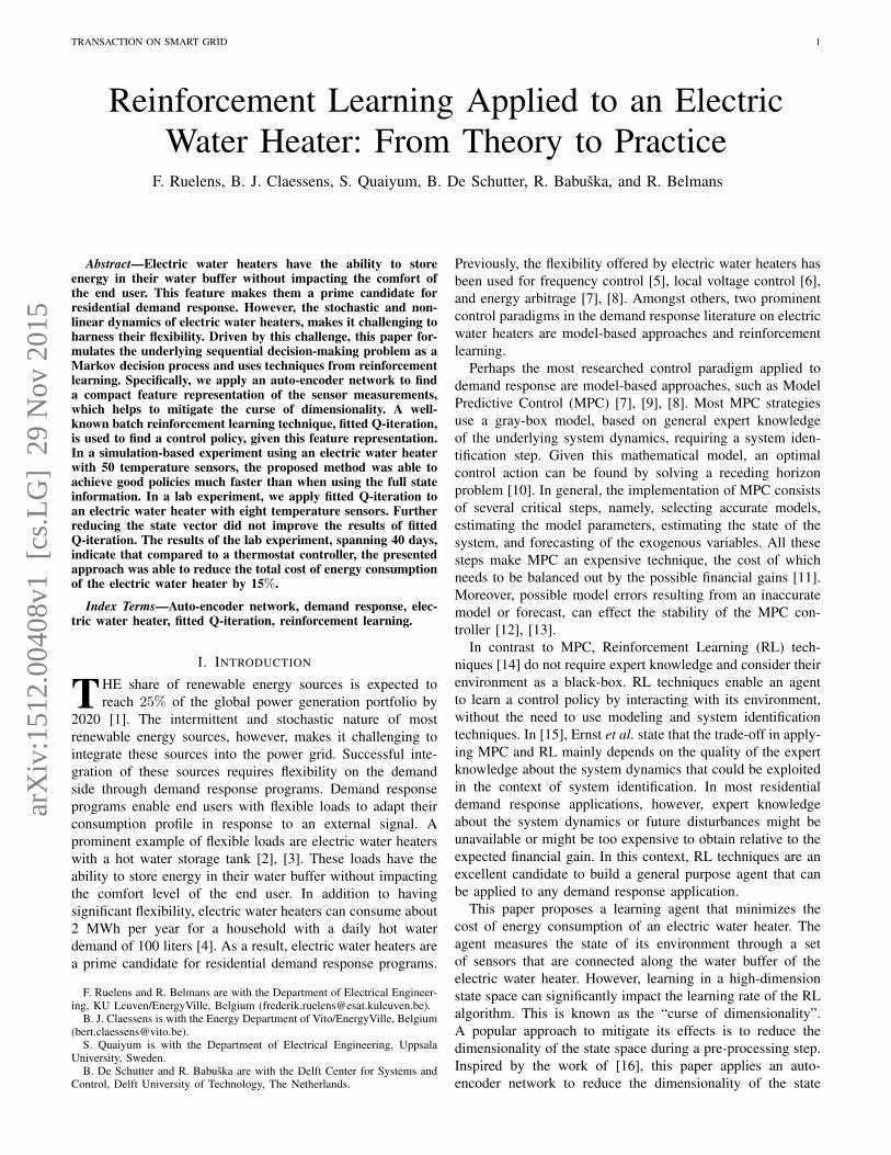
vector. By so doing, this paper makes following contributions:(1) we demonstrate how a well-established RL technique, fittedQ-iteration, can be combined with an auto-encoder network tominimize the cost of energy consumption of an electric waterheater; (2) in a simulation-based experiment, we assess theperformance of different state representations and batch sizes;(3) we successfully apply an RL agent to an electric waterheater in the lab (Fig. 1).

The remainder of this paper is organized as follows. Sec-tion II gives a non-exhaustive literature overview of RL relatedto demand response. Section III maps the considered demandresponse problem to a Markov decision process. Section IVdescribes how an auto-encoder network can be used to finda low-dimensional state representation, followed by a descrip-tion of the fitted Q-iteration algorithm in Section V. Section VIpresents the results of the simulation-based experiments andSection VII presents the results of the lab experiment. Finally,Section VIII draws conclusions and discusses future work.

II. REINFORCEMENT LEARNING

This section gives a non-exhaustive overview of recentdevelopments related to Reinforcement Learning (RL) anddemand response. Perhaps the most widely used model-freeRL technique applied to a demand response setting is stan-dard Q-learning [17], [18], [19], [20]. After each interactionwith the environment, Q-learning uses temporal differencelearning [14] to update its state-action value function or Q-function. A major drawback of Q-learning is that the givenobservation is discarded after each update. As a result, moreinteractions are needed to spread already known informationthrough the state space. This inefficient use of informationlimits the application of Q-learning to real-world applications.

In contrast to Q-learning, batch RL techniques [21], [22],[23] are more data efficient, since they store and reuse pastinteractions. As a result, batch RL techniques require lessinteractions with their environment, which makes them morepractical for real-world applications, such as demand response.Perhaps the most popular batch RL technique which has beenapplied to a wide range of applications [16], [24], [25] is fittedQ-iteration developed by Ernst et al. [21]. Fitted Q-iterationiteratively estimates the Q-function given a fixed batch of pastinteractions. An online version that uses a neural network,neural fitted Q-iteration, has been proposed by Riedmiller etal. in [22]. Finally, an interesting alternative is to combineexperience replay to an incremental RL technique such as Q-learning or SARSA [26]. In [27], the authors demonstrate howfitted Q-iteration can be used to control a cluster of electricwater heaters. The results indicate that fitted Q-iteration wasable to reduce the cost of energy consumption of a cluster of100 electric water heaters after a learning period of 40 days.In addition, [28] shows how fitted Q-iteration can be extendedto reduce the cost of energy consumption of a heat-pumpthermostat given that a forecast of the outside temperature isprovided.

A promising alternative to the previously mentioned model-free techniques are model-based or model-assisted RL tech-niques. For example, the authors of [29] present a model-based

Fig. 1. Setup of the electric water heater used during the lab experiment.Eight temperature sensors were placed under the insulation material of thebuffer tank.

policy search method that learns a Gaussian process to modeluncertainties. In addition, inspired by [30], the authors of [31]demonstrate how a model-assisted batch RL technique can beapplied to control a building heating system.

III. PROBLEM FORMULATION

The aim of this work is to develop a controller or agentthat minimizes the cost of energy consumption of an electricwater heater, given an external price profile. This price profileis provided to the agent at the start of each day. The agentcan measure the temperature of the water buffer through aset of temperature sensors that are connected along the hullof the buffer tank. Following the approach presented in [28],the electric water heater is equipped with a backup controllerthat overrules the control action from the agent when thesafety or comfort constraints of the end user are violated. Achallenge in developing such an agent is that the dynamics ofthe electric water heater, the future hot water demand and thesettings of the backup controller are unknown to the agent. Toovercome this challenge, this paper leverages on the previouswork of [16], [21], [28] and applies techniques from RL.

A. Markov decision process framework

To apply RL, this paper formulates the underlying se-quential decision-making problem of the learning agent as aMarkov decision process formulation. The Markov decisionprocess formulation is defined by its d-dimensional state spaceX ⊂ Rd, its action space U ⊂ R, its stochastic discrete-timetransition function f , and its cost function ρ. The optimizationhorizon is considered finite, comprising T ∈ N \ 0 steps,where at each discrete time step k, the state evolves following:

xk+1 = f(xk, uk,wk) ∀k ∈ 1, ..., T − 1, (1)

where a random disturbance wk is drawn from a conditionaldistribution pW(·|xk), uk ∈ U is the control action and xk ∈X the state. Associated with each state transition, a cost ck isgiven by:

ck = ρ(xk, uk,wk) ∀k ∈ 1, ..., T. (2)

TRANSACTION ON SMART GRID 3

The goal of the learning agent is to find an optimal controlpolicy h∗ : X → U that minimizes the expected T -stagereturn for any state in the state space. The expected T -stagereturn JhT starting from x1 and following a policy h is definedas follows:

JhT (x1) = EpW(·|xk)

[T∑k=1

ρ(xk, h(xk),wk)

], (3)

where E denotes the expectation operator over all possiblestochastic realizations.

A more convenient way to characterize a policy is by usinga state-action value function or Q-function:

Qh(x, u) = EpW(·|x)

[ρ(x, u,w) + JhT (f(x, h(x),w))

], (4)

which indicates the cumulative return starting from state x andby taking action u and following h thereafter.

The optimal Q-function corresponds the best Q-function thatcan be obtained by any policy:

Q∗(x, u) = minhQh(x, u). (5)

Starting from an optimal Q-function for every state-action pair,the optimal policy h∗ is calculated as follows:

h∗(x) ∈ arg minu∈U

Q∗(x, u), (6)

where Q∗ satisfies the Bellman optimality equation [32]:

Q∗(x, u) = Ew∼pW(·|x)

[ρ(x, u,w) + min

u′∈UQ∗(f(x, u,w), u′)

].

(7)

Following the notation introduced in [28], the next threeparagraphs give a description of the state, the action, and thecost function tailored to an electric water heater.

B. Observable state vector

The observable state vector of an electric water heater con-tains a time-related component and a controllable component.The time-related component xt describes the part of the staterelated to timing, which is relevant for the dynamics of thesystem. Specifically, the tap water demand of the end user isconsidered to have diurnal and weekly patterns. As such, thetime-related component contains the day of the week and thequarter in the day. The controllable component xph representsphysical state information that is measured locally and isinfluenced by the control action. The controllable componentcontains the temperature measurements of the ns sensorsthat are connected along the hull of the storage tank. Theobservable state vector is given by:

xk = ( d, t︸︷︷︸xt

k

, T 1k , . . . , T

ik, . . . , T

ns

k︸ ︷︷ ︸xph

k

), (8)

where d ∈ 1, . . . , 7 is the current day of the week,t ∈ 1, . . . , 96 is the quarter in the day and T ik denotes thetemperature measurements of sensor i at time step k.

C. Control action

The learning agent can control the heating element of theelectric water heater with a binary control action uk ∈ 0, 1,where 0 indicates off and 1 on. However, the backup mecha-nism, which enacts the comfort and safety constraints of theend user, can overrule this control action of the learning agent.The function B : X × U → Uph maps the control actionuk ∈ U to a physical action uphk ∈ Uph according to:

uphk = B(xk, uk,θ), (9)

where the vector θ defines the safety and user-defined comfortsettings of the backup controller. In order to have a genericapproach we assume that the logic of the backup controller isunknown to the learning agent. However, the learning agentcan measure the physical action uphk enforced by the backupcontroller (see Fig. 2), which is required to calculate the cost.

The logic of the backup controller of the electric waterheater is defined as:

B(x, u,θ) =

P e if xsoc(x,θ) ≤ xsoc(θ)uP e if xsoc(θ) < xsoc(x,θ) < xsoc(θ),

0 if xsoc(x,θ) ≥ xsoc(θ)(10)

where P e is the electrical power rating of the heating element,xsoc(x,θ) is the current state of charge and xsoc(θ) andxsoc(θ) are the upper and lower bounds for the state of charge.A detailed description of how the state of charge is calculatedcan by found in [3].

D. Cost function

At the start of each optimization period T∆t, the learningagent receives a price vector λ = λkTk=1 for the next T timesteps. At each time step, the agent receives a cost ck accordingto:

ck = uphk λk∆t, (11)

where λk is the electricity price during time step k, and ∆tthe length of one control period.

IV. BATCH OF FOUR-TUPLES

Generally, batch RL techniques estimate the Q-functionbased on a batch of four-tuples (xl, ul,x

′l, cl). This paper,

however, considers the following batch of four-tuples:

F = (xl, ul,x′l, uphl ), l = 1, . . . ,#F, (12)

where for each l, the next state x′l, and the physical action uphlhave been obtained as a result of taking control action ul inthe state xl. Note that, F does not include the observed costcl, since the cost depends on the price vector that is providedto the learning agent at the start of each day.

As defined by (8), xl contains all temperature measurementsof the sensors connected to the hull of the water buffer.Learning in a high-dimensional state space requires moreobservations from the environment to estimate the Q-function,as more tuples are needed to cover the state-action space.This is known as the “curse of dimensionality”. This cursebecomes even more pronounced in practical applications,

TRANSACTION ON SMART GRID 4

Algorithm 1 Fitted Q-iteration [21] using feature vectors.

Require: R =

(zl, ul, z′l, u

phl ), l = 1, . . . ,#R

, λtTt=1

1: initialize Q0 to zero2: for N = 1, . . . , T do3: for l = 1, . . . ,#R do4: cl ← uphl λt B where t is to the quarter in the day of

the time-related component xtl = (d, t) of state zl

5: QN,l ← cl + minu∈U

QN−1(z′l, u)

6: end for7: use a regression technique to obtain QN fromTreg =

((zl, ul) , QN,l

), l = 1, . . . ,#R

.

8: end forEnsure: Q∗ = QT

where each observation corresponds to a “real” interation withthe environment.

A pre-processing step can be used to find a compact andmore efficient representation of the state space and can help toconverge to a good policy much faster [33]. A popular tech-nique to find a compact representation is to use a handcraftedfeature vector based on insights of the considered controlproblem [34]. Alternative approaches that do not require priorknowledge are unsupervised feature learning algorithms, suchas auto-encoders [16] or a principal component analysis [33].

As illustrated in Fig. 2, this paper demonstrates how anauto-encoder can be used to find a compact representation ofthe sensory input data. An auto-encoder network is a neuralnetwork that maps its output back to its input. By selecting alower number of neurons in the middle hidden layer than inthe input layer p < d, the auto-encoder can be used to reducethe dimensionality of the input data.

The reduced feature vector zl ∈ Z ⊂ Rp can be calculatedas follows:

zl = (xtl,Φenc(x

phl ,w, b)), (13)

where w and b denote the weights and the biases that connectthe input layer with the middle hidden layer of the auto-encoder network. The function Φenc : X → Z is an encoderfunction and maps the observed state vector xl to the featurevector zl. To train the weights of the auto-encoder, a conjugategradient descent algorithm is used as presented in [35].

In the next section, fitted Q-iteration is used to find a policyh : Z → U that maps every feature vector to a control actionusing batch R:

R = (zl, ul, z′l, uphl ), l = 1, . . . ,#R, (14)

which consists of feature vectors with a dimensionality p.Since we apply the auto-encoder on the input data of the

supervised learning algorithm, we assume that all input datais equally important. As such, it is possible that we ignorelow-variance yet potentially useful components during thelearning process. A possible route of future work would beto add a regularization term to the regression algorithm of thesupervised learning algorithm to prevent the risk of overfittingwithout the risk of ignoring potentially important data.

Electric water heater

FEATURE VECTOR

Tem

pera

ture

sen

sors

Backupcontroller

uph

T1

Tn

Ti

u

xph

xph

z ph

Learning agent

price forecast

w22

w11b

b

Fig. 2. Setup of the simulation-based experiment. An auto-encoder networkis used to find a compact representation of the temperature measurements.

V. FITTED Q-ITERATION

This section describes the learning algorithm and the ex-ploration strategy of the agent based on the batch of featurevectors R presented in the previous section.

A. Fitted Q-iteration

Fitted Q-iteration iteratively builds a training set Treg withall state-action pairs (z, u) in R as the input. The targetvalues consist of the corresponding Q-values, based on theapproximation of the Q-function of the previous iteration. Inthe first iteration (N = 1), the Q-values approximate theexpected cost (line 5 in Algorithm 1). In the subsequentiterations, Q-values are updated using the Q-function of theprevious iteration. As a result, Algorithm 1 needs T iterationsuntil the Q-function contains all information about the futurecosts. Note that, the cost corresponding to each tuple isrecalculated using price vector λ that is provided at the start ofthe day (line 4 in Algorithm 1). As a result, the algorithm canreuse past experiences to find a control policy for the next day.Following [21], Algorithm 1 applies an ensemble of extremelyrandomized trees as a regression algorithm to estimate the Q-function. An empirical study of the accuracy and convergenceproperties of extremely randomized trees can be found in [21].However, in principle, any regression algorithm, such as neuralnetworks [23], [24], can be used to estimate the Q-function.

B. Boltzmann exploration

During the day, the learning agent uses a Boltzmann explo-ration strategy [36] and selects an action with the followingprobability:

P (u|z) =eQ∗(z,u)/τd

Σu′∈UeQ∗(z,u′)/τd

, (15)

where τd is the Boltzmann temperature at day d, Q∗ is the Q-function from Algorithm 1 and z is the current feature vectormeasured by the learning agent. If τd → 0, the exploration willdecrease and the policy will become greedier. Thus by startingwith a high τd the exploration starts completely random,

TRANSACTION ON SMART GRID 5

3 5 10 25 50 75 100 150 2002.6

2.8

3

3.2

3.4

3.6

3.8

4

4.2

4.4

4.6x 10

5

Batch size [# days]

Ob

ject

ive

AE 1

AE 3

AE 5

AE 15

Full state

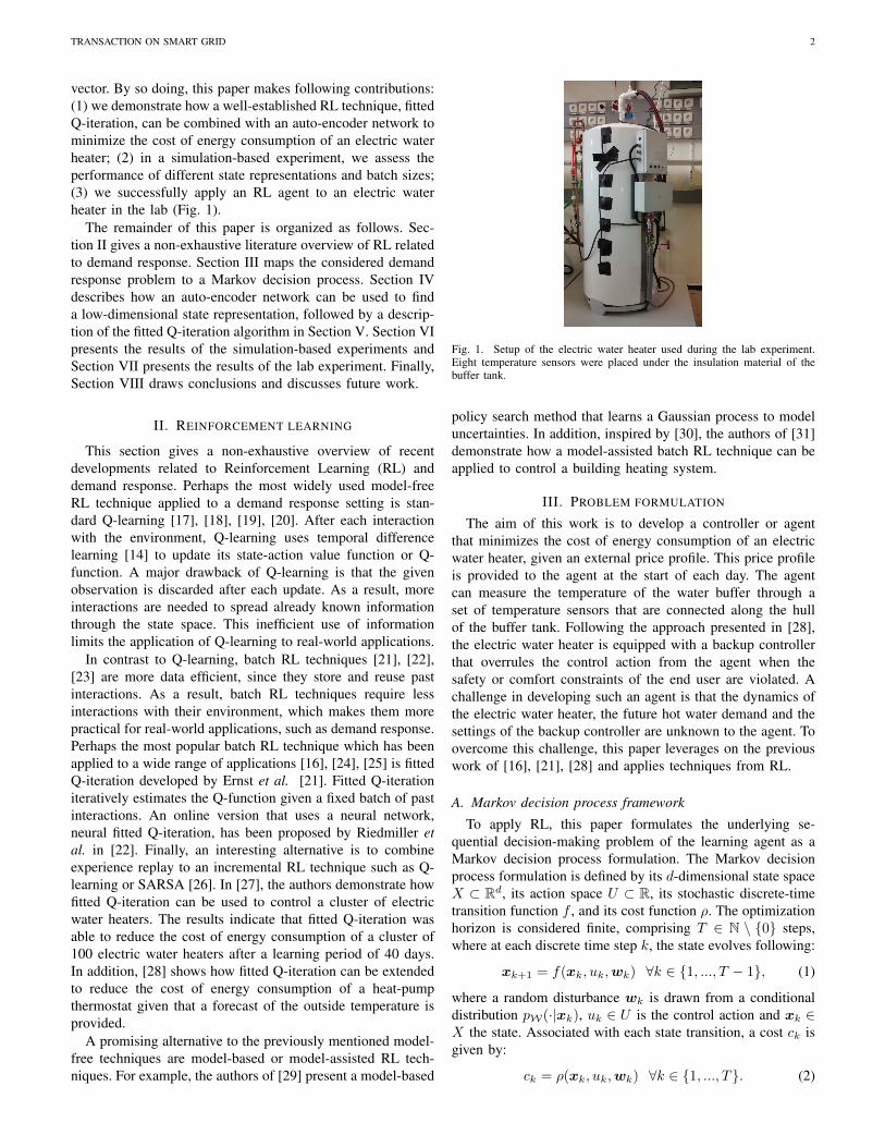
Fig. 3. Simulation-based results of fitted Q-iteration using five state represen-tations and different batch sizes. The full state contains 50 temperature mea-surements. A non-linear dimensionality reduction with Auto-Encoder (AE) isused to find a compact representation of the temperature measurements. Eachmarker point represents the average result of 100 simulation runs.

however as τd decreases the policy directs itself to the mostinteresting state-action pairs. In the evaluation experiments,Q∗ in (15) is linearly scaled between [0, 100] and the τ1 is setto 100 at the start of the experiment, which will result in anequal probability for all actions. The Boltzmann temperatureis updated as follows τd = τd−1 − ∆τ , which increases theprobability of selecting higher valued actions.

VI. SIMULATION-BASED RESULTS

This section describes the results of the simulation-basedexperiments, which use a non-linear stratified tank modelwith 50 temperature layers. A detailed description of thestratified tank model can be found in [3]. The specificationsof the electric water heater are chosen in correspondencewith the electric water heater used during the lab experiment(see Section VII). The simulated electric water heater has apower rating of 2.36kW and has a water buffer of 200 liter.The experiments use realistic hot water profiles with a meandaily consumption of 120 liter [37] and use price informationfrom the Belgian day-ahead [38] and balancing market [39].The learning agent can measure the temperature of the 50temperature layers obtained with the simulation model.

The aim of the first simulation-based experiment is to finda compact state representation using an auto-encoder networkand to assess the impact of the state representation on theperformance of fitted Q-iteration. The second simulation-basedexperiment compares the result of fitted Q-iteration with thedefault thermostat controller.

A. Step 1: feature selection

This experiment compares the performance of fitted Q-iteration combined with different feature representations fordifferent fixed batch sizes. An auto-encoder (AE) network

50 100 150 200 250 300 350

50

100

150

200Day−ahead prices

Days

Cost

[€]

Fitted Q−iteration (AE 5)

Thermostat controller

50 100 150 200 250 300 350

50

100

150

200Intraday imbalance prices

Days

Cost

[€]

Fitted Q−iteration (AE 5)

Thermostat controller

a

b

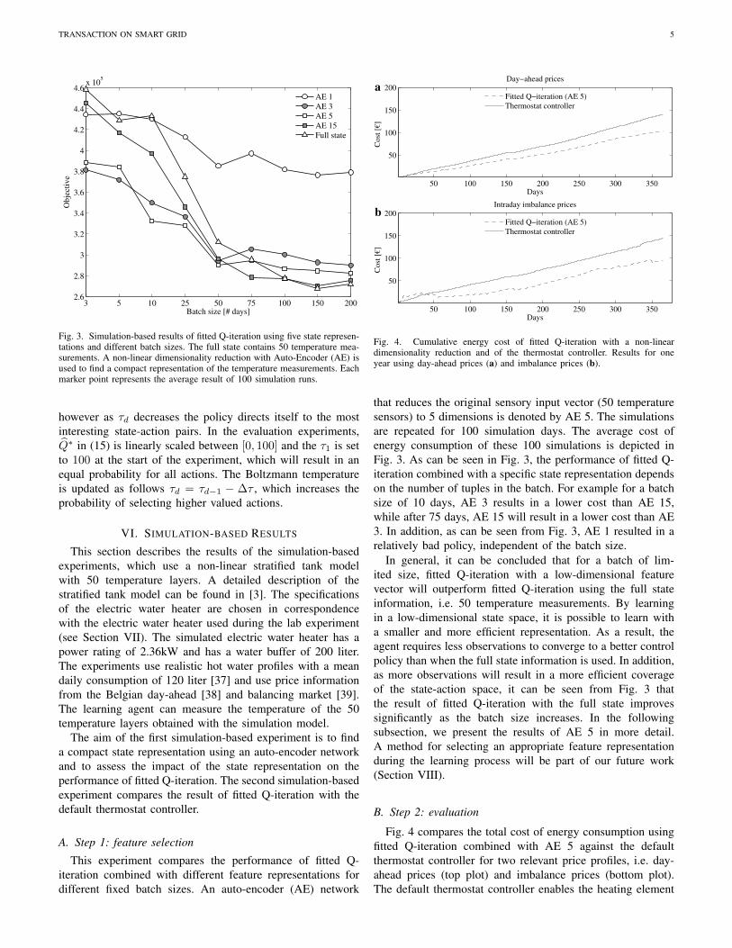
Fig. 4. Cumulative energy cost of fitted Q-iteration with a non-lineardimensionality reduction and of the thermostat controller. Results for oneyear using day-ahead prices (a) and imbalance prices (b).

that reduces the original sensory input vector (50 temperaturesensors) to 5 dimensions is denoted by AE 5. The simulationsare repeated for 100 simulation days. The average cost ofenergy consumption of these 100 simulations is depicted inFig. 3. As can be seen in Fig. 3, the performance of fitted Q-iteration combined with a specific state representation dependson the number of tuples in the batch. For example for a batchsize of 10 days, AE 3 results in a lower cost than AE 15,while after 75 days, AE 15 will result in a lower cost than AE3. In addition, as can be seen from Fig. 3, AE 1 resulted in arelatively bad policy, independent of the batch size.

In general, it can be concluded that for a batch of lim-ited size, fitted Q-iteration with a low-dimensional featurevector will outperform fitted Q-iteration using the full stateinformation, i.e. 50 temperature measurements. By learningin a low-dimensional state space, it is possible to learn witha smaller and more efficient representation. As a result, theagent requires less observations to converge to a better controlpolicy than when the full state information is used. In addition,as more observations will result in a more efficient coverageof the state-action space, it can be seen from Fig. 3 thatthe result of fitted Q-iteration with the full state improvessignificantly as the batch size increases. In the followingsubsection, we present the results of AE 5 in more detail.A method for selecting an appropriate feature representationduring the learning process will be part of our future work(Section VIII).

B. Step 2: evaluation

Fig. 4 compares the total cost of energy consumption usingfitted Q-iteration combined with AE 5 against the defaultthermostat controller for two relevant price profiles, i.e. day-ahead prices (top plot) and imbalance prices (bottom plot).The default thermostat controller enables the heating element

TRANSACTION ON SMART GRID 6

0 48 96 144 192 240 28810

20

30

40

50

60

70

Time [15 min]

Tem

per

ature

[°C

]

T1,…,T

50 (Temperature layers)

0 48 96 144 192 240 2880

1

2

3

Pow

er [

kW

]

Time [15 min]

0 48 96 144 192 240 2880

50

100

150

Pri

ce [

€/M

Wh]

Power Price

a

b

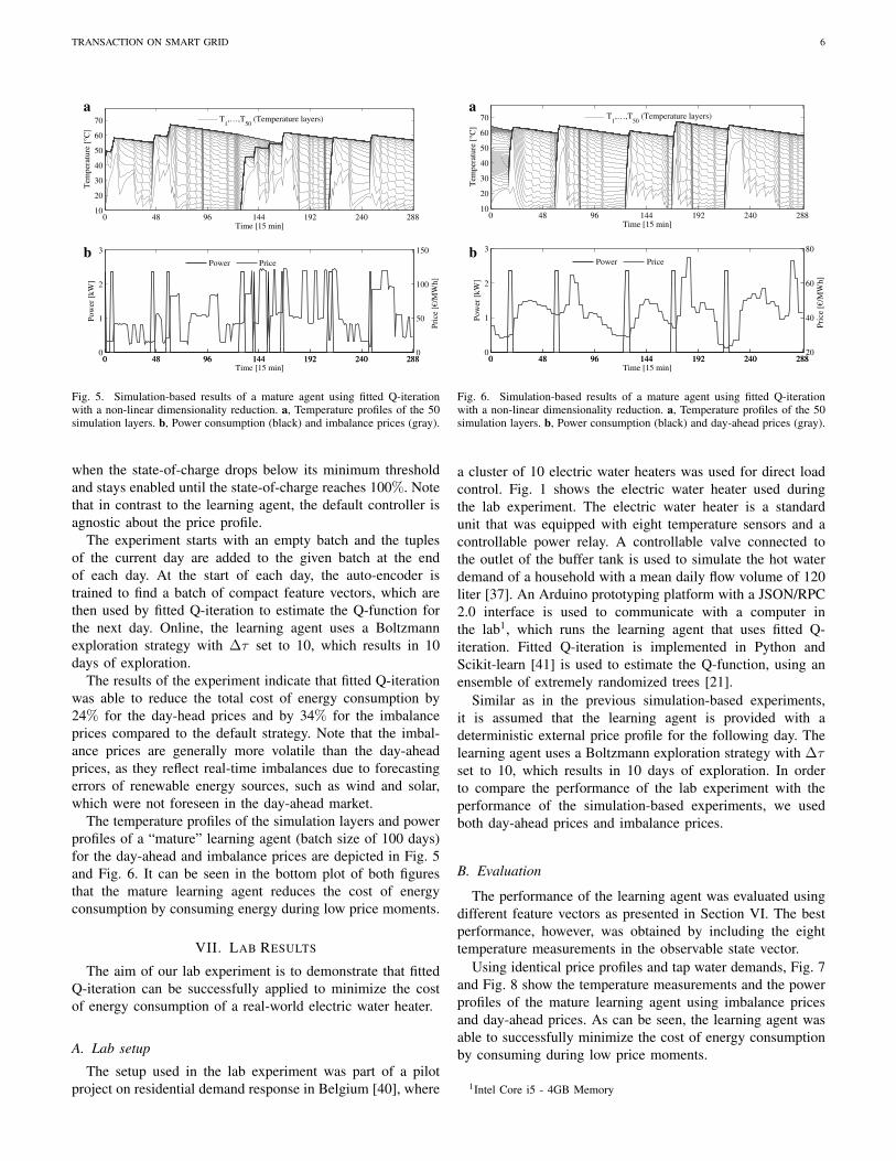
Fig. 5. Simulation-based results of a mature agent using fitted Q-iterationwith a non-linear dimensionality reduction. a, Temperature profiles of the 50simulation layers. b, Power consumption (black) and imbalance prices (gray).

when the state-of-charge drops below its minimum thresholdand stays enabled until the state-of-charge reaches 100%. Notethat in contrast to the learning agent, the default controller isagnostic about the price profile.

The experiment starts with an empty batch and the tuplesof the current day are added to the given batch at the endof each day. At the start of each day, the auto-encoder istrained to find a batch of compact feature vectors, which arethen used by fitted Q-iteration to estimate the Q-function forthe next day. Online, the learning agent uses a Boltzmannexploration strategy with ∆τ set to 10, which results in 10days of exploration.

The results of the experiment indicate that fitted Q-iterationwas able to reduce the total cost of energy consumption by24% for the day-head prices and by 34% for the imbalanceprices compared to the default strategy. Note that the imbal-ance prices are generally more volatile than the day-aheadprices, as they reflect real-time imbalances due to forecastingerrors of renewable energy sources, such as wind and solar,which were not foreseen in the day-ahead market.

The temperature profiles of the simulation layers and powerprofiles of a “mature” learning agent (batch size of 100 days)for the day-ahead and imbalance prices are depicted in Fig. 5and Fig. 6. It can be seen in the bottom plot of both figuresthat the mature learning agent reduces the cost of energyconsumption by consuming energy during low price moments.

VII. LAB RESULTS

The aim of our lab experiment is to demonstrate that fittedQ-iteration can be successfully applied to minimize the costof energy consumption of a real-world electric water heater.

A. Lab setup

The setup used in the lab experiment was part of a pilotproject on residential demand response in Belgium [40], where

0 48 96 144 192 240 28810

20

30

40

50

60

70

Time [15 min]

Tem

per

atu

re [

°C]

T1,…,T

50 (Temperature layers)

0 48 96 144 192 240 2880

1

2

3

Po

wer

[k

W]

Time [15 min]

0 48 96 144 192 240 28820

40

60

80

Pri

ce [

€/M

Wh

]

Power Price

a

b

Fig. 6. Simulation-based results of a mature agent using fitted Q-iterationwith a non-linear dimensionality reduction. a, Temperature profiles of the 50simulation layers. b, Power consumption (black) and day-ahead prices (gray).

a cluster of 10 electric water heaters was used for direct loadcontrol. Fig. 1 shows the electric water heater used duringthe lab experiment. The electric water heater is a standardunit that was equipped with eight temperature sensors and acontrollable power relay. A controllable valve connected tothe outlet of the buffer tank is used to simulate the hot waterdemand of a household with a mean daily flow volume of 120liter [37]. An Arduino prototyping platform with a JSON/RPC2.0 interface is used to communicate with a computer inthe lab1, which runs the learning agent that uses fitted Q-iteration. Fitted Q-iteration is implemented in Python andScikit-learn [41] is used to estimate the Q-function, using anensemble of extremely randomized trees [21].

Similar as in the previous simulation-based experiments,it is assumed that the learning agent is provided with adeterministic external price profile for the following day. Thelearning agent uses a Boltzmann exploration strategy with ∆τset to 10, which results in 10 days of exploration. In orderto compare the performance of the lab experiment with theperformance of the simulation-based experiments, we usedboth day-ahead prices and imbalance prices.

B. Evaluation

The performance of the learning agent was evaluated usingdifferent feature vectors as presented in Section VI. The bestperformance, however, was obtained by including the eighttemperature measurements in the observable state vector.

Using identical price profiles and tap water demands, Fig. 7and Fig. 8 show the temperature measurements and the powerprofiles of the mature learning agent using imbalance pricesand day-ahead prices. As can be seen, the learning agent wasable to successfully minimize the cost of energy consumptionby consuming during low price moments.

1Intel Core i5 - 4GB Memory

TRANSACTION ON SMART GRID 7

0 48 96 144 192 240 28820

30

40

50

60

70

Time [15 min]

Tem

per

ature

[°C

]

T1,…,T

8 (Temperature sensors)

0 48 96 144 192 240 2880

1

2

3

Pow

er [

kW

]

Time [15 min]

0 48 96 144 192 240 2880

50

100

150

Pri

ce [

€/M

Wh]

Power Price

a

b

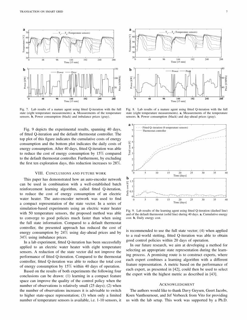
Fig. 7. Lab results of a mature agent using fitted Q-iteration with the fullstate (eight temperature measurements). a, Measurements of the temperaturesensors. b, Power consumption (black) and imbalance prices (gray).

Fig. 9 depicts the experimental results, spanning 40 days,of fitted Q-iteration and the default thermostat controller. Thetop plot of this figure indicates the cumulative costs of energyconsumption and the bottom plot indicates the daily costs ofenergy consumption. After 40 days, fitted Q-iteration was ableto reduce the cost of energy consumption by 15% comparedto the default thermostat controller. Furthermore, by excludingthe first ten exploration days, this reduction increases to 28%.

VIII. CONCLUSIONS AND FUTURE WORK

This paper has demonstrated how an auto-encoder networkcan be used in combination with a well-established batchreinforcement learning algorithm, called fitted Q-iteration,to reduce the cost of energy consumption of an electricwater heater. The auto-encoder network was used to finda compact representation of the state vector. In a series ofsimulation-based experiments using an electric water heaterwith 50 temperature sensors, the proposed method was ableto converge to good policies much faster than when usingthe full state information. Compared to a default thermostatcontroller, the presented approach has reduced the cost ofenergy consumption by 24% using day-ahead prices and by34% using imbalance prices.

In a lab experiment, fitted Q-iteration has been successfullyapplied to an electric water heater with eight temperaturesensors. A reduction of the state vector did not improve theperformance of fitted Q-iteration. Compared to the thermostatcontroller, fitted Q-iteration was able to reduce the total costof energy consumption by 15% within 40 days of operation.

Based on the results of both experiments the following fourconclusions can be drawn: (1) learning in a compact featurespace can improve the quality of the control policy when thenumber of observations is relatively small (25 days); (2) whenthe number of observations increases it is advisable to switchto higher state-space representation; (3) when only a limitednumber of temperature sensors is available, i.e. 1-10 sensors, it

0 48 96 144 192 240 28820

30

40

50

60

70

Time [15 min]

Tem

per

ature

[°C

]

T1,…,T

8 (Temperature sensors)

0 48 96 144 192 240 2880

1

2

3

Pow

er [

kW

]

Time [15 min]

0 48 96 144 192 240 28820

40

60

80

Pri

ce [

€/M

Wh]

Power Price

a

b

Fig. 8. Lab results of a mature agent using fitted Q-iteration with the fullstate (eight temperature measurements). a, Measurements of the temperaturesensors. b, Power consumption (black) and day-ahead prices (gray).

0 5 10 15 20 25 30 35 400

1

2

3

4

5

6

7

8

Time [days]

Tota

l co

st [

€]

Fitted Q−iteration (8 temperature sensors)

Thermostat controller

0 5 10 15 20 25 30 35 40

0

0.5

1

1.5

Time [days]

Dai

ly c

ost

[€]

a

b

Fig. 9. Lab results of the learning agent using fitted Q-iteration (dashed line)and of the default thermostat (solid line) during 40 days. a, Cumulative energycost. b, Daily energy cost.

is recommended to use the full state vector; (4) when appliedto a real-world stetting, fitted Q-iteration was able to obtaingood control policies within 20 days of operation.

In our future research, we aim at developing a method forselecting an appropriate state representation during the learn-ing process. A promising route is to construct experts, whereeach expert combines a learning algorithm with a differentfeature representation. A metric based on the performance ofeach expert, as presented in [42], could then be used to selectthe expert with the highest metric as described in [43].

ACKNOWLEDGMENT

The authors would like to thank Davy Geysen, Geert Jacobs,Koen Vanthournout, and Jef Verbeeck from Vito for providingus with the lab setup. This work was supported by a Ph.D.

TRANSACTION ON SMART GRID 8

grant of the Institute for the Promotion of Innovation throughScience and Technology in Flanders (IWT-Vlaanderen) and byStable MultI-agent LEarnIng for neTworks (SMILE-IT).

REFERENCES

[1] F. Birol et al., “World Energy Outlook 2013: Renewable En-ergy Outlook, An annual report released by the International En-ergy Agency,” http://www.worldenergyoutlook.org/media/weowebsite/2013, Paris, France, [Online: accessed July 21, 2015].

[2] B. Hastings, “Ten years of operating experience with a remote controlledwater heater load management system at detroit edison,” IEEE Trans.on Power Apparatus and Syst., no. 4, pp. 1437–1441, 1980.

[3] K. Vanthournout, R. D’hulst, D. Geysen, and G. Jacobs, “A smartdomestic hot water buffer,” IEEE Trans. on Smart Grid, vol. 3, no. 4,pp. 2121–2127, Dec. 2012.

[4] U.S. Department of Energy, “Energy cost calculator forelectric and gas water heaters,” http://energy.gov/eere/femp/energy-cost-calculator-electric-and-gas-water-heaters-0#output,[Online: accessed November 10, 2015].

[5] R. Diao, S. Lu, M. Elizondo, E. Mayhorn, Y. Zhang, and N. Samaan,“Electric water heater modeling and control strategies for demandresponse,” in Proc. 2012 IEEE Power and Energy Society GeneralMeeting,, pp. 1–8.

[6] S. Iacovella, K. Lemkens, F. Geth, P. Vingerhoets, G. Deconinck,R. D’Hulst, and K. Vanthournout, “Distributed voltage control mech-anism in low-voltage distribution grid field test,” in Proc. 4th IEEE PESInnov. Smart Grid Technol. Conf. (ISGT Europe), Oct 2013, pp. 1–5.

[7] S. Koch, J. L. Mathieu, and D. S. Callaway, “Modeling and control ofaggregated heterogeneous thermostatically controlled loads for ancillaryservices,” in Proc. 17th IEEE Power Sys. Comput. Conf. (PSCC),Stockholm, Sweden, Aug. 2011, pp. 1–7.

[8] J. Mathieu and D. Callaway, “State estimation and control of hetero-geneous thermostatically controlled loads for load following,” in Proc.45th Hawaii Int. Conf. on System Science (HICSS), Maui, HI, Jan. 2012,pp. 2002–2011.

[9] F. Sossan, A. M. Kosek, S. Martinenas, M. Marinelli, and H. Bindner,“Scheduling of domestic water heater power demand for maximizing PVself-consumption using model predictive control,” in Proc. 4th IEEE PESInnov. Smart Grid Technol. Conf. (ISGT Europe), Oct 2013, pp. 1–5.

[10] E. F. Camacho and C. Bordons, Model Predictive Control, 2nd ed.London, UK: Springer London, 2004.

[11] J. Cigler, D. Gyalistras, J. Siroky, V. Tiet, and L. Ferkl, “Beyond theory:the challenge of implementing model predictive control in buildings,” inProc. 11th REHVA World Congress (CLIMA), Czech Republic, Prague,2013.

[12] Y. Ma, “Model predictive control for energy efficient buildings,” Ph.D.dissertation, University of California Berkeley, Mechanical Engineering,Berkeley, CA, 2012.

[13] M. Maasoumy, M. Razmara, M. Shahbakhti, and A. Sangiovanni Vincen-telli, “Selecting building predictive control based on model uncertainty,”in Proc. American Control Conference (ACC), Portland, OR, June 2014,pp. 404–411.

[14] R. S. Sutton and A. G. Barto, Reinforcement Learning: An Introduction.Cambridge, MA: MIT Press, 1998.

[15] D. Ernst, M. Glavic, F. Capitanescu, and L. Wehenkel, “Reinforcementlearning versus model predictive control: a comparison on a powersystem problem,” IEEE Trans. Syst., Man, Cybern., Syst., vol. 39, no. 2,pp. 517–529, 2009.

[16] S. Lange and M. Riedmiller, “Deep auto-encoder neural networks inreinforcement learning,” in Proc. IEEE 2010 Int. Joint Conf. on NeuralNetworks (IJCNN), Barcelona, Spain, July 2010, pp. 1–8.

[17] E. C. Kara, M. Berges, B. Krogh, and S. Kar, “Using smart devices forsystem-level management and control in the smart grid: A reinforcementlearning framework,” in Proc. 3rd IEEE Int. Conf. on Smart GridCommun. (SmartGridComm), Tainan, Taiwan, Nov. 2012, pp. 85–90.

[18] G. P. Henze and J. Schoenmann, “Evaluation of reinforcement learningcontrol for thermal energy storage systems,” HVAC&R Research, vol. 9,no. 3, pp. 259–275, 2003.

[19] Z. Wen, D. O’Neill, and H. Maei, “Optimal demand response usingdevice-based reinforcement learning,” IEEE Trans. on Smart Grid,vol. 6, no. 5, pp. 2312–2324, Sept 2015.

[20] M. Gonzalez, R. Luis Briones, and G. Andersson, “Optimal bidding ofplug-in electric vehicles in a market-based control setup,” in Proc. 18thIEEE Power Sys. Comput. Conf. (PSCC), Wroclaw, Poland, 2014, pp.1–7.

[21] D. Ernst, P. Geurts, and L. Wehenkel, “Tree-based batch mode reinforce-ment learning,” Journal of Machine Learning Research, pp. 503–556,2005.

[22] M. Riedmiller, “Neural fitted Q-iteration–first experiences with a dataefficient neural reinforcement learning method,” in Proc. 16th EuropeanConference on Machine Learning (ECML), vol. 3720. Porto, Portugal:Springer, Oct. 2005, p. 317.

[23] V. Mnih, K. Kavukcuoglu, D. Silver, A. A. Rusu, J. Veness, M. G.Bellemare, A. Graves, M. Riedmiller, A. K. Fidjeland, G. Ostrovskiet al., “Human-level control through deep reinforcement learning,”Nature, vol. 518, no. 7540, pp. 529–533, 2015.

[24] M. Riedmiller, T. Gabel, R. Hafner, and S. Lange, “Reinforcementlearning for robot soccer,” Autonomous Robots, vol. 27, no. 1, pp. 55–73,2009.

[25] R. Fonteneau, L. Wehenkel, and D. Ernst, “Variable selection fordynamic treatment regimes: a reinforcement learning approach,” in Proc.European Workshop on Reinforcement Learning (EWRL), Villeneuved’Ascq, France, 2008.

[26] S. Adam, L. Busoniu, and R. Babuska, “Experience replay for real-time reinforcement learning control,” IEEE Trans. on Syst., Man, andCybern., Part C: Applications and Reviews, vol. 42, no. 2, pp. 201–212,2012.

[27] F. Ruelens, B. Claessens, S. Vandael, S. Iacovella, P. Vingerhoets, andR. Belmans, “Demand response of a heterogeneous cluster of electricwater heaters using batch reinforcement learning,” in Proc. 18th IEEEPower Sys. Comput. Conf. (PSCC), Wrocław, Poland, Aug. 2014, pp.1–8.

[28] F. Ruelens, B. Claessens, S. Vandael, B. De Schutter, R. Babuska, andR. Belmans, “Residential Demand Response Applications Using BatchReinforcement Learning,” Submitted to IEEE Trans. on Smart Grid(http://arxiv.org/pdf/1504.02125.pdf), Apr. 2015.

[29] M. Deisenroth and C. E. Rasmussen, “PILCO: A model-based anddata-efficient approach to policy search,” in Proceedings of the 28thInternational Conference on machine learning (ICML-11), 2011, pp.465–472.

[30] T. Lampe and M. Riedmiller, “Approximate model-assisted neural fittedq-iteration,” in 2014 International Joint Conference on Neural Networks(IJCNN), July 2014, pp. 2698–2704.

[31] G. T. Costanzo, S. Iacovella, F. Ruelens, T. Leurs, and B. Claessens,“Experimental analysis of data-driven control for a building heatingsystem,” CoRR, vol. abs/1507.03638, 2015. [Online]. Available:http://arxiv.org/abs/1507.03638

[32] R. Bellman, Dynamic Programming. New York, NY: Dover Publica-tions, 1957.

[33] W. Curran, T. Brys, M. Taylor, and W. Smart, “Using PCA to efficientlyrepresent state spaces,” in The 12th European Workshop on Reinforce-ment Learning (EWRL 2015), Lille, France, 2015.

[34] D. Bertsekas and J. Tsitsiklis, Neuro-Dynamic Programming. Nashua,NH: Athena Scientific, 1996.

[35] M. Scholz and R. Vigario, “Nonlinear PCA: a new hierarchical ap-proach.” in ESANN, 2002, pp. 439–444.

[36] L. P. Kaelbling, M. L. Littman, and A. W. Moore, “Reinforcementlearning: A survey,” Journal of Artificial Intelligence Research, pp. 237–285, 1996.

[37] U. Jordan and K. Vajen, “Realistic domestic hot-water profiles indifferent time scales: Report for the international energy agency, solarheating and cooling task (IEA-SHC),” Universitat Marburg, Marburg,Germany, Tech. Rep., 2001.

[38] “Belpex - Belgian power exchange,” http://www.belpex.be/, [Online:accessed March 21, 2015].

[39] “Elia - Belgian power exchange,” http://www.belpex.be/, [Online: ac-cessed March 21, 2015].

[40] B. Dupont, P. Vingerhoets, P. Tant, K. Vanthournout, W. Cardinaels,T. De Rybel, E. Peeters, and R. Belmans, “LINEAR breakthroughproject: Large-scale implementation of smart grid technologies in distri-bution grids,” in Proc. 3rd IEEE PES Innov. Smart Grid Technol. Conf.(ISGT Europe), Berlin, Germany, Oct. 2012, pp. 1–8.

[41] F. Pedregosa, G. Varoquaux, A. Gramfort, V. Michel, B. Thirion,O. Grisel, M. Blondel, P. Prettenhofer, R. Weiss, V. Dubourg et al.,“Scikit-learn: Machine learning in Python,” The Journal of MachineLearning Research, vol. 12, pp. 2825–2830, 2011.

[42] R. Fonteneau, S. A. Murphy, L. Wehenkel, and D. Ernst, “Batch modereinforcement learning based on the synthesis of artificial trajectories,”Annals of Operations Research, vol. 208, no. 1, pp. 383–416, 2013.

[43] M. Devaine, P. Gaillard, Y. Goude, and G. Stoltz, “Forecasting electricityconsumption by aggregating specialized experts,” Machine Learning,vol. 90, no. 2, pp. 231–260, 2013.