Trajectory Representation by Nonlinear Scaling of Dynamic MovementPrimitives

Ales Ude1,2, Rok Vuga1, Bojan Nemec1, and Jun Morimoto2†

Abstract— An effective robot trajectory representation shouldencode all relevant aspects of the desired motion. For kinematicrepresentations, this means that both the spatial course of thetrajectory and its speed profile must be specified. The concept ofdynamic movement primitives (DMP) provides a kinematic rep-resentation that fully specifies these two aspects of motion. Theyare, however, not separated from each other within the DMPrepresentation. This can be problematic when movements withsignificant speed variations are compared within movementrecognition and skill learning algorithms. In such comparisonsit is often important to distinguish between the spatial andtemporal aspects of motion. In this paper we propose anew representation based on dynamic movement primitives,where spatial and temporal aspects are well separated. Wedemonstrate the effectiveness of the proposed representation forstatistical learning of robot skills and movement recognition andcompare the performance with standard DMPs, where temporaland spatial aspects of motion are intertwined.

I. INTRODUCTION

Nonlinear dynamic systems, i. e. nonlinear systems of dif-ferential equations, can be effective at representing kinematiccontrol policies that create kinematic target values for robotcontrol [1]. Among various approaches based on dynamicsystems, dynamic movement primitives (DMPs) of Ijspeertet al. [2] have proven to be a popular choice due to theirflexibility. They can be used to represent robot movementswith complex trajectories, they include free parameters forlearning and optimization, they are not explicitly dependenton time, are robust to perturbations, allow easy modulationto adjust to joint limits or speed up or slow down themovement, etc. For these reasons DMPs are widely used inrobotics, including for movement imitation [3], policy search[4], [5], statistical learning from multiple demonstrations [6],[7], sharing of knowledge for efficient generalization [8],adaptation of trajectories to new endpoints [9], adaptation tothe recorded sensory data [10], [11], and coupling of dual-arm movements [12], [13].

The focus of our recent work was on an extension ofdynamic movement primitives for learning of speed profiles[14], [15]. Additional parameters were introduced in the

†The research leading to these results has received funding from the Euro-pean Community’s Seventh Framework Programme under grant agreementno. 270273, Xperience, and from the Slovenian Research Agency undergrant agreement no. J2-7360. It was further supported by MIC-SCOPE,by the New Energy and Industrial Technology Development Organization(NEDO), by JSPS KAKENHI JP16H06565, and by the Strategic ResearchProgram for Brain Science from AMED.

1Humanoid and Cognitive Robotics Lab, Dept. of Automatics, Biocyber-netics, and Robotics, Jozef Stefan Institute, Ljubljana, Slovenia.

2Dept. of Brain Robot Interface, ATR Computational NeuroscienceLaboratories, Kyoto, Japan.

proposed representation that allow for nonuniform temporalscaling of the desired trajectories. With this representation,we were able to speed up or slow down trajectories withoutaffecting the spatial course of movement. In this paper weshow that the representation proposed in [14], [15] is relatedto the parametrization of dynamic systems by arc lengthinstead of time and develop a new representation, which wecall arc length dynamic movement primitives (AL-DMPs).Spatial and temporal aspects of motion are well separatedin AL-DMPs. We demonstrate that the newly developedrepresentation significantly improves the power of DMPswhen applied to the problem of statistical learning of robotmovements and movement recognition.

Other recent research that addresses the problem of timealignment within the framework of DMPs includes the workof Englert et al. on probabilistic movement primitives [16]and Ben Amor et al. on interaction primitives [17], wheremultiple trajectories are time aligned using dynamic timewarping [18]. On the other hand, Ewerton et al. [19] applieda probabilistic approach to solve the alignment problem.The advantage of our approach is the parametrization ofmovement through a natural parameter, i. e. the arc length,which provides alignment without the need for an algorith-mic comparison between different trajectories.

In the rest of the paper we first introduce the concept of arclength dynamic movement primitives. Next we discuss theestimation of AL-DMPs and robot control with AL-DMPs.In Section V-B we analyze the application of AL-DMPsto the problems of statistical learning of motor skills andmovement recognition. The significant advantages of AL-DMPs compared to standard DMPs have been demonstrated.

II. TRAJECTORY PARAMETERIZATION AND ARC LENGTHOF A CURVE

A DMP for a single degree of freedom point-to-pointmovement y is defined by the following set of nonlineardifferential equations [2]

τ z = αz(βz(g − y)− z) + F (x), (1)τ y = z, (2)

where x is the phase variable, z is the scaled velocity of themovement, g is the desired final position on the movement,and F is a nonlinear forcing term. With the choice τ > 0and αz = 4βz , the linear part of equation system (1)– (2) becomes critically damped and y, z monotonicallyconverge to a unique attractor point at y = g, z = 0 [2].F (x) is defined as a linear combination of N nonlinearradial basis functions, which enables the robot to follow any

2016 IEEE/RSJ International Conference on Intelligent Robots and Systems (IROS)Daejeon Convention CenterOctober 9-14, 2016, Daejeon, Korea

978-1-5090-3761-2/16/$31.00 ©2016 IEEE 4728

0 0.2 0.4 0.6 0.8 1time [sec]

-3

-2

-1

0

1

2jo

int a

ngle

[rad

]

faster trajectory j1faster trajectory j2slower trajectory j1slower trajectory j2

-3 -2.5 -2 -1.5 -1joint angle 1 [rad]

0

0.5

1

1.5

2

join

t ang

le 2

[rad

]

faster trajectoryslower trajectory

0 0.2 0.4 0.6 0.8 1normalized arc length [unitless]

0

5

10

15

20

25

30

spee

d [ra

d/se

c]

faster trajectoryslower trajectory

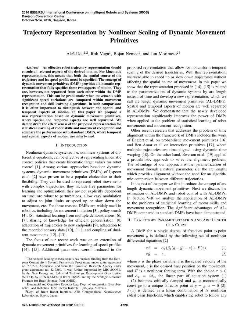
Fig. 1: Simulation results for movement estimation with AL-DMPs. The left graph shows trajectories of a simulatedtwo degrees of freedom robot executed at two different speeds, resulting in spatially equivalent but temporally differentmovements. The faster movement was obtained by multiplying the speed of the slower movement by a factor of2(t + 1)e(t+1)2−2, t ∈ [0, T ], T = 0.5345, where T is the interval of the faster movement. This is a nonlinear speedscaling that completely changes the spatial parameters w defining the forcing term of the standard DMP. The middle graphshows the reproduction of the spatial course of movement by AL-DMP. Parameters w of AL-DMPs and consequently thespatial courses of the two movements are identical up to the errors caused by numerical differentiation. The right graphshows the estimated speed s of both movements as a function of normalized arc length, i. e. s/L. It is clear that the change isnonlinear, hence it cannot be reproduced by simply changing the parameter τ in the standard DMP. These graphs demonstratethat the proposed representation effectively separates the spatial and temporal aspects of movements.

smooth trajectory from the initial position y0 to the finalconfiguration g

F (x) =

∑Ni=1 wiΨi(x)∑Ni=1 Ψi(x)

x(g − y0), (3)

Ψi(x) = exp(−hi (x− ci)2

). (4)

ci are the centers of Gaussians distributed along the phaseof the movement and hi their widths. The phase x has beenintroduced to avoid explicit time dependency. Its evolutionfollows the first order linear dynamics

τ x = −αxx, (5)

where αx > 0 and x(0) = 1. For each degree of freedom, theweights wi should be adjusted so that the desired behavioris achieved. To control a robot with more than one degreeof freedom, the trajectory of every degree of freedom isrepresented with its own equation system (1) – (2), but withthe common phase (5) to synchronize them.

The above formulation has been shown to have manyadvantageous properties for robot control [1], [6], [2]. Withthis representation, however, it is often difficult to comparedifferent movement promitives between each other becauseEqs. (1) – (2) contain time derivatives. Time derivativesare dependent both on speed and shape of movement anddo not distinguish between the two. As it is well knownfrom basic calculus, speed and form can be separated byparameterization with the arc length. The arc length of atime-parameterized trajectory y(t) is given by

s(t) =

∫ t

0

‖y(u)‖du. (6)

The speed of movement can be calculated as the timederivative of s, which is given by

s(t) = ‖y(t)‖. (7)

We will also need the length of the trajectory, which wedenote here by L and can be calculated as follows

L =

∫ T

0

‖y(t)‖dt, (8)

where T is the duration of the movement.Let’s assume now that a trajectory is parameterized by the

arc length instead of time. Just like the time-parameterizedmovements, we can approximate arc length-parameterizedmovements with a second order dynamic system

Lz′ = αz(βz(g − y)− z) + F (x), (9)Ly′ = z, (10)

where all derivatives are now taken not with respect to timebut with respect to the arc length (this derivative is denotedby ′). Similarly, the phase equation (5) becomes

Lx′ = −αxx. (11)

The time constant τ, which is used in standard DMPs tospeed-up or slow-down the movement during its executionby the robot, was replaced by arc length L > 0, whichis defined by Eq. (8). We name this new formulation arclength dynamic movement primitive, or AL-DMP. Figure 1shows that an AL-DMP effectively separates the spatial andtemporal component of motion. Just like the time-dependentequation (5), the arc length dependent phase equation has ananalytical solution. It is given by

x(s) = exp(−αx

s

L

). (12)

Note that due to the replacement of τ with arc length L,the phase is always defined on the same interval regardlessof the length of the trajectory. Consequently, 1 ≥ x ≥exp(−αx), ∀s ∈ [0, L].

4729

III. ESTIMATION OF AL-DMPS

To estimate the parameters of DMPs, we are usually giventraining data in a form of a sequence of trajectory points

G = {yk, tk}Kk=1,yk ∈ Rd, (13)

where d is the number of the robot’s degrees of freedom,t1 = 0, tK = T . The time derivatives yk, yk are also neededto compute a standard DMP, but they are usually estimatednumerically. To approximate these data with the equationsystem (9) – (11), we first sample the trajectory with respectto s. This can be achieved by calculating the arc length steps

sk =

∫ tk

0

‖y(t)‖dt ∼ Trapzd(k), (14)

where the trapezoidal rule was used for numerical quadrature

Trapzd(k) ={∆t(

12‖y1‖+

∑k−1n=2 ‖yn‖+ 1

2‖yk‖), k ≥ 2

0, k = 1

(15)

to approximate the above integrals. Here we assumed thatthe time step is constant, i. e. ∆t = tk+1 − tk, ∀k, but thisassumption can be relaxed by applying a different numericalquadrature formula. Similarly, the length of the movementcan be estimated by

L =

∫ T

0

‖y(t)‖dt ∼ Trapzd(K), (16)

The time derivatives ‖yn‖ can be computed using standardnumerical differentiation formulas, e. g.

‖yn‖ =‖yn+1 − yn‖

∆t. (17)

From sk, k = 1, . . . ,K, and the input data G, we cancalculate y′k and y′′k by numerical differentiation, e. g.

y′k =yk+ik − yk

sk+ik − sk, y′′k =

y′k+ik− y′k

sk+ik − sk. (18)

In practice we need to make sure that the arc length step∆s is large enough for numerically stable calculation ofderivatives (18) because unlike the time step, the arc lengthstep is not uniform in the sampled trajectory. This can bedone by choosing ik to be the smallest index |ik| (positive ornegative) so that |sk+ik −sk| ≥ δ, where δ > 0 is a constantspecifying the minimum step. Otherwise the calculation ofnumerical derivatives can become unstable at locations withzero speed, i. e. where s = 0.

We are now ready to estimate the free parameters of AL-DMPs, i. e. weights wi of radial basis functions as specifiedin Eq. (3). As with standard DMPs, we first rewrite theequation system (9) – (10) as a single second-order system

F (x) = L2y′′ − αz(βz(g − y)− Ly′). (19)

From these formulas we can calculate wi by solving thefollowing system of linear equations

Aw = f , (20)

with

w =

w1

...wN

, f =

f1...fK

, (21)

the (K ×N) system matrix A defined as

A = (g − y0)

ψ1(x1)x1∑Nj=1 ψj(x1)

· · · ψN (x1)x1∑Nj=1 ψj(x1)

......

...ψ1(xK)xK∑Nj=1 ψj(xK)

· · · ψN (xK)xK∑Nj=1 ψj(xK)

,and

fk = L2y′′k − αz(βz(g − yk)− Ly′k), (22)

xk = exp(−αx

skL

). (23)

Here we assumed that F is defined as in (3). For a givennumber N of radial basis functions Ψi, which are definedas in (4), we calculate their parameters as follows: ci =

exp(−αx

i−1N−1

), hi =

2

(ci+1 − ci)2, i = 1, . . . , N − 1,

hN = hN−1. A set of weights that solves linear equationsystem (20) in a least squares sense is then calculated using

w = A+f , (24)

where A+ denotes the Moore-Penrose pseudo-inverse of thesystem matrix A.

Eqs. (9) – (11) do not contain all information needed tocontrol the robot. What’s missing is the speed of motion. Ateach phase x on the trajectory {y,y′,y′′}, we need to knowalso the speed, or equivalently, the time derivative of the arclength, i. e. s. We use radial basis functions to approximates at phase x

s(x) = 1 +

∑Ni=1 v

si Ψi(x)∑N

i=1 Ψi(x)x. (25)

The time derivative of s can be calculated using formula (7).Thus we obtain the following system of linear equations

‖yk‖ − 1 =

∑Ni=1 v

si Ψi(xk)∑N

i=1 Ψi(xk)xk, k = 1. . . . ,K. (26)

(26) is a standard overdetermined linear equation system invsi that can be solved in a similar way as equation system(20). Note that beyond the demonstrated trajectory, s asdefined by Eq. (25) converges to 1 as the phase x tends tozero. This property is important to ensure the convergence ofan AL-DMP to its desired final configuration g. To enabletorque control, the derivative of speed is also needed. Wewrite

s(x) =

∑Ni=1 v

ai Ψi(x)∑N

i=1 Ψi(x)x. (27)

The data for estimating the parameters vai are obtained bynumerical differentiation of s as estimated by Eq. (14).Unlike s defined by (25), which converges to 1, s defined by(27) converges to zero beyond the end of the demonstratedtrajectory.

4730

Fig. 2: Teaching of joint space trajectories from the unique starting point (left) to via point (middle) and back (right). Thetrajectories were sampled at 100 Hz. Note that the robot’s end-effector only approximately reaches the via point and thatthe end point is similar but not exactly the same as the starting point.

IV. AL-DMPS IN TIME DOMAIN

While AL-DMPs have many favourable properties forlearning and recognition, they cannot be used directly forcontrol because a robot is controlled at constant time steps,not constant arc length steps. Equivalent, time-dependentequations can be derived by exploiting the relationshipbetween time and arc length derivatives

y =d

dty(s(t)) = y′s, (28)

y =d2

dt2y(s(t)) = y′′s2 + y′s. (29)

We can now express arc length derivatives in terms of timederivatives

y′ =1

sy, (30)

y′′ =1

s3(ys− ys) . (31)

From (30) – (31) and (9) - (10) we obtain

z = Ly′ =L

sy (32)

z = Lys− yss2

, (33)

z′ = Ly′′ =1

sLys− yss2

=1

sz, (34)

and finally, by respectively inserting (28) and (34) into (9)and (10),

Lz = s (αz(βz(g − y)− z) + F (x)) , (35)Ly = sz. (36)

Similarly, the phase equation (11) can be rewritten in anequivalent, time-dependent form

Lx = −sαxx. (37)

A. Control with AL-DMPs

To control a robot at constant time steps, we can integrateEq. (35) – (37), which are expressed in terms of timederivatives, instead of (9) – (11), which are expressed interms of arc length derivatives. The initial values are set toy = y0, z = Ly0/s0, x = 1. Note that s approximatedby Eq. (25) is given as a function of phase. If the second

derivatives are also needed by the controller, as is the casewith torque-controlled systems, they can be calculated from(33)

y =1

L

s2z + ys

s. (38)

This equation involves s, which we estimate using Eq. (27).

B. Stability of AL-DMPs

The arc length s and its derivative s can be learnt onlyalong the demonstrated trajectory. Beyond the end of thelearned trajectory, i. e. for s > L, we have no informationabout the arc length and the speed of movement. Undernormal circumstances, the end of the executed movementcoincides with the attractor point y = g, z = 0, but in caseof perturbations this might not be the case. However, sinces is strictly positive outside of the interval of learning, xdefined by (37) tends to zero as time increases, consequentlys defined by (25) tends to 1 and the equation system (35) –(36) tends to the second order linear system

Lz = αz(βz(g − y)− z), (39)Ly = z, (40)

which has a unique attractor point at y = g, z = 0. Thus justlike standard DMPs, AL-DMPs are guaranteed to convergeto the desired final configuration. Note that s is equal to thespeed of movement only within the training interval; thusthe fact that s tends to 1 outside of the training interval doesnot mean that the speed of movement tends to 1. The actualspeed of movement is specified by Eq. (39) – (40) and tendsto 0, thus the robot is guaranteed to come to rest at the endof integration process.

V. EXPERIMENTAL RESULTS

A. Statistical skill learning with AL-DMPs

The proposed formulation of AL-DMPs has a potential tosignificantly improve the performance of statistical learningalgorithms because it can ensure the proper alignment of thetraining data. This is essential for many learning algorithmsthat analyze the interdependencies between the availableexample trajectories. For example, in statistical learningalgorithms, e. g. [6], multiple user demonstrations are locallyaveraged to generate new movements. Such an averaging pro-cess requires the alignment of example trajectories, which is

4731

0.450.5

0

0.550.6

0.65

z [m

]

0.7

0.2

0.750.8

0.4

x [m]

0.6

0.8

0.80.7

0.610.5

y [m]

0.40.3

0.20.1

01.2-0.1

0.5

0

0.6

z [m

]

0.2

0.7

0.8

0.4

x [m]

0.6

0.8

0.80.7

0.60.51

y [m]

0.40.3

0.20.1

01.2-0.1

0.4

0

0.5

0.6

0.2

z [m

]

0.7

0.4

x [m]

0.6

0.8

0.80.7

0.60.5

y [m]

10.4

0.30.2

0.101.2

-0.1

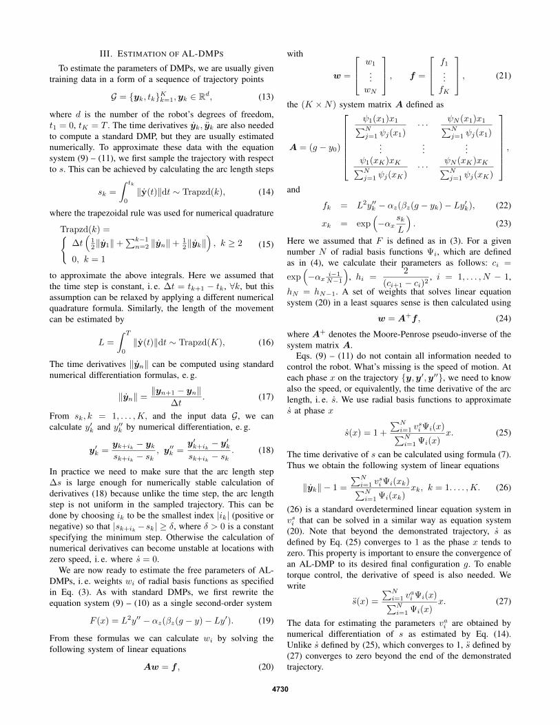
Fig. 3: Three spatial paths generated by statistical trajectory learning using DMP (blue) and AL-DMP representation (red).The training trajectories are shown in black. It is clear that the AL-DMP paths (red) are a better approximation of the data,that they come closer to the via points (shown as stars) and that they exhibit less artifacts not present in the training datathan the DMP paths (blue).

0.10.20.30.40.50.60.70.80.91x

0

0.1

0.2

0.3

0.4

0.5

0.6

0.7

0.8

0.9

1

ds/d

t [1/

s]

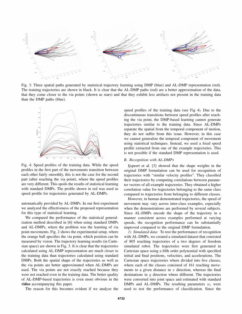
Fig. 4: Speed profiles of the training data. While the speedprofiles in the first part of the movements transition betweeneach other fairly smoothly, this is not the case for the secondpart (after reaching the via point), where the speed profilesare very different. This spoils the results of statistical learningwith standard DMPs. The profile shown in red was used asspeed profile for trajectories generated by AL-DMPs.

automatically provided by AL-DMPs. In our first experimentwe analyzed the effectiveness of the proposed representationfor this type of statistical learning.

We compared the performance of the statistical general-ization method described in [6] when using standard DMPsand AL-DMPs, where the problem was the learning of viapoint movements. Fig. 2 shows the experimental setup, wherethe orange ball specifies the via point, which position can bemeasured by vision. The trajectory learning results (in Carte-sian space) are shown in Fig. 3. It is clear that the trajectoriescalculated using AL-DMP representation are much closer tothe training data than trajectories calculated using standardDMPs. Both the spatial shape of the trajectories as well asthe via points are better approximated when AL-DMPs areused. The via points are not exactly reached because theywere not reached even in the training data. The better qualityof AL-DMP-based trajectories is even more obvious in thevideo accompanying this paper.

The reason for this becomes evident if we analyze the

speed profiles of the training data (see Fig 4). Due to thediscontinuous transitions between speed profiles after reach-ing the via point, the DMP-based learning cannot generatetrajectories similar to the training data. Since AL-DMPsseparate the spatial from the temporal component of motion,they do not suffer from this issue. However, in this casewe cannot generalize the temporal component of movementusing statistical techniques. Instead, we used a fixed speedprofile extracted from one of the example trajectories. Thisis not possible if the standard DMP representation is used.

B. Recognition with AL-DMPs

Ijspeert et al. [3] showed that the shape weights in theoriginal DMP formulation can be used for recognition oftrajectories with “similar velocity profiles”. They classifiedtheir trajectories by computing correlations between parame-ter vectors of all example trajectories. They obtained a highercorrelation value for trajectories belonging to the same classcompared to trajectories from belonging to different classes.

However, in human demonstrated trajectories, the speed ofmovement may vary across inter-class examples, especiallywhen the demonstrations are performed by several subjects.Since AL-DMPs encode the shape of the trajectory in amanner consistent across examples performed at varyingspeeds, the recognition performance can be substantiallyimproved compared to the original DMP formulation.

1) Simulated data: To test the performance of recognitionwith AL-DMPs, we created a simulated dataset that consistedof 805 reaching trajectories of a two degrees of freedomsimulated robot. The trajectories were first generated inCartesian space using a fifth order polynomial with specifiedinitial and final positions, velocities, and accelerations. TheCartesian space trajectories where divided into five classes,where each of the classes consisted of 161 reaching move-ments to a given distance in x direction, whereas the finaldestinations in y direction where different. The trajectorieswere converted into joint space and estimated with standardDMPs and AL-DMPs. The resulting parameters wi wereused to test the performance of classification. Since the

4732

ground truth

AL-DMP

DMP

AL-DMP - modified

DMP - modified

class 1 class 2 class 3 class 4 class 5

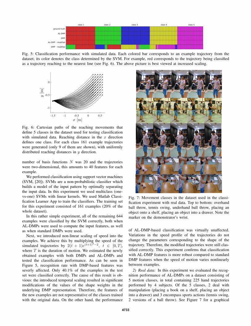
Fig. 5: Classification performance with simulated data. Each colored bar corresponds to an example trajectory from thedataset; its color denotes the class determined by the SVM. For example, red corresponds to the trajectory being classifiedas a trajectory reaching to the nearest line (see Fig. 6). The above picture is best viewed at increased scaling.

x [m]-1.5 -1 -0.5 0 0.5

y[m

]

-1

-0.5

0

Fig. 6: Cartesian paths of the reaching movements thatdefine 5 classes in the dataset used for testing classificationwith simulated data. Reaching distance in the x directiondefines one class. For each class 161 example trajectorieswere generated (only 9 of them are shown), with uniformlydistributed reaching distances in y direction.

number of basis functions N was 20 and the trajectorieswere two-dimensional, this amounts to 40 features for eachexample.

We performed classification using support vector machines(SVM, [20]). SVMs are a non-probabilistic classifier whichbuilds a model of the input pattern by optimally separatingthe input data. In this experiment we used multiclass (one-vs-one) SVMs with linear kernels. We used Matlab Classi-fication Learner App to train the classifiers. The training setfor this experiment consisted of 161 examples (20% of thewhole dataset).

In this rather simple experiment, all of the remaining 644examples were classified by the SVM correctly, both whenAL-DMPs were used to compute the input features, as wellas when standard DMPs were used.

Next, we introduced non-linear scaling of speed into theexamples. We achieve this by multiplying the speed of thesimulated trajectories by 2(t + 1)e(t+1)2−2, t ∈ [0, T ],where T is the duration of motion. We estimated the newlyobtained examples with both DMPs and AL-DMPs andtested the classification performance. As can be seen inFigure 5, recognition rate with DMP-based features wasseverly affected. Only 40.1% of the examples in the testset were classified correctly. The cause of this result is ob-vious: the introduced temporal scaling resulted in significantmodifications of the values of the shape weights in theunderlying DMP representation. Therefore, the features ofthe new examples are not representative of the classes trainedwith the original data. On the other hand, the performance

Fig. 7: Movement classes in the dataset used in the classi-fication experiment with real data. Top to bottom: overhandball throw, tennis swing, underhand ball throw, placing anobject onto a shelf, placing an object into a drawer. Note themarker on the demonstrator’s wrist.

of AL-DMP-based classification was virtually unaffected.Variations in the speed profile of the trajectories do notchange the parameters corresponding to the shape of thetrajectory. Therefore, the modified trajectories were still clas-sified correctly. This experiment confirms that classificationwith AL-DMP features is more robust compared to standardDMP features when the speed of motion varies nonlinearlybetween examples.

2) Real data: In this experiment we evaluated the recog-nition performance of AL-DMPs on a dataset consisting of5 motion classes, in total containing 225 hand trajectoriesperformed by 4 subjects. Of the 5 classes, 2 deal withmanipulation (placing a book on a shelf, placing an objectinto a drawer) and 3 encompass sports actions (tennis swing,2 versions of a ball throw). See Figure 7 for a graphical

4733

ground truth

AL-DMP

DMP

overhand throw tennis swingunderhand

throwplacing objectinto drawer

placing objectonto shelf

Linear SVM, 20% of data used for training

ground truth

AL-DMP

DMP

overhand throw tennis swingunderhand

throwplacing objectinto drawer

placing objectonto shelf

Gaussian SVM, 20% of data used for training

ground truth

AL-DMP

DMP

overhand throw tennis swingunderhand

throwplacing objectinto drawer

placing objectonto shelf

Linear SVM, 50% of data used for training

ground truth

AL-DMP

DMP

overhand throw tennis swingunderhand

throwplacing objectinto drawer

placing objectonto shelf

Gaussian SVM, 50% of data used for training

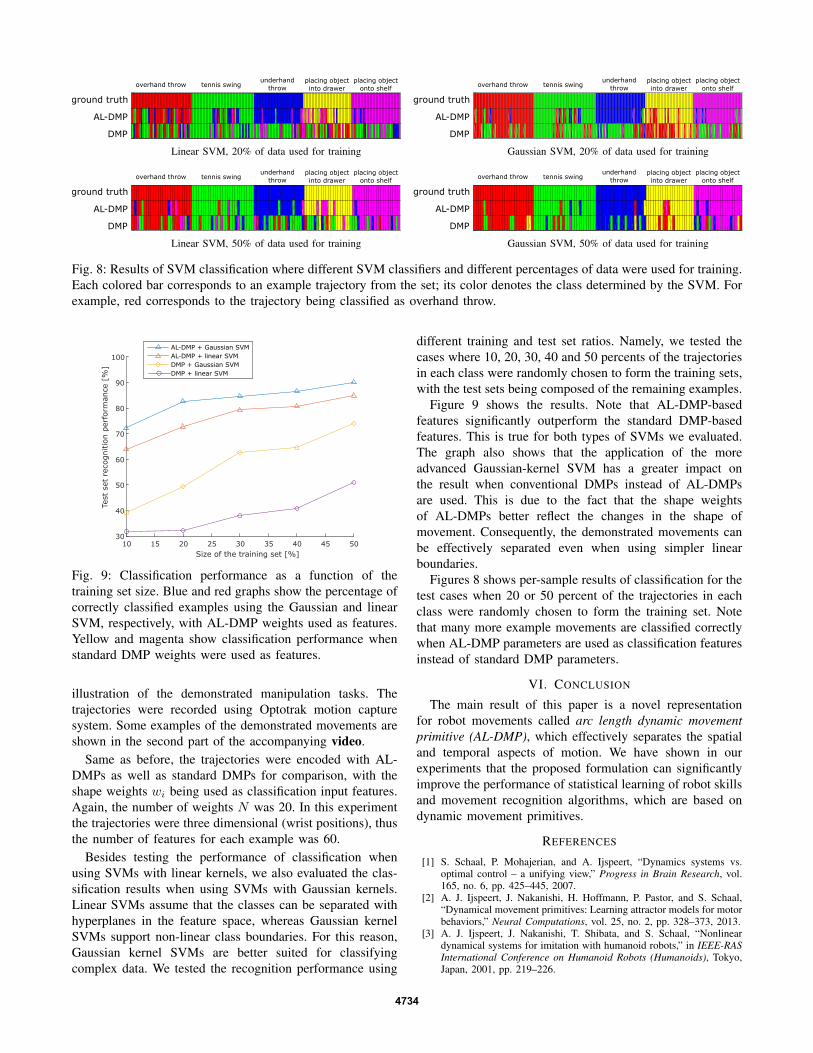
Fig. 8: Results of SVM classification where different SVM classifiers and different percentages of data were used for training.Each colored bar corresponds to an example trajectory from the set; its color denotes the class determined by the SVM. Forexample, red corresponds to the trajectory being classified as overhand throw.

Size of the training set [%]10 15 20 25 30 35 40 45 50

Test

set

rec

ognitio

n p

erfo

rman

ce [

%]

30

40

50

60

70

80

90

100AL-DMP + Gaussian SVMAL-DMP + linear SVMDMP + Gaussian SVMDMP + linear SVM

Fig. 9: Classification performance as a function of thetraining set size. Blue and red graphs show the percentage ofcorrectly classified examples using the Gaussian and linearSVM, respectively, with AL-DMP weights used as features.Yellow and magenta show classification performance whenstandard DMP weights were used as features.

illustration of the demonstrated manipulation tasks. Thetrajectories were recorded using Optotrak motion capturesystem. Some examples of the demonstrated movements areshown in the second part of the accompanying video.

Same as before, the trajectories were encoded with AL-DMPs as well as standard DMPs for comparison, with theshape weights wi being used as classification input features.Again, the number of weights N was 20. In this experimentthe trajectories were three dimensional (wrist positions), thusthe number of features for each example was 60.

Besides testing the performance of classification whenusing SVMs with linear kernels, we also evaluated the clas-sification results when using SVMs with Gaussian kernels.Linear SVMs assume that the classes can be separated withhyperplanes in the feature space, whereas Gaussian kernelSVMs support non-linear class boundaries. For this reason,Gaussian kernel SVMs are better suited for classifyingcomplex data. We tested the recognition performance using

different training and test set ratios. Namely, we tested thecases where 10, 20, 30, 40 and 50 percents of the trajectoriesin each class were randomly chosen to form the training sets,with the test sets being composed of the remaining examples.

Figure 9 shows the results. Note that AL-DMP-basedfeatures significantly outperform the standard DMP-basedfeatures. This is true for both types of SVMs we evaluated.The graph also shows that the application of the moreadvanced Gaussian-kernel SVM has a greater impact onthe result when conventional DMPs instead of AL-DMPsare used. This is due to the fact that the shape weightsof AL-DMPs better reflect the changes in the shape ofmovement. Consequently, the demonstrated movements canbe effectively separated even when using simpler linearboundaries.

Figures 8 shows per-sample results of classification for thetest cases when 20 or 50 percent of the trajectories in eachclass were randomly chosen to form the training set. Notethat many more example movements are classified correctlywhen AL-DMP parameters are used as classification featuresinstead of standard DMP parameters.

VI. CONCLUSION

The main result of this paper is a novel representationfor robot movements called arc length dynamic movementprimitive (AL-DMP), which effectively separates the spatialand temporal aspects of motion. We have shown in ourexperiments that the proposed formulation can significantlyimprove the performance of statistical learning of robot skillsand movement recognition algorithms, which are based ondynamic movement primitives.

REFERENCES

[1] S. Schaal, P. Mohajerian, and A. Ijspeert, “Dynamics systems vs.optimal control – a unifying view,” Progress in Brain Research, vol.165, no. 6, pp. 425–445, 2007.

[2] A. J. Ijspeert, J. Nakanishi, H. Hoffmann, P. Pastor, and S. Schaal,“Dynamical movement primitives: Learning attractor models for motorbehaviors,” Neural Computations, vol. 25, no. 2, pp. 328–373, 2013.

[3] A. J. Ijspeert, J. Nakanishi, T. Shibata, and S. Schaal, “Nonlineardynamical systems for imitation with humanoid robots,” in IEEE-RASInternational Conference on Humanoid Robots (Humanoids), Tokyo,Japan, 2001, pp. 219–226.

4734

[4] J. Kober and J. Peters, “Policy search for motor primitives in robotics,”Machine Learning, vol. 84, no. 1-2, pp. 171–203, 2010.

[5] A. Colome and C. Torras, “Dimensionality reduction and motioncoordination in learning trajectories with dynamic movement prim-itives,” in IEEE/RSJ International Conference on Intelligent Robotsand Systems (IROS), Chicago, IL, 2014, pp. 1414–1420.

[6] A. Ude, A. Gams, T. Asfour, and J. Morimoto, “Task-specific general-ization of discrete and periodic dynamic movement primitives,” IEEETransactions on Robotics, vol. 26, no. 5, pp. 800–815, 2010.

[7] T. Matsubara, S.-H. Hyon, and J. Morimoto, “Learning parametricdynamic movement primitives from multiple demonstrations,” NeuralNetworks, vol. 24, no. 5, pp. 493–500, 2011.

[8] E. Ruckert and A. d’Avella, “Learned parametrized dynamic move-ment primitives with shared synergies for controlling robotic andmusculoskeletal systems,” Frontiers in Computational Neuroscience,vol. 7, 2013.

[9] A. D. Dragan, K. Muelling, J. A. Bagnell, and S. S. Srinivasa, “Move-ment primitives via optimization,” in IEEE International Conferenceon Robotics and Automation (ICRA), Seattle, WA, 2015, pp. 2339–2346.

[10] P. Pastor, L. Righetti, M. Kalakrishnan, and S. Schaal, “Online move-ment adaptation based on previous sensor experiences,” in IEEE/RSJInternational Conference on Intelligent Robots and Systems (IROS),San Francisco, CA, 2011, pp. 365–371.

[11] F. J. Abu-Dakka, B. Nemec, J. A. Jørgensen, T. R. Savarimuthu,N. Kruger, and A. Ude, “Adaptation of manipulation skills in physicalcontact with the environment to reference force profiles,” AutonomousRobots, vol. 39, no. 2, pp. 199–217, 2015.

[12] A. Gams, B. Nemec, A. J. Ijspeert, and A. Ude, “Coupling movement

primitives: Interaction with the environment and bimanual tasks,”IEEE Transactions on Robotics, vol. 30, no. 4, pp. 816–830, 2014.

[13] T. Kulvicius, M. Biehl, M. J. Aein, M. Tamosiunaite, and F. Worgotter,“Interaction learning for dynamic movement primitives used in co-operative robotic tasks,” Robotics and Autonomous Systems, vol. 61,no. 12, pp. 1450–1459, 2013.

[14] B. Nemec, A. Gams, and A. Ude, “Velocity adaptation for self-improvement of skills learned from user demonstrations,” in IEEE-RASInternational Conference on Humanoid Robots (Humanoids), Atlanta,GA, 2013, pp. 423–428.

[15] R. Vuga, B. Nemec, and A. Ude, “Speed adaptation for self-improvement of skills learned from user demonstrations,” Robotica,pp. 1–17, 2015, doi: 10.1017/S0263574715000405.

[16] P. Englert, A. Paraschos, J. Peters, and M. P. Deisenroth, “Probabilisticmodel-based imitation learning,” Adaptive Behavior, vol. 21, no. 5, pp.388–403, 2013.

[17] H. Ben Amor, G. Neumann, S. Kamthe, O. Kroemer, and J. Peters,“Interaction primitives for human-robot cooperation tasks,” in IEEEInternational Conference on Robotics and Automation (ICRA), HongKong, China, 2014, pp. 2831–2837.

[18] H. Sakoe and S. Chiba, “Dynamic programming algorithm optimiza-tion for spoken word recognition,” IEEE Transactions on Acoustics,Speech and Signal Processing, vol. 26, no. 1, pp. 43–49, 1978.

[19] M. Ewerton, G. Maeda, J. Peters, and G. Neumann, “Learning motorskills from partially observed movements executed at different speeds,”in IEEE/RSJ International Conference on Intelligent Robots andSystems (IROS), Hamburg, Germany, 2015.

[20] C. Cortes and V. Vapnik, “Support-vector networks,” Machine Learn-ing, vol. 20, no. 3, pp. 273–297, 1995.

4735